Consumer Learning and Habit Formation with

Multiple Brand Choices

Valentin Agafonov∗

Advisor: Professor Ilya Segal

2007

This paper proposes a tractable structural model for the behavior of a

consumer who learns and forms habits from consumption. The consumer’s

dynamic programming problem is solved and applied to two sets of scanner

data on purchases of yogurt to estimate the model’s structural parameters

by maximum likelihood. Using ideas from multinomial logit, the consumer

is viewed as making purchase decisions faced with multiple brand choices.

Estimation of the model produces statistically significant estimates (as well

as dollar values) of both learning and habit formation in the data.

*I would like to thank Professor Segal for his encouraging and intellectually rigorous mentorship. Professor Segal’s insightful suggestions helped me better grasp the intuition behind economics. And his unwavering commitment to encouraging research has made my experience of writing a thesis very intellectually rewarding. I would like to thank Professor Geoffrey Rothwell for his many valuable suggestions and ideas for the project. I would like to thank Professor James Lattin for graciously providing Data Set 1 and I would like to thank Andrea Pozzi for graciously providing Data Set 2.

Contents

1 Introduction 4

1.1 Summary of Results . . . . . . . . . . . . . . . . . . . . . . . 7

2 Model 8

2.1 Solution to the Consumer’s Dynamic Programming Problem . 11

2.2 Special Cases of the Model . . . . . . . . . . . . . . . . . . . . 12

2.2.1 Consumer Learning . . . . . . . . . . . . . . . . . . . . 12

2.2.2 Habit Formation . . . . . . . . . . . . . . . . . . . . . 12

2.3 The Econometric Model (Multiple Brand Choices) . . . . . . . 12

2.3.1 Likelihood Function . . . . . . . . . . . . . . . . . . . . 18

2.4 Alternative Specifications . . . . . . . . . . . . . . . . . . . . . 19

3 Data 20

4 Estimation 23

4.1 Evidence from Data Set 1 . . . . . . . . . . . . . . . . . . . . 23

4.2 Evidence from Data Set 2 . . . . . . . . . . . . . . . . . . . . 32

5 Conclusion 37

A Solution to the Consumer’s Dynamic Programming Problem 40

A.1 The First Period Choice . . . . . . . . . . . . . . . . . . . . . 40

A.2 The Second Period Choice . . . . . . . . . . . . . . . . . . . . 42

2

B Likelihood of Consumer’s Decisions 43

B.1 Likelihood of Consumer’s First Period Decision . . . . . . . . 43

B.2 Conditional Likelihood of Consumer’s Second Period Decision 45

References 48

List of Tables

1 Data Sets Used . . . . . . . . . . . . . . . . . . . . . . . . . . 21

2 Estimated Model Parameters for Data Set 1 . . . . . . . . . . 24

3 Dynamic Effects Predictions versus Observed (Data Set 1) . . 25

4 Estimated Model Parameters for Data Set 2 . . . . . . . . . . 33

5 Dynamic Effects Predictions versus Observed (Data Set 2) . . 34

List of Figures

1 Learning Only Distribution of Reservation Price P2 . . . . . . 13

2 Habit Formation Only Distribution of Reservation Price P2 . . 14

3 Shifts in Demand (Data Set 1) . . . . . . . . . . . . . . . . . . 30

4 Demand (Data Set 1) . . . . . . . . . . . . . . . . . . . . . . . 31

5 Demand (Data Set 2) . . . . . . . . . . . . . . . . . . . . . . . 36

6 Reservation Price (Data Set 2) . . . . . . . . . . . . . . . . . . 37

3

1 Introduction

The dependence of consumer demand upon previous consumption, if it were

present to a significant degree in consumer decision making, would need to

be accounted for in models of consumer demand. Two important potential

sources of this path dependence in consumer demand are habit formation

and learning effects. There is a significant amount of literature on rational

habit formation — i.e. Becker and Murphy (1988). With habit formation,

a consumer’s demand for a product will be higher because the product was

consumed before. The other source of path dependence is learning. With ex-

perience goods, a consumer will not know with certainty her marginal benefit

of consuming the product prior to consuming it, and will have incentives to

experiment — i.e. trade off current utility for potential future utility by ac-

quiring information about a product now through consuming it now (i.e. see

Bergemann and Valimaki 1996). Therefore with learning consumer behavior

will depend on prior purchases of the product — those who have tried the

product before are more certain (and have more accurate predictions) about

their marginal benefit from consuming it than those who have not tried it

before. An important question is whether these habit formation and learning

effects are present to a significant degree in consumer behavior, because if

they were, they would have to be accounted for in demand derivations in or-

der to avoid biased estimates, and they could make current demand models

richer and lend them more explanatory power.

4

There are not many papers in the economics literature concerned with

measuring the sizes of these effects. One paper measures both habit forma-

tion and learning effects from scanner data (Osborne 2006). Other papers

(Ackerberg 2003;Erdem and Keane 1996; Crawford and Shum 2005) mea-

sure these effects as well, but none (except Osborne 2006) accounts for both

effects in the same demand model.

Using classical methods (MLE) for such a model can be computationally

demanding. Since modeling a consumer who is learning normally involves

an infinite horizon with uncertain future determinants of demand, a paper

attempting to model this behavior would solve the consumer’s problem by

backwards induction through time, and the larger the number of time pe-

riods, the larger the state space, the more computationally intensive calcu-

lations become — this is referred to as the “curse of dimensionality”. This

is further complicated by the fact that modeling learning involves persistent

(through time) unobserved variables which need to be integrated out in or-

der to calculate the likelihood of an observation. This integration does not

have a closed form and is simulated for each iteration of likelihood. To ease

the computational burden, approximations to the dynamic programming so-

lution are used by interpolating the solution from a subset of points in the

state space. Even with these simplifications, the estimation process is still

very computationally demanding. Additionally, using approximate solutions

to the consumer’s dynamic programming problem to estimate the structural

model by maximum likelihood has potential pitfalls, such as inconsistent

5

and biased parameter estimates (i.e. see Fernandez-Villaverde et al 2006,

finding that second-order errors in the approximate solution to the dynamic

programming problem can result in first-order errors in the approximated

likelihood). My goal in this paper is to derive a tractable model of consumer

learning and habit formation, and use this model to test the presence of these

effects in the behavior of consumers in two panel data sets of supermarket

shoppers (about 4000 consumers in one and about 11000 consumers in the

other data set)

Estimating both consumer learning and habit formation in the same

model has many advantages. For example, a model estimating habit for-

mation and not accounting for learning could be subject to the criticism that

estimates of habit formation reflect consumer learning (i.e. the consumer

tries the product, discovers her high valuation, and keeps buying it for that

reason and not because of habit formation). The advantage of the model in

this paper is that since learning is controlled for, such a bias should not be

present. Osborne points out that identifying learning without controlling for

habit formation is also subject to possible difficulties. He explains that habit

formation may make it look like there is less learning than there really is be-

cause it makes switching brands costly. But controlling for habit formation

should fix these difficulties as well.

Since Osborne (2005) is the only paper in the literature which estimates

learning and habit formation in the same model, it is the best paper to com-

pare with the estimates derived in this paper. It may be useful to observe

6

the differences between Osborne (2005) and this paper. Osborne applies his

model to scanner data on purchases of laundry detergent while this paper

applies its model to scanner data on purchases of yogurt. Since Osborne

uses a very rich heterogeneity structure in his model, he estimates it using

Markov Chain Monte Carlo, and this paper uses classical methods of estima-

tion (Maximum Likelihood).

1.1 Summary of Results

The paper develops a structural model of consumer demand using an exact

solution to the consumer’s dynamic programming problem and estimates it

using MLE. In Data Set 1, the parameter corresponding to the consumer’s

uncertainty about her true taste for yogurt has an estimate which is is highly

statistically significantly different from zero, with a value of 5.44 and a stan-

dard error of 0.664 (in Data Set 2 it has value 6.06 and standard error 0.142).

Using a Taylor series approximation, this translates into an estimate of 230

cents for the standard deviation of tastes, with the estimator’s standard error

at 153 cents (and in Data Set 2 standard deviation of tastes is 427 cents and

has a standard error of 60 cents). Thus consumers are very heterogeneous

in their tastes for yogurt, with some consumers liking it a lot, but others

not liking it. This indicates incentives for consumer learning. In Data Set 2

the habit formation estimate is highly statistically significantly different from

zero, with a value of 82 cents and a standard error of 8.14 cents. This esti-

mate indicates that consuming yogurt in period 1 increases the consumer’s

7

taste for it in the next period by 82 cents. Since most brands of yogurt in

the data sets cost between 50 cents and $1, the habit formation effect is very

significant.

2 Model

The model developped in this section is a structural model of consumer choice

which explicitly solves the consumer’s maximization problem as opposed to

a reduced form model. The advantages of a structural model include the

fact that, if the model is correctly specified, parameters of the model can be

taken away from the data (and, for example, used for counterfactuals/policy

experiments mindful of the Lucas critique). Another advantage of the struc-

tural model is that when estimated by Maximum Likelihood it captures more

information from the data than a reduced form model would. This advan-

tage is especially relevant for this paper because a reduced form specification

failed to detect statistically significant learning and habit formation in the

data because it discarded too much relevant information. The reduced form

model is discussed in section 2.4.

Consumer behavior which is subject to learning can result from the con-

sumer not being certain about her marginal benefit of consuming the product

until she consumes it — this could be true of pure experience goods, but may

be true of all products to some degree. Thus there is a component to utility

which is unknown before the first consumption event, but is revealed after

8

it. A consumer’s first purchase event is a gamble because marginal utility

of consumption is unknown at that time, but once a first purchase is made,

the consumer acquires information about her marginal utility of consuming

the product, and hence, for potential future purchase events, has accurate

information about her valuation. Thus in a first purchase the consumer not

only derives utility from immediate consumption, but also acquires valuable

information for consumption in future periods. While the consumer does

not derive utility from this information directly, she uses it to make choices

maximizing total expected utility. Therefore the consumer may want to

trade off utility from immediate consumption for information. These trade-

offs are built into the behavior of a forward-looking consumer who maximizes

ecpected total utility rather than immediate utility.

We assume consumers have von Neumann-Morgenstern form utility, hence

they maximize expected total utility in the face of uncertain future outcomes

rather than just deterministic total utility (which would be impossible here

in the presence of random variables affecting utility). This is a two-period

model, so we assume customers do not appreciably discount the future. One

advantage of a two-period model is the existence of a closed-form solution to

the dynamic programming problem. Another advantage is the tractability of

the two-period model.

Define the total utility of a two-period consumption choice as

U = vx1,x2 + x1(ε1 − P1 + η) + x2(ε2 − P2 + η), (1)

9

And

v1,1 − v1,0 > v0,1 − v0,0 (2)

so define

δ = (v1,1 − v1,0) − (v0,1 − v0,0) . (3)

where the purchase decisions xk ∈ {0, 1} so the consumer chooses to consume

one unit of the product or zero units, depending on which of these options

yields the higher expected utility. The εk are standard Random Utility Model

distrubances, and here they account for effects of unobservable factors on

the utility. Pk are prices for the product. The η is the unknown component

of utility which will be used to capture learning effects — it is observed

by the agent through consuming the product only if and after she makes

a purchase in the first period, and does not change with time, hence the

information acquired by a first period purchase event is very valuable. The

agent observes ε1 and P1 before deciding on x1, and observes ε2 and P2

before deciding on x2. The δ is used to capture habit formation — a positive

value on δ indicates that the marginal utility of consuming a product will

be higher in period 2 if the product was consumed in period 1. εk, η, and

P2 are assumed normally distributed. Normalize E(η) = 0, while E(ε) can

be nonzero. Therefore, when a consumer purchases yogurt, she buys three

things: immediate consumption, an increase in next period’s utility (through

habit formation), and information.

For the benefit of the model with multiple brands in Section 2.3, introduce

10

the intercept r into both periods’ flow utility. Assume this intercept is known

to the consumer before the first period. This amounts to adding r(x1 + x2)

to the utility specified in equation 1.

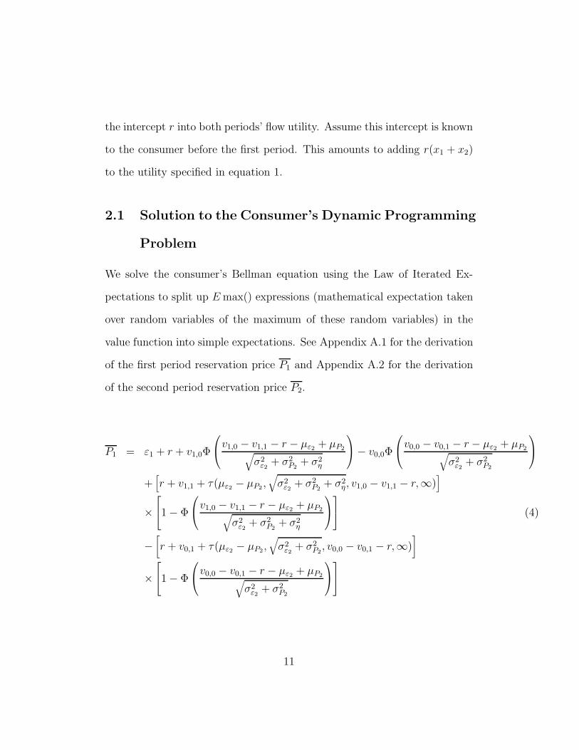
2.1 Solution to the Consumer’s Dynamic Programming

Problem

We solve the consumer’s Bellman equation using the Law of Iterated Ex-

pectations to split up E max() expressions (mathematical expectation taken

over random variables of the maximum of these random variables) in the

value function into simple expectations. See Appendix A.1 for the derivation

of the first period reservation price P1 and Appendix A.2 for the derivation

of the second period reservation price P2.

P1 = ε1 + r + v1,0Φ

⎛⎝v1,0 − v1,1 − r − με2 + μP2√

σ2ε2

+ σ2P2

+ σ2η

⎞⎠ − v0,0Φ

⎛⎝v0,0 − v0,1 − r − με2 + μP2√

σ2ε2

+ σ2P2

⎞⎠

+[r + v1,1 + τ(με2 − μP2 ,

√σ2

ε2+ σ2

P2+ σ2

η , v1,0 − v1,1 − r,∞)]

×⎡⎣1 − Φ

⎛⎝v1,0 − v1,1 − r − με2 + μP2√

σ2ε2

+ σ2P2

+ σ2η

⎞⎠

⎤⎦ (4)

−[r + v0,1 + τ(με2 − μP2,

√σ2

ε2+ σ2

P2, v0,0 − v0,1 − r,∞)

]

×⎡⎣1 − Φ

⎛⎝v0,0 − v0,1 − r − με2 + μP2√

σ2ε2

+ σ2P2

⎞⎠

⎤⎦

11

[P2

∣∣∣ x1

]= r + (v0,1 − v0,0) + ε2 + x1(δ + η) (5)

2.2 Special Cases of the Model

In order to see the effect of this x1(δ + η) term on demand dynamics, we

observe the components of this effect in two special cases of the model.

2.2.1 Consumer Learning

• Set δ = v0,0 = v0,1 = v1,0 = v1,0 ≡ 0. This will be a pure learning model.

Then P2 |x1=1 = P2 |x1=0 + η. And η is stochastic with E(η) = 0. Thus

P2 |x1=1 is a mean preserving spread of P2 |x1=0 . Hence P2 |x1=0 Second

Order Stochastically Dominates P2 |x1=1 . See Figure 1.

2.2.2 Habit Formation

• Set η = ση ≡ 0. This will be a pure habit formation model. Then

P2 |x1=1 = P2 |x1=0 + δ. Thus P2 |x1=1 First Order Stochastically Dom-

inates P2 |x1=0 . see Figure 2.

2.3 The Econometric Model (Multiple Brand Choices)

In this section the econometric model which will be used to apply the eco-

nomic model to the data is discussed. The economic model solution derived

above represents optimal behavior for a consumer, which is the subject of

12

Figure 1: Learning Only Distribution of Reservation Price P2

CumulativeProbability

P2

F( |x = 1)P2 1

F( |x = 0)P2 1

interest in this paper. The goal in this section is to get the most out of

the data available in order to gain knowledge about the underlying behavior

described by the economic model. Firstly, the model in this section will go

forward from single brand to multiple brand, which is done for the following

reasons:

1 Data Coverage The panel data sets which are available for this paper

include information about transactions for many brands/flavors of yo-

gurt. One way of getting the most out of this data is to treat each brand

of yogurt as a “type” of the same product and thereby incorporate a

13

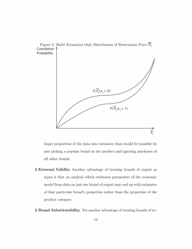
Figure 2: Habit Formation Only Distribution of Reservation Price P2

CumulativeProbability

P2

F( |x = 1)P2 1

F( |x = 0)P2 1

larger proportion of the data into estimates than would be possible by

just picking a popular brand as the product and ignoring purchases of

all other brands.

2 External Validity Another advantage of treating brands of yogurt as

types is that an analysis which estimates parameters of the economic

model from data on just one brand of yogurt may end up with estimates

of that particular brand’s properties rather than the properties of the

product category.

3 Brand Substitutability Yet another advantage of treating brands of yo-

14

gurt as types is that, if the brands are sufficiently substitutable, changes

in the price (or other characteristic) of one brand may have an effect

on demand for other brands.

Consumers often do not make choices about purchases in isolation from

alternatives: choices available to the consumer matter. For example, when

choosing a yogurt, consumers have a variety of brands and flavors available

to them, and even if maximizing the flow utility of every one of these choices

separately would yield decisions to buy one unit rather than buy zero units,

consumers do not buy every yogurt in the store. In fact, assuming the con-

sumer has unit demand for yogurt, and also has an available outside good

(not buying any yogurt), then it would make sense for the consumer to select

the yogurt which yields the highest surplus (i.e. the yogurt the purchase

of which will yield highest expected utility over the consumer’s horizon).

Alternatively, purchases of different brands of yogurt could be modeled as

independent of one another, but it seems probable that brands are substi-

tutable, thus I model choice between brands.

In order to econometrically express the idea that the consumer selects the

best from a number of alternatives we apply some ideas behind McFadden’s

model of multinomial choice (multinomial logit), specifically, the assumption

of Independence of Irrelevant Alternatives. Only part of the derivation from

McFadden (1975) is used because this paper makes different assumptions

about the error term ε than those of standard multinomial logit.

15

The utility in the economic model, when allowed to apply to different

brands and individuals, takes the following form for brand/flavor j and in-

dividual i:

U ji = rj(xji1 + xji

2 ) + vxji1 ,xji

2+ xji

1 (εji1 − P j

1 + ηji) + xji2 (εji

2 − P j2 + ηji) (6)

The statistician does not observe the εjik and ηji and considers them stochas-

tic, while με, σε, ση, μP2, σP2 (which represent beliefs of the consumers, and

in the case of P2, not necessarily the actual mean and standard deviation

of observed prices) and v1,1, v0,1, v0,0, δ, rj are deterministic parameters of the

model.1 We assume v1,1, v0,1, v0,0, δ, με, σε, ση, μP2, σP2 are specific to the prod-

uct, and hence are the same for every brand/flavor. We also assume these

parameters are the same for every individual in the data — the only vari-

ables varying by individual are εjik and ηji. The intercept rj accounts for

the possibility of differences (vertical differentiation) between brands/flavors

— i.e. differences which all consumers would agree on, hence they are not

accounted for by the “error” term ε.

The statistician does not observe all the variables which enter into the

customer’s utility and affect the customer’s decisions, thus the statistician

assigns probabilities to decisions to buy or not buy a brand/flavor based on

the information set consisting of observed variables and distribution assump-

tions about the stochastic unobserved variables. Denote the probability of

1Assume σε1 = σε2 ≡ σε and με1 = με2 ≡ με

16

selecting alternative n from a nonempty set of choices N by pN(n). Assume

pN(n) > 0 for all n ∈ N . Then assume Independence from Irrelevant

Alternatives (IIA): if n, m ∈ N , then

p{n,m}(n)

p{n,m}(m)=

pN(n)

pN (m)(7)

This is a strong assumption, but it is a standard one because it makes it

possible to evaluate likelihood without calculating the cdf for multivariate

distributions, a task which is extremely computationally intensive.

Define an arbitrary index for the brands/flavors available to the consumer,

and for convenience set the index of the “none” choice (none of the available

brand/flavors purchased) to 0.

The likelihood of the consumer’s first period choice l1 is derived in Ap-

pendix B.1 and the likelihood of the consumer’s second period choice l2 is

derived in Appendix B.2.

For l1 �= 0

pN(l1) =1 − Φ

(P s

1−cl1−με

σε

)

Φ(

P s1−cl1−με

σε

)/⎛

⎝1 +∑

m∈N,m�=0

1 − Φ(

P s1−cm−με

σε

)Φ

(P s

1−cm−με

σε

)⎞⎠ (8)

and for l1 = 0

pN(l1) = 1

/⎛⎝1 +

∑m∈N,m�=0

1 − Φ(

P s1−cm−με

σε

)Φ

(P s

1−cm−με

σε

)⎞⎠ (9)

17

For l2 �= 0

pN( l2| l1) =

[1 − Φ

(P

l22 −c

l22 −δ−με√

σ2ε+σ2

η

)]1(l1=l2) [1 − Φ

(P

l22 −c

l22 −με

σε

)]1−1(l1=l2)

[Φ

(P

l22 −c

l22 −δ−με√

σ2ε+σ2

η

)]1(l1=l2) [Φ

(P

l22 −c

l22 −με

σε

)]1−1(l1=l2)(10)

÷

⎛⎜⎜⎜⎝1 +

∑m∈N,m�=0

[1 − Φ

(P m

2 −cm2 −δ−με√

σ2ε+σ2

η

)]1(l1=m) [1 − Φ

(P m

2 −cm2 −με

σε

)]1−1(l1=m)

[Φ

(P m

2 −cm2 −δ−με√

σ2ε+σ2

η

)]1(l1=m) [Φ

(P m

2 −cm2 −με

σε

)]1−1(l1=m)

⎞⎟⎟⎟⎠

and for l2 = 0

pN( l2| l1) =

⎛⎜⎜⎜⎝1 +

∑m∈N,m�=0

[1 − Φ

(P m

2 −cm2 −δ−με√

σ2ε+σ2

η

)]1(l1=m) [1 − Φ

(P m

2 −cm2 −με

σε

)]1−1(l1=m)

[Φ

(P m

2 −cm2 −δ−με√

σ2ε+σ2

η

)]1(l1=m) [Φ

(P m

2 −cm2 −με

σε

)]1−1(l1=m)

⎞⎟⎟⎟⎠

−1

(11)

2.3.1 Likelihood Function

The likelihood of an observation with choice b1 for the first stage and choice b2

for the second stage is Pr(l1 = b1, l2 = b2) = Pr(l2 = b2|l1 = b1)×Pr(l1 = b1).

Thus likelihood is

L = pN(b2| b1)pN(b1) (12)

and L is computed by plugging in pN(b2| b1) and pN(b1) from equations

(8),(9),(10),(11).

18

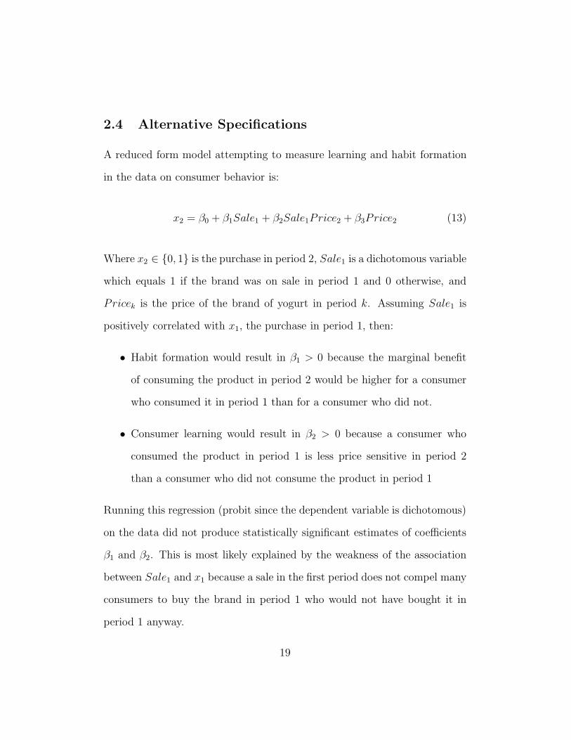
2.4 Alternative Specifications

A reduced form model attempting to measure learning and habit formation

in the data on consumer behavior is:

x2 = β0 + β1Sale1 + β2Sale1Price2 + β3Price2 (13)

Where x2 ∈ {0, 1} is the purchase in period 2, Sale1 is a dichotomous variable

which equals 1 if the brand was on sale in period 1 and 0 otherwise, and

Pricek is the price of the brand of yogurt in period k. Assuming Sale1 is

positively correlated with x1, the purchase in period 1, then:

• Habit formation would result in β1 > 0 because the marginal benefit

of consuming the product in period 2 would be higher for a consumer

who consumed it in period 1 than for a consumer who did not.

• Consumer learning would result in β2 > 0 because a consumer who

consumed the product in period 1 is less price sensitive in period 2

than a consumer who did not consume the product in period 1

Running this regression (probit since the dependent variable is dichotomous)

on the data did not produce statistically significant estimates of coefficients

β1 and β2. This is most likely explained by the weakness of the association

between Sale1 and x1 because a sale in the first period does not compel many

consumers to buy the brand in period 1 who would not have bought it in

period 1 anyway.

19

3 Data

In order to test the presence of learning and habit formation in consumer

behavior, and to measure the sizes of these effects, we turn to revealed pref-

erence data for supermarket shoppers.

Using this type of data (revealed preference) has the advantage that the

economic agents in the data have the correct incentives (they are shopping

normally) and they are experienced and knowledgeable about optimizing

their decisions in this setting. The data sets used are scanner data for pur-

chases of yogurt. Two data sets were used, one with transactions of approxi-

mately 4000 consumers followed over a period of two years, and another with

approximately 11000 consumers also followed over a period of approximately

two years.

20

Table 1: Data Sets Used

Data Set Final Number of Consumers in Data

Data Set 1 3384Data Set 2 8650

21

In each of the data sets, for each customer i, a random week ti is picked

as a starting point. A random week is picked for each consumer in order

to insure prices vary in the data used (for identification purposes) since the

prices may be very similar for all consumers in the same week. Another

reason to pick a random week for each consumer is that it helps to sidestep

potential difficulties associated with measuring the purchasing behavior of

different consumers in the same week because the unobserved variables af-

fecting utility may be correlated across consumers on the same date. The

customer’s purchase or lack thereof of 35 brands of yogurt at ti is recorded.

Since the learning and habit formation effects we are attempting to isolate

are intertemporal consumption effects, we attempt to remove other, poten-

tially confounding, intertemporal effects from the data proactively so that

any statistical association we find can confidently be attributed to our spe-

cific intertemporal consumption effects of interest and not other potentially

confounding effects. One such effect is storage — a consumer may purchase a

product at one time, form a rational habit for it, but not purchase it again at

the next opportunity only because she has stored a sufficient amount of the

product from her first period purchase. This hypothetical behavior would

create a downward bias on habit formation estimates. Thus, in order to

minimize storage effects, we look at the consumer’s shopping trip four weeks

after the original trip date ti, and refer to this date as t′i = ti + 4. The

customer’s purchase or lack thereof of 35 brands of yogurt at t′i is recorded.

Because we are attempting to measure learning effects, we also drop any

22

consumer i who purchased any of the 35 brands of yogurt four weeks or less

prior to ti from our data. Even if brand j of yogurt was not purchased by

consumer i during week t′i or week ti, we still record the price that we expect

consumer i observed of yogurt brand j in that week. This is done by check-

ing the price observed in a purchase of the same brand of yogurt j in the

same week in the same store (by another consumer). Since the multibrand

model, as is common in the literature, assumes the consumer purchases no

more than one brand of yogurt on each shopping trip, observations where

consumer i purchases more than one brand of yogurt during week t′i or week

ti are dropped.

4 Estimation

The maximum likelihood estimation results are shown in Table 2 for Data

Set 1 and in Table 4 for Data Set 2. v0,0 was normalized to zero, and so was

r0, the brand-specific intercept for brand 0 (not buying anything). Thus the

utility of purchasing nothing is zero. Prices in the data are given in cents.

4.1 Evidence from Data Set 1

23

Table 2: Estimated Model Parameters for Data Set 1

Parameter Estimate Parameter Estimate Parameter Estimate

ln(σε) 5.119139 ln(r8) 5.296639 ln(r23) 5.018946(0.2026432) (0.4201343) (0.5572788)

με -668.8425 ln(r9) 5.121379 ln(r24) 5.02987(154.6298) (0.5021016) (0.5489833)

ln(σP2 ) 4.904234 ln(r10) 5.13403 ln(r25) 5.153828(6.171514) (0.4912067) (0.5025538)

μP2 -1.091621 ln(r11) -4.997847 ln(r26) -3.128203(782.3295) (31.97883) (182.4084)

ln(ση) 5.438941 ln(r12) 4.999525 ln(r27) 5.181113(0.6640285) (0.5903094) (0.4771504)

δ 80.35355 ln(r13) -4.963921 ln(r28) 5.179468(165.7878) (34.20364) (0.4754916)

ln(v1,1) 4.152634 ln(r14) 5.203751 ln(r29) -2.726739(2.427955) (0.4679177) (161.2342)

ln(v0,1) -11.33953 ln(r15) 5.198169 ln(r30) 4.954935(2229.194) (0.4659872) (0.6175905)

ln(r1) 5.379895 ln(r16) 5.022056 ln(r31) 5.167926(0.3962141) (0.5546964) (0.4799807)

ln(r2) 5.484487 ln(r17) 5.340205 ln(r32) 4.842411(0.3577982) (0.4052718) (0.6913984)

ln(r3) 5.416172 ln(r18) 4.998615 ln(r33) -2.630624(0.3753905) (0.5919309) (141.8869)

ln(r4) 5.002529 ln(r19) 5.270693 ln(r34) -4.137877(0.5894222) (0.4346098) (239.6542)

ln(r5) 5.403721 ln(r20) 5.00915 ln(r35) -4.062496(0.3828157) (0.5671102) (232.3306)

ln(r6) 5.482439 ln(r21) 4.974899(0.3592197) (0.6360194)

ln(r7) 5.42788 ln(r22) 5.029355(0.376878) (0.5785778)

Note: Standard errors are in parentheses.

24

Table 3: Dynamic Effects Predictions versus Observed (Data Set 1)

Purchase Probabilities Predicted Observed

Pr (x2 = 0|x1 = 1) 0.9453 1Pr (x2 = 1|x1 = 1) 0.0547 0Pr (x2 = 0|x1 = 0) 0.9993 0.9983Pr (x2 = 1|x1 = 0) 0.0007 0.0017

Note: Calculation of predicted values relies on the observed sample standarddeviation and mean of P2. Observed probabilities are empirical frequenciesin the data.

25

The με estimate helps pin down the population average of consumer tastes

for yogurt, με + rj , where rj is the intercept for brand j — for example, for

brand 1, the population average is -452 cents. We will continue to use brand

1 whenever discussion requires a specific brand example. To be more spe-

cific, -452 cents is the population average of consumer tastes for nonbuyers

(x1 = x2 = 0), which are the majority. The population average for con-

sumers who buy in both periods is -388 cents, and for consumers who only

buy in the second period is -452 cents, and for consumers who only buy in

the first period is -469 cents. It may at first appear that people don’t like

yogurt very much and would prefer no yogurt to yogurt, but this is not ex-

actly what takes place. The parameter ln(ση) corresponds to the variation

in intrinsic taste for yogurt in the population, as well as the consumer’s un-

certainty about her true taste for yogurt. The estimate is highly statistically

significantly different from zero, with a value of 5.44 and a standard error of

0.664. Using a Taylor series approximation to estimate the standard error of

the coefficient’s transformation, this translates into an estimate of 230 cents

for ση with the estimator’s standard error at 153 cents. Thus consumers are

very heterogeneous in their tastes for yogurt, with some consumers liking

it a lot, but others not liking it. This result, the highly negative average

consumer taste tempered by a large degree of variation in consumer tastes,

can be seen in almost all brands in the data, and is also found in Osborne

(2005). Osborne points out that this wide heterogeneity in tastes points to

the “experience good” nature of the product. One of the estimates for the

26

consumer’s uncertainty about her true taste for the product in Osbourne can

be converted to cents to yield a standard deviation of 53 cents (this param-

eter is compared to this paper’s ση which represents both variation in true

tastes and consumer uncertainty about true tastes).

The δ estimate indicates that consuming brand j in period 1 increases the

consumer’s taste for the product in period 2 by 80 cents. This corresponds

to habit formation. The habit formation estimate which can be calculated

from the model estimated in Osborne is 44 cents (calculated by dividing the

habit formation coefficient by the MRS). Osborne finds that there is a lot of

individual heterogeneity in the degree of habit formation, and that 62% of

households are habit formers.

While habit formation can be easily interpreted by looking at the model

coefficients, consumer learning is not as straightforward to point out in the

numbers with an estimated model. Firstly, the highly statistically significant

coefficient on ln(ση), in other words, high degree of heterogeneity in consumer

tastes not revealed prior to the first consumption event, indicates strong in-

centives for consumers to learn: if consumer tastes have a large variance, and

consumers know this, they know that they receive valuable rewards from ex-

perimentation with brands. Osborne suggests that learning can be identified

in consumer behavior by looking at the difference between the share of con-

sumers who buy the product in the first period but do not repurchase it and

the share of consumers who do not buy the product in the first period but

buy it in the next period. The intuition here would be that those who pur-

27

chase but do not repurchase the product learned their true valuation of the

product by experimentation. But those who do not purchase right away but

purchase later represent the share of consumers who can be expected in the

second period to have seen high enough realizations of εi and perhaps low

enough realizations of price — thus this is a predictor of what proportion of

consumers can be expected to, in any period, purchase the product because

they are in the high tail of the distribution of unobservables for that period.

Hence large values of the difference between the two shares (in this paper,

probabilities) should be a good signal of learning in consumer behavior. We

can observe this identifier in Table 3. The difference in probabilities is almost

1, the maximum possible. Hence this is another indication of learning in the

data.

With estimates of the structural model it is also possible to examine coun-

terfactuals. Consider the consumer’s dynamic programming value function,

given the consumer purchases the brand in period 1, EV |x1=1. Then consider

a counterfactual in which the consumer does not learn from consumption but

does form habits — in other words, remove the learning from the consumer’s

optimization problem by specifying η = ση ≡ 0. Denote the consumer’s value

function in this counterfactual EV ′|x1=1. Calculating EV |x1=1 − EV ′|x1=1

should yield a measure of how much better off the consumer expects to be

because of the ability to learn about her product valuation through consump-

tion. Here the value is 17 cents, which may upon first examination seem low,

but really is not considering its frame of reference. Almost all of the brands

28

of yogurt in the sample cost between 50 cents and $1, hence 17 cents is a

significant change in valuation when compared to the cost of the product.

Comparing the estimate of habit formation, that the consumer’s taste for the

brand in the second period increases by 80 cents if the product is consumed

in the first period, to the prices of yogurt in the sample, indicates that the

effect of habit formation is just as large as the effect of price.

The estimated parameters of the structural model allow us to examine

demand for yogurt. Period 2 demand is:

Pr(P2 > P2

∣∣∣ P2

)= 1 − F (P2) (14)

where P2 has cdf F and the probability is over the εi2’s and ηi’s (consumers).

The effects of consumer learning and habit formation on demand can be

seen in Figure 3. The graph shows the differences implied by the model and

estimated parameters between demand given x1 = 0 and given x1 = 1. If the

product is purchased in the first period, habit formation shifts demand up by

80 cents and learning makes consumers less price sensitive hence the change in

slope. But the difference between demand given x1 = 0 and given x1 = 1 can

only be conveniently decomposed into its basic component effects in this view,

which includes negative values of price. When we look at the region of the

demand curve estimated in Figure 4 where only positive prices are considered,

the differences between the two curves are not obviously attributable to one

effect or the other. Thus the structural model provides intuition, which is

29

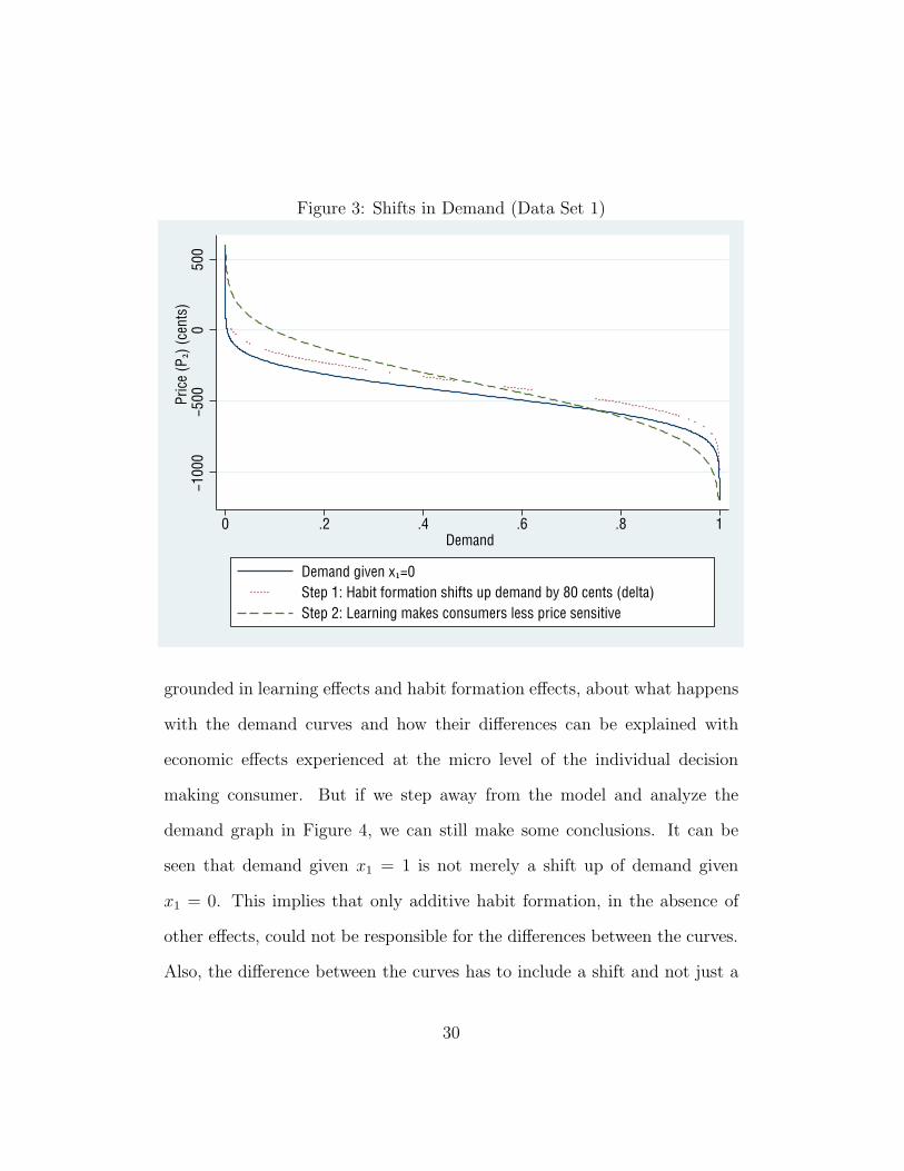
Figure 3: Shifts in Demand (Data Set 1)−1

000

−500

050

0Pr

ice

(P2)

(cen

ts)

0 .2 .4 .6 .8 1Demand

Demand given x1=0Step 1: Habit formation shifts up demand by 80 cents (delta)Step 2: Learning makes consumers less price sensitive

grounded in learning effects and habit formation effects, about what happens

with the demand curves and how their differences can be explained with

economic effects experienced at the micro level of the individual decision

making consumer. But if we step away from the model and analyze the

demand graph in Figure 4, we can still make some conclusions. It can be

seen that demand given x1 = 1 is not merely a shift up of demand given

x1 = 0. This implies that only additive habit formation, in the absence of

other effects, could not be responsible for the differences between the curves.

Also, the difference between the curves has to include a shift and not just a

30

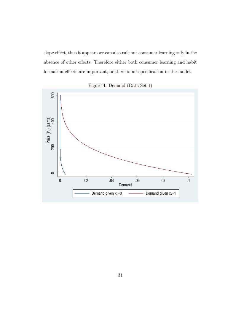
slope effect, thus it appears we can also rule out consumer learning only in the

absence of other effects. Therefore either both consumer learning and habit

formation effects are important, or there is misspecification in the model.

Figure 4: Demand (Data Set 1)

020

040

060

0Pr

ice

(P2)

(cen

ts)

0 .02 .04 .06 .08 .1Demand

Demand given x1=0 Demand given x1=1

31

4.2 Evidence from Data Set 2

The με estimate is necessary to calculate average consumer tastes. -700 cents

is the population average of consumer tastes for nonbuyers (x1 = x2 = 0),

which are the majority. The population average for consumers who buy in

both periods is -669 cents, and for consumers who only buy in the second

period is -700 cents, and for consumers who only buy in the first period

is -751 cents. As in Data Set 1, this does not mean people do not like

yogurt. The parameter ln(ση) corresponds to the variation in intrinsic taste

for yogurt in the population, as well as the consumer’s uncertainty about

her true taste for yogurt. The estimate is highly statistically significantly

different from zero, with a value of 6.06 and a standard error of 0.142. Using a

Taylor series approximation to estimate the standard error of the coefficient’s

transformation, this translates into an estimate of 427 cents for ση with the

estimator’s standard error at 60 cents. Thus, as in Data Set 1, consumers

are very heterogeneous in their tastes for yogurt, with some consumers liking

it a lot, but others not liking it. This is shown in Figure 6.

32

Table 4: Estimated Model Parameters for Data Set 2

Parameter Estimate Parameter Estimate Parameter Estimate

ln(σε) 5.53991 ln(r8) 3.947013 ln(r23) 3.693937(0.0164833) (0.5691153) (0.7270177)

με -827.8881 ln(r9) 2.919857 ln(r24) -5.10243(4.058027) (1.673276) (66.53002)

ln(σP2 ) 23.36663 ln(r10) 4.674613 ln(r25) 3.649968(.) (0.2023852) (0.8332664)

μP2 1.335668 ln(r11) 3.952077 ln(r26) -5.918308(.) (0.707396) (.)

ln(ση) 6.056033 ln(r12) 6.049533 ln(r27) 4.689607(0.1416533) (0.0494318) (0.2062894)

δ 82.31698 ln(r13) 2.190537 ln(r28) 4.051851(8.140572) (2.378045) (0.4674159)

ln(v1,1) 3.436761 ln(r14) 6.009966 ln(r29) 4.458556(0.1701274) (0.0555648) (0.2870664)

ln(v0,1) -8.309021 ln(r15) -5.162236 ln(r30) 3.989435(202.2424) (.) (0.5214765)

ln(r1) 4.84797 ln(r16) 3.616467 ln(r31) 4.268801(0.161968) (0.7956624) (0.3447859)

ln(r2) 2.906048 ln(r17) 4.155919 ln(r32) -12.76221(1.688454) (0.4252708) (1831.423)

ln(r3) 2.887012 ln(r18) 3.637418 ln(r33) 5.667088(1.649668) (0.6763644) (0.0703793)

ln(r4) 4.70944 ln(r19) 4.149523 ln(r34) 4.691722(0.2004381) (0.3967899) (0.1878336)

ln(r5) 4.773026 ln(r20) 4.429662 ln(r35) -5.227693(0.1789292) (0.2675972) (2.812465)

ln(r6) 4.765643 ln(r21) 4.171555(0.1854232) (0.3809042)

ln(r7) 4.638903 ln(r22) 4.070337(0.2216636) (0.4880038)

Note: the numbering of product brands in the two data sets is different,therefore brand number j in the first data set is not the same brand as brandnumber j in the second data set. Standard errors are in parentheses.

33

Table 5: Dynamic Effects Predictions versus Observed (Data Set 2)

Purchase Probabilities Predicted Observed

Pr (x2 = 0|x1 = 1) 0.9170 0.9259Pr (x2 = 1|x1 = 1) 0.0830 0.0741Pr (x2 = 0|x1 = 0) 0.9988 0.9950Pr (x2 = 1|x1 = 0) 0.0012 0.0050

Note: Calculation of predicted values relies on the observed sample standarddeviation and mean of P2. Observed probabilities are empirical frequenciesin the data.

34

The δ estimate is highly statistically significantly different from zero,

with a value of 82 and a standard error of 8.14. This estimate indicates that

consuming brand j in period 1 increases the consumer’s taste for the product

in period 2 by 82 cents. This corresponds to habit formation.

The large estimate for ση is an indication of significant incentives for con-

sumer learning. Another way to identify learning is to observe the difference

between the share of consumers who buy the product in the first period but

do not repurchase it and the share of consumers who do not buy the product

in the first period but buy it in the next period. Large values of the difference

between the two shares (in this paper, probabilities) should be a good signal

of learning in consumer behavior. We can observe this identifier in Table

5. The difference in probabilities is almost 1, the maximum possible. Hence

this is another indication of learning in the data.

A calculation of EV |x1=1 − EV ′|x1=1, which should yield a measure of how

much better off the consumer expects to be because of the ability to learn

about her product valuation through consumption, results in 30 cents. Recall

that almost all of the brands of yogurt in the sample cost between 50 cents

and $1, hence 30 cents is a significant change in valuation when compared

to the cost of the product. Comparing the estimate of habit formation, that

the consumer’s taste for the brand in the second period increases by 82 cents

if the product is consumed in the first period, to the prices of yogurt in the

sample, indicates that the effect of habit formation is just as large as the

effect of price.

35

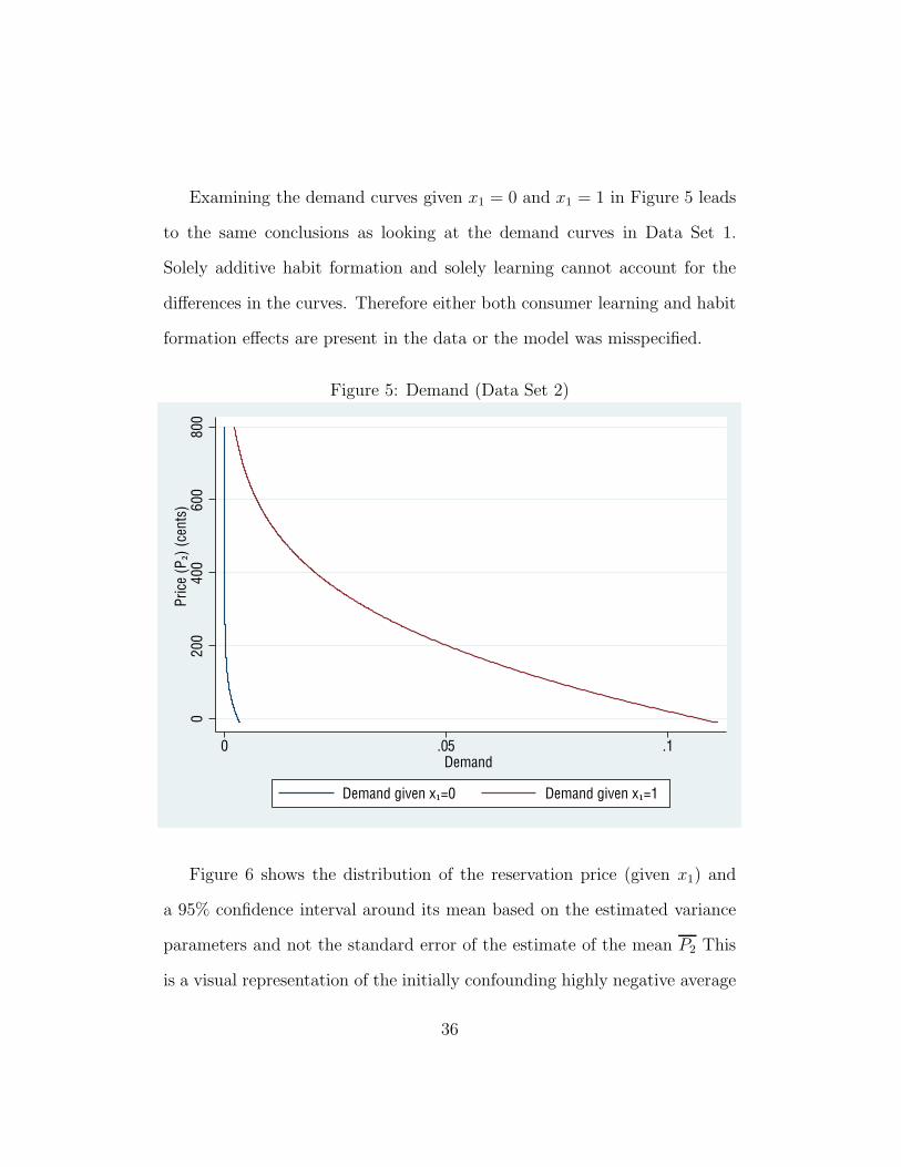
Examining the demand curves given x1 = 0 and x1 = 1 in Figure 5 leads

to the same conclusions as looking at the demand curves in Data Set 1.

Solely additive habit formation and solely learning cannot account for the

differences in the curves. Therefore either both consumer learning and habit

formation effects are present in the data or the model was misspecified.

Figure 5: Demand (Data Set 2)

020

040

060

080

0Pr

ice

(P2)

(cen

ts)

0 .05 .1Demand

Demand given x1=0 Demand given x1=1

Figure 6 shows the distribution of the reservation price (given x1) and

a 95% confidence interval around its mean based on the estimated variance

parameters and not the standard error of the estimate of the mean P2 This

is a visual representation of the initially confounding highly negative average

36

taste for every single brand of yogurt. The negative average is offset by

the very large variation around the mean in reservation price, hence the

heterogeneity in tastes for yogurt, and the fact that some people like a brand

of yogurt a lot while others do not like it at all.

Figure 6: Reservation Price (Data Set 2)

0.1

.2.3

.4De

nsity

−1595 −1199 −700 −618 −201 0 359 500Reservation Price (cents)

95% CI [P2|x1=1] 95% CI [P2|x1=0]Pr(P2|x1=1) Pr(P2|x1=0)

5 Conclusion

In this paper a tractable dynamic structural model for the intertemporal

purchasing behavior of a consumer which accounts for consumer learning

37

and habit formation was derived. The consumer’s dynamic programming

problem was solved exactly and the solution was used to estimate a model of

purchasing behavior with multiple brand choices using Maximum Likelihood.

The model was estimated on two sets of scanner data of purchases of yogurt.

The predictions from the two data sets were similar and yielded statistically

significant evidence of learning and habit formation, as well as dollar figures

for these effects. A counterfactual calculation allowed to estimate a dollar

figure for how much better off the consumer expects to be because of the

ability to learn about her product valuation through consumption. And

estimates of the parameters of the structural model allowed to derive the

demand for yogurt.

Demand curves derived from the estimated model, however, do not guar-

antee that consumer learning and habit formation are the effects moving the

data. For example, if habit formation were allowed to not be additive, and if

consumers with low valuation for yogurt experienced stronger habit forma-

tion than consumers with high valuation for yogurt, then such a non-additive

habit formation effect alone could explain the differences in demand curves

given x1.

Also, the model does not allow for persistent (through time) individual-

specific unobservables, which means that individual-specific tastes for a brand

based solely on the characteristics observable to the consumer prior to con-

sumption are not accounted for in the model (individual-specific tastes for a

brand which are not based solely on observable characteristics are accounted

38

for by η). This could be problematic if consumers form heterogeneous predic-

tions about their taste for the product prior to the first consumption event.

Therefore in future research it would be best to include a variable to fill

this gap. However, the model estimated in Osborne (2005) suggests con-

sumers are not very heterogeneous in their expectations about their taste for

a product before they try it.

39

Appendix

A Solution to the Consumer’s Dynamic Pro-

gramming Problem

A.1 The First Period Choice

The agent has beliefs

E(U | x1 = 0) = E [max(r + v0,1 − P2 + ε2 + E2(η|x1 = 0), v0,0)]

= E [max(r + v0,1 − P2 + ε2, v0,0)]

and

E(U | x1 = 1) = E[max(2r + v1,1 + ε1 − P1 + η + ε2 − P2 + E2(η|x1 = 1),

r + v1,0 + ε1 − P1 + η)]

= E[r + ε1 − P1 + η + max(r + v1,1 + ε2 − P2 + η, v1,0)]

= r + ε1 − P1 + E[max(r + v1,1 + ε2 − P2 + η, v1,0)].

She will be indifferent between x1 = 0 and x1 = 1 when E(U |x1 = 0) =

E(U | x1 = 1). Thus the reservation price P1 is

P1 = ε1 + r + E[max(v1,0, r + v1,1 + ε2 − P2 + η)] − E[max(v0,0, r + v0,1 + ε2 − P2)]

40

= ε1 + r + E[max(v1,0, r + v1,1 + ε2 − P2 + η)| ε2 − P2 + η > v1,0 − v1,1 − r]

×Pr(ε2 − P2 + η > v1,0 − v1,1 − r)

+E[max(v1,0, r + v1,1 + ε2 − P2 + η)| ε2 − P2 + η ≤ v1,0 − v1,1 − r]

×Pr(ε2 − P2 + η ≤ v1,0 − v1,1 − r)

−E[max(v0,0, r + v0,1 + ε2 − P2)| ε2 − P2 > v0,0 − v0,1 − r]

×Pr(ε2 − P2 > v0,0 − v0,1 − r)

−E[max(v0,0, r + v0,1 + ε2 − P2)| ε2 − P2 ≤ v0,0 − v0,1 − r]

×Pr(ε2 − P2 ≤ v0,0 − v0,1 − r)

= ε1 + r + v1,0 Pr(ε2 − P2 + η ≤ v1,0 − v1,1 − r) − v0,0 Pr(ε2 − P2 ≤ v0,0 − v0,1 − r)

+[r + v1,1 + E(ε2 − P2 + η| ε2 − P2 + η > v1,0 − v1,1 − r)]

×Pr(ε2 − P2 + η > v1,0 − v1,1 − r)

−[r + v0,1 + E(ε2 − P | ε2 − P2 > v0,0 − v0,1 − r)]

×Pr(ε2 − P2 > v0,0 − v0,1 − r)

= ε1 + r + v1,0Φ

⎛⎝v1,0 − v1,1 − r − με2 + μP2√

σ2ε2

+ σ2P2

+ σ2η

⎞⎠ − v0,0Φ

⎛⎝v0,0 − v0,1 − r − με2 + μP2√

σ2ε2

+ σ2P2

⎞⎠

+[r + v1,1 + τ(με2 − μP2 ,

√σ2

ε2+ σ2

P2+ σ2

η , v1,0 − v1,1 − r,∞)]

×⎡⎣1 − Φ

⎛⎝v1,0 − v1,1 − r − με2 + μP2√

σ2ε2

+ σ2P2

+ σ2η

⎞⎠

⎤⎦ (15)

−[r + v0,1 + τ(με2 − μP2,

√σ2

ε2+ σ2

P2, v0,0 − v0,1 − r,∞)

]

×⎡⎣1 − Φ

⎛⎝v0,0 − v0,1 − r − με2 + μP2√

σ2ε2

+ σ2P2

⎞⎠

⎤⎦

where τ() is defined as follows:

41

For any γ ∼ N(μ, σ2),

E (γ| γ ∈ [a, b]) =∫

x Pr(γ = x| γ ∈ [a, b])dx

=∫

xPr(γ = x, γ ∈ [a, b])

Pr(γ ∈ [a, b])dx

=∫

xPr(γ = x) × 1(x ∈ [a, b])

Pr(γ ∈ [a, b])dx

=

b∫a

xPr(γ = x)

Pr(γ ∈ [a, b])dx

=

b∫a

x(2πσ2)

− 12 e−

12(

x−μσ )

2

Φ(

b−μσ

)− Φ

(a−μ

σ

) dx

= μ +σ√2π

e−12(

a−μσ )

2

− e−12(

b−μσ )

2

Φ(

b−μσ

)− Φ

(a−μ

σ

)= τ(μ, σ, a, b)

A.2 The Second Period Choice

Expected utility conditional on purchase decisions is

E2(U | x1 = 0, x2 = 0) = v0,0

E2(U | x1 = 0, x2 = 1) = r + v0,1 + ε2 − P2

E2(U | x1 = 1, x2 = 0) = r + v1,0 + ε1 − P1 + η

E2(U | x1 = 1, x2 = 1) = 2r + v1,1 + ε1 − P1 + η + ε2 − P2 + η.

Given x1 = 0: The agent will be indifferent between x2 = 0 and x2 = 1

when E2(U | x1 = 0, x2 = 0) = E2(U | x1 = 0, x2 = 1). Thus the

42

reservation price is[P2

∣∣∣ x1 = 0]

= r + (v0,1 − v0,0) + ε2.

Given x1 = 1: The agent will be indifferent between x2 = 0 and x2 = 1

when E2(U | x1 = 1, x2 = 0) = E2(U | x1 = 1, x2 = 1). Thus the

reservation price is[P2

∣∣∣ x1 = 1]

= r + (v0,1 − v0,0) + ε2 + δ + η.

[P2

∣∣∣ x1

]= r + (v0,1 − v0,0) + ε2 + x1(δ + η) (16)

B Likelihood of Consumer’s Decisions

B.1 Likelihood of Consumer’s First Period Decision

The IIA assumption implies2

pN(m) =p{n,m}(m)

p{n,m}(n)pN(n). (17)

Define

p{n,n}(n) =1

2; and p{n}(n) = 1 (18)

Summing over m ∈ N ,

1 =∑

m∈N

pN(m) = pN(n)∑

m∈N

p{n,m}(m)

p{n,m}(n)(19)

2Equations (17) through (21) are the derivation by McFadden

43

thus

pN(n) = 1

/ ∑m∈N

p{n,m}(m)

p{n,m}(n)(20)

and using equation (17) this probability can be written as

pN (l) =p{n,l}(l)p{n,l}(n)

/ ∑m∈N

p{n,m}(m)

p{n,m}(n). (21)

For the first stage decision l1, calculate pN(l1) with equation (21) using

the “none” choice as benchmark. Thus

pN (l1) =p{0,l1}(l1)p{0,l1}(0)

/ ∑m∈N

p{0,m}(m)

p{0,m}(0). (22)

This calculation uses probabilities of purchasing a brand/flavor for a cus-

tomer faced with one brand/flavor choice, and thus choosing between buying

that only brand/flavor or buying nothing — in other words, the derived

solutions for “binary” models. And for a brand/flavor with index s,

p{0,s}(s) = Pr(P1 > P s1 ) (23)

and

p{0,s}(0) = 1 − p{0,s}(s) (24)

the expression for P1 from equation (4) can be used to calculate these prob-

abilities.

Thus, from the statistician’s point of view, for individual i and brand/flavor

44

with index s:

Pr(P1 > P s1 ) = Pr(εsi

1 + cs > P s1 ) (25)

where cs is all the terms from the right hand side of equation (4) except ε1,

and cs is deterministic. Thus

p{0,s}(s) = 1 − Φ(

P s1 − cs − με

σε

)(26)

p{0,s}(0) = Φ(

P s1 − cs − με

σε

)(27)

Thus for l1 �= 0

pN (l1) =1 − Φ

(P s

1−cl1−με

σε

)

Φ(

P s1−cl1−με

σε

)/⎛

⎝1 +∑

m∈N,m�=0

1 − Φ(

P s1−cm−με

σε

)Φ

(P s

1−cm−με

σε

)⎞⎠ (28)

and for l1 = 0

pN(l1) = 1

/⎛⎝1 +

∑m∈N,m�=0

1 − Φ(

P s1−cm−με

σε

)Φ

(P s

1−cm−με

σε

)⎞⎠ (29)

B.2 Conditional Likelihood of Consumer’s Second Pe-

riod Decision

Denote the probability of selecting alternative n from a nonempty set of

choices N , conditional on the first-stage decision l1, by pN(n|l1). Going

through the McFadden derivation3 with this conditional probability will re-

3Equations (17) through (21)

45

sult in:

pN ( l| l1) =p{n,l}( l| l1)p{n,l}(n| l1)

/ ∑m∈N

p{n,m}(m| l1)p{n,m}(n| l1) . (30)

Using the “none” choice as benchmark gives

pN( l2| l1) =p{0,l2}( l2| l1)p{0,l2}(0| l1)

/ ∑m∈N

p{0,m}(m| l1)p{0,m}(0| l1) . (31)

For a brand/flavor with index s

p{0,s}(s|l1) = Pr([P2

∣∣∣ l1] > P2) (32)

and

p{0,s}(0|l1) = 1 − p{0,s}(s|l1) (33)

where [P2

∣∣∣ l1] =[P2

∣∣∣ x1 = 1(l1 = s)]

(34)

and the convenience function 1() evaluates to 1 when its argument is true,

and 0 otherwise. The expression for[P2

∣∣∣ x1

]from equation (5) can be used

to calculate these probabilities. Define

cs2 = rs + v0,1 − v0,0 (35)

Thus

p{0,s}(s| l1) = [Pr(cs2 + δ + ε2 + η > P2)]

1(l1=s) [Pr(cs2 + ε2 > P2)]

1−1(l1=s)

46

p{0,s}(0| l1) = [Pr(cs2 + δ + ε2 + η ≤ P2)]

1(l1=s) [Pr(cs2 + ε2 ≤ P2)]

1−1(l1=s)

and

p{0,s}(s| l1) =

⎡⎣1 − Φ

⎛⎝P s

2 − cs2 − δ − με√

σ2ε + σ2

η

⎞⎠

⎤⎦

1(l1=s) [1 − Φ

(P s

2 − cs2 − με

σε

)]1−1(l1=s)

p{0,s}(0| l1) =

⎡⎣Φ

⎛⎝P s

2 − cs2 − δ − με√

σ2ε + σ2

η

⎞⎠

⎤⎦

1(l1=s) [Φ

(P s

2 − cs2 − με

σε

)]1−1(l1=s)

.

Thus for l2 �= 0

pN( l2| l1) =

[1 − Φ

(P

l22 −c

l22 −δ−με√

σ2ε+σ2

η

)]1(l1=l2) [1 − Φ

(P

l22 −c

l22 −με

σε

)]1−1(l1=l2)

[Φ

(P

l22 −c

l22 −δ−με√

σ2ε+σ2

η

)]1(l1=l2) [Φ

(P

l22 −c

l22 −με

σε

)]1−1(l1=l2)(36)

÷

⎛⎜⎜⎜⎝1 +

∑m∈N,m�=0

[1 − Φ

(P m

2 −cm2 −δ−με√

σ2ε+σ2

η

)]1(l1=m) [1 − Φ

(P m

2 −cm2 −με

σε

)]1−1(l1=m)

[Φ

(P m

2 −cm2 −δ−με√

σ2ε+σ2

η

)]1(l1=m) [Φ

(P m

2 −cm2 −με

σε

)]1−1(l1=m)

⎞⎟⎟⎟⎠

and for l2 = 0

pN( l2| l1) =

⎛⎜⎜⎜⎝1 +

∑m∈N,m�=0

[1 − Φ

(P m

2 −cm2 −δ−με√

σ2ε+σ2

η

)]1(l1=m) [1 − Φ

(P m

2 −cm2 −με

σε

)]1−1(l1=m)

[Φ

(P m

2 −cm2 −δ−με√

σ2ε+σ2

η

)]1(l1=m) [Φ

(P m

2 −cm2 −με

σε

)]1−1(l1=m)

⎞⎟⎟⎟⎠

−1

(37)

47

References

Ackerberg, D. (2003), “Advertising, Learning, and Consumer Choice in Ex-

perience Goods Markets: A Structural Empirical Examination,” Inter-

national Economic Review, 44 (3), 1007-1040.

Becker, G., Murphy, K. (1988), “A Theory of Rational Addiction,” The

Journal of Political Economy, 96 (4), 675-700.

Bergemann, D., Valimaki, J. (1996), “Learning and Strategic Pricing,”

Econometrica, 64 (5), 1125-1149.

Crawford, G., Shum, M. (2005), “Uncertainty and Learning in Pharmaceu-

tical Demand,” Econometrica, 73 (4), 1137-1173.

Erdem, T., Keane, M. (1996), “Decision-making Under Uncertainty: Cap-

turing Dynamic Brand Choice Processes in Turbulent Consumer Goods

Markets,” Marketing Science, 15 (1), 1-20.

Fernandez-Villaverde, J., Rubio-Ramırez, J.F., and Santos, M. (2006), “Con-

vergence Properties of the Likelihood of Computed Dynamic Models,”

Econometrica, 74 (1), 93-119.

McFadden, D. (1975), “The Revealed Preferences of a Government Bureau-

cracy: Theory,” The Bell Journal of Economics, 6 (2), 401-416.

Osborne, M. (2006), “Consumer Learning, Habit Formation, and Hetero-

geneity: A Structural Examination,” Unpublished Manuscript.

48