
Welfare: Consumer and Producer Surplus and Internal Rate of Return
Chapter 9 1©2005 Pearson Education, Inc.
Consumer and ProducerSurplus
� To determine the welfare effect of agovernmental policy, we can measurethe gain or loss in consumer andproducer surplus
�Welfare Effects�Gains and losses to producers and
consumers

Chapter 9 2©2005 Pearson Education, Inc.
Consumer and ProducerSurplus
�When government institutes a priceceiling (any real example?), the price of agood can’t go above that price
�With a binding price ceiling, producersand consumers are affected
�How much they are affected can bedetermined by measuring changes inconsumer and producer surplus

Chapter 9 3©2005 Pearson Education, Inc.
Consumer and ProducerSurplus
�When price is held too low, the quantitydemanded increases and quantitysupplied decreases
�Some consumers are worse off becausethey can no longer buy the good�Decrease in consumer surplus
�Some consumers are better off becausethey can buy it at a lower price�Increase in consumer surplus

Chapter 9 4©2005 Pearson Education, Inc.
Consumer and ProducerSurplus
�Producers sell less at a lower price
�Some producers are no longer in themarket
�Both of these producer groups lose andproducer surplus decreases
� The economy as a whole is worse offsince surplus that used to belong toproducers or consumers is simply gone
Chapter 9 5©2005 Pearson Education, Inc.
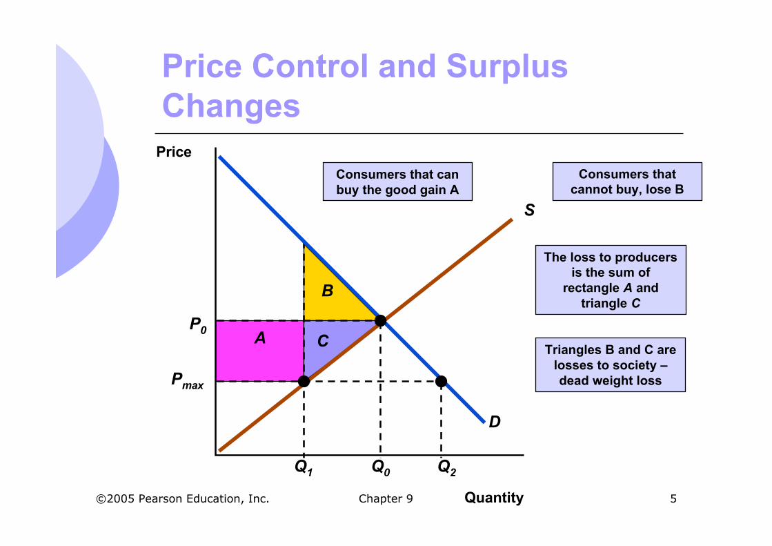
The loss to producersis the sum of
rectangle A andtriangle C
B
A C
Consumers that canbuy the good gain A
Price Control and SurplusChanges
Quantity
Price
S
D
P0
Q0
Pmax
Q1 Q2
Consumers thatcannot buy, lose B
Triangles B and C arelosses to society –dead weight loss

Chapter 9 6©2005 Pearson Education, Inc.
Price Controls and WelfareEffects
� The total loss is equal to area B + C
� The deadweight loss is the inefficiencyof the price controls – the total loss insurplus (consumer plus producer)
Chapter 9 7©2005 Pearson Education, Inc.
Price Controls andNatural Gas Shortages
� From example in Chapter 2, 1975 Pricecontrols created a shortage of naturalgas
�What was the effect of those controls?�Decreases in surplus and overall loss for
society
�We can measure these welfare effects fromthe demand and supply of natural gas

Chapter 9 8©2005 Pearson Education, Inc.
Price Controls andNatural Gas Shortages
�QS = 14 + 2PG + 0.25PO
�Quantity supplied in trillion cubic feet (Tcf)
�QD = -5PG + 3.75PO
�Quantity demanded (Tcf)
�PG = price of natural gas in $/thousandcubic feet (mcf)
�PO = price of oil in $/barrel

Chapter 9 9©2005 Pearson Education, Inc.
Price Controls andNatural Gas Shortages
�Using PO = $8/b and givesequilibrium values for natural gas�PG = $2/mcf and QG = 20 Tcf
�Price ceiling was set at $1/mcf
�Showing this graphically, we can see andmeasure the effects on producer andconsumer surplus
GS
GD QQ =

Chapter 9 10©2005 Pearson Education, Inc.
B
A
C
The gain to consumersis
rectangle A minustriangle B, and the loss
to producers isrectangle A plus
triangle C.
SD
2.00
2.40
Price($/mcf)
Quantity (Tcf)0 5 10 15 20 25 3018
(Pmax)1.00
Price Controls andNatural Gas Shortages
Chapter 9 11©2005 Pearson Education, Inc.
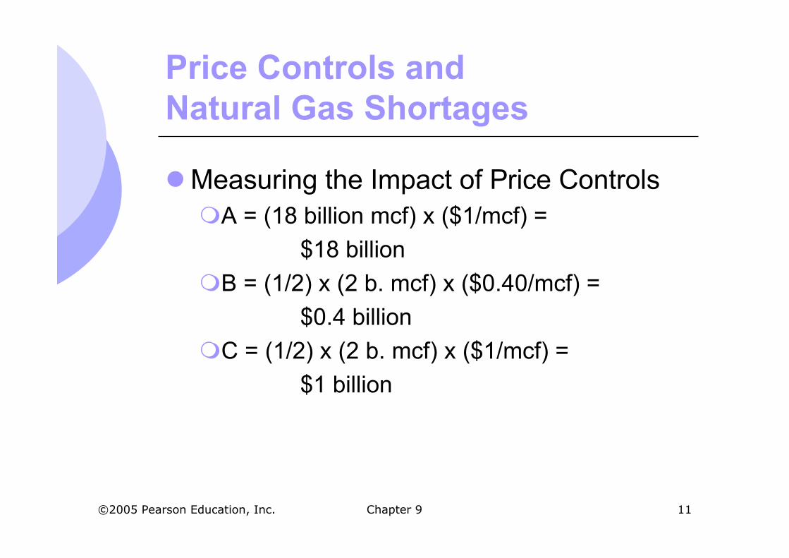
Price Controls andNatural Gas Shortages
�Measuring the Impact of Price Controls�A = (18 billion mcf) x ($1/mcf) =
$18 billion
�B = (1/2) x (2 b. mcf) x ($0.40/mcf) =
$0.4 billion
�C = (1/2) x (2 b. mcf) x ($1/mcf) =
$1 billion

Chapter 9 12©2005 Pearson Education, Inc.
Price Controls andNatural Gas Shortages
�Measuring the Impact of Price Controls in1975 (You may want to check byyourself.)�Change in consumer surplus
� = A - B = 18 - 0.4 = $17.6 billion Gain
�Change in producer surplus� = A + C = 18 + 1 = $19.0 billion Loss
�Dead Weight Loss� = B + C = 0.4 + 1 = $1.4 billion Loss

Chapter 9 13©2005 Pearson Education, Inc.
The Efficiency ofa Competitive Market
� In the evaluation of markets, we often talkabout whether it reaches economicefficiency�Maximization of aggregate consumer and
producer surplus
�Policies such as price controls that causedead weight losses in society are said toimpose an efficiency cost on theeconomy
Chapter 9 14©2005 Pearson Education, Inc.
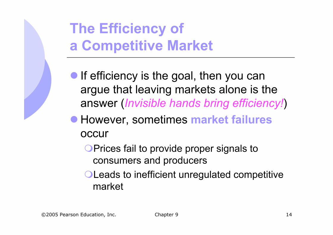
The Efficiency ofa Competitive Market
� If efficiency is the goal, then you canargue that leaving markets alone is theanswer (Invisible hands bring efficiency!)
�However, sometimes market failuresoccur�Prices fail to provide proper signals to
consumers and producers
�Leads to inefficient unregulated competitivemarket

Chapter 9 15©2005 Pearson Education, Inc.
Types of Market Failures
1. Externalities� Costs or benefits that do not show up as part of the
market price (e.g. pollution, elementary education)� Costs or benefits are external to the market
2. Lack of Information� Imperfect information prevents consumers from
making utility-maximizing decisions
� Government intervention may be desirable inthese cases---e.g., imposing emissionregulations, compulsory education
Chapter 9 16©2005 Pearson Education, Inc.
The Efficiency of a CompetitiveMarket
�Other than market failures, unregulatedcompetitive markets lead to economicefficiency

Chapter 9 17©2005 Pearson Education, Inc.
The Market for Human Kidneys(pp. 307-9)
� The 1984 National Organ TransplantationAct prohibits the sale of organs fortransplantation
�What has been the impact of the Act?�We can measure this using the supply
and demand for kidneys from estimateddata (P: the price of a kidney)�Supply: QS = 8,000 + 0.2P�Demand: QD = 16,000 - 0.2P
Chapter 9 18©2005 Pearson Education, Inc.
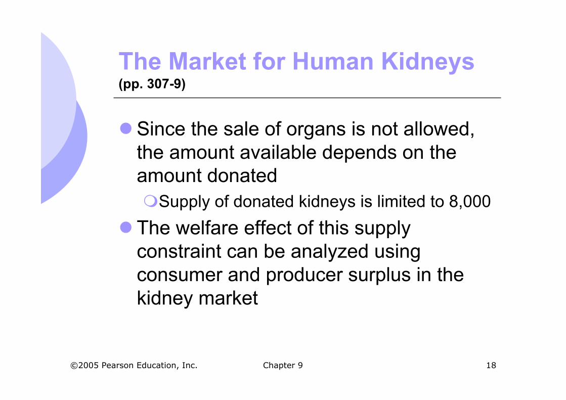
The Market for Human Kidneys(pp. 307-9)
�Since the sale of organs is not allowed,the amount available depends on theamount donated�Supply of donated kidneys is limited to 8,000
� The welfare effect of this supplyconstraint can be analyzed usingconsumer and producer surplus in thekidney market
Chapter 9 19©2005 Pearson Education, Inc.
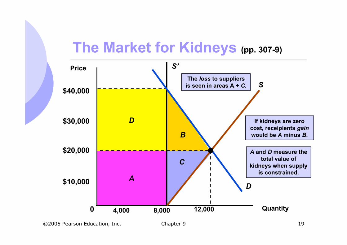
D
A and D measure thetotal value of
kidneys when supplyis constrained.
A
C
The loss to suppliersis seen in areas A + C.
The Market for Kidneys (pp. 307-9)
Quantity
Price
4,0000
$10,000
$30,000
$40,000
8,000
S’
B
If kidneys are zerocost, receipients gainwould be A minus B.
S
D
12,000
$20,000

Chapter 9 20©2005 Pearson Education, Inc.
The Market for Human Kidneys(pp. 307-9)
�Suppliers:�Those who supply them are not paid the
market price, estimated at $20,000� Loss of surplus equal to area A = $160 million
�Some who would donate for the equilibriumprice do not donate in the current market� Loss of surplus equal to area C = $40 million
�Total loss of A + C in producers’ surplus =$200 million
Chapter 9 21©2005 Pearson Education, Inc.
The Market for Human Kidneys(pp. 307-9)
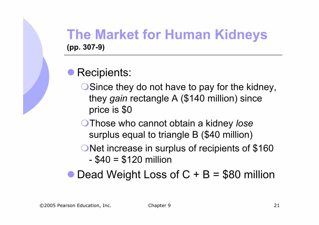
�Recipients:�Since they do not have to pay for the kidney,
they gain rectangle A ($140 million) sinceprice is $0
�Those who cannot obtain a kidney losesurplus equal to triangle B ($40 million)
�Net increase in surplus of recipients of $160- $40 = $120 million
�Dead Weight Loss of C + B = $80 million

Chapter 9 22©2005 Pearson Education, Inc.
The Market for Human Kidneys(pp. 307-9)
�Other Inefficiency Costs�Allocation is not necessarily to those who
value the kidneys the most
�Price may increase to $40,000, theequilibrium price, with hospitals getting theprice
Chapter 9 23©2005 Pearson Education, Inc.
The Market for Human Kidneys(pp. 307-9)
� Arguments in favor of prohibiting thesale of organs:
1. Imperfect information about donor’s healthand screening
2. Unfair to allocate according to the ability topay� Holding price below equilibrium will create
shortages
� Organs versus artificial substitutes

Chapter 9 24©2005 Pearson Education, Inc.
Minimum Prices
�Periodically, government policy seeks toraise prices above market-clearing levels�Minimum wage law
�Regulation of airlines
�Agricultural policies
�We will investigate this by looking at theminimum wage legislation

Chapter 9 25©2005 Pearson Education, Inc.
Minimum Prices
�When price is set above the marketclearing price:�Quantity demanded falls
�Suppliers may, however, choose to increasequantity supplied in face of higher prices
�This causes additional producer losses equalto the total cost of production above quantitydemanded
Chapter 9 26©2005 Pearson Education, Inc.
BA
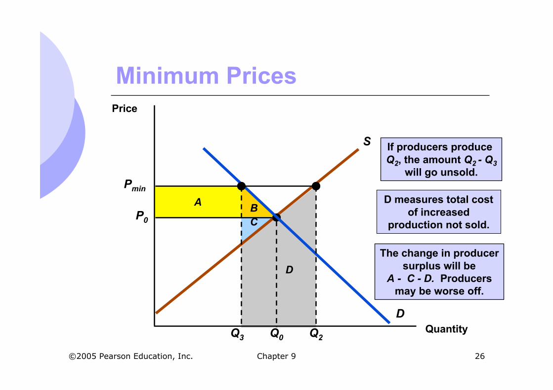
The change in producersurplus will be
A - C - D. Producersmay be worse off.
C
D
Minimum Prices
Quantity
Price
S
D
P0
Q0Q3 Q2
Pmin
If producers produce Q2, the amount Q2 - Q3
will go unsold.
D measures total costof increased
production not sold.

Chapter 9 27©2005 Pearson Education, Inc.
Minimum Prices
� Losses in consumer surplus are still thesame [-(A+B)]�Increased price leading to decreased
quantity equals area A
�Those priced out of the market lose area B
�Producer surplus similar�Increases from increased price for units sold
equal to A
�Losses from drop in sales equal to C

Chapter 9 28©2005 Pearson Education, Inc.
Minimum Prices
�What if producers expand production toQ2 from the increased price?�Since they only sell Q3, there is no revenue
to cover the additional production (Q2-Q3)
�Supply curve measures MC of production sototal cost of additional production is areaunder the supply curve for the increasedproduction (Q2-Q3) = area D
�Total change in producer surplus = A – C – D

Chapter 9 29©2005 Pearson Education, Inc.
Minimum Wages
�Wage is set higher than market clearingwage
�Decreased quantity of workersdemanded
� Those workers hired receive higherwages
�Unemployment results, since noteveryone who wants to work at the newwage can

Chapter 9 30©2005 Pearson Education, Inc.
B
The deadweight lossis given by
triangles B and C.
C
A
L1 L2
Unemployment
wmin
Firms are not allowed topay less than wmin. This
results in unemployment.
S
D
w0
L0
The Minimum Wage
L
w
A is gain to workerswho find jobs at
higher wage.

Chapter 9 31©2005 Pearson Education, Inc.
Airline Regulation
�Before 1970, the airline industry washeavily regulated by the Civil AeronauticsBoard (CAB)
�During 1976-1981, the airline industry inthe U.S. changed dramatically asderegulation led to major changes
�Some airlines merged or went out ofbusiness as new airlines entered theindustry
Chapter 9 32©2005 Pearson Education, Inc.
Airline Regulation
�Although prices in the industry fellconsiderably (helping consumers), profitsdid not.�Regulation caused significant inefficiencies
and artificially high costs
�We can show the effects of thisregulation by looking at the effects onsurplus from the controlled prices

Chapter 9 33©2005 Pearson Education, Inc.
BA
C
After deregulation:Prices fell to PO. Thechange in consumer
surplus is A + B.
Q3
D
Area D is the costof unsold output.
Effect of Airline Regulation
Quantity
Price S
D
P0
Q0Q1
Pmin
Q2
Prior to deregulationprice was at Pmin.
Production was Q3hoping to outsell
competitors.

Chapter 9 34©2005 Pearson Education, Inc.
Airline Industry Data

Chapter 9 35©2005 Pearson Education, Inc.
Airline Industry Data
� Airline industry data show:1. Long-run adjustment as the number of
carriers increased and prices decreased
2. Higher load factors indicating moreefficiency
3. Falling rates
4. Real cost increased slightly (adjusted fuelcost)
5. Large welfare gain

Chapter 9 36©2005 Pearson Education, Inc.
Effect of Airline Regulation
1. Large welfare gain
Consumers’ gain=A+B
Producers’ gain=C+D-A
Net welfare gain=B+C+D