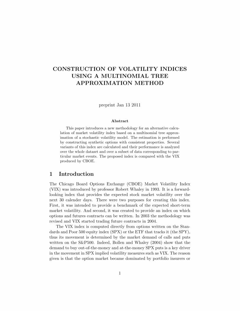
CONSTRUCTION OF VOLATILITY INDICESUSING A MULTINOMIAL TREE

APPROXIMATION METHOD

preprint Jan 13 2011

Abstract

This paper introduces a new methodology for an alternative calcu-lation of market volatility index based on a multinomial tree approx-imation of a stochastic volatility model. The estimation is performedby constructing synthetic options with consistent properties. Severalvariants of this index are calculated and their performance is analyzedover the whole dataset and over a subset of data corresponding to par-ticular market events. The proposed index is compared with the VIXproduced by CBOE.

1 Introduction

The Chicago Board Options Exchange (CBOE) Market Volatility Index(VIX) was introduced by professor Robert Whaley in 1993. It is a forward-looking index that provides the expected stock market volatility over thenext 30 calender days. There were two purposes for creating this index.First, it was intended to provide a benchmark of the expected short-termmarket volatility. And second, it was created to provide an index on whichoptions and futures contracts can be written. In 2003 the methodology wasrevised and VIX started trading future contracts in 2004.

The VIX index is computed directly from options written on the Stan-dards and Poor 500 equity index (SPX) or the ETF that tracks it (the SPY),thus its movement is determined by the market demand of calls and putswritten on the S&P500. Indeed, Bollen and Whaley (2004) show that thedemand to buy out-of-the-money and at-the-money SPX puts is a key driverin the movement in SPX implied volatility measures such as VIX. The reasongiven is that the option market became dominated by portfolio insurers or

1

hedgers, who routinely buy out-of-the-money and at-the-money SPX indexput options for insurance purposes to protect their portfolio from a poten-tial market crash. Very often, the VIX index was termed as an “InvestorFear Gauge”. This is due to the fact that the VIX spikes during periods ofmarket turmoil.

1.1 Calculation of VIX by CBOE

The current calculation of VIX by CBOE is based on the concept of fairvalue of future variance developed by Demeterfi et al. (1999). The fair valueof future variance is determined from market observables such as optionprices and interest rates independent of any option pricing model. The fairvalue of future variance is defined as following (equation 26 in Demeterfiet al. (1999)):

Kvar =2

T

{rT −

[S0

S∗erT − 1

]− log

(S∗S0

)+ erT

∫ S∗

0

P (T,K)

K2dK

+ erT∫ ∞S∗

C(T,K)

K2dK

}(1)

where S0 is the current asset price, C and P are call and put prices, respec-tively, r is the risk-free rate, T and K are option maturity and strike price,respectively, and S∗ is an arbitrary stock price which is typically chosen tobe close to the forward price.

The calculation of VIX by CBOE follows equation (1), as explained inthe CBOE white paper (see CBOE (2003)). CBOE calculates the VIX indexusing the following formula:

σ2vix =

2

T

∑i

∆Ki

K2i

erTQ(T,Ki)−1

T

(F0

K0− 1

)2

(2)

where

• σvix is the V IX100 .

• T is the time to expiration.

• F0 is the forward index level derived from index option prices.

• Ki is the ith out-of-money option; a call if Ki > F0 and a put ifKi < F0.

2

• ∆Ki is the inverval between strike prices-half the distance between thestrike on either side of ,Ki:

∆Ki =Ki+1 −Ki−1

2(3)

Please note that ∆K for the lowest or highest strike is simply thedifference between the the lowest or highest strike and the next strikeprice.

• K0 is the first strike below the forward index level.

• r is the risk-free interest rate to expiration.

• And Q(T,Ki) is the mid point of the bid-ask spread of each optionwith strike Ki.

A step by step calculation and an example that replicates the value ofthe VIX for a particular day is provided in the Appendix A.

1.2 Issues with CBOE Procedure for VIX Calculation

As shown by Jiang and Tian (2007), there are differences between the fairvalue of future variance and the practical implementation of VIX providedby CBOE. The main differences come from the following:

(1) The calculation of fair value of future variance uses continuous strikeprices. However, strike price vectors on CBOE or any other exchangeare generally discrete.

(2) The calculation of fair value of future variance uses strike prices be-tween 0 and ∞. But in reality, the strike prices have a small range.

(3) The fair value of future variance produce the expected variance (volatil-ity) corresponding to the maturity date of the options used. In reality,options with exact 30-day maturity are not available. VIX is obtainedby linearly interpolating the variances of options with near term andnext term maturity.

Due to the truncation of the data and the discreteness of the data, theCBOE procedure can generate errors (Jiang and Tian, 2007).

3

2 New Methodology

2.1 Theoretical frame of stochastic volatility quadrinomialtree method

Stochastic volatility models have been proposed to better model the com-plexity of the market. The quadrinomial tree approximation developed byFlorescu and Viens (2008) has demonstrated that it can be used to estimateoption values and that it produces option chain values which are within bidask spread. The quadrinomial tree method outperforms other approximat-ing techniques (with the exception of analytical solutions) in terms of botherror and time. In this work we use this methodology to approximate anunderlying asset price process following:

dXt =

(r − ϕ2

t

2

)dt+ ϕtStdWt, (4)

where Xt = logSt and St is the asset price, r is the short-term risk-freerate of interest, Wt a standard Brownian Motions. ϕt models the stochasticvolatility process. It has been proved that for any proxy of the currentstochastic volatility distribution at t the option prices calculated at timet converge to the true option prices (Theorem 4.6 in Florescu and Viens(2008)).

When using Stochastic volatility models we are faced with a real problemwhen trying to come up with ONE number describing the volatility. Themodel intrinsically has an entire distribution describing the volatility andtherefore providing a number is nonsensical. However, since a number weneed to provide the idea of this approach is to produce the price of a syntheticone month option with strike exactly the spot price and calculate the impliedvolatility value corresponding to the price we produce. The real challengeis to come up with a stochastic volatility distribution characteristic to thecurrent market conditions.

In the current work we take the simplest approach possible. We usea proxy for this ϕt calculated directly from the implied volatility valuescharacterizing the option chains. This is used in conjunction with a highlyrecombining quadrinomial tree method to compute the price of options.The quadrinomial tree method is described in details in Florescu and Viens(2008). In the Appendix B we describe a one-step quadrinomial tree con-struction.

4

2.2 Difference between CBOE Procedure and QuadrinomialTree Method

(1) CBOE procedure calculates two variances from near term and nextterm out-of-money options chains and then it obtains the expectedvariance in 30-day by linearly interpolating the variance from nearterm and next term options chain. This arbitrary linear interpolationlacks a theoretical base. Using the quadrinomial tree method, we cancompute the expected market volatility in exactly 30 days.

(2) Criteria for selection of the options used for the calculation are differ-ent. In CBOE procedure, the out-of-money options are first arrangedaccording to the increase in strike price. All the individual optionsin the near term and next term out-of-money options are selected aslong as two options next to each other don’t have zero price at thesame time. However, in our analysis we observe that some of the op-tions selected are not actively traded and therefore their price maynot reflect the expectation of the current market conditions. In thequadrinomial tree method, we select all the options (regardless of be-ing out-of-money or not) as long as they reflect the market volatility.This is ensured by selecting all options with volume higher than 0.

(3) In the CBOE procedure, 8 days before the maturity of the near termoptions chain, CBOE will roll over to the next/third options chains.The argument is that when the options are close to maturity, theirprice is more volatile and thus cannot represent the market volatility.However, it is also well known that options with larger maturities tendsto have volatility close to the long term market mean volatility and thiscan lead to underestimating the market volatility. In the quadrinomialtree method, we use all the data of near term and next term optionschains.

(4) In this work, we use all relevant options weighted accordingly. In the-ory all options with different maturities may be incorporated as theyreflect the market volatility. Only the near term and next term op-tions chains are used in this work, as from empirical studies includingoptions with longer maturities have associated little weight and theydo not generally influence the final result.

5

3 Results and Discussions

3.1 Constructing a volatility index using different inputs

Options written on S&P500 have three near term expiration months followedby three additional expiration months from the March quarterly cycle. Wenote that for the VIX calculation by CBOE, the closest near term optionschain and the next term options chain are used. Also, when the maturityof the near term options is less than 8 days, next term options and theones after will be used in the calculation. For the quadrinomial tree model,we explore the effects of using different option types and maturity on theresulting volatility index. In the next figures we compare constructed indicesusing five different ways.

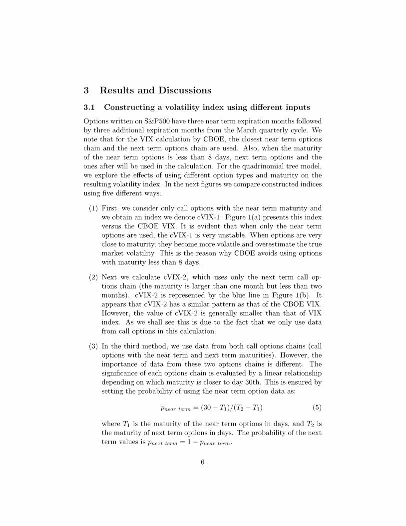
(1) First, we consider only call options with the near term maturity andwe obtain an index we denote cVIX-1. Figure 1(a) presents this indexversus the CBOE VIX. It is evident that when only the near termoptions are used, the cVIX-1 is very unstable. When options are veryclose to maturity, they become more volatile and overestimate the truemarket volatility. This is the reason why CBOE avoids using optionswith maturity less than 8 days.

(2) Next we calculate cVIX-2, which uses only the next term call op-tions chain (the maturity is larger than one month but less than twomonths). cVIX-2 is represented by the blue line in Figure 1(b). Itappears that cVIX-2 has a similar pattern as that of the CBOE VIX.However, the value of cVIX-2 is generally smaller than that of VIXindex. As we shall see this is due to the fact that we only use datafrom call options in this calculation.

(3) In the third method, we use data from both call options chains (calloptions with the near term and next term maturities). However, theimportance of data from these two options chains is different. Thesignificance of each options chain is evaluated by a linear relationshipdepending on which maturity is closer to day 30th. This is ensured bysetting the probability of using the near term option data as:

pnear term = (30− T1)/(T2 − T1) (5)

where T1 is the maturity of the near term options in days, and T2 isthe maturity of next term options in days. The probability of the nextterm values is pnext term = 1− pnear term.

6

Figure 1: Comparison of VIX constructed using different methods: (a)cVIX-1 which is computed from actively traded call options with the near-est maturity; (b) cVIX-2 (computed from actively traded call options withmore than one-month but less than two-month maturity) and cVIX-b (con-structed using call options with less than two-month maturity).

7

The index obtained by this method is denoted with cVIX-b and isshown in Figure 1(b) by the red line. We note that the cVIX-b hasa similar pattern as the CBOE VIX. Similarly with the cVIX-2, thevalues are generally lower than the VIX. When comparing cVIX-b tocVIX-2, due to the effect of incorporation more volatile data, occa-sionally cVIX-b has higher value than cVIX-2, especially when thereis a spike in the VIX value.

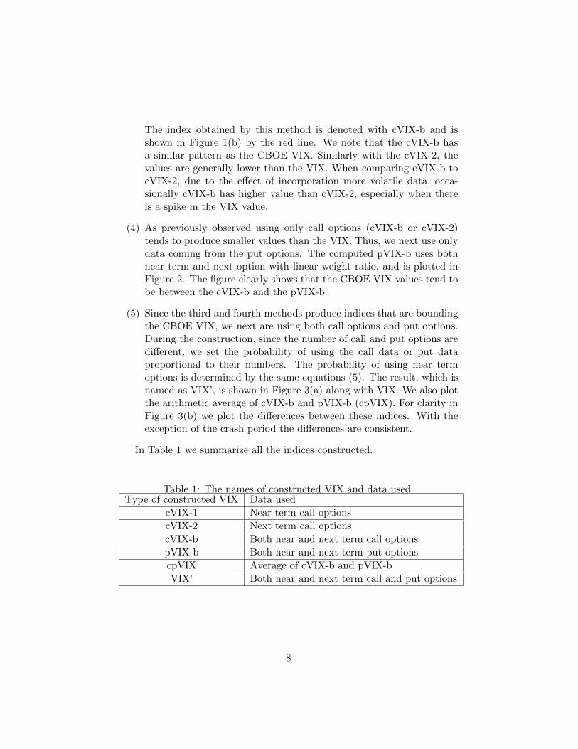
(4) As previously observed using only call options (cVIX-b or cVIX-2)tends to produce smaller values than the VIX. Thus, we next use onlydata coming from the put options. The computed pVIX-b uses bothnear term and next option with linear weight ratio, and is plotted inFigure 2. The figure clearly shows that the CBOE VIX values tend tobe between the cVIX-b and the pVIX-b.

(5) Since the third and fourth methods produce indices that are boundingthe CBOE VIX, we next are using both call options and put options.During the construction, since the number of call and put options aredifferent, we set the probability of using the call data or put dataproportional to their numbers. The probability of using near termoptions is determined by the same equations (5). The result, which isnamed as VIX’, is shown in Figure 3(a) along with VIX. We also plotthe arithmetic average of cVIX-b and pVIX-b (cpVIX). For clarity inFigure 3(b) we plot the differences between these indices. With theexception of the crash period the differences are consistent.

In Table 1 we summarize all the indices constructed.

Table 1: The names of constructed VIX and data used.Type of constructed VIX Data used

cVIX-1 Near term call options

cVIX-2 Next term call options

cVIX-b Both near and next term call options

pVIX-b Both near and next term put options

cpVIX Average of cVIX-b and pVIX-b

VIX’ Both near and next term call and put options

8

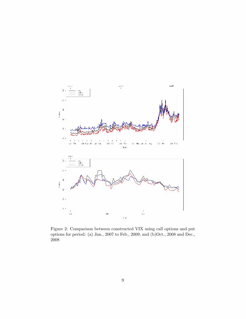
Figure 2: Comparison between constructed VIX using call options and putoptions for period: (a) Jan., 2007 to Feb., 2009; and (b)Oct., 2008 and Dec.,2008

9

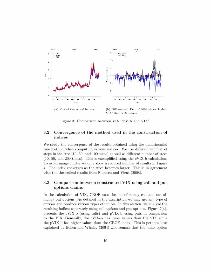
(a) Plot of the actual indices (b) Differences. End of 2009 shows higherVIX’ than VIX values

Figure 3: Comparison between VIX, cpVIX and VIX’

3.2 Convergence of the method used in the construction ofindices

We study the convergence of the results obtained using the quadrinomialtree method when computing various indices. We use different number ofsteps in the tree (10, 50, and 100 steps) as well as different number of trees(10, 50, and 200 times). This is exemplified using the cVIX-b calculation.To avoid image clutter we only show a reduced number of results in Figure4. The index converges as the trees becomes larger. This is in agreementwith the theoretical results from Florescu and Viens (2008).

3.3 Comparison between constructed VIX using call and putoptions chains

In the calculation of VIX, CBOE uses the out-of-money call and out-of-money put options. As detailed in the description we may use any type ofoptions and produce various types of indices. In this section, we analyze theresulting indices separately using call options and put options. Figure 2(a),presents the cVIX-b (using calls) and pVIX-b using puts in comparisonto the VIX. Generally, the cVIX-b has lower values than the VIX whilethe pVIX-b has higher values than the CBOE index. This is perhaps bestexplained by Bollen and Whaley (2004) who remark that the index option

10

Figure 4: Convergence of constructed volatility index using quadrinomialtree method

market such as S&P500 became dominated by portfolio insurers or hedgers,who routinely buy out-of-the-money and at-the-money SPX put options forinsurance purposes. This drives up the price of put options and therefore theimplied volatilities from put options tends to be higher. This leads to thedifferences between the constructed VIX using call options and put options.

In Figure 2(b) we zoom into turbulent financial time between Oct. andDec. 2008. It is clear that during this period, the VIX is generally thehigher than either cVIX or pVIX. This seem to indicate us that during thisperiod the demand for put options seems to be extraordinary. We shouldalso note that during this period of time, the market was very volatile andthe observed VIX index went as high as 80. Furthermore, when lookingat the difference between the call based index (cVIX-b) and the put basedindex (pVIX-b) the spread between these volatilities was the smallest forthis particular period. In Figure 5 we showcase this feature and we observethat the spread becomes negative before the market crash and stays negativefor an extended period during the crash.

11

Figure 5: The difference (spread) pVIX-cVIX. A decrease in spread seemsto indicate a decrease in the market index

12

3.4 A comparison of the correlation between the constructedindices/S&P500 and VIX/S&P500

It is well documented that a negative relationship exists between the indexS&P500 and the CBOE volatility index VIX; when the S&P500 index goesup/down, VIX tends to go down/up. In Table 2, we present the R2 of thelinear relationship between S&P500 and various indices. The data does notshow major differences between these correlations.

Table 2: The correlation between constructed VIX or VIX to S&P500.sp500 VIX cVIX-2 cVIX-b pVIX-2 pVIX-b cpVIX-b cpVIX-2

R2 0.7818 0.7944 0.7805 0.7875 0.7912 0.8004 0.8030

3.5 An analysis of the predictive power of the different in-dices

In this section we analyze the relationship between the volatility and thereturn of the S&P500. Specifically, we are interested in determining whethera significant increase in the volatility is followed by a significant drop in theS&P500 prices and to determine which volatility index variant prove to be abetter predictor of this relationship. We analyze the same day observationsas well as one day forecast. Furthermore, we investigate the relationshipfor a selection of observations centered around major financial events aspresented in Table 3. We consider the VIX from CBOE and the followingindex variants: cpVIX, VIX’, cVIXb, and pVIXb.

For each of these variants we calculate the rate of change and we estimatethe conditional probability that S&P500 is moving in the opposite direction.

Prob(ReturnS&P500 < 0 | (ReturnVol Index > L, lag = d)), and (6)

Prob(ReturnS&P500 > 0 | (ReturnVol Index < L, lag = d))

where ReturnS&P500 is the return of S&P500, ReturnVol Index is the returnof the particular volatility index, L is a threshold for the index return, andd represents the same day for d = 0, and the previous day for d = 1.

The graphs presented are grouped in two sections corresponding to thesame day d = 0 or the forecast for the next day d = 1. On all of these graphsthe x-axis plots the respective threshold that conditions the probabilities in

13

Figure 6: Probability of a positive return on S&P500 when d = 0

Figure 7: Probability of a negative return on S&P500 when d = 0

14

(6) while the y axis plots the percent of days where the S&P500 moved inthe predicted direction. The left image in a figure presents all the dataset,while the right image is restricted to the important financial events detailedin Table 3 on page 16.

15

Table 3: Important events that happened during Jan 07 to Feb 09 period.Central banks increase money supply Aug. 10, 2007Countywide job slashes Sep. 7, 2007Bush calls for economic stimulus package Jan. 18, 2008Central European banks plan emergency cash infusion Mar. 11, 2008Bear Stearns gets emergency funds Mar.14, 2008J.P.Morgan to acquire Bear Stearns Mar. 16, 2008Federal Reserve cuts rates by 0.75 Mar. 18, 2008IMF may sell 400 tons of gold Apr. 8, 2008Citigroup anticipates a giant loss, Fed cuts rate again Apr. 30, 2008US backs lending firms Jul. 13, 2008US inflation at 26 year high Jul. 16, 2008Mortgage firms bail out Sep. 7, 2008Lehman Brothers files for bankruptcy Sep. 14, 2008Bush hails the financial rescue plan Sep. 19, 2008$700 billion package failed Sep. 29, 2008House backs the bail out plan Oct. 3, 2008plans to buy 125 billion stakes in banks Oct. 14-29, 2008Citigroup cut 75000 jobs Nov. 17, 2008Citigroup gets US Treasury lifeline Nov. 23, 2008800 billion stimulus package announced Nov.25, 2008Bank of America cuts 30000 jobs Dec. 11, 2008Madoff 50 billion scandal Dec. 13, 2008Auto industry bail-out Dec. 19, 2009US financial sector stocks decline sharply Jan. 20, 2009New bank bail-out Feb. 10, 2009

We analyze separately the positive and negative movement in figures 6and 7. It is pretty clear from these images that the CBOE VIX is the bestindicator for the return/volatility evolution within the same day (d = 0).The profile of the probability curves for the major events selection followsa similar profile to the probability curves for all data analyzed. However,the fact that an increase in the volatility index calculated from the callsindicates a drop in the S&P500 index was a surprise to us.

For prediction purposes, we analyze the relationship between the previ-ous day volatility index and the return on the S&P500 the following day.The corresponding graphs once again split by the positive and negative

16

Figure 8: Probability of a positive return on S&P500 when d = 1

thresholds are presented in figures 8 respectively 9.This time we observe that the CBOE VIX is one of the worst indicators

for future day evolution of the S&P500. In some cases the probability ofpredicting a positive return correctly is well below 50%.

In contrast two of the indices we calculated stand out. We note that adrop in the cVIXb (calculated from call options) forecasts with the highestprobability a positive return of the S&P500. Furthermore, an increase in thepVIXb (calculated from the put options) has a clear advantage in forecastingsecond day negative S&P500 returns. The probabilities for the pVIXb arein fact very high for all data sample and also for the major events in themarket considered in this analysis.

We hope that we convinced the reader that using different types of op-tions in the volatility index calculation has the potential to reveal moreinformation about the market than the VIX.

4 Summary and Conclusion

We propose a new methodology of calculating a value that represents themarket volatility at a given moment in time by implementing a stochasticvolatility technique. We believe this technique is a viable way to producea market index. We propose several variants of such indices and we believeeach of them is valuable as an indicator of a market movement. The in-dex constructed from calls (cVIX-b) may be considered as an indicator of

17

Figure 9: Probability of a negative return on S&P500 when d = 1

market’s positive movement while the index constructed from put options(pVIX-b) as an indicator of future negative movement in the market. Thedifference (spread) between the two indices may be indicative of future mar-ket movement. The average of these two indices (cpVIX) and the indexconstructed with all options (VIX’) both have value in determining whenthe VIX undervalues or overvalues the market volatility.

Finally, we analyze the relations between all these types of indices. Webelieve all of them bring more information about the market and the method-ology has the potential to produce market indicators each indicative of acertain aspect of the financial market.

Appendix A: Step-by-Step Explanation of the CBOEProcedure for Calculating VIX Index

Using data obtained at the market close on Sept 8, 2009, we replicate theVIX value following the CBOE procedure. First, we need to do some calcu-lation and re-arrangement of the data. The procedure is described below.

1. Selection of options chains. VIX generally uses put and call options inthe two nearest-term expiration months while there are more optionschains trading in the market. Also, it should be pointed out that,with 8 days left to expiration, the VIX “rolls” to the second and thirdcontract months in order to minimize the pricing anomalies that might

18

occur close to the maturity.

2. T , the time to expiration, is measured in minutes rather than in days.Specifically, the calculation of T is given by the following expression:

T = {Mcurrentday +Msettlementday +Motherdays}/Myear (7)

Where:Mcurrentday is the number of minutes remaining until midnight of thecurrent day, Msettlementday is the number of minutes from midnightuntil 8:30 a.m. on SPX settlement day, and Motherdays is the numberof minutes in all the days between current day and the settlement day,and Myear is the number of minutes in a year.

3. Calculating the at-the-money strike. This is done by finding the strikeprice at which the difference between the call and put prices is thesmallest.

4. Calculation of F , the forward index level. This is based on the pre-viously determined at-the-money option prices and the correspondingstrike price:

F = StrikePrice+ erT (CallPrice− PutPrice) (8)

Note that since two options chains are used in the calculation, twoforward index level should be obtained, for the near term and nextterm options chains.

5. Selection of K0, the strike price immediately below the forward indexlevel, F .

In the following, we demonstrate how to obtain the VIX value usingCBOE procedure using data obtained when the S&500 options stopped trad-ing at 3:15PM (Middle time) on Sept 8, 2009.

Step 1: Calculate the time to expiration T , forward index level F , K0, thestrike price immediately below F , and data arrangement:T1 = {Mcurrentday +Msettlementday +Motherdays}/Myear

= (525 + 510 + 12960)/525600= 0.026626712T2 = {Mcurrentday +Msettlementday +Motherdays}/Myear

= (525 + 510 + 53280)/525600= 0.103339041

19

We should note that the total days in a year is 365 days. Since thesmallest difference between call and put price is at strike $1025, theat-the-money strike is determined to be at $1025 for both near termoptions and next term options. Therefore, using federal funds effectiverate at 0.15%, the forward index level F1 for the near term options andforward index level F2 for the next term options are:F1 = StrikePrice+ erT1(CallPrice− PutPrice)= 1025 + e0.0015×0.026626712(13.25− 13.9) = 1024.35F2 = StrikePrice+ erT2(CallPrice− PutPrice)= 1025 + e0.0015×0.103339041(29.15− 30.35) = 1023.80

We also obtain K0, the strike price immediately below F , which is$1020 for both expirations. Then we select call and put options thathave strike prices greater and smaller, respectively, than K0 (it is 1020here) and non-zero bid price. After encountering two consecutive op-tions with a bid price of zero, do not select any other options. Notethat the prices of the options are calculated using the midpoint of thebid-ask spread. At K0, the average of call and put price is used. Thedata selected is summarized below:

• Calculation of time to maturity:T1 = 0.026626712T2 = 0.103339041

• At-the-money strike: $1025 for both near term options and nextterm options.

• Federal funds effective rate: 0.15%.

• The forward index level F1 for the near term options and forwardindex level F2 for the next term options are:F1 = 1024.35F2 = 1023.80

• K0, the strike price immediately below F , is $1020 for both ex-pirations.

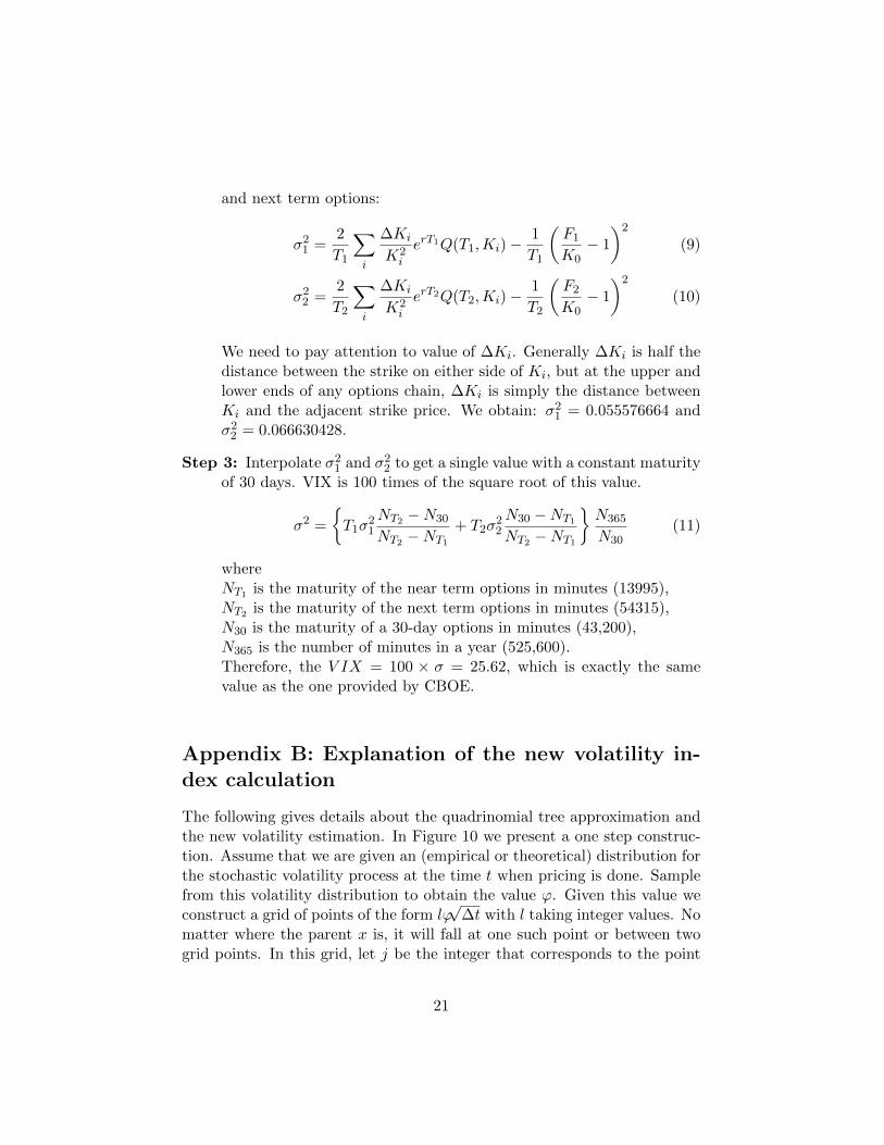
Step 2: Calculate the volatility for near term and next term options. Weapply the following equations to calculate the VIX to the near term

20

and next term options:

σ21 =

2

T1

∑i

∆Ki

K2i

erT1Q(T1,Ki)−1

T1

(F1

K0− 1

)2

(9)

σ22 =

2

T2

∑i

∆Ki

K2i

erT2Q(T2,Ki)−1

T2

(F2

K0− 1

)2

(10)

We need to pay attention to value of ∆Ki. Generally ∆Ki is half thedistance between the strike on either side of Ki, but at the upper andlower ends of any options chain, ∆Ki is simply the distance betweenKi and the adjacent strike price. We obtain: σ2

1 = 0.055576664 andσ2

2 = 0.066630428.

Step 3: Interpolate σ21 and σ2

2 to get a single value with a constant maturityof 30 days. VIX is 100 times of the square root of this value.

σ2 =

{T1σ

21

NT2 −N30

NT2 −NT1

+ T2σ22

N30 −NT1

NT2 −NT1

}N365

N30(11)

whereNT1 is the maturity of the near term options in minutes (13995),NT2 is the maturity of the next term options in minutes (54315),N30 is the maturity of a 30-day options in minutes (43,200),N365 is the number of minutes in a year (525,600).Therefore, the V IX = 100 × σ = 25.62, which is exactly the samevalue as the one provided by CBOE.

Appendix B: Explanation of the new volatility in-dex calculation

The following gives details about the quadrinomial tree approximation andthe new volatility estimation. In Figure 10 we present a one step construc-tion. Assume that we are given an (empirical or theoretical) distribution forthe stochastic volatility process at the time t when pricing is done. Samplefrom this volatility distribution to obtain the value ϕ. Given this value weconstruct a grid of points of the form lϕ

√∆t with l taking integer values. No

matter where the parent x is, it will fall at one such point or between twogrid points. In this grid, let j be the integer that corresponds to the point

21

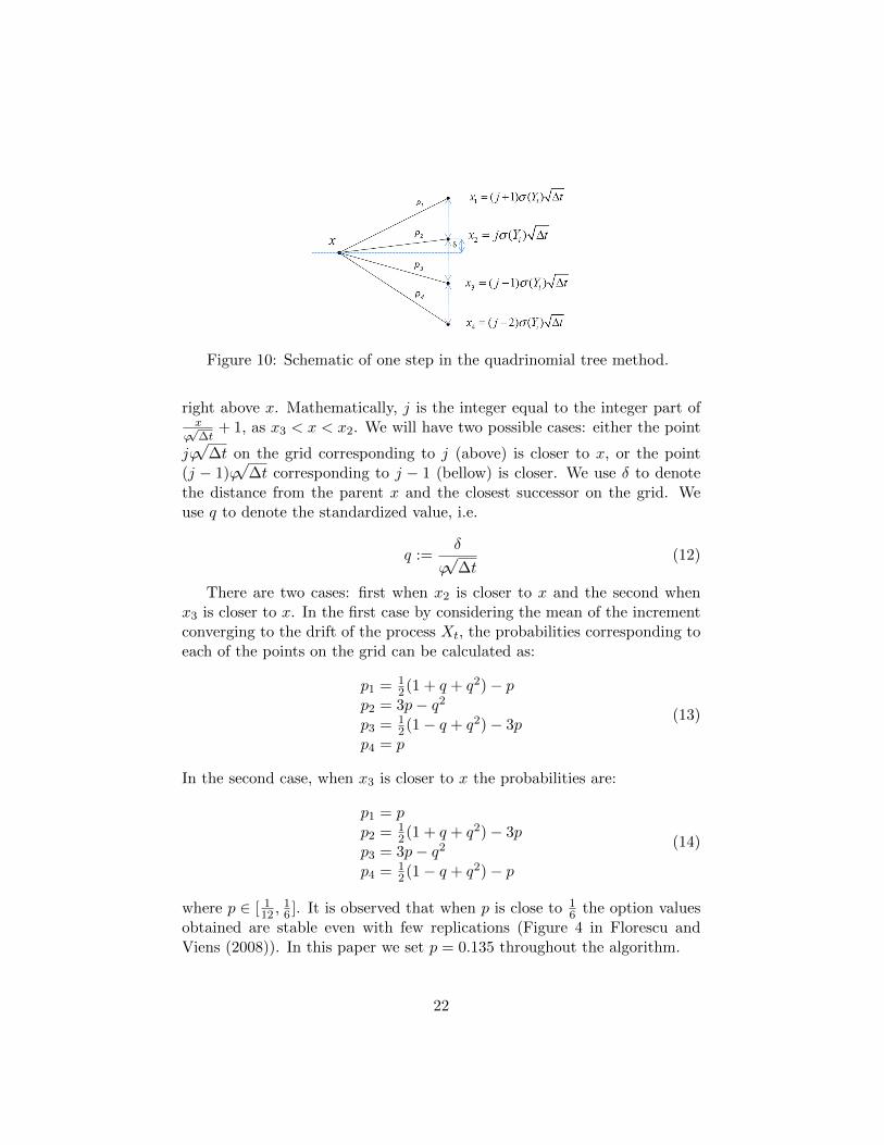
Figure 10: Schematic of one step in the quadrinomial tree method.

right above x. Mathematically, j is the integer equal to the integer part ofx

ϕ√

∆t+ 1, as x3 < x < x2. We will have two possible cases: either the point

jϕ√

∆t on the grid corresponding to j (above) is closer to x, or the point(j − 1)ϕ

√∆t corresponding to j − 1 (bellow) is closer. We use δ to denote

the distance from the parent x and the closest successor on the grid. Weuse q to denote the standardized value, i.e.

q :=δ

ϕ√

∆t(12)

There are two cases: first when x2 is closer to x and the second whenx3 is closer to x. In the first case by considering the mean of the incrementconverging to the drift of the process Xt, the probabilities corresponding toeach of the points on the grid can be calculated as:

p1 = 12(1 + q + q2)− p

p2 = 3p− q2

p3 = 12(1− q + q2)− 3p

p4 = p

(13)

In the second case, when x3 is closer to x the probabilities are:

p1 = pp2 = 1

2(1 + q + q2)− 3pp3 = 3p− q2

p4 = 12(1− q + q2)− p

(14)

where p ∈ [ 112 ,

16 ]. It is observed that when p is close to 1

6 the option valuesobtained are stable even with few replications (Figure 4 in Florescu andViens (2008)). In this paper we set p = 0.135 throughout the algorithm.

22

Step-by-Step Explanation of the Construction of VIX UsingStochastic Volatility Quadrinomial Tree Method

Here we use quadrinomial tree model to compute the price of a syntheticoptions with exact 30 days maturity using distribution of implied volatilityobtained from S&P500 as input. Then by Black and Scholes (1973) formula,we obtain the implied volatility of this synthetic option. We want to studywhether or not this implied volatility multiplied with 100 can better reflectthe market volatility.

There are four steps in the construction of this volatility index:

• Compute the implied volatilities of entire option chain on SP500 andconstruct an estimate for the distribution of current market volatility.The implied volatility is calculated by applying Black-Scholes formula.

• Use this estimated distribution as input to the quadrinomial tree method.Obtain the price of an at-the-money synthetic option with exactly 30day maturity.

• Compute the implied volatility of the synthetic option based on Black-Scholes formula once the 30-day synthetic option is priced.

• Obtain the estimated volatility index by multiplying the implied volatil-ity of the synthetic option by 100.

Please note that the most important step in the estimation is the choice ofproxy for the current stochastic volatility distribution.

References

Black, F. and M. Scholes (1973). The valuation of options and corporateliability. Journal of Political Economy 81, 637–654.

Bollen, N. and R. Whaley (2004, Apr.). Does net buying pressure affect theshape of implied volatility functions? Journal of Finance 59 (2), 711–753.

CBOE (2003). The new cboe volatility index-vix. white papers, CBOE.

Demeterfi, K., E. Derman, M. Kamal, and J. Zou (1999, March). Morethan you ever wanted to know about volatility swaps. Technical report,Goldman Sachs Quantitative Strategies Research Notes.

23

Florescu, I. and F. Viens (2008). Stochastic volatility: option pricing using amultinomial recombining tree. Applied Mathematical Finance Journal 15,151–181.

Jiang, G. J. and Y. S. Tian (2007). Extracting model-free volatility fromoption prices: An examination of the VIX index. Journal of Deriva-tives 14 (3), 35–60.

24