Construction of near optimal meshes for 3D curved domains ...

ORIGINAL ARTICLE

Construction of near optimal meshes for 3D curved domainswith thin sections and singularities for p-version method

Xiao-Juan Luo • Mark S. Shephard • Lu-Zhong Yin •

Robert M. O’Bara • Rocco Nastasi • Mark W. Beall

Received: 23 November 2005 / Accepted: 11 May 2007

Springer-Verlag London Limited 2010

Abstract The adaptive variable p- and hp-version finite

element method can achieve exponential convergence rate

when a near optimal finite element mesh is provided. For

general 3D domains, near optimal p-version meshes require

large curved elements over the smooth portions of the

domain, geometrically graded curved elements to the sin-

gular edges and vertices, and a controlled layer of curved

prismatic elements in the thin sections. This paper presents

a procedure that accepts a CAD solid model as input and

creates a curved mesh with the desired characteristics. One

key component of the procedure is the automatic identifi-

cation of thin sections of the model through a set of discrete

medial surface points computed from an Octree-based

tracing algorithm and the generation of prismatic elements

in the thin directions in those sections. The second key

component is the identification of geometric singular edges

and the generation of geometrically graded meshes in the

appropriate directions from the edges. Curved local mesh

modification operations are applied to ensure the mesh can

be curved to the geometry to the required level of geo-

metric approximation.

Keywords Mesh generation Variable p-version

method Thin geometric section

1 Introduction

To achieve the exponential convergence rate of the

p-version finite element method, a proper mesh that

accounts for the characteristic of the exact solution, which

is determined by the shape of the domain, the boundary

conditions, the loading functions, and the material param-

eters, etc., is needed. In the case of a piecewise smooth

domain so that the solution is smooth, the p-version mesh

requires the level of geometric approximation of those

finite element faces and edges that lie on curved domain

boundaries increases when the order of the finite element

basis functions is increased. Otherwise, the error due to

geometric approximation will become the dominant error,

thus, yielding any further increase in finite element order

meaningless [1, 2]. The satisfaction of geometric approxi-

mation needs for the p-version meshes is met through the

assignment of appropriate geometric shapes to mesh edges

and faces classified on the curved model boundaries. In the

neighborhood of a model edge whose interior dihedral

angle is larger than p, the exact solution is smooth along

the direction of the model edge and singular in the per-

pendicular directions. Effective resolution of the singular-

ities requires the mesh to be geometrically graded in those

directions [3, 4].

Thin sections of the domain are defined as portions in

which one dimension is small with respect to the other two.

Thin sections are often modeled by applying dimensional

X.-J. Luo M. S. Shephard (&) L.-Z. Yin

Scientific Computation Research Center,

Rensselaer Polytechnic Institute,

Troy, NY 12180, USA

e-mail: [email protected]

X.-J. Luo


R. M. O’Bara

Kitware Inc., Clifton Park, NY 12065, USA

R. Nastasi M. W. Beall

Simmetrix Inc., Clifton Park, NY 12065, USA


M. W. Beall


123

Engineering with Computers

DOI 10.1007/s00366-009-0163-0

reduction methods to use 2D shell elements [5, 6]. How-

ever, the application of such methods requires handling the

interconnection between the dimensional reduced elements

to fully 3D solid elements in non-thin sections which is

difficult [7]. An alternative is to model the whole domain

by 3D elements allowing low order deformation modes in

the thickness direction based on the p-version hierarchic

plate models developed by Szabo et al. [8] during 1980s.

Tetrahedral meshes created by current automatic mesh

generators do not effectively model the low order thickness

deformation modes due to the presence of diagonals across

the thickness of the thin direction as shown in Fig. 1. The

most effective p-version solutions are obtained if the mesh

employs prismatic elements such that through the thickness

diagonals are avoided in thin or other critical sections of

the domain.

In this paper, we present a procedure that considers the

singular edges and thin sections in the process of gener-

ating curved meshes for use in the p-version finite element

method. Starting from a CAD model and a coarse surface

mesh that can be obtained from mesh generators developed

for h-version finite element method [9], a set of discrete

medial surface points is computed through an Octree-based

tracing algorithm. These points, along with mesh topo-

logical adjacency and classification against the geometric

model, are used to automatically identify the thin sections

within the domain. The surface mesh triangulation of those

thin sections is then modified in a way that pairs of trian-

gles on the opposite thin geometric sections can be directly

connected to create prismatic elements without through the

thickness diagonals. The singular model edges are isolated

at the model level using CAD model geometric information

such as face normal vectors at a defined point on the model

boundary to compute the interior dihedral angles of the

model edges. Surface mesh modification is needed in the

neighborhood of the isolated singular model edges to

produce enough space to construct geometrically graded

elements in a cylindrical region around those edges. After

dealing with the thin sections and singular model edges, the

remaining portions of the domain are filled by a volume

mesh generator with tetrahedral elements. An enhanced

mesh curving procedure [10] is applied to curve the mesh

entities by:

– Curving the mesh for thin sections and singular model

edges before curving any other mesh entities to ensure

a proper structure is maintained in the curved mesh.

– Curving the remaining mesh entities classified on curved

boundaries to sufficient level of geometric approxima-

tion. Since curving entities can lead to invalid elements,

this step includes the application of curved mesh

modification operations including entity shape change,

splits, collapses and swaps as needed to ensure that a

valid mesh with acceptable curved elements is created.

The paper is organized as follows: Sect. 2 presents the

procedure to automatically identify and mesh thin sections.

Section 3 discusses the isolation and meshing of the sin-

gular model edges. Section 4 describes the volume mesh

generation for the remaining domains. Section 5 presents a

mesh curving procedure to effectively curve a straight-

sided mesh in a controlled manner to maintain the mesh

structure for the p-version finite element method. Curved

mesh examples are given in Sect. 6.

2 Identifying and meshing thin sections

The geometric characteristic indicating a thin geometric

section is the dimension through the thickness being sub-

stantially less than the ‘‘in-surface’’ dimensions as mea-

sured by the desired element size. In this section, we present

a procedure to automatically identify and mesh thin sections

starting from a surface triangulation of the model that has

been sized to have triangles of the size desired in the final

curved mesh in non-critical areas. The starting surface mesh

is generated using the mesh generators developed for the

h-version finite element method [9] that is classified against

the CAD geometric model to define the relationship

between the mesh and the geometric domain [11].

2.1 Nomenclature

The nomenclature used to describe the mesh topology and

the classification of the mesh to the geometric model are

given as follows:

V the model, V [ G, M, O where G signifies

the geometric model, O signifies the Octree

model, and M signifies the mesh model.

VVd a set of topological entities of dimension d in

model V.Fig. 1 Tetrahedral mesh with diagonals across the thickness of the

thin sections


123

Vdi the ith entity of dimension d in model V. d = 0

for a vertex, d = 1 for an edge, d = 2 for a

face, and d = 3 for a region.

Vdi closure of the topological entity Vd

i :

Mdii G

dj

j classification indicating the unique association

of entity Mdii with entity G

dj

j ; di dj:

Gdj a set of mesh entities on thin sections uniquely

classified on model entity Gdj :

E0 a set of discrete points on the medial surface of

model G.

VoriðGdi Þ the Voronoi region associated with geometric

model entity Gdi :

2.2 Octree-based tracing algorithm to compute

the discrete medial surface points

A point on the medial surface can provide the local

thickness as the distance measured by a pair of closest

boundary points on ‘‘opposite’’ boundary entities. This

distance is compared to the triangle edge length and the

section is determined to be thin at that location if the ratio

of the thickness to the edge length is below a prescribed

value.

Based on the property that a closed geometrical model

has a closed set of medial surfaces [12], the medial surface

points are computed through an Octree-based tracing

algorithm that starts from a surface mesh triangulation of

the geometric model and outputs a set of discrete points on

the medial surfaces. The tracing algorithm contains the

following steps:

– Construct Octree model based on the surface

triangulation.

– Determine octants with edges intersecting the medial

surfaces.

– Resolve the intersections between the octant edges and

the medial surfaces to determine the medial surface

points.

The algorithm is terminated after finding and processing

all the intersecting octant edges. The classification infor-

mation of the surface triangulation is used to skip the

unnecessary calculations of the closest points related to

pair of triangles classified on the same C1 continuous

model face.

2.2.1 Constructing Octree model based on the surface

triangulation

The Octree model is constructed by inserting the surface

mesh entities into boundary octants of the same order to

ensure that the computed medial surface points are dense

enough to isolate thin sections. The size of the interior

octants is controlled by recursive subdivision such that the

neighbor medial octants are different by not more than one

level.

2.2.2 Determining medial octants

A medial octant is defined as an octant whose octant edges

intersect the medial surface. The second step in the tracing

algorithm is to determine the medial octants from the

Octree model that employs the relationship between the

Voronoi regions and medial surfaces of a geometric model

[13, 14]. It is indicated in Ref. [13] that the medial surfaces

are identical to the boundaries of the Voronoi regions for a

convex model. In the case of a non-convex model, the

boundaries of the Voronoi regions are a superset of

the medial surfaces that do not include the boundaries of

the Voronoi regions associated with the re-entrant model

edges. Figure 2a shows the Voronoi regions and the medial

surfaces for a convex model. Figure 2b shows the Voronoi

regions and the medial surfaces for a non-convex model

that indicates the medial surfaces do not include two of the

boundaries of the Voronoi region VorifG00g:

G10Vori( )

G13 G1

1G13

G12

G11

G10

G12

Vori( )

Vori( )

Vori( )

Medial surface

(a)

G10

G10Vori( )

G11Vori( ) G1

1

G12

G13G1

3Vori( )

G12Vori( )

G00

G14

G14

G00

G15 G1

5 )Vori(

)Vori(

Vori( )

Medial surfaceBoundaries not medial surface

(b)

Fig. 2 2D examples to demonstrate the relationship between Voronoi

regions and medial surfaces: a convex model and b non-convex

model


123

Based on the relationship between the Voronoi regions

and the medial surfaces, an octant edge O1i that is not

adjacent to one re-entrant edge or corner intersects the

medial surface when its bounding octant vertices are in

different Voronoi regions. To determine the correct

Voronoi region an octant vertex O0i is in, the closest points

of the octant vertex O0i to the model boundaries are used. In

the case where the octant vertex O0i only has one closest

point on model entity Gdi ;O

0i is interior to the Voronoi

region of Gdi : If multiple closest points exist, the octant

vertex is on the medial surface. Therefore, the medial

octants can be determined as those whose octant edges

intersect the medial surfaces. Figure 2 also shows the

completed medial octants for both the convex and non-

convex models.

2.2.3 Resolving intersections to determine medial

surface points

One or more octant edges of the medial octants can have

one or multiple intersections with the medial surfaces that

need to be resolved to determine the medial surface points.

After traversing the medial octants and placing the octant

edges in the list, the algorithm processes each octant edge

individually as follows.

Assume that an octant edge has one intersection medial

point, for example, the octant edge bounded by octant

vertices O02;O

03 in Fig. 3. The medial point can be found

through the linear interpolation of the octant edge as

E01 ¼ ð1 tÞ O0

2 þ t O03 ð1Þ

due to the equidistant condition to the boundary entities

whose associated Voronoi regions, the bounded octant

vertices O02;O

03; are in [13], where the bold letters denote

the coordinate vectors. The t used to compute the

coordinates of the intersection point is given as

t ¼ ðO03 O0

2Þ n3 þ d3 d2

ðO02 O0

3Þ n2 þ ðO03 O0

2Þ n3

; ð2Þ

where d2 and d3 are the distances from the octant vertices

to the closest model face, and n2 and n3 are the unit vectors

from O02;O

03 to their closest points on the boundaries as

shown in Fig. 3.

After obtaining the assumed medial surface point, the

distances from that point to its closest points on the

boundary are used to determine whether one or multiple

intersections exist between the octant edge and the medial

surface. The equal distances indicate one intersection as

E01 in Fig. 3. In the case where the distances are different

as E00 in Fig. 3, there are multiple intersection points.

Recursively subdividing the edge at the obtained location

is needed till one intersection is found on the processed

segment. For example, in Fig. 3, the procedure computes

the medial surface points between E00;O

00 and E0

0;O01

recursively.

This procedure terminates when all medial octant edges

have been processed and a set of discrete medial surface

points are obtained.

Figure 4 shows the calculation of medial surface points

as solid dots for a 3D curved domain using the tracing

algorithm.

2.3 Collecting the starting thin section triangle sets

Given a set of intersecting points between the medial sur-

faces and medial octants obtained from Sect. 2.2, a can-

didate thin section triangle pair can be determined. As an

example shown in Fig. 5, a pair of triangles, M2i and M2

i0 is

a candidate thin section triangle pair if there exists a pair

of closest boundary points P1 and P2 from a medial surface

point E0i ; such that P1 M

2

i and P2 M2

i0 ; and the ratio of

thickness (defined as the diameter of the maximum

inscribed sphere associated with E0i ) to the average edge

length of M2i and M2

i0 is smaller than a default value, for

example, 1/2 shown in Fig. 5.

Figure 6 shows an example of a 2D situation with a set

of medial surface points and the associated candidate pairs

thin section mesh edges ðM1j ;M

1j0 Þ: A candidate thin section

triangle pair is further processed to ensure that all points on

their closures meet the condition. As for the 2D example in

Fig. 6, the pair ðM10 ;M

100 Þ associated to the medial point E0

0

will be determined as a non-thin section pair because the

O20

O30

2n2d

3

3

E10

O10

E00

O00

Medial surface

t

1−t

DirectionDistance

DirectionDistance

nd

Fig. 3 A 2D example to demonstrate the calculation of the medial

surface points for medial octant edges


123

thickness associated with mesh vertices ðM00 ;M

000 Þ is not

small enough to meet the thin section condition.

The procedure to collect the initial thin section triangles

starts from traversing each discrete medial surface point

and its associated opposite pair of triangles. If the pair of

triangles is determined to be thin, the triangles are placed

into appropriate collecting triangle sets G2j uniquely

determined based on the geometric classification informa-

tion of the mesh faces. At this point, each G2j is uniquely

associated with a G2j : The identity tags of ‘‘opposite’’ sets

for G2j can be recorded during the construction of G2

j :

Generally, G2j may have one or more opposite sets denoted

as oppðG2j Þ: The simple 2D example in Fig. 6 shows that

G11 ¼ fM1

10 ;M120 ;M

130 g; oppðG1

1Þ ¼ fG12; G

13g; ð3Þ

G12 ¼ fM1

3 ;M14g; oppðG1

2Þ ¼ fG11g; ð4Þ

G13 ¼ fM1

1 ;M12g; oppðG1

3Þ ¼ fG11g: ð5Þ

The procedure is terminated when every discrete medial

surface point is processed.

2.4 Determining the missing thin section triangles

The majority of thin section triangles are identified using

the medial surface points. However, some are missed

because the closest points of the discrete medial surface

points are not in their closures. As an example, M13 in Fig. 6

will not be identified as thin section triangle because none

of the closest points of the medial surface points E00;E

01;E

02;

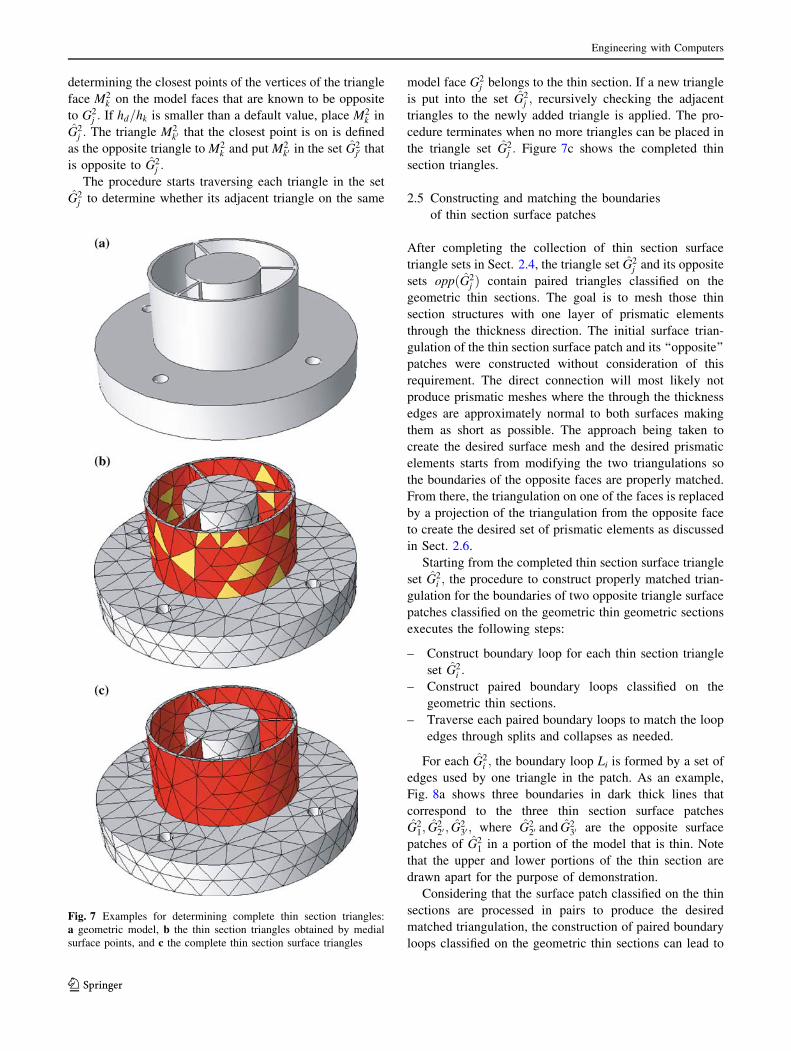
and E03 hit its closure. Figure 7b also shows the identified

thin section triangles marked as dark and the missing tri-

angles marked as light gray for a complex 3D geometry. To

determine whether a missing triangle M2k classified on G2

j

belongs to G2j ; the comparison between the local thickness

hd and the local mesh size hk at mesh face M2k is needed.

hk is computed as the longest edge length connected to

the vertices of the triangle face M2k : hd is obtained by

Fig. 4 The medial surface points for a 3D curved domain: a initial

surface triangulation, b medial surface points, and c close-up view of

the medial surface points on the top cylindrical portion

M2i’

M2i P 1

P 2

E 0i

Fig. 5 Definition of thin section triangle pair determined by a medial

surface point

G00G00

M01

G13

M11

M21M3

1M41

M0’1

M2’1M3’

1 M1’1

E00

E10

M0’0

M00

G12

G11

E20E3

0

Fig. 6 An example to demonstrate the collection of the starting

triangle sets


123

determining the closest points of the vertices of the triangle

face M2k on the model faces that are known to be opposite

to G2j : If hd=hk is smaller than a default value, place M2

k in

G2j : The triangle M2

k0 that the closest point is on is defined

as the opposite triangle to M2k and put M2

k0 in the set G2j0 that

is opposite to G2j :

The procedure starts traversing each triangle in the set

G2j to determine whether its adjacent triangle on the same

model face G2j belongs to the thin section. If a new triangle

is put into the set G2j ; recursively checking the adjacent

triangles to the newly added triangle is applied. The pro-

cedure terminates when no more triangles can be placed in

the triangle set G2j : Figure 7c shows the completed thin

section triangles.

2.5 Constructing and matching the boundaries

of thin section surface patches

After completing the collection of thin section surface

triangle sets in Sect. 2.4, the triangle set G2j and its opposite

sets oppðG2j Þ contain paired triangles classified on the

geometric thin sections. The goal is to mesh those thin

section structures with one layer of prismatic elements

through the thickness direction. The initial surface trian-

gulation of the thin section surface patch and its ‘‘opposite’’

patches were constructed without consideration of this

requirement. The direct connection will most likely not

produce prismatic meshes where the through the thickness

edges are approximately normal to both surfaces making

them as short as possible. The approach being taken to

create the desired surface mesh and the desired prismatic

elements starts from modifying the two triangulations so

the boundaries of the opposite faces are properly matched.

From there, the triangulation on one of the faces is replaced

by a projection of the triangulation from the opposite face

to create the desired set of prismatic elements as discussed

in Sect. 2.6.

Starting from the completed thin section surface triangle

set G2i ; the procedure to construct properly matched trian-

gulation for the boundaries of two opposite triangle surface

patches classified on the geometric thin geometric sections

executes the following steps:

– Construct boundary loop for each thin section triangle

set G2i :

– Construct paired boundary loops classified on the

geometric thin sections.

– Traverse each paired boundary loops to match the loop

edges through splits and collapses as needed.

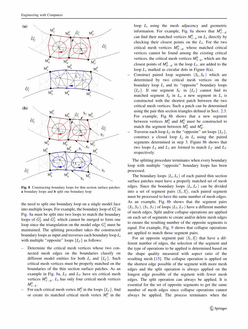
For each G2i ; the boundary loop Li is formed by a set of

edges used by one triangle in the patch. As an example,

Fig. 8a shows three boundaries in dark thick lines that

correspond to the three thin section surface patches

G21; G

220 ; G

230 ; where G2

20 and G230 are the opposite surface

patches of G21 in a portion of the model that is thin. Note

that the upper and lower portions of the thin section are

drawn apart for the purpose of demonstration.

Considering that the surface patch classified on the thin

sections are processed in pairs to produce the desired

matched triangulation, the construction of paired boundary

loops classified on the geometric thin sections can lead to

Fig. 7 Examples for determining complete thin section triangles:

a geometric model, b the thin section triangles obtained by medial

surface points, and c the complete thin section surface triangles


123

the need to split one boundary loop on a single model face

into multiple loops. For example, the boundary loop of G21 in

Fig. 8a must be split into two loops to match the boundary

loops of G220 and G2

30 which cannot be merged to form one

loop since the triangulation on the model edge G11 must be

maintained. The splitting procedure takes the constructed

boundary loops as input and traverses each boundary loop Li

with multiple ‘‘opposite’’ loops fLj0 g as follows:

– Determine the critical mesh vertices whose two con-

nected mesh edges on the boundaries classify on

different model entities for both Li and fLj0 g: Such

critical mesh vertices must be properly matched on the

boundaries of the thin section surface patches. As an

example in Fig. 8a, L20 and L30 have six critical mesh

vertices M01060 : L1 has only four critical mesh vertices

M014:

– For each critical mesh vertex M0i0 in the loops fLj0 g; find

or create its matched critical mesh vertex M0i in the

loop Li using the mesh adjacency and geometric

information. For example, Fig. 8a shows that M01040

can find their matched vertices M014 on L1 directly by

checking their closest points on the L1. For the two

critical mesh vertices M05060 whose matched critical

vertices cannot be found among the existing critical

vertices, the critical mesh vertices M056; which are the

closest points of M05060 in the loop L1, are added to the

loop L1 marked as circular dots in Figure 8(a).

– Construct paired loop segments ðSk; Sk0 Þ which are

determined by two critical mesh vertices on the

boundary loop Li and its ‘‘opposite’’ boundary loops

fLj0 g: If one segment Sk0 in fLj0 g cannot find its

matched segment Sk in Li, a new segment in Li is

constructed with the shortest patch between the two

critical mesh vertices. Such a patch can be determined

using the pair thin section triangles defined in Sect. 2.3.

For example, Fig. 8b shows that a new segment

between vertices M05 and M0

6 must be constructed to

match the segment between M050 and M0

60 :

– Traverse each loop Lj0 in the ‘‘opposite’’ set loops fLj0 g;construct a closed loop Lj in Li using the paired

segments determined in step 3. Figure 8b shows that

two loops L2 and L3 are formed to match L20 and L30

respectively.

The splitting procedure terminates when every boundary

loop with multiple ‘‘opposite’’ boundary loops has been

processed.

The boundary loops ðLi; Li0 Þ of each paired thin section

surface patches must have a properly matched set of mesh

edges. Since the boundary loops ðLi; Li0 Þ can be divided

into a set of segment pairs ðSi; S0iÞ; each paired segment

must be processed to have the same number of mesh edges.

As an example, Fig. 8b shows that the segment pairs

ðS2; S20 Þ; ðS3; S30 Þ of loops ðL3; L30 Þ have a different number

of mesh edges. Split and/or collapse operations are applied

on each set of segments to create and/or delete mesh edges

to ensure the resulting number of the opposite segments is

equal. For example, Fig. 9 shows that collapse operations

are applied to match those segment pairs.

For an opposite segment pair ðSi; S0iÞ that have a dif-

ferent number of edges, the selection of the segment and

the type of operations to be applied is determined based on

the shape quality measured with aspect ratio of the

resulting mesh [15]. The collapse operation is applied on

the shortest edge possible of the segment with more mesh

edges and the split operation is always applied on the

longest edge possible of the segment with fewer mesh

edges. The split operation can always be applied. It is

essential for the set of opposite segments to get the same

number of mesh edges since collapse operations cannot

always be applied. The process terminates when the

M04 M0

6 M03

M05

M01’ M0

2’

M04’ M0

6’ M03’

M01 M0

1

L 1

L 2’ L 3’

G22’

2G3’

G21

G11M0

5’

(a)

M04 M0

6 M03

M05

M01’ M0

2’

M04’ M0

6’ M03’

M01 M0

1

L 2’ L 3’

G22’

2G3’

G21

G11M0

5’

L 2 L 3

S3

S3’

S2

S2’

S1

S1’

(b)

Fig. 8 Constructing boundary loops for thin section surface patches:

a boundary loops and b split one boundary loop


123

number of the mesh edges of the set of opposite segments

is equal.

2.6 Matching thin section surface patches to create

prismatic elements

After the two thin section surface patches have appropri-

ately matched boundary mesh edges, the thin section sur-

face triangulation with the worst aspect ratio quality [15] is

selected to be replaced by the triangulation of the other

surface patch. The deletion of the surface patch will pro-

duce an empty polygon whose boundary vertices need to be

moved to their target positions computed as the closest

points of the remaining surface patch on this model face as

shown in Fig. 10a. Since the empty polygon is connected

to the portion of surface triangulations that are not in thin

sections, moving the boundary vertices of the empty

polygon on the model face can cause invalid elements on

the remaining surface triangulation as shown in Fig. 10.

For example, the mesh faces M22 and M2

3 become invalid

because of the movement of mesh vertex M00 : The invalid

elements are corrected by applying local mesh modifica-

tions [15]. As an example, collapsing vertex M03 to M0

0 can

eliminate the invalid mesh faces M22 and M2

3 shown in

Fig. 10b. The remaining thin section surface patches can

then be projected to their opposite model faces to create

topological and geometrical matched pair triangles and the

prismatic thin section elements are created by directly

connecting those matched pair triangles.

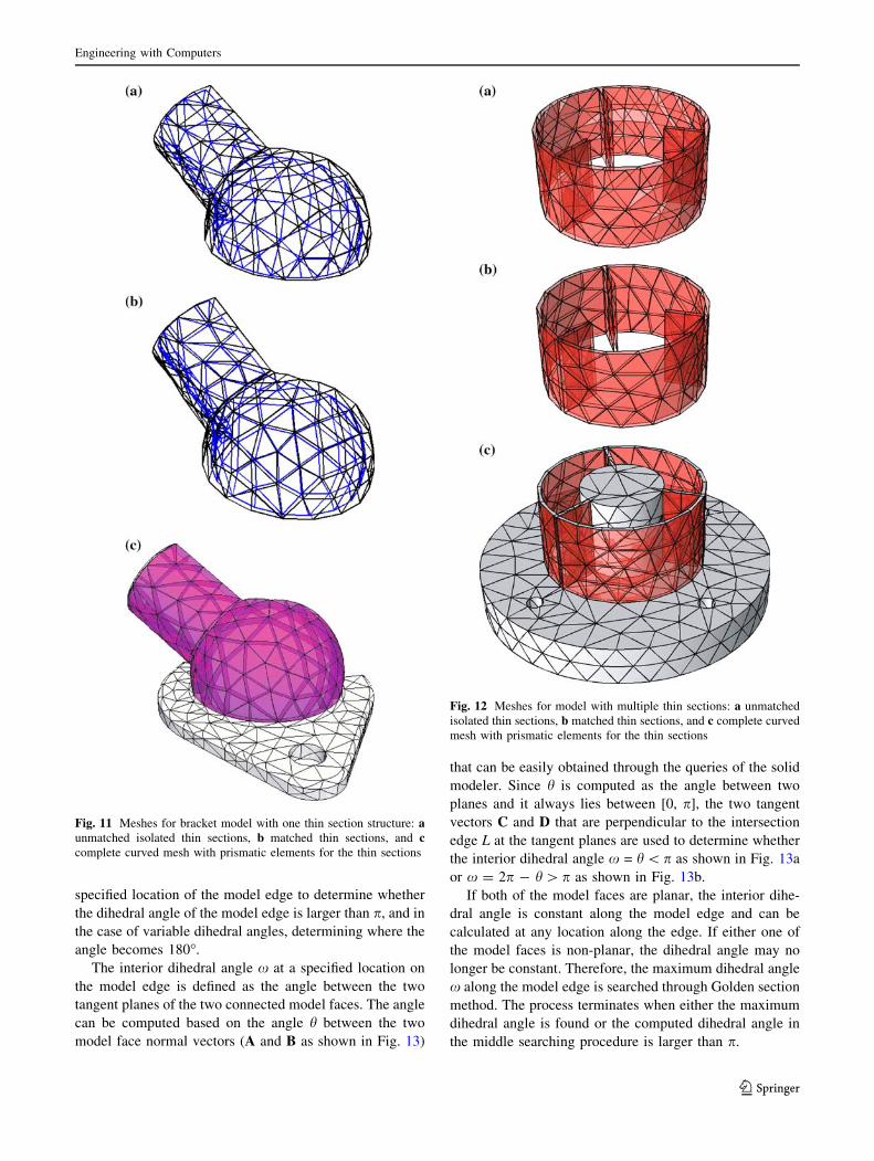
Figures 11 and 12 show two mesh results for 3D curved

geometric models with thin sections. Figures 11a and 12a

show the isolated opposite thin section surface patches that

are not yet matched and Figs. 11b and 12b show the mat-

ched thin sections. Figures 11c and 12c are complete

curved meshes with the thin section surface patches

matched and the prismatic thin section elements created.

The volume meshes are completed and the meshes are

properly curved to the domain boundary using the proce-

dures presented in Sects. 4 and 5, respectively.

3 Isolating and meshing singular model edges

After isolating and meshing the thin sections, the singular

edges are determined and appropriately meshed with geo-

metric graded meshes. The singular edges are isolated as

the set of model edges whose interior dihedral angles are

larger than p [3, 4],

G1i ¼ fG1

i j xi pg: ð6Þ

Since the interior dihedral angle xi for a model edge G1i in

a curved domain can vary, the variation x along the model

edge is checked using the interior dihedral angle x at a

M04 M0

6 M03

M05

M01’ M0

2’

M04’ M0

6’ M03’

M01 M0

1

L 2’ L 3’

G22’

2G3’

G21

G11M0

5’

L 2 L 3

S3

S3’

S2

S2’

S1

S1’

Fig. 9 Matching boundary loops for thin section surface patches

M04 M0

3

M01’ M0

2’

M04’ M0

3’

M01 M0

1

G22’

2G3’

G21

S2

S2’

M00

M22 M2

3

M03

Invalid elements ,

(a)

M04 M0

3

M01’ M0

2’

M04’ M0

3’

M01 M0

1

G22’

2G3’

G21

S2

S2’

(b)

Fig. 10 Matching the thin section surface patches: a deleting on

surface patch and move the boundaries and b copying the remaining

surface patch


123

specified location of the model edge to determine whether

the dihedral angle of the model edge is larger than p, and in

the case of variable dihedral angles, determining where the

angle becomes 180.

The interior dihedral angle x at a specified location on

the model edge is defined as the angle between the two

tangent planes of the two connected model faces. The angle

can be computed based on the angle h between the two

model face normal vectors (A and B as shown in Fig. 13)

that can be easily obtained through the queries of the solid

modeler. Since h is computed as the angle between two

planes and it always lies between [0, p], the two tangent

vectors C and D that are perpendicular to the intersection

edge L at the tangent planes are used to determine whether

the interior dihedral angle x = h\p as shown in Fig. 13a

or x = 2p - h[ p as shown in Fig. 13b.

If both of the model faces are planar, the interior dihe-

dral angle is constant along the model edge and can be

calculated at any location along the edge. If either one of

the model faces is non-planar, the dihedral angle may no

longer be constant. Therefore, the maximum dihedral angle

x along the model edge is searched through Golden section

method. The process terminates when either the maximum

dihedral angle is found or the computed dihedral angle in

the middle searching procedure is larger than p.

Fig. 11 Meshes for bracket model with one thin section structure: aunmatched isolated thin sections, b matched thin sections, and ccomplete curved mesh with prismatic elements for the thin sections

Fig. 12 Meshes for model with multiple thin sections: a unmatched

isolated thin sections, b matched thin sections, and c complete curved

mesh with prismatic elements for the thin sections


123

Starting from the linear surface triangulation, geomet-

rically graded meshes are generated around the isolated

singular edges using the growth curves originated from the

surface nodes [16]. The growth curves are constructed with

respect to the user-requested layer sizes. An interior growth

curve is a straight line whose nodes except the first are

classified in the model region. The nodes of a boundary

growth curve are classified on the model boundaries [16].

These nodes on the growth curves are connected to form

the cylindrical elements of the layer mesh. The intersection

between the exposed boundary layer mesh faces and sur-

face mesh faces is checked. If there are intersections, it is

necessary to reduce the height of a layer, or trim the

number of layers through the thickness in order to resolve

the intersections [16]. Each step in the process performs

checks to ensure the validity of the mesh and to optimize

the quality of the created mesh entities.

The character of the geometrically graded mesh gener-

ation is controlled through a set of attributes applied to the

model entities being isolated. The attributes include the

total height, gradation factor, and number of layers [10].

The total height of the graded mesh toward to a singular

model edge is automatically chosen by the procedure as

one half of the shortest distance from the model edge to

other non-connected model faces. A non-connected entity

is one which does not share any common lower order

model entities. The gradation factor is chosen as 0.15 to be

optimal for strong solution singularities [17]. Two initial

layers of elements are generated that usually will be reset

in the adaptive analysis.

Figure 14a shows a 3D curved geometric model and the

isolated singular model edges and the geometrical graded

meshes of linear elements around them are shown in

Fig. 14(b).

4 Volume mesh generation

After constructing the controlled volume mesh in the thin

sections and around the singular edges, the mesh for the 3D

domain contains a linear surface mesh and the prismatic

and hexahedral elements (see Sects. 2, 3). The remaining

domains that are a set of 3D polyhedron formed by the

surface mesh triangles and the boundary quadrilateral faces

of the prism and hexahedral elements are handed to a

generalized volume mesh generator [9]. The volume mesh

generator can create tetrahedral elements for complex

geometric domains so long as the boundary of that geom-

etry is triangulated. The requirement leads to the need of

splitting prism and hexahedral elements or adding pyra-

mids next to them to produce triangle faces. Adding

θ0

E0

G12

G22Ω

A

B

C

D

A+B

C+D

L(a)

E0

G12

G22

θ0

A

C

D

A+B

C+D

Ω

L

(b)

Fig. 13 Computation of the interior dihedral angle at points E0:

a x = h0 \p and b x = 2p - h0 [p

Fig. 14 Automatically isolate and mesh singular model edges:

a geometric model and b isolated singular edges with geometrically

graded mesh


123

pyramids is a better choice since it will not alter the con-

trolled meshes created in the critical regions.

An effective approach to add pyramid elements is to

connect the exposed quadrilateral faces to a vertex on the

surface mesh, one of whose connected triangles is topo-

logically adjacent to the prism or hexahedral elements. As

an example, Fig. 15 shows three candidate vertices for the

quadrilateral face M20 for a model with thin sections. The

criteria to select the appropriate vertex over the other

possible vertices depends on the shape quality of the pyr-

amid element to be created, for example, vertex M00 in

Fig. 15 is the select vertex. An alternative is to introduce a

new vertex interior to the domain out from the quadrilateral

faces to create a pyramid element.

There are situations where adding pyramid elements

may fail due to the unacceptable shape quality or no space

left for the new vertices. In this case, the process will split

one layer of prism or hexahedral elements by introducing

one interior vertex inside the original element. The

approach is a local operation that only affects the element

being split to create the needed triangle faces. As an

example, the prism region with quadrilateral face M21 in

Fig. 15 needs to be split. The template to split a prism or

hexahedral element into a combination of tetrahedra and

pyramids is a function of how many quadrilateral faces are

exposed. Figure 16 shows two templates to split one prism

element. Splitting one quadrilateral face of a prismatic

element produces four tetrahedral and two pyramid ele-

ments and splitting two quadrilateral faces produces six

tetrahedral and one pyramid element. The location of the

interior vertices was computed with centroid parameter

coordinate (1/3, 1/3, 0) on the original prismatic element.

The procedure to isolate the thin section does not allow one

single prismatic element over the isolated thin geometric

thin section. Therefore, the case of three exposed faces of a

prismatic element does not need to be considered.

5 Mesh curving

The volume mesh created at this point is a linear straight-

sided mesh with mixed topological mesh that contains

tetrahedral, prism, hexahedral, and pyramid elements. The

mesh entities classified on the curved boundaries must be

appropriately curved to sufficient geometric approximation

for the p-version finite element method. A Bezier approx-

imate geometry representation [18] is used to determine

appropriate shapes for the mesh entities on the curved

boundaries. This approach has two key advantages [10]:

– Computationally efficient algorithms for degree eleva-

tion and subdivision can extend the geometric approx-

imation up to any order.

– The convex hull property provides the effective shape

validity test for curved elements.

The conventional curving procedure [19, 20] does not

consider the mesh characteristics for the thin sections and

singular edges created in Sects. 2 and 3. In the process of

applying local mesh modifications to correct the invalid

elements caused by curving the mesh entities, these char-

acteristics are likely to be disrupted (see Fig. 20, top).

The enhanced mesh curving procedure presented in this

section curves the mesh entities in an appropriate order to

maintain the characters of the p-version meshes. The

application of the curved local mesh modification opera-

tions is the key technique to ensure that a valid curved

mesh is obtained [18].

5.1 Curve the prismatic thin section meshes

For the prismatic meshes classified on the curved thin

sections, the process curves the prismatic elements one at a

M20

M21

M00Selected vertex

Candidate vertices

New vertex inside prism element

close−up view

Fig. 15 Adding pyramid or splitting prism elements

Fig. 16 Templates to split prism elements (left) 4 tetrahedra and 2

pyramid (right) 6 tetrahedra and 1 pyramid


123

time to maintain the structure as demonstrated with an

example in Fig. 17. Figure 17a shows one of the quadri-

lateral faces of a prismatic region. Figure 17b shows that

the quadrilateral face becomes invalid after the mesh edge

M10 is curved to the boundary. The invalidity is caused by

the interference between the curved mesh edge M10 and the

uncurved mesh edge M11 : The conventional curving pro-

cedure [19] will apply local mesh modification operations

to eliminate the invalidity and the resulting mesh is shown

in Fig. 17c that disrupts the structures for the thin sections.

However, this invalidity is avoided if the mesh edges

M10 ;M

11 are curved to the boundary at the same time as

shown in Fig. 17d. Therefore, the process picks up one

prismatic element from the thin section meshes and curves

all the lower bounded mesh entities of the prismatic ele-

ment before applying the validity check. In the case that the

curved prismatic element remains invalid, curved local

mesh modification operations as discussed in Sect. 5.3 will

be applied to correct the invalidity.

5.2 Curve the graded meshes for singular model edges

To ensure a properly curved graded mesh around the sin-

gular features, the process simultaneously curves the mesh

entities on the boundary and those within the structured

layer above it. Figure 18 demonstrates this process with

Fig. 18a showing the linear structured layer mesh associ-

ated with a portion of a curved model edge. Figure 18b

shows how the local gradation would be disrupted if only

the mesh edge, M10 ; classified on the model edge G1

0 was

curved. To avoid this problem, the ‘‘parallel’’ and ‘‘diag-

onal’’ mesh edges (see Fig. 18a) are also curved such that

the entire layer maintains its gradation, and element shapes

are smooth. This process is accomplished by moving the

control points of the parallel and diagonal edges based on

how far the control points of the edge on the model

boundary are moved with consideration given to the

change in length of the edges being curved. The need to

account for the length of the edges being curved is dem-

onstrated in Fig. 18c, where all control points were moved

the same distance as the associated control points on the

mesh edge M10 classified on the curved boundary. It is clear

that the short edges are curved more than desired. The

method used scales the shape change of the base mesh edge

accounting for edge lengths as follows. Let Lbase; LPiand

LDibe the straight-sided edge length of the mesh edge on

the curved boundary (the base edge), ith parallel and ith

diagonal edge. The scale factors SPiand SDi

for ith parallel

and diagonal edges applied to their movements with

respect to that of the base edge are

SPi¼ LPi

Lbase

; ð7Þ

SDi¼ 0:5ðSPi1

þ SPiÞ: ð8Þ

Figure 18d shows a smooth curved isolation mesh using

this method. The curving procedure at this point only

curves the graded layer meshes as needed.

M10

M11

G10

G11

(a)

M10

M11

G10

G11

(b)

M10

G10

G11

M11 M1

1(c)

M10

G10

G11

M11(d)

Fig. 17 Curve the prismatic thin section meshes: a linear prismatic

elements and b curve M10 to G1

1 and cause invalidity, c local mesh

modification to correct the invalidity, and d simultaneously curve the

edges M10 ;M

11

G10

M10

Diagonal

Parallel

(a)

G10

M10

(b)

G10

M10

(c)

G10

M10

(d)

Fig. 18 Scaled curve graded mesh: a linear graded mesh, b curve M10

to G10; c curve the graded mesh the same as M1

0 ; and d scaled curve

craded mesh


123

5.3 Curve mesh entities on the curved boundaries

After curving the graded mesh around the isolated mesh

edges and the prismatic meshes for the thin sections, the

general curving procedure given in Ref. [10] curves the

remaining mesh edges/faces classified on curved model

boundaries. The entities are put into a list with the

attachment of a proposed Bezier geometric shape to curve

them to the boundary.

The process of curving the mesh entities traverses the

list. If the movement associated with this curving maintains

validity of the connected mesh entities, the entity is curved

and removed from the list. If any invalid entities arise,

additional processing is required. Since changing the shape

of a mesh entity changes the shape of the mesh entities it

bounds, the process of checking the validity of the mesh

must check the shape validity of the connected mesh

entities as well. This means that in addition to verifying no

self-intersection of the curved mesh face or edge, the shape

validity of the connected high-dimensional mesh entities

are checked. The verification of self-intersection of any

curved Bezier mesh edge or faces uses the variation

diminishing property that no straight line intersects a curve

more times than it intersects the curve’s control polygon

[21].

In cases when a mesh entity does cause an invalidity,

curved local mesh modification operations are applied [10].

After the needed mesh modifications are performed the

current mesh entity is removed from the list and any newly

created mesh entities classified on curved boundaries are

added to the list. The process ends when the list is empty.

6 Examples

Figure 19 shows the meshes without/with considering

gradation in the process of curving the mesh entities

around singular model edges.This example does not

contain thin sections. The bottom curved mesh in Fig. 19

is generated by considering the controlled meshes for the

singular edges, and the graded meshes around the curved

singular edges are maintained by comparing the top

curved mesh without considering the control of the mesh

gradation. Figure 20 is the close-up view of the graded

meshes around the curved singular model edges gener-

ated using the two different procedures. Table 1 presents

the statistics of the mesh entities of these two meshes. In

addition to maintaining the mesh gradation for the sin-

gular edges, the curving procedure considering gradation

uses 15% less elements because of the application of

prism and hexahedral over the tetrahedral elements

toward the singular model edges and the less require-

ments of the local refinement modification to correct the

invalid elements during mesh curving as shown in

Fig. 17.

Figure 21 shows an example with singular edges and

thin sections together. Three different meshes are shown:

curved isotropic volume mesh (type a), curved tetrahedral

mesh without considering thin sections and gradation

control (type b), and curved mixed mesh considering

curved entity gradation control and thin sections (type c).

The number of elements for the three cases is given in

Table 2. The statistics show that the curved mixed mesh

generated by applying the automatic p-version mesh pro-

cedure produces 1/2 the elements of the type b mesh which

does not account for the thin section or gradation control.

Figure 20 shows the close-up view of mesh around the

singular edge for type b and type c meshes. The gradation

for the type c mesh is maintained through the curving

procedure with gradation control.

Figure 22 shows a final 3D curved model with singular

edges and thin sections together. In this example, the thin

section represents a small portion of the domain. The sta-

tistics are shown in Table 3 that indicate the type c mesh

Fig. 19 Curved meshes for model with singularities: a curving

without considering gradation and b curving considering gradation


123

has 240 fewer elements, which is a 24% reduction in the

number of elements than the type b mesh.

7 Conclusion

This paper has discussed a procedure to automatically

generate near optimal meshes for general 3D curved

Fig. 20 Close-up view of curved meshes for models with singular-

model edges: a curving without considering gradation and b curving

considering gradation

Table 1 Statistics for curving model with singular edges without/

with considering gradation

Mesh a Mesh b

Regions 1,923 1,643

Faces 3,456 3,356

Edges 3,356 2,980

Vertices 467 406

Fig. 21 Examples meshes for model with singular edges and thin

sections: a type a: isotropic curved volume mesh, b type b: curved

mesh without considering gradation and thin sections, and c type c:

curved mixed mesh considering gradation and thin sections

Table 2 Statistics for curved models with singular edges and thin

sections in Fig. 21

Meshes Regions Gradation

Type a 306 0.0

Type b 705 0.15

Type c 350 0.15


123

domains with thin sections and singular model edges

suitable for adaptive variable p-version finite element

analysis. The procedure starts with the automatic isolation

of thin sections through a set of discrete medial surface

points computed from an Octree-based tracing algorithm.

Prismatic elements in the thin sections are generated

without long diagonals through the thickness directions.

The singular edges are isolated at the model level and

geometric graded elements are generated around those

singular edges. The linear meshes are curved in a proper

order. The controlled meshes for the critical regions are

curved before curving the mesh entities on the remainder of

the curved boundaries.

As the results demonstrate, the procedure has the

capability to produce suitable meshes for adaptive variable

p-version finite element analysis. The curved meshes sat-

isfy the optimal mesh requirements for 3D curved models

with thin sections and singular edges.

Acknowledgments This work was supported by the National Sci-

ence Foundation through SBIR grant number DMI-0132742.

References

1. Luo XJ, Shephard MS, Remacle JF, O’Bara RM, Beall MW,

Szabo BA, Actis R (2002) p-version mesh generation issues. In:

Proceedings of the 11th international meshing roundtable, Ithaca,

September, pp 343–354

2. Dey S, Shephard MS, Flaherty JE (1997) Geometry-based issues

associated with p-version finite element computations. Comput

Methods Appl Mech Engrg 150:39–55

3. Dorr MR (1984) The approximation of solutions of the elliptic

boundary-value problems via the p-version of the finite element

method. SIAM J Numer Anal 21(6):58–76

4. Babuska I, Suri M (1994) The p and h-p versions of the finite

element method, basic principles and properties. SIAM Rev

36(4):578–632

5. Reddy JN (1999) Theory and analysis of elastic plates. Taylor &

Francies, Philadelphia

6. Donaghy RJ, Armstrong CG, Price MA (2000) Dimensional

reduction of surface models for analysis. Eng Comput 16:24–35

7. Actis RL, Engelstad SP, Szabo BA (2002) Computational

requirements in design and design certification. In: Collection of

technical papers—43rd AIAA/ASME/ASCE/AHS/ASC struc-

tures. Structural dynamics and materials conference, Denver,

April, pp 1379–1389

8. Szabo BA, Sahrmann GJ (1988) Hierarchic plate and shell

models based on p-extension. Int J Numer Meth Eng 26:1855–

1881

9. Shephard MS, George MK (1992) Reliability of automatic 3D

mesh generation. Comput Methods Appl Mech Eng 101:443–462

10. Luo XJ, Shephard MS, Obara RM, Nastasia R, Beall MW (2004)

Automatic p-version mesh generation for curved domains. Eng

Comput 20:265–285

11. Beall MW, Shephard MS (1997) A general topology-based mesh

data structure. Int J Numer Meth Eng 40(9):1573–1596

12. Lieutier A (2004) Any open bounded subset of rn has the same

homotopy type as its medial axis. Comput Aided Des 36:1029–

1046

13. Patrikalakis NM, Gursoy HN (1990) Shape interrogation by

medial axis transform. In: ASME advances in design automation,

16th design automation conference, vol 23, Chicago, pp 77–88

14. Etzion M, Rappoport A (2002) Computing Voronoi skeletons of a

3-D polyhedron by space subdivision. Comput Geom 21:87–120

15. Li XR, Shephard MS, Beall MW (2003) Accounting for curved

domains in mesh adaptation. Int J Numer Meth Eng 150:247–276

16. Garimella R, Shephard MS (2000) Boundary layer mesh gener-

ation for viscous flow simulations in complex geometric domain.

Int J Numer Meth Eng 49(1–2):193–218

17. Szabo BA (1986) Mesh design for the p-version of the finite

element method. Comput Methods Appl Mech Eng 55:181–197

18. Luo XJ (2005) An automatic adaptive directional variable p-

version method in 3-D curved domains, Ph.D thesis. Rensselaer

Polytechnic Institute

19. Dey S, O’Bara RM, Shephard MS (2001) Curvilinear mesh

generation in 3D. Comput Aided Des 33:199–209

20. Sherwin SJ, Peiro J (2002) Mesh generation in curvilinear

domains using high order elements. Int J Numer Meth Eng

53:207–223

21. Farin G (1992) Curved and surfaces for computer aided geo-

metric design. Academic Press, New York

Fig. 22 Examples of meshes for models with singular edges and thin

sections: a isotropic curved volume mesh, b curved mesh without

considering gradation and thin sections, and c curved mixed mesh

considering gradation and thin sections

Table 3 Statistics for curved models with singular edges and thin

sections in Fig. 22

Meshes Regions Gradation

Type a 260 0.0

Type b 996 0.15

Type c 756 0.15


123

Construction of near optimal meshes for 3D curved domains ...

Documents

Transcript of Construction of near optimal meshes for 3D curved domains ...