CONSTRUCTION OF INELASTIC RESPONSE SPECTRA FOR

. SINGLE-DEGREE-OF-FREEDOM SYSTEMS

COMPUTER PROGRAM AND APPLICATIONS

By S.A. Mahin and J. Lin

A report on research sponsored by the

National Science Foundation

Report No. UCB/EERC-83/17

Earthquake Engineering Research Center

College of Engineering

University of California

Berkeley, California

June, 1983

50272-101 REPORT DOCUMENTATION 11. REPORT NO.

PAGE NSF/CEE-83030 I~ 3. Recipient's Accession No.

PBG I 2 0 B 8 311 4. Title and Subtitle 5. Report Date

CONSTRUCTION OF INELASTIC RESPONSE SPECTRA FOR SINGLE-DEGREE­OF-FREEDOM SYSTEMS: Computer Program and Applications

June 1983

7. Author(s)

S.A. Mahin and J. Lin 9. Performing Ol1i:anization Name and Address

Earthquake Engineering Research Center University of California 1301 South 46th Street Richmond, CA 94804

12. Sponsoring Organization Name and Add~s

National Science Foundation 1800 "G" Street NW Washington, DC 20550

15. Supplementary Notes

16. Abstract (limit: 200 words)

a. Performing O,.anlzation Rept. No.

UCB/EERC-83/17 10. ProJect/Ta.klWorlc Unit No.

11. Contract(C) or Gra.rt(G) No.

(C)

(G) CEE-8208079 13. Type of Report & Period Covered

14.

This report describes a computer program written to analyze the inelastic response of viscously damped single-degree-of-freedom systems to either support excitation or exter­nal loadings. Various methods of developing design aids based on computed inelastic response are discussed. The computer program nas been written to allow the user to con­veniently obtain detailed information regarding tne inelastic response of a system and to study systematically the effect of variations in the mechanical and dynamic characteristics of the system and of different excitations.

Theoretical formulations and solution scliemes used in the computer program are described. The definitions and limitations of different response indicies, including various types of ductility factors, are examined, Procedures for constructing ductility­based response spectra appropriate for design are presented. Several examples of using the computer program for generating response of single-degree-of-freedom systems and response spectra are presented for i 11 ustrati.on. Ooservati ons regarding ine 1 ast i c behavior of structures are also described, Conclusions regarding the applicability of these results and the need to extend these methods to mult;ple-degree.of-freedom systems are offered.

17. Document Analysis a. Descriptors

b. Identifiers/Open·Ended Terms

c. COSATI Field/Group

18. Availability Statemen~

Release Unlimited

(See _ANSI-Z39.18)

19. Security elns (This Report)

20. Security Cia .. (This Pap)

21. No. of Pages

S'-' 22. Price

OPT!ONAL FORM 272 (4=77) (Formerly NTIS-3S) Department of Commerce

- i -b

ABSTRACT

This report describes a computer program written to analyze the inelastic response of

viscously damped single-degree-of-freedom systems to either support excitation or external

loadings. Various methods of developing design aids based on computed inelastic response are

discussed. The computer program has been written to allow the user to conveniently obtain

detailed information regarding the inelastic response of a system and to study systematically the

effect of variations in the mechanical and dynamic characteristics of the system and of different

excitations.

Theoretical formulations and solution schemes used in the computer program are

described. The definitions and limitations of different response indicies, including various types

of ductility factors, are examined. Procedures for constructing ductility-based response spectra

appropriate for design are presented. Several examples of using the computer program for gen­

erating response of single-degree-of-freedom systems and response spectra are presented for

illustration. Observations regarding inelastic behavior of structures are also described. Conclu­

sions regarding the applicability of these results and the need to extend these methods to

multiple-degree-of-freedom systems are offered.

- ii -

ACKNOWLEDGEMENTS

The research presented in this report has been sponsored by the National Science Founda­

tion. The support is gratefully acknowledged. Opinions, findings, and conclusions or recom­

mendations expressed in this publication are those of the authors and do not necessarily reflect

the views of the National Science Foundation or the Earthquake Engineering Research Center,

University of California, Berkeley.

Credits are given to Mr. R. Herrera who was involved in the early development of the

computer program and to Mr. R. Klingner who developed the variable time step algorithm used

in the computer program. The drafting was prepared by Ms. G. Feazell. The contributions of

these persons to the publication of this report are appreciated.

- iii -

Table of Contents

ABSTRACT .......................................................................................................................... . i

ACKNOWLEDGEMENTS ................................................................................................... ii

TABLE OF CONTENTS .. ............ ................ ......... ............................... ................ ................. iii

1 INTRODUCTION ............................................................................................................. 1

1.1 Introductory Remarks .......... ........................ .................................. .......... .................. 1

1.2 Objectives And Organization ..................................................................................... 2

2 SOLUTION OF EQUATION OF MOTION ..................................................................... 4

2.1 Basic Form of the Equations of Motion .......... .................. .................. ....................... 4

2.2 Normalized Form of the Equations of Motion .......................................................... 4

2.3 Numerical Method ..................................................................................................... 8

2.4 Time-Step Selection ................................................................................................... 10

2.5 Equilibrium Correction .............................................................................................. 12

3 STIFFNESS MODELS ...................................................................................................... 14

3.1 Introduction ................................................................................................................ 14

3.2 Bilinear Model ........................................................................................................... 1.4

3.3 Stiffness Degrading Model ......................................................................................... 14

3.4 Inclusion of P-Delta Effects ....................................................................................... IS

4 RESPONSE INDICES ... ................ ....... ....... ....... ............. ........ .......................................... 17

4.1 Introduction ............................................................................................................... 17

4.2 Ductility Factors ........................................................................................................ 17

(a) Displacement Ductility Factor .............................................................................. 17

- iv -

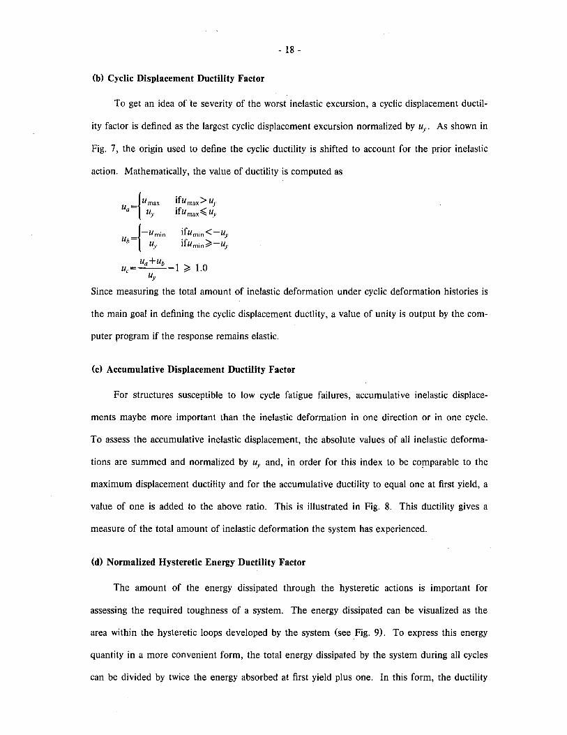
(b) Cyclic Ductility Factor .......................................................................................... 18

(c) Accumulative Displacement Ductility Factor ....................................................... 18

(d) Normalized Hysteretic Energy Ductility Factor .................................................... 18

(e) Comments on Ductility Factors .... ...... ... ... ......... ....... ... ....... ........... ... ......... ...... .... 19

4.3 Number of Yield Events, Yield Reversals and Zero Crossings ................................. 20

4.4 Maximum Response Displacements, Velocities and Accelerations ........................... 21

(a) Displacement ........................................................................................................ 21

(b) Velocity ................................................................................................................ 22

(c) Acceleration ...... ... ... ...... .... ...... ... ....... .... ......... ... ... .... ... .......... .... ..... ....... ..... .... ... .... 23

4.5 Energy Indices ........................................................................................................... 23

5 RESPONSE SPECTRA .. ... ... ...... ....... ... ... .... .......... ...... ... ... .... ... .... .... ......... ......... ... ... ... ... ... 24

5.1 Introduction ............................................................................................................... 24

5.2 Elastic Response Spectra .................................................... :....................................... 24

5.3 Inelastic Response Spectra ......................................................................................... 25

5.4 Construction of Response Spectra Using Computer Program ................................... 27

6 EXAMPLES.. ... ... ........ .......... ... ... ... .... .... .......... .... ...... ... .... ...... ........ ... ... ... ... ... .... ... ...... ...... 28

6.1 Introduction ............................................................................................................... 28

6.2 Shock Spectra ............................................................................................................. 28

6.3 Response Time History for Seismic Excitation .......................................................... 30

6.4 Inelastic Spectra ......................................................................................................... 31

6.5 Comparison of Response Indicies .............................................................................. 33

6.6 Evolutionary Spectra .................................................................................................. 35

7 CONCLUSIONS 37

REFERNCES ........................................................................................................................ 38

-v -

FIGURES .............................................................................................................................. 41

APPENDIX A: PROGRAM INPUT AND OUTPUT ........................................................ 71

A.l Input Specification ..................................................................................................... 71

A.2 Output ....................................................................................................................... 75

APPENDIX B : EQUIVALENT SINGLE-DEGREE-OF-FREEDOM SYSTEMS ............... 77

- 1 -

1 INTRODUCTION

1.1 Introductory Remarks

Buildings and other structures are often designed to respond inelastically when they might

be subjected to rare and unusually intense dynamic loads during their service life. This results

in considerable economic savings relative to designing for such loading on an elastic basis.

Such structures, however, must be designed, detailed and constructed to develop the required

inelastic deformations. When this is done properly, the structures will sustain the dynamic

loading with local damage but without collapse.

This design philosophy is often adopted in design of conventional earthquake-resistant

buildings and of impact- or blast-resistant structures. However, inelastic dynamic response is

complex and difficult to predict using conventional design and analysis methods based on elastic

dynamic behavior (10). Consequently, it is desirable to have design-oriented analytical tools

capable of accounting for the inelastic dynamic response of structures.

General purpose, finite element analysis, computer programs have been developed to

predict the inelastic dynamic response of two- and three-dimensional assemblages of structural

components [1,2,9,11,13,14,20] While such programs are useful in assessing the reliability of a

final design where the geometry and member properties are known, they are generally unsuit­

able for preliminary design. In the initial stages of design little information is available regard­

ing the structure's mechanical or dynamic characteristics. The designer in this case needs basic

guidance in selecting the overall stiffness and strength of a system in order to limit its inelastic

deformations to accceptable levels. Alternatively, the designer may wish to quickly assess the

sensitivity of the overall response of a proposed structure to uncertainties in its mechanical and

dynamic characteristics or to different excitations. General purpose programs can provide little

guidance in such cases.

Fortunately, it may be feasible to represent certain multiple-degree-of-freedom structures

as equivalent single-degree-of-freedom systems [16,21,22,23 and Appendix B). In this case, a

- 2 -

variety of parametric studies can be easily and economically performed using simple structural

models. To facilitate such analyses and the development of general design guidelines, it is

desirable to have a computer program capable of efficiently computing the inelastic response of

such structural models to various dynamic excitations.

1.2 Objectives And Organization

The objectives of this report are to describe a computer program written to analyze the

inelastic responses of viscously damped single-degree-of-freedom systems to either base input

accelograms or direct external load inputs (Fig. 1) and to discuss various methods of developing

design aids based on computed inelastic response. The computer program has been written to

allow the user to conveniently obtain detailed information regarding the inelastic response of a

system and to study systematically the effect of variations in the mechanical and dynamic chara­

teristics of the system and of different excitations.

In Chapter 2, the governing equations of motion for the systems considered are described,

and normalized forms of these equations are derived to illustrate the generalization of the com­

puted responses for a particular system to a family of related systems. The numerical method

used in the program is also described in that chapter with a brief discussion on the accuracy and

stability of the method. Section 2.3 describes the self-adjusting time step scheme adopted in

the program to solve the equations of motion. This method reduces the number of times steps

needed in numerically integrating the equations of motion and automatically controls the accu­

racy of the solution when inelastic events occur.

The two nonlinear force-deformation models incorporated in the program are described in

Chapter 3. These hysteretic idealizations, the bilinear and stiffness degrading models shown in

Fig. 2, are commonly used to analyze many types of structures. However, they are relatively

simple compared to the inelastic behavior exhibited by some types of structures. The use of

seperate subroutines for state determination with each model makes it convenient for the user

to add additional hysteretic models. The last section of Chapter 3 includes a discussion of the

application of the available hysteretic models to account for P-Delta effects due to gravity loads.

- 3 -

In many cases, it is infeasible to inspect the entire response history and a few numerical

indicies are desirable to summarize the response. In Chapter 4, various response indicies to

quantify inelastic response are discussed. The response indices discussed and incorporated in

the program include maximum response displacement, residual displacement, displacement duc­

tility, cyclic ductility, accumulative displacement ductility, normalized hysteretic energy ductil­

ity, number of yield excursions and yield reversals, number of zero crossings, and various

energy indices.

Development of design guidelines for inelastic systems by means of response spectra is

discussed in Chapter 5. The capability of the computer program in generating different kinds of

response spectra is discussed. The program can automatically compute the responses of sys­

tems obtained by permuting all combinations of user-specified lists of periods, yield strengths

and damping values. Alternatively, the user can list the specific combinations of these parame­

ters to be analyzed. These features are useful in constructing constant strength, constant ductil­

ity and other types of response spectra described in Chapter 5.

Examples of using the computer program for generating responses of single-degree-of­

freedom systems and response spectra are given in Chapter 6. Observations regarding inelastic

behavior of structures are also offered. Conclusions and recommendations are offered in

Chapter 7.

In Appendix A, program input specification and output are discussed, and in Appendix B,

modeling of multiple-degree-of-freedom systems by single-degree-of-freedom systems is dis­

cussed.

- 4 -

2 SOLUTION OF EQUATIONS OF MOTION

2.1 Basic Form of Equation

As mentioned in Chapter 1, the program calculates the response of viscously damped,

inelastic, single-degree-of-freedom systems. For a system subjected to an external forcing func-

tion (see Fig. 1), the governing equilibrium equation at time t is

Mu (t}+CU (t}+R (t}=P(t) (1)

where M is the mass of the system, C is the system's damping coefficient, R (t) is its restoring

force and P (t) is the load acting on the system. As shown in the Fig. 1, the displacement of

the system with respect to its fixed base is denoted as U (t).

In the case of horizontal earthquake ground motion excitations (Fig. 1) we may write Eq.

1 in the form:

Mu (t )+Cu (t)+ R (t )=-MUg (t) (2)

where M, C ,R (t) are the same as before. In this case, U (t) denotes the displacement of the

system relative to the ground and ug (t) is the displacement of the ground relative to a fixed

reference axis.

By comparison of Eqs. 1 and 2, one can note that the equation of motion for a seismically

excited system is the same as that for an externally loaded system if the load P (t) equals

-MUg (t). However, the precise meaning of U (t) in each case must be remembered. When

Eq. 1 is applied to a seismically excited system, U (t) represents the displacement of the system

with respect to an accelerating base and the total displacement is v (t) = U (t)+ ug (t); however,

when the equation is applied to an externally loaded system, U (t) also represents the total dis~

placement of the system since the base is fixed.

2.2 Normalized Form of Equations of Motion

Although Eqs. 1 and 2 can be solved directly for the response of a particular system, it is

frequently desirable to express these equations in a normalized form. In this manner, the

specific parameters that influence response can be more readily identified. In addition, the

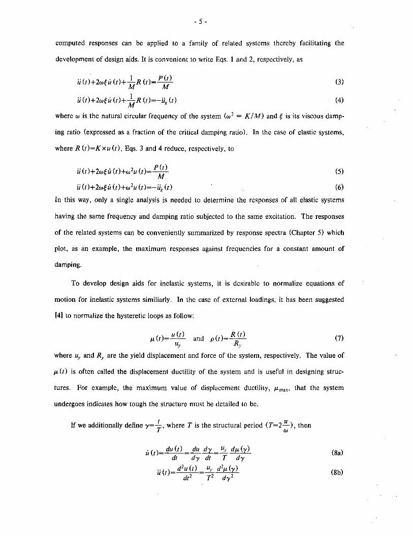
- 5 -

computed responses can be applied to a family of related systems thereby facilitating the

development of design aids. It is convenient to write Eqs. 1 and 2, respectively, as

ii(t)+2wgu(t)+ 1,R(t)=P1;)

ii (t)+2wgu (t)+ 1,R (t)=-iig (t)

(3)

(4)

where w is the natural circular frequency of the system (w 2 = K / M) imd g is its viscous damp-

ing ratio (expressed as a fraction of the critical damping ratio). In the case of elastic systems,

where R (t)=Kxu (t), Eqs. 3 and 4 reduce, respectively, to

ii (t)+2wgu (t)+w 2u (t)= P t) ii (t)+ 2wg u (t )+w2u (t )=-iig (t)

(5)

(6)

In this way, only a single analysis is needed to determine the responses of all elastic systems

having the same frequency and damping ratio subjected to the same excitation. The responses

of the related systems can be conveniently summarized by response spectra (Chapter 5) which

plot, as an example, the maximum responses against frequencies for a constant amount of

damping.

To develop design aids for inelastic systems, it is desirable to normalize equations of

motion for inelastic systems similiarly. In the case of external loadings, it has been suggested

[4] to normalize the hysteretic loops as follow:

() u (t) R (t) p, t =-- and p (t}=--

uy Ry (7)

where uy and Ry are the yield displacement and force of the system, respectively. The value of

p, (t) is often called the displacement ductility of the system and is useful in designing struc-

tures. For example, the maximum value of displacement ductility, P,mm that the system

undergoes indicates how tough the structure must be detailed to be.

If we additionally define y= ~, where T is the structural period (T=2: ), then

u (t)= du (t) = du !!.:L=!!L dp, (y) dt dy dt T dy

(8a)

ii (t) d 2u (t) uy d 2p, (y) df2 T2 dy2

(8b)

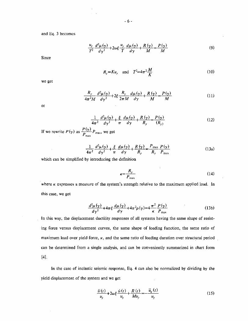
and Eq. 3 becomes

Since

we get

or

- 6 -

R Ku and r 2=47T2 M Y= Y K

1 d2fJ- (y) + ~ dfJ- (Y) +B.hl=.fJ.rl

47T 2 dy2 7T dy Ry (Ry)

If we rewrite P (y) as ~ (Y) P max, we get . max

_1_ d2fJ- (Y) +~ dfJ- (Y) +B.hl= P max.fJ.rl

47T2 dy2 7T dy Ry Ry P max

which can be simplified by introducing the definition

Ry K=--

Pmax

(9)

(10)

(11)

(12)

(13a)

(14)

where K expresses a measure of the system's strength relative to the maximum applied load. In

this case, we get

d2fJ- (Y) +47T~ dfJ- (Y) +47T2p (y )=4~.fJ.rl dy2 dy K Pmax

(13b)

In this way, the displacement ductility responses of all systems having the same shape of resist-

ing force versus displacement curves, the same shape of loading function, the same ratio of

maximum load over yield force, K, and the same ratio of loading duration over structural period

can be determined from a single analysis, and can be conveniently summarized in chart form

[4].

In the case of inelastic seismic response, Eq. 4 can also be normalized by dividing by the

yield displacement of the system and we get

(15)

- 7 -

Although others [18] have suggested dividing by the peak ground displacement, the above

equation is more useful in assessing the structural behavior for design purposes. Making the

variable substitutions introduced previously and noting that the terms

R (t) =.!S... R (t) =W2 R (t) =W 2p (t) Muy M Kuy Ry

(16)

ug (t) = K ug (t) w 2 MUg (t) (17)

Eq. 15 becomes

ii (t )+2wg,l (t)+w 2p (t )=-w2C;: )Ug (t) y

(18)

As in the case of external loading, it is helpful to define a nondimensional parameter, .,." to

simplify the right-hand side of Eq. 18.

.,., Mu gmax

(19)

which expresses a system's yield strength relative to the maximum inertia force of an infinitely

rigid system. Alternatively, if we define the structure's yielding seismic resistance coefficient,

Cy , such that

(20)

then

(21)

and.,., reveals the strength of the system as a fraction of its weight relative to the peak ground

acceleration expressed as a fraction of gravity. In this case, we get

(22)

which is similiar in form to Eq. 13(b). In this final form, the displacement ductility responses

of all systems having the same natural frequency, the same hysteretic characteristics and the

same strength over inertia force index (.,.,) subjected to ground motions having the same shape

can be determined from a single analysis and can be used to summarize the ductility responses

of a family of systems in an efficient way (see Chapter 5).

- 8 -

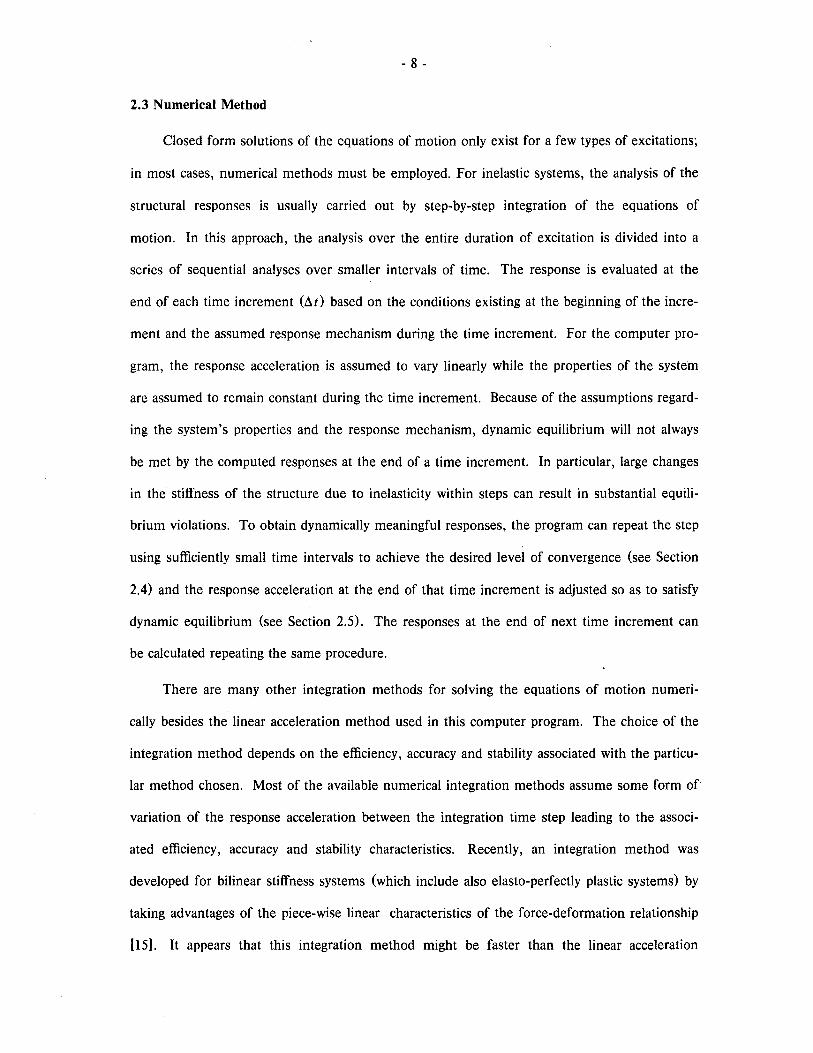
2.3 Numerical Method

Closed form solutions of the equations of motion only exist for a few types of excitations;

in most cases, numerical methods must be employed. For inelastic systems, the analysis of the

structural responses is usually carried out by step-by-step integration of the equations of

motion. In this approach, the analysis over the entire duration of excitation is divided into a

series of sequential analyses over smaller intervals of time. The response is evaluated at the

end of each time increment (~t) based on the conditions existing at the beginning of the incre­

ment and the assumed response mechanism during the time increment. For the computer pro­

gram, the response acceleration is assumed to vary linearly while the properties of the system

are assumed to remain constant during the time increment. Because of the assumptions regard­

ing the system's properties and the response mechanism, dynamic equilibrium will not always

be met by the computed responses at the end of a time increment. In particular, large changes

in the stiffness of the structure due to inelasticity within steps can result in substantial equili­

brium violations. To obtain dynamically meaningful responses, the program can repeat the step

using sufficiently small time intervals to achieve the desired level of convergence (see Section

2.4) and the response acceleration at the end of that time increment is adjusted so as to satisfy

dynamic equilibrium (see Section 2.5). The responses at the end of next time increment can

be calculated repeating the same procedure.

There are many other integration methods for solving the equations of motion numeri­

cally besides the linear acceleration method used in this computer program. The choice of the

integration method depends on the efficiency, accuracy and stability associated with the particu­

lar method chosen. Most of the available numerical integration methods assume some form of

variation of the response acceleration between the integration time step leading to the associ­

ated efficiency, accuracy and stability characteristics. Recently, an integration method was

developed for bilinear stiffness systems (which include also elasto-perfectly plastic systems) by

taking advantages of the piece-wise linear characteristics of the force-deformation relationship

[15]. It appears that this integration method might be faster than the linear acceleration

- 9 -

method, particularly for stiff structures. However, because this computer program is oriented

toward generating and obtaining detailed information regarding response (the various reponse

indicies which will be discussed in Chapter 4), considerable amount of effort is spend in com­

puting these response indicies besides integrating the equation of motion. Consequently, it is

believed that the efficiency of the integration methods in solving the equation of motion is not

a very critical factor in overall efficiency of the computer program. For ths reason, the more

commonly used linear acceleration method is adopted for this computer program.

The normalized forms of equations of motion are useful in illustrating the applicability of

the responses of a particular system to a family of related systems. However, in the computer

program the actual numerical solution of the equations of motion are obtained using the origi-

nal Eqs. 1 and 2. This permits calculations to be performed for a particular system. However,

if desired, input can be specified in terms of the normalized variables indicated previously.

At any instant of time t, Eqs. 1 and 2 can be written as

Mti (t)+CU (t)+R (t)=P(t) (23)

where P (I)=-Mtig (I) for seismically excited systems. While at t + I1t they are (assuming

that the time increment is small enough such that the system's properties remain constant)

Mti (t+l1t)+Cu (t+l1t )+R (t+I1t)=P (t+I1t)

Subtracting the equations, we get

and denoting

M[ii (t+I1I)-ii (I) ]+C [u (t+11t )-u (t )]+ [R (t+I1t)-R (t)]

= [P (t+I1t)-P (t)]

l1ii (I)=ii (t+l1t )-ii (t)

l1u (I)=u (t+l1t)-u (t)

l1u (t )=u (t+l1t )-u (t)

I1R (t)=R (t+l1t)-R (t)

I1P (t )=P (t+I1t)-P (I)

Eq. 11 reduces to

(24)

(25)

(26a)

(26b)

(26c)

(26d)

(26e)

(27)

- 10 -

If 1:.R (t) is denoted as K T1:.u(T), the Eq. 27 becomes

(28)

where KT is a tangent stiffness of the structure between times t and t+ 1:.t, (if KT is assumed

constant during a step). This last equation together with the assumption of linearly varying

acceleration is used to obtain the incremental acceleration, 1:.U (t), along with 1:.u (t) and 1:.u (t).

The actual values of the displacement, velocity are obtained by

u (t+1:.t}=u (t}+1:.u (t)

U (t+1:.t)=u (t)+1:.u (t)

(29a)

(29b)

Instead of calculating acceleration in similiar manner, the actual acceleration is calculated based

on Eq. 14, Sec 2.5, to correct any equilibrium violation. For ground excited structures,

v(t+1:.t) = u (t+1:.t) + ug (t+1:.t). For more details on the numerical integration, see Chapter

8 of Dynamics of Structures [7].

The accuracy and stability of the integration method is of important concern. The linear

acceleration method used is only conditionally stable. That is, for elastic systems, results may

diverge rapidly from the true solution if the integration time step· exceeds the period of the sys-

tern divided by 7T [7]. Stability limits have not been established for inelasitc systems. For

accuracy of the integration method, a time increment not exceeding one tenth of the structural

period is a good rule of thumb [7] for elastic systems. For inelastic systems changes in stiffness

within a step can result in equilibrium violations which must be accounted for to prevent insta-

bility or divergence from the correct solution. Two methods to prevent this are discussed in

the next two sections.

2.4 Time Step Selection

One of the features of the program is the use of a varible time increment (M). One

method for minimizing equilibrium violations due to stiffness changes within a step is to use a

very small 1:.t. This results in a large number of incremental calculations and it is difficult to

know a priori what the time increment should be to achieve the desired level of accuracy. By

varying the time increment, the number of steps (calculations) required can be reduced while

- 11 -

maintaining the desired level of accuracy.

At the beginning of each time step, denoted as time t, a new time increment (at) is

selected based on four criteria. The first criterion requires that at should never exceed aT

which is specified by the user during input. This quantity aT should be selected to achieve the

desired accuracy if the system were to respond elastically.

The second criterion is that at should never be more than the time it would take to reach

the next excitation digitizaton point (these digitizaton points refer to the discretization of a phy­

sically continuous event - the ground movement or the loading on the structure). Thus, the

program will consider the actual record as input, unlike methods which modify the input by

"clipping" peaks in records originally digitized at unequal intervals or at intervals different from

those used in the analysis.

The third criterion is that at should never be more than the time it would take to reach

the next output time specified. The computed responses can be output at time intervals that

are specified by the user in input as a fraction of aT.

The last criterion concerns the convergence of the results when stiffness changes. Fig. 3

shows instances where the computed responses "overshoot" when the stiffness changes. The

solid lines in the figures represent the paths followed by the computed responses when conver~

gence tolerances are met. The dashed lines represent the correct paths the responses should

have taken. To prevent excessive "overshoot" error, convergence tolerances can be specified by

the user. Overshooting also modifies the shape of the hysteretic curves as seen in Fig. 3.

A convergence tolerance, TCONV, can be specified to minimize the amount of overshoot

and the reSUlting distortion of hysteretic curve. Convergence tolerance is checked when the

system yields, unloads from a yielded state, changes from a reduced stiffness state to another

stiffness state for a stiffness degrading model (defined in Section 3.3), or changes stiffness while

crossing the displacement axis during a step for a stiffness degrading model.

These checks are illustrated in Fig 3. In general, the overshoot convergence tolerance is

assumed to be satisfied in each case if the displacement at the end of a step during which a

- 12 -

change in stiffness occurs does not differ by more than TCONVx uy from the displacement at

which the stiffness should have changed. The user can select the value of TCONV to achieve

the desired level of convergence.

If the convergence tolerance is not met, the step is discarded and the program returns to

time t to repeat the calculation again with a smaller time increment. In the program, the step is

reduced by a factor of 10. With such a reduction in the time step, the repeated time step may

not encounter a stiffness change. In that case, the reduced time step is used for all subsequent

steps until the change in stiffness is again encountered. If the convergence tolerance is satisfied

for the reduced time step, the program continues but reverts to the original time step selection

procedure. If the tolerance is still violated, the program disregards the very last time step and

starts from the beginning point of that step using a time step one tenth of the last one (i.e., one

hundredth of the original). This process is repeated until the tolerances are satisfied or the

time step is reduced 5 times without convergence at which time the program stops and notifies

the user of the failure for convergence in the program output. The variable time step algorithm

is illustrated in Fig. 4.

In summary, the current time increment actually used must meet the following four cri-

teria:

(1) It does not exceed aT

(2) It does not exceed the time it takes to reach the next excitation digitization point

(3) It does not exceed the next output time specified

(4) Convergence tolerance is met when applicalbe.

The first three criteria for selecting the time increment are checked before the step

begins; while the last criterion is checked at the end of the step.

2.5 Equilibrium Correction

When equilibrium violations are detected by the program and the user specified loading

and unloading tolerances are satisfied, the program automatically imposes equilibrium by

- 13 -

modifying the acceleration at the end of the step [7]. This is done using the equation

ii(t+At) P(t+At}-Cu (t+At)-R (t+At) M

(30)

- 14 -

3 STIFFNESS MODELS

3.1 Introduction

Two of the more commonly used nonlinear force-deformation models have been imple­

mented in the program and are described in this chapter. The types of structures that are found

to be adequately represented by these hysteretic idealizations are also discussed.

The effects of gravity loads result in changes in stiffness and hysteretic behavior of a sys­

tem. In this chapter, the effects of gravity loads on the two force-deformation models men­

tioned in Sections 3.2 and 3.3 are examined.

3.2 Bilinear Stiffness Model

Bilinear models are frequently used in modeling structures that exhibit stable and full hys­

teretic loops. The bilinear stiffness model is defined by three parameters: the yield point, ini­

tial stiffness, and the post-yield stiffness. The bilinear model is graphically shown in Fig. 2a.

Notice that the yielding always occurs on the two dashed lines - the yielding envelop curves,

and the system always unloads with the initial stiffness until it reaches one of the two yielding

envelop curves. The elastic and elasto-perfectly plastic models are special cases that can be

considered by using appropriate input values. The post-yield stiffness can be of negative value.

3.3 The Stiffness Degrading Model

Stiffness degrading models of the type incorporated are used commonly to represent rein­

forced concrete structures that do not exhibit substantial degradation due to shear and/or bond

deterioration [6,22]. In these cases, the hysteretic loops would be spindle shaped or pinched

[19,22]. The stiffness degrading model also uses a bilinear envelop curve defined by three

parameters : the yield point, the initial stiffness and the post-yield stiffness. The stiffness

degrading characteristics during load reversals are graphically shown in Fig. 2b. There are two

primary differences between this stiffness degrading model and that proposed by Clough and

Johnston shown in Fig. 5. In the Clough and Johnston model [61, the post-yield stiffness is

- 15 -

assumed to be always zero, while the current stiffness degrading model allows non-zero post-

yield stiffness (either positive or negative). Also, as shown in Fig. 2b, for the current stiffness

degrading model, after the initial yielding, the loading is directed toward the last unloading

point in the direction of motion. The Clough and Johnston model always loads toward the

furtherest unloading point in the direction of motion which can result in unrealistic loops (Fig.

5).

Just like the bilinear stiffness model, the stiffness degrading system will always unload

with the initial elastic stiffness; however, the stiffness degrading system changes its stiffness

when it crosses the displacement axis (zero crossing point) and starts loading in the opposite

direction. There is evidence that the unloading stiffness slope should degrade with cycling and

maximum peak displacement. However, analyses [5] indicate that this degraded unloading

stiffness does not generally have a significant effect on seismic response. After it crosses the

displacement axis, it heads straight toward the last yield point as shown in Fig. 2b.

3.4 Inclusion of P-Delta Effects

Gravity loads can effect the apparent mechanical characteristics of a structure when the

system is displaced horizontally. This geometric nonlinearity is often called the "P-Delta" effect.

The P-Delta effect decreases the system's tangent stiffness by P/L where P is the gravity load

and L is the system's height as shown in Fig. 6.

The P-Delta effects can be incorporated into the program by changing the input for the

primary envelops for the bilinear and stiffness degrading model. When P-Delta effects are con-

sidered, the yield displacement uy remains the same, while the new initial period (To), the ini-

tial stiffness (Ko ), the post-yield stiffness (PKo ), the yield strength (Ry) and 1)-value (1)0) are

changed as follow:

(31a)

(31b)

- 16 -

PK'=PK (1-~) o LKo

(3lc)

R 'y=Ryo (1- L~ ) o

(3ld)

71'=710 (1- Li ) o

(31e)

This does not exactly produce the correct effect on stiffness degrading models. Notice that in

Fig. 6, the "zero crossing" point for the stiffness degrading model should be shifted away from

the displacement axis by the P-Delta effects. This can not be taken into account by the current

version of the computer program. Instead, the program assumes the stiffness changes at the

zero crossing point and follows the dashed path shown in the figure. Although not strictly

correct, the responses calculated this way are probably of sufficient accuracy for most practical

values encountered for P-Delta effects.

- 17 -

4 RESPONSE INDICES

4.1 Introduction

While hysteretic curves and response time histories contain all the information on

response, it may not be possible or desirable to inspect these curves for every system analysed.

Consequently, it is useful to define a few simple indices to characterize the response. The max­

imum displacement ductility is commonly used to describe the response of an inelastic system.

It is especially useful for structures with stable hysteretic loops subjected to impulsive loads.

However, when cyclic inelastic action is likely, other indices may provide additional insight into

the behavior of the system. A number of indicies that have been incorporated in the computer

program are discussed in this chapter.

4.2 Ductility Factors

(a) Maximum Displacement Ductility Factor

Displacement ductility is defined as the maximum absolute value of the displacement

response normalized by the yield displacement of the system. This definition of displacement

ductility gives a simple qualitative indication of the severity of the peak displacement relative to

the displacement necessary to initiate yielding and is illustrated graphically in Fig. 7. A max­

imum displacement ductility less than unity represents elastic response; while a value greater

than unity indicates inelastic response.

For monotonic loading conditions, the maximum displacement ductility factor is a good

index of inelastic deformation; however it does not by itself indicate the amount and severity of

inelastic deformations under cyclic deformation histories. In this case the largest inelastic

deformation in a cycle, the number of yield events and reversals and the total amount of inelas­

tic deformation can be substantially larger than indicated by the maximum displacement. These

factors can be important in structures with limited inelastic dissipation capacities.

- 18 -

(b) Cyclic Displacement Ductility Factor

To get an idea of te severity of the worst inelastic excursion, a cyclic displacement ductil-

ity factor is defined as the largest cyclic displacement excursion normalized by uy. As shown in

Fig. 7, the origin used to define the cyclic ductility is shifted to account for the prior inelastic

action. Mathematically, the value of ductility is computed as

U =Iu max a Uy

Ub=I-Umin Uy

Ua+Ub

Uy

ifu max> Uy

ifumax~ Uy

ifumin<-Uy ifumin~-Uy

1 ~ 1.0

Since measuring the total amount of inelastic deformation under cyclic deformation histories is

the main goal in defining the cyclic displacement ductlity, a value of unity is output by the com-

puter program if the response remains elastic.

(c) Accumulative Displacement Ductility Factor

For structures susceptible to low cycle fatigue failures, accumulative inelastic displace-

ments maybe more important than the inelastic deformation in one direction or in one cycle.

To assess the accumulative inelastic displacement, the absolute values of all inelastic deforma-

tions are summed and normalized by uy and, in order for this index to be cO!llparable to the

maximum displacement ductility and for the accumulative ductility to equal one at first yield, a

value of one is added to the above ratio. This is illustrated in Fig. 8. This ductility gives a

measure of the total amount of inelastic deformation the system has experienced.

(d) Normalized Hysteretic Energy Ductility Factor

The amount of the energy dissipated through the hysteretic actions is important for

assessing the required toughness of a system. The energy dissipated can be visualized as the

area within the hysteretic loops developed by the system (see Fig. 9). To express this energy

quantity in a more convenient form, the total energy dissipated by the system during all cycles

can be divided by twice the energy absorbed at first yield plus one. In this form, the ductility

- 19 -

factor represents the maximum displacement ductility of an equivalent elasto-perfectly plastic

system that dissipates under monotonic loading the same amount of hysteretic energy

(represented by the shaded areas) as the actual system. This is a convenient way of visualizing

this factor.

For elasto-perfectly plastic models, the normalized hysteretic energy ductility factor should

equal the accumulative displacement ductility defined in the previous section. However,

because of differences in computational methods for the two quantities, the results may be

slightly different depending on the converenge tolerance used. Fortunately, for most cases, the

differences in the ductilities are insignificant.

(e) Comments on Ductility Factors

Because ductility factors are attempting to simplify a complex response, they must be used

with caution. In general there is little agreement on the precise definition of ductility and scant

data on the ductility capacity of a structure. Moreover, it must be recognized that the ductility

based on local response (plastic hinge rotation, strain, etc.) will· usually be substantially larger

than those based on displacement.

While the definitions introduced above have precise meanings for the single-degree-of­

freedom systems considered, this is not necessarily so for multiple degree of freedom systems

or structures that do not exhibit definite yield points. However, use of the above definitions

individually and in, particular, by comparing them can give a designer a good idea of the type of

response expected of a system [12]. See the examples in Chapter 6 for a comparison of various

definitions of ductility as applied to several structures.

The various ductility factors introduced have been defined to result in identical numerical

values for a monotonic response excursion. In addition, a value of one or less indicates elastic

response in each case. This overcomes some of the difficulties in comparing values that would

result from other methods of normalizing response [8].

The equations of motion were normalized in Section 2.2 in such a way that the values of

- 20 -

the various ductility factors defined previously will be identical for family of systems having the

same characteristics as described in Section 2.2 and subjected to excitations of the same shape.

However, this does not mean that the displacements or force histories will necessarily be the

same. Fortunately, these parameters can be calculated from the definition of ductility and

knowledge of the system's mechanical characteristics and the intensity of the excitation (see

Section 4.4).

4.3 Number of Yield Events, Yield Reversals and Zero Crossings

In addition to having some measures of the severity of inelastic deformations, it is also

desirable to have information on their frequency. To give an indication of any bias in yielding,

the number of yield excursions in the positive and negative directions are given seperately.

Yielding is defined for these indicies as an excursion on the primary post-yield envelop curve

(dashed lines in Fig. 2). Note, small hysteretic loops for the stiffness degrading model that do

not contact the primary envelop are not counted. The number of yield reversals is an impor­

tant quantity. For example, successive yield events can occur in the same direction. Thus,

several small yield excursion may have the same effect as one large event. To distinguish this

case from cases where cyclic inelastic deformation reversals occur the number of yield reversals

is given as well. The number of yield reversals is defined as the number of times the system

changes from yielding in one direction to yielding in the opposite direction. Again only contact

with the primary yield envelop is counted. Because of the behavior of the stiffness degrading

model is hysteretic on all cycles once yielding has occurred, the number of zero crossing (for

reversals) is also given. This also gives an indication of the mean frequency of the response

which may degrade with inelastic deformation.

The definitions of the number of yield events, yielding reversals and zero crossings are

illustrated in Fig. 11. Note that number of events does not change for systems normalized as

in Section 2.2 subjected to excitations of the same shape.

- 21 -

4.4 Maximum Response Displacements, Velocities and Accelerations

(a) Displacement

In addition to controlling inelastic deformations, it is also frequently necessary to control

the maximum relative displacement of a structure. This is done (1) to control the damages to

the nonstructural elements; (2) to mitigate the adverse consequences of P-Delta effects; (3) to

reduce human perception of motion; (4) to prevent pounding against adjacent structures (or

equipment) and (5) to satisfy prescribed code or other displacement limits. Consequently,

information on the maximum displacements of a system are summarized by the computer pro-

gram.

Although the ductilities computed according to the definitions made in Section 4.2 will be

the same for all systems normalized according to Eqs. 13b and 22, the maximum displacements

may be considerably different. To relate the maximum displacements to maximum displace-

ment ductilities, it is helpful to re-write the definition of the maximum displacement ductility

for seismic excitation as

[ ~2] (32a)

or solving for displacement

U max= uy . I.t max (32b)

or

U =...!Lii . max 2 g max I.t max W

(32c)

From this last equation, we can see that for normalized structures subjected to the same nor-

malized excitation and having the same values of wand '1), the value of U max is proportional to

iig ,even though I.tmax is not. However, '1) and iig are related and Eq. 32b is more useful in max max

practice in determining displacements.

For force excited systems, we can also re-write the definition of the maximum ductility as

U max U max K . U max I.tmax=-u-= R /K P

y y K· max [ K] U max

K Pmax (33a)

- 22 -

or

K U max=JL max K P max (33b)

Again, we can see that for normaized structures having the same values of K and K , the value

of Umax is proportional to the Pmax •

If two systems are normalized such that they develop the same ductility, the displacement

of one can be determined from that of the other using

(34)

This equation is convenient when interpreting the computer output.

(b) Velocity

Maximum total response velocity is important in determining the human perception of

motion and maximum relative response velocity is important in determining the strain rate of

the deformation. Similiar to the maximum response displacement, the maximum total response

velocity and the maximum relative response velocity can be normalized as

(35a)

(35b)

or if the velocities are known for a particular system, they can be related to those for a related

system with the same T/ and w by

when /J- {=/J- i (35c)

and

(35d)

- 23 -

(c) Acceleration

Maximum total response acceleration is important in determining the human perception

of the severity of an earthquake and in design of equipments attached to the structure. Similiar

to the maximum response displacement and the maximum total and relative response velocity,

the maximum total response acceleration can be normalized as

4.7 Energy Indices

.. .. .. Tj .. umax=UyJ..Lmax=Ugmax-2 J..Lmax

w

(36a)

36b)

For ground motion excited systems, the computer program will keep track of the amount

of energy. input, absorbed and dissipated. The amount of input energy can be expressed as the

integral of negative of the sum of the resistance force plus the damping force times the ground

velocity over time. The derivation of this expression is shown in Fig. 12.

Part of the input energy is stored in the system as strain energy. For systems with no

deterioration in unloading stiffness, the recoverable strain energy can be computed as half the

square of the force divided by the initial elastic stiffness. Part of the input energy is stored as

kinetic energy. It can be expressed as one half the product of the response velocity relative to a

stationary reference frame and the mass of the system.

Finally, part of the input energy is dissipated as hysteretic energy and can be computed as

the area within the hysteretic loops developed by the system; and the rest of the input energy is

dissipated as damping energy through the viscous damping mechanism of the system. It can be

expressed, for viscously damped systems, as the integral of the damping coefficient times the

square of the response velocity over time. The time histories and maximum values of these

energy terms maybe output by the computer program if desired (see Appendix A, Section A.l,

Card B.2).

- 24 -

5 RESPONSE SPECTRA

5.1 Introduction

In designing structures, especially in the preliminary stage, one is primarily concerned

with the maximum responses rather than the precise details of the response time histories. To

facilitate design of structures subjected to severe dynamic excitations, it would be helpful to

develop design guidelines which indicate how these peak response parameters vary with the

dynamic, mechanical and damping characteristics of the structure for a particular excitation.

Such guidelines can be easily formulated for single-degree-of-freedom systems using various

options incorporated in the computer program. Various peak response can be tabulated for a

set of user specified combinations of stiffness, strength and damping values. Moreover by tak­

ing advantage of the various methods of normalizing the equations of motion discribed in

Chpater 2, different types of response spectra may be constructed as will be described in this

chapter and illustrated in the next. Once constructed, these spectra can be used to derive the

response of a particular system to a specific type of excitation; to determine the consequences

of different design options; and to identify those combinations of design parameters that satisfy

the response criteria. In addition, various spectra can be combined to derive a composite

design spectra where uncertainties exist as to the precise nature of the excitation.

5.2 Elastic Response Spectra

The peak responses of elastic systems can be conveniently summarized by plots of elastic

response spectra. Stated briefly, an elastic response spectrum is a plot of the maximum

response (maximum response displacement, response velocity, total response acceleration, or

any other response quantity of interest) to a specified load function plotted as a function of

system's period (or frequency). Such plots are possible because, as can be seem from Eqs. 5

and 6 of Section 2.2, the responses of systems subjected to a particular excitation are the same

if they have the same frequency and the same amount of damping. Thus, by solving the equa­

tions of motion for one system with each combinaton of period and damping values of interest,

- 25 -

one has determined the response of all systems with these values of period and damping. It is

convenient to summarize this data as response sepctra in which the maximum responses are

plotted against periods for a constant damping value.

Typical elastic response spectra for a seismic excitaion are shown in Fig. 13 for the 1940

EI Centro earthquake. The maximum responses are plotted in terms of the pseudo-acceleration

(Sa), pseudo-velocity (Sv) and the relative displacement (Sd) in a single graph. Pseudo­

velocity is defined as the product of the natural circular frequency of the system and the rela-

tive response displacement. Pseudo-acceleration is defined as the product of the natural fre-

quency of the system and pseudo-velocity.

Sa=peak relative displacement

Sv=WSd

(37a)

(37b)

Sa=wSv=W2Sd (37c)

When defined this way, it is convenient to take advantage of the relationships existing between

these three quantities to plot them in a four-way log paper, known as tripartite plot, as shown in

Fig. 13.

Elastic response spectra have been widely used in earthquake engineering design [7].

Maximum responses of a single-degree-of-freedom structure subjected to a specific excitation

can be conveniently determined from elastic response spectra if only the natural period and

damping of the system are known. In addition, the sensitivity of the responses to variations in

the period or damping of the system can be easily seen from the spectra. However, the elastic

response spectra for different excitations can be sustantially different. Consequently, for design

response spectra, a variety of excitations representative of those expected at a site should be

considered to obtain a smoothed elastic design response spectra [16]. Methods for doing this

are beyond the scope of this report.

5.3 Inelatic Response Spectra

In cases where only maximum response values are of interest, spectral summarization

similiar to that of elastic response spectra is helpful and efficient in identifying the parameters

- 26 -

effecting the response of structures. Looking at Eqs. 21 and 22 of Section 2.2, the ductility

responses of inelastic systems subjected to a specific excitation are uniquely defined for a

specific combination of damping, period and 1]-value. In design, one is usually interested in

controlling displacement ductility values. Consequently, a useful plot would be to graph Il-max

as a function of period for a constant value of 1] and g. Typically, for a single graph the excita-

tion, damping and hysteretic model are held constant and maximum displacement ductility is

plotted as a function of period (frequency) for specified values of 1]. Usually the curves are

plotted on log-log or semi-log scales. Such inelastic response spectra can be called constant

strength response spectra. Spectra for maximum displacement ductility for an elasto-perfectly

plastic system with 5 percent viscous damping subjected to the north-south component of the

1940 El Centro record are shown in Figs. 20 and 21. To use such spectra, one can determine

the maximum ductility or displacement for a particular system for a structure with a period of 1

second and a yield strength of 10 percent of its weight subjected to this record scaled to 50% g

(1] =0.1I0.5=0.2). The maximum displacement ductility can be read from the graph as 7. In

addition, by applying Eq. 32c, the maximum displacement is

umax=.5(32.2xI2)( (2~}2 }ll-max=6.85 inches

Alternatively, one can specify the maximum ductility for a given period and interpolate

between curves to find the required 1]-value. For example, to limit the same structure to a duc-

tility of 4, one would have to use an 1]-value of 0.3. For 50% g peak ground acceleration, this

corresponds to a yield base shear coefficient of 0.15.

Similiar spectra can be plotted for other response quantities of interests as illustrated in

Chapter 6.

Another useful form of inelastic response spectra involves plotting of 1]-values

corresponding to a constant displacement ductility as a functon of period. This form of inelastic

response spectra might be called constant ductility response spectra. They are constructed using

interpolation between the curves of the constant strength spectra as indicated in the example

above. However, as indicated in Fig. 15 and as pointed out in [17], there can be more than one

- 27 -

1j-value corresponding to a given displacement ductility. For example for period of 0.7 second,

the data in Figs. 20 and 21 results in a relation between JL and T as shown in Fig. 15. It is

recommended to take the larger 1j-value for design.

5.4 Construction of Response Spectra Using Computer Program

The output of the computer program is conveniently organized for constructing elastic

response spectra and constant strength inelastic response spectra. As discussed in Appendix A,

Section A.2, when more than one system is input, various maximum response indices are tabu­

lated to facilitate plotting of response spectra.

Direct derivation of constant ductility response spectra is not incorporated into the com­

puter program. In order to generate the constant ductility response spectra, the user would

have to construct a series of constant strength response spectra, and by interpolation, estimate

the constant ductility response spectra.

Inelastic response is very sensitive to the input excitation, and where uncertainty exists as

to the nature and characteristics of this excitation, design should not be based on spectra

developed for a single excitation. Methods for combining spectra for various types of expected

excitatins to produce a composite design response spectra are beyond the scope of this report.

- 28 -

6 EXAMPLES

6.1 Introduction

Several examples are presented to illustrate the capabilities of the program. Moreover,

observations related to the nature of inelastic response under different loading conditions are

offered. Comparisons of the different response indicies previously defined indicate the complex

nature of inelastic response as well as the usefulness in interpreting response.

6.2 Shock Spectra

When systems are subjected to impulsive type of loading, response spectra can be con-

structed similiar to the more familiar earthquake response spectra. Spectra for impulsive types

of loading, frequently referred to as shock spectra, can be constructed using the computer pro-

gram. For example, consider a load history consisting of a single sine pulse base acceleration

time history of duration td and magnitude iig . Shock spectra are constructed for elasto-max

perfectly plastic systems with no viscous damping. For these spectra, 1)-values ranging from 0.2

through 2.0 were used.

It has been shown in Section 2.2 that for a loading of a particular shape, the maximum

displacement ductility depends only on the 1)-value, the amount of viscous damping and the

~ . parameter T for elasto-perfectly plastic systems [4], and only on the amount of viscous damp-

ing and the parameter t; for elastic system [4,6]. The shock spectra are usually plotted in

t terms of the displacement ductility, J.t, and the nondimensional parameter, ;, for a constant

value of 1). Spectra constructed in this manner can be very useful for design where the

assumed load shape can be anticipated or for qualitatively assessing the potential effects of more

complex inputs consisting of a sequence of simple shapes.

The shock spectra computed for the sine pulse loading are shown in Fig. 16. As would be

expected on the basis of simple elastic shock spectra [7], the 1)-values must be at least slightly

- 29 -

greater than 2, in order for systems to remain elastic throughout the entire spectrum range. As

can be seen from Fig. 16(a), for 1/-values less than or equal to 0.8, displacement ductilities tend

to increase with the parameter t;. For 1/-values greater than 0.8 displacement ductilities ini-

tially increase with t; until a peak is reached (between t; = 1 and 2), and then they decrease

with t;. Moreover, it is seen that displacement ductility becomes increasingly sensitive to the

value of 1/ when td exceeds T.

Another interesting aspect of the response can be assessed from plots of normalized peak

displacement (umaxlUg ) versus tdlT for systems with constant 1/-values. For the case con-max .

sidered, Fig. 16(b) shows that all systems respond identically for small values of tdl T (they all

are elastic in this range); for high tdlT values inelastic structures with low 1/-values respond

more than stronger elastic systems, but for intermediated tdl T values structures with low 1/-

values respond less. Similiar trends have been noted previously [16,18]. Interestingly, the

weakest structures considered (1/ =0.2) develop nearly const.ant maximum displacements

throughout the tdl T range. This is apparently a result of the fact that a very weak but stiff sys-

tern will yield early and respond nearly the same as a very flexible but elastic system.

To assess the consequences of this, Eq. 32c is re-written as

(38)

or taking the logarithm on both sides

I Umax I 2 log U =210gT+log(27T) +logumax+log1/ gmax

(39)

For the shock spectra considered, 1/ is constanLIf umaxlug is taken as a constant (as for max

1/=0.2)

(40)

where A is some constant depending on the value of 1/ and the constant value of umaJUg • max

- 30 -

Thus, for weak systems we would expect displacement ductility to be inversely related to period

(with a slope of 2 on a log-log plot). This general trend can be identified in Fig. 16(a) for 71-

values less than 0.6.

6.3 Response Time History For Seismic Excitation

Response time histories of a single-degree-of-freedom system can be obtained using the

computer program. The response of a system is computed for the 1940 EI Centro (N-S)

record. The system has an initial elastic stiffness of 11 06 kipslin. and a yield displacement of

0.06266 in.. Viscous damping was assumed to be equal to 5 percent of critical. Elasto-perfectly

plastic (EPP) and stiffness degrading (SDM) hysteretic idealizations were assumed for the

structure. No deformation hardening is considered in either case.

Typical results are shown in Figs. 17 through 19. These figures include time histories of

displacement, input energy, recoverable strain energy, hysteretic energy and damping energy.

As can be seen from Fig. 17, the maximum displacement is almost the same for both the

stiffness degrading model and the elasto-perfectly plastic system .. However, the displacement

time history of the SDM system consists of less frequent but larger amplitude oscillations than

those of the EPP system. After about 6 seconds, both systems vibrate about a permanent

deformation of about 0.4 inches and it does not appear as though the maximum displacements

would increase with time after 6 seconds ,especially for the EPP system.

From the energy time histories (Fig. 18), we can see that the SDM system would be sub­

jected to considerably more input energy than the EPP system for the same earthquake. For

both systems most of the input energy is being dissipated through hysteresis loops and the

effects of viscous damping are smaller. The kinetic energy and recoverable strain energy

remain relatively small throughout the response. Unlike the displacement time histories which

stop increasing with time after about 6 seconds, the hysteretic and damping energy increase at

an almost constant rate for both systems. Thus, for systems with limited energy capacity, the

duration of the ground motion may have an important effect on the potential failure.

- 31 -

The hysteretic loops for the two systems are plotted in Fig. 19. The figures show many

cycles of reversed plastification. Much more hysteretic energy is dissipated for the SDM than

the EPP as can be seen visually from the hysteretic loops as well as from Fig. 18.

6.4 Inelastic Response Spectra

Constant strength and constant ductility response spectra were also constructed for the

1940 EI Centro (N-S) record. These spectra were calculated for periods range from 0.1 sec to

1.0 sec at 0.05 sec intervals and then up to 2.0 sec at 0.1 sec intervals. Viscous damping was

again assumed to be equal to 5 percent of critical and an elasto-perfectly plastic hysteretic ideali­

zation was used. For the constant 71-value response spectra, defined in Section 5.2, where vari­

ous response parameters are plotted against period for systems with constant 71-values. The 71-

values range from 0.1 to 1.0. The constant ductility response spectra were constructed by inter­

polating the constant 71-value response spectra and this involved an iterative process. The

required 71-values are refined so that they would not result in computed ductilities more than

one percent different from the desired values. The ductilities considered for the constant duc­

tility response spectra range from 2 to 10.

The response spectra generated are shown in Figs. 20 through 26. All of the spectra are

plotted on semi-log scales, except Fig. 20 which is plotted on log-log scale. Shown in Figs. 20

through 23 are the constant 71-value response spectra based on displacement ductility, cyclic dis­

placement ductiltity and normalized hysteretic energy ductility, in that order; and shown in

Figs. 24 through 26 are the corresponding constant ductility response spectra. For the EPP sys­

tem considered, the accumulative displacement ductility values equal the normalized hysteretic

energy ductility spectra. They are consequently not plotted here. However, for other systems,

they provide valuable additional information and it may be desirable to form spectra based on

this parameter as well.

As can be seen from the constant 71-value spectra (Figs. 20 through 23), the various

response ductility factors tend to decrease with increases in 71-value and with increases in

period. For the constant 71-value displacement ductility and cyclic displacement ductility

- 32 -

spectra, lines of constant Tj occasionally intersect and, in some instances, cross over one

another. This results in weaker systems sometimes requiring less ductility than stronger ones.

These intersections and cross-overs correspond to a sharp drop and a positive slope in the Tj-

value versus displacement graph shown in Fig. 15. This tendency is the consequency of

numerous interrelated factors. The effect of a specific pulse in an earthquake record depends

not only on the factors indicated in Fig. 16 (where this same tendency can be noted in some

cases), but on the system's acceleration, velocity and displacement at the onset of the pulse.

Since these values are very sensitive to prior inelastic action, the effect of a particular pulse may

be greater or less than expected based on the characteristics of the isolated pulse.

From the constant ductility spectra (Figs. 24 and 26), it is observed that the Tj-values for

constant ductility generally decrease with increases in ductility and with increases in period.

Because the constant ductility spectra are constructed by interpolating and refining the constant

Tj-value spectra, it would be expected that, for constant displacement ductility and constant

cyclic displacement ductility spectra, that intersection and cross-over of lines for some period

regions might occur. However, when two or more Tj-values would result in the same ductility

the largest value is plotted when constructing these curves. This is believed to be a conserva-

tive assumption for design and accounts for the effect of uncertainties in modeling on response.

Consequently, the constant ductility curves do not cross over one another.

For the constant strength (Tj-value) spectra of displacement ductility shown in Fig. 20, it

is seen that, on a log-log scale plot, the lines of constant Tj-value decrease with period in an

almost linear fashion, especially for high ductility levels and low values of Tj. Similiar to the

observations in Section 6.2, this observation can be related to how the normalized displace-

U max ments vary with period. It is observed in Figs. 28 that the normalized displacement, ii gmax

varies almost linearly with period with a slope less than 2 on a log-log scale plot. Furthermore,

at larger periods the displacements tend to merge as would be expected. Also, as observed in

Fig. 16 (b), the displacements tend to become nearly constant (independent of period) as the

- 33 -

7)-value decreases. To assess the reason for these observations, one refers to Eq. 40. For the

constant 7)-value plot shown in Fig. 28, 7) is constant. As observed previously, /J- varies

inversely and approximately linearly with period for constant values of 7) on a log-log scale plot.

That is,

loW :::::::-a X log T (41)

where a is a positive constant. Therefore, Eq. 39 can be re-written as

U max log -.. - :::::::(2-a)JogT+A. (42) ugmax

where A. is some constant depending on the value of 7). From Eq. 42, it is obvious why the

U normalized displacement, .. max , would vary almost linearly with a slope less than 2 on a log­

ugmax

log scale plot. Similiar conclusion can be made for the variation of normalized displacement

versus period for constant values of displacement ductility by simply recognizing that /J- is con-

stant and 7) varies inversely and approximately linearly with period on a log-log scale plot.

6.5 Comparison of Response Indicies

Comparisons between the different definitions of ductility factors are plotted in Fig. 27 for

constant 7)-values of 0.8 and 0.2, respectively. By comparison, it is seen that ductilities are con-

siderably larger for the weaker system. As noted previously, all ductility factors generally

decrease with increasing period. The maximum displacement ductility and the cyclic displace-

ment ductility are generally similiar (except for periods between 0.4 and 1.0 seconds) indicating

that inelastic deformations occur primarily in one direction. However, the differences between

displacement ductility and equivalent hysteretic energy ductility are as large as two or three

hundred percent indicating many cycles of load reversals and reversed plastification. More

importantly, this difference varies significantly for different periods [10). This observation is

important for structures sensitive to low cycle fatigue and/or with limited energy dissipation

capacity, since for a structure with a certain 7)-value, the designer not only would have to make

sure the structure is sufficiently ductile to develop the required maximum displacement ductil-

- 34 -

ity, but also tough enough to dissipate the required hysteretic energy without significant degra­

dation of its restoring force characteristics.

From the constant displacement ductility spectra obtained in Section 6.4, normalized

response (as mentioned in Section 4.4) envelopes can also be plotted against periods to facili­

tate the comparison between the different response indicies at a constant displacement ductility.

The envelopes are shown in Figs. 29 through 31 for a displacement ductility of 4. In Fig. 29,

differences between the displacement ductility and other ductility factors are shown. Similiar

observations as those just observed for constant 7]-values are evident again for a constant dis­

placement ductility of 4. That is, for structures with limited energy capacity and/or sensitive to

low cycle fatigue, certain periods are preferable over others. Minimum requirements for struc­

tural toughness occur at periods between 1.0 and 1.5 seconds for this input.

The difference between the displacement ductility and cyclic displacement ductility gives

an indication of the directional distribution of the maximum response. The cyclic displacement

ductility as defined can be as large as twice the displacement ductility (minus one) when the

positive and negative displacements are equal. The cyclic displacement ductility can be as small

as the displacement ductility if the inelastic deformation occurs in only one direction or when

the response is elastic (the trivial case). From Fig. 29, it is seen that the directional distribu­

tion of response is substantially biased in one direction for periods between 0.7 and 1.4 seconds.

Furthermore, it is found that the accumulative displacement ductility (and normalized hys­

teretic energy ductility) are nearly proportional to the cyclic displacement ductility indicating

that there is, for this record, some relation between the energy dissipated and the directional

distribution of maximum response.

In Fig. 30, the variations of the normalized maximum and minimum displacements and

residual displacement versus period are shown for a displacement ductility of 4. Except in a

few cases, the displacement in one direction is significantly larger than in the other direction

indicating again a bias in the inelastic response. It is noted that the pattern of bias in the inelas­

tic response observed in this figure matches closely with the pattern discussed in the preceeding

- 35 -

paragraph. The normalized residual ductility tends to increase with period as seen in Fig. 30.

In addition, normalized residual ductility can be as large as 50% of the peak normalized dis­

placement in some instances. Large residual displacement is undesirable because it may make

structural repair infeasible and can accumulate during severe aftershocks leading to structural

instability.

In Fig. 31, the number of yield events versus period is shown and the trend shows that

for more flexible, longer period structures, the number of yield events decreases as expected.

However, there appears to be an even distribution of positive and negative yield events. This is

in contrast with the directional distribution of maximum displacements where the displacement

in one direction is consistantiy larger than the other direction except in a few cases as shown in

Fig. 30. Thus, the number and magnitude of yield events may not be related. For the EPP

medel, the sum of number of positive yield excursions and number of negative yield excursion

minus the number of yield reservals indicates the number of time the system yielded succes­

sively in one direction only. It can be inferred from Fig. 31 that the number of times the sys­

tem yielded successively in one direction only is about 30% of the number of positive or nega­

tive yield events.

Although comparisions such as those discussed in this section can give much insight into

inelastic response, caution should be exercised in generalizations drawn from a single record. A

statistical study of trends based on realistic structural models and on an appropriately selected

ensemble of ground motion records is required.

6.6 Construction of Evolutionary Spectra

Because the response spectra presented previously relate only the maximum response to

period, the relationship that exists between the response time history and the features of the

excitation time history that cause this response is necessarily absent. One of the ways to incor­

porate the temporal nature of response and to display the relationship between response time

history and excitation time history is through an evolutionary spectrum. An evolutionary spec­

trum is a two dimensional contour plot of the response showing the time of the first occurance

- 36 -

of each level of the contour. Usually the x-axis refers to time and the y-axis refers to period of

the structure.

The evolutionary spectra shown in Fig. 32 are constructed by the computer program. The

systems are assumed to be elasto-perfectly plastic with viscous damping of 5%. The periods are

selected evenly from 0.1 to 1.0 seconds at 0.05 second interval; from 1.1 to 2.0 seconds at 0.1

second interval. The l'/-values used are based on the Newmark-Hall inelastic design response

spectra [16], for a specified displacement ductility of 4. Consequently, actual maximum ductil­

ity demands are not exactly equal to 4 [10]. The excitation used is the 1940 EI Centro (N-S)

record. The response quantity shown in the evolutionary spectra is the equivalent hysteretic

energy ductility. Other response quantities can be used to construct simi liar evolutionary spec­

tra. Pre-determined contour levels are selected corresponding to equivalent hysteretic energy at

0.5 interval from 1.0 to 14.5.

- 37 -

7 CONCLUSIONS

This report describes a computer program for the analysis of inelastic viscously damped

single-degree-of-freedom systems to either support excitations or external loadings. The pro­

gram is best utilitized when used to study the sensitivity of the overall response of a proposd

structure to uncertainties in its mechanical and dynamic characteristics or to variation in excita­

tion. Useful definitions of response quantities are introduced in connection with the various

methods of developing design aids based on computed inelastic response discussed.

The computed responses by the computer program have shown excellent agreement with

results by other computer programs. Improvements and further extension of the computer pro­

gram are possible. For example, inclusion of hysteretic idealizations other than the bilinear and

stiffness degrading models is desirable. Studies on methods for combining response spectra for

different excitations and for normalizing excitations are needed. In addition, studies to assess

methods of applying these methods to systems subjected to biaxial excitations and to complex

multiple-degree-of-freedom systems are needed.

- 38 -

8 REFERENCES

(1) ANSYS, Engineering Analysis Systems Users's Manual, Swanson Analysis system, Inc.,

Pennsylvanis, U.S.A.

(2) Bathe, K.J., "ADINA - A Finite Element Program for Automatic Dynamic Incremental

Nonlinear Analysis," Report 82448-1, Accoustics and Vibration Lavaratory, Department

of Mechanical Engineering, Massachusetts Institute of Technology, 1975.

(3) Bertero, V.V., and Zagajeski, S.W., "Computer Aided Seismic-Resistant Design of Rein­

forced Concrete Multistory Frames," Proceedings of the 6th European Conference on

Earthquake Engineering, Vol. II, Dubrovnik, Yugoslavia, September 1978.

(4) Biggs, J.M., "Introduction to Structural Dyanmics," McGraw-Hill, New York, 1964.

(5) Chen, D. "Spectrum of Ductility for Earthquake Resistant Structure," Technical Report

TR-1, Research Labaratory of Earthquake and Blast Resistant Engineering, Qinhua

University, Beijing, 1980.

(6) Clough, R.W., and Johnston, S.B., "Effect of Stiffness Degradation on Earthquake Ductil­

ity Requirements," Proceedings of Japan Earthquake Engineering Symposil:lm, 1966.

(7) Clough, R.W., and Penzien, J., Dynamics of Structures, McGraw-Hill, New York, 1975.

(8) Goel, S.C., "Response of Multistory Steel Frames to Earthquake Forces," AISI, Bulletin

No. 12, November 1968.

(9) Guendelman-Israel, R., and Powell, G.H., "DRAIN-TABS: A Computer program for Ine­

lastic Earthquake Response of Three Dimensional Buildings," EERC Report 77-08,

University of California, Berkeley, 1977.

- 39 -

(10) Mahin, S.A., and Bertero, V.V., "An Evaluation of Inelastic Seismic Design Spectra,"

Journal of The Structural Division, Proceedings of the Am. Soc. of Civil Engineers, Vol.

107, No. ST9, Sep. 1981.

(11) Mahin, S.A., and Bertero, V.V., "An Evaluation of Some Methods For Predicting Seismic

Behavior of Reinforced Concrete Buildings," EERC Report 75-5, Earthquake Engineering

Research Center, University of California, Berkeley, 1975.

(12) Mahin, S.A., and Bertero, V.V., "Problems in Establishing and Predicting Ductility in

Aseismic Design," Proceedings of the International Symposium on Earthquake Structural

Engineering, St. Louis, August 19-21, 1976, Vol. I.

(13) Mondkar, D.P., and Powell, G.H., "ANSR-I General Purpose Computer Program for

Analysis of Non-linear Structural Response," EERC Report 75-37, Earthquake Engineer­

ing Research Center, University of California, Berkeley, 1975.

(14) Mondkar, D.P., and Powell, G.H., "ANSR-II, Analysis of Nonlinear Structural Response,

Users Manual," EERC Report 79-17, Earthquake Engineering Research Center, Univer­

sity of California, Berkeley, 1979.

(15) Nau, J.M., and Hall, W.J., "An Evaluation of Scaling Methods For Earthquake Response

Spectra," Civil Engineering Studies, Structural Research Series, No. 499, University of

l11inois, Urbana, May 1982.

(16) Newmark, N.M., and Hall, W.J., "Procedures and Criteria for Earthquake Resistant

Design," Building Practices for Disaster Mitigation, Building Science Series 46, U.S.

Department of Commerce, National Bureau of Standard, Washington, D.C., Febuary

1973.

(17) Newmark, N.M., and Riddell, R., "Statistical Analysis of the Response of Nonlinear Sys-

- 40 -

terns Subjected to Earthquakes," Civil Engineering Studies, Structural Research Series,

No. 468, University of Illinois, Urbana, August 1979.

(18) Newmark, N.M., and Veletsos, A.S., "Effect of Inelastic Behavior on the Response of

Simple Systems of Earthquake Motions," Proceedings, Second World Conference on

Earthquake Engineering, 1960.

(19) Park, R., and Pauley, T., Reinforced Concrete Structures, John Wiley & Sons, 1975.

(20) Powell, G.H., "Drain-2D Users Guide," EERC Report 73-22, Earthquake Engineering

Research Center, University of California, Berkeley, October 1973.

(21) Saiidi, M., and Sozen, M.A., "Simple and Complex Models for Nonlinear Seismic

Response of Reinforced Concrete Structures," Civil Engineering Studies, Sturctural

Research Series, No. 465, University of Illinois, Urbana, August 1979.

(22) Saiidi, M., and Sozen, M.A., "Simple Nonlinear Seismic Analysis of RIC Structures,"

Journal of Structural Division, ASCE, Vol. 107, No. ST5, May 1981.

(23) Shibata, A., and Sozen, M., "Substitute-Structure Method for Seismic Design in RIC,"

Journal of the Structural Division, ASCE, Vol. 102, No. STl, Jan. 1976.

(24) Tansirikongkol, V., and Pecknold, D.A., "Approximate Modal Analysis of Bilinear MDF

Systems Subjected to Earthquake Motions," Civil Engineering Studies, Structural Research

Series, No. 449, University of Illinois, Urbana, August 1978.

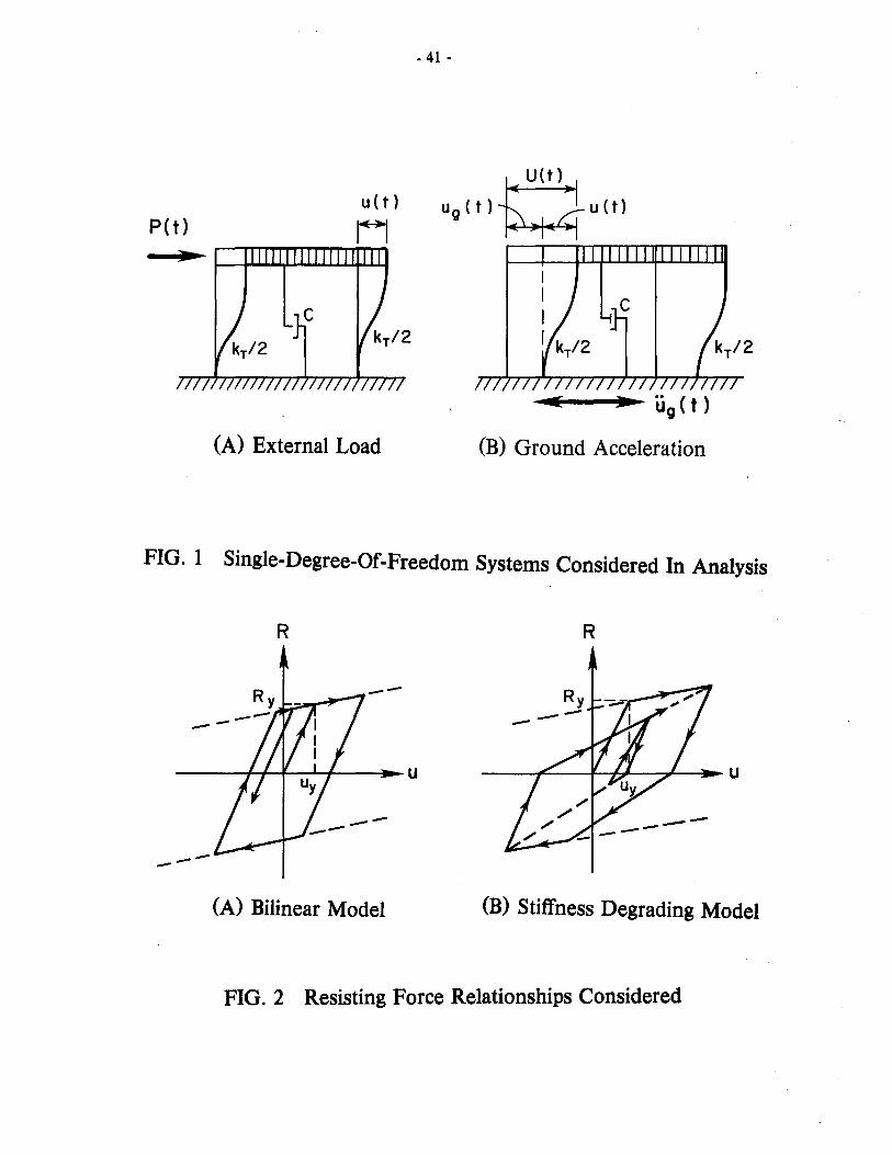
u(t)

P( t} tI

(A) External Load

- 41 -

U( t)

ug(t)~U(t)

(B) Ground Acceleration

FIG. 1 Single-Degree-Of-Freedom Systems Considered In Analysis

R R

---

---(A) Bilinear Model (B) Stiffness Degrading Model

FIG. 2 Resisting Force Relationships Considered

- 42 -

R R

Ry tl

Ry

t,-~ L 8

u u Uy Uy

8<TCONV*uy

(A) Loading To Yield Envelop (B) Unloading From Yield Envelop

R

8 < TCONV * uy

(C) Loading In (D) Unloading In

Stiffness Degrading Model Stiffness Degrading Model

FIG.3 Convergence Tolerances And Modifications Of Hysteretic

Shape Due To Overshoot

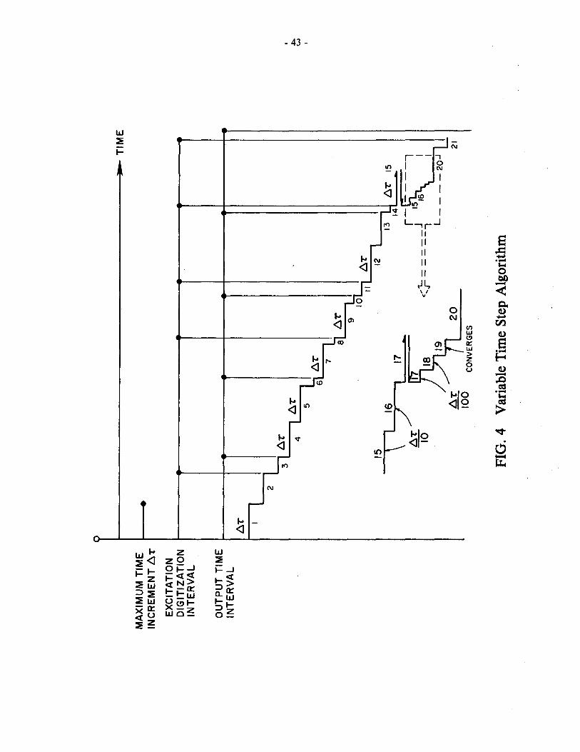
MA

XIM

UM

TIM

E

INC

RE

ME

NT

AT

EX

CIT

AT

ION

D

IGIT

IZA

TIO

N

INT

ER

VA

L

OU

TP

UT

TIM

E

INT

ER

VA

L

o j-----------------------------~----------------~~--TIME

AT

I

15

4 5 16

61 A

T

7

81

AT

9

L 10

AT

I2lU

13

A

T

15

14

In

II

r-

----l

10

) ~1

9 J

15

.... 1

--

_ -

_ _

16

I <

.... .r

--

---l

I

AT

/'

TI

20

1

00

C

ON

VE

RG

ES

L _

_ -

_ 20

.J

FIG

.4

Var

iabl

e T

ime

Step

Alg

orit

hm

21

~

w

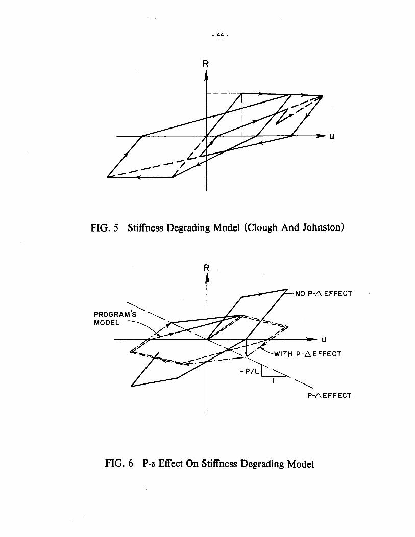
- 44 -

R

FIG. 5 Stiffness Degrading Model (Clough And Johnston)

R

NO P-6 EFFECT

~ PROGRAM'S ~ __ -+-:::-:;&=~~. MODEL ~ _0

.X~

P-6EFFECT

FIG. 6 P-a Effect On Stiffness Degrading Model

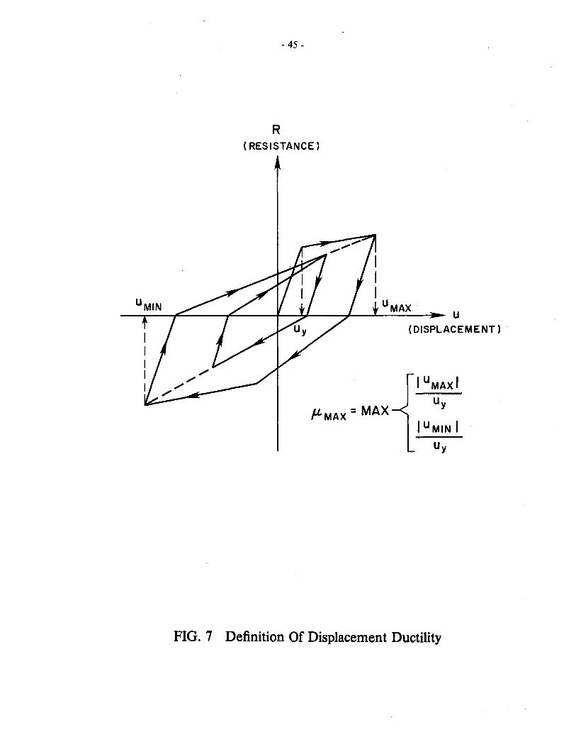
- 45 -

R (RESISTANCE)

__ ~ __ ~~ __ ~~ __ -+ __ ~ __ ~~-L________ U

f-LMAX = MAX

(DISPLACEMENT)

I UMAXI

Uy

I U MIN I Uy

FIG. 7 Definition Of Displacement Ductility

- 46 -

R (RESISTANCE)

--~--~~--------r--L--~~~------~-U

IF UMAX > Uy

IF UMAX ~ Uy

IF UMIN < -Uy

IF UMIN ~ -Uy

CYCLIC DUCTILITY = Ua + ub --- -I ~ 1.0

uy

(DISPLACEMENT)

FIG. 8 Definition Of Cyclic Displacement Ductility

- 47 -

R (RESI STANCE)

/ I

/ ~Uo

----~~--------~~----~~~----~U

/ /

,,...'01(:------- U b ---+--,pJ /

/ /

/

I /

/ /

ACCUMULATIVE DUCTILITY = 1: (upl )j / Uy + I

( I Uo I + I ubi + I Uc I + I Ud I ) = +1 Uy

( DISPLACEMENT)

FIG.9 Definition Of Accumulative Displacement Ductility

- 48 -

R (RESISTANCE)

------~====~~~~~------~(D~IS~P~LA~EMENT)

R/Ry

NORMALIZED HYSTERETIC ENERGY DUCTILITY

( 1 AI 1 + 1 A21 + 1 A 31 ) ~E= +1

Ry Uy

Ry Uy

FIG. 10 Definition Of Normalized Hysteretic Energy Ductility

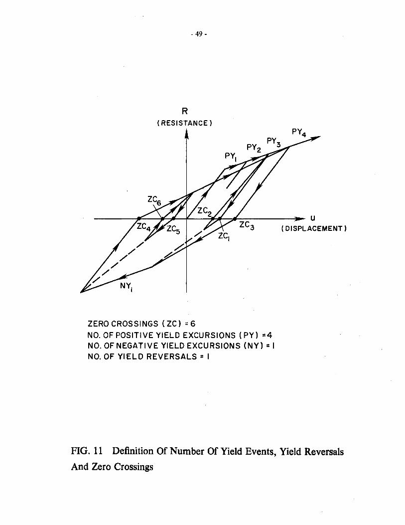
- 49 -

R (RESISTANCE)

------~~~~~~~~~~~------~ U

ZERO CROSSINGS (ZC) = 6

NO. OF POSITIVE YIELD EXCURSIONS (PY) =4 NO. OF NEGATIVE YIELD EXCURSIONS (NY) = I NO. OF YI EL D REVERSALS = I

(DISPLACEMENT)

FIG. 11 Definition Of Number Of Yield Events, Yield Reversals

And Zero Crossings

K/2

- 50 -

~ I ~u(t) .....--....,.....,...-.-----i- - - .., ~-.-.:M~I---__1-__ ~

K/2 / I I

I I

L-______ ~ STATIONARY REFERENCE FRAME

from Figure 1 (b)

M(u (t)+ ug (t) )=- [Cu(t)+ Ku (t)]

Mv(t)=-[Cu(t}+ Ku{.t)]

So the force on the system, according to Newton's Second Law of Motion (F=Ma), is

=-[Cu {t)+Ku {t)]

The work done (equals to the input energy)

input energy= f -[Cu{t)+Ku(t)]x dUg

or

input energy= f -[Cu(t}+Ku(t}]ugdt

FIG. 12 Definition Of Input Energy

u Q)

~ c

r I-u 0 ...J W >

- 51 -

2

I I::---"'B~~:;IL--+

.8~~~~~~~~~--~~~~~~~~~L-~~~~~~

PERIOD (sees)

Fig. 13 Elastic Response Spectra For 0, 2, 5, 10 And 20 Percent

Damping, 1940 El Centro (SOOE) Record

- 52 -

R

----------~~----~~~~~------------~U

U RESIDUAL

URESIDUAL RESIDUAL DUCTILITY = --.:..~--

u y

FIG. 14 Definition Of Residual Displacement Ductility

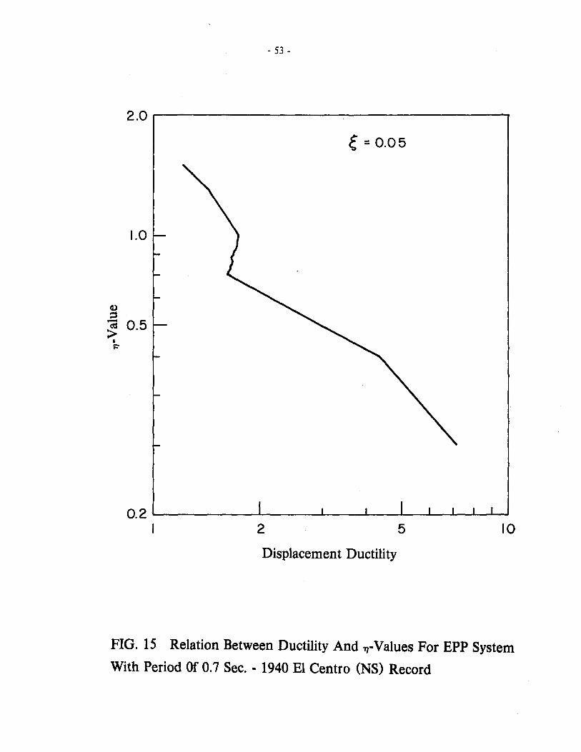
<I) :s

- 53 -

2.0 r---------------------,

e = 0.05

1.0

~ 0.5 I i="

0.2 '---____ -L __ ---1 __ ...1..--_L..---1----L.---'-.--L. .......

I 2 5 10

Displacement Ductility

FIG. 15 Relation Between Ductility And l1-Values For EPP System

With Period Of 0.7 Sec. - 1940 EI Centro (NS) Record

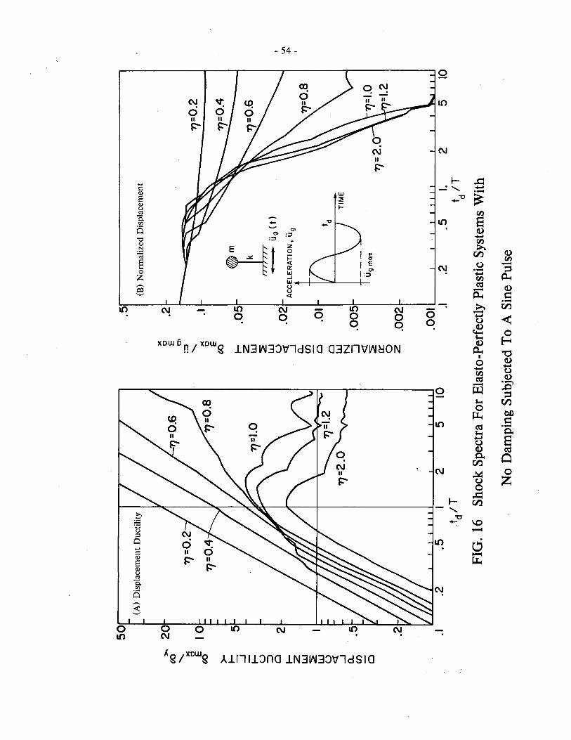
SOr

(A)

Dis

plac

emen

t D

ucti

lity

I 7

7 /

.S

(B)

Nor

mal

ized

Dis

plac

emen

t

x

~ 20~

0

.2

;1//:

1-E

0

1

7] =

0.2

:::

:J

.1 L

~\.

7]=

0.2

.......

E

10

_

_ 1"

\"'_

.,.,=

f'lA

x

(j()

0 E

~

(j()

~

~

.OS

r ...

J z

~

w

u ~

::J

W

-U

g(t

) C

l u

.02

\\

\ \.

'I

V

\ «

ACC~LERATION, u

g .j:

>.

~

...J

Z

a..

w

en

~

Cl

.01

w

u C

l «

w

I \

I T

IME

...

J N

a..

...J

.O

OS

en

« I

I U

g m

alt

Cl

~

0::: 0 z

.00

2

.I .2

.S

2

.00

1

S 10

.I

.2

4S

I. 2

5 10

td

/T

td I

T

FIG

. 16

Sh

ock

Spec

tra

For

Ela

sto-

Per

fect

ly P

last

ic S

yste

ms

With

No

Dam

ping

Sub

ject

ed T

o A

Sin

e Pu

lse

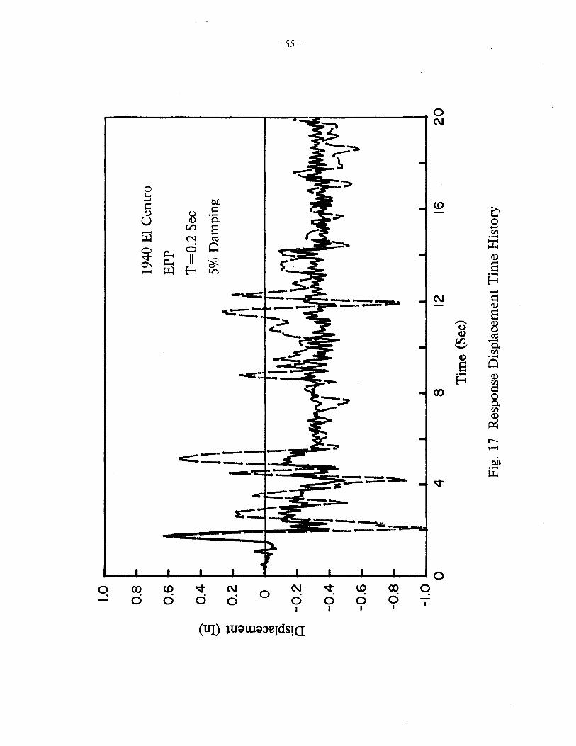
1.0

0.8

0.6

-0

.4

e ......

0.2

c:: Q

) e Q)

CJ

0 tQ

-C. rIl .-

-0.2

0

-0.4

-0.6

-0.8

-1.0

0 4

8 12

Tim

e (S

ec)

1940

El

Cen

tro

EP

P

t=0

.2 S

ec

5% D

ampi

ng

16

Fig.

17

Res

pons

e D

ispl

acem

ent

Tim

e H

isto

ry

20

VI

VI

d -~ '-' >. ~ u = Il.l

- 56 -

1000

800 l-

600 I-

KINETIC AND RECOVERABLE STRAIN ENERGY

400 I-

200 e~'m1l111 ,:J

I- H' J

I I

.h 111ft ~.~V : : : : A~: l(trifd~'GY' :?:: .

: . " . : .. : : : . : . . . . : o

o 4 8 12 16 20

Time (Sec)

(A) Elasto-PerfectIy Plastic

1000 r---------------------------~------------_.

800 I-

600 t-

400 t-

200 t-

o o

KINETIC AND RECOVERABLE

STRAIN ENERGY

:. : : "

LJjn ~:' 4 8

ric f" .... : .:. i:{::::\

. " ': ~ . ~ :, '.

12 16

Time (Sec)

(B) Stiffness Degrading Model

:: '. ::

20

Fig. 18 Energy Time History For Systems With Initial Elastic Period Of 0.2 Sec,

5% Damping And 1)-value Of 0.48 Subjected To 1940 El Centro (NS) Record

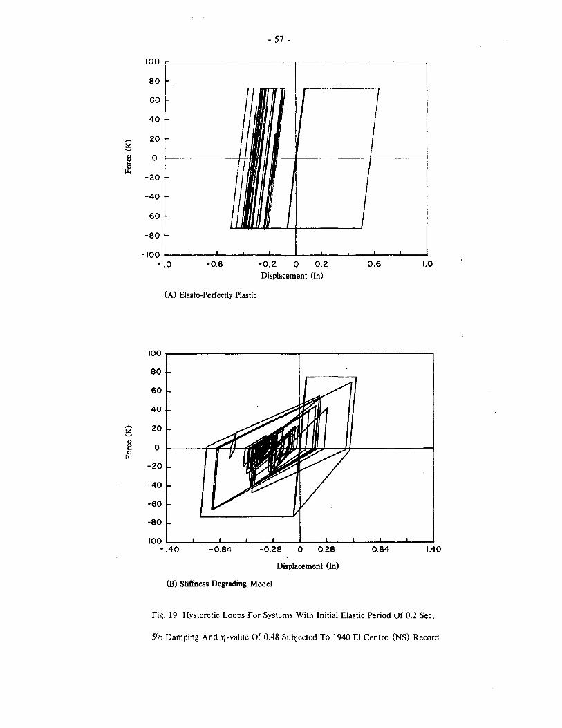
- 57 -

100

80

60

40

Q 20

'-'

8 0 ... &

-20

-40

-60

-80

-100 -1.0 -0.6 -0.2 0 0.2 0.6 1.0

Displacement (In)

(A) Elasto-Perfectly Plastic

100

80

60

40

'""" 20 :oil '-'

8 0 ... 0 ~

-20

-40

-60

-80

-100 -1.40 -0.84 -0.28 0 0.28 0.84 1.40

Displacement (In)

(B) Stiffness Degrading Model

Fig. 19 Hysteretic Loops For Systems With Initial Elastic Period Of 0.2 Sec,

5% Damping And 'I'j-value Of 0.48 Subjected To 1940 EI Centro (NS) Record

- 58 -

6

5 ~ .... . --.- 4 .... (,)

~ 0 .... s:: Cl)

3 e Cl) (,) as -0. fIl .-0

2

o 0.4 0.8 1.2 1.6 2.0

Period (Sec)

FIG. 20 Displacement Ductility Spectra For Elasto~Perfectly Plastic

Systems Of 1)-Values From 0.1 To 1.0 With 5% Damping Subjected

To 1940 El Centro (NS) Record On Log-Log Scale

- 59 -

Period (Sec)

FIG. 21 Displacement Ductility Spectra For Elasto-Perfectly Plastic

Systems Of T/-Values From 0.1 To 1.0 With 5% Damping Subjected

To 1940 EI Centro (NS) Record On Semi-Log Scale

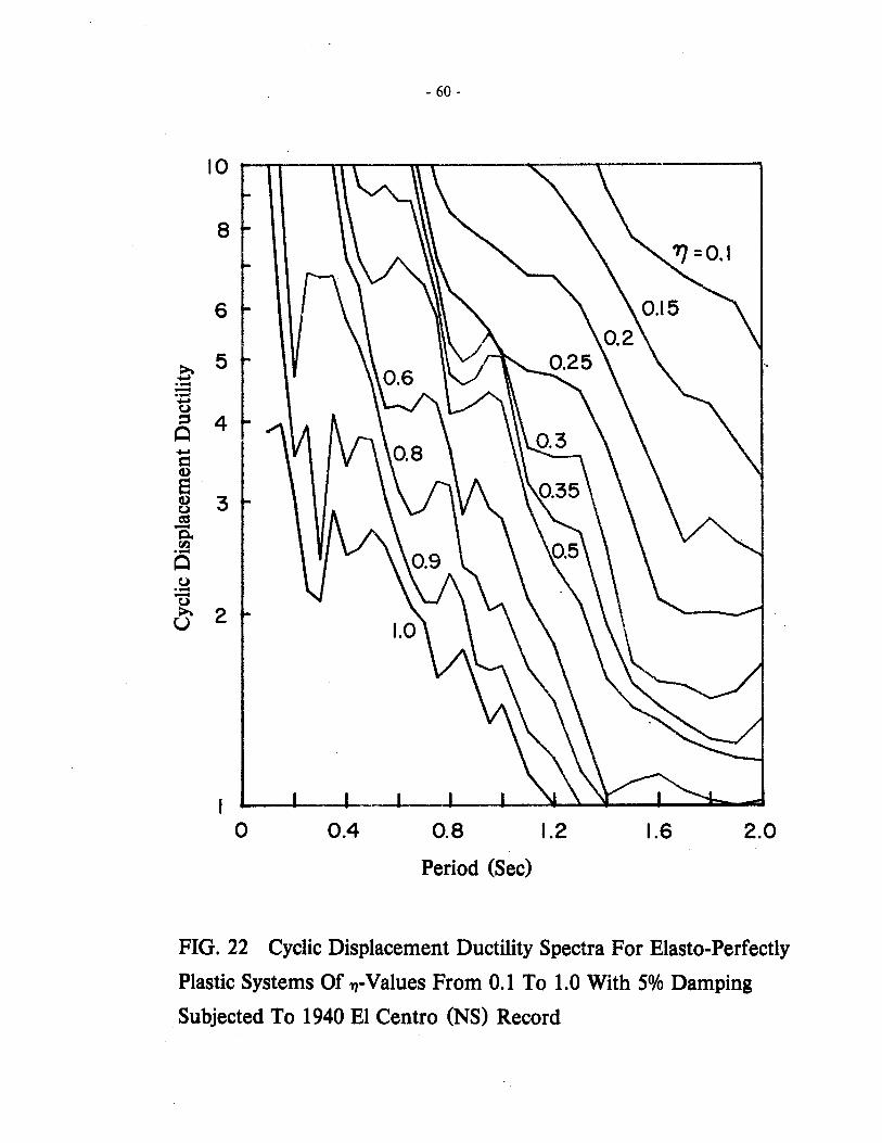
- 60 -

10 ~~--~--~~------~--~--------~

8

6

.e- 5 .--.-..-(,)

~ 4 0 ..-s::= G)

S G) 3 (,) as -0. fIl .-0 (,) .--(,) >. 2 U

1 o 0.4 0.8 1.2 1.6 2.0

Period (Sec)

FIG. 22 Cyclic Displacement Ductility Spectra For Blasto-Perfectly

Plastic Systems Of 1J-Values From 0.1 To 1.0 With 5% Damping

Subjected To 1940 BI Centro (NS) Record

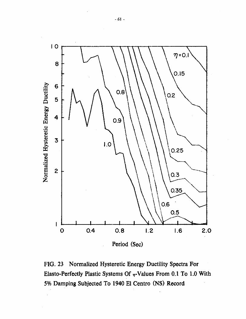
- 61 -

8

~ 6 ~ .--.-~ u ::s 5 0 ~ bO t-4 Q.) 4 Jl u

~ .-~

Q.) t-4 Q.)

3 ~ rIl ~ • ::t:

~ "C Q.) N .--cd

8 2 '--. t-4 0.3 0 Z

I o 0.4 0.8 1.2 1.6 2.0

Period (Sec)

FIG. 23 Normalized Hysteretic Energy Ductility Spectra For

Elasto-Perfectly Plastic Systems Of l1-Values From 0.1 To 1.0 With

5% Damping Subjected To 1940 El Centro (NS) Record

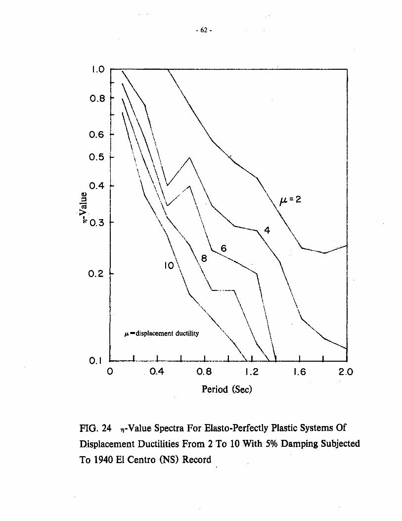
- 62 -

1.0

0.8 ~. I

~~\ 0.6 t 0.5 t '\\' 1\ \ \\ \I 0.4 \\\/'\ co

::s -as > I '~ \ ~0.3 \ \

~\ \8~ 0.2 \ \

\~\ ",,- \

IJ. -displacement ductility ", \

0.1 -1 ___ 1 - 1. __

0 0.4 0.8 1.2 1.6 2.0

Period (Sec)

FIG. 24 1j-Value Spectra For Elasto-Perfectly Plastic Systems Of

Displacement Ductilities From 2 To 10 With 5% Damping Subjected

To 1940 EI Centro (NS) Record

- 63 -

1.0 ,.....-:---------.

Q) 0.4 ~ > I ~

0.3

0.2

0.1 o 0.4 2.0

Period (Sec)

FIG. 25 l1-Value Spectra For Elasto-Perfectly Plastic Systems Of

Cyclic Displacement Ductilities From 2 To 10 With 5% Damping

Subjected To 1940 EI Centro (NS) Record

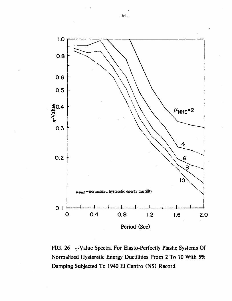
- 64 -

1.0 _----__.....---r-------------.,

0.8

0.6

0.5

gO.4

~ I ~

0.3

0.2

0.1 o

ILNHE-normalized hysteretic energy ductility

1 J I 1 0.4 0.8 1.2 1.6 2.0

Period (Sec)

FIG. 26 ",-Value Spectra For Elasto-Perfectly Plastic Systems Of

Normalized Hysteretic Energy Ductilities From 2 To 10 With S%

Damping Subjected To 1940 EI Centro (NS) Record

>. .... .- -.- .... C

)

~

Q

10 I

I . \

8 I-

.~

L/"

\ \ \ " \ 5

I-\I

\

10

DIS

PL

. D

UC

T.

---

CY

CL.

DU

CT

. 8

-'-'-

NO

RM

. H

YS

T. E

NG

. D

UC

T.

(A)

1/=

0.8

5

"

\ \ \ (B

) 1/

=0.

2 \

" ". -".

:r ~l

\ t

1\ l"

'. \

~' \

\ .

\ \

I .

. \

\ . ~\

.0

4

.- -.- .... C)

3 ~

Q

21

-

01 0

\ \

-'

, \

\ \

2

\_-

\ ~ \ \ ~

---

DIS

PL

. D

UC

T,

--

-C

YC

L. D

UC

T.

--'-

'--

NO

RM

. H

YS

T.E

NG

.DU

CT

I I

I 0.

4 0.

8 1.

2 1.

6 2

.0

o 0

.4

0.8

1.

2 1.

6 2

.0

Per

iod

(Sec

) P

erio

d (S

ec)

FIG

. 27

C

ompa

riso

n A

mon

g D

aisp

lace

men

t D

ucti

lity

, C

yclic

Dis

­

plac

emen

t D

ucti

lity

And

Nor

mal

ized

Hys

tere

tic

Ene

rgy

Duc

tili

ty

Spe

ctra

For

Ela

sto-

Per

fect

ly P

last

ic S

yste

ms

Of

1/-V

alue

s o

f 0.

8 .A

nd

0.2

Wit

h 5%

Dam

ping

Sub

ject

ed T

o 19

40 E

I C

entr

o (N

S) R

ecor

d

0\

VI

- 66 -

0.1 ~-----------------------------------,

..... 5 e G)

~ -C. rJl .-o

"0 G) N .­-as

0.05

e 0.01 1-4 o Z

0.005

0.001 L-______ ~ __ ~ __ ~~~~~~~ ____ ___

0.1 0.2 0.5

Period (Sec)

1.0 2.0

FIG. 28 Normalized Displacements For Elasto-Perfectly Plastic

Systems With 71-Values Of 0.1,0.2,0.4,0.6,0.8,1.0 And 5% Damping

Subjected To 1940 EI Centro (NS) Record

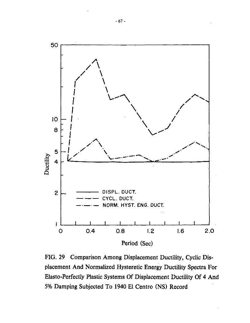
- 67 -

50~----------------------------------~

21- DISPL. DUCT. CYCL. DUCT. NORM. HYST.ENG.DUCT.

I ~~'~~' __ ~1 ___ ~1 __ 1~~1 __ ~1 ___ ~1 __ 1~ __

o 0.4 0.8 1.2 1.6 2.0

Period (Sec)

FIG.29 Comparison Among Displacement Ductility, Cyclic Dis­

placement And Normalized Hysteretic Energy Ductility Spectra For

Elasto-Perfectly Plastic Systems Of Displacement Ductility Of 4 And

5% Damping Subjected To 1940 El Centro (NS) Record

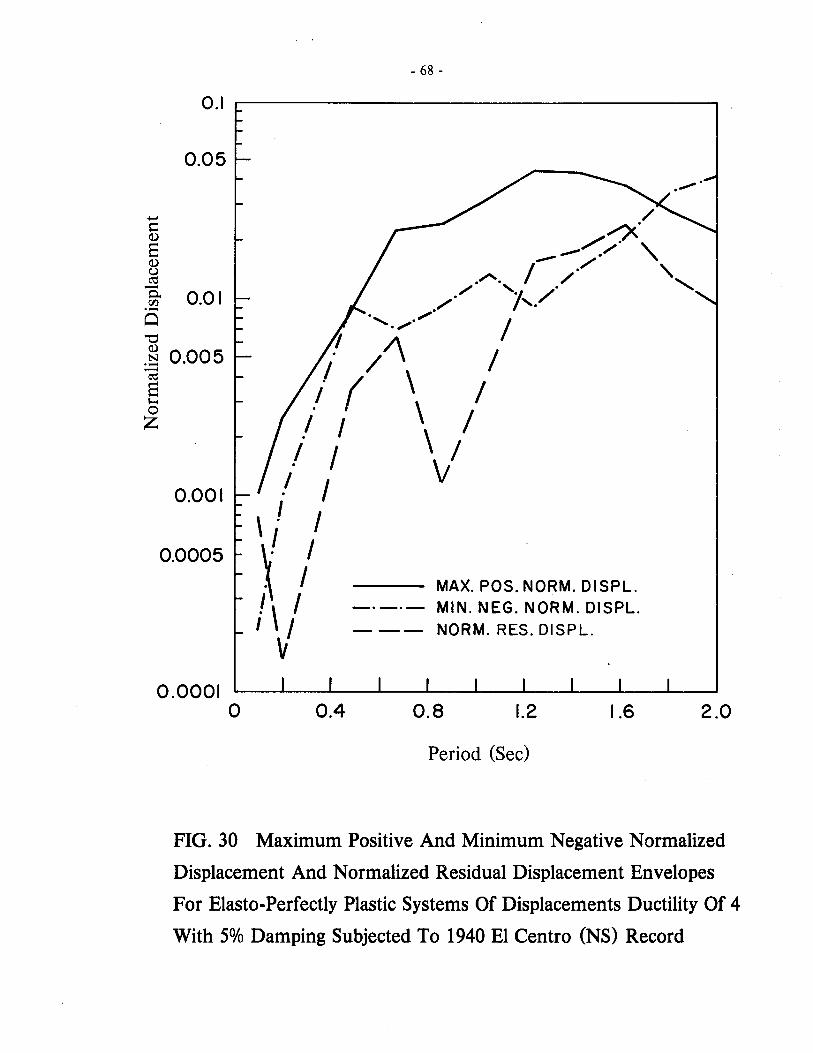
...... o Q)

S Q) u ~ -

- 68 -

0.1 ~----------------------------------~

0.05

/ ....-x. ----~/. "

/ ./ " ~ 0.01

.".... / " ./ './. /' /' I'· .-

....... .,,' / ." Q "0 Q)

.~ 0.005 ? /1\ / / ( \ /

-~ S $-<

o Z

0.001

0.0005

.I I \ / .I I \ /

.I / 'v \! I V I ,\ I ! \ I I I

\I

--- MAX. POS. NORM. DISPL. MIN. NEG. NORM. DISPL.

- -- NORM. RES. DISPL.

0.0001 o 0.4 0.8 1.2 1.6 2.0

Period (Sec)

FIG. 30 Maximum Positive And Minimum Negative Normalized

Displacement And Normalized Residual Displacement Envelopes

For Elasto-Perfectly Plastic Systems Of Displacements Ductility Of 4

With 5% Damping Subjected To 1940 EI Centro (NS) Record

rn ~

s:= a> > ~ "C -a> .-~ c-0 .... a>

.D e ::s Z

20

18

16

14

12

10

8

6

4

- 69 -

.................. , "-'\

\ r'. \ " \ , . . \ \ 1 .

\ . , , ~ \

\

" \ . \ , ,

--- POS. YIELD _._. - NEG. YIELD

1'" "- /

"- II" "- / . \ "- /. "- .

.-._. " I. . /- ' ..

2 - - - YIELD REVERSAL

"

o ~~ __ ~ __ -L __ ~ __ ~ __ L-~~~ __ -L __ ~

o 0.4 0.8 1.2 1.6 2.0

Period (Sec)

FIG. 31 Number Of Yield Events For Elasto-Perfectly Plastic Sys­

tems Of Displacement Ductility Of 4 With 5% Damping Subjected

To 1940 EI Centro (NS) Record

2.0

1.5

-- u w

(J

) - Cl o 1

.0

f-

a::

w

a..

0.5

~

0.1

<!

-Ig

o

\ '1~

1 T

'\

..

. 50

-

1.50

->

tl.oo~

I I

2.0

0.

I ;tt

. /

~? ~

/ ;;::

::::::

Iri(1

~-

::;J~L~

~

~

if. ir

-'

~

~~i~

~ ~W

1,--1

./

~~~

§j -

~ ~I!

I -

-\.

...,

~!L~~iL: .

_

~

. (

-(i

_. :&;~

....

m=

.

J-.

==

...

5 10

15

T

IME

(S

EC

)

Fig

. 32

N

orm

aliz

ed H

yste

reti

c E

nerg

y D

ucti

lity

Evo

luti

onar

y Sp

ectr

um

For

EP

P S

truc

ture

Wit

h 5%

Dam

ping

Sub

ject

ed T

o 19

40 E

l C

entr

o (N

S)

Rec

ord

-..J

o

- 71 -

APPENDIX A : PROGRAM INPUT AND OUTPUT

A.I Input Specification

The program has been used and tested extensively in mainframe computers like CDC

6400 and CDC 7600 and mini-computers like PDP 111780, PDP 111750 and PDP 11170 using

the UNIX operating system. The following input format should be observed when using the

computer program. The variable names indicated are those used in the computer program.

A. JOB TITLE (8AIO) - ONE CARD

columns 1-80 : Information to be printed in the beginning of the output.

B. SYSTEM DEFINITION

Bl. SYSTEM/ANALYSIS INFORMATION (8FIO.O) - ONE CARD

columns 1-10 : XMASS. System's mass. If XMASS is positive, then the program will con­

sider all combinations of the stiffness (or period) listed in Section B4 and the

yield displacement (or 1J-value) listed in Section B5 in calculation of

responses. If XMASS is negative, then the stiffness (or period) and yield

displacement (or 1J-value) will be considered in pairs in the order they are

input. (NOTE: a particular system's mass is not required if 1J-value and

period are specified for the normalized responses of a family of related sys­

tems, and can be made equal to one arbitarily. See Section 2.2)

columns 11-20: PK. Deformation hardening/softening ratio. This ratio should be input as

fraction of the initial elastic stiffness, with zero value permitted for the case

of elasto-perfectiy plastic systems.

columns 21-30: DELTAT. The maximum time increment to be used in the analysis. How­

ever, the program automatically selects smaller time increments to match the

loading interval, the output interval, or to obtain the specified convergence

tolerance when stiffness changes (see Section 2.4)

columns 31-40

- 72 -

XOUT. A multiplier for obtaining output interval for response time his­

tories. The output time interval will be determined as output time interval

= XOUT * DELT AT. To supress response time histories simply use a

sufficiently large XOUT value. (X OUT = 1.0 is the default).

columns 41-50: TCONV. Convergence tolerance. This tolerance can be used to control the

amount of overshoot and distortion of the hysteretic curve shape (see Sec­

tion 2.4). (TCONV = 0.01 is the default)

B2. SYSTEM/ANALYSIS COMMANDS (lOIS) - ONE CARD

columns 1-5 :

columns 6-10 :

NSTIFF. Number of stiffness or periods to be specified. A negative value

for NSTIFF will result in periods being read in Section B4, while a positive

value for NSTIFF results in stiffnesses being read.

NUYP. Number of yield displacements or 'Y/-values to be specified. A nega­

tive value for NUYP will result in 'Y/-values being read in Section B5, while a

positive value for NUYP will result in yield displacements being read.

columns 11-15: NDAMP. Number of damping values to be considered. NDAMP = 1 is the

default.

columns 16-20: ITYPE. Hysteretic model identifier.

ITYPE = 1 - bilinear hysteretic model (default)

ITYPE = 2 - stiffness degrading model

columns 21-25: IENG. Energy computation option.

IENG = 0 - energy computation desired

IENG = 1 - no energy computation desired

Energy computation is made only if the system is excited by ground

motions.

- 73 -

columns 26-30: IPUNeR (output history storage).

IPUNeR = 1 - no output history is desired.

IPUNeR = 2 - the response displacement, resistance force histories are to

be saved either on punched cards or on Tape 1 depending on the value of

JTAPE (columns 31-35).

IPUNeR = 3 - the response displacement, resistance force, energy ductility

and residual ductlity (defined as the residual displacement over the yield dis­

placement, see (Fig. 14) histories are to be saved either on punched cards or

on Tape 1 depending on the value of JTAPE(columns 31-35).

IPUNeR = 4 - response displacement, velocity, acceleration, resistance

force, input energy, kinetic energy, recoverable strain energy, hysteretic

energy, damping energy, energy ductility and residaul ductility histories are

to be saved either on punched cards or on tape 1 depending on the value of

JTAPE (columns 31-35).

columns 31-35: JTAPE. File disposition for option associated with IPUNeR.

columns 36-40

JT APE = 1 when file is to be punched.

JT APE = ° when file is to be written on Tape 1.

IRED. Reading option. If IRED = 0, the information on the first input

card will be repeated on the top of each output page. If the value of IRED

is non-zero, such heading will only appear on the first page of the output.

columns 41-45: JPUNeR. For non-negative value of JPUNeR, the spectra (see Appendix

A, Section A.2) will be punched on cards, otherwise spectra will only be

printed.

columns 46-50: JPRINT. For JPRINT = 0, the spectra will be written on output file. For

non-zero value of JPRINT, the spectra will be written on the output file and

on Tape 7. The purpose of writing spectra on Tape 7 is to enable the user to

- 74 -

dispose the detailed output histories and related summaries and the spectra

tables to different output devices (e.g. microfiche) when only the informa­

tion about the spectra is desired.

B3. DAMPING CARDS (SFIO.O) - AS MANY CARDS AS ARE NEEDED TO ENTER

DATA

Damping values to be considered are expressed as fractions of the critical damping value (

defined as two times the product of system's mass and natural circular frequency).

B4. STIFFNESS OR PERIOD (SF10.0) - AS MANY CARDS AS NEEDED

Whether stiffness or period values are input depends on the sign of NSTIFF as described

in Section B2.

B5. YIELD DISPLACEMENT OR N-VALUE (SFIO.O) - AS MANY CARDS AS NEEDED

Whether yield displacement of 7J-value are input depends on the sign of NUYP as

described in Section B2.

C. LOADING

C1. LOAD CONTROL (2I5,2FIO.O,lOA5) - ONE CARD

columns 1-5 :

columns 6-10 :

KOUNT. Total number of acceleration or external load values to be read.

If KNOUT = 0, then the previous record will be used.

IND. Excitation indicator flag. When IND = 0, the system is excited by

ground motion. When IND = 1, the system is excited by external· loads.

columns 11-20: DT. Time increment between input acceleration or external load values. If

DT is non-zero, the program assumes the excitations input occur at constant

time interval. If DT = 0, pairs of time-acceleration (or pairs of time­

external load) values will be read. The latter case is useful when the excita­

tion is not recorded at equal intervals.

- 75 -

columns 21-30: FACTOR (excitation scaling factor). To scale input ground acceleration or

external loads by a constant FACTOR.

columns 31-80: FMT. Fortran format specification for inputing excitation. The format must

be bracketed within parentheses.

C2. EXCITATION RECORD

As many cards as necessary to read KNOUT number of values according to the specified

format in Section C1).

D. EXECUTION DISPOSITION

0) To terminate execution, place three blank cards after the excitation record.

(2) To proceed to a new problem, repeat data input starting with Card A, but

note that record need not be input again if the same excitation is to be con-

sidered (see Section C 1).

E. STORAGE REQUIREMENT

There are no inherent limits to the number of cases or duration of the record; bowever,

in each case considered, no more than 10,000 blank common can be used. The length of

blank common required for any record can be estimated as

[ DTxKOUNT I

length oj blank common =2xKOUNT+ 8x XOUTXDELTAT+2

+ 15x [NSTIFFxNUYP]+NDAMP+NSTIFF +NUYP+2

A.2 Output

The input information is summarized in a table at the beginning of the output for each

system followed by the time history of the input excitation. When a family of systems are

specified in the input subjecting to an identical excitation, only one excitation time history will

be echoed in the output followed by a series of summaries of the responses of the family of

systems. The computed responses can be presented at two levels of detail depending on the

- 76 -

needs of the user. When complete histories of the responses are desired, the user can specify

in the input complete time histories of the response displacement, the response velocity, the

response acceleration, the input energy, the kinetic energy, the recoverable energy, the damp­

ing energy, the ground acceleration, the ground velocity and the ground displacement. For

input containing more than one structures, seperate sets of time histories will be generated for

each structure defined in the input and for each excitation record specified. Alternatively, the

output will present only summaries of the maximum and the minimum of the above mentioned

responses as well as the times of their occurance.

Following either one of the presentations of the computed responses, a short summary of

the system properties and response envelopes is tabulated. The information in the summary

include the 1J-value of the system, maximum positive and negative displacement ductilities,

cyclic ductility, accumulative ductility, normalized hysteretic energy ductility, number of posi­

tive and negative yield excursions, number of yield reversals, number of zero crossing, residual

displacement, and absolute maximum response acceleration, velocity and displacement.

Whenever the responses of more than one system are computed, a summary of selected

responses of all systems is listed in a seperate table in the order of the computation. This is the

spectra referred to in Appendix A, Section A.I, Card B.2. The responses are the maximum and

minimum displacement ductilities, cyclic ductility, normalized hysteretic energy, accumulative

ductility, the magnitude and the time of occurance of the maximum and minimum displace­

ment normalized by the peak ground acceleration, the residual displacement, the number of

positive and negative yield excursions and zero crossings.

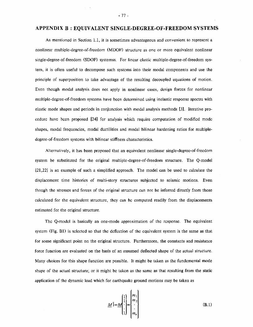
- 77 -

APPENDIX B : EQUIVALENT SINGLE-DEGREE-OF -FREEDOM SYSTEMS

As mentioned in Section 1.1, it is sometimes advantageous and convenient to represent a

nonlinear multiple-degree-of-freedom (MDOF) structure as one or more equivalent nonlinear

single-degree-of-freedom (SDOF) systemss. For linear elastic multiple-degree-of-freedom sys-

tern, it is often useful to decompose such systems into their modal components and use the

principle of superposition to take advantage of the resulting decoupled equations of motion.

Even though modal analysis does not apply in nonlinear cases, design forces for nonlinear

multiple-degree-of-freedom systems have been determined using inelastic response spectra with

elastic mode shapes and periods in conjunction with modal analysis methods [31. Iterative pro-

cedure have been proposed [24] for analysis which require computation of modified mode

shapes, modal frequencies, modal ductilities and modal bilinear hardening ratios for multiple-

degree-of-freedom systems with bilinear stiffness characteristics.

Alternatively, it has been proposed that an equivalent nonlinear single-degree-of-freedom

system be substituted for the original multiple-degree-of-freedom structure. The Q-model

[21,22] is an example of such a simplified approach. The model can be used to calculate the

displacement time histories of multi-story structures subjected to seismic motions. Even

though the stresses and forces of the original structure can not be inferred directly from those

calculated for the equivalent structure, they can be computed readily from the displacements

estimated for the original structure.

The Q-model is basically an one-mode approximation of the response. The equivalent

system (Fig. BD is selected so that the deflection of the equivalent system is the same as that

for some significant point on the original structure. Furthermore, the constants and resistance

force function are evaluated on the basis of an assumed deflected shape of the actual structure.

Many choices for this shape function are possible. It might be taken as the fundemental mode

shape of the actual structure; or it might be taken as the same as that resulting from the static

application of the dynamic load which for earthquake ground motions may be taken as

(B.D

- 78 -

if diagonal mass matrix and unit influence vector are assumed with mi denoting the mass in the

ith degree-of-freedom and n denoting the total number of degree-of-freedoms. However, in

developing the Q-model, it was found [22] advantageous to compute the assumed deflected

shape shape, x, as follows. First, the structure's lateral resistance function is idealized by its

base overturning moment versus roof deflection relationship. This is established by performing

an inelastic analysis of the structure with monotonically increasing lateral forces. The forces are

assumed to have a "triangular" force distribution: the lateral force at a given level is propor-

tional ot the product of the height and mass at that level. Such a base moment-roof displace-

ment curve will be curvilinear in general due to the nonlinearities in the structure. For simpli-

city, the curve may be idealized by two straight lines, the knee of the resulting bilinear relation-

ship implying a synthetic yield point [22], see Fig. B2. The shape function, X, is taken as the

deflected shape when the knee of the bilinear force-displacement curve occurs.

With the shape function calculated as just described, the equivalent mass, damping and

loading can be computed as follow:

M=x'Mx e _

C =x'Cx e _

Fe=-x' Mlug (t)

(B.2)

(B.3)

(B.4)

where Me, Ce and Fe are the effective mass, damping and loading associated with the

equivalent system. The mass and damping matrices of the actual structure and the ground

acceleration are denoted as M, ~ and ug (t) respectively. The resistance of the equivalent

structure can be computed as the modal transformation of the applied lateral forces on the

actual structure and can be written as

R =x'R e (B.5)

where Re is the lateral resistance forces of the equivalent structure and R is the applied lateral

force vector on the actual structure.

With the actual structure represented as just described, the equation of motion becomes

(B.6)

where u is the displacement of the equivalent structure. The displacement of the actual

- 79 -

structure can be obtained by multiplying the assumed deflected shape vector by the solution of

Eqn. B.6. Numerical solution of Eqn. B.6 can be obtained by the computer program described

in this report.

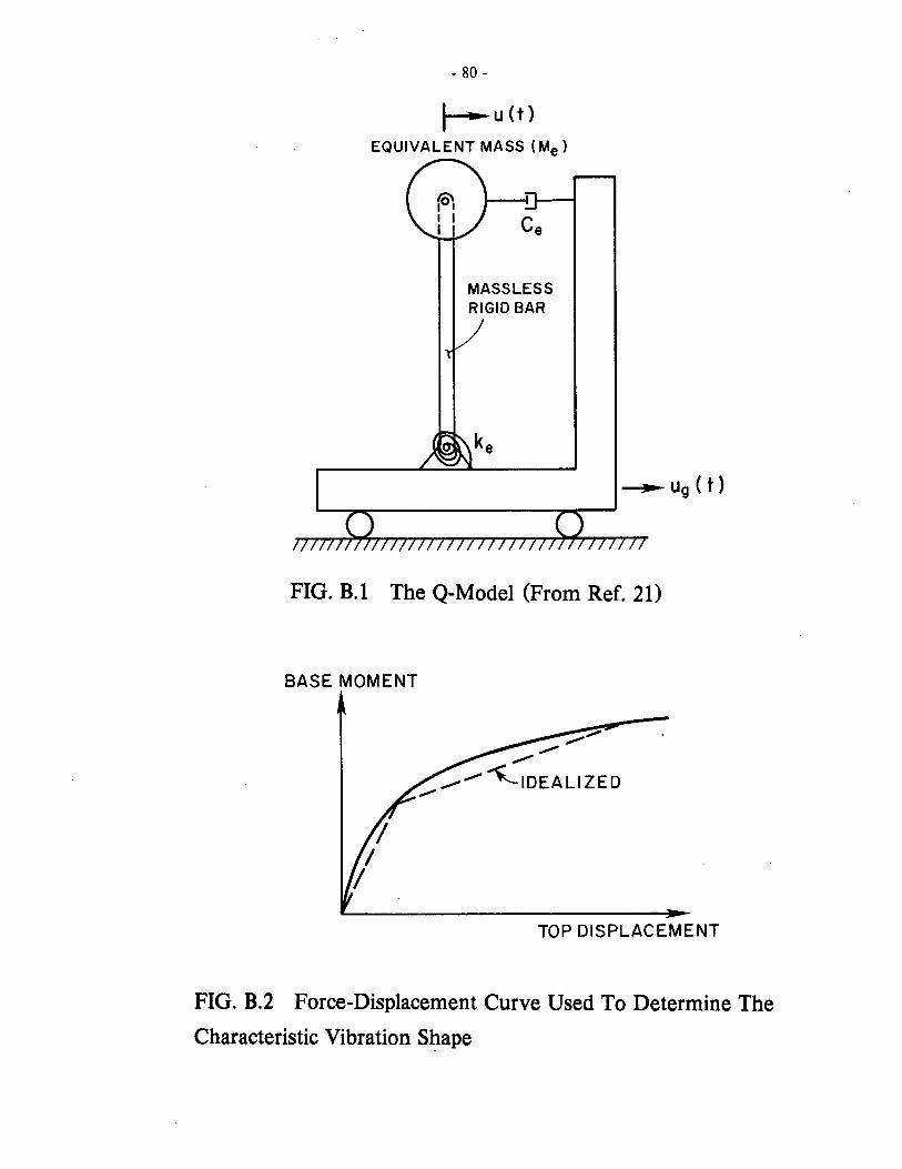
- 80 -

~u{t) EQUIVALENT MASS (Me)

MASSLESS RIGID BAR

FIG. B.l The Q-Model (From Ref. 21)

BASE MOMENT

TOP DISPLACEMENT

FIG. B.2 Force-Displacement Curve Used To Determine The

Characteristic Vibration Shape

-31-

EARTHQUAKE ENGINEERING RESEARCH CENTER REPORTS

NOTE: Numbers in parentheses are Accession Numbers assigned by the National Technical Information Service; these are followed by a price code. Copies of the reports may be ordered from the National Technical Information Service, 5285 Port Royal Road, Springfield, Virginia, 22161. Accession Numbers should be quoted on orders for reports (PB --- ---) and remittance must accompany each order. Reports without this information were not available at time of printing. The complete list of EERC reports (from EERC 67-1) is available upon request from the Earthquake Engineering Research Center, University of California, Berkeley, 47th Street and Hoffman Boulevard, Richmond, California 94804.

UCB/EERC-77/0l "PLUSH - A Computer Program for Probabilistic Finite Element Analysis of Seismic Soil-Structure Inter­action," by M.P. Romo Organista, J. Lysmer and H.B. Seed - 1977 (PB81 177 651)A05

UCB/EERC-77/02 "Soil-Structure Interaction Effects at the Humboldt Bay power Plant in the Ferndale Earthquake of June 7, 1975," by J.E. Valera, H.B. Seed, C.F. Tsai and J. Lysmer - 1977 (PB 265 795)A04

UCB/EERC-77 /03 "Influence of Sample Disturbance on Sand Response to Cyclic Loading," by K. Mori, H. B. Seed and C. K. Chan - 1977 (PB 267 352)A04

UCB/EERC-77/04 "Seismological Studies of Strong Motion Records," by J. Shoja-Taheri - 1977 (PB 269 655)A10

UCB/EERC-77/05 Unassigned

UCB/EERC-77/06 "Developing Methodologies for Evaluating the Earthquake Safety of Existing Buildings," by No.1 -B. Bresler; No.2 - B. Bresler, T. Okada and D. Zisling; No. 3 - T. Okada and B. Bresler; No.4 - V.V. Bertero and B. Bresler - 1977 (PB 267 354)A08

UCB/EERC-77/07 "A Literature Survey - Transverse Strength of Masonry Walls," by Y. Ornote, R.L. Mayes, S.W. Chen and R.W. Clough - 1977 (PB 277 933)A07

UCB/EERC-77/08 "DRAIN-TABS: A Computer Program for Inelastic Earthquake Response of Three Dimensional 8uildings," by R. Guendelman-Israel and G.H. Powell - 1977 (PB 270 693)A07

UC8/EERC-77/09 "SUBWALL: A Special Purpose Finite Element Computer Prograltl for Practical Elastic Analysis and Design of Structural Walls with Substructure Option," by D.Q. Le, H. Peterson and E.P. Popov - 1977 (PB 270 567)A05

UCB/EERC-77/10 "Experimental Evaluation of Seismic Design Methods for Broad Cylindrical Tanks," by D.P. Clough (PB 272 280)A13

UCB/EERC-77/11 "Earthquake Engineering Research at Berkeley -·1976," - 1977 (PB 273 507)A09

UCB/EERC-77/12 "Automated Design of Earthquake Resistant Multistory Steel Building Frames," by N.D. Walker, Jr. - 1977 (PB 276 526)A09

UCB/EERC-77/13 "Concrete Confined by Rectangular Hoops Subjected to Axial Loads," by J. Vallenas, V.V. Bertero and E.P. Popov - 1977 (PB 275 165)A06

UCB/EERC-77/14 "Seismic Strain Induced in the Ground During Earthquakes," by Y. Sugimura - 1977 (PB 284 201);>'04

UCB/EERC-77/15 Unassigned

UCB/EERC-77/16 "Computer Aided Optimum Design of Ductile Reinforced Concrete Moment Resisting Frames," by S.W. Zagajeski and V.V. Bertero - 1977 (PB 280 137)A07

UCB/EERC-77/17 "Earthquake Simulation Testing of a Stepping Frame with Energy-Absorbing Devices," by J.M. Kelly and D.F. Tsztoo - 1977 (PB 273 506)A04

UCB/EERC-77/18 "Inelastic Behavior of Eccentrically Braced Steel Frames under Cyclic Loadings," by C.W. Roeder and E.P. Popov - 1977 (PB 275 526)A15

UCB/EERC-77 /19 "A Simplified Procedure for Estimating Earthquake- Induced Deformations in Dams and Embankments," by F. I. Makdisi and H.B. Seed - 1977 (PB 276 820)A04

UCB/EERC-77/20 "The Performance of Earth Dams during Earthquakes," by H.B. Seed, Folo Makdisi and P. de Alba - 1977 (PB 276 821)A04

UCB/EERC-77/21 "Dynamic Plastic Analysis Using Stress Resultant Finite Element Formulation," by P. Lukkunapvasit and J.M. Kelly - 1977 (PB 275 453)A04

UCB/EERC-77/22 "Preliminary Experimental Study of Seismic Uplift of a Steel Frame," by R.W. Clough and A.A. Huckelbridge 1977 (PB 278 769)A08

UCB/EERC-77/23 "Earthquake Simulator Tests of a Nine-Story Steel Frame with Columns Allowed to Uplift," by A.A. Huckelbridge - 1977 (PB 277 944)A09

UCB/EERC-77/24 "Nonlinear Soil-Structure Interaction of Skew Highway Bridges," by M.-C. Chen and J. Penzien - 1977 (PB 276 176)A07

UCB/EERC-77 /25 "Seismic Analysis of an Offshore Structure Supported on Pile Foundations," by D. D. -N. Liou and J. Penzien 1977 (PB 283 180)A06

UCB/EERC-77/26 "Dynamic Stiffness Matrices for Homogeneous Viscoelastic Half-Planes," by G. Dasgupta and A.K. Chopra -1977 (PB 279 654)A06

-82-

UCB/EERC-77/27 "A Practical Soft Story Earthquake Isolation System," by J.M. Kelly, J.H. Eidinger and C.J. Derham _ 1977 (PB 276 814)A07

UCB/EERC-77/28 "Seismic Safety of Existing Buildings and Incentives for Hazard Mitigation in San Francisco: An Exploratory Study," by A.J. Meltsner - 1977 (PB 281 970)A05

UCB/EERC-77/29 "Dynamic Analysis of Electrohydraulic Shaking Tables," by D. Rea, S. Abedi-Hayati and Y. Takahashi 1977 (PB 282 569)A04

UCB/EERC-77/30 "An Approach for Improving Seismic - Resistant Behavior of Reinforced Concrete Interior Joints," by B. Galunic, V.V. 8ertero and E.P. Popov - 1977 (P8 290 870)A06

UC8/EERC-78/01 "The Development of Energy-Absorbing Devices for Aseismic 8ase Isolation Systems," by J .~1. Kelly and D.F. Tsztoo - 1978 (PB 284 978)A04

UCB/EERC-78/02 "Effect of Tensile Prestrain on the Cyclic Response of Structural Steel Connections, by J.S. Bouwkamp and A. Mukhopadhyay - 1978

UCB/EERC-78/03 "Experimental Results of an Earthquake Isolation System using Natural Rubber Bearings," by J.M. Eidinger and J.M. Kelly - 1978 (PE 281 686)A04

UCB/EERC-78/04 "Seismic Behavior of Tall Liquid Storage Tanks," by A. Niwa - 1978 (PE 284 017)A14

UCB/EERC-78/05 "Hysteretic Behavior of Reinforced Concrete Columns Subjected to High Axial and Cyclic Shear Forces," by S.W. Zagajeski, V.V. Bertero and J.G. Bouwkamp - 1978 (PB 283 858)A13

UCB/EERC-78/06 "Three Dimensional Inelastic Frame Elements for the .;NSR-I Program," by.;. Riahi, D.G. Rowand G.H. Powell - 1978 (P8 295 755)A04

UCB/EERC-78/07 "Studies of Structural Response to Earthquake Ground Motion," by O.A. Lopez and A.K. Chopra - 1978 (P8 282 790)A05

UC8/EERC-78/08 ".". Laboratory Study of the Fluid-Structure Interaction of Submerged Tanks and Caissons in Earthquakes," by R.C. Byrd - 1978 (P8 284 957)A08

UCB/EERC-78/09 Unassigned

UCB/EERC-78/10 "Seismic Performance of Nonstructural and Secondary Structural Elements," by I. Sakamoto - 1978 (PB8l 154 593)A05

UCB/EERC-78/11

UCB/EERC-7B/12

UCB/EERC-78/13

UCB/EERC-78/l4

UCB/EERC-78/15

UCB/EERC-78/16

UCB/EERC-78/17

UCB/EERC-78/18

UCB!EERC-78/19

UCB/EERC-78/20

UCB/EERC-78/21

UCB/EERC-78/22

UCB/EERC-78/23

UCB/EERC-78/24

UCB/EERC-78/25

"Mathematical 110delling of Hysteresis Loops for Reinforced Concrete Columns," by S. Nakata, T. S£,roul and J. Penzien - 1978 (PB 298 274)A05

"Damageability in Existing 8uildings," by T. 8lejwas and B. Bresler - 1978 (PB 80 166 978)A05

"Dynamic Behavior of a Pedestal Base Multistory Building," by R.M. Stephen, E.L. Wilson, J.G. Bouwkamp and M. Button - 1978 (PB 286 650)A08

"Seismic Response of Bridges - Case Studies," by R.A. Imbsen, V. Nutt and J. Penzien - 1978 (PB 286 503)AIO

"A Substructure Technique for Nonlinear Static and Dynamic Analysis," by D.G. Rowand S.H. Powell -1978 (PB 288 077)AIO

"Seismic Risk Studies for San Francisco and for the Greater San Francisco Bay Area," by C.S. Oliveira -1978 (PB 81 120 115)A07

"Strength of Timber Roof Connections Subjected to Cyclic Loads," by P. Gulkan, R.L. Mayes and R.W. Clough - 1978 (HUD-OOO l49l)A07

"Response of K-Braced Steel Frame Models to Lateral Loads," by J.G. Bouwkamp, R.M. Stephen and E.P. Popov - 1978

"Rational Design Methods for Light Equipment in Structures Subjected to Ground Motion," by J.L. Sackman and J.M. Kelly - 1978 (P8 292 357)A04

"Testing of a Wind Restraint for Aseismic Base Isolation," by J.M. Kelly and D.E. Chitty - 1978 (PB 292 833) AD3

"APOLLO - A Computer Program for the Analysis of Pore Pressure Generation and Dissipation in Horizontal Sand Layers During Cyclic or Earthquake Loading," by P.P. Martin and H.B. Seed - 1978 (FB 292 835)A04

"Optimal Design of an Earthquake Isolation System," by M.A. 8hatti, K.S. Pister and E. Polak - 1978 (P8 294 73S)AD6

"MASH - A Computer Program for the Non-Linear Analysis of Vertically Propagating Shear Waves in Horizontally Layered Deposits," by P.P. Martin and H.B. Seed - 1978 (PB 293 101)A05

"Investigation of the Elastic Characteristics of a Three Story Steel Frame Using System Identification," by I. Kaya and H.D. McNiven - 1978 (PB 296 225)A06

"Investigation of the Nonlinear Characteristics of a Three-Story Steel Frame Using System Identification," by 1. Kaya and H.D. McNiven - 1978 (PB 301 363)AOS

-83-

UCB/EERC-78/26 "Studies of Strong Ground Motion in Taiwan," by Y.M. Hsiung, B.A. Bolt and J. Penzien - 1978 (PB 298 436)A06

llCB/EERC-78/27 "Cyclic Loading Tests of l1asonry Single Piers: volume 1 - Height to width Ratio of 2," by P .A. Hidalgo, R.L. 11ayes, H.D. McNiven and R.'.v. Clough - 1978 (PB 296 211)A07

UC3/EERC-78/28 "Cyclic Loading Tests of Masonry Single Piers: volume 2 - Height to width Ratio of 1." by S.-W.J. C:'en, P.A. Hidalgo, R.L. Mayes, R.W. Clough and H.D. McNiven - 1978 (PB 296 212)A09

UCB/EERC-78129 ";"nalytical Procedures in Soil Dynamics," by J. Lysmer - 1978 (PB 298 445)';06

UCB/EERC-79/01 "Hysteretic Behavior of Lightweight Reinforced Concrete Beam-Column Subassemblages." by B. f"orzani, E.P. Popov and V.V. Bertero - il.pdl 1979(PB 298 267)A06

UCB/EERC-79/02 "The Development of a Mathematical M:ldel to Predict the Flexural Response of Reinforced Concrete Beams to Cyclic Loads, Using System Identification," by J. Stanton & H. McNiven - Jan. 1979(PB 295 875)AlO

UCB/EERC-79/03 "Linear and Nonlinear Earthquake Response of Simple Torsionally Coupled Systems," by C.L. Kan and A.K. Chopra - Feb. 1979(PB 29B 262)A06

UCB/EERC-79/04 "'; ~lathematical ~bdel 0 f Masonry for Predicting its Linear Seismic Response Characteristi::s," by Y. Mengi and H.D. McNiven - Feb. 1979(PB 29B 266) A06

uCB/EERC-79/05 "Mechanical Behavior of Lightweight Concrete Confined by Different Types of Lateral Reinforcement," by M.A. Manrique, V.V. Bertero and E.P. Popov - May 1979(PB 301 114)A06

uCB/EERC-79/06 '''Static Tilt Tests of a Tall Cylindrical Liquid Storage Tank," by R.W. Clough and A. Niwa - Feb. 1979 (PB 301 167)A06

UCB/EERC-79/07 "The Design of Steel Energy Absorbing Restrainers and Their Incorporation into Nuclear Power Plants for Enhanced Safety: Volume 1 - Summary Report," by P.N. Spencer, V.F. Zackay, and E.R. Parker -Feb. 1979(UCB/EERC-79/07)A09

UCBjEERC-79/08 "The Design of Steel Energy Absorbing Restrainers and Their Incorporation into Nuclear Power Plants for Enhanced Safety: Volume 2 - The Development of Analyses for Reactor System Piping, ""Simple Systems" by M.C. Lee, J. Penzien, A.K. Chopra and K, Suzuki "Complex Systems" by G.H. Powell, E.L. Wilson, R.W. Clough and D.G. Row - Feb. 1979(UCB/EERC-79/08)AIO

lJCB/EERC-79/09 "The Design of Steel Energy Absorbing Restrainers and Their Incorporation into Nuclear PONer Plants for Enhanced Safety: Volume 3-Evaluation of Commercial Steels," by W.S. OWen, R.~1.N. Pelloux, R.O. Ritchie, M. Faral, T. Ohhashi, J. Toplosky, S.J. Hartman, V.F. Zackay and E.R. Parker -Feb. 1979(UCB/EERC-79/09)A04

UCB/EERC-79/10 "The Design of Steel Energy Absorbing Restrainers and Their Incorporation into Nuclear Power Plants for Enl-,anced Safety: Volume 4 - A Review of Energy-Absorbing I;Jevices," by J. ~l. Kelly and M.S. Skinner - Feb. 1979(UCB/EERC-79/10)A04

UCB/EERC-79/ll "Conservatism In Summation Rules for Closely Spaced Modes," by J.M. Kelly and J.L. Sackman - Hay 1979(PB 301 328)A03

UCB/EERC-79/12 "Cyclic Loading Tests of Masonry Single Piers; Volume 3 - Height to Width Ratio of 0.5," by P.A. Hidalgo, R.L. Mayes, H.D. McNiven and R.W. Clough - May 1979(PB 301 321)AOB

UCB/EERC- 79/13 "Cyclic Behavior 0 f Dense Course-Grained Materials in Relation to the Seismic Stability of Darns," by N.G. Banerjee, H.B. Seed and C.K. Chan - June 1979(PB 301 373)A13

UCB/EERC-79/14 "Seismic Behavior of Reinforced Concrete Interior Beam-Column Subassemblages," by S. Viwathanatepa, E.P. Popcv and V.V. Bertero - June 1979(PB 301 326)AlO

UCB/EERC-79/15 "Optimal Design of Localized Nonlinear Systems with Dual Performance Criteria Under Earthquake Excitations," by M.A. Bhatti - July 1979(PB BO 167 109)A06

UCB/EERC-79/16 "OPTDYN - A General Purpose Optimization Proqram for Problems with or wi thout Dynamic Cons traints," by M.A. Bhatti, E. Polak and K.S. Pister - July 1979(PB 80 167 091)A05

UCB/EERC-79/17 "ANSR-II, Analysis of Nonlinear Structural Response, Users Manual," by D.P. t~ondkar and G.H. Powell July 1979 (PB 80 113 301) A05

UCB/EERC-79/1B "Soil Structure Interaction in Different Seismic Environments," A. G:>mez-Masso, J. Lysmer, J .-C. Chen and H.B. Seed - August 1979(PB 80 101 520)A04

UCB/EERC-79/19 "AR1~A M:ldels for Earthquake Ground Motions," by M.K. Chang, J.W. Kwiatkowski, R.F. Nau, R.M. Oliver and K.S. Pister - July 1979(PB 301 166)A05

UCB/EERC-79/20 "Hysteretic Behavior of Reinforced Concrete Structural Walls," by J. M. Vallenas, V. V. Bertero and E.P. Popov - August 1979(PB 80 165 905)Al2

UCB/EERC-79/21 "Studies on High-Frequency Vibrations of Buildings - 1: lhe Column Effect," by J. Lubliner - August1979 (PB BO 158 553)A03

UCB/EERC-79/22 "Effects of Generalized Loadings on Bond Reinforcing Bars Embedded in Confined Concrete Blocks," by S. Viwathanatepa, E.P. Popov and V.V. Bertero - August 1979(PB 81 124 018)A14

UCB/EERC- 79/23 "Shaking Table Study of Single-Story Masonry Houses, Volume 1 : Test Structures 1 and 2, " by P. Gi.i1.kan, R.L. Mayes and R.W. Clough - Sep1L 1979 (HUD-OOO 1763)A12

UCB/EERC-79/24 "Shaking Table Study of Single-Story Masonry Houses, Volume 2 : Test Structures 3 and 4, " by P. Gulkan, R.L. Mayes and R.W. Clough - Sept. 1979 (HUD-OOO 1836)A12

UCB/EERC-79/25 "Shaking Table Study of Single-Story Masonry Houses, Volume 3: Summary, Conclusions and Recommendations," by R.W. Clough, R.L. Mayes and P. Gulkan - Sept. 1979 (HUO-OOO 1837)A06

-04-

UCB/EERC-79/26 "Recommendations tor a U.S.-Japan Cooperative Research Program Utilizing Large-Scale Testing Facilities," by U.S.-Japan Planning Group - Sept. 1979(PB 301 407)A06

UCB/SERC-,9/27 "Earthquake-Induced Liquefaction Near Lake Amatitlan, Guatemala," by H.B. Seed, I. Arango, C.K. 01 an , A. Gomez-Masso and R. Grant de Ascoli - Sept. 1979(NUREG-CRl34l)A03

UCB/EERC-79/28 "Infill Panels: ,Their Influence on Seismic Response of Buildings," by J.W. Axley and V.V. 8ertero Sept. 1979(PB 80 163 37l)AlO

UCB/EERC-79/29 "3D Truss Bar Element (Type 1) for the ANSR-II Program," by D.P. Mondkar and G.H. Powell - Nov. 1979 (PB 80 169 709)A02

UCS/EERC-79/30 "20 Beam-Coltunn Element (Type 5 - Parallel Element Theory) for the ANSR-II Program," by D.G. Row, G.H. Powell and D.P. Mondkar - Dec. 1979(PB 80 167 224)A03

UCB/EERC-79/31 "3D Beam-Column Element (Type 2 - Parallel Element Theory) for the ANSR-II Program," by A. Rial''lL G.H. Powell and D.P. Mondkar - Dec. 1979(PB SO 167 216)A03

UCB/EERC-79/32 "On Response of Structures to Stationarj Excitation," by A. Der Kiureghian - Dec. 1979(PS S0166 929) ~.o3

UCS/EERC-79/33 "Undisturbed Sampling and Cyclic Load Testing of Sands," by S. Singh, H.B. Seed and C.K. Chan Dec. 1979(ADA 087 29S)A07

VCB/EERC-79/34 "Interaction Effects of Simultaneous Torsional and Compressional Cyclic Loading of Sand," by P.M. Griffin and W.N. Houston - Dec. 1979(ADA 092 352)A15

VCB/EERC-SO/Ol "Earthquake Response of Concrete Gravity Dams Including Hydrodynamic and Foundation Interaction Effects," by A.K. Chopra, P. Chakrabarti and S. Gupta - Jan. 1980(AD-A087297)AlO

UCS/EERC-80/02 "Rocking Response of Rigid Blocks to Earthquakes," by C.S. Yim, A.K. Chopra and J. Per.zien - Jan. 1980 (PBBO 166 002)A04

eCB/EERC-30/03 "Optimum Inelastic Design of Seismic-Resistant Reinforced Concrete Frame Structures," by S. 'II. Zagaj eski and V.V. Bertero - Jan. 1980(PB80 164 635)A06

UCB/EERC-80/04 "Effects of Amount and Arrangement of Wall-Panel Reinforcement on Hysteretic Behavior of Peinforced concrete 'rlalls," by R. Iliya and 'J. V. Be,rtero - Feb. 1980 (P881 122 525) A09

DCS/EERC-BO/OS "Shaking Table Research on Concrete Dam Models," by .~. Niwa and R.W. Clough - Sept. 1980(PBSl122 368);'00

DCB/EERC-80/00 "The Design of Steel Energy-Absorbing Restrainers and ':heir Incorporation into Nuclear Power Plants for Enhanced Safety (Vol lAJ: Piping with Energy Absorbing Restrainers: Parameter Study on Small Systems," by G.H. Powell, C. Oughourlian and J. Simons - June 1980

VCE/EERC-sO/07 "Inelastic Torsional Response of Structures Subjected to Earthquake Ground 110tions," by Y. Yamazaki April 19s0(PBsl 122 327)AOs

UCB/EERe-80/0s "Study of X-Sraced Steel Frame Structures Under Earthquake S,imulation," by Y. Ghanaat - April 1980 (PB8l 122 335)All

UCB/EERC-BO/09 "Hybrid 110delling of Soil-Structure Interaction," by S. Gupta, T.W. Lin, J. ?enzien and C.S. Yeh 1-lay 1980 (PB8l 122 319) .'.07

UCB/EERC-BO/lO "General Applicability of a Nonlinear Model of a One Story Steel Frame," by B. 1. Sveinsson and H.D. ~cNiven - Hay 1980(PB8l 124 877)A06

UCB/EERC-80/11 "A Green-Function Method for Wave Interaction 'Nith a Submerged Body," by W. Kioka - April 1980 (PBSl 122 269)1'.07

DCB/EERC-SO/12 "Hydrodynamic Pressure and Added ~lass for .'u<isymmetric Bodies," by F. Nilrat - May 1980 (PBSl 122 343) AGS

UCB/EERC-BO/13 "Treatment of Non-Linear Drag Forces Acting on Offshore Platforms," by B. V'. Dao and J. Penzien May 1980(PB8l 153 413)A07

VCB/EERC-80/l4 "20 Plane/.'u<isymmetric Solid Element (Type 3 - Elastic or Elastic-Perfectly Plastic) for the ANSR-II program," by D.P. Mondkar and G.H. Powell - July 1980(PB8l 122 350)A03

UCB/EERC-BO/15 "A Response Spectrum Method for Random Vibrations," by A. Der Kiureghian - June 1980 (PB8ll22 301) A03

DCS/EERC-SO/16 "Cyclic Inelastic Buckling of TUbular Steel Braces," by V.A. Zayas, E.P. Popov and S.A. ,·lahin June 1980(PB8l 124 885)A10

VCB/EERC-SO/l7 "Dynamic Response of Simple Arch Dams Including Hydrodynamic Interaction," by C. S. Pon:er and A.K. Chopra - July 1980(PB8l 124 000)A13

UCB/EERC-80/l8 "Experimental Testing of a Friction Damped Aseismic Base Isolation System with Fail-Safe Characteristics," by J.M. Kelly, K.E. Beucke and M.S. Skinner - July 1980(pS8l 148 595)A04

UCB!EERC-80/l9 "The Design of Steel Energy-Absorbing Restrainers and their Incorporation into Nuclear Power Plants for Enhanced Safety (Vol lB): Stochastic Seismic Analyses of Nuclear Power Plant Structures and Piping Systems Subjected to Multiple SUPDort Excitations," by M.C. Lee and J. Penzien - June 1980

UCB/EERC-BO/20 "The Design of Steel Energy-Absorbing Restrainers and their Incorporation into Nuclear Power Plants for Enhanced Safety (vol lC): Numerical 11ethod for Dynamic Substructure Analysis," by J. M. Dickens and E.L. Wilson - June 1980

UCB/EERC-SO/2l "The Design of Steel Energy-Absorbing Restrainers and their Incorporation into Nuclear Power Plants for Enhanced Safety (Vol 2): Development and Testing of Restraints for Nuclear Piping Systems," by J.M. Kelly and M.S. Skinner - June 1980

UCS/EERC-80/22 "3D Solid Element (Type 4-Elastic or Elastic-perfectly-Plastic) for the ANSR-II Program," by D.P. Mondkar and G.H. Powell - July 1980(PBSl 123 242)A03

UCE/EERC-80/23 "Gap-Friction Element (Type 5) for the ANSR-II Program," by D.P. Mondkar and G.H. Powell - July 1980 (PBSl 122 285)A03

-85-

UCB/EERC-80/24 "U-Bar Restraint Element (Type 11) for the ANSR-II Program," by C. Oughourlian and G.H. Powell July 1980(P881 122 293)A03

UCB/EERC-80/25 "Testing of a Natural Rubber Base Isolation System by an Explosively Simulated Earthquake," by J.H. Kelly - August 1980(PB81 201 360)A04

UCB/EERC-30/26 "Input Identification from Structural Vibrational Response," by Y. Hu - August 1980(PB81 152 308)AOS

UCB/EERC-80/27 "Cyclic Inelastic Behavior of Steel Offshore Structures," bv V. A. Zayas, S. A. ~Iahin and E. P. Popov August 1980(PB81 196 180lA1S •

UCB/EERC-80/28 "Shaking Table Testing of a Reinforced Concrete Frame '''ith Biaxial Response," by M.G. Oliva October 1980(PB81 154 304)AIO

UCB/EERC-80/29 "Dynamic Properties of a 'r'"elve-Story Prefabricated Panel Building," by J.G. Bouwkamp, J.P. Kollegger and R.M. Stephen - October 1980(PB82 117 l28lA06

UCB/EERC-80130 "Dynamic Properties of an Eight-Story Prefabricated Panel Building," by J.G. Bouwkamp, J.P. Kollegger and R.M. Stephen - October 1980(PB8l 200 313)A05

eCB/EERC-80/31 "Predictive Dynamic Response of Panel Type Structures Under Earthquakes," by ';.P. Kollegger and J.G. Bouwkamp - October 1980(PB81 152 3l6)A04

UCB/EERC-80/32 "The Design of Steel Energy-.~sorbing Restrainers and their Incorporation into Nuclear Power Plants for Enhanced Safety (Vol 3): Testing of ':ommercial Steels in Low-Cycle Torsional Fatique," by P. =~~~~~r, E.R. Parker, E. Jongewaard and M. Crary

ULB/EEhC-80/33 "The Jeslgn of Steel Energy-Absorbing Restrainers and their Incorporation into Nuclear Po .... er Plants for Enhanced Safety (Vol 4): Shaking Table Tests of Piping System~ with Energy-Absorbing Restrainers," by S.F. Stiemer and W.G. Godden - Sept. 1980

UCB/!':ERC-30/34 "':'he Design of Steel Energy-Absorbing Restrainers "nd their Incorpur"tion into Nuclear Power Plants for Enh"nced Safety (Vol 5): Summary Report," by P. Spencer

UCJ/EERC-80/35 "Experimental Testing of an Energy-,~sorbing Base Isolation System," by J.~.1. Kelly, >1.S. Skinner and K.E. Beucke - October 1980(PB8l lS4 072)A04

UC3/EERC-30/36 "Simulating and Analyzing Artificial ~lon-Stationary Earthquake Ground ~lotions," by R.F. Nau, R.)-1. Oliver and K.S. Pister - October 1980(PB8l 153 397)A04

UC3/EERC-80/37 "Earthquake Engineering at Berkeley - 1980," - Sept. 1980(P381 20S 374)A09

UCS/EERC-80/38 "Inelastic Seismic ,'u1alysis of Large Panel Buildings," by V. Schricker and G.H. Powell - Sept. 1980 (PB8l 154 338)A13

UCB/EERC-80/39 "Dynamic Response of Embankment, Concrete-Gr"vity and ".rch Dams Including Hydrodynamic Interaction," by J.F. Hall and A.K. Chopra - October 1980(PB81 lS2 324)All

UCB/EERC-BO/40 "Inelastic Buckling of Steel Str'lts Under Cyclic Load Reversal_," by R.G. Black, W.A. Wenger and E.P. Popov - Octo~er 1980(PB8l 154 312)A08

UCB/EERC-SO/4l "Influence of Site Characteristics on Building Damage During the October 3, 1974 Lima Earthquake," by P. Repetto, I. Arango and H.B. Seed - Sept. 1980(PBBl 161 739)A05 .

lJC3/EERC-80/42 "Evalu"tion of a Shaking Table Test Program on Response Behavior of a 'r'No Story Reinforced Concrete Frame," by J.M. Blondet, R.W. Clough and S.A. /·lahin

TJCB/E,ERC-8C/43 "r~odelling of Soil-Structure Interaction by Finite and Infinite Elements," by F. ~'ledina -December 1980(PB81 229 270)A04

UCB/EERC-8l/01 "Control of Seismic Response of Piping Systems and Other Structures by Base Isolation," edited by J.:1. Kelly - January 1981 (PB8l 200 73S)A05

UCB/EERC-81/02 "OPTNSR - An Interactive Software System for Optimal Design of Statically and Dynamically Loaded Structures with Nonlinear Response," by M.A. Bhatti, V. Ciampi and K.S. Pister - January 1981 (PB8l 218 851)A09

UCB/EERC-8l/03 "Analysis of Local Variations in Free Field Seismic Ground Motions," by J.-C. Chen, J. Lysmer and H.B. Seed - January 1981 (AD-AC99508)A13

UCB/EERC-81/04 "Inelastic Structural Modeling of Braced Offshore Platforms for Seismic Loading," by V.A. Zayas, P.-S.B. Shing, S.A. Mahin and E.P. Popov - January 1981(PB82 138 777)A07

UCB/EERC-81/0S "Dynamic Response of Light Equipment in Structures," by A. Der Kiureghian, J.L. Sackman and B. Nour­Omid - April 1981 (PB81 218 497)A04

UCB/EERC-8l/06 "Preliminary Experimental Investigation of a Broad Base Liquid Storage Tank," by J.G. Bouwkamp, J.P. Kollegger and R.M. Stephen - May 1981(PB82 140 38S)A03

UCB/EERC-BI/07 "The Seismic Resistant Design of Reinforced Concrete Coupled Structural Walls," by A.E. Aktan and V.V. Bertero - June 1981(PB82 113 358)All

UCB/EERC-81/08 "The Undrained Shearing Resistance of Cohesive Soils at Large Deformations," by M.R. Pyles and H.B. Seed - August 1981

UCB/EERC-81/09 "Experimental Behavior of a Spatial Piping System with Steel Energy .;bsorbers Subjected to a Simulated Differential Seismic Input," by S.F. Stiemer, W.G. Godden and J.M. Kelly - July 1981

-86-

UCB/EERC-81/l0 "Evaluation of Seismic Design Provisions for Masonry in the United States," by B.I. sveinsson, R.L. Mayes and H.O. McNiven - August 1981 (PB82 166 075)A08

UCB/EERC-8l/l1 "Two-Dimensional Hybrid Modelling of Soil-Structure Interaction," by T.-J. Tzong, S. Gupta and J. Penzien - August 1981(PB82 142 118)A04

UCB/EERC-8l/l2 "Studies on Effects of Infills in Seismic Resistant RIC Construction," by S. Brakken and V.V. Bertero -September 1981 (PB82 166 190)A09

UCB/EERC-8l/l3 "Linear Models to Predict the Iionlinear Seismic Behavior of a One-Story Steel Frame," by H. Valdimarsson, A.H. Shah and H.O. McNiven - September 1981(PB82 138 793)A07

UCB/EERC-81/14 "TLUsH: A Computer Program for the Three-Dimensional Cynamic Analysis of Earth Cams," by T. Kagawa, L.H. MeJia, H.B. Seed and J. Lysmer - September 1981(PB82 139 940)A06

UCB/EERC-Bl/lS "Three Cimensional Cynamic Response Analysis of Earth Cams," by L.H. Mejia and H.B. Seed - September 1981 (PB82 137 274)A12

UCB/EERC-81/16 "Experimental Study of Lead and Elastomeric Campers for Base Isolation Systems," by J.M. Kelly and s.B. Hodder - October 1981 (PB82 166 IB2)A05

UCB/EERC-81/17 "The Influence of Base Isolation on the Seismic Response of Light Secondary Equipment," by J.M. Kelly -April 1981 (PB82 255 266)A04

UCB/EERC-8l/18 "Studies on Evaluation of Shaking Table Response Analysis Procedures," by J. Marcial Blondet - November 1981 (PB82 197 278)AlO

UCB/EERC-8l/l9 "CELIGHT.STRUCT: A Computer-Aided Design Environment for Structural Engineering," by R.J. Balling, K.S. Pister and E. Polak - December 1981 (PB82 218 496)A07

UCB/EERC-81/20 "Optimal Design of Seismic-Resistant Planar Steel Frames," by R.J. Balling, V. Ciampi, K.S. Pister and E. Polak - Cecember 1981 (PB82 220 l79)A07

UCB/EERC-82/0l "Dynamic Behavior of Ground for Seismic Analysis of Lifeline Systems," by T. Sate and A. Der Kiureghian -January 1982 (PB82 218 926)A05

UCB/EERC-82/02 "Shaking Table Tests of a Tubular steel Frame Model," by Y. Ghanaat and R. W. Clough - January 1982 (PB82 220 l6l)A07

UCB/EERC-82/03 "Behavior of a piping System under Seismic Excitation: Experimental Investigations of a Spatial Piping system supported by Mechanical Shock Arrestors and Steel Energy Absorbing Devices under Seismic Excitation," by S. schneider, H.-H. Lee and W. G. Godden - May 1982 (PBB3 172 544)A09

UCB/EERC-82/04 "New Approaches for the Dynamic Analysis of Large Structural systems," by E. L. Wilson - June 1982 (PB83 148 080)A05

UCB/EERC-82/05 "Model Study of Effects of Damage on the Vibration Properties of Steel Offshore Platforms," by F. Shahrivar and J. G. Bouwkamp - June- 1982 (PB83 148 742)AlO

UCB/EERC-82/06 "States of the Art and Practice in the Optimum seismic Design and Analytical Response Prediction of RIC Frame-Wall Structures," by A. E. Aktan and V. V. Bertero - July 1982 (PB83 147 736)A05

UCB/EERC-82/07 "Further Study of the Earthquake Response of a Broad Cylindrical Liquid-Storage Tank Model," by G. C. Manos and R. W. Clough - July 1982 (PB83 147 744)All

UCB/EERC-82/08 "An Evaluation of the Design and Analytical Seismic Response of a Seven Story Reinforced Concrete Frame - Wall Structure," by F. A. Charney and V. V. Bertero - July 1982(PB83 157 628)A09

UCB/EERC-82/09 "Fluid-Structure Interactions: Added Mass Computations for Incompressible Fluid." by J. S.-H. Kuo -August 1982 (PB83 156 281)A07

UCB/EERC-82/10 "Joint-opening Nonlinear Mechanism: Interface Smeared Crack Hodel," by J. S.-H. Kuo -August 1982 (PB83 149 19S)A05

UCB/EERC-82/11 "Cynamic Response Analysis of Techi Dam," by R. W. Clough, R. H. Stephen and J. S.-H. Kuo -August 1982 (PB83 147 496)A06

UCB/EERC-82/12 "Prediction of the Seismic Responses of RIC Frame-Coupled Wall Structures," by A. E. Aktan, V. V. Bertero and M. Piazza - August 1982 (PB83 149 203~09

UCB/EERC-82/l3 "Preliminary Report on the SMART 1 Strong Motion Array in Taiwan," by B. A. Bolt, C. H. Loh, J. Penzien, Y. B. Tsai and Y. T. Yeh - August 1982 (PB83 159 400)AlO

UCB/EERC-82/14 "Shaking-Table Studies of an Eccentrically X-Braced Steel Structure," by M. S. Yang - September 1982 (PBS3 260 778)Al2

UCB/EERC-S2/1S "The Performance of Stairways in Earthquakes," by C. Reba, J. W. Axley and V. V. Bertero - September 1982 (PB83 157 693)A07

UCB/EERC-82/16 "The Behavior of Submerged Multiple Bodies in Earthquakes," by W.-G. Liao - Sept. 1982 (PB83 158 709)A07

UCB/EERC-82/17 "Effects of Concrete Types and Loading Conditions on Local Bond-Slip Relationships," by A. C. Cowell, E. P. Popov and V. V. Bertero - September 1982 (PBS3 153 577)A04

UCB/EERC-82/l8

UCB/EERC-82/l9

UCB/EERC-82/20

UCB/EERC-82/21

UCB/EERC-82/22

UCB/EERC-82/23

UCB/EERC-82/24

UCB/EERC-82/25

UCB/EERC-82/26

UCB/EERC-82/27

UCB/EERC-83/0l

UCB/EERC-83/02

UCB/EERC-83/03

UCB/EERC-83/04

UCB/EERC-83/05

UCB/EERC-83/06

UCB/EERC-83/07

UCB/EERC-83/0R

UCB/EERC-83/09

UCB/EERC-83/l0

UCB/EERC-83/11

UCB/EERC-83/l2

UCB/EERC-83/l3

UCB/EERC-83/l4

UCB/EERC-83/l5

UCB/EERC-83/l6

UCB/EERC-83/l7

-87-

"Mechanical Behavior of Shear Wall Vertical Boundary Members: An Experimental Investigation," by M. T. Wagner and V. V. Bertero - October 1982 (PB83 159 764)A05

"Experimental Studies of Multi-support Seismic Loading on Piping Systems," by J. M. Kelly and A. D. Cowell - November 1982

"Generalized Plastic Hinge Concepts for 3D Beam-Column Elements," by P. F.-S. Chen and G. H. Powell -November 1982 (PB03 217 ~81)Al3

"ANSR-III: General Purpose Computer Program for Nonlinear Structural Analysis," by C. V. Oughourlian and G. H. Powell - November 1982 (PB83 251 330)A12

"Solution Strategies for Statically Loaded Nonlinear Structures," by J. W. Simons and G. H. Powell -November 1982 (PB83 197 970)A06

"Analytical Model of Deformed Bar Anchorages under Generalized Excitations," by V. Ciampi, R. Eligehausen, V. V. Bertero and E. P. Popov - November 1982 (PB83 169 532)A06

"A Mathematical Model for the Response of Masonry Walls to Dynamic Excitations," by H. Sucuoglu, Y. Mengi and H. D. McNiven - November 1982 (PB83 169 011)A07

"Earth~uake Response Considerations of Broad Liquid Storage Tanks," by F. J. Cambra - November 1982 (PB83 ~Sl 21S)A09

"Computational Models for Cyclic Plasticity, Rate Dependence and Creep," by B. Mosaddad and G. H. Powell - November 1982 (PB83 245 829)A08

"Inelastic Analysis of Piping and Tubular Structures," by M. Mahasuverachai and G. H. Powell - November 1982 .(PB83 249 .987)A07

"The Economic Feasibility of Seismic Rehabilitation of Buildings by Base Isolation," by J. M. Kelly -January 1983 (pB83 197 988)A05

"Seismic Moment Connections for Moment-Resisting Steel Frames," by E. P. Popov - January 1983 (PB83 195 U2)A04

"Design of Links and Beam-to-Co1umn Connections for Eccentrically Braced Steel Frames," by E. P. Popov and J. O. Malley - January 1983 (pB83 194 811)A04

"Numerical Techniques for the Evaluation of Soil-structure Interaction Effects in the Time Domain," by E. Bayo and E. L. Wilson - February 1983 (PB83 24S 60S)A09

"A Transducer for Measuring the Internal Forces in the ColUmns of a Frame-Wall Reinforced Concrete Structure," by R. Sause and V. V. Bertero - May 1983 (pB84 ~9 494)A06

"Dynamic Interactions between Floating Ice and Offshore structures," by P. Croteau - May 1983 (1'B84 ~9 486l.Al6

"Dynamic Analysis of Multiply Tuned and Arbitrarily Supported Secondary Systems," by T. 19usa and A. Der Kiureghian - June 1983 (pB84 U8 2721All

"A Laboratory Study of Submerged Multi-body systems in Earthquakes," by G. R. Ansari - June 1983 (PB83 261 842)Al7

"Effects of Transient Foundation Uplift on Earthquake Response of Structures," by C.-S. Vim and A. K. Chopra - June 1983 (PB83 261 396)A07

"Optimal Design of Friction-Braced Frames under Seismic Loading," by M, A. Austin and K, S. Pister -June 1983 (PB84 119 288,A06

"Shaking Table Study of Single-Story Masonry Houses: Dynamic Performance under Three Component Seismic Input and Recommendations," by G. C. Manos, R. W. Clough and R. L. Mayes - June 1983

"Experimental Error Propagation in pseudodynamic Testing," by P. B. Shing and S. A. Mahin - June 1983 (PB84 119 270)A09

"Experimental and Analytical Predictions of the Mechanical Characteristics of a LIS-scale Model of a 7-story RIC Frame-Wall Building Structure," by A. E. Aktan, V. V. Bertero, A. A. Chowdhury and T. Nagashima - August 1983 (pB84 119 2l3)A07

"Shaking Table Tests of Large-panel Precast Concrete Building System Assemblages," by ~I. G. Oliva and R. w. Clough - August 1983

"Seismic Behavior of Active Beam Links in Eccentrically Braced Frames," by K. D. Hjelmstad and E. P. Popov - July 1983 (PB84 119 6761A09

"System Identification of Structures with Joint Rotation," by J. S. Dimsdale and H. D. McNiven -July 1983

"Construction of Inelastic Response Spectra for Single-Degree-of-Freedom Systems," by S. Mahin and J. Lin - July 1983