Constructing the Decision Model

Y. İlker TOPCU, Ph.D.

www.ilkertopcu.net www.ilkertopcu.org www.ilkertopcu.info

www.facebook.com/yitopcu

twitter.com/yitopcu

Modeling

• Creating an abstract view of reality• Incremental process of converting mental

concepts into explicit and hence analyzable representations

Requirements for Modeling

Modeling should fulfill two requirements:• Expressive power

general enough and allow the description of a variety of real-world decision situations

• Usability permit end users to master the model without great effort, allowing DMs to concentrate on the task, not on the modeling tools

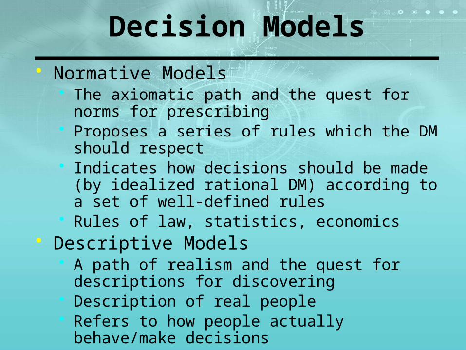
Decision Models

• Normative Models• The axiomatic path and the quest for norms for prescribing• Proposes a series of rules which the DM should respect • Indicates how decisions should be made (by idealized

rational DM) according to a set of well-defined rules• Rules of law, statistics, economics

• Descriptive Models• A path of realism and the quest for descriptions for

discovering• Description of real people• Refers to how people actually behave/make decisions • Characterizes what happens in the real world without

judgment of it • Pychology, behavioral sciences, marketing

Decision Models

• Constructive Models • Both normative and descriptive• Construct - create• The constructivist path and the quest for working hypothesis

for recommending

Constructing Decision Model

• Assessing performance values of alternatives w.r.t. attributes

• (If necessary) Determining relative importance of attributes

• Modeling the preference of DMs

Assessing Performance Values

• Determine how well each alternative achieves each attribute

• Performance value = score = rating = attribute level

Assessing Performance Values

• Objective evaluationNatural attribute is used

Quantitative

Independent of DM

Attributes are readily measured in terms of some natural physical unit

e.g. dollars or number of people

• Subjective evaluationConstructed attribute is used

Qualitative

Dependent on DM

No natural measuring scales exist e.g. beauty or convenience

Measurement Considerations

Performance values can be measured by: • Nominal scales• Ordinal scales• Interval scales• Ratio scales

Nominal Scales

• The lowest level in terms of the meaning conveyed• Nominal numbers are just numerical representations

for names• Used for identification purposes only and imply

nothing about ordering• e.g.Telephone number, Turkish Republic identification (ID) number: “Are

you older or better than someone else because your number is higher?

Ordinal Scales

• Ordinal numbers imply an order of ranking among elements

• The order may be increasing or decreasing• Ranking implies an ordering but nothing more: does

not imply anything about the differences between items

• We could order cities based on population by ranking the city with the highest population as #1 (or with lowest population)

Interval Scales

• Interval scale data has meaning about the differences between objects

• The unit as well as the origin on an interval scale can be assigned arbitrarily.

• Valid operations on an interval scale are multiplication and the addition of a constant

Interval Scales

• Statements concerning x1/x2 are meaningless as they depend on the choice of origin and unit.

• On the other hand statements concerning ratios of differences ((x1-x2)/(x3-x4)), are meaningful on interval scales since they are independent of both origin and the unit.

• Preference on utility scales and temperature on the Fahrenheit or Celcius scales (32+1.8*x transforms temperature from the Celcius to the Fahrenheit scale).

• If we have interval level data then we can infer that the interval between two objects with values of 20 and 5 (an interval of 15) is equivalent to the interval between two objects with values of 80 and 65

Ratio Scales

• Highest level meaning• The unit on a ratio scale can be chosen arbitrarily• The only valid operation (admissible transformation)

on a ratio scale is a change of unit (multiplying the scale by a positive constant).

• Adding a constant to a ratio scale is not a valid operation because zero point (origin) can not be defined arbitrarily on the scale.

Ratio Scales

• If x1 and x2 are two measurements on a ratio scale, statements concerning x1/x2 are independent of the unit chosen and are meaningful

• Length can be measured in inches, miles, meters…• Kelvin scale: the zero point of this scale is equivalent to -273.15 °C

Example for Scales

• Suppose the owner of a horse racing stable is interested in buying a particular horse. He studies the results.

• The number worn on the horse and jockey is nominal. It identifies the horse

• The finishing position for each horse is ordinal. e.g. the first place horse finished ahead of the second one.

• The number of lengths to the next finisher is an interval measure. Knowing that the horse finished first by 15 lengths as opposed to 5 lengths is important information.

• Suppose the horse finished first by 15 lengths in a 2.5 miles race. Is this as strong as finishing first by 15 lengths in a 0.5 miles race? More information would be conveyed if we knew the ratios of the times of the first and second place finishes.

• Alternative evaluations w.r.t. attributes are presented in a decision matrix• Entries are performance values • Rows represent alternatives• Columns represent attributes

Decision Matrix

Attributes

• Benefit attributesOffer increasing monotonic utility. Greater the attribute value the more its preference

• Cost attributesOffer decreasing monotonic utility. Greater the attribute value the less its preference

• Nonmonotonic attributesOffer nonmonotonic utility. The maximum utility is located somewhere in the middle of an attribute range

Global Performance Value

• If solution method that will be utilized is performance aggregation oriented, performance values should be aggregated.

• In this case• Performance values are normalized to eliminate

computational problems caused by differing measurement units in a decision matrix

• Relative importance of attributes are determined

Normalization

• Aims at obtaining comparable scales, which allow interattribute as well as intra-attribute comparisons

• Normalized performance values have dimensionless units

• The larger the normalized value becomes, the more preference it has

Normalization Methods

1. Distance-Based Normalization Methods

2. Proportion Based Normalization Methods (Standardization)

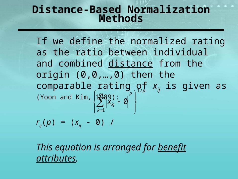
Distance-Based Normalization Methods

If we define the normalized rating as the ratio between individual and combined distance from the origin (0,0,…,0) then the comparable rating of xij is

given as (Yoon and Kim, 1989):

rij(p) = (xij - 0) /

This equation is arranged for benefit attributes.

Cost attributes become benefit attributes by taking the inverse rating (1/ xij)

ppm

kkjx

/1

1

0

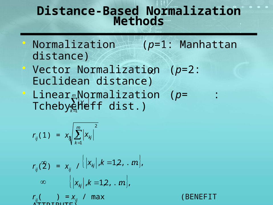
Distance-Based Normalization Methods

• Normalization (p=1: Manhattan distance)• Vector Normalization (p=2: Euclidean distance)• Linear Normalization (p= : Tchebycheff dist.)

rij(1) = xij /

rij(2) = xij /

rij( ) = xij / max (BENEFIT ATTRIBUTE)

rij( ) = min / xij (COST ATTRIBUTE)

m

kkjx

1

2

1

m

kkjx

,...,2,1 , mkxkj

,...,2,1 , mkxkj

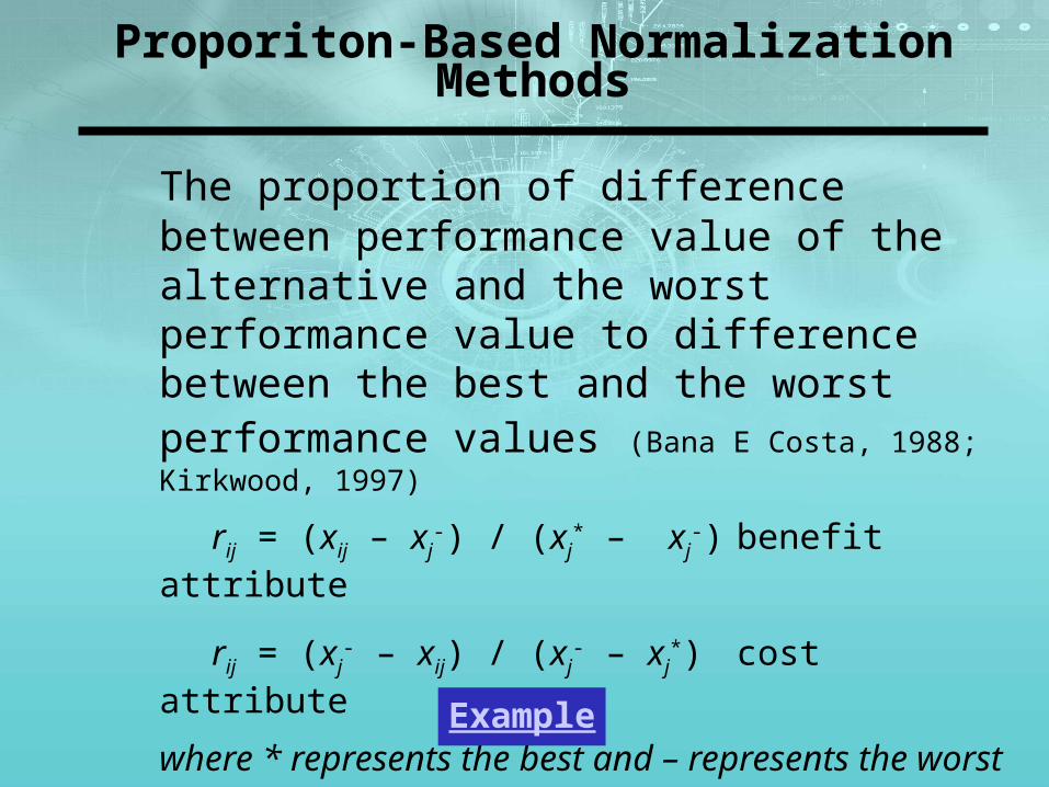
Proporiton-Based Normalization Methods

The proportion of difference between performance value of the alternative and the worst performance value to difference between the best and the worst performance values (Bana E Costa, 1988; Kirkwood, 1997)

rij = (xij – xj-) / (xj

* – xj-) benefit attribute

rij = (xj- – xij) / (xj

- – xj*) cost attribute

where * represents the best and – represents the worst

(best: max. perf. value for benefit; min. perf. value for cost or ideal value determined by DM for that attribute)

Example

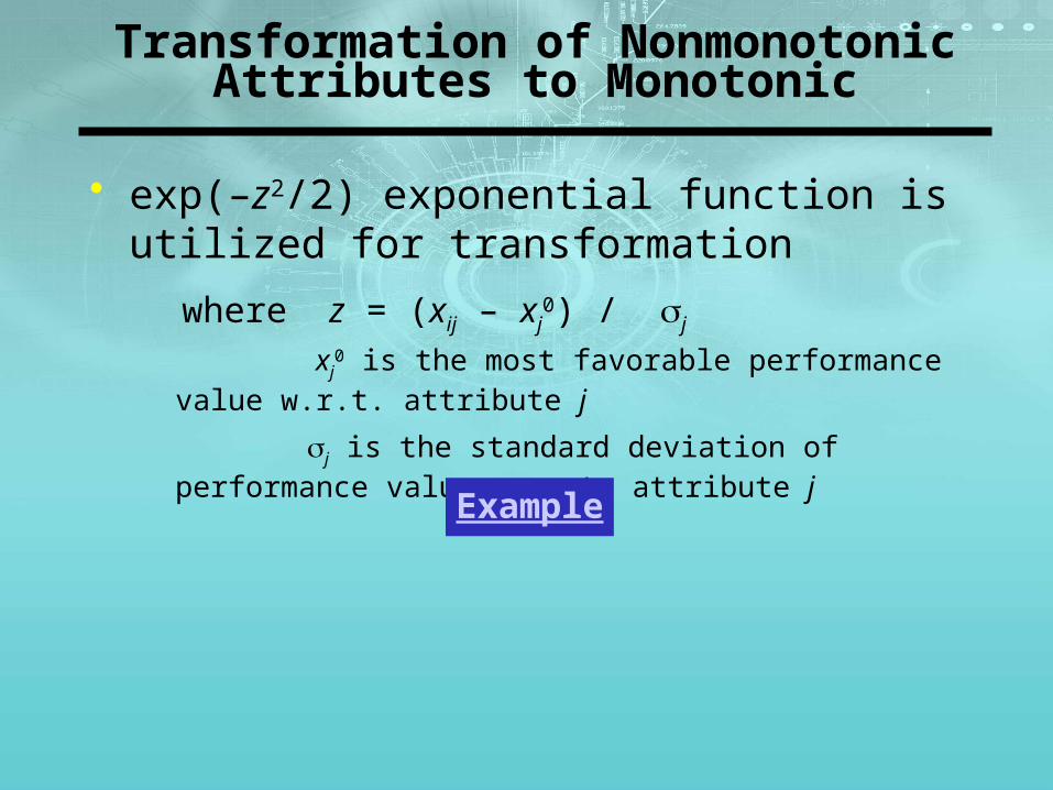
Transformation of Nonmonotonic Attributes to Monotonic

• exp(–z2/2) exponential function is utilized for transformation

where z = (xij – xj0) / sj

xj0 is the most favorable performance value w.r.t. attribute j

sj is the standard deviation of performance values w.r.t. attribute j

Example

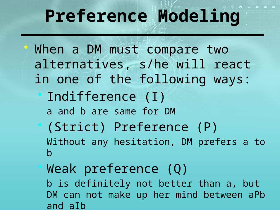
Preference Modeling

• When a DM must compare two alternatives, s/he will react in one of the following ways:• Indifference (I)

a and b are same for DM

• (Strict) Preference (P) Without any hesitation, DM prefers a to b

• Weak preference (Q) b is definitely not better than a, but DM can not make up her mind between aPb and aIb

• Incomparability (R) DM can not compare a and b (refusal or inability)

Attribute Weighting

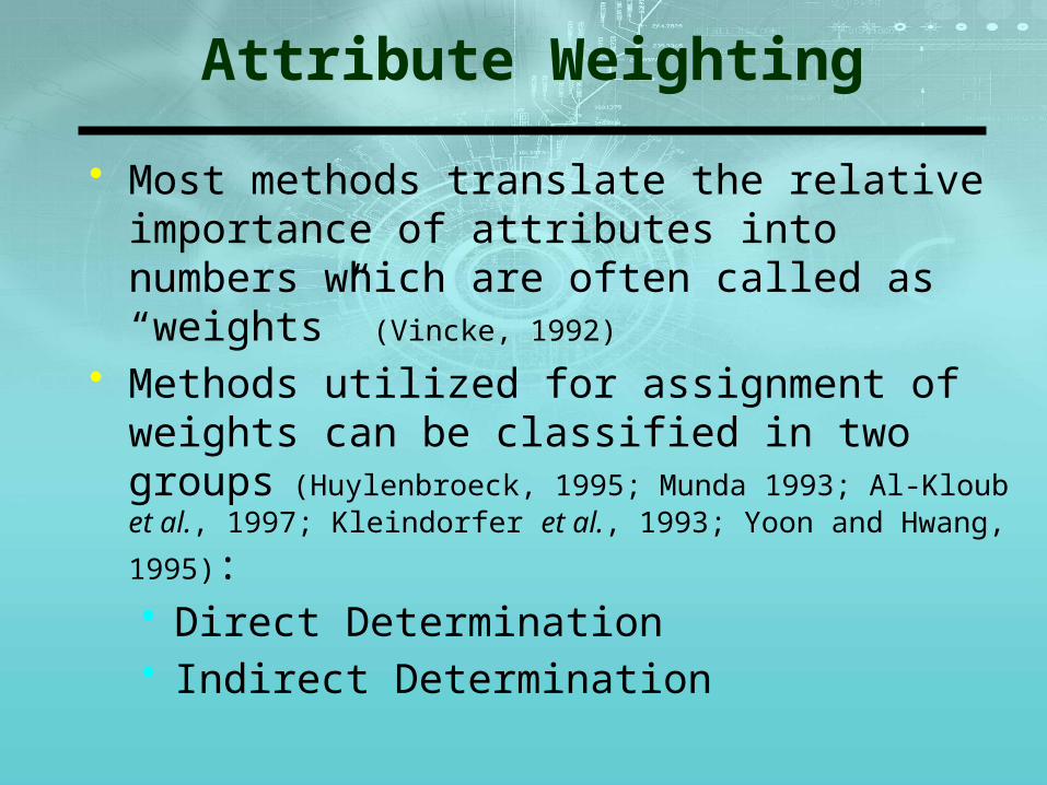
• Most methods translate the relative importance of attributes into numbers which are often called as “weights” (Vincke, 1992)

• Methods utilized for assignment of weights can be classified in two groups (Huylenbroeck, 1995; Munda 1993; Al-

Kloub et al., 1997; Kleindorfer et al., 1993; Yoon and Hwang, 1995):• Direct Determination• Indirect Determination

Weight Assignment Methods

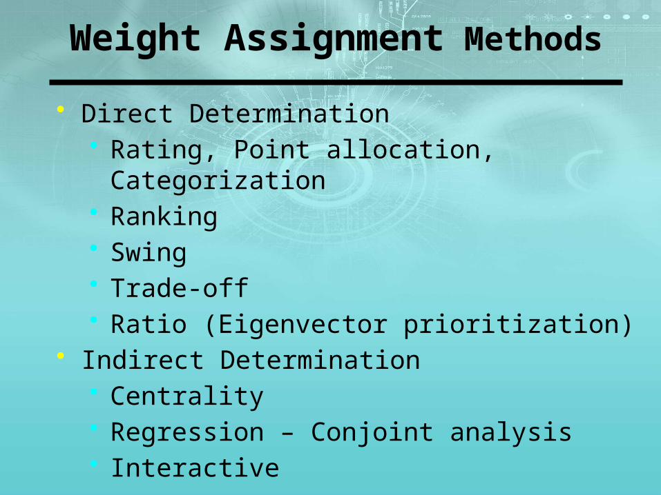
• Direct Determination • Rating, Point allocation, Categorization• Ranking• Swing• Trade-off• Ratio (Eigenvector prioritization)

• Indirect Determination

• Centrality• Regression – Conjoint analysis• Interactive

Rating

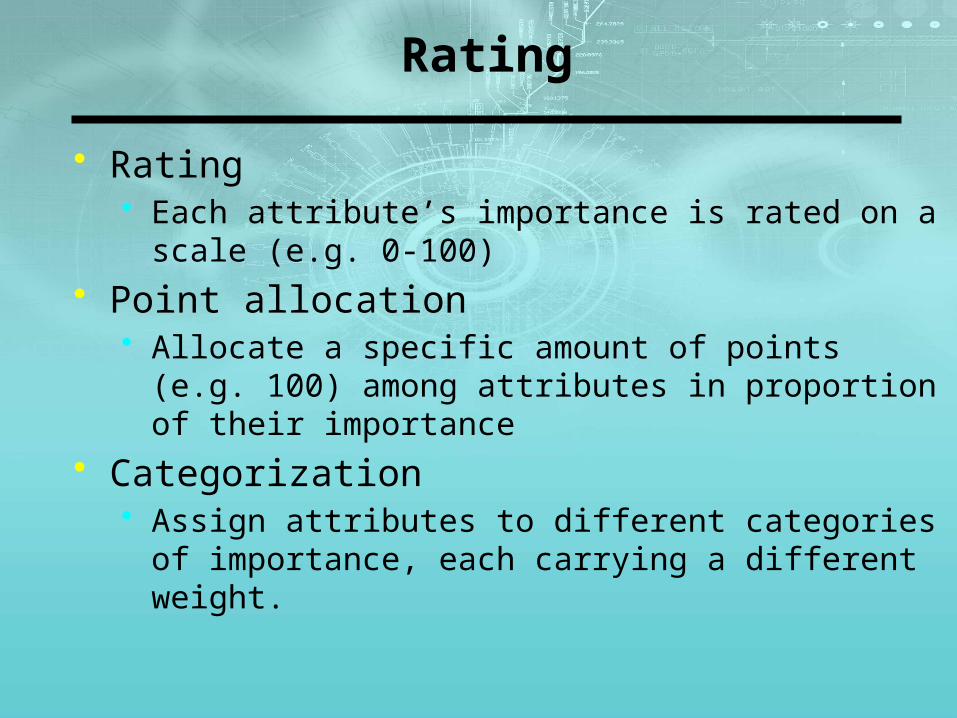
• Rating• Each attribute’s importance is rated on a scale (e.g. 0-100)

• Point allocation• Allocate a specific amount of points (e.g. 100) among

attributes in proportion of their importance

• Categorization• Assign attributes to different categories of importance, each

carrying a different weight.

Ranking

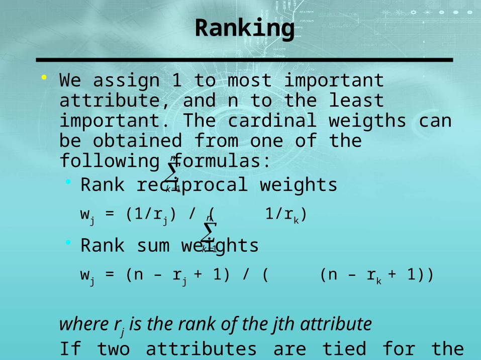
• We assign 1 to most important attribute, and n to the least important. The cardinal weigths can be obtained from one of the following formulas:• Rank reciprocal weights

wj = (1/rj) / ( 1/rk)

• Rank sum weights

wj = (n – rj + 1) / ( (n – rk + 1))

where rj is the rank of the jth attribute If two attributes are tied for the nth and (n+1)th place, the number (2n+1)/2 is assigned to both of them

n

k 1

n

k 1

Swing

• DM considers a hypothetical alternative where attributes are all at their worst value.

• S/he is then asked which of the attributes would most prefer to swing from its worst value up to its best value

• S/he is then asked which attribute s/he would swing up second and so on...

• After ranking the attributes in this manner, DM is asked to give the most important attribute a weight of 100, and then assign weights to the other attributes in proportion to the importance of their ranges.

Trade-off (Approach I)

• Consider a hypothetical alternative that has the least preferred level for all attributes.

• Now suppose that you could move one, and only one, of the attributes from its least preferred level to its most preferred level. Which would you move?

• Ask the same question for the remaining attributes. Continue until you have a ranking for all attributes

• Now consider the attribute that you most prefer to move (attribute 1) and compare it with the attribute that you second most prefer to move (attribute 2)

Trade-off (Approach I) ctd.

• Suppose that you could either move the second one all the way from its least preferred level to its most preferred level, or you could move the first one from its least preferred level to some intermediate level. Select this intermediate level for which you are indifferent between these two possibilities

• Then it must be true that the value for two hypothetical alternatives with performance values of above given possible hypothetical situations are equal:w1v1(xa1) + w2v2(x2

–) = w1v1(x1–) + w2v2(x2

*)

w1 k + w2 0 = w1 0 + w2 1 w1 k = w2

Trade-off (Approach II)

• Comparison of two alternatives described on two attributes (for the remaining attributes both alternatives have identical values). One alternative has the best outcome on the first and the worst outcome on the second attribute, the other has worst on the first and best on the second attribute

• By choosing the preferred alternative out of the two the DM decides on the most important attribute.

• Then the adjustment of attribute outcome in order to yield indifference between the two alternatives is done (either by worsening the chosen alternative in good outcome or improving the other one in the bad outcome)

Incomparability

• Incomparability appears even more frequently when contradictory opinions must be aggregated. If a decision is finally selected, it may be quite useful, during the decision aid step, to put forward clearly any lack of comparison between actions.

• On the other hand, when, given the information available, two possible actions turn out to be incomparable, this helps decision making since it amounts to putting forward some aspects of the problem at hand which deserve to be investigated.

Incomparability

e.g. FIFA World cup• After group matches, in each group first two teams qualify to second round

and last two teams are eliminated. 16 eliminated teams are incomparable with each other.

• At the second round, 16 qualified teams play two by two. Winners qualify to quarter final, losers are eliminated: 8 eliminated teams are incomparable But they are better than the eliminated teams at the first round.

• At quarter final 8 qualified teams play two by two. Winners qualify to semi final, losers are eliminated: 4 eliminated teams are incomparable But they are better than the eliminated teams at the first and second round.

• At semi final 4 qualified teams play two by two. Winners qualify to final, losers play with each other at the 3rd place playoff.

• Loser of 3rd place playoff is the 4th team of the tournament• Winner of 3rd place playoff is the 3rd team of the tournament• Loser of final is the 2nd team of the tournament• Winner of final is the 1st (champions) of the tournament

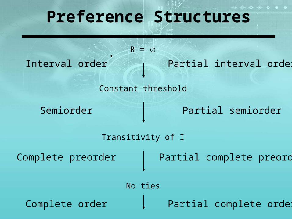
Preference Structures

Interval order

Semiorder

Complete preorder

Complete order

Partial interval order

Partial semiorder

Partial complete preorder

Partial complete order

R =

Constant threshold

Transitivity of I

No ties

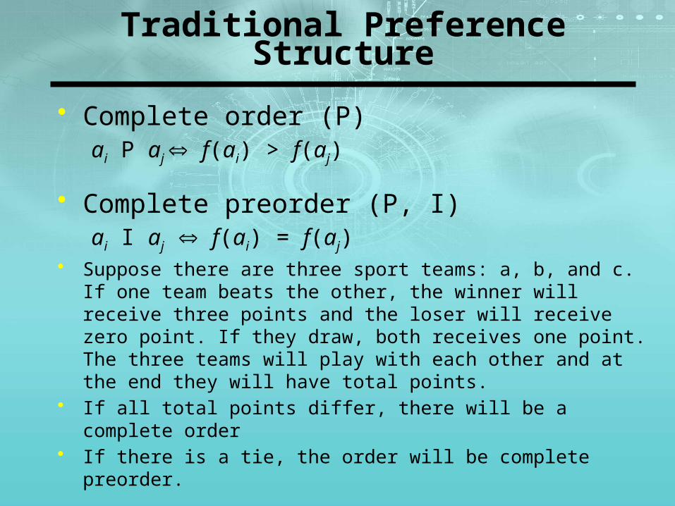
Traditional Preference Structure

• Complete order (P)ai P aj f(ai) > f(aj)

• Complete preorder (P, I)ai I aj f(ai) = f(aj)

• Suppose there are three sport teams: a, b, and c. If one team beats the other, the winner will receive three points and the loser will receive zero point. If they draw, both receives one point. The three teams will play with each other and at the end they will have total points.

• If all total points differ, there will be a complete order • If there is a tie, the order will be complete preorder.

Taking into account Indifference Threshold

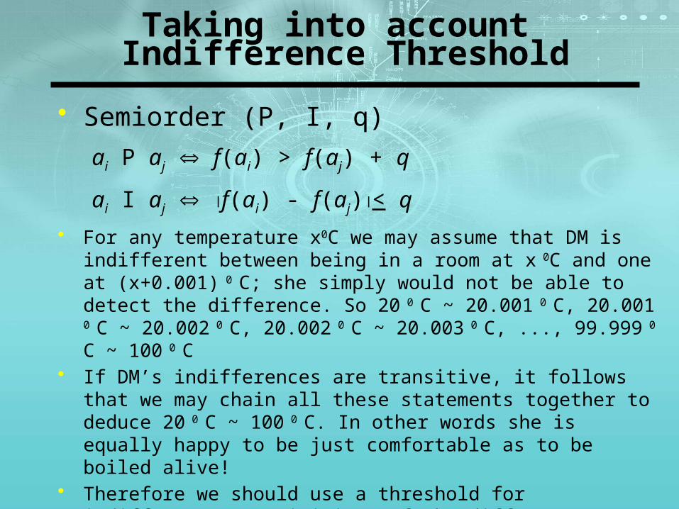
• Semiorder (P, I, q)

ai P aj f(ai) > f(aj) + q

ai I aj f(ai) - f(aj)< q

• For any temperature x0C we may assume that DM is indifferent between being in a room at x 0C and one at (x+0.001) 0 C; she simply would not be able to detect the difference. So 20 0 C ~ 20.001 0 C, 20.001 0 C ~ 20.002 0 C, 20.002 0 C ~ 20.003 0 C, ..., 99.999 0 C ~ 100 0 C

• If DM’s indifferences are transitive, it follows that we may chain all these statements together to deduce 20 0 C ~ 100 0 C. In other words she is equally happy to be just comfortable as to be boiled alive!

• Therefore we should use a threshold for indifference transitivity. If the difference between performance values of two alternatives is less than this threshold, the DM will be indifferent between these two alternatives. If the difference is greater than the threshold the DM prefers one to other.

Taking into account Indifference Threshold

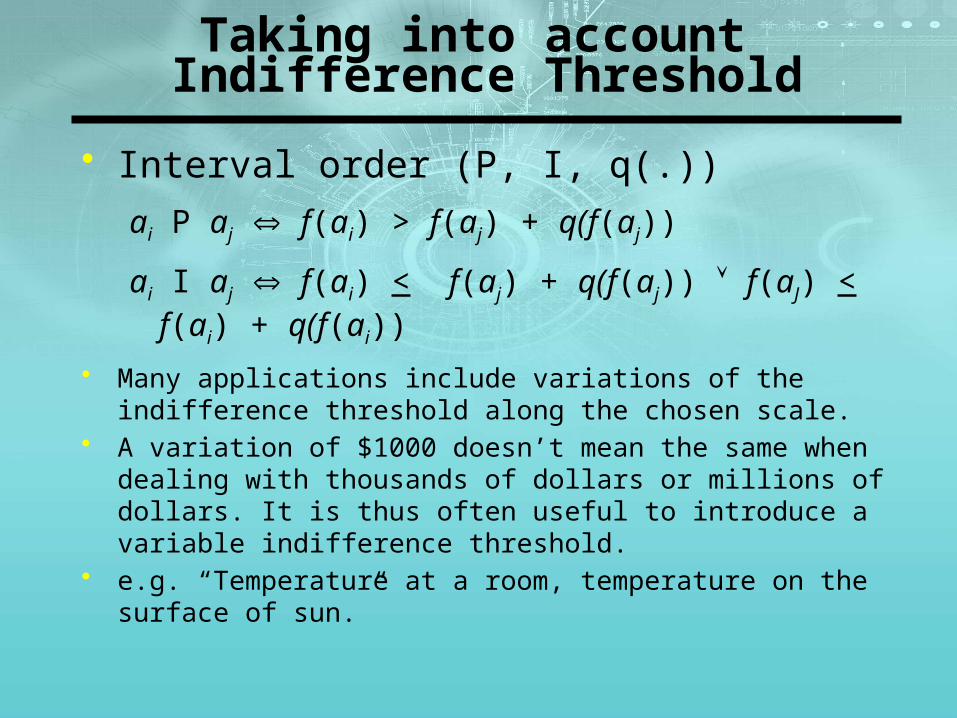
• Interval order (P, I, q(.))

ai P aj f(ai) > f(aj) + q(f(aj))

ai I aj f(ai) < f(aj) + q(f(aj)) f(aJ) < f(ai) + q(f(ai))

• Many applications include variations of the indifference threshold along the chosen scale.

• A variation of $1000 doesn’t mean the same when dealing with thousands of dollars or millions of dollars. It is thus often useful to introduce a variable indifference threshold.

• e.g. “Temperature at a room, temperature on the surface of sun.”

Taking into account Indifference & Preference Thresholds

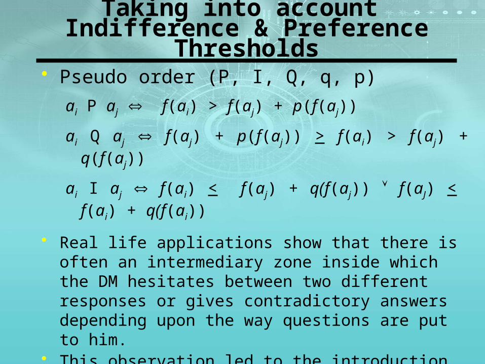
• Pseudo order (P, I, Q, q, p)

ai P aj f(ai) > f(aj) + p(f(aj))

ai Q aj f(aj) + p(f(aj)) > f(ai) > f(aj) + q(f(aj))

ai I aj f(ai) < f(aj) + q(f(aj)) f(aJ) < f(ai) + q(f(ai))

• Real life applications show that there is often an intermediary zone inside which the DM hesitates between two different responses or gives contradictory answers depending upon the way questions are put to him.

• This observation led to the introduction of a preference model:• An indifference threshold underneath which the DM shows

clear indifference • A preference threshold above which the DM is sure of

strict preference

Models including Incomparability

• Partial Order• Partial Preorder• Partial Semiorder• Partial Interval Order

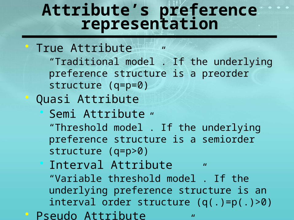
Attribute’s preference representation

• True Attribute“Traditional model”. If the underlying preference structure is a preorder structure (q=p=0)

• Quasi Attribute• Semi Attribute

“Threshold model”. If the underlying preference structure is a semiorder structure (q=p>0)

• Interval Attribute“Variable threshold model”. If the underlying preference structure is an interval order structure (q(.)=p(.)>0)

• Pseudo Attribute“Double threshold model”. If the underlying preference structure is a pseudo order structure (p>q>0)