Constraint-based Hybrid Cellular Automaton Topology

Optimization for Advanced Lightweight Blast Resistant Structure Development

by Dwight Hofstetter, Jr., Rahul Gupta, and Robert Bitting

ARL-TR-5820 November 2011 Approved for public release; distribution is unlimited.

NOTICES

Disclaimers The findings in this report are not to be construed as an official Department of the Army position unless so designated by other authorized documents. Citation of manufacturer’s or trade names does not constitute an official endorsement or approval of the use thereof. Destroy this report when it is no longer needed. Do not return it to the originator.

Army Research Laboratory Aberdeen Proving Ground, MD 21005-5066

ARL-TR-5820 November 2011

Constraint-based Hybrid Cellular Automaton Topology Optimization for Advanced Lightweight Blast

Resistant Structure Development

Dwight Hofstetter, Jr., Rahul Gupta, and Robert Bitting Weapons and Materials Research Directorate, ARL

Approved for public release; distribution is unlimited.

ii

REPORT DOCUMENTATION PAGE Form Approved OMB No. 0704-0188

Public reporting burden for this collection of information is estimated to average 1 hour per response, including the time for reviewing instructions, searching existing data sources, gathering and maintaining the data needed, and completing and reviewing the collection information. Send comments regarding this burden estimate or any other aspect of this collection of information, including suggestions for reducing the burden, to Department of Defense, Washington Headquarters Services, Directorate for Information Operations and Reports (0704-0188), 1215 Jefferson Davis Highway, Suite 1204, Arlington, VA 22202-4302. Respondents should be aware that notwithstanding any other provision of law, no person shall be subject to any penalty for failing to comply with a collection of information if it does not display a currently valid OMB control number.

PLEASE DO NOT RETURN YOUR FORM TO THE ABOVE ADDRESS. 1. REPORT DATE (DD-MM-YYYY)

November 2011 2. REPORT TYPE

Final 3. DATES COVERED (From - To)

June 2004–15 July 2011 4. TITLE AND SUBTITLE

Constraint-based Hybrid Cellular Automaton Topology Optimization for Advanced Lightweight Blast Resistant Structure Development

5a. CONTRACT NUMBER

5b. GRANT NUMBER

5c. PROGRAM ELEMENT NUMBER

6. AUTHOR(S)

Dwight Hofstetter, Jr., Rahul Gupta, and Robert Bitting

5d. PROJECT NUMBER

5e. TASK NUMBER

5f. WORK UNIT NUMBER

7. PERFORMING ORGANIZATION NAME(S) AND ADDRESS(ES)

U.S. Army Research Laboratory ATTN: RDRL-WMP-F Aberdeen Proving Ground, MD 21005-5066

8. PERFORMING ORGANIZATION REPORT NUMBER

ARL-TR-5820

9. SPONSORING/MONITORING AGENCY NAME(S) AND ADDRESS(ES)

10. SPONSOR/MONITOR’S ACRONYM(S) 11. SPONSOR/MONITOR'S REPORT NUMBER(S)

12. DISTRIBUTION/AVAILABILITY STATEMENT

Approved for public release; distribution is unlimited. 13. SUPPLEMENTARY NOTES

14. ABSTRACT

Optimization of blast-resistant structures for combat vehicles allows for maximum protection when constrained by additional weight. Livermore Software Topology and Shape Computations (LS-TaSC) optimization software is a constraint-based hybrid cellular-automaton tool that could be used to design optimum solutions. This software takes into account size, shape, topology, and topometry (changing of element properties on an element-by-element basis). The optimization is achieved by designing for a uniform internal energy density while constraining responses such as plastic strains and Von Mises stresses. New constraints added to the LS-TaSC optimization software allow a user to specify a maximum deflection with regard to a specified mass fraction and casting direction. If a realistic mass fraction and deflection constraint combination is specified, the model will be successfully altered until a uniform internal energy density is met, thereby minimizing mass and deflection. Another beneficial feature is the addition of a casting feature, which allows users to specify the face that is to be optimized. This report explores the utility of the enhanced LS-TaSC optimization software and its applications to the U.S. Army Research Laboratory (ARL) researchers for creating optimum lightweight blast-resistant structures for future and current vehicles. 15. SUBJECT TERMS

LS-TaSC, LS-OPT/Topology, hybrid cellular automaton

16. SECURITY CLASSIFICATION OF: 17. LIMITATION OF ABSTRACT

UU

18. NUMBER OF PAGES

44

19a. NAME OF RESPONSIBLE PERSON

Dwight Hofstetter, Jr. a. REPORT

Unclassified b. ABSTRACT

Unclassified c. THIS PAGE

Unclassified 19b. TELEPHONE NUMBER (Include area code)

(410) 306-2091 Standard Form 298 (Rev. 8/98) Prescribed by ANSI Std. Z39.18

iii

Contents

List of Figures iv

List of Tables v

Acknowledgments vi

1. Introduction/Background 1

1.1 Topology .........................................................................................................................1

1.2 Topometry .......................................................................................................................2

1.3 Hybrid Cellular Automata (HCA) ...................................................................................3

1.4 Criteria for Evaluating Elements .....................................................................................5

1.5 Deflection Constraint ......................................................................................................7

1.6 Casting Constraint ...........................................................................................................7

2. Analysis/Calculations 8

2.1 Operation .........................................................................................................................8

2.1.1 LS-OPT/Topology ...............................................................................................9

2.1.2 LS-TaSC ............................................................................................................10

2.2 Procedure .......................................................................................................................11

3. Results and Discussion 13

3.1 LS-OPT/Topology vs. LS-TASC ..................................................................................13

3.1.1 LS-OPT/Topology (Unconstrained) ..................................................................13

3.1.2 LS-TaSC (Without Constraints) ........................................................................15

3.2 LS-TaSC (Positive Z-axis Casting Constraint with Deflection Constraint)..................16

4. Summary and Conclusions 18

5. References 20

Appendix A. Unconstrained Single Plate 23

Appendix B. Constrained Single Plate with Top Pressure Plate (No Contact Defined) 25

Appendix C. Constrained Single Plate with Top Pressure Plate (With Contacts Defined) 29

Distribution List 31

iv

List of Figures

Figure 1. Hybrid cellular automata based topology optimization example (3, 4). .........................1

Figure 2. Topometry optimization (6). ...........................................................................................2

Figure 3. Topology/topometry comparison (6). ..............................................................................3

Figure 4. Hybrid cellular automata-based topology optimization flowchart (3, 4, 9). ...................4

Figure 5. Casting constraint options (4). .........................................................................................7

Figure 6. Casting faces along an axis selected for removal. ...........................................................7

Figure 7. LS-OPT/topology vs. LS-TaSC.......................................................................................8

Figure 8. First simulation model. ..................................................................................................12

Figure 9. Second simulation model. .............................................................................................13

Figure 10. LS-OPT/topology optimization progress. ...................................................................14

Figure 11. LS-OPT/topology optimized plate. .............................................................................14

Figure 12. LS-OPT/Topology density redistribution (left) and total internal energy density (right). ......................................................................................................................................15

Figure 13. LS-TaSC optimization progress (without constraints). ...............................................15

Figure 14. LS-TaSC optimized plate (without constraints). .........................................................16

Figure 15. LS-TaSC (without constraints) mass (left) and mass fraction (right). ........................16

Figure 16. LS-TaSC optimization progress (with constraints). ....................................................17

Figure 17. LS-TaSC optimized plate (with constraints). ..............................................................17

Figure 18. LS-TaSC (with constraints) mass redistribution (left), mass fraction (middle), and deflection (right). .....................................................................................................................18

Figure A-1. Initial simulation model. ...........................................................................................23

Figure B-1. LS-TaSC deflection constraint iteration 11. ..............................................................25

Figure B-2. LS-TaSC deflection constraint optimization process. ...............................................26

Figure B-3. LS-TaSC deflection constraint instability. ................................................................26

Figure B-4. LS-TaSC deflection constraint optimization process instability. ..............................27

Figure C-1. LS-TaSC deflection constraint optimization CONTACT_AUTOMATIC_SINGLE_SURFACE. ...............................................................29

Figure C-2. LS-TaSC deflection constraint optimization CONTACT_ERODING_SINGLE_SURFACE. .....................................................................30

v

List of Tables

Table 1. Plate properties. ..............................................................................................................12

Table 2. Program comparison. ......................................................................................................18

Table A-1. Plate properties. ..........................................................................................................23

vi

Acknowledgments

We wish to acknowledge the support of Mr. Luke Harper (SURVICE Engineering Inc).

1

1. Introduction/Background

Physical nonlinearities are abundant in the process of a blast event (1). Topology optimization in the context of impact analysis is a very complex problem due to the nonlinear interactions involving material, geometry, and transient boundary conditions. Due to the high computational cost and the lack of sensitivity information, conventional methods are not practical for these nonlinear topology optimization problems (2). Livermore Software (LS)-OPT/Topology software was one of the first optimization software packages to explore the field of large deformation, nonlinear problems with dynamic loading. The recently released second version, the LS Topology and Shape Computations (LS-TaSC), incorporates several new features added to the same core engine. The most valuable addition for the U.S. Army Research Laboratory (ARL) engineer is the deflection constraint as a global response.

1.1 Topology

LS-TaSC optimizes the size, shape, topometry, and topology of a model through reconstruction. Topology is an important factor in this process, because it deals with the material as well as the material properties. Figure 1 shows an example of the topology optimization process. Topology is defined as a field in mathematics that focuses on an object’s spatial properties as they are preserved during deformations such as bending or twisting but not to include tearing (5). LS-TaSC minimizes the size and optimizes the shape of the piece by removing cells from which it is made; yet, the program does not cut the model into more than one piece. Design for structural topology optimization is a method of distributing material within a design domain of prescribed dimensions. This domain is discretized into a large number of cells. The optimization algorithm adds, removes, or maintains the amount of material. The resulting structure maximizes a prescribed mechanical performance while satisfying functional and geometric constraints (1).

Figure 1. Hybrid cellular automata based topology optimization example (3, 4).

2

1.2 Topometry

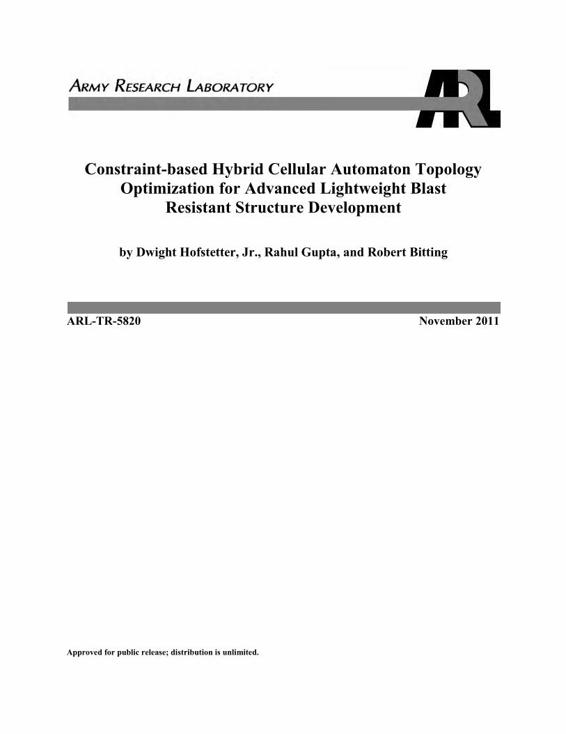
Topometry optimization involves finding a thickness function within the design domain so that the resulting design will sustain the applied load or impact as efficiently as possible. Figure 2 demonstrates an example of the topometry optimization process where material thickness increases as the color changes from blue to red. Most often, the thickness function is discretized according to a finite element mesh (7). Topometry optimization is typically used to find the distribution of dimensions of a structure. In analysis, Young’s modulus is always constant but the physical dimension can be changed. The method may add material to a structure and an initial design is required for it to proceed with the optimization. The method is also ideal for analyzing composite structures (6). Essentially, an ideal structure can be designed, but size and initial dimensions do not play a large factor. Element properties are changed on an element-by-element basis, which allows the LS-TaSC program to design shell thicknesses (4). Figure 3 illustrates the difference between topology and topometry.

Figure 2. Topometry optimization (6).

3

Figure 3. Topology/topometry comparison (6).

1.3 Hybrid Cellular Automata (HCA)

A cellular automaton (CA) is a collection of “colored” or distinct state cells on a grid of a specified shape that evolves through a number of discrete time steps according to a set of rules based on the states of neighboring cells (8). However, for the structural optimization problems, the state of a cellular automaton is defined by rules that combine the local neighborhood information with the field variables that are calculated globally (3, 4, 9), which makes the method a hybrid. The globally calculated field variables refer to those held within the entire model. Control rules drive a defined field variable to an optimum state or set point. The expression for the field variable and the value of the set point are derived from the optimal conditions of the structural design problem. A local rule iteratively updates the modulus at each cell based on the difference between a current stress value and a target value. Evolutionary rules based on the growing/reforming procedure are used to fine-tune the structure. Cells with a low elastic modulus are removed, while cells with high elastic modulus create a new cell in an empty surrounding space (10). Among different topology optimization algorithms, the HCA method has proven to be efficient and robust in problems involving large, plastic deformations (1). The internal energy density of each cell must first be found followed by neighborhood definitions as is illustrated by equations 1 and 2.

4

Internal energy density (11) is

where

(Ui) = internal energy density of the ith element,

Σ (sigma) = stress, and

ε = strain.

Internal energy density as seen by HCA (3, 4, 9) is

,

where

(Ui) = energy density of ith cellular automata lattice and

n = amount of neighbors/adjacent cells

In the context of HCA, the field variables are subjected to the neighborhood update rule and subsequently, the design variables are updated. The process is iterated until equilibrium is established among all state variables (3, 4, 9) as can be seen in figure 4.

Figure 4. Hybrid cellular automata-based topology optimization flowchart (3, 4, 9).

5

1.4 Criteria for Evaluating Elements

The topology design problem is defined by the allowable geometric domain, how the part will be used, and the properties of the part. A design variable is directly linked to each material element such that each cell has its own material model (12). The objective for optimization is to obtain a maximum uniform internal energy density among all these elements (9, 13). The internal energy density is found and used as a measure of the extent to which a certain finite element contributes to the total internal energy, and thus, to the importance of the element from a topological point of view. In order to distribute the absorbed energy in a structure, the internal energy density should be evenly distributed among the various finite elements of the design domain. To ensure the even distribution of the internal energy density, a target internal energy density is evaluated after each iteration and all the elemental internal energy densities are compared with this target value (11). The formulation of the optimization problem can be seen in equations 3 and 4.

The optimization problem (3, 4, 9) is given as

,

where

U = energy density of the ith element, w = weighted parameter, U* = internal energy set point, L = amount of load cases, and x = relative density/design variable.

The optimization problem constraints (3, 4, 9) are given as

,

where

Vi = volume of the ith element, ρ = density of the material, M* = updated mass of the structure, and x = relative density/design variable.

The solid isentropic material with a penalization model is used to interpolate the material properties as can be seen in the equations 5–7, and 8.

6

Density (3, 4, 9) is

,

ρ = density of the material, 0 = refers to the base material properties, and x = relative density/design variable.

Young’s Modulus (3, 4, 9) is

,

where

E = Young’s modulus, 0 = refers to the base material properties, x = relative density/design variable, and p = material linearity exponent.

The Yield Stress (3, 4, 9) is given as

,

where

0 = refers to the base material properties, x = relative density/design variable, and q = material nonlinearity exponent.

The Strain Hardening Modulus (3, 4, 9) is given as

where

Eh = strain hardening modulus, 0 = refers to the base material properties, x = relative density/design variable, and q = material nonlinearity exponent.

Internal energy most often consists of elastic and plastic deformations. By decreasing the mass of the entire model, an increase in the total internal energy per total mass can be obtained (12). When the blast pressure wave hits the targeted structure, the kinetic energy is transformed into strain energy inside the solid medium. Maximum attenuation is reached when strain energy is maximized. This condition is satisfied when strain energy is uniformly distributed in the design domain (1). Several constraints can be set such as the number of design iterations, the desired mass fraction, the minimum density fraction before deleting an element, and global constraints.

7

1.5 Deflection Constraint

Deflection constraints consider the stiffness and reaction forces contained within a structure. LS-TaSC will add material to a part so that rigidity will increase, preventing it from deflecting beyond the specified limit. However, if reaction forces on the object are too large, then material must be removed. In the case of conflict between specified global constraints, a compromise is chosen to give each constraint an equal amount of violations/agreements. The algorithm for this feature searches for the mass of the structure (3).

1.6 Casting Constraint

The manufacturing process of casting allows intricate features to be created on a part’s face, as can be seen in figure 5. Casting direction is required for a casting constraint. The direction can be one or two sided on the x-, y-, or z-axis of a solid model. This is the direction in which the material will be removed. The casting definitions are implemented as inequality constraints requiring certain variables to be larger than others according to the casting direction. The casting direction must be on the symmetry planes and only one casting definition may be defined per part (3). When the casting direction is set, any surface that faces the casting direction will be optimized, as can be seen in figure 6.

Figure 5. Casting constraint options (4).

Figure 6. Casting faces along an axis selected for removal.

8

2. Analysis/Calculations

2.1 Operation

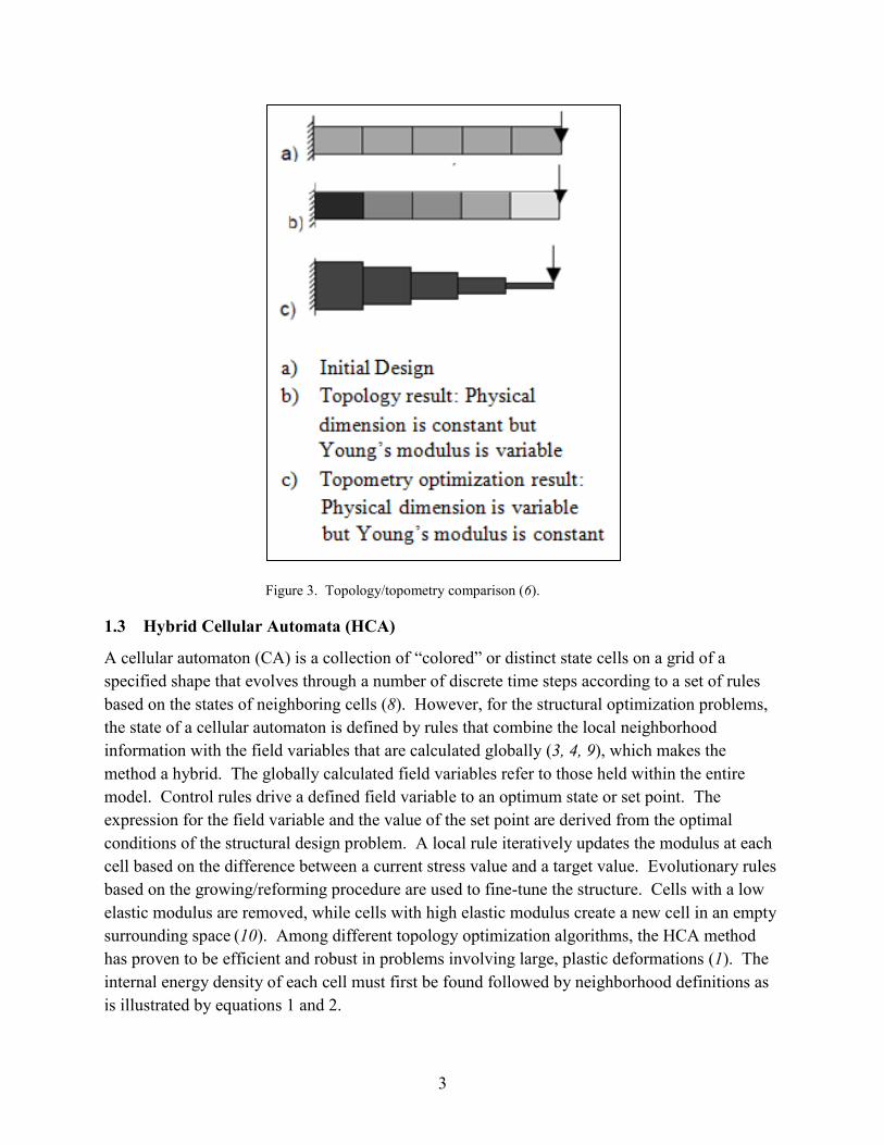
Version 1 (LS-OPT/Topology) and version 2 (LS-TaSC) are based on the same core engine. However, several additions to the solver have been made, which are reflected in the graphical user interfaces (GUI). The changes are illustrated in figure 7. Panels have been reorganized and divided to better group certain variables. The Analysis Type has been removed from the cases panel due to the fact that the program’s most desirable feature is that it can analyze nonlinear problems. Linear problem analysis is typically not desired by users.

Figure 7. LS-OPT/topology vs. LS-TaSC.

9

2.1.1 LS-OPT/Topology

2.1.1.1 LS-Prepost

One of the required pieces for the operation of LS-OPT/Topology is an initial model created in LS-Prepost, which sets the limit constraints for the final optimized piece. The model must be created using the PIECEWISE_LINEAR_PLASTICITY material with eight-noded solid elements. Models cannot be subjected to a pressure loading over the face that will be optimized to prevent load loss when elements are removed. A resolution to this is the addition of a part that will not be optimized between the original part and the pressure loading. This will ensure that the pressure is evenly distributed even when elements are removed.

2.1.1.2 Opening/Info

LS-OPT/Topology’s GUI can be opened from the file pull-down menu. When the GUI window appears, the first item the user sees is the Info panel with license and working directory information as well as a place to insert a problem description. Any desired reference name can be placed in the problem description.

2.1.1.3 Cases

The next tab, Cases, is where all of the input file information are inserted. First, a user must select the “new” button at the bottom of the window. In the Edit Cases pop-up window, the General tab is selected. The user must create a name for the case as well as specify the weight, which is simply a scaling factor if multiple loads are used. One of two types of analysis need to be selected: linear or nonlinear. At this point, the model that was created in LS-PrePost can be imported into the program by browsing the input file name. LS-OPT/Topology requires a LS-DYNA executable to solve, which can be specified by browsing the execution command. The Scheduling default settings are sufficient for this experiment. When done, the user can select the “ok” button to finish the selection.

2.1.1.4 Problem

After selecting the Problem panel, a design part ID needs to be specified. The design-part ID is a means of referring to the place where all elements in the design domain have been placed in the LS-DYNA input deck. This reference number can be found in the model’s viewing window. On the bottom of the Problem panel is a box labeled mass fraction. This refers to the amount of material that is desired to be eliminated, where a value of 1 would conserve the original model and a value of zero would remove the entire model.

2.1.1.5 Method

Under the Method panel is the termination criteria. The most often used termination criterion is the number of design iterations. LS-OPT/Topology will terminate when this number of iterations is reached. The convergence tolerance terminates the program when the topology begins making few changes. This is controlled by the density redistribution history variable. The proximity

10

tolerance is based on the uniformity of neighboring elements. Elements with a density less than the minimum density fraction specified in the minimum density fraction box are deleted on a given iteration.

2.1.1.6 Solution

After selecting the Run panel, the only visible button is “run”. Upon clicking on this button, the user is prompted to save the solution. A storage location and a name are given to the run, “ok” is selected, and the solution begins. Each iteration has a percent completion bar displayed at the top of the page and an engine output display is visible at the bottom. At any time, the run can be stopped and deleted or stopped to be restarted later.

2.1.1.7 View

The View panel allows a user to see a graph of the density redistribution as well as a graph of the total internal energy density. As the number of iterations increases, the graphs readjust to show the new data. From the View panel, a user can also open LS-Prepost to post process the iterations, displaying the changes that have been made to the model. The iterations can be viewed individually or simultaneously with up to six iterations being shown at a time.

2.1.2 LS-TaSC

2.1.2.1 LS-Prepost

An LS-Prepost model also needs to be created for LS-TaSC to analyze. The model can nearly be the same as the one created for LS-OPT/Topology. However if constraints are to be set in LS-TaSC, the ASCII_Option and History_Node needs to be altered in LS-Prepost. The model must be created using the PIECEWISE_LINEAR_PLASTICITY material with eight-node solid elements or four-node tetrahedral elements. Shell elements may be four- or three-node shell elements. The triangular elements must be specified as four-node shell elements by specifying the last node twice (4).

2.1.2.2 Opening/Info/Cases

The opening of LS-TaSC is identical to the opening of LS-OPT/Topology. The Info and Cases tabs are also indistinguishable.

2.1.2.3 Parts

The Parts panel essentially replaced the Problem panel of LS-OPT/Topology. The design part ID and the mass fraction are specified first. Then, the neighbor radius and minimum variable fraction can be specified, which were previously in the Methodology panel of LS-OPT/Topology. At the bottom of the panel, a part geometry section was added, where a user can specify an extrusion set ID, symmetry plane, cast direction, and a coordinate system ID. Each of these is chosen via an individual icon. The desired extrusion plane, symmetry plane, and casting direction need to be selected. A maximum of three geometry definitions are possible, and they

11

must be orthogonal to each other. The extrusion direction must be on the symmetry planes, the casting direction must be on the symmetry planes, the extrusion directions must be orthogonal to the casting directions, and the symmetry planes must be orthogonal (4).

2.1.2.4 Constraints

The Constraints panel is the primary addition to the software. When opened, the user sees a blank page, and then selects to create a new constraint. Constraint types include USERDEFINED, NODOUT, or RCFORC. At the bottom of the page is a location to place the name for the constraint and actual constraint values. USERDEFINED allows a user to enter a response command directly. NODOUT requires an Identifier Type such as ID or Heading, its Displacement direction, which value to select, and filtering. RCFORC requires an interface ID, selection of force type, which value to select, and filtering.

2.1.2.5 Completion

The Completion panel is a branch of the former Methodology panel and simply asks for the number of iterations and minimum mass fraction.

2.1.2.6 Run/View

Both the Run and View panels mirror their counterparts in LS-OPT/Topology.

2.2 Procedure

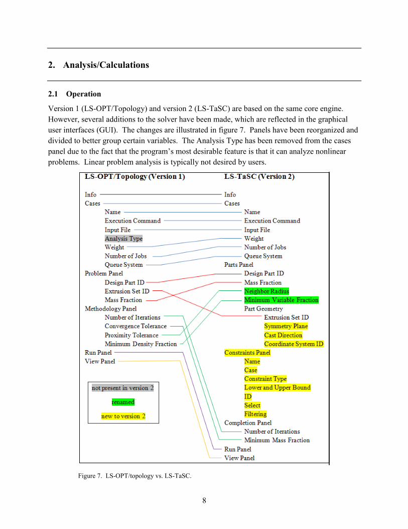
It is hypothesized that LS-TaSC can optimize a plate with no optimization parameter constraints in fewer iterations than LS-OPT/Topology requires due to its improved algorithms. To test the hypothesis, a plate under pressure loading was modeled. Figure 8 demonstrates the model with dimension, loading, boundary conditions, and material properties. The plate was 1.2- × 1.2- × 0.15-m (48- × 48- × 6-in) with boundary conditions set along opposite edges with a pressure loading in order to imitate a blast load from an underbody improvised explosive device (IED). The mesh density was 1.27 cm (0.5 in). It was desired to place a pressure loading directly on the piece but this was not feasible to be used alongside LS-OPT/Topology or LS-TaSC (see appendix A). Since pressure loading on a piece in either LS-OPT/Topology or LS-TaSC will result in an error termination due to negative volume when elements are removed, a thinner, non-evaluated 2.5-cm (1-in) plate was added to the top to convert the pressure loading to a surface-to-surface loading. Table 1 displays the properties given to the plate. The initial model was solved using LS-OPT/Topolgy and later with LS-TaSC (to compare the relative performance). The number of iterations was set to 100.

12

Figure 8. First simulation model.

Table 1. Plate properties.

Mass Density (kg/m^3)

Young’s Modulus (Pa)

Poisson’s Ratio Yield Stress (MPa)

7850 2.07E + 11 0.27 0 EPS1 EPS2 EPS3 EPS4

0 0.0055 0.0152 0.0248 EPS5 EPS6 EPS7 EPS8

0.0627 0.16 0.28 0.42 ES1 (Pa) ES2 (Pa) ES3 (Pa) ES4 (Pa)

7.922 × 10^8 9.23 × 10^8 9.61 ×10^8 9.830 × 10^8 ES5 (Pa) ES6 (Pa) ES7 (Pa) ES8 (Pa)

1.029 × 10^8 1.077 × 10^9 1.098 × 10^9 1.104 × 10^9

It is also hypothesized that using LS-TaSC to design and test armor plates with both deflection and casting constraints will generate a much different yet more practical model than LS-OPT/Topology or LS-TaSC without deflection constraints are able to. The same properties illustrated by table 1 were used. The displacement was set under the Constraints panel to be ‒0.25 as the last value in the z component direction. For this run, the HISTORY_NODE in the model had to be set to the corresponding reference node to obtain an output for the node. Figure 9 shows that the reference node was set in the center on the top of the plate that would not be optimized. The reference node was placed on the top of the plate that was not to be optimized so that it would not be removed. The time interval between outputs was set to 0.005 with a flag for binary file of 2 under NODOUT. Solely adding a deflection constraint may cause LS-TaSC to optimize a plate in a manner that may result in instabilities (see appendix B). A CONTACT_ AUTOMATIC_SINGLE_SURFACE was added to the model solely out of good practice (see

13

appendix C). Since removing material away from a contact surface seems to cause instabilities, a casting constraint in the positive z direction was added to the LS-TaSC run file and was allowed to run as can be seen in figure 9.

Figure 9. Second simulation model.

3. Results and Discussion

3.1 LS-OPT/Topology vs. LS-TASC

3.1.1 LS-OPT/Topology (Unconstrained)

Deflection constraints were not initially assigned to the problem solved by both LS-OPT/Topology and LS-TaSC, which resulted in similar shapes with small differences. Since a plate that was not to be optimized was placed between the pressure loading and the plate that was optimized, negative volume did not occur when mass was removed from the optimized plate.

The LS-OPT/Topology solution converged after 66 iterations. Figure 10 provides a visual of the optimization progress through a 3 × 2 matrix (left to right and back to front). Figure 11 displays the final form the optimized plate: top, bottom, and a centerline cross-sectional view. The top and bottom views are shaded where elements were removed. As can be seen, these cuts were primarily symmetric along the center axis. The top displayed jagged cuts where the bottom showed smooth and linear cuts. The density redistribution initially rapidly rose to 0.073 then steadily converged to zero (figure 12, graph 1). The total internal energy density started at 3.84e + 12, decreased to 2.94e + 12 on the fourth iteration, then rose to 3.2e + 12 on the fortieth iteration, and leveled off to 3.18e + 12 (figure 12, graph 2).

14

Figure 10. LS-OPT/topology optimization progress.

Figure 11. LS-OPT/topology optimized plate.

15

Figure 12. LS-OPT/Topology density redistribution (left) and total internal energy density (right).

3.1.2 LS-TaSC (Without Constraints)

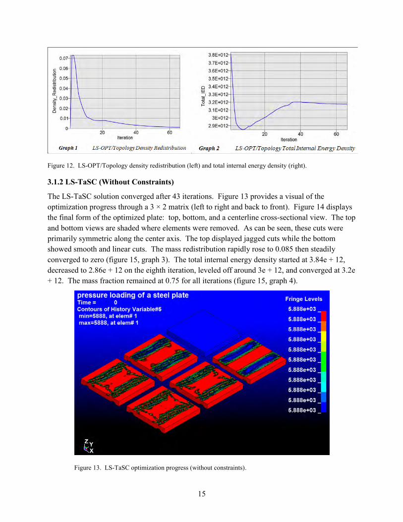
The LS-TaSC solution converged after 43 iterations. Figure 13 provides a visual of the optimization progress through a 3 × 2 matrix (left to right and back to front). Figure 14 displays the final form of the optimized plate: top, bottom, and a centerline cross-sectional view. The top and bottom views are shaded where elements were removed. As can be seen, these cuts were primarily symmetric along the center axis. The top displayed jagged cuts while the bottom showed smooth and linear cuts. The mass redistribution rapidly rose to 0.085 then steadily converged to zero (figure 15, graph 3). The total internal energy density started at 3.84e + 12, decreased to 2.86e + 12 on the eighth iteration, leveled off around 3e + 12, and converged at 3.2e + 12. The mass fraction remained at 0.75 for all iterations (figure 15, graph 4).

Figure 13. LS-TaSC optimization progress (without constraints).

16

Figure 14. LS-TaSC optimized plate (without constraints).

Figure 15. LS-TaSC (without constraints) mass (left) and mass fraction (right).

3.2 LS-TaSC (Positive Z-axis Casting Constraint with Deflection Constraint)

The LS-TaSC solution with constraints ended after 49 iterations. Figure 16 provides a visual of the optimization progress through a 3 × 2 matrix (left to right and back to front). Figure 17 displays the final form of the optimized plate: top, bottom, and centerline cross-sectional view from both the front and side views. The top and bottom views are shaded where elements were removed. As can be seen, parallel holes were cut symmetric about the center axis. The bottom view displayed one large scoop of elements taken from the center. The mass redistribution

Graph 3 LS-TaSC (without constraints) Mass

Redistribution Graph 4 LS-TaSC (without constraints) Mass Fraction

17

rapidly rose to 0.1 then steadily converged to 0 (figure 18, graph 5). The total internal energy density started at 3.474e + 12, increased to 7.713e + 12 on the twelfth iteration, and then decreased and converged at 6.118e + 12. The mass fraction fell to 0.380 at the fourteenth iteration then steadily increased and converged at 0.505 (figure 18, graph 6). The deflection of the plate reached –0.27 on iteration 15 then rose to the desired level of –0.25.

Figure 16. LS-TaSC optimization progress (with constraints).

Figure 17. LS-TaSC optimized plate (with constraints).

18

Figure 18. LS-TaSC (with constraints) mass redistribution (left), mass fraction (middle), and deflection (right).

Table 2 displays that the largest variation between the LS-TaSC (without constraints) and LS-OPT/Topology solutions was a 0.04 final density/mass distribution difference, but the vertical deformations and the internal energy densities were almost identical. Table 2 also shows that LS-TaSC (with constraints) resulted in a percent reduction that was greater than that of the previous runs and in turn was allowed to reach a specified vertical deformation that was much lower than the previous runs without constraints. Due to this, the internal energy density in the LS-TaSC (with constraints) solution was higher.

Table 2. Program comparison.

Program Vertical

Deformation (m)

Initial Mass (kg)

Optimized Mass (kg)

% Reduction —

Density/Mass Redistribution

Internal Energy Density

LS-OPT Topology (without

constraints)

0.126062 1778 1334 0.25 Initial 0.072 3.84E + 12

Final 0.015 3.18E + 12

LS-TaSC Topology (without

constraints)

0.126774 1778 1334 0.25 Initial 0.062 3.84E + 12

Final 0.055 3.21E + 12

LS-TaSC (without

constraints) 0.2513 1778 889 0.505 Initial 0.1 3.47E + 12

Final 0.00267 6.12E + 12

4. Summary and Conclusions

The performance comparison between LS-OPT/Topology and LS-TaSC solutions lead to the conclusion that LS-TaSC is much better than LS-OPT/Topology with regard to speed and convergence time. Aside from the fact that one program may have created three hollow sections

Graph 5 LS-TaSC (with constraints) Mass Redistribution

Graph 6 LS-TaSC (with constraints) Mass Fraction

Graph 7 LS-TaSC (with constraints) Deflection

19

while the other created two comparable sections, the programs created nearly identical optimized plates. In comparison, the models created by LS-OPT/Topology and LS-TaSC differed only by the presence of a small amount of elements. Identical plates created in LS-Prepost were imported into the optimization programs and identical settings were applied within the programs to obtain optimum solutions.

The LS-TaSC solution optimized with respect to deflection and casting constraints lead to the conclusion that LS-TaSC is more applicable than LS-OPT/Topology with regard to practical applications for real-world designs. One result that was not expected was that when given a deflection and casting constraint, LS-TaSC took away 50% of the structure even though the retained mass fraction was set to 0.75. LS-TaSC removed more material than the researcher specified but met the required deflection constraint. The most significant variable met was the deflection. Constraints can now be set in LS-TaSC to create optimized parts that will meet strength as well as manufacturing process needs.

The current version is much closer to a program that would be desired by engineers in the private or Government sectors. One major flaw with the initial version was that a mass fraction could be declared but as material was removed deflection could be infinite. In practice, it is often desired that a material or part be allowed to be displaced only so far. The second version of the software has rendered the first obsolete. However, the second still can be improved upon. One major drawback is how contacts still can only be *CONTACT_AUTOMATIC_SURFACE_TO_ SURFACE[_ID] or *CONTACT_AUTOMATIC_SINGLE_SURFACE[_ID]. This creates a limit on the engineer’s ability to accurately model, run, and observe certain cases. Elements at the point of contact of the part cannot be removed without resulting in a negative volume error termination. In conclusion, the new LS-TaSC appears promising for satisfying ARL’s requirements. Improvements can still be made to better accommodate ARL’s needs, but it can be adapted to closely simulate the desired model.

20

5. References

1. Goetz, J. C.; Tan, H.; Renaud, J. E.; Tovar, A. Structural Topology Optimization for Blast Mitigation Using Hybrid Cellular Automata. The 2009 Ground Vehicle Systems Engineering and Technology Symposium (GVSETS), 2009.

2. LSTC, Goel, T. Topology Optimization using LS-PT/Topology. http://www.lsoptsupport.com/news/topology-optimization-using-ls-optae-topology (accessed 2010).

3. Goel, T.; Roux, W. LS-OPT/Topology A Topology Optimization Tool for LS-DYNA: User’s Manual: Livermore Software Technology Corporation, Livermore, CA, 2009.

4. Goel, T.; Roux, W. LS-TaSC Topology and Shape Computations for LS-DYNA: User’s Manual: Livermore Software Technology Corporation, Livermore, CA, 2010.

5. Wikipedia, Topology. http://en.wikipedia.org/wiki/Topology (accessed 2010).

6. Leiva, J.; Watson, B.; Kosaka, I. A Comparative Study of Topology and Topometry Structural Optimization Methods within the Genesis Software. LS-DYNA Anwenderforum, Frankenthal, 2009.

7. Mozumder, C. Topometry Optimization of Sheet Metal Structures for Crashworthiness Design Using Hybrid Cellular Automata. University of Notre Dame, Notre Dame, IN, 2010.

8. Mathworld, Weisstein, E. W. Cellular Automaton. 2010. http://mathworld.wolfram.com/CellularAutomaton.html (accessed 2010).

9. Goel, T.; Roux, W.; Stander, N. A Topology Optimization Tool for LS-DYNA Users: LS-OPT/Topology. The 7th European LS-DYNA Conference, 2009.

10. Tovar, A.; Patel, N.; Niebur, G.; Sen, M.; Renaud, J.; Topology Optimization Using a Hybrid Cellular Automaton Method with Local Control Rules. University of Notre Dame, Notre Dame, IN, 2006.

11. Mozumder, C.; Bandi, P.; Patel, N.; Renaud, J. Thickness Based Topology Optimization for Crashworthiness Design using Hybrid Cellular Automata. University of Notre Dame, Notre Dame, IN, 2007.

12. Roux, W.; Goel, T.; Bjӧrkevik, D. LS-OPT/Topology Version 1. The 11th International LS-DYNA Users Conference 2010.

21

13. Mayer, R. R.; Kikuchi, N.; Scott, R. A. Application of Topological Optimization Techniques to Structural Crashworthiness. International Journal for Numerical Methods in Engineering 1996, 39, 1383–1403.

14. Hofstetter, Jr., D.; Gupta R.; Bitting. R. Topology Optimization Based Lightweight Armor Development: U.S. Army Research Laboratory: Aberdeen Proving Ground, MD, 2010.

15. LS-DYNA Keyword User’s Manual: Volume 1: Livermore Software Technology Corporation, Livermore, CA, 2007.

22

INTENTIONALLY LEFT BLANK.

23

Appendix A. Unconstrained Single Plate

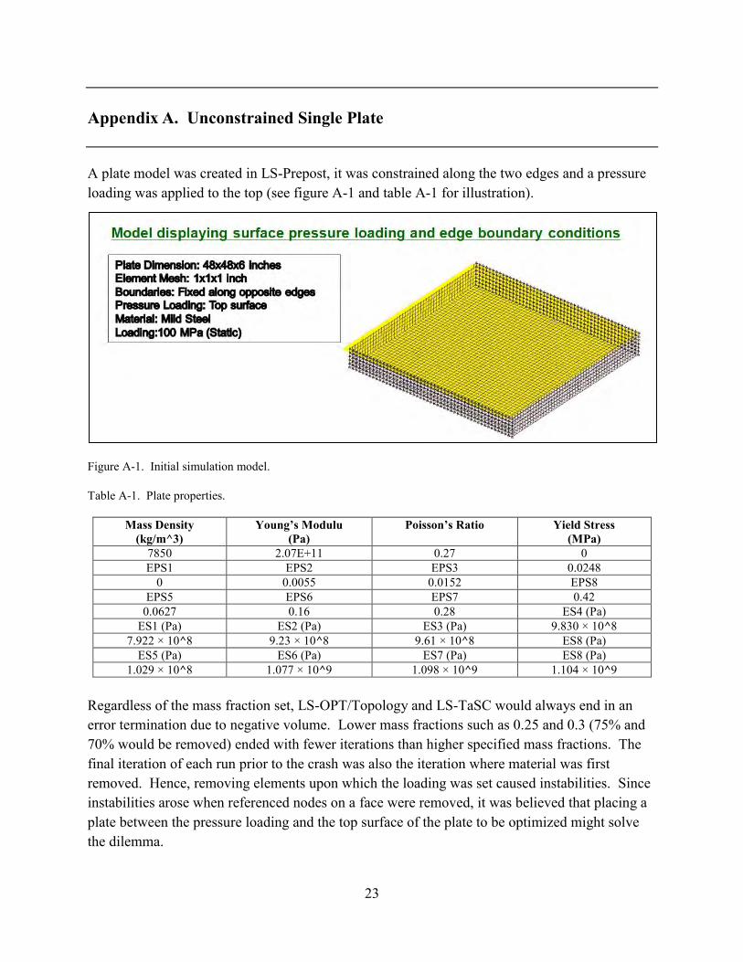
A plate model was created in LS-Prepost, it was constrained along the two edges and a pressure loading was applied to the top (see figure A-1 and table A-1 for illustration).

Figure A-1. Initial simulation model.

Table A-1. Plate properties.

Mass Density (kg/m^3)

Young’s Modulu (Pa)

Poisson’s Ratio Yield Stress (MPa)

7850 2.07E+11 0.27 0 EPS1 EPS2 EPS3 0.0248

0 0.0055 0.0152 EPS8 EPS5 EPS6 EPS7 0.42

0.0627 0.16 0.28 ES4 (Pa) ES1 (Pa) ES2 (Pa) ES3 (Pa) 9.830 × 10^8

7.922 × 10^8 9.23 × 10^8 9.61 × 10^8 ES8 (Pa) ES5 (Pa) ES6 (Pa) ES7 (Pa) ES8 (Pa)

1.029 × 10^8 1.077 × 10^9 1.098 × 10^9 1.104 × 10^9

Regardless of the mass fraction set, LS-OPT/Topology and LS-TaSC would always end in an error termination due to negative volume. Lower mass fractions such as 0.25 and 0.3 (75% and 70% would be removed) ended with fewer iterations than higher specified mass fractions. The final iteration of each run prior to the crash was also the iteration where material was first removed. Hence, removing elements upon which the loading was set caused instabilities. Since instabilities arose when referenced nodes on a face were removed, it was believed that placing a plate between the pressure loading and the top surface of the plate to be optimized might solve the dilemma.

24

INTENTIONALLY LEFT BLANK.

25

Appendix B. Constrained Single Plate with Top Pressure Plate (No Contact Defined)

The plates that are designed can only be allowed to deflect a certain distance. Hence, a deflection constraint would need to be set in LS-OPT/Topology. Fortunately, the release of the second version of LS-OPT/Topology (LS-TaSC) was promised to have a deflection constraint. We set the reference node to be in the center on the top of the top plate that was not to be optimized. The maximum deflection was set to be –0.25. The deflection of the plate before it was to be optimized was –0.1214. The only change made in LS-TaSC between the run with no constraints set (mirroring LS-OPT/Topology) and this run was that a deflection was set. A NODOUT was also set in the LS-Prepost model.

Upon running LS-TaSC with the only modification being the deflection constraint, it was immediately seen that within the first several iterations, LS-TaSC was optimizing the plate differently that it did the unconstrained plate. The unconstrained plate was optimized by having material removed from linear, parallel sections. LS-TaSC tried optimizing the plate with the deflection constraint by taking a big scoop out of the center from the top as can be seen in figures B-1 and B-2 (the top plate is hidden in these views). The run ended on the eleventh iteration with an error termination due to negative volume.

Figure B-1. LS-TaSC deflection constraint iteration 11.

26

Figure B-2. LS-TaSC deflection constraint optimization process.

Figures B-3 and B-4 show how the top plate goes down through the solid bottom plate on the 11th iteration.

Figure B-3. LS-TaSC deflection constraint instability.

27

Figure B-4. LS-TaSC deflection constraint optimization process instability.

28

INTENTIONALLY LEFT BLANK.

29

Appendix C. Constrained Single Plate with Top Pressure Plate (With Contacts Defined)

The model was then modified to have a CONTACT_AUTOMATIC_SINGLE_SURFACE with ssid set to 1, msid set to 2, sstyp set to 3, and mstyp set to 3. It was also decided to set SLDTHK=1 mm and “Mass scaling” DT2MS = (-)smallest_dt. These modifications had no influence on the optimization and the LS-TaSC continued to end on iteration 11 with the same instabilities that resulted with no contact defined. Figure C-1 shows the result.

Figure C-1. LS-TaSC deflection constraint optimization CONTACT_AUTOMATIC_SINGLE_SURFACE.

It was then decided to replace the CONTACT_AUTOMATIC_SINGLE_SURFACE with CONTACT_ERODING_SINGLE_SURFACE which also ended on iteration 11. However, in this run the instabilities allowed the top plate and the area of the bottom plate it traveled through to disappear, as can be seen in figure C-2.

30

Figure C-2. LS-TaSC deflection constraint optimization CONTACT_ERODING_SINGLE_SURFACE.

Since removal of elements from the top surface continued to be a source of problems for the optimization of this model, it was thought that setting a casting constraint from the bottom surface might be a solution. Although the CONTACT_AUTOMATIC_SINGLE_SURFACE did not prevent the instabilities in the model, it was believed that having one set was good practice and models used in following runs contained a CONTACT_AUTOMATIC_SINGLE_SURFACE.

31

NO. OF COPIES ORGANIZATION 1 ADMNSTR ELEC DEFNS TECHL INFO CTR ATTN DTIC OCP 8725 JOHN J KINGMAN RD STE 0944 FT BELVOIR VA 22060-6218 1 DARPA ATTN DEFENSE SCIENCE OFC S WAX 3701 N FAIRFAX DR ARLINGTON VA 22203-1714 1 DARPA ADVANCED TECH OFC ATTN D HONEY 3701 N FAIRFAX DR ARLINGTON VA 22203-1714 1 DARPA TACTICAL TECH OFC ATTN W JOHNSON 3701 N FAIRFAX DR ARLINGTON VA 22203-1714 1 DIR ATTN DTRA MSC 6201 8725 JOHN J KINGMAN RD FT BELVIOIR VA 22060-6201 1 PM COMBAT SYS ATTN SFAE GCS CS 6501 ELEVEN MILE MD WARREN MI 48397-5000 3 PM FCS (BCT) MSI ATTN SFAE GCS UA P CAG ATTN SFAE GCS UA S GRIEG ATTN SFAE GCS UA T MCKHEEN 6501 ELEVEN MILE RD WARREN MI 48397-5000 1 US ARMY RDECOM-TARDEC SURVIVABILITY LEAD MRAP JPO PEO-GROUND COMBAT SYS ATTN AMSTA TAR S D TEMPLETON 6501 E ELEVEN MILE RD WARREN MI 48397-5000

NO. OF COPIES ORGANIZATION 1 US ARMY TARDEC- SURVIVABILITY ATTN MS 2222 MAJ L ROSS 6501 E ELEVEN MILE RD BLDG 200C RM 1162 WARREN MI 48397-5000 1 US ARMY RDECOM-TARDEC SURVIVABILITY LEAD MRAP JPO PEO-GROUND COMBAT SYS ATTN SFAE GCS MRAP (MS 298) M CHAIT 6501 E ELEVEN MILE RD WARREN MI 48397-5000 1 US ARMY RDECOM-TARDEC SURVIVABILITY LEAD MRAP JPO PEO-GROUND COMBAT SYS ATTN SFAE GCS MRAP (MS 298) S KNOTT 6501 EAST ELEVEN MILE RD WARREN MI 48397-5000 1 US ARMY RDECOM-TARDEC SURVIVABILITY LEAD MRAP JPO PEO-GROUND COMBAT SYSTEMS ATTN SFAE GCS MRAP MS 298 R GOETZ 6501 E ELEVEN RD MS 263 WARREN MI 48397-5000 1 US ARMY RDECOM-TARDEC SURVIVABILITY LEAD MRAP JPO PEO-GROUND COMBAT SYS ATTN SFAE GCS MRAP (MS 298) E BARSHAW 6501 E ELEVEN MILE RD MS 211 WARREN MI 48397-5000 1 US ARMY ATCOM AVIATION APPLD TECHL DIR ATTN J SCHUCK FT EUSTIS VA 23604 1 US ARMY MATERIEL COMMAND ATTN AMSMI INT 9301 CHAPEK RD FT BELVOIR VA 22060-5527

32

NO. OF COPIES ORGANIZATION 1 US ARMY RDECOM ATTN AMSRD TAR R C FILAR 6501 E ELEVEN MILE RD MS 263 WARREN MI 48397-5000 1 US ARMY RDECOM ATTN AMSRD TAR R D DICEASURE 6501 E ELEVEN MILE RD WARREN MI 48397-5000 1 US ARMY RDECOM ATTN AMSRD TAR R D HANSEN 6501 E ELEVEN MILE RD MS 271 WARREN MI 48397-5000 1 US ARMY RDECOM ATTN AMSRD TAR R D OSTBERG 6501 E ELEVEN MILE RD MS 263 WARREN MI 48397-5000 1 US ARMY RDECOM ATTN AMSRD TAR R J BENNETT 6501 E ELEVEN MILE RD MS 271 WARREN MI 48397-5000 2 US ARMY RDECOM ATTN AMSRD TAR R L HINOJOSA ATTN AMSRD TAR R S HODGES 6501 E ELEVEN MILE RD MS 263 WARREN MI 48397-5000 1 DIRECTOR US ARMY RSRCH LAB ATTN RDRL ROE N B LAMATTINA PO BOX 12211 RESEARCH TRIANGLE PARK NC 27709-2211 1 US ARMY TACOM ATTN AMSRD TAR R/263 L FRANKS 6501 E 11 MILE RD WARREN MI 48397-5000 1 US ARMY TACOM PEO CS & CSS PM LIGHT TACTICAL VHCLS ATTN SFAE CSS LT M1114 MGR 6501 ELEVEN MILE RD WARREN MI 48397-5000

NO. OF COPIES ORGANIZATION 1 PM JLTV ATTN LTC PETERMAN 6501 E 11 MILE RD WARREN MI 48397-5000 1 PEO LAND SYSTEMS USMC ATTN PM JLTV LTC B GARZA 2200 LESTER ST BLDG 2208A QUANTICO VA 22134 1 PEO LAND SYSTEMS USMC DIRECTOR S&T ATTN M HALLORAN 2200 LESTER ST QUANTICO VA 22134 1 MARINE CORPS SYSTEMS CMD ATTN GTES TECHNOLOGIST W. SCOTT STORY 2200 LESTER ST BLDG 2208A QUANTICO VA 22134 1 MARINE CORPS ATTN J BURNS 2200 LESTER ST QUANTICO VA 22134 1 PEO LAND SYSTEMS ATTN PM JLTV US MARINE CORPS P MANTERNACH 2200 LESTER ST BLDG 2208A QUANTICO VA 22134 2 MARINE CRPS SCI & TECH OFC OF NVL RSRCH ATTN CODE 30 J BRADEL ATTN CODE 30 L MASTROIANNI 875 N RANDOLPH ST STE 1156B ONE LIBERTY CENTER ARLINGTON VA 22203-1995 1 NAV SURFC WARFARE CTR ATTN U SORATHIA 9500 MACARTHUR BLVD WEST BETHESDA MD 20817-5700 2 NAV SURFC WARFARE CTR CARDEROCK DIV ATTN CODE 28 R PETERSON ATTN CODE 6553 R CRANE 9500 MACARTHUR BLVD WEST BETHESDA MD 20817-5700

33

NO. OF COPIES ORGANIZATION 1 NSWC CARDEROCK DIV ATTN CODE 667 T BURTON 9500 MACARTHER BLVD WEST BETHESDA MD 20817-5700 1 LOS ALAMOS NATL LAB ATTN MS B216 F ADDESSIO PO BOX 1633 LOS ALAMOS NM 87545 1 CENTRAL INTLLGNC AGCY ATTN WINPAC/CWTG/GWET M DAN RM 4P07 NHB WASHINGTON DC 20505 2 BAE SYSTEMS ATTN R SCIORTINO ATTN T STEELE PO BOX 15512 YORK PA 17405-1512 1 DIR DEFENSE INTELLIGENCE AGENCY ATTN TA 5 K CRELLING WASHINGTON DC 20310 1 GEN DYNAMICS LAND SYS STERLING HEIGHTS COMPLEX ATTN T ZELEZNIK 38500 MOUND RD STERLING HEIGHTS MI 48310-3200 2 GENERAL DYNAMICS LAND SYSTEMS ATTN B CALDWELL ATTN G TEAL PO BOX 1800 WARREN MI 48090-1800 1 GLDS ATTN MZ436 21 24 J ERIDON 38500 MOUND RD STERLING HEIGHTS MI 48310-3200 2 THE BOEING CO ATTN J CHILDRESS ATTN N GERKEN MS 84-89 PO BOX 3707 SEATTLE WA 98124

NO. OF COPIES ORGANIZATION 1 UNITED DEFNS LIMITED PARTNERS ATTN J BRODY 4800 EAST RIVER RD MINNEAPOLIS MN 55421-1498 1 UNITED DEFNS LIMITED PARTNERS ATTN M242 W BALLATA 4800 E RIVER DR MINNEAPOLIS MN 55421-1498 1 UNITED DEFNS LIMITED PARTNERS ATTN R BRYNSVOLD 4800 EAST RIVER RD MINNEAPOLIS MN 55421-1498 6 UNITED DEFNS LIMITED PARTNERS SYS DIV ATTN D SCHADE ATTN G THOMAS ATTN M IWEN ATTN M MIDDIONE ATTN R MUSANTE ATTN T PIKE PO BOX 359 SANTA CLARA CA 95050 1 SHIP HULL MECH & ELEC S&T SIV OFFICE OF NAVAL RSRCH ATTN RGS BARSOUM 800 N QUINCY ONR334 ARLINGTON VA 22217-5660 2 US ARMY RESEARCH LABORATORY ATTN RDRL WMP D S HUG ATTN RDRL WMP D V HERNANDEZ ABERDEEN PROVING GROUND MD 21005 1 US ARMY RESEARCH LABORATORY ATTN RDRL LOA F M ADAMSON ABERDEEN PROVING GROUND MD 21005-5066

34

NO. OF COPIES ORGANIZATION 1 US ARMY RESEARCH LABORATORY ATTN RDRL WMM D S WALSH BLDG 4600 RM 2049 ABERDEEN PROVING GROUND MD 21005-5069 1 US ARMY RSRCH LAB ATTN RDRL SL R COATES BLDG 328 ABERDEEN PROVING GROUND MD 21005 2 US ARMY RSRCH LAB ATTN RDRL SLB A E HUNT ATTN RDRL SLB A J PLOSKONKA ABERDEEN PROVING GROUND MD 21005 1 US ARMY RSRCH LAB ATTN RDRL SLB E D LYNCH BLDG 328 ABERDEEN PROVING GROUND MD 21005 3 US ARMY RSRCH LAB ATTN RDRL WM (A) ATTN RDRL WM L BURTON ATTN RDRL WML G W DRYSDALE BLDG 4600 ABERDEEN PROVING GROUND MD 21005 4 US ARMY RSRCH LAB ATTN RDRL WML H B SORENSEN ATTN RDRL WML H E KENNEDY ATTN RDRL WML H L MAGNESS ATTN RDRL WML H T FARRAND BLDG 309 ABERDEEN PROVING GROUND MD 21005 1 US ARMY RSRCH LAB ATTN RDRL WML J NEWILL BLDG 390 ABERDEEN PROVING GROUND MD 21005 1 US ARMY RSRCH LAB ATTN RDRL WML M J ZOLTOSKI BLDG 4600 ABERDEEN PROVING GROUND MD 21005

NO. OF COPIES ORGANIZATION 3 US ARMY RSRCH LAB ATTN RDRL WMM A J SANDS ATTN RDRL WMM A J WOLBERT ATTN RDRL WMM A S GHIORSE ABERDEEN PROVING GROUND MD 21005 2 US ARMY RSRCH LAB ATTN RDRL WMM A S MCKNIGHT ATTN RDRL WMM B B CHEESEMAN BLDG 4600 ABERDEEN PROVING GROUND MD 21005 1 US ARMY RSRCH LAB ATTN RDRL WMM B C FOUNTZOULAS ABERDEEN PROVING GROUND MD 21005 3 US ARMY RSRCH LAB ATTN RDRL WMM B C YEN ATTN RDRL WMM B M VANLANDINGHAM ATTN RDRL WMMÊB R DOOLEY BLDG 4600 ABERDEEN PROVING GROUND MD 21005 1 US ARMY RSRCH LAB ATTN RDRL WMM B T BOGETTI ABERDEEN PROVING GROUND MD 21005 2 US ARMY RSRCH LAB ATTN RDRL WMM C R JENSEN ATTN RDRL WMM D E CHIN BLDG 4600 ABERDEEN PROVING GROUND MD 21005 7 US ARMY RSRCH LAB ATTN RDRL WMM E G A GILDE ATTN RDRL WMM E J LASALVIA ATTN RDRL WMM E P DEHMER ATTN RDRL WMM E P PATEL ATTN RDRL WMM F J MONTGOMERY ATTN RDRL WMM F K DOHERTY ATTN RDRL WMP A B RINGERS ABERDEEN PROVING GROUND MD 21005

35

NO. OF COPIES ORGANIZATION 1 US ARMY RSRCH LAB ATTN RDRL WMP B B LEAVY BLDG 393 ABERDEEN PROVING GROUND MD 21005 2 US ARMY RSRCH LAB ATTN RDRL WMP B C HOPPEL ATTN RDRL WMP B J CLAYTON BLDG 390 ABERDEEN PROVING GROUND MD 21005 1 US ARMY RSRCH LAB ATTN RDRL WMP C T W BJERKE BLDG 4600 ABERDEEN PROVING GROUND MD 21005 2 US ARMY RSRCH LAB ATTN RDRL WMP D B SCOTT ATTN RDRL WMP D D KLEPONIS ABERDEEN PROVING GROUND MD 21005 1 US ARMY RSRCH LAB ATTN RDRL WMP D J RUNYEON BLDG 393 ABERDEEN PROVING GROUND MD 21005 2 US ARMY RSRCH LAB ATTN RDRL WMP D M KEELE ATTN RDRL WMP D T HAVEL ABERDEEN PROVING GROUND MD 21005 1 US ARMY RSRCH LAB ATTN RDRL WMP E B LOVE BLDG 4600 ABERDEEN PROVING GROUND MD 21005 1 US ARMY RSRCH LAB ATTN RDRL WMP E D HACKBARTH ABERDEEN PROVING GROUND MD 21005

NO. OF COPIES ORGANIZATION 1 US ARMY RSRCH LAB ATTN RDRL WMP E E HORWATH BLDG 1100E ABERDEEN PROVING GROUND MD 21005 1 US ARMY RSRCH LAB ATTN RDRL WMP E M BURKINS BLDG 393 ABERDEEN PROVING GROUND MD 21005 2 US ARMY RSRCH LAB ATTN RDRL WMP E M KLUSEWITZ ATTN RDRL WMP E M LOVE ABERDEEN PROVING GROUND MD 21005 1 US ARMY RSRCH LAB ATTN RDRL WMP E W GOOCH BLDG 393 ABERDEEN PROVING GROUND MD 21005 1 US ARMY RSRCH LAB ATTN RDRL WMP F D FOX ABERDEEN PROVING GROUND MD 21005 1 US ARMY RSRCH LAB ATTN RDRL WMP F N GNIAZDOWSKI BLDG 390 ABERDEEN PROVING GROUND MD 21005 1 US ARMY RSRCH LAB ATTN RDRL WMP G N ELDREDGE BLDG 4600 ABERDEEN PROVING GROUND MD 21005 1 US ARMY RSRCH LAB ATTN RDRL WMP P J BAKER BLDG 309 ABERDEEN PROVING GROUND MD 21005

36

NO. OF COPIES ORGANIZATION 1 US ARMY RSRCH LAB ATTN RDRL WMP S E SCHOENFELD BLDG 393 ABERDEEN PROVING GROUND MD 21005 1 US ARMY RSRCH LAB ATTN RDRL WMP E C KRAUTHAUSER BLDG 1100E ABERDEEN PROVING GROUND MD 21005-5001 3 US ARMY RSRCH LAB ATTN RDRL VTA J A BORNSTEIN ATTN RDRL WMM A M MAHER ATTN RDRL WMM E J JESSEN ABERDEEN PROVING GROUND MD 21005-5066 2 US ARMY RSRCH LAB ATTN RDRL WMP F R BITTING ATTN RDRL WMP F R GUPTA BLDG 309 ABERDEEN PROVING GROUND MD 21005-5066 1 US ARMY RSRCH LAB ATTN RDRL WMP F X HUANG ABERDEEN PROVING GROUND MD 21005-5066 1 US ARMY RSRCH LAB ATTN RDRL WMP G S KUKUCK BLDG 309 ABERDEEN PROVING GROUND MD 21005-5066 2 US ARMY RSRCH LAB ATTN RDRL SLB A B WARD ATTN RDRL SLB A P KUSS ABERDEEN PROVING GROUND MD 21005-5068 2 US ARMY RSRCH LAB ATTN RDRL SLB D J POLESNE ATTN RDRL SLB D R GROTE BLDG 1068 ABERDEEN PROVING GROUND MD 21005-5068

NO. OF COPIES ORGANIZATION 1 US ARMY RSRCH LAB ATTN RDRL WMP F E FIORAVANTE BLDG 309 ABERDEEN PROVING GROUND MD 21010-5423 1 US ARMY RSRCH LABORATORY ATTN RDRL WMM E J CAMPBELL BLDG 4600 ABERDEEN PROVING GROUND MD 21005 1 US ARMY RSRCH OFC ATTN RDRL ROE M D STEPP PO BOX 12211 RESEARCH TRIANGLE PARK NC 27709-2211 1 US ARMY TACOM ATTN AMSTA CS CI F SCHWARZ 6501 E ELEVEN MILE RD MS 105 WARREN MI 48397-5000 5 US ARMY RSRCH LAB ATTN IMNE ALC HRR MAIL & RECORDS MGMT ATTN RDRL CIO LL TECHL LIB ATTN RDRL CIO MT TECHL PUB ATTN RDRL DP R R SKAGGS ATTN RDRL WMP F A FRYDMAN ADELPHI MD 20783-1197