Constraining modi ed gravity with quantum optomechanics

Constraining modified gravity with quantum optomechanics

Sofia Qvarfort1,2, Dennis Ratzel3, Stephen Stopyra2

1 QOLS, Blackett Laboratory, Imperial College London, SW7 2AZ London, United Kingdom2 Department of Physics and Astronomy, University College London, Gower Street, WC1E 6BT London,United Kingdom3 Institut fur Physik, Humboldt-Universitat zu Berlin, 12489 Berlin, Germany

E-mail: [email protected], [email protected]

Abstract. We derive the best possible bounds that can be placed on Yukawa– and chameleon–likemodifications to the Newtonian gravitational potential with a cavity optomechanical quantum sensor. Bymodelling the effects on an oscillating source-sphere on the optomechanical system from first-principles,we derive the fundamental sensitivity with which these modifications can be detected in the absence ofenvironmental noise. In particular, we take into account the large size of the optomechanical probe comparedwith the range of the fifth forces that we wish to probe and quantify the resulting screening effect when boththe source and probe are spherical. Our results show that optomechanical systems in high vacuum could,in principle, further constrain the parameters of chameleon-like modifications to Newtonian gravity.

arX

iv:2

108.

0074

2v1

[qu

ant-

ph]

2 A

ug 2

021

Constraining modified gravity with quantum optomechanics 2

1. Introduction

General Relativity is one of the most successful theories of nature, but there are compelling reasons toexplore modifications to the behaviour of gravity on both large and small scales. Most of the precisepredictions of General Relativity have consistently been demonstrated experimentally: among many othersthese include the perihelion shift of Mercury [1] and the existence of gravitational waves [2]. Similarly,the current standard cosmological model, the Λ Cold Dark Matter (ΛCDM) model, is another of GeneralRelativity’s success stories. However, in order to match observation, ΛCDM requires a positive cosmologicalconstant [3, 4]. This is backed up by observations of supernovae, which indicate that the Universe’s expansionis accelerating [5]. While a natural part of General Relativity, a cosmological constant poses a theoreticalchallenge to particle physics since the small observed value is inherently sensitive to high-energies, requiringdelicate balancing [6]. Furthermore, many theories of high energy physics that attempt to solve this andother problems – such as building a consistent quantum theory of gravity – predict deviations from GeneralRelativity. These theories are collectively known as modified gravity theories.

Modified gravity theories, however, typically face a difficult challenge in the form of solar system testsof Newton’s laws. Models that differ from General Relativity significantly enough to explain the observedacceleration of the Universe on large scales are typically ruled out by their predicted deviations on smallerscales (solar system and laboratory tests) [7–9]. There are a large variety of approaches to modified gravity– see Koyama [10] for a comprehensive review – but many models attempt to address the problem of solarsystem tests via a screening mechanism [11]. Such mechanisms can be built into modified gravity theoriesto conceal deviations on solar system scales, without changing the large scale behaviour. An approachconsidered by many authors is the chameleon mechanism [12–14]; the basic idea is to add a scalar field thatcouples directly to gravity in a manner that depends on the local density of matter. In high-density regions,such as inside a galaxy, the effects of modified gravity are screened out, allowing the theory to evade solarsystem tests. In the low-density void regions between galaxies, however, the effects of modified gravity wouldbe unscreened.

If such a density-dependent gravity mechanism is at play, it ought to be detectable in principle byhigh-precision laboratory experiments. In particular, the fundamental sensitivity improvements offered byquantum systems are especially promising [15]. At the moment, the detection of modified gravity, andin particular, chameleon fields, has been explored through a diverse variety of methods. Searches withclassical systems include theoretical proposals for torsion balance tests of fifth forces [16–22], some of whichhave already been carried out as experiments [23, 24]. Additional proposals suggest that experimentswhich measure Casimir forces may also be used to constrain chameleon theories [18, 25–28]. In atominterferometry, which is already routinely used for quantum sensing, the uniformity of the atoms as wellas the additional sensitivity gained from the superposition of flight-paths has led to impressive precisiongravimetry sensitivities [29–32]. Several proposals have explored in depth the possibilities of searching formodified gravity and dark energy with atom interferometry [33–39], and some of the most stringent boundson existing theories have been obtained in this way [40, 41]. Further viable routes towards detecting modifiedgravity include ultra-cold neutron experiments [42–48] and neutron interferometry [46, 49–52]. Finally, testsof atomic transition frequencies [53, 54], close examination of vacuum chambers and photo-detectors [55, 56],as well as tests of the electron magnetic moment [57] have also been proposed.

An additional approach to detecting the small-scale effects of modified gravity and screening is to takeadvantage of recent developments in the field of optomechanics, where a small mechanical element is coupledto a laser through radiation-pressure [58, 59]. Optomechanical system encompass a diverse set of platformswhich range from microscopic movable mirrors as part of a Fabry–Perot cavity [60], levitated particles [61],clamped membranes [62], liquid Helium [63] and trapped cold atoms [64]. When the mechanical elementis cooled down to sufficiently low temperatures, it enters into a quantum state that can be manipulatedthrough measurements and optical control techniques. Ground-state cooling has been demonstrated acrossa number of platforms, including clamped membranes [65, 66] and recently also for levitated systems [67].Optomechanical systems show promising potential as both classical and quantum-limited sensors [68–70],and recent studies have proposed their use as gravity sensors [71–74]. In fact, experimental searches forfifth forces with classical optomechanical setups have already been performed (see e.g. [75, 76]), where thebounds achieved fell within those excluded by atom interferometry. A key question, which we explore in thiswork, therefore becomes whether an optomechanical sensor in the quantum regime can improve on these


Vacuum chamber

Piezo

Figure 1. A gold source mass attached to a shear piezo oscillates to create a time-varying gravitational field.The field, which potentially contains deviations from Newtonian gravity, is detected by an optomechanicalprobe system where the photon number a†a couples to the mechanical position xm as a†axm, here presentedas a moving-end mirror in a Fabry–Perot cavity. The amplitude ε of the source mass oscillation is a fractionof the total distance r0 between the systems. By accounting for the vacuum background density, we mayalso compute bounds on the parameters of the chameleon screening mechanism.

bounds. For an overview of searches for new physics with levitated optomechanical systems, see the recentreview by Moore et al. [77]. The advantage of optomechanical sensors, as opposed to, for example, cold atominterferometry is that the sensitivity of the system can be improved while retaining the compact setup ofthe experiment. In contrast, improving the sensitivity of atom interferometry primarily relies on increasingthe length of the flight-path of the atoms.

The key question we seek to answer in this work is: what range of parameters of modified gravity theoriescan be excluded with an quantum optomechanical sensor? To address this question, we consider a systemdescribed by a fully-nonlinear, dispersive, optomechanical Hamiltonian‡ in the absence of environmentalnoise and decoherence. We then consider the gravitational field that arises when a source mass is placednext to the sensor. Since it is often difficult in experiments to distinguish a signal against a constant noisefloor, we consider an oscillating source mass, which gives rise to a time-dependent gravitational field. Sucha signal can then be isolated from other common low-frequency 1/f noise sources via a Fourier analysis ofthe data. To determine whether our analysis is valid in the case of a chameleon field, we derive the resultingtime-dependent potential from first principles, where we find that a potential that moves with the mass isthe correct choice for non-relativistic velocities. Another key consideration for optomechanical systems isthe relatively large size of the optomechanical probe, which we find contributes to the chameleon screeningof the fifth force (as opposed to, for example, cold atoms, where the screening length of the atomic probesis very small). To take the finite screening length into account, we go beyond the common approximationthat the probe radius is small compared to the range of the chameleon field and derive analytic expressionsfor the modified force seen by the probe. Then, using tools from quantum information theory and quantummetrology such as the quantum Fisher information, we are able to estimate the fundamental sensitivity fordetecting deviations from Newtonian gravity. To further improve the sensitivity, we also consider knownways to enhance the optomechanical sensor in the form of squeezed light and a modulated optomechanicalcoupling [74].

Our main results include the bounds presented in Fig. 3, which shows the parameter ranges of modifiedgravity theories that could potentially be excluded with an ideal optomechanical sensor. The bounds are

‡ This Hamiltonian is often linearised for a strong coherent input drive, however the fully nonlinear (in the sense of the equationsof motion) Hamiltonian is a more fundamental description. In this sense, our analysis specifically focuses on describing theintra-cavity state rather than the output.


computed for a specific set of experimental parameters. To facilitate investigations into additional parameterregimes, we have made the code used to compute the bounds available (see the Data Availability Statement).While experiments are unlikely to achieve the predicted sensitivities due to noise and systematic effects, ourbounds constitute a fundamental limit for excluding effects beyond Newtonian gravity given the experimentalparameters in question.

This work is structured as follows. In Section 2 we present the proposed experimental setup andoptomechanical Hamiltonian, and then we proceed to discuss Yukawa potentials as a modification to theNewtonian gravitational potential in Section 3. We consider those sourced by a chameleon field and providea first-principles’ derivation of the time-dependent potential that results from the mass oscillating aroundan equilibrium position. We also discuss screening effects inherent to chameleon fields and derive thescreening effect that arises from the size of the optomechanical probe. In Section 4, we linearise the modifiedgravitational potential, and in Section 5, we provide an introduction to quantum metrology and the quantumFisher information. These tools allows us to present analytic expressions for the fundamental sensitivity ofthe system, which we do in Section 6. The work is concluded by a discussion in Section 7 and some finalremarks in Section 8.

2. Experimental setup and optomechanical dynamics

We envision an experimental setup similar to that used in [78], where an oscillating source mass made ofsolid gold is placed in a vacuum chamber adjacent to an optomechanical probe (see Fig. 1). We have chosengold because we require the highest possible density in order to detect gravitational effects and maximisethe effect of density-dependent screening mechanisms such as chameleon fields§. The source mass oscillatesback and forth with the help of a shear piezo at a fixed frequency. The optomechanical probe is then allowedto move along the same axis as the oscillating mass. By injecting light into the cavity, the position of theoptomechanical coupling is dispersively coupled to the optical field through radiation-pressure. The strengthof the coupling between the optical and mechanical modes is different for each implementation, but theinteraction can generally be described through similar dynamics. In this work, we begin with a generaldescription, but later specialise towards a spherical system since it allows for analytical treatments of somemodified gravity potentials.

The optomechanical Hamiltonian, which governs the dynamics of the optomechanical probe, is given by(in the absence of an external gravitational field):

H0 = ~ωc Na + ~ωm Nb − ~ k(t) Na(b† + b

), (1)

where ωc and ωm are the oscillation frequencies of the optical cavity mode and mechanical mode respectively,with annihilation and creation operators a, a† and b, b†. We have also defined Na = a†a and Nb = b†b as thephoton and phonon number operators.

The coupling k(t) is the (potentially time-dependent) characteristic single-photon interaction strengthbetween the number of photons and the position of the mechanical element. It takes on different formsdepending on the optomechanical platform in question. Among the simplest couplings is that for a movingmirror that makes up one end of a cavity, k = (ωl/L)

√~/(2mωm), where ωl is the laser frequency and L is the

length of the cavity. In this work, we also consider modulating the coupling in time; it has been previouslyfound that such modulations can be used to enhance the sensitivity of the optomechanical sensor if theycan be made to match the oscillation of the external force [74]. Modulation of the optomechanical couplingcan be introduced in different ways depending on the experimental platform in question. For example, themechanical frequency of a cantilever can be modified by applying an oscillating electric field [79, 80], anda modulated coupling arises naturally through the micro-motion of a levitated system in a hybrid electro-optical trap [81–83].

When treating the system in a closed and ideal setting, we can model the initial state as a separable stateof the light and the mechanical element. For the optical state, we consider injecting squeezed light into thecavity. Squeezed light has been shown to fundamentally enhance the sensitivity to displacements [15]. The

§ While there are denser materials, such as depleted Uranium, gold is a stable material that has previously been used forsmall-mass sensing, see e.g. Ref [78].


state of the mechanical element, on the other hand, is most accurately described as thermal at a non-zerotemperature. With these assumptions, the initial state of the system can be written as

%(0) = |ζ〉〈ζ| ⊗∞∑n=0

tanh2n rT

cosh2 rT|n〉〈n| , (2)

where |ζ〉 = Sζ |µc〉 is a squeezed coherent state of the optical field where Sζ = exp[(ζ∗a2 − ζa†2)/2

]and

where the coherent state satisfies a |µc〉 = µc |µc〉. The squeezing parameter can also be in spherical polarform as ζ = r eiϕ. Squeezed states can be generated through four-wave mixing in an optical cavity [84] orparametric down-conversion [85]. See also Ref [86] for a review of squeezed state generation. The parameter

rT of the thermal state arises from the Bose–Einstein distribution and is defined by tanh rT = exp[− ~ωm

2 kB T

],

where T is the temperature of the system and kB is Boltzmann’s constant.In order to compute the sensitivity bounds for detecting modified gravity, we model the effect of the

gravitational force on the optomechanical system as a contribution to the dynamics. When the force isweak, it can be linearised and included as a displacement term in the optomechanical Hamiltonian shownin Eq. (1). In this section, we provide a general derivation of this linearised force, while in Section 4 wespecialise to Yukawa-like modifications to the Newtonian potential, as well as a chameleon modification.

We start by assuming that the source mass and the mechanical element of the optomechanical systemare constrained to move along the x-axis. We let the mechanical element be subject to a harmonic potentialcentered at x = 0 and we label the position of the source mass xS(t). Then, we assume that there is a smallperturbation to the centre-of-mass position of the mechanical element that we call δx, and, assuming that|xS(t)| |δx| at all times, we write the relative distance between the systems as xS(t)− δx. Provided thatδx remains small, we can Taylor expand the system to first order in δx. Given a generic potential termV (xS(t)− δx), we find, to first order in δx:

V (xS(t)− δx) = V (xS(t))− V ′(xS(t)) δx+O[(δx)2]. (3)

The first term in Eq. (3) represents a time-dependent shift of the overall energy, however it does notdepend on the position of the optomechanical system. The second term describes the (potentially time-dependent) displacement of the mechanical element with δx. The second-order term in δx leads to a shiftin the mechanical frequency that we do not model here, but dynamics of this kind have been previouslystudied [87]. The expansion in Eq. (3) is valid as long as δx remains small such that the higher-order termscan be neglected. We outline the conditions for this being true in the Discussion (see Section 7).

We proceed to promote δx to an operator δx→ xm, which can be written in terms of the annihilationand creation operators b and b† of the mechanical element as

xm = x0

(b† + b

), (4)

where x0 =√

~/(2mωm) is the zero-point fluctuation of the mechanical oscillator. The full optomechanicalHamiltonian including the modified gravitational potential can then be written as

H(t) = H0 − V ′(xS(t))x0

(b† + b

), (5)

where H0 is given in Eq. (1) and where the time-dependent modified Newtonian gravitational force iscontained in the second term G(t).

The time-evolution of the system with the Hamiltonian in Eq. (5) can be written as the followingtime-ordered exponential:

U(t) =←−T exp

[− i~

∫ t

0

dt′ H(t′)

], (6)

where the time-dependence of the gravitational potential in H(t) requires careful consideration. Suchdynamics have been studied previously [87, 88] and provide a short overview of the treatment Appendix C.Later on in this work, we use the expression for U(t) to derive the sensitivity of the system to modificationsof the Newtonian potential, but first, we will study the form of the modifications in-depth.


3. Modified gravitational potential and screening from the source and the probe

In this section, we discuss an example of how the chameleon mechanism would alter the Newtonian force lawon sub-millimetre scales. We write all equations in terms of SI units, but energy units (as used elsewhere inthe literature) can be restored by setting ~ = c = 1 throughout.

3.1. Yukawa modifications to the gravitational force law

Although there are many ways of modifying Newton’s laws on short distances, perhaps one of the bestmotivated theoretically is to add a Yukawa term to the potential. Yukawa potentials are ubiquitous inscalar field theories, since they are the solution to the sourced (inhomogeneous) Klein–Gordon equation for amassive field in the case of spherical symmetry. As a consequence of Lovelock’s theorem [89], modifications toGeneral Relativity require either additional degrees of freedom such as a scalar field, or more exotic scenariossuch as large extra dimensions, higher derivatives, or non-locality. Consequently, additional scalar fields arecommon in modified gravity theories. These act like a fifth force and give rise to a gravitational potential ofthe form:

V (r) = −GMSm

r

(1 + α e−r/λ

), (7)

where α parametrises the intrinsic difference in strength between the Yukawa-like fifth force and gravity,while λ parametrises the range of this fifth-force. Note that it is possible to have α 1 and still agree withexisting constraints, provided the force is sufficiently short range to have evaded tests of gravity on shortdistances.

For this work, we will consider a chameleon screening mechanism that gives rise to a Yukawa-like force.However, the methods we describe can be broadly applied to many different Yukawa-type modifications ofthe gravitational field on short distances. In the chameleon mechanism, short distance modifications to theNewtonian force law are screened from the reach of solar system tests by the presence of a density-dependentscalar field, known as the chameleon field. In regions of relatively high average density – such as can befound inside a galaxy – the chameleon field has a high mass, making it hard to detect at colliders andaltering the gravitational force law in such a way as to be consistent with solar-system experiments (this isthe ‘screening’ effect). However, in regions of low-density – such as in cosmological voids – the field is lighterand the effects of modified gravity unscreened. This allows modified gravity theories to have substantialeffects on cosmological scales, while being difficult to detect on galactic or solar-system scales.

We review the properties of chameleon fields in Appendix A. The net effect of the chameleon scalar fieldis to modify the effective Newtonian potential affecting a test particle. Specifically, the effective potential atposition x is given by

Φeff(x) = ΦN (x) + ΦC(x) ≈ ΦN (x) +φ(x)

M, (8)

where ΦN is the standard Newtonian potential, and ΦC is the modification to it arising from the chameleonfield. The parameter M (here chosen to be a mass to give the correct units for a potential) determines howstrongly the chameleon field affects test particles and arises from the non-minimal coupling of the chameleonfield to curvature as discussed in Appendix A.

In this work, we consider a chameleon model with an effective interaction potential

Veff(φ) =Λ4+n

φn+φρ

M(~c)3. (9)

We explore only the case n = 1 in this work: other models and choices of n are possible, but we choose thisspecific example to demonstrate how the method works in principle. This model has two parameters; Λ,which characterises the energy scale of the chameleon’s self-interaction potential; and M which characteriseshow strongly the chameleon responds to the local mass density, ρ.

For n = 1 the background value of the field, φbg, in an environment of constant mass density ρbg isgiven by

φbg =

√MΛ5

ρbg(~c)3. (10)


In the centre of the source, the chameleon field reaches its minimum value of φS (which can be obtained byreplacing the density ρbg in Eq. (10) with the source density ρS). The mass of the chameleon field, mbg, isdensity dependent (see Appendix A) and given by

mbgc2 =

(4 ρ3

bg(~c)9

M3Λ5

)1/4

. (11)

The key question for us is how the field results in a force on the optomechanical sensor. This is what weconsider next.

3.2. Force on the optomechanical sensor

The effect of a chameleon field is in principle detectable in a high-vacuum environment. In practise, thisrequires extremely precise acceleration measurements, which an optomechanical system can provide. In thiswork we will model both the source mass and the detector probe as spheres, and compute the sensitivityusing the Chameleon force between these two spheres. There are therefore two effects to consider: theresponse of the field in Eq. (8) to the spherical source, and the response of the probe to that field. Due tothe nature of the chameleon field, a non-point-like probe will not simply follow the gradient of Eq. (8) aswould a test particle: instead there is an additional screening effect due to the interactions of the probe itselfwith the field.

To derive the force that acts on the sensor, we consider the field inside the vacuum chamber. Burrageet al. [33] derived the chameleon field around a spherical source of mass MS and radius RS as a function ofdistance from the centre of the sphere, r. They assumed in their derivation that the range of the chameleonforce was large compared to the size of the source (that is, mbgRSc/~ 1). To allow us to consider a broadparameter space, we do not assume that either mbgRSc/~ 1 or mbgRP c/~ 1 where the indices S andP denote the source and probe, respectively. In what follows, we go beyond existing studies in this regardby including sources (probes) with non-negligible size compared to the range of the force.

We use the same asymptotic matching approach as Burrage et al. [33] to obtain an expression for thechameleon field around a spherical matter distribution:

φ(r) =

φi, r < Si

φS + ~cMS

8πRiMr3−3S2

i r+2S3i

rR2i

, Si < r < Ri

φbg − ~cMi

4πrM(1+mbgRic/~)

(1− S3

i

R3i

)e−mbgc(r−Ri)/~, r > RS

. (12)

Here, i = S, P for the source and probe respectively. φi is the equilibrium value of the chameleon field in amaterial with the source (probe) density: the field will attain this value at some radius Si ≤ Ri. There is thena transition layer where the field φi increases to its surface value, before increasing to the equilibrium value inthe background density, φbg. The range of the force outside the source is controlled by the density-dependentchameleon mass, mbg. The full derivation of Eq. (12) is given in Appendix A.1.

The value of the length scale Si depends on the source/probe properties, the chameleon model, andenvironmental properties. For the model we consider here, it is found by solving the following cubic equation:

S2i

R2i

+2

3

[1

1 +mbgRic/~− 1

]S3i

R3i

= 1− 8πM

3MiRi(φbg − φi)c/~ +

2

3

[1

1 +mbgRic/~− 1

]. (13)

In the mbgRic/~→ 0 and φbg φi limits, this reduces to

Si = RS

√1− 8πM

3Mi

Riφbg

~c, (14)

which is the result found by Burrage et al. [33]. Si parametrises the screening effect of the chameleonmechanism for a spherical source/probe: for example, when Si is much lower than Ri, the field is effectivelyunscreened while for Si ≈ Ri the field is heavily screened. Outside of the source (r > Ri), we see fromEq. (12) that the scalar field, and thus the modified gravitational potential, has an effective Yukawa form.


Thus, a chameleon field of this type would manifest as a Yukawa-like modification to the acceleration ofa test particle. Since our proposed experimental setup will involve measuring acceleration outside of thesphere, we only need the r > Ri part of the solution.

When viewed as a Yukawa-type force of the form considered in Eq. (7), and when the probe itself doesnot contribute to the screening, the resulting fifth-force strength α and range λ are given by

αbg =2M2

P

M2ξS , and λbg =

~mbgc

, (15)

where MP ≈√~c/(8πG) = 4.341 × 10−9 kg is the reduced Planck mass (here expressed as a mass rather

than an energy), αbg depends on the background density through ξS , which is given by [33]

ξS =

1, ρSR

2S < 3M φbg/(~c),

1− S3S

R3S, ρSR

2S > 3Mφbg/(~c) .

(16)

As long as the optomechanical sensor is approximated as a point-particle, such that RP /λbg 1, the forcefelt by the optomechanical probe can therefore be written as

F = −GMSm

|xS |2

[1 + αbg

(1 +|xS(t)|λbg

)e−|xS(t)|/λbg

]. (17)

The point-particle approximation is however quite severe, especially for an optomechanical probe, the radiusof which can be quite large compared with the range of the force in question. We proceed to consider thescreening from the probe in the following section.

3.3. Chameleon screening from the optomechanical probe

Compared with the atoms used in alternative approaches to the detection of fifth-force modifications togravity, such as atom interferometry, the optomechanical probe can potentially be relatively large comparedto the range of fifth forces. This can result in significant contributions to the chameleon field screening.The screening depends strongly on the geometry of the system; in general, numerical methods are needed tocompute the full screening [90]. As such, it is difficult to estimate the screening for say a Fabry–Perot moving-end mirror; however the problem is simplified when both the source sphere and the probe are sphericallysymmetric. This is the case when the mechanical element in the optomechanical system is a levitated sphere,made, for example, by silica.

To estimate the extent of the screening for a spherical optomechanical probe, we consider the force thatarises from the movement on the time-dependent mass. See Appendix B.3 for the full calculation. In thelimit where the probe radius is much smaller than the distance between the probe and the source sphereRP |xS(t)|, we find the following expression for the force:

F = −GMSm

|xS |2

[1 + αbg,P

(1 +|xS(t)|λbg

)e−|xS(t)|/λbgf(RP /λbg, |xS(t)|/λbg)

], (18)

where the sensor-dependent fifth-force strength is defined as

αbg,P =2M2

P

M2ξS ξP , (19)

where we have added the subscript ’P ’ to denote that screening from the probe is here taken into account.Furthermore, ξS and ξP (again labelled S for the source and P probe, respectively), are given in Eq. (16).To compute ξP , we replace MS , RS and ρS with MP , RP and ρP . Finally, the function f is a form-factorgiven by

f(x, y) = (1 + x) e−x[

sinh(x)

x−(

y

1 + y− 2

)1

y

(cosh(x)− sinh(x)

x

)]. (20)


This approaches 1 in the x = mbgRP c/~ = RP /λbg → 0 limit, in which case Eq. (18) reduces to the resultof Burrage et al. [33] for the force between two spheres. Since spherical probes or source masses generallymaximise the screening [90], Eq. (18) can be interpreted as a conservative estimate of the screening due tothe shielding from the probe.

Burrage et al. [33] make use of the RP /λbg → 0, since the probe radius in the case of atom interferometryis typically much smaller than λbg. For an optomechanical probe, however, the additional screeningintroduced by the probe can be substantial, but not, as we shall see, detrimental. In what follows, wecompute the sensitivity both with and without the screening from the probe, where the latter correspondsto approximating the probe as a point particle.

3.4. Potential from a moving source-mass

In this work, we consider a moving source mass. This brings up a consideration of how the chameleon fieldresponds to the motion of the source mass. For the gravitational field, we know that changes in the potentialpropagate outwards at the speed of light, and thus the appropriate potential to use is the retarded Newtonianpotential. The situation is less clear for the scalar field, however. Since it is massive, it is not immediatelyobvious information will propagate outwards at the speed of light. To get an idea of its behaviour we needto know the speed, vI , at which information propagates through the scalar field. We show in Appendix B.2that this is also, in fact, the speed of light. Consequently, the potential can be approximated by the timedependent form

ΦC(x, t) =φbg

M− GMS

|x− xS(t)|αbg e

−|x−xS(t)|/λbg . (21)

where t should be replaced with the retarded time given by Eq. (B.9), however, we can ignore this forthe non-relativistic speeds and distances considered in this setup. Since both the chameleon field, φ, andthe metric, gµν (which gives rise to the Newtonian potential, ΦN ) are well-defined dynamical quantities, thetime-dependence of this potential is well-defined. We note at this point that if quantum corrections are large,the effective speed of information propagation for the scalar field, vI , may differ from c [91]. However, largequantum corrections of this size would mean that we cannot readily use the effective field theory treatmentof the chameleon field assumed throughout [92], so we do not consider this effect here. We can therefore useEq. (21) in the discussion that follows to measure the values of α and λ, and thus the parameters Λ and Mof the chameleon field.

4. Linearised modified Newtonian potential

In order to compute the sensitivity of the optomechanical system, we need to include the force on the sensorshown in Eq. (18) into the dynamics of the optomechanical system. It is possible to obtain the solutionnumerically, but in order to obtain analytic expressions, we choose to linearise the Yukawa modification ofthe force for small oscillations of the source-mass. We let the time-dependent distance between the systemsxS(t) be given by:

xS(t) = r0 (1− ε cos(ω0 t+ φ0)) , (22)

where ε is a dimensionless oscillation amplitude defined as a fraction of r0, where ω0 is the oscillationfrequency and φ0 is a phase shift that we specify later in order to maximize the sensitivity.

In the following two sections, we show the linearisation of the force for a generic Yukawa potential, andfor the chameleon force with a large optomechanical probe that contributes to the screening.

4.1. Linearising the Yukawa potential

We now linearise the contributions from the Yukawa potential to Eq. (7) for small oscillation amplitudesε 1. We note that, for specific values of α and λ, higher order contributions to the Newtonian gravitationalforce may be larger than the first-order contributions to the Yukawa force. It is therefore important that,when taking data in an experiment, we determine the origin of the observed values (see the Discussion in


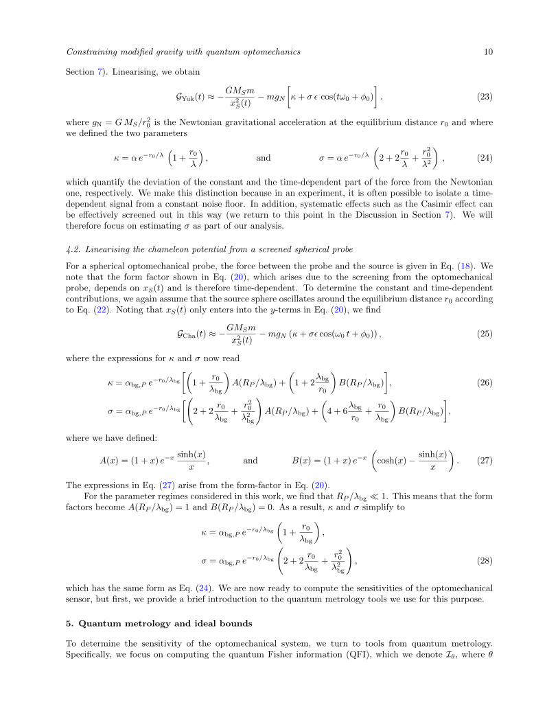
Section 7). Linearising, we obtain

GYuk(t) ≈ −GMSm

x2S(t)

−mgN[κ+ σ ε cos(tω0 + φ0)

]. (23)

where gN = GMS/r20 is the Newtonian gravitational acceleration at the equilibrium distance r0 and where

we defined the two parameters

κ = α e−r0/λ(

1 +r0

λ

), and σ = α e−r0/λ

(2 + 2

r0

λ+r20

λ2

), (24)

which quantify the deviation of the constant and the time-dependent part of the force from the Newtonianone, respectively. We make this distinction because in an experiment, it is often possible to isolate a time-dependent signal from a constant noise floor. In addition, systematic effects such as the Casimir effect canbe effectively screened out in this way (we return to this point in the Discussion in Section 7). We willtherefore focus on estimating σ as part of our analysis.

4.2. Linearising the chameleon potential from a screened spherical probe

For a spherical optomechanical probe, the force between the probe and the source is given in Eq. (18). Wenote that the form factor shown in Eq. (20), which arises due to the screening from the optomechanicalprobe, depends on xS(t) and is therefore time-dependent. To determine the constant and time-dependentcontributions, we again assume that the source sphere oscillates around the equilibrium distance r0 accordingto Eq. (22). Noting that xS(t) only enters into the y-terms in Eq. (20), we find

GCha(t) ≈ −GMSm

x2S(t)

−mgN (κ+ σε cos(ω0 t+ φ0)) , (25)

where the expressions for κ and σ now read

κ = αbg,P e−r0/λbg

[(1 +

r0

λbg

)A(RP /λbg) +

(1 + 2

λbg

r0

)B(RP /λbg)

], (26)

σ = αbg,P e−r0/λbg

[(2 + 2

r0

λbg+

r20

λ2bg

)A(RP /λbg) +

(4 + 6

λbg

r0+

r0

λbg

)B(RP /λbg)

],

where we have defined:

A(x) = (1 + x) e−xsinh(x)

x, and B(x) = (1 + x) e−x

(cosh(x)− sinh(x)

x

). (27)

The expressions in Eq. (27) arise from the form-factor in Eq. (20).For the parameter regimes considered in this work, we find that RP /λbg 1. This means that the form

factors become A(RP /λbg) = 1 and B(RP /λbg) = 0. As a result, κ and σ simplify to

κ = αbg,P e−r0/λbg

(1 +

r0

λbg

),

σ = αbg,P e−r0/λbg

(2 + 2

r0

λbg+

r20

λ2bg

), (28)

which has the same form as Eq. (24). We are now ready to compute the sensitivities of the optomechanicalsensor, but first, we provide a brief introduction to the quantum metrology tools we use for this purpose.

5. Quantum metrology and ideal bounds

To determine the sensitivity of the optomechanical system, we turn to tools from quantum metrology.Specifically, we focus on computing the quantum Fisher information (QFI), which we denote Iθ, where θ


is the parameter that we wish to estimate. Intuitively the QFI can be seen as a measure of how much thequantum state of the system changes given a specific encoding of θ. The QFI then provides a measure ofthe change in the state with θ compared with the case when the state is unaffected. See also Ref [93] for anintuitive introduction to the QFI and related concepts in quantum metrology.

The connection to sensitivity stems from the fact that the QFI provides a lower bound to the varianceVar(θ) of θ through the quantum Cramer–Rao bound [94, 95]:

Var(θ) ≥ 1

MIθ, (29)

whereM is the number of measurements or probes used in parallel. The standard deviation of θ is then givenby ∆θ = 1/

√MIθ. However, it is important to note that the QFI does not reveal the actual measurement

that yields the best sensitivity. To obtain this information, one must compute the classical Fisher informationfor a particular measurement and examine whether it saturates the quantum Fisher information.

For unitary dynamics and mixed initial states written in the form of % =∑n λn |λn〉〈λn|, the QFI can

be cast as [96, 97]:

Iθ = 4∑n

λn

(〈λn| H2

θ |λn〉 − 〈λn| Hθ |λn〉2)− 8

∑n 6=m

λnλmλn + λm

∣∣∣〈λn| Hθ |λm〉∣∣∣2 , (30)

where the operator Hθ is defined as Hθ = −iU†θ∂θUθ. Here, Uθ is the unitary operator that encodes theparameter θ into the system.

In our case, U(θ) is the unitary operator that arises from the Hamiltonian in Eq. (5), and the effectwe wish to estimate is the effect of the Yukawa potential on the probe. Therefore, in order to compute Iθ,we must first solve the time-evolution of the system, which is often challenging when the signal is time-dependent, as is the case for us here. Some of these challenges can however be addressed by making use of apreviously established method for solving the Schrodinger equation using a Lie algebra approach [98]. Detailsof this solution were first used to study a purely Newtonian time-dependent gravitational potential [74] andcan be found in Appendix C.

Using the expression for Iθ in Eq. (30), we can derive a compact expression for the QFI that representthe sensitivity with which modifications to Newtonian gravity can be detected. In our case, we let theparameter θ of interest be either κ or σ as defined in Eq. (24). By then applying the Cramer–Rao bound,we can derive the standard deviation for each parameter. We then consider the ratios ∆κ/κ or ∆σ/σ, whichdescribe the relative error of the collective measurements. In this work, we say that we can distinguish thesemodifications if the error in κ and σ is smaller than one, that is, when ∆κ/κ < 1 or ∆σ/σ < 1. Note that,to find the sensitivity to the actual values of, for example, α and λ, we would need a full multi-parameterlikelihood analysis, which requires us to go beyond the regular error-propagation formula for the parameterwe consider here. Such an analysis is currently beyond the scope of this work. Instead, we focus mainly ondetecting σ, since it is the amplitude of the time-dependent signal.

6. Results

We are now ready to compute the sensitivities that can be achieved with an ideal optomechanical sensor fordetecting modifications of gravity. Specifically, we consider a region of parameter space to be possible toexclude using the optomechanical sensor when the best precision possible on the parameters α and λ (or thechameleon parameters M and Λ) is sufficient to distinguish them from zero, their values in ordinary GeneralRelativity.

6.1. Fundamental sensitivities

We first present some simple expressions for the sensitivities that can be achieved, and we then proceedto compute the excluded parameter regions. When the source mass oscillates at the same frequency asthe optomechanical system, that is, when ω0 = ωm, the effects accumulate and cause the position of theoptomechanical system to become increasingly displaced.


Following the outline in Appendix C we find the following expressions for the sensitivities for κ and σat time t ωm = 2πn (see [74] for a detailed derivation). For large enough temperatures in the mechanicalstate, such that rT 1, the expressions simplify and we find that the sensitivities ∆κ and ∆σ are given by

∆κ =1√M gN

1

∆Na

√2~ω5

m

m

1

8π n k0, (31)

∆σ =1√M gN

1

∆Na

√2~ω5

m

m

1

4π n k0 ε, (32)

where n is an integer, and for an optomechanical coupling k(t) ≡ k0 and phase φ0 = π, and where thevariance (∆Na)2 of the photon number is given by [74]

(∆Na)2 = |µc|2e4r +1

2sinh2(2 r)− 2Re[e−iϕ/2µc]2 sinh(4 r), (33)

where r and ϕ are the squeezing amplitude and phase, and where µc is the coherent state amplitude of theoptical mode. The expression in Eq. (33) is maximised when e−iϕ/2µc is completely imaginary, which causesthe last term of Eq. (33) to vanish. This can be achieved by assuming that µc ∈ R and setting the squeezingphase to ϕ = π/2. The other parameters in Eq. (33) have been previously defined in the text (see alsoTable 1 for a summary).

The sensitivities can be improved by modulating the optomechanical coupling at the same frequency asthe gravitational signal [74]. In this work, we choose a sinusoidal modulation with k(t) = k0 cos(ωk t), wherek0 is the amplitude of the modulation and ωk is the modulation frequency. At resonance, when ωk = ωm,and for the optimal phase choice φ0 = π/2, we find that the sensitivities for measuring κ and σ become

∆κ(mod) =1√M gN

1

∆Na

√2~ω5

m

m

1

4π n k0, (34)

∆σ(mod) =1√M gN

1

∆Na

√2~ω5

m

m

1

2π2 n2 k0 ε. (35)

Here, Eq. (35) scales with n−2 rather than n−1. This enhancement arises from the additional modulationof the optomechanical coupling, and was already noted in the context of time-dependent gravimetry for apurely Newtonian potential [74]. By now considering the cases where the uncertainty in the parameter isa fraction of the parameter itself, we are able to define the regions in which modifications to Newtoniangravity can be established with certainty.

While the sensitivities derived here correspond to the best-possible measurement that can be performedon the system, it is known that, when the optomechanical coupling is constant and takes on specific values,that a homodyne measurement of the optical field is optimal [71, 74]. When the optomechanical coupling ismodulated at resonance, as is the case here, the optimal measurement is not yet known.

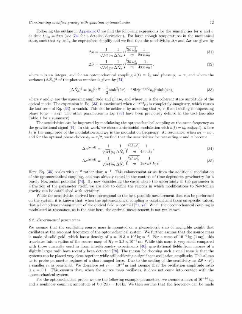
6.2. Experimental parameters

We assume that the oscillating source mass is mounted on a piezoelectric slab of negligible weight thatoscillates at the resonant frequency of the optomechanical system. We further assume that the source massis made of solid gold, which has a density of ρ = 19.3 × 103 kg m−3. For a mass of 10−6 kg (1 mg), thistranslates into a radius of the source mass of RS = 2.3 × 10−4 m. While this mass is very small comparedwith those currently used in atom interferometry experiments [40], gravitational fields from masses of aslightly larger radii have recently been detected [78]. The reason for choosing such a small mass is that thesystems can be placed very close together while still achieving a significant oscillation amplitude. This allowsus to probe parameter regimes of a short-ranged force. Due to the scaling of the sensitivity as ∆θ ∼ r2

0,a smaller r0 is beneficial. We therefore set r0 = 10−3 m and assume that the oscillation amplitude ratiois ε = 0.1. This ensures that, when the source mass oscillates, it does not come into contact with theoptomechanical system.

For the optomechanical probe, we use the following example parameters: we assume a mass of 10−14 kg,and a nonlinear coupling amplitude of k0/(2π) = 10 Hz. We then assume that the frequency can be made


as low as ωm/(2π) = 100 Hz, which is important since the expressions for ∆κ and ∆σ scale with ω5/2m . For

the squeezed coherent state, we assume that the coherent state parameter is given by |µc|2 = 106 and thatthe phase of the squeezed light can be set to ϕ = π, which ensures that the photon number variance (∆Na)2

shown in Eq. (33) is maximized. One of the highest squeezing factors that have been achieved to-date isr = 1.73 [99]. We also assume thatM = 103 measurements are performed on the system at time t ωm = 20πafter the system has been initialised.

To derive the bounds on the chameleon parameters M and Λ, we assume that the optomechanicalsystem can be operated in high vacuum. This also helps in terms of mitigating mechanical noise; in genericoscillators, damping effects are well-understood and largely not present below 10−7 mbar [100]. On the otherhand, it can be challenging to confine a levitated optomechanical system at high vacuum [101]. Recently,however, several works have demonstrated trapping at 10−7 mbar of pressure [101, 102], even going as lowas 9, 2× 10−9 mbar [103]. Using these values as our starting point, we note that 10−9 mbar translates into amolecular background density of ρbg = 8.27×10−14 kg m−3. Here, we have used the ideal gas law, which canbe rewritten to give ρbg = PmN2/(kBT ), where P is the pressure (in Pascal), kB is Boltzmann’s constant, Tis the temperature (in Kelvin), and where we have assumed that the vacuum chamber has been vented withhydrogen of molecular mass mH = 3.3× 10−27 kg.

With these parameters, we can now compute the sensitivities shown in Eqs. (31), (32), (34), and (35).We find that for a constant optomechanical coupling, the sensitivities become ∆κ = 1.36 × 10−3 and∆σ = 27.1 × 10−3. For a time-dependent optomechanical coupling modulated sinusoidally at resonance,we find the slightly better sensitivities ∆κ(mod) = 2.71× 10−3 and ∆σ(mod) = 1.73× 10−3.

Table 1. Example parameters used to compute the bounds on modified gravity for a generic optomechanicalsensor. We denote the optomechanical (probe) mass by m so as to not confuse it with the Planck mass MP.

Parameter Symbol Value

Source mass MS 10−6 kg

Source mass density ρS 19.3× 103 kg m−3

Source mass radius RS 2× 10−4 m

Equilibrium distance r0 10−3 mSource oscillation amplitude ε 0.1

Background density ρbg 8.27× 10−14 kg m−3

Optomechanical coupling k0/(2π) 10 HzMechanical frequency ωm/(2π) 100 Hz

Probe mass m 10−14 kg

Oscillator (probe) mass density (silica) ρP 1 538 kg m−3

Coherent state parameter |µc|2 106

Squeezing parameter r 1.73

Number of measurements M 103

Time of measurement ωm t = 2πn n = 10Sensitivities (constant coupling)

Sensitivity κ ∆κ 1.36× 10−3

Sensitivity σ ∆σ 27.1× 10−3

Sensitivities (resonant coupling)

Sensitivity κ ∆κ(mod) 2.71× 10−3

Sensitivity σ ∆σ(mod) 1.73× 10−3

6.3. Bounds for the Yukawa parameters α and λ

We are now ready to compute the bounds on the parameter ranges that could potentially be tested with aquantum optomechanical system. To find the bounds, we consider the ratios ∆κ/κ and ∆σ/σ as functionsof α and λ, where κ and σ were defined in Eq. (24) as the modification due to the gravitational force at


10 5 10 4 10 3 10 2 10 1 100

(m)10 8

10 6

10 4

10 2

100

102

104

106

108

||

/(mod)/(mod)//

(a)

10 15 10 13 10 11 10 9 10 7 10 5 10 3 10 1 101

M/MP

10 12

10 10

10 8

10 6

10 4

10 2

100

102

(eV)

SS = 0SP = 0

(mod)//(mod)(scr) /(scr)/

(b)

Figure 2. Ideal bounds for detecting modifications to Newtonian gravity with an optomechanical sensor.Each bound shows where the value of the modification is greater than the error bound. The parameters usedin both plots are shown in Table 1. Plot (a) shows the bounds for the Yukawa parameters α and λ. Thedashed dark green line indicates where ∆κ/κ = 1, and the dotted lighter green line where ∆κ(res)/κ = 1.The light purple area shows the parameter regime where ∆σ(res)/σ < 1 and the dark purple area shows where∆σ/σ < 1. Since κ is a constant effect, modulating the optomechanical coupling yields no improvement ofthe sensitivity. Plot (b) shows the bounds for the chameleon parameters M in terms of the Planck massMP and Λ in eV. The bounds include a point-particle approximation of the sensor (the two largest lighterpurple areas) and the inclusion of screening from a spherical probe (darker purple lines). The magentadotted lined shows where the screening length of the source mass is zero SS = 0, below which the screeningof the probe starts reducing the sensitivity. Similarly, the orange dashed line shows where the screeninglength of the probe is zero SP = 0, below which the screening of the spherical probe reduces the sensitivity.We have refrained from plotting the bounds ∆κ/κ and ∆κ(mod)/κ here as they roughly follow the outlineof the bounds on σ.

the equilibrium distance and the amplitude of the time-dependent contribution. The result can be found inFig. 2a: the dark green dashed line shows where the relative error satisfies ∆κ/κ = 1, and the dotted greenline shows where ∆κ(mod)/κ = 1. Since κ corresponds to the static modification of the gravitational force,modulating the optomechanical coupling does not improve the sensitivity. We instead focus on the dynamiccontribution from σ. The lighter purple region shows where ∆σ/σ < 1, and the darker purple region showswhere ∆σ(mod) < 1. The resonantly modulated optomechanical coupling provides a significant enhancementfor ∆σ.

The general features in Fig. 2a can be understood by examining the form of κ and σ, which are shownin Eq. (24). When λ r0, the exponential can be approximated as e−r0/λ ∼ 1. This means that σ becomesσ ∼ 2α, which is independent λ and thereby explains the straight line at |α| ∼ 10−3. Once λ < r0, whichcorresponds to a short-ranged Yukawa force, the effect can no longer be seen by the optomechanical probe.However, the bounds in Fig. 2a could be shifted to the left by decreasing r0. Care must be taken that thetwo systems do not touch, which is limited by the source sphere and probe radii, as well as the oscillationamplitude ε. For the example parameters used here, the smallest distance between the system is 0.7 mm.

6.4. Bounds for the chameleon parameters M and Λ

To obtain the bounds on M and Λ, we rescale M in terms of the reduced Planck mass MP. We then computethe bounds for M and Λ by plotting ∆σ/σ as a function of M and Λ for the following two cases: (i) whenthe probe is approximated as a point-particle (no probe screening), and (ii) when the screening from the

probe is taken into account. The latter we denote by ∆σ(scr) and ∆σ(mod)(scr) . We compute these quantities by


10 5 10 4 10 3 10 2 10 1 100

(m)

10 8

10 6

10 4

10 2

100

102

104

106

108

||

This work

(a)

10 15 10 13 10 11 10 9 10 7 10 5 10 3 10 1 101

M/MP

10 12

10 10

10 8

10 6

10 4

10 2

100

102

(eV

)

This workThis work (screened)

(b)

Figure 3. Comparison between predictions (this work) and known experimental bounds (pink region). Bothplots show the convex hull (yellow) of the bounds derived in this work in Fig. 2. Plot (a) shows the boundsin terms of the Yukawa parameters α and λ, while Plot (b) shows the bounds in terms of the chameleonscreening parameters M and Λ. Plot (b) also includes the bounds (yellow) for when the optomechanicalprobe contributes to the screening of the chameleon field. The pink areas represent the experimentallyexcluded regions based on Fig. 8 of [104] and recent results presented in [105] (see Fig. 6). (b) shows boundsin terms of M and Λ, which are the mass and energy-scale for the chameleon screening mechanism. Theexperimentally excluded regions are based on those reported in Ref [106].

numerically solving Eq. (13) for SS and SP at each point. The expression for σ given in Eq. (28).The result can be found in Fig. 2b. Note that we do not plot the bounds for ∆κ and ∆κ(mod) for clarity,

and because as static contributions they are more difficult to distinguish from a constant noise floor. Thelighter regions show the bounds when the optomechanical probe does not contribute to the screening of thefifth force. This is equivalent to approximating the probe as a point-particle. In contrast, the darker regionsshow the reduction in sensitivity due to the screening that arises from a spherical optomechanical probe.

To explain the features of the plot, we draw lines where the screening from the probe SP and sourcesystem SS vanishes. The magenta line shows where SS = 0 and the orange line shows where SP = 0. Aboveeach line, the screening is zero, while below the lines, the screening lengths increase and the modificationsto Newtonian gravity can no longer be detected. Finally, the right-most boundary of the dark purple areacan be understood as follows: The appearance of M−3 in mbg (see Eq. (11)) ensures that, when M is largecompared with the other quantities, mbg is small. This, in turn, means that the range of the force λbg, asshown in Eq. (15) will be large. It then follows that the amplitude σ (see Eq. (28)) will be approximatelyσ ≈ αbg,P , where αbg,P = 2M2/M2

P from Eq. (19) (note that ξS = ξP = 1 because we are considering therange of Λ above the orange and magenta lines). This means that σ is independent of Λ and the boundarybecomes a vertical line. The point at which the ratio ∆σ/σ = 1 then occurs is M/MP = 48.1.

7. Discussion

In this section, we compare our results with previously established experimental bounds. We also discusschallenges we expect to encounter, such as forces that arise from the Casimir effect.

7.1. Relation to existing experimental bounds

To see how the bounds in Fig. 2 relate to known experimental bounds on Newtonian gravity, we plot theconvex hull of the shaded areas in Figs. 2a and 2b against the bounds presented in Refs. [104–106]. The


results can be found in Fig. 3, where Fig. 3a shows the bounds in terms of α and λ, and where Fig. 3b showsthe bounds in therms of M and Λ. The yellow regions show the convex hull of the bounds derived in thiswork, and the pink region shows the combined parameter spaces that have been experimentally excluded.The orange area in Fig. 3b shows the excluded region for when the optomechanical probe is approximatedas a point-particle.

Our results indicate that, for the values used in this work, even the ideal realisation of a nonlinearoptomechanical sensor achieves similar bounds on α and λ to those already reported in the literature. Thedecoherence, dissipation and thermalisation effects not accounted for in this description are likely to furtherreduce the sensitivity. This suggests that the sensitivity of the system must be improved further, should wewish to probe the hitherto unexplored regions in Fig. 3a. From inspecting Eqs. (31), (32), (34), and (35),we note that the strongest dependence is with the mechanical frequency ωm. Thus the lower ωm is, thebetter the sensitivity. Another strategy would be to increase the strength of the light–matter coupling k0,however this is a long-standing challenge for many experimental platforms. More effective perhaps wouldbe to decrease the separation distance r0 between the probe and source systems, which would allow theoptomechanical sensor to explore a larger range of λ, in particular smaller λ, since the Yukawa potentialwill not be as suppressed there. However, as the sensor is moved closer to the source sphere, the Casimireffect is expected to strongly contribute to the resulting acceleration (see below). On the other hand, ourresults according to Fig. 3b indicate that optomechanical systems could be used to probe some hithertounexplored regions of the chameleon parameters M and Λ. The advances here likely depend on the qualityof the background vacuum.

7.2. Experimentally detecting modified gravity

In order to definitely rule out modifications to the Newtonian potential, an experiment must compare theobserved data with the predicted dynamics induced by the Newtonian contribution to the gravitationalpotential. This would require knowledge of the full dynamics of the system down to the desired precisionof the experiment. With this in mind, we examine the derivation of the linearized gravitational potential(see the expansion in Eq. (3)). We assumed that the perturbation δx to the position of the optomechanicalelement is small compared with xS(t) (the distance from the probe to the source mass) at all times. However,depending on the intended precision of the measurement of the force, Newtonian gravitational terms of second

order in δx may become relevant, that is terms of the form ∝(b† + b

)2. Moreover, the radiation pressure

found in an optomechanical setup has the explicit effect of displacing the mechanical element. In fact, whenthe light-matter coupling is modulated at mechanical resonance, the maximum position increases linearlyas a function of time [74]. A method for dealing with a displacement driven by radiation pressure wouldbe attempting to cancel the expected radiation pressure by manually introducing a time-dependent linearpotential into the dynamics [74]. The drawback of this method is that it most likely introduces more noiseinto the experimental setup. Another option to deal with terms of second or higher order in the mechanicalposition is to include them into the full dynamical analysis, which has been done in [107]. However, weexpect a metrology analysis to only lead to small adjustments of the bounds presented here, and thereforeleave this analysis to future work.

7.3. Limitations due to the Casimir effect

Due to the relative weakness of gravity compared with electromagnetic force, the latter are likely to dominateany experimental setting. Therefore, any stray electromagnetic effects must be controlled very precisely inorder to detect deviations from Newtonian gravity. One of the most important effects that has to be takeninto account is the Casimir force [108], which becomes significant when the distance between the probe andthe source mass is small. To estimate the effect of the Casimir force, we use an analytic formula given in [109](based on the results of [110]) for the force due to the Casimir effect between two homogeneous perfectlyconducting spheres at a distance much larger than their radii. The model of two perfectly conductingspheres is unlikely to accurately describe the experimental realisation of optomechanical setup described inthis article, both in terms of geometry and material. Therefore, we will use this case to give only a firstestimate of the effect and discuss how to suppress it.

We consider the Drude boundary condition model for isolated conductors (see [109] for details). For


the distance between the probe and the source r0 being much larger than the thermal wavelength, i.e.r0 λT = ~c/(2πkBT ) (where the thermal wavelength is about 1µm at room temperature) the classicalthermal contribution to the Casimir force dominates, which leads to the expressions

FC = 6kBTR3SR

3

r70

, (36)

where R and RS are the radii of the probe and the source, respectively. At room temperature and for theparameters given in Table 1, Eq. (36) leads to an acceleration of the order of 4 × 10−15 m s−2, experiencedby the probe mass, while the gravitational acceleration induced by the source mass is of the order of6 × 10−11 m s−2. This shows that the Casimir effect is a relevant systematic that has to be controlled.One way to do so is to lower the temperature of the setup.

Another option to suppress the Casimir effect is to place a material in-between the source mass andthe sensor that acts as a shield to the Casimir effect [111, 112]. The Casimir force of the shield will bestationary while the un-shielded gravitational acceleration will be time-dependent, and therefore, clearlydistinguishable [113]. This approach is, however, limited by the size of the shield. For example, in levitatedoptomechanics, the screening scheme can be naturally realized by placing the source mass behind one of thecavity end mirrors such that the mirror serves as a shield. However, in the case of detecting modificationsdue to a chameleon field, the presence of the mirror might introduce additional screening effects that need tobe accounted for. The Casimir effect may also be reduced by modulating or compensating for the Casimirforce with radiation pressure [114], nano-structuring of the source and probe surfaces [115], or an opticalmodulation of the charge density [116].

8. Conclusions

In this work, we derived the best-possible bounds for detecting modified gravity with a quantumoptomechanical sensor. We modelled the effects of a force from an oscillating source mass on theoptomechanical probe and estimated the sensitivity of the system by computing the quantum Fisherinformation. In particular, we considered the additional screening that arises due to the relatively largesize of the optomechanical probe. Our results show that optomechanical sensors could, in principle, be usedto improve on existing experimental bounds for the chameleon screening mechanism. While a realisticexperimental setup will likely be affected by optical and mechanical decoherence, as well as detectioninefficiencies and other systematics, our results can be used to evaluate the inherent ability of a systemto probe a particular regime.

There are a number of ways in which the sensitivity of the optomechanical system can be furtherimproved. In this work, we considered spherical source masses and probes in order to analytically derive thescreening from the probe, however, choosing a different shaped source may improve the bounds that couldbe achieved. For example, a source mass in the form of a slab much larger than the probe system wouldmitigate gradient contributions from the Newtonian part of the potential, since the gravitational force froman infinite plane is constant. Furthermore, it was shown in Ref [90] that symmetric source masses tend to bemuch more strongly screened (and thus have smaller detectable effects) then asymmetric sources. Therefore,we would expect to obtain more favourable precision bounds than those presented in this work by consideringasymmetric sources. An interesting prospect also arises from the fact that the optomechanical probe itselfcan also be asymmetric, e.g. in the shape of a levitated rod [117], which offers an additional avenue comparedwith, for example, atomic systems. However, these non-spherical cases bring with them additional challenges.The approximation used in Eq. (12) assumes a spherical source (probe), and approximates the nonlinearsolution of the chameleon field equation with an analytic expression derived by asymptotic matching. Toaccurately obtain measurements with a non-spherical setup would require precise numerical modelling of thechameleon field around a (non-spherical) source and probe, such as done in Ref [90]. The precise effect onthe sensitivity is left to further work.

In order to predict the sensitivity that an actual experiment with a optomechanical system in thenonlinear regime can achieve, we must first address several challenges. These include a quantum metrologyframework for mixed states, as well as descriptions of measurement outcomes and the inclusion of an opticaldrive. A preliminary step towards modeling Markovian optical decoherence on the intra-cavity state was


recently taken [118], but more work is needed in order to derive the resulting sensitivity and the measurementthat optimises it.

Data availability statement

The code used to compute the screening and sensitivity to chameleon fields can be found in the followingonline GitHub repository: https://github.com/sqvarfort/modified-gravity-optomech.

Acknowledgments

We thank Markus Rademacher, Niall Moroney, David Edward Bruschi, Doug Plato, Alessio Serafini, DanielBraun, Michael R. Vanner, Peter F. Barker, Clare Burrage, and Hendrik Ulbricht for helpful comments anddiscussions. S.Q. is supported by an Engineering and Physical Sciences Research Council (EPSRC) DoctoralPrize Fellowship, and D.R. would like to thank the Humboldt Foundation for supporting his work withtheir Feodor Lynen Research Fellowship and acknowledge funding by the Marie Sk lodowska-Curie Action IFprogram – Project-Name ”Phononic Quantum Sensors for Gravity” (PhoQuS-G) – Grant-Number 832250.S.S. is supported by the Royal Society, and partially supported by the UCL Cosmoparticle Initiative andthe European Research Council (ERC) under the European Community’s Seventh Framework Programme(FP7/2007-2013)/ERC grant agreement number 306478-CosmicDawn.

Appendix A. The Chameleon mechanism

In this appendix we briefly review the derivation of the chameleon mechanism and how it gives rise to afifth-force; the reader is directed to Refs [12–14] for further details. Throughout this appendix we will useenergy units (~ = c = 1) for notational simplicity. The basic idea of the chameleon screening mechanism is toscreen the effects of additional degrees of freedom in a modified gravity model (typically light scalar fields),by making their mass dependent on the local density. This results in a scalar field whose mass is large insidethe solar system where the average density is high and is thus difficult to create in collider experiments,but has a lighter mass in the intergalactic medium where the density of matter is lower. Typically, this isachieved using a scalar field whose action is of the form:

S =Sm(ψ(m),Ω−2(φ)gµν)

+

∫d4x√−g[

1

16πGR− 1

2∇µφ∇µφ− V (φ)

], (A.1)

where gµν is the spacetime curvature, R is the Ricci tensor, V (φ) is the chameleon potential, and S(m) isthe matter action. Various choices of screening mechanism are possible with this action, but the Chameleonmechanism corresponds the following choice of the functions V (φ) (the interaction potential) and Ω(φ) (whichrepresents direct, non-minimal coupling between the Chameleon field and gravity):

V (φ) =Λ4+n

φn, (A.2)

Ω(φ) = 1− φ

M. (A.3)

In this work, we will consider the case n = 1 for simplicity. One way to understand the effect of the Ω(φ) termis to regard matter as coupling to the so called Jordan frame metric, gµν = Ω−2(φ)gµν , while the Chameleonfield sees a different metric, gµν , which suggests quanta of the scalar field, if we were somehow able to isolatethem, would be observed to fall differently to normal matter (violating the equivalence principle). One caneither regard gµν as the “real” metric, in which case φ has an unusual direct coupling to gravity, or gµν , inwhich case all particles have a special coupling to φ via the function Ω(φ) appearing wherever the metricdoes in the matter action, Sm. Ultimately what matters, however, is how objects will be observed to movein the presence of this scalar field. Formally, we can obtain this from the geodesic equation, since normalmatter sees the metric gµν :

d2xρ

dλ2+ Γρµν

dxµ

dλ

dxν

dλ= 0. (A.4)

https://github.com/sqvarfort/modified-gravity-optomech


If we regard gµν as the true metric, then the effect of the chameleon field is to add what appears to

be a fifth force, since when we take the Newtonian limit we can re-write Γρµν in Eq.(A.4) in terms of theNewtonian potential, ΦN and Ω to obtain:

d2xk

dλ2= −∂kΦ + ∂k log Ω(φ(x)) = −∂k(ΦN + ΦC), (A.5)

where ΦC = − log Ω(φ(x)) is an effective fifth-force potential. The strength of this fifth force is characterisedby Ω, but to compute its effects we need to know how the scalar field couples to matter. Varying Eq. (A.1)with respect to φ we obtain:

∇µ∇µφ− V ′(φ)− d log Ω(φ)

dφgµνTµν = 0, (A.6)

where Tµν is the Hilbert Stress energy tensor. For non-relativistic matter, the scalar field is sourced by thelocal matter density, with gµνTµν = −ρ, giving

∇µ∇µφ− V ′(φ) +d log Ω

dφρ = 0. (A.7)

This is equivalent to the scalar field interacting via the potential:

Veff(φ) = V (φ)− log Ω(φ)ρ. (A.8)

If we use the form Eq. (A.3), then for cases where φM , we can approximate log Ω(φ) as:

log Ω(φ) ≈ − φ

M. (A.9)

Under this approximation, the effective scalar field potential becomes

Veff(φ) = V (φ) +φρ

M. (A.10)

and the Chameleon fifth force potential is:

Φcham(x) = − log Ω(φ(x)) ≈ φ(x)

M. (A.11)

For the purposes of this work, we will consider the n = 1 chameleon field. In a region with constant massdensity ρbg, this means that the Chameleon rests at the vacuum value:

φbg =

√MΛ5

ρbg, (A.12)

for which fluctuations of the field have mass:

m2bg(ρbg) = V ′′eff(φbg) = 2

√ρ3

bg

M3Λ5. (A.13)

As expected, the mass of field fluctuations increases with the background density, which means in areas ofcomparative high density such as inside the solar system‖, the mass is large and the scalar field difficult toexcite and detect.

‖ Compared to the average density inside a cosmological void.


Appendix A.1. Chameleon Field From a Spherical Source

The chameleon field in the vicinity of a spherical source of mass MS and radius RS can be computed bysolving the Klein-Gordon equation,

d2φ

dr2+

2

r

dφ

dr− V ′eff(φ) = 0. (A.14)

This is a non-linear equation, but an approximate solution was found by Burrage et al. [33] in the limitmbgRS 0. This is valid for the atoms considered there, but in our case we may need to consider largersources. We therefore repeat the derivation of Burrage et al. [33] for the case of arbitrary mbgRS . Thefundamental strategy uses the method of asymptotic matching [119] to derive an approximate solution overfor the full domain of the differential equation, by smoothly matching together solutions valid in differentdomains.

In the strongly perturbing case (ρSR2S > 3Mφbg/(~c)), the solution reaches its equilibrium value, φS ,

for density ρS at some radius S ≤ RS . We denote the region with r < S the interior region, or region I. Thesolution there can thus be approximated as constant

φI(r) = φS . (A.15)

There is then a transition layer (region II) between S < r < RS where the solution rapidly shifts towardsthe background value, φbg. Since the density ratio between the source-sphere and the external vacuum ishigh, we will find φbg φS as a result of Eq. (A.12). In the transition layer (S < r < RS), the field willbegin to increase, eventually reaching a regime where φ φS . Because we can re-write Eq. (A.10) as

Veff(φ) =ρφ

M

[φ2S

φ2+ 1

], (A.16)

then once φ φS the density-dependent term dominates the potential. Under such conditions, V ′eff(φ) ≈ρ/M and we can solve Eq. (A.14) analytically:

φII(r) =MS

8πMRS

r2

R2S

+C

r+D. (A.17)

Finally, far away from the source sphere, φ is close to its background value, φbg, and we can approximatethe potential as quadratic: Veff(φ) ≈ m2

bg(φ− φbg)2/2. The solution there takes the form

φIII(r) = φbg +E

re−mbgr +

F

re+mbgr. (A.18)

Here, region III is defined as r > RS . Note that although φ φS outside the sphere, Eq. (A.17) doesnot apply because the density outside the sphere is now ρbg which is typically much smaller than ρS : thedensity dependent term in the potential is thus no longer dominant outside the source. We note, however, thatsolutions φII and φIII are technically only valid in the vicinity of r ∼ RS and r RS respectively. However,we can approximate the behaviour of the fully-non-linear solution for all r by matching these asymptoticsolutions at S and RS , which imposes four constraints to ensure smoothness of the asymptotically matchedsolution: φI(S) = φII(S), φ′I(S) = φ′II(S), φII(RS) = φIII(RS), φ′III(RS) = φ′III(RS). We also note thatwe require F = 0 to have a solution approaching φbg as r →∞, which means that there are four unknowns,C,D,E, and the radius S. We solve for these four unknowns, finding

C =MS

4πM

S3

R3S

, (A.19)

D =φS −3MSS

2

8πMR3S

, (A.20)

E =− MS

4πM(1 +mbgRS)

(1− S3

R3S

)embgRS , (A.21)


where S satisfies

S2S

R2S

+2

3

[1

1 +mbgRS− 1

]S3S

R3S

= 1− 8πM

3MSRS(φbg − φS) +

2

3

[1

1 +mbgRS− 1

]. (A.22)

Taken together, Eqs (A.19)–(A.21) and (A.22) imply Eq. (12), and reduce to the Burrage et al. [33] resultin the case mbgRS → 0 limit. As a cubic equation for S, it is of limited use to express S in closed form, andfor the purposes of this work we solve Eq. (A.22) numerically. This can run into catastrophic cancellationproblems, due to the finite floating-point precision, when S ≈ RS (that is, the heavily screened regime),since we need to compute 1− S3/R3

S . Hence, when the numerical solution gives S/RS close to 1, we switchover to an analytic approximation obtained by substituting S/RS = 1 + ε and solving for ε to first order.This gives

ε = −4πM

3MSRS(φbg − φS)(1 +mbgRS), (A.23)

which implies

1− S3

R3S

≈ 4πM

MSRS(φbg − φS)(1 +mbgRS). (A.24)

We see that Eq. (A.24) agrees with the Taylor expansion of Eq. (14) in the mbgRS → 0 limit.

Appendix B. Time dependence of a chameleon field

The main result of this work is that an oscillating optomechnanical system can be used to detect the presenceof chameleon fields. However, throughout we have made the assumption that such a field responds essentiallyinstantaneously to the motion of the mass that sources it. For purely gravitational effects this assumption isjustified since information about the position of the source mass propagates outwards at the speed of light.However, the situation is less clear for a scalar field sourced by a moving mass, since the field is massive:there is no a priori guarantee that information can propagate outwards at the speed of light. To address this,we derive the propagator for a chameleon field sourced by a point mass and demonstrate that the resultingretarded chameleon potential can be treated as if information propagates instantaneously, for non-relativisticoscillating masses.

Appendix B.1. Time dependence of the gravitational potential

First, we will derive the response of the gravitational field to a small mass, neglecting back-reaction andgravitational wave emission as negligible. In the linearised limit which allows us to make contact withNewtonian gravity, the metric perturbation hµν around ηµν satisfies:

∂σ∂νhσµ + ∂σ∂µh

σν − ∂µ∂νh− ∂λ∂λhµν

−ηµν∂ρ∂λhρλ + ηµν∂λ∂λh = 16πGTµν , (B.1)

where we are using the − + ++ metric convention. We choose the Lorenz gauge, defined by the condition∂µh

µν = 12∂

νh, which simplifies this to:

∂λ∂λhµν = −16πGTµν , (B.2)

where hµν = hµν − 12hηµν is the trace-reversed perturbation. A generic expression for the Hilbert stress

energy tensor is:

Tµν = − 2√−det g

δSmδgµν

, (B.3)

where Sm is the matter action. For a point particle of mass MS , the appropriate matter action is:

Sm = MS

∫dτ√−gµν qµqν , (B.4)


where qµ(τ) describes the particle trajectory and dots denote differentiation with respect to proper time,τ (the variation with respect to qµ yields the geodesic equation, verifying that this is indeed the action weseek). This means that the stress-energy tensor for a point particle is:

Tµν =MS qµqνδ

(3)(x− q(τ))√−det g

√−gαβ qαqβ

. (B.5)

For low (non-relativistic) velocities in a Minkowski background this means T00 = MSδ(3)(x− q(τ)) = ρ, as

we would expect, with all other components zero. Note that we are ignoring any back-reaction from thismoving particle, which would give only higher order corrections. Taking the trace of Eq. (B.2) yields:

∂λ∂λh = −16πGρ, (B.6)

which is the same equation satisfied by h00, and so we have h = h00 (note the sign – ηµν hµν = −h, butηµνTµν = −ρ). Meanwhile, ∂λ∂

λhij = 0 as there are no spatial parts of Tµν . This describes propagatinggravitational waves, which we neglect, and can be safely set to zero. Thus, we need only solve Eq. (B.6),which has a known solution in terms of a retarded potential:

h = 4G

∫d3x′

ρ(t− |x−x′|

c ,x′)

|x− x′|. (B.7)

For the point source with density ρ(x, t) = MSδ(3)(x− q(t)), this means:

h(x, t) =4GMS

|x− q(tret)|. (B.8)

where tret is the retarded time that solves:

tret = t− |x− q(tret)|c

. (B.9)

Note, comparing with the standard perturbative parameterisation of the metric:

ds2 =− dt2(1 + 2Φ) + wi(dxidt+ dtdxi)

+ [(1− 2Ψ)δij + 2sij ]dxidxj , (B.10)

we see that Φ = −h/4, or in other words:

Φ(x, t) = − GMS

|x− q(tret)|, (B.11)

which is the retarded gravitational potential for a point source of mass M , as we would expect. Note that thisis well defined (in the Lorenz gauge), as it is not derived from energy considerations but from the equationof motion of the metric perturbation.

Appendix B.2. Time dependence of the chameleon field

The evolution of the scalar field is significantly more complicated, due to the fact that it satisfies a highlynon-linear equation of motion, Eq. (A.6). However, provided the source mass is not large the we can considersmall deviations from the background value φbg and linearise the equation:

∂λ∂λ∆φ−

m2bgc

2

~2∆φ =

∆ρ(x, t)

M, (B.12)

where ∆φ = φ − φbg and ∆ρ is the deviation from ρbg that sources the field deviation. This is the Klein–Gordon equation with mass mbg, but with a source on the RHS. To solve this, we need to make use of the


retarded propagator of the Klein–Gordon equation [120]:

Gret(x, y) =Θ(x0 − y0)

2πδ(τ2(x, y)) (B.13)

−Θ(x0 − y0)Θ(τ2(x, y))mbgcJ1(mbgcτ(x, y)/~)

4π~τ(x, y),

τ(x, y) =√c2(x0 − y0)2 − (x-y)2. (B.14)

Here, J1 is a Bessel function of the first kind. Note that we choose the retarded, rather than advanced orFeynman propagator here in order to ensure that the field responds causally to the movements of the source.The general solution of Eq. (B.12) is

∆φ(x) =

∫d4x′

∆ρ(x′)

MGret(x, x

′). (B.15)

For our point particle, the density deviation is

∆ρ(x, t) = MSδ(3)(x− q(t)). (B.16)

The corresponding solution is thus:

φ(x, t) = φbg +MSc

M

∫dt′[θ(t− t′)

2πδ(c2[t− t′]2 − |x− q(t′)|2)

− θ(t− t′)θ(c2[t− t′]2 − [x− q(t′)]2)mbgcJ1(mbgc

√c2(t− t′)2 − |x− q(t′)|2/~)

4π~√c2(t− t′)2 − |x− q(t′)|2

]. (B.17)

We use the formula:

δ(f(x)) =∑i

δ(x− xi)|f ′(xi)|

, (B.18)

where xi are solutions of f(xi) = 0. In the q constant case, it is easy to see that there are two solutions,t′ = t±|q−x|, but only the negative solution matters, due to the θ(t−t′) term (this is the causal effect of theretarded propagator, and ensures that we only integrate over contributions from the past of the time t we arelooking at). In the case where q is time dependent, solving (t− t′)2 − |x− q(t′)|2 = 0 is less trivial, but stillresults in a unique retarded time, tret, exactly the same quantity that is well known from electrodynamics.To see that it is unique, consider that tret is by definition the time at which light arriving at an observer attime t was emitted by the source. Assume there are two such times, t1, t2. We have (temporarily puttingback the factors of c for clarity) c(t− ti) = |q(ti)−x|, and can subtract these two equations from each otherto obtain c(t2− t1) = |q(t1)−x| − |q(t2)−x|. This implies that the distance of q from x has changed at thespeed of light - not possible unless the source itself is moving at the speed of light. Thus, for sub-luminalsources, tret is unique¶. Hence:

δ(c2[t− t′]2 − |x− q(t′)|2) =δ(t′ − tret)

2(c2(tret − t) + (x− q(tret)) · v(tret))

= − δ(t′ − tret)

2c|x− q(tret)|(1− (x−q(tret))|x−q(tret)| · v(tret)/c)

, (B.19)

where we have used Eq. (B.9) and v(t) is the velocity of the source. Thus, the first part of the integralreduces to:

I1 = − MS

4πM |x− q(tret)|(1− (x−q(tret))·v(tret)|x−q(tret)|c )

. (B.20)

¶ Actually, there is still a solution for tadv > t, but this is eliminated due to the causal θ(t− t′) function.


This is indeed exactly the same as the expression found in electrodynamics, where the propagating field (thephoton) is massless, and thus the second term in Eq. (B.17) is not present. In our case, however, we have todeal with the massive part of the integral too:

I2 =− cMS

4πM

∫dt′θ(t− t′)θ(c2[t− t′]2 − |x− q(t′)|2)

(mbgcJ1(mbgc

√c2(t− t′)2 − |x− q(t′)|2/~)

~√c2(t− t′)2 − |x− q(t′)|2

).

In this case, the effect of the two Heaviside step functions is to force us to integrate over the past, up to theretarded time:

I2 = − cMS

4πM

∫ tret

−∞dt′

mbgcJ1(mbgc√c2(t− t′)2 − |x− q(t′)|2/~)

~√c2(t− t′)2 − |x− q(t′)|2

. (B.21)

Now, make the substitution:

u =mbgc

~√c2(t− t′)2 − |x− q(t′)|2, (B.22)

t′(u) =t− ~c2mbg

√u2 +

m2bgc

2

~2|x− q(t′(u))|2, (B.23)

du =mbgc[c

2(t′ − t) + (x− q(t′)) · v(t′)]

~√c2(t− t′)2 − |x− q(t′)|2

dt′, (B.24)

to obtain:

I2 = +mbgcMS

4πM~

∫ ∞0

duJ1(u)√

u2 +m2bgc

2|x− q(t′(u))|2/~2 − [x− q(t′(u))] · v(t′(u))mbg/~. (B.25)

This would not seem to offer a significant simplification, unless we adopt the low-velocity approximation,|v0|/c 1. The second term in the denominator is O(v/c), so we can in general neglect it (note that|x − q(t′)|/c is not in general small as x can be arbitrarily far from the source). We can also expand|x− q(t′(u))|2 as a power series in u around the retarded time, tret = t′(0):

|x− q(t′(u))|2 = |x− q(tret)|2 +d|x− q(t′)|2

dt′

∣∣∣∣t=tret

dt′

duu+

d2t′

du2

d|x− q(t′)|2

dt′

∣∣∣∣t′=tret

u2

2

+

(dt′

du

)2d2|x− q(t′)|2

dt′2


u2

2+O(u3). (B.26)

We find:

d|x− q(t′)|2

dt′= −2(x− q(t′)) · v(t′),

d2|x− q(t′)|2

dt′2= 2|v(t′)|2 − 2(x− q(t′)) · dv′

dt′, (B.27)

dt′

du=

~√c2(t− t′)2 − |x− q(t′)|2

mbgc[c2(t′ − t) + (x− q(t′)) · v(t′)], (B.28)

d2t′

du2=

~mbgc

√c2(t− t′)2 − |x− q(t′)|2

(dt′

du

)−

~√c2(t− t′)2 − |x− q(t′)|2

mbgc [c2(t′ − t) + (x− q(t′)) · v(t′)]2 ×

[c2 − |v(t′)|2 + (x− q(t′)) · dv(t′)

dt′

]dt′

du. (B.29)


And evaluated at u = 0 (or t′ = tret), this gives:

d|x− q(t′)|2

dt′


= −2(x− q(tret)) · v(tret), (B.30)

d2|x− q(t′)|2

dt′2


= +2|v(tret)|2 − 2(x− q(tret)) ·dv′

dt′


, (B.31)

dt′

du

∣∣∣∣u=0

= 0, (B.32)

d2t′

du2

∣∣∣∣u=0

=~2

m2bgc

2 [c2(tret − t) + (x− q(tret) · v0(tret))]. (B.33)

Hence:

|x− q(t′(u))|2 = |x− q(tret)|2 −~2(x− q(tret)) · v(tret)

m2bgc

2 [c2(tret − t) + (x− q(tret) · v(tret))]u2 +O(u3).

We substitute in Eq. (B.9) to obtain

|x− q(t′(u))|2 = |x− q(tret)|2 +~2 (x−q(tret))|x−q(tret)| · v(tret)/c

m2bgc

2[1− (x−q(tret))

|x−q(tret)| · v(tret)/c]u2 +O(u3).

The u2 term is proportional to v/c once SI units are restored and so we can ignore it in the non-relativisticlimit. Generally speaking, higher order terms in the expansion about u = 0 will also have terms proportionalto v/c 1, so we neglect them+. This reduces the integral to:

I2 = +MSmbgc

4πM~

∫ ∞0

duJ1(u)√

u2 +m2bgc

2|x− q(tret)|2/~2

= +MS

4πM |x− q(tret)|

(1− e−mbgc|x−q(tret)|/~

). (B.34)

Combining this with Eq. (B.20), again in the v c limit, gives:

∆φ(x, t) = − MS

4πM |x− q(tret(x, t))|e−mbg|x−q(tret(x,t))|. (B.35)

This is the expected Yukawa potential, only with the retarded time for the position of the source. It isworth noting that the fact that the force carrier (in this case the scalar bosonic chameleon field excitations)is massive does not appear to affect the retarded time, which describes information propagating throughthe field at the speed of light, even though the bosons themselves do not. The fact that the retarded timeappears, both here and in electrodynamics, is not because the force carriers themselves (photons in the caseof electrodynamics) travel at the speed of light - it is due to the causal structure of space-time itself.

Appendix B.3. Screening by the optmomechanical Probe

Burrage et al. [33] derived an expression for the force between two extended spheres due to a chameleon field.However, their approach considered the forces between individual atoms, for which the range of the forcecould largely be ignored (corresponding to the mbgr 1 limit). With the larger sensor devices we consider inthis work this is not necessarily applicable. Furthermore, since in this case we envision an oscillating source,we need to be certain that time-dependent effects do not come into play. For this reason, we re-derive theforce between two spheres without the static spheres and mbgr 1 assumption. The derivation closelyfollows that of Burrage et al. [33], with the assumption of a spherical probe to provide a simplification (more

+ One can argue that this must be true for the solution to reduce to the static Yukawa potential in the v → c limit.


accurate modelling of the optomechanical probe will in principle be necessary for performing the actualexperiment).

As in Burrage et al. [33], we denote the source sphere A and the test sphere (B) for which we arecomputing the force (as a model for the optomechanical probe). The force is determined by the rate ofchange of the momentum resulting from the energy momentum flux across the surface of ball B:

Fi = Pi = −∫∂B

τ ji njdS, (B.36)

where τ ji are the spatial components of the energy momentum tensor (including gravity), ∂B is the surfaceof ball B, nj the surface normal vector and dS the surface area element. The gravitational and mattercontributions to the energy momentum tensor follow as in Burrage et al. [33], with the main change beingto the chameleon field term:

T(φ)ji = −∇iφ∇jφ+ δji

(1

2∇µφ∇µφ+ V (φ)

). (B.37)

The chameleon field at position x and time t with x centred on ball B is given by

φ(x, t) = φbg+φA(x, t)+φB(x) = φbg−ξAMA

4πM(1 +mbgRA)

e−mbg(|x−xA(t)|−RA)

|x− xA(t)|− ξBMB

4πM(1 +mbgRB)

e−mbg(r−RB)

r,

(B.38)where r = |x| and where the prefactors ξA and ξB are given by

ξi =

1, ρiR

2i < 3M φbg,

1− S3i

R3i, ρiR

2i > 3Mφbg.

(B.39)

Note that that we have assumed the linear regime, where the fields from the two chameleon sources add.The gradient of the contribution φB(x) from ball B is given by

∇iφB =ξBMB

4πM

1

r2

(1 +mbgr)

(1 +mbgRB)e−mbg(r−RB)∇ir =

ξBMB

4πM

xir3

(1 +mbgr)

(1 +mbgRB)e−mbg(r−RB). (B.40)

The chameleon stress-energy tensor is therefore given by

T(φ)ji =−

(∂iφA +

ξBMB

4πM

xir3

(1 +mbgr)

(1 +mbgRB)e−mbg(r−RB)

)(∂jφA +

ξBMB

4πM

xj

r3

(1 +mbgr)


)+ δji

[1

2

(∂kφA +

ξBMB

4πM

xkr3

(1 +mbgr)


)(∂kφA +

ξBMB

4πM

xk

r3

(1 +mbgr)


)− 1

2(∂t(φA + φB))2

], (B.41)

whereas Burrage et al. [33], we ignore the contribution from the potential, V (φ). Note that Burrage et al. [33]assume the mbgr 1 limit, which we generalise here to arbitrarily large r. To do this, we will make onlythe assumption that |x|/|xA| 1 on the surface of ball B, that is, that the radius of ball B is much smallerthan the distance to ball A. The means we can expand

|x− xA| ≈ |xA|(

1− x · xA|xA|2

+O(|x|2/|xA|2)

). (B.42)

We can then expand the derivative of the field from sphere A as

∂iφA =ξAMA

4πM |xA|2(1 + |xA|mbg)

(1 +mbgRA)exp

(−mbg(|xA| −RA) +

mbgx · xA|xA|

+O(|x|2/|xA|2)

)×[

− xAi|xA|

+ xj(δij|xA|

− 3xAixAj|xA|3

+mbgxAixAj

(1 + |xA|mbg)|xA|2

)+O(|x|2/|xA|2)

], (B.43)


where we have deliberately not expanded the exponential in |x|/|xA|. This is because we cannot generallyassume that mbg|x| << 1 (though we will examine this limit later).

We are seeking to perform an integral of the form

−∫∂B

dST(φ)ji nj . (B.44)

First, use the fact that ∂tφB = 0 (we are in the frame of reference of B, so all time dependence is in themotion of ball A). The time derivative of the field is

∂tφA =ξAMA

4πM

(x− xA) · (−vA)

|x− xA|3(1 +mbg|x− xA|)

(1 +mbgRA)e−mbg(|x−xA|−RA) = −viA∂iφA, (B.45)

which can be written in terms of the spatial derivative because the time dependence only appears throughxA, which always appears together with x in the form |x − xA|. This allows us to simplify the expressionfor the stress-energy tensor:

T(φ)ji ≈

(−δki δjl +

δji δkl

2

)(∂kφA + ∂kφB)(∂lφA + ∂lφB)− δji

2vkAv

lA∂kφA∂lφA. (B.46)

We therefore find that the integral splits into three parts:

−∫∂B

dST(φ)ji nj =IAA + IAB + IBB , (B.47)

IAA =

(δ

(ki δ

l)j − δji2

[δkl − vkAvlA]

)1

RB

∫∂B

dSxj∂kφA∂lφA, (B.48)

IAB =

(δ

(ki δ

l)j − δji2δkl

)2

RB

∫∂B

dSxj∂kφA∂lφB , (B.49)

IBB =

(δ

(ki δ

l)j − δji2δkl

)1

RB

∫∂B

dSxj∂kφB∂lφB . (B.50)

We can write

∂iφB ||x|=RB=ξBMB

4πM

xiR3B

≡ QBxi, (B.51)

where we define

QB =ξBMB

4πM

1

R3B

. (B.52)

Similarly:

∂iφA =QA(−xAi + xjAij

) (1 +mbg|xA|)(1 +mbgRA)

e−mbg(|xA|−RA) exp

(mbgx · xA|xA|

), (B.53)

QA =ξAMA

4πM

1

|xA|3, (B.54)

Aij =

[δij −

3xAixAj|xA|2

+mbgxAixAj

(1 +mbg|xA|)|xA|

]. (B.55)


This means we can write the three integrals IAA, IAB , IBB as

IAA =

(δ

(ki δ

l)j − δji2

[δkl − vkAvlA]

)Q2A

RB

[xAkxAlBj(2mbg)− (xAkAlm + xAlAkm)Bjm(2mbg)

+AkmAlnBjmn(2mbg)] (1 +mbg|xA|)2

(1 +mbgRA)2e−2mbg(|xA|−RA), (B.56)

IAB =

(δ

(ki δ

l)j − δji2δkl

)2QAQBRB

(−xAkBil(mbg) +AkmBjml(mbg))(1 +mbg|xA|)(1 +mbgRA)

e−mbg(|xA|−RA), (B.57)

IBB =

(δ

(ki δ

l)j − δji2δkl

)Q2B

RB

∫dSxjxkxl, (B.58)

where we have expressed everything in terms of the following integrals:

Bi(m) =

∫dSxie

mx·xA/|xA|, (B.59)

Bij(m) =

∫dSxixje

mx·xA/|xA|, (B.60)

Bijk(m) =

∫dSxixjxke

mx·xA/|xA|. (B.61)

In fact, one can immediately see that IBB = 0, because the integral of a cubic polynomial vanishes overa sphere: ∫

∂B

xixjxkdS = 0. (B.62)

This follows from symmetry since the integrand is odd when x→ −x and we integrate over the whole sphere(one can also verify this directly by evaluating it in spherical polar co-ordinates).

To evaluate the remaining integrals in Eqs. (B.59)-(B.61), we switch to polar co-ordinates. Withoutloss of generality, we can arrange our co-ordinates at any time to be such that xA is along the z axis, whichsimplifies the calculation. For Bi(m) we obtain

Bi(m) =

∫xie

mzdS. (B.63)

We define our polar co-ordinates as

x =r sin θ cosψ,

y =r sin θ sinψ,

z =r cos θ. (B.64)

We can see immediately that B1 = B2 = 0 since

B1 ∝∫ 2π

0

dψ cosψ = 0, B2 ∝∫ 2π

0

dψ sinψ = 0. (B.65)

We therefore only need to evaluate B3:

B3(m) = 2πR3B

∫ π

0

dθ sin θ cos θemRB cos θ =4πRBm2

(mRB cosh(mRB)− sinh(mRB)). (B.66)

We can summarise this as

Bi(m) = δi34πRBm2

(mRB cosh(mR)− sinh(mR)), (B.67)


which generalises, for an arbitrary axis choice, to

Bi(m) =xAi|xA|

4πRBm2

(mRB cosh(mRB)− sinh(mRB)). (B.68)

Next, we evaluate Bij(m). We can make similar arguments here to conclude that B13 = B23 = 0 (for thesame reason that B1 = B2 = 0). Furthermore:

B12 ∝∫ 2π

0

sinψ cosψ = 0. (B.69)

Hence, all the cross-terms vanish, so this tensor is diagonal. The diagonals are:

B11 =R4B

∫ 2π

0

dψ cos2 ψ

∫ π

0

sin3 θemRB cos θ =πRBm3

(4mR cosh(mRB)− 4 sinh(mRB)), (B.70)

B22 =R4B

∫ 2π

0

dψ sin2 ψ

∫ π

0

sin3 θemRB cos θ =πRBm3

(4mRB cosh(mRB)− 4 sinh(mRB)), (B.71)

B33 =2πR4B

∫ π

0

dθ cos2 θ sin θemRB cos θ =πR

m3(−8mRB cosh(mRB) + 4(2 +m2R2

B) sinh(mRB)). (B.72)

This can be summarised as

Bij(m) = δijπRBm3

(4mRB cosh(mRB)− 4 sinh(mRB))

+ δi3δj3πRBm3

(−12mRB cosh(mRB) + 4(3 +m2R2B) sinh(mRB)), (B.73)

or, for a generic axis choice:

Bij(m) = δijπRBm3

(4mRB cosh(mRB)− 4 sinh(mRB))

+xAixAj|xA|2

πRBm3

(−12mRB cosh(mRB) + 4(3 +m2R2B) sinh(mRB)). (B.74)

Finally, we can compute Bijk(m). First, note that this is a rank-3 symmetric tensor. Rank m symmetrictensors in d dimensions have (m + d − 1)!/(d − 1)!m! independent components, which for d = 3 gives(m+ 1)(m+ 2)/2. This means we have to compute 10 independent components in total. However, as beforemost are actually 0. Again, similar arguments to before imply B331 = B221 = B321 = 0. We also find that:

B111 ∝∫ 2π

0

dψ cos3 ψ = 0,

B222 ∝∫ 2π

0

dψ sin3 ψ = 0,

B112 ∝∫ 2π

0

dψ cos2 ψ sinψ = 0,

B221 ∝∫ 2π

0

dψ sin2 ψ cosψ = 0. (B.75)

There are, in fact, only three non-zero components:

B333 =2πR5B

∫ π

0

dθ cos3 θ sin θemRB cos θ =πRBm4

(4mRB(6 +m2R2B) cosh(mRB)− 12(2 +m2R2

B) sinh(mRB)).

(B.76)

B311 =R5B

∫ 2π

0

dψ cos2 ψ

∫ π

0

dθ cos θ sin3 θemRB cos θ =πRBm4

(−12mRB cosh(mRB) + 4(3 +m2R2B) sinh(mRB)).

(B.77)

B322 =R5B

∫ 2π

0

dψ sin2 ψ

∫ π

0

dθ cos θ sin3 θemRB cos θ =πRBm4

(−12mRB cosh(mRB) + 4(3 +m2R2B) sinh(mRB)).

(B.78)


To summarise this, we note that only terms with at least one of i, j, k equal to 3 are non-zero. The othertwo indices must then be a diagonal matrix. This means that we can write:

Bijk =δi3

[δjk

πRBm4

(−12mRB cosh(mRB) + 4(3 +m2R2B) sinh(mRB))

+δj3δk3πRBm4

(4mRB(9 +m2R2B) cosh(mRB)− 4(9 + 4m2R2

B) sinh(mRB))

]+ (all permutations).

(B.79)

Or, using symmetrised index notation:

Bijk =xA(i

|xA|

[δjk)

πRBm4

(−12mRB cosh(mRB) + 4(3 +m2R2B) sinh(mRB))

+xAixAj)

|x|2AπRBm4

(4mRB(9 +m2R2B) cosh(mRB)− 4(9 + 4m2R2

B) sinh(mRB))

], (B.80)

where for an arbitrary tensor, circular brackets around indices indicate the symmetrised indices:

M(i1...in) ≡1

n!

∑permutations

Mip1...ipn , (B.81)

where p1 . . . pn run over all permutations of 1 . . . n. For example:

M(ij) ≡1

2(Mij +Mji), (B.82)

M(ijk) ≡1

6(Mijk +Mikj +Mjki +Mjik +Mkij +Mkji). (B.83)

We can now proceed to substitute these into the expressions for IAA and IAB . First, we consider IAA, sincethis term is argued to be zero by Burrage et al. [33] in the mbgr 0 limit. First, we can ignore the velocitydependent terms, since we work in the non-relativistic limit where |vA| 0 (we are using units where c = 1).To gain some further understanding of the behaviour, let us consider the RB → 0 limit:

Bi(m) ≈ 4πxAi3|xA|m3

(mRB)4 +O((mRB)6), (B.84)

Bij(m) ≈δij4π

3m4(mRB)4 +O((mRB)6), (B.85)

Bijk(m) ≈xA(i

|xA|

[δjk)

4π

15m5(mRB)6 +

xAjxAk)

|xA|28π

15m5(mRB)6 +O((mRB)8)

]. (B.86)

This gives

IAA ≈

(δ

(ki δ

l)j − δji2δkl

)Q2A

RB

[πxAkxAlxAj

6|xA|m3bg

(2mbgRB)4 − πxAkAlj6m4

bg

(2mbgRB)4 +O((2mbgRB)6)

]

× (1 +mbg|xA|)2

(1 +mbgRA)2e−2mbg(|xA|−RA),

=

(δ

(ki δ

l)j − δji2δkl

)QAξAMA(1 +mbg|xA|)

4πMe−mbg|xA|

[8πmbgxAkxAlxAj

3|xA|

(RB|xA|

)3

− 8πxAkAlj6

(RB|xA|

)3]

× (1 +mbg|xA|)2

(1 +mbgRA)2e−2mbg(|xA|−RA), (B.87)

IAB ≈

(δ

(ki δ

l)j − δji2δkl

)2QAQBRB

[−4πxAk

3m4bg

δil(mbgRB)4 +O((mbgRB)6)

](1 +mbg|xA|)(1 +mbgRA)

e−mbg(|xA|−RA)

=

(δ

(ki δ

l)j − δji2δkl

)QA

ξBMB

4πM(1 +mbgRB)e−mbgRB

[−8πxAk

3δil

](1 +mbg|xA|)(1 +mbgRA)

e−mbg(|xA|−RA).

(B.88)


This suggests that IAA is subdominant in this limit, provided:

QAQB

(1 +mbg|xA|)(1 +mbgRA)

e−mbg(|xA|−RA) RB|xA|

. (B.89)

Then this means that we can essentially ignore the IAA term in the RB → 0 limit, which agrees with thecalculation of Burrage et al. [33]. Furthermore, provided we stay in the limit in Eq. (B.89), then IAA willalways be suppressed relative to IAB . Generally speaking, this may not be the case, however, in which casewe would have to include the IAA term. For now, let us compute the force without this term, as just includethe IAB contribution:

Fi =

(δ

(ki δ

l)j − δji2δkl

)2QAQBRB

(−xAkBjl(mbg) +AkmBjml(mbg))(1 +mbg|xA|)(1 +mbgRA)

e−mbg(|xA|−RA). (B.90)

Let us evaluate each piece in turn:(δ

(ki δ

l)j − δji2δkl

)xAkBjl(mbg) =

1

2(δki δ

jl + δji δkl − δji δ

kl)xAkBjl

=xAi2Bjj

=xAi2πR3

B

mbgsinh(mbgRb), (B.91)

where in the last line we simply add the non-zero diagonals, Eqs. (B.70) - (B.72). The next piece is slightlymore complicated: (

δ(ki δ

l)j − δji2δkl

)AkmBjml(mbg) =

1

2AimBmjj . (B.92)

Consider m = 1, 2, 3 in turn, and use co-ordinates where xA is along the z axis for simplicity. We findthat B1jj = B111 + B122 + B133 = 0, B2jj = B211 + B222 + B233 = 0 and the only non-zero component isB3jj = B311 +B322 +B333, which is obtained by summing Eqs. (B.77) - (B.76). Together this implies:

Bm33 = δm34πR2

B

m3bg

(mbgRB cosh(mbgRB)− sinh(mbgRB)). (B.93)

In the same co-ordinates, we find

Ai3 = δi3

(mbg|xA|

1 +mbg|xA|− 2

), (B.94)

which implies:(δ

(ki δ

l)j − δji2δkl

)AkmBjml(mbg) = δi3

(mbg|xA|

1 +mbg|xA|− 2

)2πR3

B

m2bg

(mbgRB cosh(mbgRB)− sinh(mbgRB)).

(B.95)


We conclude that

Fi =QAQB

[−xAi

4πR2B

mbgsinh(mbgRB) +

xAi|xA|

(mbg|xA|

1 +mbg|xA|− 2

)4πR2

B

m2bg

(mbgRB cosh(mbgRB)− sinh(mbgRB)

]

× (1 +mbg|xA|)(1 +mbgRA)

e−mbg(|xA|−RA)

=ξAξBMAMB

16π2M2|xA|3R3B

(1 + |xA|mbg)

(1 +mbgRA)e−mbg(|xA|−RA)×[

−xAi4πR2

B

mbgsinh(mbgRB) +

xAi|xA|

(mbg|xA|

1 +mbg|xA|− 2

)4πR2

B

m2bg


]

=− GξAξBMAMBM2P

2πM2|xA|2(1 + |xA|mbg)

(1 +mbgRA)e−mbg(|xA|−RA) xAi

|xA|×[

4π

mbgRBsinh(mbgRB)−

(mbg|xA|

1 +mbg|xA|− 2

)4π

m2bg|xA|RB


]

=− GMAMB

|xA|22ξAξB

(MP

M

)2(1 + |xA|mbg)

(1 +mbgRA)e−mbg(|xA|−RA) xAi

|xA|×[

1

mbgRBsinh(mbgRB)−

(mbg|xA|

1 +mbg|xA|− 2

)1

m2bg|xA|RB


].

(B.96)

Including the gravitational force, and moving to co-ordinates centred on ball A, we find:

F (r) = −GMAMB

r2

[1 + 2ξAξB

(MP

M

)2(1 + |xA|mbg)

(1 +mbgRA)e−mbg(|xA|−RA)f(mbgRB ,mbg|xA|)

], (B.97)

where we have a form-factor function that modifies the force, given by

f(x, y) = (1 + x)e−x[

sinh(x)

x−(

y

1 + y− 2

)1

y

(cosh(x)− sinh(x)

x

)]. (B.98)

This force has several peculiar features. Firstly, there appears to be a double-counting of the distancefrom the centre of ball B to its surface (RB) featuring in the exponential suppression with distance. Note,however, that this additional exponential arises from the screening affect of the probe itself, that is, its lackof response to the chameleon field when the probe is itself large. Secondly, we note that if we computed theforce of ball B on ball A, we would not obtain a symmetric force of opposite sign. In other words, this forceappears to violate Newton’s third law, which on the face of it suggest that momentum is not conserved.However, this is misleading, because the derivation takes into account the stress energy tensor not onlyof the ball itself (τ (m)µν) but of the chameleon field (τ (φ)µν). Momentum should still be conserved if themomentum of both the balls and the field are included in the calculation. This differs from the Newtonianforce derived by Burrage et al. [33] since in the mbgRB 1 limit the force is inverse-square, meaning thatNewton’s shell theorem applies; a sphere should exert the same inverse-square force as an equivalent pointmass. But this does not apply to Yukawa potentials, implying that the chameleon force does not obey thestrong equivalence principle (in addition to the explicit violation of the weak equivalence principle due tothe force being density-dependent). In any case, the form factor f is typically close to 1 (it is equal to 1 inthe mbgRB 1 limit), so can in most cases be neglected.

Appendix C. Derivation of the sensitivity

The dynamics that arise for a moving source-mass was solved in Refs [87]. Resonant gravimetry andenhancements from modulated optomechanical couplings were considered in [74]. We here outline the solutionand refer the reader to [74] for the full derivation.


Appendix C.1. Solution of the dynamics

The time-evolution that arises from the Hamiltonian in Eq. (5) can be written as

U(t) = e−i FNaNa e

−i FN2aN2

a e−i FB+

B+ e−i FNa B+

Na B+ e−i FB−

B− e−i FNa B−

Na B− , (C.1)

where we have transformed into a frame that is rotating with the free optical evolution a†a, and where theoperators are given by

N2a = (a†a)2,

Na = a†a, Nb = b†b,

B+ = b† + b, B− = i (b† − b),

Na B+ = Na (b† + b), Na B− = Na i (b† − b). (C.2)

By differentiating U(t) and equating the result with the Hamiltonian in Eq. (5), we can use the linearindependence of the Hilbert space to find the following coefficients [87]

FNa= 2

x0

~

∫ t

0

dt′ V ′(xS(t′)) sin(ωmt′)

∫ t′

0

dt′′ g(t′′) cos(ωmt′′)

+ 2x0

~

∫ t

0

dt′ g(t′) sin(ωmt′)

∫ t′

0

dt′′ V ′(xS(t′′)) cos(ωmt′′) ,

FN2a

= −2

∫ t

0

dt′ g(t′) sin(ωmt′)

∫ t′

0

dt′′ g(t′′) cos(ωmt′′) ,

FB+=x0

~

∫ t

0

dt′ V ′(xS(t′)) cos(ωmt′) ,

FB− =x0

~

∫ t

0

dt′ V ′(xS(t′)) sin(ωmt′) ,

FNa B+= −

∫ t

0

dt′ g(t′) cos(ωmt′) ,

FNa B−= −

∫ t

0

dt′ g(t′) sin(ωmt′), (C.3)

where V ′(xS(t)) is a generic potential given in Eq. (5).

Appendix C.2. Derivation of the quantum Fisher information

In the case where we are estimating a linear mechanical displacement, Hθ can be decomposed into [73]

Hθ = BNa + C+B+ + C−B−, (C.4)

where the coefficients are given by

B = −∂θFNa− 2FNa B−

∂θFB+,

C+ = −∂θFB+,

C− = −∂θFB− . (C.5)

For an initially coherent state in the optical field and a thermal state of the mechanical element, as thatshown in Eq. (2), we have λn = tanh2n(rT )/ cosh2(rT ) and |λn〉 = |ζ〉 ⊗ |n〉. The QFI can then be writtenas the following expression given the initially coherent state of the optical mode and thermal state of themechanical element shown in Eq. (2)

Iθ = 4B2 |µc|2 + 4

(C2

+ + C2−)

cosh(2rT ). (C.6)

REFERENCES 34

We can then obtain the expressions in Eqs. (31), (32) and (34), (35) by dropping the second term, whichwe can assume to be much smaller than the first term, and taking the derivative of FNa

and FB+for κ

and σ while assuming k(t) = k0 and k(t) = k0 cos(ωmt), respectively. In particular, we find that the timedependent Newtonian gravitational acceleration does not appear in the result due to the linearity of thederivative.

References

[1] Will C M 1990 Science 250 770–776 URL 10.1126/science.250.4982.770

[2] Abbott B P, Abbott R, Abbott T, Abernathy M, Acernese F, Ackley K, Adams C, Adams T, Addesso P, Adhikari Ret al. 2016 Physical Review Letters 116 061102 URL https://doi.org/10.1103/PhysRevLett.116.061102

[3] Ade P A R et al. (Planck) 2016 Astronomy & Astrophysics 594 A14 URL https://doi.org/10.1051/0004-6361/

201525814

[4] Aghanim N, Akrami Y, Ashdown M, Aumont J, Baccigalupi C, Ballardini M, Banday A, Barreiro R, Bartolo N, BasakS et al. 2020 Astronomy & Astrophysics 641 A6 URL https://doi.org/10.1051/0004-6361/201833910

[5] Riess A G, Filippenko A V, Challis P, Clocchiatti A, Diercks A, Garnavich P M, Gilliland R L, Hogan C J, Jha S,Kirshner R P et al. 1998 The Astronomical Journal 116 1009 URL https://doi.org/10.1086/300499

[6] Padilla A 2015 arXiv preprint arXiv:1502.05296 (Preprint 1502.05296)

[7] Will C M 2006 Living Reviews in Relativity 9 3 (Preprint gr-qc/0510072) URL https://doi.org/10.12942/lrr-2006-3

[8] Shapiro S S, Davis J L, Lebach D E and Gregory J S 2004 Physical Review Letters 92(12) 121101 URL https:

//link.aps.org/doi/10.1103/PhysRevLett.92.121101

[9] Bertotti B, Iess L and Tortora P 2003 Nature 425 374–376 URL http://adsabs.harvard.edu/abs/2003Natur.425..374B

[10] Koyama K 2016 Reports on Progress in Physics 79 046902 URL https://doi.org/10.1088/0034-4885/79/4/046902

[11] Joyce A, Jain B, Khoury J and Trodden M 2015 Physics Reports 568 1–98 URL https://doi.org/10.1016/j.physrep.

2014.12.002

[12] Khoury J and Weltman A 2004 Physical Reviow Letters 93 171104 URL https://doi.org/10.1103/PhysRevLett.93.

171104

[13] Khoury J and Weltman A 2004 Physical Review D 69(4) 044026 URL https://link.aps.org/doi/10.1103/PhysRevD.

69.044026

[14] Brax P, van de Bruck C, Davis A C, Khoury J and Weltman A 2004 Physical Review D D70 123518 (Preprintastro-ph/0408415)

[15] Giovannetti V, Lloyd S and Maccone L 2006 Physical Review Letters 96 010401 URL https://doi.org/10.1103/

PhysRevLett.96.010401

[16] Upadhye A, Gubser S S and Khoury J 2006 Physical Review D 74(10) 104024 URL https://link.aps.org/doi/10.1103/

PhysRevD.74.104024

[17] Mota D F and Shaw D J 2006 Physical Review Letters 97(15) 151102 URL https://link.aps.org/doi/10.1103/


[18] Mota D F and Shaw D J 2007 Physical Review D 75(6) 063501 URL https://link.aps.org/doi/10.1103/PhysRevD.75.

063501

[19] Adelberger E G, Heckel B R, Hoedl S, Hoyle C D, Kapner D J and Upadhye A 2007 Physical Review Letters 98(13)131104 URL https://link.aps.org/doi/10.1103/PhysRevLett.98.131104

[20] Brax P, van de Bruck C, Davis A C and Shaw D J 2008 Physical Review D 78(10) 104021 URL https://link.aps.org/

doi/10.1103/PhysRevD.78.104021

[21] Upadhye A 2012 Physical Review D 86(10) 102003 URL https://link.aps.org/doi/10.1103/PhysRevD.86.102003

[22] Upadhye A 2012 Particles and forces from chameleon dark energy 8th Patras Workshop on Axions, WIMPs and WISPs(Preprint 1211.7066)

[23] Hoyle C D, Kapner D J, Heckel B R, Adelberger E G, Gundlach J H, Schmidt U and Swanson H E 2004 Physical ReviewD 70(4) 042004 URL https://link.aps.org/doi/10.1103/PhysRevD.70.042004

[24] Kapner D J, Cook T S, Adelberger E G, Gundlach J H, Heckel B R, Hoyle C D and Swanson H E 2007 Physical ReviewLetters 98(2) 021101 URL https://link.aps.org/doi/10.1103/PhysRevLett.98.021101

[25] Brax P, van de Bruck C, Davis A C, Mota D F and Shaw D 2007 Physical Review D 76(12) 124034 URL https:

//link.aps.org/doi/10.1103/PhysRevD.76.124034

[26] Brax P, van de Bruck C, Davis A C, Shaw D J and Iannuzzi D 2010 Physical Review Letters 104(24) 241101 URLhttps://link.aps.org/doi/10.1103/PhysRevLett.104.241101

[27] Almasi A, Brax P, Iannuzzi D and Sedmik R I P 2015 Physical Review D 91(10) 102002 URL https://link.aps.org/

doi/10.1103/PhysRevD.91.102002

[28] Brax P and Davis A C 2015 Physical Review D 91(6) 063503 URL https://link.aps.org/doi/10.1103/PhysRevD.91.

063503

10.1126/science.250.4982.770

https://doi.org/10.1103/PhysRevLett.116.061102

https://doi.org/10.1051/0004-6361/201525814

https://doi.org/10.1051/0004-6361/201525814

https://doi.org/10.1051/0004-6361/201833910

https://doi.org/10.1086/300499

1502.05296

gr-qc/0510072

https://doi.org/10.12942/lrr-2006-3

https://link.aps.org/doi/10.1103/PhysRevLett.92.121101


http://adsabs.harvard.edu/abs/2003Natur.425..374B

https://doi.org/10.1088/0034-4885/79/4/046902

https://doi.org/10.1016/j.physrep.2014.12.002

https://doi.org/10.1016/j.physrep.2014.12.002



https://link.aps.org/doi/10.1103/PhysRevD.69.044026


astro-ph/0408415













1211.7066










REFERENCES 35

[29] Peters A, Chung K Y and Chu S 2001 Metrologia 38 25 URL https://doi.org/10.1088/0026-1394/38/1/4

[30] Mcguirk J M, Foster G, Fixler J, Snadden M and Kasevich M 2002 Physical Review A 65 033608 URL https:

//doi.org/10.1103/PhysRevA.65.033608

[31] Bidel Y, Carraz O, Charriere R, Cadoret M, Zahzam N and Bresson A 2013 Applied Physics Letters 102 144107 URLhttps://doi.org/10.1063/1.4801756

[32] Hu Z K, Sun B L, Duan X C, Zhou M K, Chen L L, Zhan S, Zhang Q Z and Luo J 2013 Physical Review A 88 043610URL https://doi.org/10.1103/PhysRevA.88.043610

[33] Burrage C, Copeland E J and Hinds E A 2015 Journal of Cosmology and Astroparticle Physics 1503 042 URLhttps://doi.org/10.1088/1475-7516/2015/03/042

[34] Burrage C and Copeland E J 2016 Contemporary Physics 57 164–176 URL https://doi.org/10.1080/00107514.2015.

1060058s

[35] Elder B, Khoury J, Haslinger P, Jaffe M, Muller H and Hamilton P 2016 Physical Review D 94(4) 044051 URLhttps://link.aps.org/doi/10.1103/PhysRevD.94.044051

[36] Schlogel S, Clesse S and Fuzfa A 2016 Physical Review D 93(10) 104036 URL https://link.aps.org/doi/10.1103/

PhysRevD.93.104036

[37] Burrage C, Copeland E J and Stevenson J A 2016 Journal of Cosmology and Astroparticle Physics 2016 070 URLhttps://doi.org/10.1088/1475-7516/2016/08/070

[38] Chiow S w and Yu N 2018 Physical Review D 97 044043 URL https://doi.org/10.1103/PhysRevD.97.044043

[39] Hartley D, Kading C, Howl R and Fuentes I 2019 arXiv preprint arXiv:1909.02272 (Preprint 1909.02272)

[40] Hamilton P, Jaffe M, Haslinger P, Simmons Q, Muller H and Khoury J 2015 Science 349 849–851 URL https:

//doi.org/10.1126/science.aaa8883

[41] Sabulsky D O, Dutta I, Hinds E A, Elder B, Burrage C and Copeland E J 2019 Physical Review Letters 123(6) 061102URL https://link.aps.org/doi/10.1103/PhysRevLett.123.061102

[42] Brax P and Davis A C 2015 Physical Review D D91 063503 URL https://doi.org/10.1103/PhysRevD.91.063503

[43] Serebrov A P, Zherebtsov O M, Sbitnev S V, Varlamov V E, Vassiljev A V and Lasakov M S 2011 Physical Review C84(4) 044001 URL https://link.aps.org/doi/10.1103/PhysRevC.84.044001

[44] Brax P and Pignol G 2011 Physical Review Letters 107(11) 111301 URL https://link.aps.org/doi/10.1103/


[45] Serebrov A P, Geltenbort P, Zherebtsov O M, Sbitnev S V, Varlamov V E, Vassiljev A V, Lasakov M S, KrasnoschekovaI A, Ivanov S N and Pushin D 2014 Physical Review C 89(4) 044002 URL https://link.aps.org/doi/10.1103/PhysRevC.

89.044002

[46] Brax P 2014 Physics Procedia 51 73–77 URL https://doi.org/10.1016/j.phpro.2013.12.017

[47] Jenke T, Cronenberg G, Burgdorfer J, Chizhova L A, Geltenbort P, Ivanov A N, Lauer T, Lins T, Rotter S, SaulH, Schmidt U and Abele H 2014 Physical Review Letters 112(15) 151105 URL https://link.aps.org/doi/10.1103/


[48] Cronenberg G, Filter H, Thalhammer M, Jenke T, Abele H and Geltenbort P 2016 PoS EPS-HEP2015 408 URL10.22323/1.234.0408

[49] Brax P, Pignol G and Roulier D 2013 Physical Review D 88(8) 083004 URL https://link.aps.org/doi/10.1103/

PhysRevD.88.083004

[50] Pokotilovski Y N 2013 Physics Letters B 719 341–345 URL https://doi.org/10.1016/j.physletb.2013.01.022

[51] Lemmel H, Brax P, Ivanov A, Jenke T, Pignol G, Pitschmann M, Potocar T, Wellenzohn M, Zawisky M and Abele H2015 Physics Letters B 743 310–314 URL https://doi.org/10.1016/j.physletb.2015.02.063

[52] Li K, Arif M, Cory D G, Haun R, Heacock B, Huber M G, Nsofini J, Pushin D A, Saggu P, Sarenac D, Shahi C B,Skavysh V, Snow W M and Young A R (The INDEX Collaboration) 2016 Physical Review D 93(6) 062001 URLhttps://link.aps.org/doi/10.1103/PhysRevD.93.062001

[53] Brax P and Burrage C 2011 Physical Review D 83(3) 035020 URL https://link.aps.org/doi/10.1103/PhysRevD.83.

035020

[54] Frugiuele C, Fuchs E, Perez G and Schlaffer M 2017 Physical Review D 96(1) 015011 URL https://link.aps.org/doi/

10.1103/PhysRevD.96.015011

[55] Rybka G, Hotz M, Rosenberg L J, Asztalos S J, Carosi G, Hagmann C, Kinion D, van Bibber K, Hoskins J,Martin C, Sikivie P, Tanner D B, Bradley R and Clarke J 2010 Physical Review Letters 105(5) 051801 URLhttps://link.aps.org/doi/10.1103/PhysRevLett.105.051801

[56] Upadhye A, Steffen J H and Chou A S 2012 Physical Review D 86(3) 035006 URL https://link.aps.org/doi/10.1103/

PhysRevD.86.035006

[57] Brax P, Davis A C, Elder B and Wong L K 2018 Physical Review D 97(8) 084050 URL https://link.aps.org/doi/10.

1103/PhysRevD.97.084050

[58] Bowen W P and Milburn G J 2015 Quantum Optomechanics (CRC Press)

[59] Aspelmeyer M, Kippenberg T J and Marquardt F 2014 Reviews of Modern Physics 86 1391 URL https://doi.org/10.

1103/RevModPhys.86.1391

https://doi.org/10.1088/0026-1394/38/1/4

https://doi.org/10.1103/PhysRevA.65.033608


https://doi.org/10.1063/1.4801756


https://doi.org/10.1088/1475-7516/2015/03/042

https://doi.org/10.1080/00107514.2015.1060058s

https://doi.org/10.1080/00107514.2015.1060058s




https://doi.org/10.1088/1475-7516/2016/08/070

https://doi.org/10.1103/PhysRevD.97.044043

1909.02272

https://doi.org/10.1126/science.aaa8883

https://doi.org/10.1126/science.aaa8883


https://doi.org/10.1103/PhysRevD.91.063503

https://link.aps.org/doi/10.1103/PhysRevC.84.044001





https://doi.org/10.1016/j.phpro.2013.12.017



10.22323/1.234.0408



https://doi.org/10.1016/j.physletb.2013.01.022

https://doi.org/10.1016/j.physletb.2015.02.063











https://doi.org/10.1103/RevModPhys.86.1391

https://doi.org/10.1103/RevModPhys.86.1391

REFERENCES 36

[60] Favero I and Karrai K 2009 Nature Photonics 3 201 URL https://doi.org/10.1038/nphoton.2009.42

[61] Barker P and Shneider M 2010 Physical Review A 81 023826 URL https://doi.org/10.1103/PhysRevA.81.023826

[62] Tsaturyan Y, Barg A, Polzik E S and Schliesser A 2017 Nature Nanotechnology 12 776 URL http://dx.doi.org/10.

1038/nnano.2017.101

[63] Shkarin A, Kashkanova A, Brown C, Garcia S, Ott K, Reichel J and Harris J 2019 Physical Review Letters 122 153601URL https://doi.org/10.1103/PhysRevLett.122.153601

[64] Purdy T P, Brooks D, Botter T, Brahms N, Ma Z Y and Stamper-Kurn D M 2010 Physical Review Letters 105 133602URL https://doi.org/10.1103/PhysRevLett.105.133602

[65] Chan J, Alegre T P M, Safavi-Naeini A H, Hill J T, Krause A, Groblacher S, Aspelmeyer M and Painter O 2011 Nature478 89–92 URL https://doi.org/10.1038/nature10461

[66] Teufel J D, Donner T, Li D, Harlow J W, Allman M S, Cicak K, Sirois A J, Whittaker J D, Lehnert K W and SimmondsR W 2011 Nature 475 359–363 URL https://doi.org/10.1038/nature10261

[67] Delic U, Reisenbauer M, Dare K, Grass D, Vuletic V, Kiesel N and Aspelmeyer M 2020 Science 367 892–895 ISSN0036-8075 URL https://science.sciencemag.org/content/367/6480/892

[68] Arcizet O, Cohadon P F, Briant T, Pinard M, Heidmann A, Mackowski J M, Michel C, Pinard L, Francais O and RousseauL 2006 Physical Review Letters 97 133601 URL https://doi.org/10.1103/PhysRevLett.97.133601

[69] Geraci A A, Papp S B and Kitching J 2010 Physical Review Letters 105 101101 URL https://doi.org/10.1103/


[70] Hempston D, Vovrosh J, Toros M, Winstone G, Rashid M and Ulbricht H 2017 Applied Physics Letters 111 133111 URLhttps://doi.org/10.1063/1.4993555

[71] Qvarfort S, Serafini A, Barker P F and Bose S 2018 Nature Communications 9 3690 URL https://doi.org/10.1038/

s41467-018-06037-z

[72] Armata F, Latmiral L, Plato A and Kim M 2017 Physical Review A 96 043824 URL https://journals.aps.org/pra/

abstract/10.1103/PhysRevA.96.043824

[73] Schneiter F, Qvarfort S, Serafini A, Xuereb A, Braun D, Ratzel D and Bruschi D E 2020 Physical Review A 101 033834URL https://doi.org/10.1103/PhysRevA.101.033834

[74] Qvarfort S, Plato A D K, Bruschi D E, Schneiter F, Braun D, Serafini A and Ratzel D 2021 Physical Review Research 3013159 URL https://doi.org/10.1103/PhysRevResearch.3.013159

[75] Rider A D, Moore D C, Blakemore C P, Louis M, Lu M and Gratta G 2016 Physical Review Letters 117(10) 101101URL https://link.aps.org/doi/10.1103/PhysRevLett.117.101101

[76] Antoniou I and Perivolaropoulos L 2017 Physical Review D 96(10) 104002 URL https://link.aps.org/doi/10.1103/

PhysRevD.96.104002

[77] Moore D C and Geraci A A 2021 Quantum Sci. Technol. 6 014008 (Preprint 2008.13197)

[78] Westphal T, Hepach H, Pfaff J and Aspelmeyer M 2020 arXiv preprint arXiv:2009.09546 URL https://arxiv.org/abs/

2009.09546

[79] Rugar D and Grutter P 1991 Physical Review Letters 67 699 URL https://doi.org/10.1103/PhysRevLett.67.699

[80] Szorkovszky A, Brawley G A, Doherty A C and Bowen W P 2013 Physical Review Letters 110 184301 URL https:

//doi.org/10.1103/PhysRevLett.110.184301

[81] Millen J, Fonseca P Z G, Mavrogordatos T, Monteiro T S and Barker P F 2015 Physical Review Letters 114(12) 123602URL https://link.aps.org/doi/10.1103/PhysRevLett.114.123602

[82] Aranas E B, Fonseca P Z G, Barker P F and Monteiro T S 2016 New Journal of Physics 18 113021 URL https:

//doi.org/10.1088/1367-2630/18/11/113021

[83] Fonseca P Z G, Aranas E B, Millen J, Monteiro T S and Barker P F 2016 Physical Review Letters 117 173602 URLhttps://doi.org/10.1103/PhysRevLett.117.173602

[84] Slusher R, Hollberg L W, Yurke B, Mertz J C and Valley J F 1985 Physical Review Letters 55 2409 URL https:


[85] Wu L A, Kimble H J, Hall J L and Wu H 1986 Physical Review Letters 57 2520 URL https://doi.org/10.1103/

PhysRevLett.57.2520

[86] Andersen U L, Gehring T, Marquardt C and Leuchs G 2016 Physica Scripta 91 053001 URL https://doi.org/10.1088/

0031-8949/91/5/053001

[87] Qvarfort S, Serafini A, Xuereb A, Braun D, Ratzel D and Bruschi D E 2020 Journal of Physics A 53 075304 URLhttps://doi.org/10.1088/1751-8121/ab64d5

[88] Qvarfort S, Serafini A, Xuereb A, Ratzel D and Bruschi D E 2019 New Journal of Physics URL https://doi.org/10.

1088/1367-2630/ab1b9e

[89] Lovelock D 1971 Journal of Mathematical Physics 12 498–501 URL https://doi.org/10.1063/1.1665613

[90] Burrage C, Copeland E J, Moss A and Stevenson J A 2018 Journal of Cosmology and Astroparticle Physics 01 056 URLhttps://doi.org/10.1088/1475-7516/2018/01/056

[91] Ellis G F, Maartens R and MacCallum M A 2007 General Relativity and Gravitation 39 1651–1660

https://doi.org/10.1038/nphoton.2009.42


http://dx.doi.org/10.1038/nnano.2017.101

http://dx.doi.org/10.1038/nnano.2017.101



https://doi.org/10.1038/nature10461

https://doi.org/10.1038/nature10261

https://science.sciencemag.org/content/367/6480/892




https://doi.org/10.1063/1.4993555

https://doi.org/10.1038/s41467-018-06037-z

https://doi.org/10.1038/s41467-018-06037-z

https://journals.aps.org/pra/abstract/10.1103/PhysRevA.96.043824

https://journals.aps.org/pra/abstract/10.1103/PhysRevA.96.043824


https://doi.org/10.1103/PhysRevResearch.3.013159




2008.13197

https://arxiv.org/abs/2009.09546






https://doi.org/10.1088/1367-2630/18/11/113021

https://doi.org/10.1088/1367-2630/18/11/113021






https://doi.org/10.1088/0031-8949/91/5/053001

https://doi.org/10.1088/0031-8949/91/5/053001

https://doi.org/10.1088/1751-8121/ab64d5

https://doi.org/10.1088/1367-2630/ab1b9e

https://doi.org/10.1088/1367-2630/ab1b9e

https://doi.org/10.1063/1.1665613

https://doi.org/10.1088/1475-7516/2018/01/056

REFERENCES 37

[92] Khoury J 2013 Classical and Quantum Gravity 30 214004

[93] Meyer J J 2021 arXiv preprint arXiv:2103.15191 URL https://arxiv.org/abs/2103.15191

[94] Cramer H 1946 Scandinavian Actuarial Journal 1946 85–94 URL http://www.tandfonline.com/doi/pdf/10.1080/

03461238.1946.10419631

[95] Rao C R 1992 Information and the accuracy attainable in the estimation of statistical parameters Breakthroughs instatistics (Springer) pp 235–247 URL https://link.springer.com/chapter/10.1007/978-1-4612-0919-5_16

[96] Pang S and Brun T A 2014 Physical Review A 90 022117 URL https://doi.org/10.1103/PhysRevA.90.022117

[97] Jing L, Xiao-Xing J, Wei Z and Xiao-Guang W 2014 Communications in Theoretical Physics 61 45 URL https:

//doi.org/10.1088/0253-6102/61/1/08

[98] Wei J and Norman E 1963 J. Math. Phys. 4 575–581 URL https://doi.org/10.1063/1.1703993

[99] Vahlbruch H, Mehmet M, Danzmann K and Schnabel R 2016 Physical Review Letters 117 110801 URL https:


[100] Cole G D, Wilson-Rae I, Werbach K, Vanner M R and Aspelmeyer M 2011 Nature Communications 2 1–8 URLhttps://doi.org/10.1038/ncomms1212

[101] Pontin A, Bullier N, Toros M and Barker P 2020 Physical Review Research 2 023349 URL https://doi.org/10.1103/

PhysRevResearch.2.023349

[102] Delic U, Grass D, Reisenbauer M, Damm T, Weitz M, Kiesel N and Aspelmeyer M 2020 Quantum Science and Technology5 025006 URL https://doi.org/10.1088/2058-9565/ab7989

[103] Magrini L, Rosenzweig P, Bach C, Deutschmann-Olek A, Hofer S G, Hong S, Kiesel N, Kugi A and Aspelmeyer M 2020arXiv preprint arXiv:2012.15188 URL https://arxiv.org/abs/2012.15188

[104] Murata J and Tanaka S 2015 Classical and Quantum Gravity 32 033001 URL https://doi.org/10.1088%2F0264-9381%

2F32%2F3%2F033001

[105] Tan W H, Du A B, Dong W C, Yang S Q, Shao C G, Guan S G, Wang Q L, Zhan B F, Luo P S, Tu L C and Luo J 2020Physical Review Letters 124(5) 051301 URL https://link.aps.org/doi/10.1103/PhysRevLett.124.051301

[106] Burrage C and Sakstein J 2018 Living reviews in relativity 21 1 URL https://doi.org/10.1007/s41114-018-0011-x

[107] Bruschi D E 2020 Journal of Mathematical Physics 61 032102 URL https://doi.org/10.1063/1.5121397

[108] Casimir H B G and Polder D 1948 Physical Review 73 360 URL https://journals.aps.org/pr/abstract/10.1103/

PhysRev.73.360

[109] Bimonte G 2018 Physical Review D 98(10) 105004 URL https://link.aps.org/doi/10.1103/PhysRevD.98.105004

[110] Bimonte G and Emig T 2012 Physical Review Letters 109(16) 160403 URL https://link.aps.org/doi/10.1103/


[111] Chiaverini J, Smullin S J, Geraci A A, Weld D M and Kapitulnik A 2003 Physical Review Letters 90 151101 URLhttps://doi.org/10.1103/PhysRevLett.90.151101

[112] Munday J N, Capasso F and Parsegian V A 2009 Nature 457 170–173 ISSN 0028-0836 URL https://www.ncbi.nlm.nih.

gov/pmc/articles/PMC4169270/

[113] Schmole J, Dragosits M, Hepach H and Aspelmeyer M 2016 Classical and Quantum Gravity 33 125031 URL https:

//doi.org/10.1088/0264-9381/33/12/125031

[114] Banishev A A, Chang C C, Zandi R and Mohideen U 2012 Applied Physics Letters 100 033112 ISSN 0003-6951 URLhttps://aip.scitation.org/doi/abs/10.1063/1.3678189

[115] Intravaia F, Koev S, Jung I W, Talin A A, Davids P S, Decca R S, Aksyuk V A, Dalvit D A R and Lopez D 2013 NatureCommunications 4 1–8 URL https://doi.org/10.1038/ncomms3515

[116] Chen F, Klimchitskaya G L, Mostepanenko V M and Mohideen U 2007 Physical Review B 76 035338 URL https:

//link.aps.org/doi/10.1103/PhysRevB.76.035338

[117] Kuhn S, Stickler B A, Kosloff A, Patolsky F, Hornberger K, Arndt M and Millen J 2017 Nature Communications 8 1–5URL https://doi.org/10.1038/s41467-017-01902-9

[118] Qvarfort S, Vanner M R, Barker P F and Bruschi D E 2020 arXiv preprint arXiv:2009.02295 URL https://arxiv.org/

abs/2009.02295

[119] Bender C M and Orszag S A 2013 Advanced mathematical methods for scientists and engineers I: Asymptotic methodsand perturbation theory (Springer Science & Business Media)

[120] Scharf G 2014 Finite quantum electrodynamics: the causal approach (Courier Corporation)


http://www.tandfonline.com/doi/pdf/10.1080/03461238.1946.10419631

http://www.tandfonline.com/doi/pdf/10.1080/03461238.1946.10419631

https://link.springer.com/chapter/10.1007/978-1-4612-0919-5_16


https://doi.org/10.1088/0253-6102/61/1/08

https://doi.org/10.1088/0253-6102/61/1/08

https://doi.org/10.1063/1.1703993



https://doi.org/10.1038/ncomms1212



https://doi.org/10.1088/2058-9565/ab7989


https://doi.org/10.1088%2F0264-9381%2F32%2F3%2F033001

https://doi.org/10.1088%2F0264-9381%2F32%2F3%2F033001


https://doi.org/10.1007/s41114-018-0011-x

https://doi.org/10.1063/1.5121397

https://journals.aps.org/pr/abstract/10.1103/PhysRev.73.360

https://journals.aps.org/pr/abstract/10.1103/PhysRev.73.360





https://www.ncbi.nlm.nih.gov/pmc/articles/PMC4169270/

https://www.ncbi.nlm.nih.gov/pmc/articles/PMC4169270/

https://doi.org/10.1088/0264-9381/33/12/125031

https://doi.org/10.1088/0264-9381/33/12/125031

https://aip.scitation.org/doi/abs/10.1063/1.3678189

https://doi.org/10.1038/ncomms3515

https://link.aps.org/doi/10.1103/PhysRevB.76.035338

https://link.aps.org/doi/10.1103/PhysRevB.76.035338

https://doi.org/10.1038/s41467-017-01902-9



Constraining modi ed gravity with quantum optomechanics

Documents

Transcript of Constraining modi ed gravity with quantum optomechanics