CONSTRAINED INTERPOLATION BY PARAMETRIC RATIONAL CUBIC...

CONSTRAINED INTERPOLATION BY PARAMETRIC RATIONAL CUBIC SPLINES

by

LAUBEEFANG

Dissertation submitted in partial fulfillment of the requirements for the degree of

Master of Science in Mathematics

June 2010

ACKNOWLEDGEMENTS

I would like to seize this opportunity to express my most sincere gratitude to my

supervisor, Dr. Kong Voon Pang who has been very dedicated and patient in giving

guidance, advice and suggestions towards the completion of this dissertation. Also, I

would like to express my appreciation to all my lectures, the staff of the USM (School

Of Mathematical Sciences) and my course mates.

Finally and most importantly, to my parents, my brothers and sisters, thank you

very much for all the support and encouragement. Especially, my parents (Lau Kim Joon

& Saw Siew Hong) and my second sister (Lau Bee Eng) have been giving me endless

support throughout the preparation of this dissertation. I would not have accomplished

my goal without all of you. Lastly, I would like to dedicate the dissertation to the mighty

God.

11

TABLE OF CONTENTS

Page

ACKNOWLEDGEMENTS ................................................................... .. ii

TABLE OF CONTENTS ....................................................................... .iii

LIST OF TABLES ................................................................................. v

LIST OF FIGURES ........................................................................... .... vi

ABSTRAK ... ................................................................. , ................... viii

ABSTRACT ....................................................................................... .ix

CHAPTER 1 INTRODUCTION .............................................................. 1

CHAPTER 2 PARAMETRIC RATIONAL BEZIER ..................................... 5

2.1 Introduction .................................................................. 5

2.2 Effect of Weights ........................................................... 6

2.3 Geometric Continuity ...................................................... 9

CHAPTER 3 NON-NEGATIVE RATIONAL CUBIC BEZIER CURVE ............................................................. 1 0

3.1 Introduction ................................................................. l 0

3.2 Necessary and Sufficient Conditions for a Polynomial to Cross a Line ............................................. l0

3.3 Conditions for a Rational Cubic Curve to Cross a line ............................................................... 12

CHAPTER 4 CONSTRAINED INTERPOLATION USING RATIONAL CUBIC CURVE. ............................................. .15

111

4.1 Introduction ................................................................ 15

4.2 Estimation of Curvatures and Tangents ................................. 15

4.2.1 Estimation of Curvatures ......................................... 16

4.2.2 Estimation of Tangents ............................................ 18

4.3 Determination of Control Points and the Weights ..................... 18

4.4 Curve Modification ........................................................ 20

4.4.1 Case b < 0 and c ~ 0 ............................................. 21

4.4.2 Case b ~ 0 and c < 0 ............................................. 22

4.4.3 Case b < 0 and c < 0 ........................... _." ............... 23

4.5 Graphical Examples ....................................................... 24

CHAPTER 5 ALTERNATIVE CONSTRAINED INTERPOLATION SCHEME ........................................................................ 32

5.1 Introduction ................................................................ 32

5.2 G1 Rational Cubic Curve ............................................... .32

5.3 Determination of Control Points and the Weights .................... 34

5.4 Curve Modification ...................................................... .3 5

5.4.1 Case b < 0 and c ~ 0 ............................................. 36.

5.4.2 Case b ~ 0 and c < 0 ............................................ .37

5.4.3 Case b < 0 and c < 0 ............................................. 37

5.5 Graphical Examples ....................................................... 38

CHAPTER 6 COMPARISON AND CONCLUSION ........... .......................... 46

REFERENCES ................................................................................. ... 49

IV

Table 4.1

Table 4.2

Table 4.3

Table 4.4

Table 4.5

Table 4.6

Table 4.7

Table 4.8

Table 4.9

Table 4.10

Table 5.1

Table 5.2

Table 5.3

Table 5.4

Table 5.5

LIST OF TABLES

Page

Data points for Example 1 ................................................... " .25

Scaling factor for Example 1 ................................................... 25

Data points for Example 2 ...................................................... 26





Scaling factor for Example 4 ................. , '" .............................. 28

Data points for Example 5 ............... '" ........... , .............. , ......... 29



Scaling factor for Example 2 .................................................. 040

Scaling factor for Example 3 .................................................. Al

Scaling factor for Example 4 ................................................ .. 042

Scaling factor for Example 5 .................................................. 043

v

LIST OF FIGURES

Page

Figure 2.1 Rational cubic Bezier curves with different values OJ} and the same Bezier polygon ......................................................... 7

Figure 2.2 Rational cubic Bezier curves with different values OJo and

the same Bezier polygon ......................................................... 7

Figure 2.3 Rational cubic Bezier curves with ratio weight OJo to OJ3 is 1:3 ............ 8

Figure 4.1 Initial curve crossed the constraint line for case b < 0, c ~ 0 ............ .21

Figure 4.2 Initial curve crossed the constraint line for case b ~ 0, c < 0 '" .......... 23

Figure 4.3 Initial curve crossed the constraint line for case b < 0, c < 0 ............. 24

Figure 4.4 Example 1: Initial curve and modified curve for case b < 0, c ~ 0 ...... 25

Figure 4.5 Example 2: Initial curve and modified curve for case b ~ 0, c < 0 ...... 26

Figure 4.6 Example 3: Initial curve and modified curve for case b < 0, c < 0 ...... 27

Figure 4.7 Example 4: Initial curve and modified curve for a closed curve with an arbitrary line as the constraint line ............... " .................. 28

Figure 4.8 Example 5: Initial curve and modified curve for a closed curve with several lines as the constraint lines ...................................... 29

Figure 5.1 Initial curve crossed the constraint line for case b < 0, c ~ 0 ............ 36

Figure 5.2 Initial curve crossed the constraint line for case b ~ 0, c < 0 ............ 37

Figure 5.3 Initial curve crossed the constraint line for case b < 0, c < 0 ............ 38

Figure 5.4 Example 1: Initial curve and modified curve for case b < 0, c ~ 0 ...... 39

VI

Figure 5.5 Example 2: Initial curve and modified curve for case b ~ 0, c < 0 ..... 040

Figure 5.6 Example 3: Initial curve and modified curve for case b < 0, c < 0 ..... Al

Figure 5.7 Example 4: Initial curve and modified curve for a closed curve with an arbitrary line as the constraint line .................................. .42

Figure 5.8 Example 5: Initial curve and modified curve for a closed curve with several lines as the constraint lines ..................................... .43

Figure 6.1 Curvatures of modified curve in Example 2 .............................. .. 048

Vll

INTERPOLASI TERKEKANG DENGAN SPLIN KUBIK NISBAH BERPARAMETER

ABSTRAK

Interpolasi terkekang adalah berguna dalam masalah seperti mereka bentuk

sebuah Iengkung yang perlu dihadkan dalam suatu kawasan tertentu. Dalam disertasi ini,

kami membincangkan interpolasi terkekang dengan menggunakan splin kubik nisbah

yang diperkenalkan dalam (Goodman et aI, 1991). Terdapat dua kaedah pengubahsuaian

lengkung disarankan, kaedah yang melibatkan modifikasi pemberat a,p berkaitan

dengan titik hujung segmen lengkung dibincangkan dalam disertasi ini. Skim ini

memperoleh sebuah G 2 lengkung interpolasi yang terletak di sebelah garis-garis yang

diberikan seperti data yang diberikan. Sebagai perkembangan daripada kertas ini, kami

akan memperoleh satu skim interpolasi terkekang altematif dengan menggunakan

lengkung kubik nisbah. Pemberat n, e yang berkaitan dengan titik kawalan dalaman

diubah suai untuk memperoleh sebuah G1 lengkung interpolasi yang terletak di sebelah

garis-garis yang diberikan seperti data yang diberikan.

Vlll

ABSTRACT

Constrained interpolation could be useful in problem like designing a curve that

must be restricted within a specified region. In this dissertation, we discuss constrained

interpolation using rational cubic splines introduced in (Goodman et aI, 1991). There are

two curve modification methods suggested and the one which involves modification of

the weights a ,fJ associated with the end points of the curve segments is discussed in

this dissertation. This scheme obtains a G2 interpolating curve which lies on one side of

the given lines as the given data. Extension from this paper, we will derive an alternative

constrained interpolation scheme using rational cubic curve. The weights Q , e

associated with the inner control points are modified to obtain a G1 interpolating curve

which lies on one side of the given lines as the given data.

IX

CHAPTER!

INTRODUCTION

In the field of Computer Aided Geometric Design (CAGD), there are many

methods and approaches in generating curves and surfaces. Rational interpolation is one

of the fundamental interpolation concepts. Many interpolation methods use splines

which interpolate two consecutive data points to form a curve segment and these curve

segments will be joined together to form a smooth interpolating curve. The interpolating

curve is shape preserving in the sense that if has the minimal number of inflections

consistent with the data.

Constrained interpolation or shape preserving interpolation could be useful in

problems like designing a smooth curve that must fit within a specified region such as

non-negativity preservation. Non-negativity is a very important aspect of shape. There

are many physical situations where entities only have meaning when their values are

positive. For Example, in a probability distribution the representation is always positive

or when dealing with samples of population, the data is always positive.

The problem of shape preserving interpolation has been considered by a number

of authors, for example, in (Goodman, 1988), (Goodman et aI, 1991), (Ong & Unsworth,

1992), (Li & Meek, 2006) and (Saifudin et al, 2006).

Goodman (1988) described the interpolation which preserves local convexity

and local monotonicity. Particular schemes are then given for interpolation by

1

parametric piecewise polynomials. The interpolating curves can have geometry

continuity and they are convex in the region where the data are convex.

Goodman, et al. (1991) have derived a scheme in constructing a G 2 parametric

interpolating curve which lies on the same side of a given set of constraint lines as the

data. The method depends on necessary and sufficient conditions for a rational cubic to

cross a line. Two methods of modification are discussed, one by changing the weights of

the rational cubic segments and the other by the addition of new interpolation points. In

(Ong & Unsworth, 1992), a similar scheme is applied to the given functional data where

a C l non-parametric interpolating curve which lies on the same side of the given

constraint lines as the data.

Li & Meek (2006) have derived a smooth, obstacle-avoiding curve from a given

obstacle-avoiding polyline path. A method is given to replace that polyline path by a G 2

cubic spline curve that also avoids the obstacles. Saifudin, et al. (2006) use Bezier-like

quartic to preserve the shape of positive interpolating curve. The degree of the

smoothness is C l continuity.

In this dissertation we will discuss the constrained interpolation scheme

presented in (Goodman et aI, 1991) and derive an alternative scheme using rational

cubic curve. We compare these two schemes for non-negativity preserving and

constrained interpolation. In (Goodman et aI, 1991), given data points in a plane lying on

one side of one or more given line, a scheme is derived which generates a planar curve

interpolating the given data points and lying on the same side of the given lines as the

data points. Necessary and sufficient conditions are derived for a rational cubic to cross

a line. A default curve is first generated and the segments which have crossed over any

2

of the given lines are modified. There are two methods suggested and the one which

involves modification of the weights associated with the end points of the curve

segments is discussed in this dissertation. Extension from this paper, we will derive an

alternative constrained interpolation scheme using rational cubic curve whereas the

weights associated with the inner Bezier points of the curve segments are manipulated.

In Chapter 2, we will state the definition of rational Bezier curve, some

properties of rational Bezier curve and the effect of the weights to rational Bezier curve.

The rational Bezier spline curve have been widely implemented in computer aided

geometric design (CAGD) specifically for conic section which cannot be represented

exactly in the usual B6zier form. The rational Bezier curve adds adjustable weights to

provide closer approximations to arbitrary shape. The geometric continuity at the joints

of rational B6zier spline is also discussed in this chapter.

Necessary and sufficient conditions to ensure the non-negativity for a rational

cubic curve are discussed in chapter 3. The constrained interpolation scheme proposed

by Goodman, et al. (1991) will be described in Chapter 4. Rational Cubic Splines are

used to generate ~ G 2 interpolating curve. The weights a and fJ associated to the end

points of curve segment are utilized to ensure the resulting curve lies on one side of the

given lines as the given data. Some numerical example are presented graphically by

using this constrained interpolation scheme.

In Chapter 5, we derive an alternative constrained interpolation scheme using

rational cubic curve. The weights n, B which associated with the inner control points

are modified to obtain a G1 interpolating curve which lies on one side of the given lines

3

as the given data. Some graphical examples are presented to illustrate this G 1

constrained interpolation scheme.

Lastly, Chapter 6 provides the comparison between the two schemes discussed in

chapters 4 and 5 and the conclusion.

4

CHAPTER 2

PARAMETRIC RATIONAL BEZIER

2.1 Introduction

Rational function is the quotient of two polynomials. It can be represented as

R(x) = Y(x) W(x) ,

Y(x) and W(x) are polynomials. For rational Bezier curve of degree n, it is defined

. parametrically by

(2.1)

where Bin (t) are the nth-degree Bernstein functions. C; are called Bezier points. They

form the Bezier polygon of the rational curve. OJ; > ° are called the weights.

Besides that, rational Bezier curve (2.1) also can be rewritten as

n

R(t) = L C;Rt (t), ° ~ t ~ 1 , ;=0

where

R;n(t)= nOJ;Bin(t) ,;=0,1, .... , n,

L())jB;(t) j=O

are the rational basis functions.

5

2.2 Effect of Weights

For rational Bezier curve, control points can be used to vary the shape of the

curve. Besides that, the weights (iJj can also be used as additional design parameter. It is

because each control point in rational Bezier curve is assigned a weight. The weight

defines how much does a point "attract" the curve. Thus, the shape only changes if

weights of the control points are different. However, in this dissertation we only

concentrate on the method by modifying the weights of the rational Bezier curve without

changing the control points. We will only consider the rational cubic Bezier curve as in

(Goodman et ai, 1991) which gives enough degree of curve designing.

The following Figure 2.1 and 2.2 show some examples of the rational cubic

Bezier curve

(2.2)

which yields a family of rational Bezier curves with different weight values. First

example is shown in Figure 2.1 where the weight (iJ! is varied as

Observe that increasing weight (iJ! causes the curve to move towards the associated

Bezier point B. Similar result holds for (iJ2 towards the Bezier point C. Second

example is shown in Figure 2.2 where the weight (iJo is manipulated as

The curves are move toward the associated Bezier point A when we increase the weight

(iJo' Similarly, the curve is move toward the Bezier point D as the weight (iJ3 increasing.

6

I3 ,-------------------------------------------------------------------------~ ~

A

Figure 2.1

I I : I I I I

I I I

D

Rational cubic I36zier curves with different values COl and the same I3ezier polygon.

I3 ,.--...-:.;:.:--:=-----------------------------------------------------------------(i) ~

A

I I I I I

Figure 2.2

COo = 0 .5

D

Rational cubic I36zier curves with different values COo and the

same I36zier polygon.

7

In general, increasing a weight 0); causes all points on the curve to move towards the

B6zier point, while decreasing the weight cause all points to move away from the B6zier

point.

Let UJ3 = rUJo where r > O. Assume r = 3, from Figure 2.3, we observe that

although the weights UJo and UJ3 of each curve are increasing, but the ratio of the

weights 0)0 to UJ3 is always the same i.e. 1:3. Thus, the curves are three times more

"attract" by the B6zier point D compare with the B6zier point A .

B .----------------- -------------------------------------------------------~ <: I I I I

I UJ3 = 0.3 I I I I I I I I I I I I I I

A D ~--------~r-------------------------------~

Figure 2.3 Rational cubic B6zier curves with ratio weight UJo to UJ3 is

1:3.

If the weights of rational B6zier curve are

8

then

R(I) = ABg (1) + BB: (1) + CB~ (1) + DB; (1), 0 ~ 1 ~ 1.

Hence, Bezier curve is a special case of rational Bezier curve.

2.3 Geometric Continuity

It is rare that an application requires the generation of a single curve. Complex

curves are often created segment-by-segment. The nature of the complete curve is

determined by continuity conditions at each join point. If two curve segments have the

same value at a join point, the overall curve is said to exhibit GO continuity. It can be

written as

where z is a join point. G1 continuity implies that curve segments have matching values

at a join point and first derivatives match in direction, but not in magnitude. Thus G1 are,

where

I R'-(z) I If/ = I R'+ (z) I .

G2 continuity implies that the unit tangent vector and curvature vary continuously along

the curve. It can be written as

where ¢ E 91.

9

CHAPTER 3

NON-NEGATIVE RATIONAL CUBIC BItZIER CURVE

3.1 Introduction

The rational cubic basis functions, R; (t) has satisfy the properties of non-

negativity and partition of unity. R; (t) is non-negative on the interval [0, 1], i.e.

R;(t)~O , 0~/~1, i=O, 1, .... , n.

The partition of unity means that the sum of the rational cubic basis functions is one on

the interval [0,1], i.e.

3

IR;(t)=l, 0~/~1. i=O

The non-negativity and partition of unity properties lead to two important properties of

the rational cubic curve, namely, the convex hull property and the invariance under

affine transformation.

3.2 Necessary and Sufficient Conditions for the Polynomial to Cross a Line

Let us first consider the cubic polynomial

pet) = a(l- t)3 + b3t(l- 1)2 + c3t2 (1- t) + dt3 , 0~t~1, a, d>O,

as the case for the parametric rational cubic in Section 3.3 can be reduced to this simpler

case, as discussed later.

10

In this section, we would like to determine the necessary and sufficient

conditions for determining when the polynomial p(t):5; 0 for some t E (0,1). We

observe that the cubic Bezier Bernstein basis functions Bg (t), B? (t), Bi (t), Bi (t) are

always positive for t E (0,1). When both the coefficients b and c are non-negative, then

clearly pet) > o. Thus for p(t):5; 0, it is necessary that b < 0 and! or c < 0. By using

elementary algebra, the following result was obtained (Goodman et aI, 1991).

Theorem 3.1: Let

pet) = a(1- t)3 + b3t(1- t)2 + c3t2 (1- t) + dt3 , O:5;t:5;l, .

where a,d > 0, b < 0 and! or c < ° . If pet) < ° for some t E (0,1) (respectively,

pet) = 0 for only one point in (0,1», then

(3.1)

and

(3.2)

Moreover, if (3.2) holds, then (3.1) also holds and pet) < 0 for some t E (0,1)

(respectively, pet) = 0 for only one point in (0,1)).

We shall now apply the above theorem to determine when the parametric cubic

Bezier polynomial curve

pet) = A(I- t)3 + B3t(l- t)2 + C3t 2 (1- t) + Dt3, 0:5; t :5; 1,

cross over a given line, where A, B, C, D are points in the plane with A, D on the

same side of a given line.

11

When the given line is the x-axis, the situation is reduced to a scalar problem.

Thus Theorem 3.1 applied with a = Ay' b = By, C = Cy' d = Dy, where Ay' By, Cy

and Dy are the y-coordinates of the points A, B, C, D respectively. Observe that in

this case Ay , By, Cy and Dy are also the signed distances of the points A, B, C, D

from the x-axis.

For the case of an arbitrary line, the necessary and sufficient conditions are the

same as in Theorem 3.1 except that now a, b, c, d are the signed distances of the points

A, B, C, D from the given line. The distances of the control points from the given line

can be found using the concept of the coordinate geometry. If a point and line are given

respectively as pep x' P y) and ex + fy + g = 0, the distance R of the point P from the

line is

R = _, e_Prx +=fP=,=y=+::-g_, ~e2 + /2 .

Then the signed distance of point from the line have positive distances if the point lies

on the same side of the line as A and D the given points, otherwise it is negative.

3.3 Conditions for a Rational Cubic Curve to Cross a line

Let now consider the parametric rational cubic Bezier curve

R( ) - Aa(1-t)3 + Bt(1-t)2 +Ct2(1-t) + DjJt3 0 1

t - , -5.t-5., a(1- t)3 + t(1- t)2 + t 2 (1- t) + jJt3 (3.3)

where a,jJ >0 and A, B, C, D E 91 2 • To make it more precise and also for easier

reference later, we have written it in the following corollary which is on analogue of

Theorem 3.1.

12

Corollary 3.1: Let R(t) be given by (3.3), where a,f3 >0 , also A, B, C, DE 912, and

A, D lie on one side of a given line while B and! or C lie on the opposite side of the

line. If R(t) crosses the given line (respectively, touches the line at only one point), then

and (3.4)

and

(3.5)

where a, b, c, d are signed distances of the points A, B, C, D from the given line.

Moreover, if (3.5) holds, the (3.4) also holds and R(t) crosses over the line (respectively,

touches the given line at only one point).

To test whether the parametric rational cubic Bezier curve R(t) crosses over the

given line, we just have to check the value of (3.5). If

thenR(t) has crossed the given line and it can be modified by scaling its weights a and

f3 by a factor <1 in order to make R(t) ;::: o. These can be done by the property discussed

in Section 2.2 and the details will be given in following chapter.

Besides that, we also consider the parametric rational cubic Bezier curve as

Q(t)- A(1-t)3 + B03t(1-t)2 +C83t2 (1-t)+Dt 3

- (1- t)3 + 03t(1- t)2 + 83t2 (1- t) + t3 ' O:S;t:S;l, (3.6)

where 0,8>0 and A, B, C, D E 912 .

13

Corollary 3.2: Let Q(t) be given by (3.6), where 0,0>0 , also A, B, C, D E 912, and

A, D lie on one side of a given line while B and! or C lie on the opposite side of the

line. If Q(t) crosses the given line (respectively, touches the line at only one point), then

2 Obd and c >--0 2

and

b2 Bac >-

0 2

where a, b, c, d are signed distances of the points A, B, C, D from the given line.

(3.7)

(3.8)

Inequality (3.8) is used to check whether the parametric rational cubic Bezier

curve Q(t) crosses over the given line. If (3.8) holds then Q(t) has crosses the given line

and it can be modified by scaling its weights 0 and 0 by a factor less than 1 in order to

make Q(t) ~ O. The details will be discussed in Chapter 5.

14

CHAPTER 4

CONSTRAINED INTERPOLATION USING RATIONAL CUBIC CURVE

4.1 Introduction

Suppose planar data points are given that all lie on one side of one or more given

lines. Goodman, et al. (1991) developed an interpolation scheme for generating a curve

which interpolates these data and also lies on the same side of each given lines. Such an

interpolation scheme is said to be local. The scheme is based on the piecewise rational

cubic scheme described in (Goodman, 1988). In addition to the shape preserving

property, this rational scheme has a number of other desirable properties. It allows for

the reproduction of conics, stable, invariant under a rotation of the coordinate axes or

change in scale, and has in general G 2 continuity. The continuity may only be G1 or

possibly CO , in certain situation involving collinear data. The curve is then constructed

by piecing together parametric rational cubic and straight line segments.

4.2 Estimation of Curvatures and Tangents

Before we generate the parametric rational cubic, other than the given data points

we need to estimate the curvatures and tangents which determine the inner control points

B, C and the weightsa,p as the initial values.

15

4.2.1 Estimation of Curvatures

Let us consider again the parametric rational cubic in (3.3) where a,fJ>O and

A, B, C, D E 912 • From (3.3), differentiate R(t) and we have

R'(t) = W(t)P'(t) - P(t)W'(t) W 2 (t) ,

where

P'(t) = -3Aa(1-t)2 + B(1- 4t +3t2) + C(2t - 3t2) + 3DfJt2,

Clearly,

R(O) = A,

R(1) = D,

R'(O) = (B - A) , a

R'(1) = CD; C) ,

(4.1)

(4.2)

Now we shall derive the second order derivative of R(t)

where

R"(t) = {P"(t)W(t) - W"(t)P(t)}(W(t) - {P'(t)W(t) - W'(t)P(t) k2W'(t»

W 3 (t)

P"(t) = 6Aa(1- t) + B( -4 + 6t) + C(2 - 6t) + 6DfJt ,

W"(t) = 6a(1-t) + (-4 + 6t) + (2 -6t) + 6fJt .

16

At t = 0,

R"(O) = [2(C - B) + 4(B -1)](a) - 2(B - A) . a

(4.3)

At t = 1,

" - 2(C - B)fJ -4(D-C)J3 + 2(D-C) R (1) = 2 •

J3 (4.4)

Let K(t) be the curvature of the rational curve (3.3). By using (4.1) and (4.3) the values

of curvature at A is

K(O) = R'(O) x R"(O) = 2a[(B - A) x (C - B)] .

IR'(O)13 IB - AI3 (4.5)

Similarly, by using (4.2) and (4.4) the value of curvature at D is

K(l)= R'(1)xR"(l) = 2fJ[(C-B)x(D-C)].

IR'(1)13 ID - CI

3 (4.6)

We refer to (Goodman, 1988), supposeIi = (xpy), i=I,2, .... ,N, N2.3 are the given

data points in the plane. The curvature Ki at each interpolation point Ii are assigned to

be curvature of the circle passing through Ii-I' Ii' I i+1, i.e.

(4.7)

which allows for the possibility of reproducing circular arcs.

For an open curve, the curvature Kl at 11 is defined as the curvature of the

Ki =0. The curvature K N at I N is similarly defined. For a closed curve, 1 N + j = 1 j and

I 1_j = 1 N+I-j for j = 1, 2.

17

4.2.2 Estimation of Tangents

From (Goodman, 1988), the tangent direction ~ at each interpolation point I j is

assigned to be

(4.8)

where

a j = IK i+lI1Ij+! - Ii12

,

bi = !Kj_11IIi - Ii_1 12 .

~ is in the direction of 1;+1 - Ii if and only if 1;,1;+1,1;+2 are co1lin~ar, and is in the

direction of Ii - Ii-! if and only if Ij,1i-! ,1;-2 are collinear. If 1;_2 ' .... ,1;+2 lie on a

circular arc, then (4.8) gives a tangent which has the same direction as that of this

circular arc.

For an open curve, if 11'12,13 are collinear, then the tangent direction 1; at 11 is

in the same direction as 12 - 11; otherwise 1; is assigned to be the tangent to the circle

which passes through 11' 12,13 , The tangent direction TN at I N is similarly defined.

4.3 Determination of Control Points and the Weights

After the curvatures and tangent vectors have been assigned at each interpolation

point as (4.7) and (4.8), data points are then joined by a parametric rational cubic in (3.3).

In the case where three or more consecutive data points are collinear, straight line

segments through these points are used instead of the rational cubic. Each curve segment

is determined as follows.

18

For i = 1, ... , N -1 (respectively, i = 1, ... , N), the i th curve segment Ri (t)

between Ii and 1'+1 of an open curve (respectively, a closed curve) is defined as below.

(a) If KiKi+l = 0, then

Ri (t) = (1- t)[i + tIi+1 , Ostsl,

which is a straight line segment.

(b) If KiKi+l * 0, to determine the curve segment in (3.3) we need to determine the inner

Bezier points B, C and the weights a,/3 . There are two cases that is Ri(t) may be a

convex segment or an inflection segment.

(i) If K,Ki+1 > 0 (convex segment), from (Goodman, 1988) we defined IB - AI,ID -Clas

where

. T, X (1i+l - Ii) sma= I II I ' T, I i+1 - Ii

and

A, and J.1. are chosen to be A, = J.1. = 0.5 through other values could also be used.

19

(ii) If K/(i+l < 0 (inflection segment), then the inner points B and C lie on opposite

sides of the line joining A and D, and the curve segment will have a single point of

inflection. We define

The bounds on rand £5 are to ensure that the curve segment does not exhibit any sharp

turn. Here the values of r and 0 are chosen to be 0.25 each (Goodman, 1988).

The points B and C may be obtained by (4.1), (4.2) and (4.8),

and a ,/3 are detennined by (4.5), (4.6) and (4.7),

K i IB-AI3

a= , 2[(B - A) x (C - B)]

Ki+lID-CI3 /3 = -----'-----'--2[(C - B) x (D -C)]

4.4 Curve Modification

After detennine the inner control points B, C and the weights a,p then an

initial interpolating curve is first generated by the rational cubic curve. Each curve

segment of this default curve generated is then tested by the criteria as given in

Corollary 3.1 to determine which segments have crossed over the given constrained line.

20

We shall refer these curve segments as "bad" segment. When the bad segments are

identified, the signed distances of the points A, B, C, D from the line which are

a, b, c, d satisfy strictly the inequalities (3.4) and (3.5). We would like to scale the

weights a, f3 with factor A and Jl in such a way that

and 0 < A :$; 1, 0 < Jl :$; 1. This implies that the segment would just touch the given

constraint line. There are three cases to be considered.

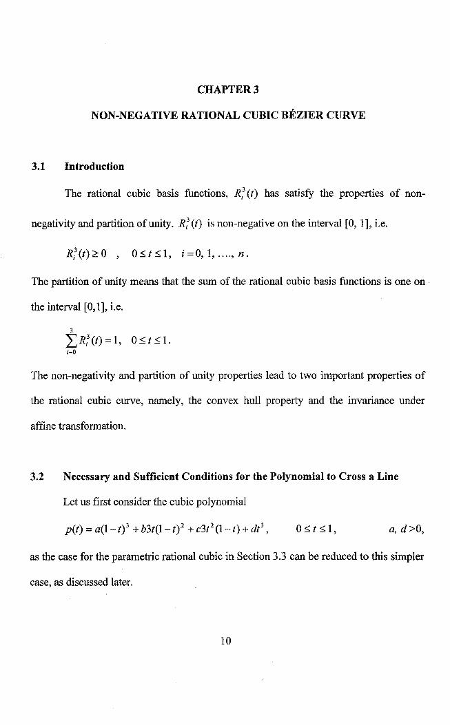
4.4.1 Case b < 0 and c ~ 0

In this case the inner Bezier point B lies on the other side of the given constraint

line but C does not. This case is shown at below in Figure 4.1. So we shall choose,u = 1,

i.e. the weight f3 is kept fixed while only a is being scaled.

A

Figure 4.1

D

the constraint line

Initial curve crossed the constraint line for case b < 0 , c~O.

21

We then require f(A) = 0 where

f(A) = (b 2c 2 - 4j3b3 d)A2 + (18aj3abcd - 4aac 3 )A - 27a 2 j3 2a 2d 2. (4.9)

Observe that when A = 0 ,

f(O) = -27a2 fJ 2a 2d 2 <0.

If f(l) < 0, then it means R(t) does not crosses over the line. According to Corollary

3.1, if R(t) crosses over the given constrained line, thenf(1) > O. By the Intermediate

Value Theorem, there exist A E (0,1) for whichf(l) = O. From (4.9), we observe that

when f(l) ~ 0 then

[(b 2c2 -4j3b 3d)1+(18aj3abcd -4aac3)] > 27a 2 j3 2a 2 d 2 > O. (4.10)

Ifwe consider the derivative of f(l) ,

1'(1) = 2(b2c2 -4j3b 3d)1 + 18afJabcd - 4aac 3

and compare to (4.10) then we get f'(l) > O. Hence fis increasing whenever f(l) ~ 0

on [0, 1]. This implies that f(A) has a unique positive root 1 in (0,1).

4.4.2 Case b ~ 0 and c < 0

This case is similar to Section 4.4.1 and it is shown in Figure 4.2. We shall

choose 1 = 1 and require g(p) = 0 where

g(fJ) = (b 2 c2 - 4aac3 )p2 + (18aj3abcd - 4j3b 3 d)p- 27 a 2 132 a 2 d 2

•

As Section 4.4.1, g(O) < 0, g(l) > 0 and g is increasing whenever g(fJ) ~ 0 on [0, 1].

Thus p to be the unique root of g in (0, 1).

22

A

D

the constraint line

c

Figure 4.2 Initial curve crossed the constraint line for case b ~ 0, c<O.

4.4.3 Case b < 0 and c < 0

In this case (see Figure 4.3), we shall scale both of the weights a and f3 by the

same scaling factor. Let Jl = /!, , we would require h( A) = 0 where

When /!,= 0,

and A = 1, R(t) crosses over the line then h(l) > O. Differentiate the h(A), we have

Observe that h'e/!') > 0, if /!, > O. Thus, h is increasing for /!, > O. By Intermediate

Value Theorem, there exist a unique root /!, E (0,1) of he/!') = O. We choose /!, to be the

23

unique root of h(}") = 0 in (0, 1). This value can be obtained by solving the equation

numerically.

Figure 4.3

B

Initial curve crosses the constraint line for case b < 0 and C<O.

4.5 Graphical Examples

D

We shall illustrate our discussion with five examples. The first three examples

are showing the cases in Sections 4.4.1, 4.4.2 and 4.4.3 respectively. The fourth example

is a closed curve with the arbitrary line as the constraint line, while last example shows a

closed curve with several constraint lines. In these examples, the data points are marked

by "0" and the two inner Bezier points of each curve segments are marked by "*". The

initial curve is drawn in dotted line form and the modified curve is drawn in full line

form. The corresponding data points of each example and the related scaiing factors are

given respectively in the following tables.

24

CONSTRAINED INTERPOLATION BY PARAMETRIC RATIONAL CUBIC...

Documents

Transcript of CONSTRAINED INTERPOLATION BY PARAMETRIC RATIONAL CUBIC...