Constitutive relations in dense granular flows

John J. Drozd and Colin DennistonDepartment of Applied Mathematics, The University of Western Ontario, London, Ontario N6A 5B8, Canada

(Dated: September 12, 2009)

We use simulations to investigate constitutive relations in dry granular flow. Our system iscomprised of poly-disperse sets of spherical grains falling down a vertical chute under the influenceof gravity. Three phases or states of granular matter are observed: a free-fall dilute granular gasregion at the top of the chute, a granular fluid in the middle and then a glassy region at the bottom.We examine a complete closed set of constitutive relations capable of describing the local stresses,heat flow, and dissipation in the different regions. While the pressure can be reasonably describedby hard sphere gas models, the transport coefficients cannot. In contrast to a hard sphere gas,transport coefficients such as viscosity and heat conductivity increase with decreasing temperaturein the fluid and glassy phases. The glass exhibits signs of a finite yield stress and we show that thestatic sand pile is a limit of our glassy state.

PACS numbers: 45.70.Mg,83.80.Fg,05.20.Dd

I. INTRODUCTION

The attempt to accurately describe stresses in granu-lar matter has a long history. The problem is difficultdue to the energy dissipation in the system that makesit hard for granular systems to achieve a true thermody-namic equilibrium. This makes the application of nor-mal equilibrium statistical mechanics techniques prob-lematic. Bagnold’s early work [1] on sheared granularsuspensions identified three different regimes of flow be-havior, the macroviscous dominated by the interstitialfluid, the transitional, and the grain inertia regime wherethe effects of the interstitial fluid are negligible (similarto dry cohesionless granular materials). Savage and col-laborators [2–5] worked to derive relationships based ona kinetic theory approach and describe things in terms ofa dimensionless parameter R which is the ratio of meanshear characteristic velocity to the r.m.s. velocity (ve-locity fluctuations). Durian and Menon [6] measured aclosely related quantity in a dry granular flow in a chuteand found that the velocity fluctuations were propor-tional to the mean flow velocity to the 2/3 power (i.e.δv ∼ v2/3) suggesting that R = v/δv may not be a natu-ral parameter for granular flows [7] as it is not likely to bea constant for any particular flow. Simulations indicatethat even the δv ∼ v2/3 is not true locally but is more astatement about global stress/energy balances (i.e. trueonly when suitably averaged over quite heterogeneous re-gions) [8]. This suggests a need to get measurements ofstresses, strains, and other transport phenomena on a lo-cal level, something that is ideally suited to simulationstudies.

The study of stresses and forces in static granular sys-tem has also been studied extensively. Force chain mod-els [9] demonstrated the wide distribution of forces ingranular packs. The consideration of the effects of di-rected force propagation suggests various constraints thatcan be placed on the stress tensor in granular packs [10–14]. Edwards and collaborators attempted to consolidatethese ideas on a statistical mechanics based on an av-

eraging over ensembles of mechanically stable packings[15, 16]. This, however, is predicated on the assumptionthat the distribution of mechanically stable packings ofspheres is relatively flat. There are suggestions that thismight not be the case [17]. It is therefore desirable togenerate configurations in a physically meaningful wayimplying a coupling between the dynamics responsiblefor creating static states (i.e. before it became static)and the static model itself is required. Thus simulationsof granular dynamics with a well defined static limit isdesirable.

Apart from adopting specific models, if we concentrateon the basic physics of momentum conservation, massconservation and energy conservation, this does not pro-vide us with enough equations to fully solve for localdensity, velocities, and temperature. In order to solvefor these quantities, the stress tensor and heat flux needto be expressed in terms of these local variables in orderto “close” the equations (i.e. have the same number ofequations and unknowns). This prompts us to studyingvarious constitutive relations to provide these necessaryadditional constraints. With this aim in mind, we haveperformed simulations of gravity driven dense granularflow in three dimensions to compare and test constitutivepressure, stress and energy relations of granular matter.

The binary, hard sphere collision model used for oursimulations is similar to that used in [8, 18], but for illus-trative purposes a typical snapshot from one of our sim-ulations is shown in Fig. 1(a). We will reiterate a briefdescription of our model in the next paragraphs but formore details one can refer to references [8, 18].

In our simulation, frictionless, rigid spherical grains aredropped in from the top of a rectangular chute and fallunder the influence of gravity. There are flat walls atthe left and right (x-direction) of the chute and periodicboundary conditions at the front and back (z-direction).At the bottom of the chute (y = 0), grains are reflectedwith a probability p (typically p = 90%). Particles trans-mitted through the bottom are replaced at the top of thechute in order to maintain steady-state. Particles reflect

2

ΠΡ

ΣΑΑ

FIG. 1: (a) Section of a simulation involving 43 200 grains with 15% polydispersity. The system size is 32a × 32a × 400a.There are reflective walls at x = 0 and x = Lx, periodic boundary conditions in the z-direction, and a finite probability ofreflection at the bottom of the chute (at y = 0) with an asymptotic coefficient of restitution µ0 = 0.97. Time-averaged density(volume fraction) in (b) and y− velocity in (c) down the center of a 3D chute. The short dashed lines are analytic calculationsof density and vy in the free-fall region (described in text). (d) The total kinetic energy E = 1

2ρv2 + 3

2ρT and (e) stress tensor

components σxx (solid line), σyy (dashed line) and σzz (dotted line). The measurements for plots (b), (c), (d) and (e) weretaken down the center of the chute.

off the walls of the chute with a partial loss, typically10% in their vertical (y) velocity. This is essential as ex-periments show [19, 20] that much of the column weightis supported by the walls.

Particles in our simulation undergo binary collisionswhere their momenta are transferred along the line join-ing their centers. Specifically, the velocities after collisionr′1 and r′2 in terms of the velocities before collision, r1 andr2, are

(r′1r′2

)=

(r1

r2

)(1)

+(1 + µ)

(m1 + m2)

( −m2 m2

m1 −m1

)(r1 · qr2 · q

)q,

where q = (r2 − r1)/|r2 − r1|, and µ is the coefficient ofrestitution. Such collision models of granular flow have along history [3, 5]. µ is a velocity-dependent restitutioncoefficient described by the phenomenological relation[21,22],

µ (vn) ={

1− (1− µ0) (vn/v0)0.7

, vn ≤ v0

µ0 , vn ≥ v0.(2)

Here vn is the component of relative velocity along theline joining the grain centers, µ0 is the asymptotic co-efficient at large velocities, and v0 =

√2ga [23]. Equa-

tion (2) effectively makes the ball collisions become moreelastic as the collisions become weaker as observed ex-perimentally [24, 25]. Scaled units are given in footnote

3

[26].In previous work [8, 18] we examined both mono- and

poly-disperse mixtures of spheres. Here we simulate onlysystems with 15% poly-disperse particles. In this context,a polydispersity of 15% means that the standard devia-tion of a particle radius is 0.15 if the mean is 1 usinga gaussian distribution of radii. Poly-disperse particlesachieve a truly glassy state, and here we are interested intesting and comparing constitutive relations in the glassystate, in addition to the free-fall and fluid states. Mono-disperse or nearly mono-disperse particles experiencingshear often increase in order and crystallize [8, 18, 27],and it is beyond the scope of this paper to examine theapproach to the crystallized state in detail, although wedid touch upon such details in previous work [8, 18].

A typical steady-state configuration of our simulationis shown in Fig. 1(a). The steady-state density (plot-ted as a volume fraction), velocity, energy, and diagonalstresses from our simulation for this typical configurationwere measured all down the center of the channel and areplotted in Figs. 1(b), (c), (d) and (e), respectively. Theorientation of the x, y and z axes is shown at the bottomof the visualization in Fig. 1(a).

As indicated by the labels and vertical dashed linesin Figs. 1(b)-(e), there are three regions, which we labelas a glassy region, a fluid region and a free fall region.These labels were justified in our previous work [8, 18].In the free fall region the grains accelerate at 1 g andcollisions do not have a significant impact on their kinet-ics [8, 18]. In the liquid region the density is sufficientlyhigh that collisions mix the grains, but the distributionof collision times are exponential, meaning that collisionsare largely independent. In the glass region, the collisiontime distribution is a power-law and thus collisions arenot independent and as a result there are collisions at awide range of time scales [18].

It is important to note that the relative sizes of theglassy, fluid and free-fall regions vary depending on thecoefficient of restitution used. As expected, the lowestasymptotic coefficient of restitution of 0.9 resulted in thesmallest fluid region, an intermediate asymptotic coeffi-cient of restitution of 0.95 resulted in a larger fluid re-gion, and the largest asymptotic coefficient of restitutionof 0.99 resulted in the largest fluid region for the samesized column. The existence of transition regions betweenthe free-fall, fluid and glassy states was demonstrated inprevious work [8]. The transition region between the free-fall region and the fluid region is indicated by the verticalgray shaded stripe in Figs. 1(b-e). Unless noted, the re-sults shown in this paper use an asymptotic coefficientof restitution of 0.97 so we can study one of the widertransition regions. A wider fluid region clearly shows akink in the free-fall to fluid transition region in the dataprofiles as shown in Figs. 1(b)-(e). It is interesting tonote that the kink at this transition in the density andvelocity profiles lines up with the peak in the kinetic en-ergy and inflection point in the stress profiles as shownin Figs. 1 (d) and (e). This peak marks the boundary be-

tween the fluid region and the free-fall to fluid transitionregion.

II. CONTINUUM EQUATIONS

Our simulation evolves over discrete binary collisions.In our simulation, we average various physical propertiesbased on these discrete events over time and space. Weresolve our 32a × 32a × 400a chute over a fine volumegrid composed of 1a×1a×1a cubes. This resolution waschosen to scale with the size of the particles of mean radiia = 1. This allows us to map our discrete system ontoa time-averaged continuum set of fields. We will nowbegin by describing the continuum equations describingthe average density, 〈ρ〉, velocity 〈~v〉 and energy 〈E〉 thatwe would expect our system to map onto. To simplifythe notation, even though the measured properties in oursimulation are quantities averaged in time and over thetranslational invariant z-direction, we omit the angledbrackets 〈·〉 in the conservation equations that follow.Typical averaging times are 600 to 1000 time units after200 time units of equilibration. The equilibration timeof 200 time units is equivalent to the typical lifetime of aparticle in the chute for the slower moving systems (i.e.the time from when it enters at the top to falls out thebottom).

A. Conservation equations

In this section, we will describe the continuum equa-tions of conservation of mass, momentum and energy thatwe will attempt to map our simulation results onto. Wewill describe how the physical terms in these equationscan be measured directly from our simulation.

The continuity equation for mass gives us one equation

∂ρ

∂t+∇ · (ρv) = 0. (3)

Momentum conservation requires that

∂t(ρvα) + ∂β(ρvαvβ) = ∂βσαβ + ρgα, (4)

where σαβ is the stress tensor, and all vα and vβ refer tofirst moments of the velocity distribution. This gives usthree Navier-Stokes equations.

The time averaged stress tensor can be directly mea-sured in our simulation using the microscopic form of the3D stress tensor [28]:

σαβ = σkineticαβ + σcollision

αβ (5a)

= −〈ρ (vα − 〈vα〉) (vβ − 〈vβ〉)〉 (5b)

+1t

∑

collisions

−12(1 + µ)(r1 − r2) · q (q · eα) (q · eβ) .

The 12 accounts for the double counting of collisions in

the sum (we count the transfer from particle 1 to 2 andthe transfer from 2 to 1).

4

Our fifth equation is an equation describing the energyconservation in our system

∂t (E) + ∂α (vαE + Fα) = I + ρg · v (6)

The (kinetic) energy is

E =12ρv2 +

32ρT. (7)

Note that v2 = 〈v〉2 in the first term and

T =13δv2 =

(〈v2

x〉+ 〈(vy − 〈vy〉)2〉+ 〈v2z〉

)/3 (8)

is the granular temperature. The energy, E, from oursimulation is plotted in Fig. 1(d). F is the non-convectiveenergy flux and α refers to the x, y or z component.

An important component of the non-convective energyflux F, is the collision energy flux, Fc. Part of the energyflux is related to the coherent transfer of momentum, thatis, the work done by the stress tensor and the other partis the heat flux. We can measure the energy transferedbetween grains in a collision using Eq. (1)[28] to get

δFc =1 + µ

m1 + m2

[m1 (r1 · q)2 −m2 (r2 · q)2

]q. (9)

Averaging over time gives the collision energy flux as

Fc =1t

∑

collisions

δFc. (10)

Similarly, we can easily use Eq. (1) to calculate thedissipation, I from the kinetic energy lost in each colli-sion,

δI = − 1− µ2

2(m1 + m2)(m1r1 · q−m2r2 · q)2 . (11)

If we average δI over the collisions that occur in a smallcell (1× 1×Lz) of our simulation, and if we also averageδI per unit time (effectively multiplying by the collisionfrequency fc), we arrive at the average dissipation rate Iwhich is the remaining term in Eq. (6).

Equations (3), (4) and (6) give us five equations (inthe static limit), but there are six unknown stress values,namely the diagonal stresses σxx, σyy, σzz, and usingthe fact that the stress tensor is symmetric, we have theshear stresses σxy = σyx, σxz = σzx and σyz = σzy.We need six constitutive equations to solve for these sixunknown stress values. Similarly, all the terms in Eq. (6)can be measured directly from a simulation, however theycannot be predicted ahead of time without relating theF and I to the density, velocities, or energy by means oftwo additional constitutive relations. The dissipation andheat flux will be examined in more detail in sections II Eand II G.

B. Stress and energy balance

In the previous section we described the conservationequations that are applicable to our system. In the up-coming sections we will examine these conservation equa-tions in detail applying them to the different regions ofour simulation. In this section we will examine the bal-ance of stress and energy in the fluid, glass and free-fallregions.

First examine Eq. (4) in the liquid and glassy regions.The stress tensor cannot be ignored in these regions, evenas a first approximation. If we assume in Eq. (4), that thetime derivative is zero as we are in steady state, and if weassume that the kinetic terms, ∂β (ρvαvβ) are negligible(as is observed by the low acceleration values in the glassyand in part of the fluid region in Fig. 2(c) in reference [8]and in Fig. 1(d) in reference [18]), we arrive at

∂xσyx + ∂yσyy = −ρgy, (12)

where gy = −g < 0 in this orientation.Figures 2(a) and (b) show the balance of the weight,

−ρg and stress gradients ∂xσyx + ∂yσyy in the fluid andglassy regions, respectively. There are very significantdifferences between how these terms are balanced in theliquid and glassy regions. We find that the pressure gra-dient ∂yσyy is the dominant term supporting the weightin the fluid region. This is consistent with what onewould expect in a simple fluid where the pressure wouldbe a function of depth, P = ρgy + constant. In contrast,in the glassy region we find that the gradient in the shearstress, ∂xσyx is the dominant term supporting the weight.Here, as in [18], we can conclude that in the glassy regionthe system supports a finite shear stress and this regionbehaves like a solid in this sense.

Now that we have looked at the stress balance in thefluid and glassy regions, we examine the balance in thefree-fall region. Taking the y component of the Navier-Stokes Eq. (4), we have

∂y

(ρv2

y

)= ∂yσyy + ρgy, (13)

where gy = −g < 0 in this orientation. Figure 2(c) showsthe balance of the weight, ρg and stress gradients ∂yσyy−∂y

(ρv2

y

). In the free-fall region the pressure gradient,

∂yσyy ≈ 0, and the kinetic term, −∂y

(ρv2

y

), contributes

solely to balance the weight, ρg.Finally, we explore the energy balance Eq. (6) in all

three regions. We can assume that the time partialderivatives are negligible since we are in steady state andthat the derivatives in the periodic z direction are alsonegligible. Note that the only significant energy fluxesare in the x and y directions and δv2

x ≈ δv2y ≈ δv2

z andthus we can say that T ≈ δv2

y (the isotropic assumptionis not strictly correct but is a reasonable first approxi-mation in the bulk regions [8]). Using these assumptionstogether with Eq. (6), we finally arrive at the energyequation

∇ · F = I + ρgvy, (14)

5

0.000

0.050

0.100

0.150fo

rce

dens

ityHaL

0.000

0.050

0.100

0.150

0.200

forc

ede

nsity

HbL

0 5 10 15 20 25 300.000

0.005

0.010

0.015

x

forc

ede

nsity

HcL

FIG. 2: Plot of force densities ∂yσyy (dot-dashed line), ∂xσyx

(long dashed line), ∂xσyx + ∂yσyy (short dashed line) andthe weight −ρgy (solid line) in (a) the fluid region and (b)the glassy region versus the width x for a 400-height columnusing an asymptotic coefficient of restitution µ0 of 0.97 andprobability of reflection p = 90%. (c) Plot of force densities∂yσyy (dot-dashed line), −∂yρv2

y (long dashed line), (∂xσyy −∂yρv2

y (short dashed line) and the weight −ρgy (solid line) inthe free-fall region.

where we have used the following relation to separate thekinetic and collision energy flux [4]

F = Fc − 12〈ρ (vα − 〈vα〉) (vβ − 〈vβ〉)〉vβ (15)

The left and right sides of Eq. (14), as directly measuredfrom our simulation, are plotted in Fig. 3. The clearagreement in the free fall, fluid and glass regions showsthat all the assumptions made to this point are reason-able.

Thus we see that particularly the stress balance distin-guishes the different states of the system but in order toactually solve the conservation equations we need to re-late the measured stress, dissipation, and energy flux tothe density, velocities, and granular temperature. Thisis the focus of the rest of the paper.

0 100 200 300 400-0.4

-0.2

0.0

0.2

0.4

y

Ñ×F

,I+Ρgv

y

FIG. 3: (a) Plot of the components of the energy equationfrom Eq. (14) in the free-fall region. The solid line is the leftside of the equation, ∇ · F, and the dashed line is the rightside of the equation, I + ρgvy.

C. Pressure

In our discussion of stress balance in the previous sec-tion, we demonstrated the role of the pressure gradient inbalancing the weight, particularly in the fluid and some-what less importantly in the glass. In this section, wewill examine several equations of state for pressure forthe glassy and fluid regions of our system. In a simplefluid the pressure is normally defined as

P = −13Tr (σ) , (16)

and the diagonal stresses σαα = −P . However, as isalready clear from Fig. 1(e) the diagonal stresses are notequal everywhere, so we will examine the pressure tensordiagonal components as

Pαα = −σαα. (17)

As jamming is approached, Salsburg and Wood [29]used a free volume approximation to suggest that thepressure in a classical (conservative) hard sphere systemapproaches

P = (ρT )(1− (φ/φc)1/D)−1, (18)

They also gave an asymptotic approximation (as φ → φc)of Eq. (18) as

P = D(ρT )(1− φ/φc)−1. (19)

In Eqs. (18) and (19) D is the dimension and φ is avolume packing fraction

φ =43πa3 ρ

m, (20)

where m is a mean grain mass, and φc is a random close-packed density. For monodisperse spheres, φc is knownto be ∼ 0.64. As our spheres are polydisperse φc is un-known and must be fit. Typically it is slighly lower than

6

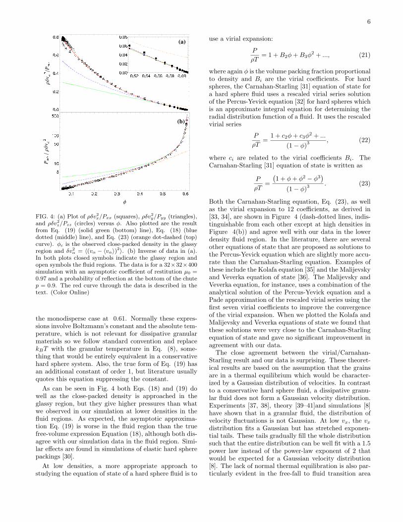
FIG. 4: (a) Plot of ρδv2x/Pxx (squares), ρδv2

y/Pyy (triangles),and ρδv2

z/Pzz (circles) versus φ. Also plotted are the resultfrom Eq. (19) (solid green (bottom) line), Eq. (18) (bluedotted (middle) line), and Eq. (23) (orange dot-dashed (top)curve). φc is the observed close-packed density in the glassyregion and δv2

α = 〈(vα − 〈vα〉)2〉. (b) Inverse of data in (a).In both plots closed symbols indicate the glassy region andopen symbols the fluid regions. The data is for a 32×32×400simulation with an asymptotic coefficient of restitution µ0 =0.97 and a probability of reflection at the bottom of the chutep = 0.9. The red curve through the data is described in thetext. (Color Online)

the monodisperse case at 0.61. Normally these expres-sions involve Boltzmann’s constant and the absolute tem-perature, which is not relevant for dissipative granularmaterials so we follow standard convention and replacekBT with the granular temperature in Eq. (8), some-thing that would be entirely equivalent in a conservativehard sphere system. Also, the true form of Eq. (19) hasan additional constant of order 1, but literature usuallyquotes this equation suppressing the constant.

As can be seen in Fig. 4 both Eqs. (18) and (19) dowell as the close-packed density is approached in theglassy region, but they give higher pressures than whatwe observed in our simulation at lower densities in thefluid regions. As expected, the asymptotic approxima-tion Eq. (19) is worse in the fluid region than the truefree-volume expression Equation (18), although both dis-agree with our simulation data in the fluid region. Simi-lar effects are found in simulations of elastic hard spherepackings [30].

At low densities, a more appropriate approach tostudying the equation of state of a hard sphere fluid is to

use a virial expansion:

P

ρT= 1 + B2φ + B3φ

2 + ..., (21)

where again φ is the volume packing fraction proportionalto density and Bi are the virial coefficients. For hardspheres, the Carnahan-Starling [31] equation of state fora hard sphere fluid uses a rescaled virial series solutionof the Percus-Yevick equation [32] for hard spheres whichis an approximate integral equation for determining theradial distribution function of a fluid. It uses the rescaledvirial series

P

ρT=

1 + c2φ + c3φ2 + ...

(1− φ)3, (22)

where ci are related to the virial coefficients Bi. TheCarnahan-Starling [31] equation of state is written as

P

ρT=

(1 + φ + φ2 − φ3

)

(1− φ)3. (23)

Both the Carnahan-Starling equation, Eq. (23), as wellas the virial expansion to 12 coefficients, as derived in[33, 34], are shown in Figure 4 (dash-dotted lines, indis-tinguishable from each other except at high densities inFigure 4(b)) and agree well with our data in the lowerdensity fluid region. In the literature, there are severalother equations of state that are proposed as solutions tothe Percus-Yevick equation which are slightly more accu-rate than the Carnahan-Starling equation. Examples ofthese include the Kolafa equation [35] and the Malijevskyand Veverka equation of state [36]. The Malijevsky andVeverka equation, for instance, uses a combination of theanalytical solution of the Percus-Yevick equation and aPade approximation of the rescaled virial series using thefirst seven virial coefficients to improve the convergenceof the virial expansion. When we plotted the Kolafa andMalijevsky and Veverka equations of state we found thatthese solutions were very close to the Carnahan-Starlingequation of state and gave no significant improvement inagreement with our data.

The close agreement between the virial/Carnahan-Starling result and our data is surprising. These theoret-ical results are based on the assumption that the grainsare in a thermal equilibrium which would be character-ized by a Gaussian distribution of velocities. In contrastto a conservative hard sphere fluid, a dissipative granu-lar fluid does not form a Gaussian velocity distribution.Experiments [37, 38], theory [39–41]and simulations [8]have shown that in a granular fluid, the distribution ofvelocity fluctuations is not Gaussian. At low vx, the vx

distribution fits a Gaussian but has stretched exponen-tial tails. These tails gradually fill the whole distributionsuch that the entire distribution can be well fit with a 1.5power law instead of the power-law exponent of 2 thatwould be expected for a Gaussian velocity distribution[8]. The lack of normal thermal equilibration is also par-ticularly evident in the free-fall to fluid transition area

7

(the low density region in Fig. 4(b)). Here the Pyy datamatches the Carnahan-Starling equation and the virialexpansion, but Pxx and Pzz do not. This indicates thatin this transition region, the fluid is not fully equilibratedin the x-x and z-z directions. Thus we shouldn’t expectthat Eq. (23) and the coincident virial expansion can bedirectly applied to a granular fluid. However, surprisinglythe Carnahan-Starling and the virial expansion work ex-tremely well in the fluid region, matching our simulationdata. A reason may be that even though in the veloc-ity distribution the 1.5 power law exists in the tails, thedistribution still remains Gaussian in the center. Thisimplies that the pressure in the fluid and free-fall regionis not too sensitive to the tail distribution.

It is also remarkable that there is no real signature ofthe different phases in the pressure. The ratio of P/(ρT )diverges as close packing is approached but is still finitethroughout the glassy region. As we shall see below,these phases are only distinct when we consider dynamicproperties such as transport coefficients. This fits withthe usual description of the glass transition being a dy-namical transition. What is perhaps more interesting isthat the free-fall to fluid transition must also be a dy-namic transition if these phases are truly distinct. Wewill examine this in more detail in later sections.

An asymptotically matched expression that interpo-lates between the virial and the free-volume expressionfor the pressure can be found by taking the virial expan-sion up to and including B5φ

4 and adding to it Eq. (18)and subtracting the Taylor series expansion of Eq. (18)taken about φ = 0 up to and including the φ4 term:

P

ρT= (1 + B2φ + B3φ

2 + B4φ3 + B5φ

4)

+

[1−

(φ

φc

)1/3]−1

−n=12∑n=0

(φ

φc

)n/3

. (24)

This is shown in Fig. 4 as the solid red line that goesthrough the simulation data.

D. Collision frequency

Many of the constitutive relations derived in followingsections, such as for the dissipation and energy flux, willinvolve a collision frequency (per unit volume). Thus, itseems appropriate to first establish closed relations forthe collision frequency, fc that are valid in the differentregions. As we will show below, a closed relation for thecollision frequency can be found from the expression 5 forthe stress measured in the simulation and the fact thatEq.(24) expresses the pressure in the different regions interms of the density and temperature.

We use the sign convention for the pressure tensorPαβ = −σαβ . The virial can be defined from the stress

à

à

à

à

0.95 0.96 0.97 0.98 0.99 1.001.4

1.5

1.6

1.7

1.8

1.9

2.0

Μ0

A

FIG. 5: Plot of the empirically determined parameter A inEq. (30) for the glassy region of the chute from simulationswith different asymptotic coefficients of restitution µ0. Theline is just a guide for the eye.

as

V = −13Tr (σαβ − 〈ρ (vα − 〈vα〉) (vβ − 〈vβ〉)〉) , (25a)

≈ P − ρT, (25b)

where the pressure P is a function of the density ρand granular temperature T as detailed in the pre-vious section. The kinetic term in Eq. (25a),〈ρ (vα − 〈vα〉) (vβ − 〈vβ〉)〉, is negligible in the glass butis significant in the fluid and free-fall regions.

Using Eq. (5) we also have the relation

V =12fc〈(1 + µ)(r1 − r2) · q〉,

= fc〈1 + µ〉〈vn〉, (26)

where

(r1 − r2) · q = vn (27)

is simply the normal impact velocity between the collid-ing particles and the factor of 1/2 disappeared becauseit was due to the double counting in the average overcollisions (which counts the momentum transferred fromparticle 1 to 2 and from particle 2 to 1 in) and this is notpresent in the second line.

By combining Eqs. (25a) and (26) we have

fc =3V

〈1 + µ (vn)〉〈vn〉 , (28)

µ (vn) is the velocity-dependent coefficient of restitutiongiven by Eq. (2).

During a collision the sign of vn is fixed and vn is al-ways positive, as can be readily seen from Eq. (27). InRef. [8], we showed that v2

n traces the velocity fluctua-tions δv2

α. Thus we expect 〈vn〉 to be related to 〈|δvα|〉,

〈|δvα|〉 =

√2π〈δv2

α〉1/2, (29)

8

if δvα is distributed in a Gaussian. This is nearly truein the liquid and free-fall regions. However, δvα is notstrictly distributed in a Gaussian distribution in theglassy region. If the particles are moving statisticallyindependently

〈vn〉 =

√2π

AT 1/2, (30)

where A = 2 in the liquid and free-fall regions. In theglassy region P (δv) is not Gaussian [8] and the particlesare not moving or colliding independently [8, 18]. So〈vn〉collisions 6= 〈δv〉particles. Thus in the glass, A < 2and a value for A has to be determined empirically. Foran asymptotic coefficient of restitution of µ0 = 0.97, wefound A = 1.62 in the glass. Figure 5 shows a plot ofA in the glassy region for three different coefficients ofrestitution. As the simulation becomes more elastic, thatis as µ0 → 1, A → 2.

We also calculated A in the glassy region for simula-tions with different sieve probabilities, hence for differentflow rates with the same asymptotic coefficient of resti-tution, and found that A did not vary with the flow ratein the glassy region.

Upon combining, Eqs. (2), (28), and (29), we finallyarrive at closed expression for the collision frequency fc,

fc =3V[

2− (1− µ0)(√

2π AT 1/2

v0

)0.7] √

2π AT 1/2

, (31)

with A as defined for the different regions in the para-graph above. We have used the fact that in the glassthe normal velocity, vn, is less than the cutoff velocityv0 =

√2ga [23]. Fig. 6 shows that the collision frequency

as calculated using Eq. (31), and the collision frequenciesobtained from the simulation agree nicely. To use thisexpression in one of the continuum relations, the virialV would need to be calculated using Eq.(25b) and (24)which give V in terms of density and temperature.

E. Conservation equations in free-fall region

In this section, we will examine properties in the free-fall region which we can solve for analytically. In thefree-fall region, the stresses are very small, and their gra-dients even smaller. As can be seen in the flat pressureprofile in the free-fall region in the inset in Fig. 1(e), thereis a small (mostly kinetic) stress contribution. This al-lows us to greatly simplify the above equations and solvefor the density, velocity and energy in the free-fall region.As described in Ref.[8], the fluid region starts as a bound-ary layer in the free-fall region which gradually grows todominate the flow. As such, what we describe in this sec-tion just applies to the plug-like flow in the central (awayfrom the walls) portion of the channel. In this plug-likeflow region, velocity gradients in the x-direction are neg-ligible (e.g. see Fig. 3(b) in Ref. [8]), as are shear stresses

ç

ççç ç ç ç

ç ç ç ç ç ç çççç ç ç

ç

ç

ç

ç

ç

çç ç ç ç ç ç ç ç ç ç ç ç

áááá á á á

á á á á á á áá á

á á áá

á

á

á

áá á á á á á á á á á á á á

50 100 150 200 250 300 350 4000

10

20

30

40

50

60

y

f c

HaL

ç

ç

ç

ç

ç

ç

ç

ç

ç

ç

çç

ç

ç

ç

ç

ç ççç ç

ç çç ç

ççç

ç

ç

ç

á

á

á

á

á

á

á

á

á

á

áá

á

á

á

á

á ááá á

á áá á

ááá

á

á

á

260 280 300 320 340 360 380 400

0.01

0.1

1

10

y

f c

HbL

FIG. 6: Plot of the collision frequency per unit volume ascalculated using Eq. (31) using A = 1.62 (red line with ◦’s),as calculated using Eq. (31) using A = 2 (purple line with¤’s), and the simulation values for the collision frequency(blue solid line) versus the height y of the chute in (a) theentire chute and (b) in the fluid region (semi-logarithmic).Measurements are taken in the center of the chute using asimulation with an asymptotic coefficient of restitution µ0 =0.97. (color online). Data is averaged over depth (32a) in zand over 800 time units.

σxy. Due to the periodic boundary conditions in the z-direction physical properties are translational invariant,on average, along z. Our system is in a steady state so wecan also assume that the partial derivative with respectto time in Eq.(3), (4), and (6) are negligible.

With these assumptions in the free-fall region, the Con-tinuity Eq. (3) translates to:

∂y (ρvy) = 0. (32)

and the y component of the Navier-Stokes Eq. (4) trans-lates to

∂y

(ρv2

y

)= ∂yσyy + ρg. (33)

There is a very small kinetic contribution to the stress ascan be seen in the inset in Fig. 1(e):

σyy = −ρδv2y. (34)

However this kinetic stress contribution in the free-fallregion is nearly constant (except close to the inlet) as canbe seen by the horizontal profile in the inset in Fig. 1(e),and thus

∂yσyy = −∂yρδv2y ≈ 0. (35)

9

We can then solve for the density and velocity in thefree-fall region using Eqs. (32) and (33) and one datapoint in the bulk interior of the free-fall region at a heighty0, at mid-width (mid x−direction) and mid-depth (midz−direction) in the chute. The reason we use an interiorpoint as opposed to a boundary value, say at the top ofthe chute is because the assumption of σyy being constantis most true once the grains have moved a finite distanceinto the chute. This is not strictly a required assumptionto solve the equations, but it is required if we wish tosolve without consideration of the energy equation.

Thus solving Eqs. (32) and (33), gives us the solution

ρ = c/vy, (36)

vy ≈ −√

2gy + k1, (37)

where the constants are

k1 = v2y0− 2gy0, (38)

c = ρy0vy0 , (39)

where ρy0 and vy0 are from any single point in the interiorof the free-fall region as described in the previous para-graph. Eqs. (37) and (36) are plotted as dashed linesin the free-fall region in Fig. 1(b) and (c). The agree-ment between the analytical results and the simulation inthe free-fall region is remarkably good. Not surprisingly,there is some deviation at the very top of the chute wherethe approximation that σyy ≈ constant breaks down. Aswe noted above, in the free fall region the stress is almostentirely from the kinetic terms so that σyy = −ρδv2

y soto improve our analytic solution we must examine theenergy equation (to obtain a better solution for δv2

y).It is clear however, that to solve these equations an-

alytically (or numerically without input from the sim-ulation) that constitutive relations giving I and Fc areneeded. These will be presented in section II G.

F. Shear-Stress Constitutive Relations: Models ofViscosity

In references [8] and [18], it was demonstrated thatthe velocity profile of particles in the fluid region wasparabolic (Poiseuille flow), but as one approached theglassy region a plug type profile emerged. The devel-opment of this plug profile in the y-velocity was clearlycorrelated with the center region solidifying into a glass.As the particles travel down the chute, they are slowedby the drag force at the walls supporting the weight ofthis glassy region via a shear stress. This gives a plug-like profile. We cannot overemphasize the important rolethat the shear stress has on the y-velocity profiles forparticles traveling from the fluid to a glassy region. Thestresses were shown to be crucial in providing the weightbalance that we discussed in section II B. In this section,we will discuss constitutive relations for the shear stressin the fluid and glassy regions of our granular system.

Most works based on kinetic theory assume a fluid-likeconstitutive relation for the shear stress in the system

σxy = η∂xvy, (40)

where σxy is the shear stress, η is the effective viscosityand ∂xvy is the shear rate. The difficulty with such de-scriptions is that the viscosity η is strongly dependent onthings like the granular temperature which varies consid-erably in space in many granular systems.

This complexity can be seen in Fig. 7(a) which plotsthe shear stress, σxy, vs. the shear rate ∂xvy in the gran-ular fluid region for different heights. Here, it was impor-tant to use a slow (p = 90%) system with a high enoughasymptotic coefficient of restitution µ0 = 0.95 in orderto achieve a true fluid region of study. The temperaturein this region is fairly uniform in width x but changesdramatically in height y (see Figs. 5 and 6 in reference[8]). We plotted the shear stress σxy versus the shearrate ∂xvy for different heights, hence at different temper-atures for these different heights, as shown in Fig. 7(a).Fig. 7(a) does display the linear relation of Eq. (40). Tocalculate the viscosity η, we then measured the slopes ofσxy versus ∂xvy at these different heights, and plottedthese viscosity values versus the granular temperature Tat these heights. We obtained a power-law relationshipbetween the viscosity and the granular temperature alongheights in the fluid region as shown in Fig. 7(b).

η ∼ T−4/3. (41)

Equation (41) for the fluid region seems surprising. If yourecall, in section II C, particularly by looking at Fig. 4,we were able to successfully match the pressure in thefluid region from our simulation to the pressure equationof state obtained from a virial expansion. Thus it wouldbe logical that one should expect our fluid to behave as ahard sphere gas whose viscosity as given from any stan-dard textbook [42] would be:

η =564

1a2

√mkBT

π, (42)

where a is the particle radius, m its mass, kB is Boltz-mann’s constant and T is the absolute temperature. Onecan see from Eq. (42), for a hard sphere gas, the viscos-ity η ∼ T 1/2. Thus one would expect the viscosity to in-crease with temperature, but from Eq. (41) and the corre-sponding Fig. 7(b), the viscosity actually decreases withincreasing temperature. This is not how a gas behaves.This behavior is often associated with a liquid whose vis-cosity grows larger as the temperature goes down as youapproach the solid state. The viscosity in a liquid typi-cally has an exponential relation that is found in standardtextbooks [42]

η = η0eEa,η/RT , (43)

which as in our simulation data, does decrease with in-creasing temperature. In Eq. (43), Ea,η is the molar acti-vation energy. The fact that we observe a power relation

10

given by Eq. (41), and not the exponential relation givenby Eq. (43), indicates that our granular fluid is not a trulyequilibrated fluid. The data in Fig. 7(b), however, whenplotted on a semi-logarithmic scale (Fig. 7(c)), seems tobe approaching a straight line at higher temperatures(near the top of the fluid region), but not the 1/T sug-gested by Eq.(43).

Numerous experiments have measured velocities andforces in sheared granular matter [1, 43–45] confininggranular matter in a Couette cell between a stationaryouter cylinder and a rotating inner cylinder. These ex-periments are typically shearing a very dense granularstate like our glass. In Ref. [46], the authors looked atthe relationship between the square root of the granu-lar temperature and shear rate that was observed in theglassy region of granular particles in a Couette cell. Ourgranular particles are in a shear flow traveling down thechute. The shear zones near the walls in the glassy stateof our simulation should be comparable to these experi-ments.

Following the analysis given in reference [46], usingσxy = ηγ with γ = ∂xvy being the shear rate and ηthe viscosity, an expression was made for the viscosity toscale with the collision frequency,

η = η0P/(ρcd

2T 1/2)

, (44)

where d is the particle diameter, η0 is a dimensionlessnumber, and ρ ∼ ρc the close-packed density has beenassumed, so that

T 1/2 = η0P/(ρcd

2σxy

)γ. (45)

However, this analysis can be taken further. If the pres-sure given in Eq. (44) followed the scaling P ∼ ρT , thiswould give the same scaling η ∼ T 1/2 as Eq. (42) for ahard sphere gas. This extension was not done in Ref.[46]. The analysis that was provided by the authors inRef. [46], resulting in Eq. (45), gives γ = ∂xvy ∼ T 1/2.Their analysis did not lead to agreement with their ex-periment. Experimentally, they observed the followingpower-law with

T 1/2 ∼ |∂xvy|0.4 (46)

A log-log plot of the square root of the granular tempera-ture vs shear rate as measured from our simulation on oneside of the chute (from middle to the wall) in the glassyregion is shown in Fig. 8(a). We plotted this for a seriesof systems with different probabilities of sieve reflection,p and different asymptotic coefficients of restitution µ0.On a log-log plot the top curve in Fig. 8(a) vaguely re-sembles a power-law exponent of 0.4 as in experiment[46] for a fast system (p = 1%, µ0 = 0.9), and as shownby the superimposed bottom curves in Fig. 8(a), for theslower systems (p = 90%) with µ0 = 0.9, 0.95, 0.96 and0.97, the slope is 0.2, although this isn’t as clear a linearregime on a log-log plot of the square root of the granu-lar temperature (velocity fluctuations) vs. the shear rate

ò

òòòòòò

òò

ò

òòòòòò

ò

òò

òòòòòò

ò

àààààààààààààààààààààààààà

ææææææ æ

ææ

æ æææ æ

æææ

æææ æ

æææææ

ììììì ì

ìì ìììììììì ì

ì ììì ìì

ììì

-0.2 -0.1 0.0 0.1 0.2-0.2

-0.1

0.0

0.1

0.2

¶xvy

Σxy

HaL

ççççççççççççççççççççç

çç

ç

¨ ¨ ¨ ¨ ¨ ¨ ¨ ¨ ¨ ¨¨¨¨¨¨¨ ¨¨¨¨

õõ õõõõ

õõõõõõõõõõõõõõõõõõ

10.05.0 20.03.0 15.07.0

0.1

0.2

0.5

1.0

2.0

5.0

T

Η

HbL

ç

çççççççççççççç ç

ççç ç

ç

çç

ç

¨¨¨¨¨¨ ¨ ¨ ¨ ¨ ¨ ¨ ¨ ¨ ¨ ¨ ¨ ¨¨¨¨¨¨¨

õõõõõõõõõõõõõõõõõõõ

õõõõõ

5 10 15 20 25

0.1

0.2

0.5

1.0

2.0

5.0

T

Η

HcL

FIG. 7: (a) Shear stress σxy versus shear rate ∂xvy in thefluid region for a slow flow (probability of reflection at thebottom sieve of p=90%, µ0 = 0.95). The symbols indicatedata at different heights in the fluid region (N’s at y = 277,¥’s at y = 283, •‘s at y = 289 and ¨’s at 295), (b) Log-logplot of viscosity and (c) semilogarithmic plot of viscosity inthe fluid region (slope of data in (a)). The symbols indicatedifferent asymptotic coefficients of restitution, µ0 (with ◦’susing µ0 = 0.95 and p = 90%, ¦’s using µ0 = 0.96 and p =90%, and O’s using µ0 = 0.97 and p = 90%). Systems withthe higher asymptotic coefficients of restitution of µ0 = 0.95,0.96 and 0.97 achieve a true fluid region and have a consistentpower-law of − 4

3.)

for the slower systems as for the faster system. Thusthe power law exponent of 0.4 that was reported in theexperimental paper [46] is not universal.

Eq. (46) indirectly assumes that the viscosity in thesheared glass is a function of the granular temperature.Using the relation σxy = η∂xvy, we can plot the viscos-

11

óóóóóóóó

óó

óóóóó ó óóóóóóóóóóó

áááááá

áá

ááááá á á áá áááááááááá

çççççççççççççç çç ç ççç ç ç ç

ççççííííííííííííííí íí í í í

ííí íííí

0.001 0.01 0.1 1

0.5

1.0

2.0

¶xvy

T1�

2HaL

ó

óóóóóóóóóóóóó

áááááááááá

áá

ççççççççççç

ç

íííííííí

ííí

í

0.1 0.5 1.0 5.0 10.0 50.0

1020

50100200

5001000

T

Η=Σ

xy�¶

xvy

HbL

FIG. 8: (a) Log-Log plot of square root of temperature versusshear rate. A system with a fast flow (probability of reflectionat the bottom sieve of p = 1%,4 and µ0 = 0.9) yields a regionwith the experimental power law exponent of 0.4 (line), whileslow systems (probability of reflection at the bottom sieveof p = 90% with µ0 = 0.9 ¤, µ0 = 0.95 ◦, µ0 = 0.96 ¦, andµ0 = 0.97 O) have a pseudo-power-law with exponent 0.2. (b)Log-log plot of effective shear viscosity η = σxy/∂xvy versustemperature T in the glassy transition region for a fast flow(4) and slower flows (symbols same as in (a)). The solid lineshave slopes of -1.1 for the fast system, -2.3 for the slow systemwith µ0 = 0.9, and -2.8 for the slow systems with µ0 = 0.95,0.96 and 0.97.

ity, η as σxy/∂xvy, versus the granular temperature, T ,in the glassy region for both a slow (p = 90%) systemyielding a power law of 1.1 and a fast (p = 1%) systemyielding a power law of 2.3. This is shown as a log-logplot in Fig. 8(b). Clearly, the power-law exponent is notuniversal here.

We can however obtain a universal power law in thesheared glass by plotting the shear stress, σxy, vs. theshear rate, ∂xvy, on a log-log plot as shown in Fig. 9. Wefound a universal power law of 0.4 for both slow and fastsystems on one side of the chute:

σxy = B|∂xvy|0.4, (47)

with B a constant. This is equivalent to obtaining auniversal power law by further plotting (not shown) theviscosity, η on one side of the chute in the glassy regionversus the shear rate, γ = ∂xvy and witness a universalpower law of approximately −0.6:

η = B|∂xvy|−0.6 (48)

The universal power-law between the shear stress and

óóóóóóóóó

óó

ó

ó

ó

ááááááá

ááá

áá

á

á

ççççç

çççç

çç

ç

ç

ç

¨¨¨¨¨¨¨¨¨¨

¨¨

¨

¨

õõõõõ

õõõõ

õõ

õ

õ

õ

òòòòò

òòòò

òò

ò

ò

ò

0.001 0.01 0.1 1

0.1

0.2

0.5

1.0

2.0

5.0

10.0

¶xvy

Σyx

HaL

á

á

áááá

0.0 0.1 0.2 0.3 0.4 0.5 0.60.5

1.0

1.5

2.0

Hvy Lx�2 - vy wallL�HLx�2L

ΣyxÈ

wal

l

HbL

ΣY�

FIG. 9: (a) Log-log plot of shear stress σyx versus shear rate∂xvy in the glassy region for various flow rates (probability ofreflection at the bottom sieve of p=0.01 as 4’s, p=0.1 as ¤’s,p=0.25 as ◦’s, p=0.5 as4’s, p=0.75 as O’s, and p=0.9 as N’s),all with an asymptotic coefficient of restitution of µ0 = 0.9.The solid straight lines have slopes of 0.41 for the upper lineand 0.38 for the lower line. (b) Plot of shear stress σyx at thewall versus the y velocity at the center at Lx/2 minus the yvelocity at the wall, scaled by Lx/2. The yield stress σY isindicated by the arrow. Data is from a 32× 32× 250 column.

strain rate given by Eq. (47) and shown in Fig. 9(a)makes one wonder whether we have a true glassy region.Consider in Fig. 9(a) a typical region where a particleof radius a undergoes a strain rate ∂xvy of 0.01. In thisregion, vy ∼ 1 so using the relation

∂xvy =∆v

a, (49)

we can say that it takes 100 time units for one grainto pass another. However, using the typical size andvelocities from Fig. 1 the time that a particle has in theglassy portion of the chute is

Ly

vy≈ 200

1= 200 time units. (50)

Thus, in our glassy region, it takes about the sameamount of time for one grain to pass another as it takesfor all the particles to traverse the entire chute. It is alsoclear from Fig 9(a) that Eq.(47) is not valid all the wayinto the interior (low strain-rate region) of the systemand significant deviations occur below σxy . 0.4. An-other significant caveat is that we have taken the strain

12

rate ∂xvy as the derivative of the time averaged velocityprofile. While the time-averaged profile is smooth, an in-stantaneous velocity profile is much more discontinuous(so much so that one cannot meaningfully take a numer-ical derivative) suggesting more discrete fault-like slipsoccurring in the glass rather than the local rearrange-ments typical of a fluid.

If we look at the plot of shear stress at the wall (ex-perimentally measurable shear stress) versus the scaled yvelocity at the center minus the y velocity at the wall (ex-perimentally observable strain rate) shown in Fig. 9(b),we do observe a finite shear stress when the scaled y ve-locity at the center minus the y velocity at the wall iszero. This indicates that our glassy region has a yieldstress at this zero velocity as would be expected for aglassy region. Doing the same thing in the fluid region(not shown) shows a 0 intercept at small strain rates in-dicating the lack of a yield stress there. A constitutiverelation for the static central portion of the glass is stillneeded as we have only really described the shear zonesnear the wall in this section. We will consider this inmore detail in Section II H.

It is interesting to note that in no region do we observethe Bagnold scaling [1] of

σxy ∼ (∂xvy)2. (51)

However, Bagnold did not measure the shear stress orstrain rate locally but rather deduced them from the ex-ternally applied stress and strain in a Couette cell. Thisis more similar to our analysis in Fig. 9(b) which doesexhibit this quadratic relationship. However, our simula-tion is more akin to Poiseuille flow rather than Couetteflow so a direct comparison is not necessarily valid. How-ever, it does raise the possibility that Bagnold scaling is,similar to the relationship between δv and v found byMenon and Durian [6, 8], not a local relationship buta statement about a more global force/energy balance.However, simulations in the Couette geometry would beneeded to comment further on this aspect. Simulationsusing Hertzian contact types of interactions have seenregions of Bagnold scaling [47]. However, these simula-tions found that in the regions where Bagnold scalingwas obverved transmission of stresses was dominated bycontacts rather than collisions. It is possible that theaddition of tangential dissipation (i.e. friction) during acollision would be key to seeing Bagnold scaling but, if so,would not be consistent with Bagnolds original argumentwhich was based on binary collisions.

G. Energy equation

In section II A, the energy conservation during steady-state was expressed as

∂t (E) + ∂α (Fα) = I + ρg · v. (52)

In this section, we will examine the energy flux F and thedissipation I and relate them to the density and temper-

ature. We assume that the time derivative, ∂tE is zerobecause we are in steady state. We will focus first on theenergy flux F.

As stated in [28], there is a difference between the “en-ergy flux”, F, and the “heat flux”, Q. The heat flux, Qis the uncorrelated part of the energy flux, and can befound using

Q = Fc + (σ · v) , (53)

where Fc is the collision energy flux defined by Eq. (10)and σ is the stress tensor defined by Eq. (5). InEq. (53), σ · v represents the coherent transfer of energy(i.e. non-dissipative) during collisions.

Fourier’s law suggests that the heat flux across thechute, Qx, can be expressed as proportional to the gra-dient of the granular temperature, T , by the relation

Qx = −κ∂xT (54)

where κ is the thermal conductivity. In our fluid region,we plotted the heat flux, Qx versus the gradient of thegranular temperature, ∂xT , across the width (x direc-tion) of the chute. This is shown in Fig. 10(a) for a slowsystem using a probability of reflection at the bottomsieve of p = 90% and an asymptotic coefficient of resti-tution of µ0 = 0.95. Systems with higher coefficients ofrestitution had the largest fluid regions. It was impor-tant here to choose a system with a high asymptotic co-efficient of restitution in order to maintain a true fluid re-gion. Otherwise with lower coefficients of restitution, wewould have just a combination of fluid to glass and fluidto free-fall transition regions. As one can see for variousheights in the fluid region, the data in Fig. 10(a) falls onstraight lines. The negative slopes of these straight linesgive the thermal conductivity

κ = − Qx

∂xT. (55)

In Fig. 10, the thermal conductivity, κ was calculated as alinear fit and is shown on a semi-logarithmic plot versusthe granular temperature at a range of heights in thefluid region for three slow systems (p = 90%). Fig. 10shows systems with different asymptotic coefficients ofrestitution of µ0 = 0.95 shown as ¤’s, 0.96 shown as ◦’sand 0.97 shown as O’s. Interestingly, all three systemsconsistently give an exponential fit in the fluid region of

κ = Ae−T/T0 , (56)

where T0 ∼ 11, and A is a multiplicative constant.We can contrast Eq. (56) to a thermal conduction ex-

pression for a hard sphere gas given in reference [42]

κ =25128

cv

a2

(kBT

πm

)1/2

, (57)

where cv is a specific heat and a is the particle radius.It does not really make sense for our granular gas to

13

òò òòò

ò

ò

ò

ò

ò

ò

ò

ò

ò

ò

òòò òò

ààà

à

à

à

àà

à

à

à

à

àà

à

à

à

ààà

ææ æ æ æ æ

æ

æ

æææ

æ

æ

æ

æ æ æ æ ææ

ìììì

ìì ì ìììììì ì ìì

ìììì

-0.3 -0.2 -0.1 0.0 0.1 0.2 0.3

-20

-10

0

10

20

-¶xT

Qx

HaL

áááááááá á á á

áááááááááááá

á

á

á

á

á

çõçõçõçõçõçõçõçõçõçõçõçõçõçõçõçõçõçõçõçõçõçõ

çõçõçõçõçõçõçõ

çõ

çõ

çõ

ááááááááááááááááááá ááá á á

ááááá á á

áá ááááááááááá

á

á

0 5 10 15 20 25 301

510

50100

5001000

T

Κ

HbL

FIG. 10: (a) Heat flux Qx versus granular temperature gradi-ent, −∂xT , in the fluid region (probability of reflection at thebottom sieve of p=90%, µ0 = 0.97). The symbols indicatedata at different heights in the fluid region (N’s at y = 274,¥’s at y = 284, •‘s at y = 294 and ¨’s at y = 304), (b)Semi-logarithmic plot of thermal conductivity, κ = −Qx/∂xTversus the granular temperature, T , in the fluid region forsystems with a probability of reflection at the bottom sieveof p=90%. The symbols indicate different asymptotic coeffi-cients of restitution, µ0. (with ¤’s using µ0 = 0.95, ◦’s usingµ0 = 0.96, and O’s using µ0 = 0.97). All three systems give

an exponential fit of κ ∼ e−T/T0 with T0 ∼ 11.

have a specific heat as we potentially could argue for aninfinite specific heat for our dissipative simulation (anyenergy added to the system is eventually dissipated).From the equation for the thermal conductivity of a hardsphere gas given by Eq. (57), one gets the impression thatκ ∼ T 1/2 and thus that the thermal conductivity shouldincrease with temperature. The thermal conductivity forour granular fluid does not increase with temperature,but exponentially decays with increasing temperature asgiven by Eq.(56). Thus once again our granular fluid can-not be considered as a hard sphere gas. Our fluid behavesas a liquid: as the temperature goes down, the thermalconductivity increases as you would expect in a materialthat approaches a solid state as our glassy region.

Next, we examine the thermal conductivity in theglassy region. The heat flux, Qx is plotted in the glassyregion in Fig. 11 across the width (x direction) of the

-15 -10 -5 0 5 10 15

-20

-10

0

10

20

x

Qx

FIG. 11: Log-log plot of heat flux Qx = −κ∂x3T vs. widthx for a 15% polydisperse 3D simulation for a glassy regionat y = 200 where κ = 4/3πa3ρfc. The solid line is Qx =Fcx + σxyvy, and the dashed line is Qx = −4/3πa3ρfc∂x3T .

chute. As shown in Fig. 11, in the glassy region

κ = 3φfc =43πa3ρ3fc, (58)

(the density times the collision frequency). Eq. (58) is thesame equation as in reference [28] found in 2D where wemeasured density there as a volume fraction [48]. As thecollision frequency is known in terms of the density andtemperature (section II D) this gives a closed expressionfor the conductivity in the glass.

The remaining term for which we need a constitutiverelation is the dissipation, I. Since the coefficient ofrestitution µ, is highly correlated with the impact ve-locity vn, we cannot simply factor the terms in Eq.(11),− 1

4 〈(1 − µ2)v2n〉 as − 1

4 〈1 − µ2〉〈v2n〉 (we could factor out

(1 + µ) in previous expressions, such as for the collisionfrequency, because the relative change in (1+µ) for differ-ent vn is small whereas the relative change in (1−µ2) fordifferent vn is large). We outline below two different con-stitutive relations for I based on different assumptions.

In the first case, we assume that dissipation is dom-inated by the high impact collisions. We consider asmall proportion, say b, of the dissipation involves vn

being greater than the cutoff velocity v0 in our velocity-dependent coefficient of restitution Eq. (2), and a pro-portion 1 − b of the dissipation involves vn < v0. Thenwe have

〈δI〉 = 〈−14(1− µ2)v2

n〉 (59)

= b〈−14(1− µ2

0)v2n〉vn>v0

+ (1− b)〈−14(1− µ2)v2

n〉vn<v0 .

14

Now, for vn < v0

〈−14(1− µ2)v2

n〉vn<v0 ≈ 0, (60)

because µ ≈ 1 and vn is also small for these collisions.Similarly, the small value of vn for collisions with vn < v0

gives

〈v2n〉all = b〈v2

n〉vn>v0 + (1− b)〈v2n〉vn<v0 ,

≈ b〈v2n〉vn>v0 . (61)

Putting it all together gives

〈δI〉 =14(1− µ2

0)〈v2n〉. (62)

This is the expression we expect to be correct if highvelocity impacts dominate the dissipation.

However, most collisions occur with vn < v0 (althoughthese collisions are less dissipative so they may, or maynot, impact the total dissipation I). If the coefficientof restitution formula for vn < v0 is used directly andsubstituted into Eq. (2) and the average of the entireexpression is evaluated one gets

〈δI〉 =12

(1− µ0)v0.70

〈v2.7n 〉 − (1− µ0)2

4v1.40

〈v3.4n 〉. (63)

One can relate the averages of 〈v2.7n 〉 and 〈v3.4

n 〉 to 〈v2n〉

similar to Eq.(29). The total dissipation can be found as

I = 〈δI〉fc, (64)

with fc given in terms of density and temperature asdescribed in Section IID.

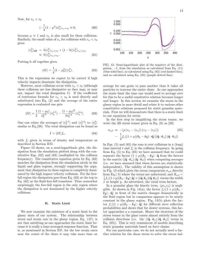
Figure 12 shows, on a semi-logarithmic plot, the dis-sipation from the simulation plotted along with the con-stitutive Eqs. (62) and (63) (multiplied by the collisionfrequency). The constitutive equation given by Eq. (62)matches the dissipation from the simulation nicely in theliquid and glass regions, strongly supporting the argu-ment that dissipation in these regions is completely domi-nated by the high impact velocity collisions. For the free-fall region the dissipation goes from Eq. (63) at the top toEq. (62) at the fluid-free-fall transition. Thus, somewhatsurprisingly the free-fall region is the only region wherethe dissipation is not dominated by the higher velocitycollisions.

H. Static Limit

We now examine the existence of a static limit to theglassy state of our system. The relationship betweenstress and strain rate in the glassy region, Eq. (47), isnot that satisfying as one approaches the static limit be-cause it is really a time-averaged response function. Thatis, as mentioned in Section II F, for the low strain ratesnear the center of the chute it may take more time on

100 150 200 250 300 350 4000.001

0.0050.010

0.0500.100

0.5001.000

y

-I

FIG. 12: Semi-logarithmic plot of the negative of the dissi-pation, −I, from the simulation as calculated from Eq. (11)(blue solid line), as calculated using Eq. (62) (red dashed line),and as calculated using Eq. (63) (purple dotted line).

average for one grain to pass another than it takes allparticles to traverse the entire chute. As one approachesthe static limit the time one would need to average overfor this to be a useful consitutive relation becomes longerand longer. In this section we examine the stress in theglassy region in more detail and relate it to various otherconstitutive relations proposed for static granular mate-rials. First we will demonstrate that there is a static limitto our equations for stress.

In the first step to simplifying the stress tensor, wewrite the 3D stress tensor given in Eq. (6) as [28]:

σαβ ≈ −〈ρ (vα − 〈vα〉) (vβ − 〈vβ〉)〉 (65)

− 12fc〈(1 + µ)(r1 − r2) · q〉〈(q · eα) (q · eβ)〉

In Eqs. (5) and (65) the sum is over collisions in a (long)time interval t and fc is the collision frequency. In goingfrom Eq. (5) to Eq. (65) we have assumed that we couldseparate the factor (1 + µ)(r1 − r2) · q from the factorsin the matrix 〈(q · eα) (q · eβ)〉 when computing averages(i.e. we have assumed that these factors are statisticallyindependent). The validity of this assumption is shownin Fig. 13 which plots the stress components σαβ directlyfrom Eq.( 5) where the terms are unfactored, and Rαβ =12fc〈(1+µ)(r1− r2)·q〉×〈(q·eα)(q·eβ)〉 versus the widthx or height y. As advertised, the virial term factors.

In a granular glass the kinetic term, 〈ρvαvβ〉 is negli-gible. As shown in Fig. 14(a), the factor fc〈(1 + µ)(r1 −r2) · q〉 in front of the matrix changes dramatically inthe fluid region but in comparison appears to be nearlyconstant in the glassy region. Fig. 14(b) plots the fac-tor fc〈(1 + µ)(r1 − r2) · q〉 for different sieve reflectionprobabilities and shows that for slower systems, this fac-tor approaches a a constant. Hence the structure of thestress tensor in the glass comes almost entirely from thecollision directions (i.e. the 〈(q · eα) (q · eβ)〉 terms inEq. (65)). This is very reminiscent of models describingstatic granular materials based on force chains.

For our particular case, we do not actually need a fur-ther relation for the shear stress to solve the stress bal-

15

ç

ç

ç

çç

çççççççççççççççççççççç

ç

ç

ç

ç

ç

5 10 15 20 25 30-2.0

-1.0

0.0

1.0

2.0

x

Σxy

,Rxy

HaL

ççççççççççç

ççççç

ç

ç

ç

ç

ç

ççççç

á

áááááá

áááááááááá

á

á

á

á

ááááá

óóóóóóóóóó

óóóóóóó

ó

ó

ó

ó

óóóóó

ççççççççççç

ççççç

ç

ç

ç

ç

ç

ççççç

á

áááááá

áááááááááá

á

á

á

á

ááááá

óóóóóóóóóó

óóóóóóó

ó

ó

ó

ó

óóóóó

0 100 200 300

-10

-8

-6

-4

-2

0

y

ΣΑΑ,RΑΑ

HbL

FIG. 13: Shear stress σxy (solid line) and Rxy (circles)(righthand side of Eq. (65), the shear stress factorized into the col-lision directions, 〈(q · x) (q · y)〉 and the constant − 1

2fc〈(1 +

µ)(r1 − r2) · q〉) versus x in (a) the glassy region at a height,y = 100. (b) Plot of the diagonal stress, σαα with its ki-netic term (lower curves) and without its kinetic term (uppercurves), and factor Rαα versus height y. (σxx is the solidline, σyy is the dashed line, and σzz is the dot-dashed line,Rxx is circles, Ryy is squares, and Rzz is triangles). Datais for a 400-height column using an asymptotic coefficient ofrestitution µ0 of 0.97 and a probability of reflection, p = 0.9.

ance Eq. (12). As ∂yσyy ≈ 0 in the glassy state, it isclear that σxy ≈ ρgx + constant. Making use of sym-metry about the center (x = 16) of the chute, it followsthat the constant should be −ρg16. However, this is re-ally just a statement about stress balance in the systemand requires the a-priori assumption of the shear stresssupporting the weight. In order to compare to other con-stitutive relations suggested for static granular materialsit is worthwhile to decompose the stress/pressure tensorinto its eigenvalues Λi and eigenvectors n, m, and l :

pαβ = −σαβ = Λ1nαnβ + Λ2mαmβ + Λ3lαlβ . (66)

Note that the stress tensor is real, symmetric, and non-singular so the eigenvectors are mutually orthogonal.The measured values of the eigenvalues and eigenvec-tors of our stress tensor are shown in Fig. 15. Note thatthe tensor nature of the stress is determined entirely by〈(q · eα) (q · eβ)〉 so eigenvectors tell us about the direc-tions of the collision chains in our system (as q are thedirections of the collisions) and these typically propagatethrough our particles at 45 degrees to the x/y axes asseen in Fig. 15: in the glassy region of our system these

0 100 200 300 4000

10

20

30

40

50

60

y

f cXH1+ΜLHr 

2-

r  1L×

q`\

HaL

50 100 150 2000

10

20

30

40

50

60

y

f cXH1+ΜLHr 

2-

r  1L×

q`\

HbL

FIG. 14: (a) Plot of fc〈(1 + µ)(r1 − r2) · q〉 vs. height y fora 400-height column. The lines from bottom to top representdata with asymptotic coefficients of restitution µ0 of 0.95, 0.96and 0.97, all with a sieve reflection probability, p = 0.9. Datais averaged over the width (x direction). (b) Plot of fc〈(1 +µ)(r1 − r2) · q〉 vs. height y for a 250-height column. Thelines from top to bottom represent data with sieve reflectionprobabilities p of 0.25, 0.5 and 0.75, all with an asymptoticcoefficient of restitution µ0 = 0.9.

“directors” can be expressed as

n =(

1√2,

1√2, 0

), (67a)

m =(− 1√

2,

1√2, 0

), (67b)

l = (0, 0, 1) . (67c)

This connection of the eigenvectors of the stress tensorwith collision chains is very similar to models proposedfor static sandpiles, such as the Fixed Principle Axes(FPA) models [14]. These early models suggested “n,

16

m, l (as) directors along three nonparallel populationsof force chains; the Λ’s are compressive pressures actingalong these. Body forces cause Λ1,2,3 to vary in space,”[14], however n, m, l are fixed and are not allowed tochange in space, at least in some of these models. Theymust be determined from global symmetries and bound-ary conditions.

We can, however, solve for the eigenvalues and eigen-vectors of the stress tensor independent of any particularmodel. Any stress tensor of the expected form,

−p τ 0τ −p 00 0 −p

(68)

has the eigenvectors of Eq. (67). Using Eqs. (4) and (12)in the static limit, we have component-wise

∂xσyx + ∂yσyy = −ρgy = ρg, (69a)∂xσxx + ∂yσxy = 0, (69b)

∂zσzz = 0. (69c)

Using the known stress directors Eqs. (67) we can expressthe stress tensor in terms of its eigenvalues in our glassyregion giving

σxy = σyx = −Λ112

+ Λ212, (70a)

σyy = −Λ112− Λ2

12, (70b)

σxx = −Λ112− Λ2

12, (70c)

σzz = −Λ3. (70d)

Finally, combining Eqs. (69) and (70) we arrive at

(∂xΛ1 − ∂xΛ2)12

+12

(∂yΛ1 + ∂yΛ2) = −ρg, (71a)

(∂xΛ1 + ∂xΛ2)12

+12

(∂yΛ1 − ∂yΛ2) = 0, (71b)

∂zΛ3 = 0. (71c)

The general solution to Eqs. (71) is

Λ1 = −ρgx + C1(y − x)Λ2 = ρgx + C2(x + y)

Λ3 = C3(x, y) (72)

where C1, C2, and C3 are arbitrary functions of the ar-guments indicated. Thus, we see that just specifying theeigenvectors, as in FPA models, still does not leave uswith a solution without arbitrary functions. Even theboundary conditions do not uniquely specify a solutionas different solutions are possible in different regions. Ifwe invoke symmetry properties at mid-width (at x = 16)then

Λ1 = −(ρg − c)(x− 16)− cy + p,

Λ2 = (ρg − c)(x− 16)− cy + p,

Λ3 = −cy + p, (73)

is the most general solution if we restrict ourselves tolinear functions for the Ci. Taking c ≈ 0 gives a goodmatch to the observed eigenvalue solutions in the glassyregion plotted as thick transparent lines in the top leftplot of Fig. 15. These lines reasonably match our sim-ulation data. Taking c = ρg gives the hydrostatic case(isotropic everywhere, weight supported by a pressuregradient) which would result in our stress tensor havingno shear stresses, a situation much closer to that observedin the fluid where shear stresses are much smaller thanin the glassy region. If the fluid were perfectly isotropicwe could get linear combinations of eigenvectors for de-generate eigenvalues. However, this isotropy is broken inthe y-direction and so the eigenvectors in the fluid regionare not exactly those of Eq(67) and the near degenercyleads to more noise, especially near the boundaries. Aswe know the glassy region is supported by shear stressand the liquid by a pressure gradient we can distinguishlimiting cases in our system but cannot determine c a-priori.

A more recently proposed constitutive law for densegranular flows [49] is that the effective viscosity

η = χP/√

0.5∂αvβ∂αvβ , (74)

where χ is an internal friction coefficient. In our case,this implies that

σxy =√

2χP. (75)

In the dense glassy region of our system, we have estab-lished that the thermal contribution to the stress tensoris neglible so that Eq. (65) becomes

σαβ ≈ −12fc〈(1 + µ)(r1 − r2) · q〉〈(q · eα) (q · eβ)〉

= 〈(q · eα) (q · eβ)〉P, (76)

where we have used the relation P = −1/3Trσαβ andthat Tr〈(q · eα) (q · eβ)〉 ≡ 1 as q is a unit vector. Thuswe see that Eq.(75) appears to comes out naturally asall components of the stress tensor are proportional toP , as long as the thermal contribution to the stress isneglible. For simple shear flows, Ref. [49] also foundthat the relation

χ = χs + χ2(γ, P ), (77)

worked well, where the first term χs is a constant and thesecond term is a function of shear rate and pressure andvanishes in the limit that γ → 0. While such a relationmay work in a couette-like (simple shear) geometry wherethe shear stress is constant even in regions where thestrain rate vanishes, such a relation cannot work in achute or Poiseuille-like geometry unless χs = 0. Thisis due to the fact that a fairly generic feature of chute-flow is that at the center of the chute we have γ = 0and σxy = 0 but P is nonzero. Setting χs to zero forthe chute-like flow would then likely cause the relationto fail for the couette-like geometry. It seems likely that

17

FIG. 15: Plot of the eigenvalues (compressive stresses) and corresponding directions of the stress tensor along width of columnin (Top) the glassy region at y = 138, and (Bottom) in the fluid region at y = 294 for a 400-height column using an asymptoticcoefficient of restitution µ0 of 0.97. In both (Top) and (Bottom), the eigenvalues are associated alongside with the eigenvectordirections by the style of the lines. That is, the line style of the eigenvalues (shown as solid, dashed or dotted lines) are matchedwith the line style of the box (shown as a solid, dashed or dotted lined box) surrounding the particular eigenvector directions.The analytical solution for the eigenvalues given by Eq. (73) with c = 0 are plotted as thick lines with Λ1 drawn in pink, Λ2

in green and Λ3 in yellow. (Color online)

the static limit is more complex than that implied byEq.(75) with constant χ = χs. However, it is still worthexamining the approach to the static limit described byχ2.

The functional form for χ2 suggested by Ref. [49] is notconsistent with our observations in Section II F, in par-ticular Eq. (47) and Figure 9(a). However, Peyneau andRoux [27] found that their simulations of homogeneouslysheared frictionless grains was fit well by the form

σxy =[χs + c(∂xvy/

√P )α

]P (78)

with c a constant and α ≈ 0.39. As the pressure is nearlyconstant in the glass, this is in excellent agreement withEq.(47), including nearly identical exponents, as long asone takes χs = 0 for Poiseuille flow. Peyneau and Roux[27] also found a shear induced dilation that they fit to

φ−1 = φ−1c + D(∂xvy/

√P )ν (79)

with D a constant and ν ≈ 0.41. We find a similar dila-tion in the glass going from the center of the chute (wherethe shear rate is zero) to the wall, as shown in Fig. 16.However, we find an exponent of ν ≈ 0.6. ConsideringPeyneau and Roux were using a homogeneous shearingand a Hertzian contact model whereas we have the addi-tional layering of grains in the shear zones near the walls(due to the flat walls) and hard spheres, the agreement

æ

æ

æ

æ

æ

æ

ææ

æ

æ

æ

æ

0.002 0.005 0.010 0.020 0.050

0.100

0.050

0.020

0.030

0.015

0.150

0.070

¶xvy

1�Φ-

1�Φ

c

FIG. 16: Inverse of the volume fraction φ in the glass (heightof y = 125) versus the strain rate ∂xvy (along a cross-sectiongoing from the wall into center of the chute) using an asymp-totic coefficient of restitution µ0 of 0.97.

is still reasonable. This suggests that the results we havefound are fairly robust to the details of the model.

III. CONCLUSION

In this paper we investigated constitutive relations inthe free-fall, fluid and glassy states observed in our sim-

18

ulations of granular matter. The pressure in all regionsof the system where well described by what would be ex-pected of a elastic hard sphere gas. However, the trans-port coefficients were distinctly different from what onewould expect from kinetic theory. The viscosity and ther-mal conductivity increases with decreasing temperaturein the fluid state, apparently diverging in the T → 0limit. The thermal conductivity and dissipation werefound in terms of the density, temperature and averagecollision frequency. The collision frequency in all sec-tions was related to the pressure which is well describedin terms of density and temperature. We also exploredthe static limit of the stresses in the glassy state andshowed that values for the stresses in this region are al-most entirely dependent on the collision directions. Byproviding closed expressions for the constitutive relationsfor the stresses, energy flux and dissipation, it is hopedthat we have fulfilled our objective to provide useful con-stitutive relations that might be suitable for fully solvingthe stress tensor and the energy flux in granular flows.However, as granular systems are not in any sort of trueequilibrium state further research is necessary to deter-mine if the relations that were found to work well for our

chute simulations can be easily applied to other geome-tries.

Probably the most important aspect that has been ne-glected is the rotational degrees of freedom of the grains.The dissipation in these degrees of freedom from frictionduring a collision would give an additional factor thatmay give rise to anistropic stresses that often accom-pany granular flow. While frictionless bead packs canhave macroscopic friction [27] the presence of microcopicstatic friction may still change the macroscopic observ-ables. This will be an interesting point to investigate infuture work.

IV. ACKNOWLEDGMENTS

We acknowledge insightful conversations with Dr. N.Menon and Dr. J. R. de Bruyn. This work was supportedby the Natural Science and Engineering Research Councilof Canada, the Ontario Graduate Scholarship Program,and SharcNet.

[1] R.A. Bagnold, Proc. R. Soc. London A 225, 49 (1954);295, 219 (1966).

[2] S.B. Savage, J. Fluid Mech. 92,53 (1979).[3] S. B. Savage and D. J. Jeffrey, J. Fluid Mech. 110, 255

(1981).[4] C.K. Lun, S.B. Savage, D.J. Jeffrey, and N. Chepurniy,

J. Fluid Mech. 140, 223 (1983).[5] J. T. Jenkins and S. B. Savage, J. Fluid Mech. 130, 187

(1983).[6] N. Menon and D.J. Durian, Science 275, 1920 (1997).[7] The theory of Savage and colloborators actually uses the

characteristic shear velocity to be aγ where a is the par-ticle diameter and γ the shear rate. This would be pro-portional to the mean flow velocity in a system of fixedwidth.

[8] J.J. Drozd and C. Denniston, Phys. Rev. E 78, 041304(2008).

[9] S.N. Coppersmith,C.-h. Liu, S. Majumdar, O. Narayanand T.A. Witten, Phys. Rev. E 53, 4673 (1996); C.-H.Liu, S.R. Nagel, D.A. Schecter, S.N. Coppersmith, S.Majumdar, O. Naryan and T.A. Witten, Science, 269(1995) 513.

[10] M. Otto, J.-P. Bouchaud, P. Claudin and J.E.S. Socolar,Phys. Rev. E 67, 031302 (2003).

[11] J.-P. Bouchaud, M.E. Cates and P. Claudin, J. PhysiqueI France 5, 639 (1995); J.-P. Bouchaud, P. Claudin, M.E.Cates and J.P. Wittmer, in Physics of Dry Granular Me-dia, H.J. Herrman, J.P. Hovi and S. Luding, Eds., NATOASI 1997 (cond-Mat/9711135).

[12] J.P. Wittmer, P. Claudin, M.E. Cates and J.-P.Bouchaud, Nature 382, 336 (1996); J.P. Wittmer, P.Claudin and M.E. Cates, J. Physique I France 7, 39(1997).

[13] M.E. Cates, J.P. Wittmer, J.-P. Bouchaud and P.

Claudin, Chaos 9, 511 (1999).[14] M.E. Cates, J.P. Wittmer, J.-P. Bouchaud and P.

Claudin, Physica A 263, 354 (1999).[15] S.F. Edwards and R.B.S. Oakeshott, Physica A 157 1080

(1989); S.F. Edwards, Physica A 249, 226 (1998); S.F.Edwards and D.V. Grinev, Physica A 263, 545 (1999).

[16] C.Song, P.Wang, and H.A. Makse, Nature 453, 629(2008).

[17] G.-J. Gao, J. Blawzdziewicz, and C.S. O’Hern, Phys.Rev. E 74 061304 (2006);ibid, Phil. Mag. B 87, 425(2007).

[18] J.J. Drozd and C. Denniston, Europhys. Lett. 76, 360(2006).

[19] V.V.R. Natarajan, M.L. Hunt, and E.D. Taylor, J. FluidMech. 304, 1 (1995).

[20] S. Moka and P.R. Nott, Phys. Rev. Lett. 95, 068003(2005).

[21] C. Bizon, M. D. Shattuck, J. B. Swift, W. D. McCormickand H. L. Swinney , Phys. Rev. Lett. 80, 57 (1998).

[22] S. Luding, E. Clement, J. Rajchenbach, and J. Duran,Europhys. Lett 36, 247 (1996).

[23] Typical fluctuation velocities are δv = 0.05 implying µ ≈0.99.

[24] W. Goldsmith Impact (Edward Arnold Ltd., London,1960), p. 262-263, 267.

[25] Raman, C. V., The Photographic Study of Impact AtMinimal Velocities, Physical Review 12: pp. 442-447(1918).

[26] We use units where the acceleration due to gravity g = 1,the mean grain radius a = 1, and the mean grain massm = 1. To convert to units where, say, g = 9.8 m/s2,a = 1.5mm = 1.5 × 10−3 m, and m = 0.11 grams =1.1 × 10−3 kg (i.e. a steel ball with mass density of7850 kg/m3), multiply our distance by a in meters, time

19

by (a/g)1/2 = [(1.5 × 10−3 m)/(9.8m/s2)]1/2 = 0.0124 sand masses by m in kilograms. A typical simulation runis 104− 105 time units, or 2− 20 minutes of real time fora system made up of steel balls 3 mm in diameter. For atypical run with polydisperse grains, this corresponds to6.5× 109 collisions.

[27] P.-E. Peyneau and J.-N. Roux, Phys. Rev. E 78, 011307(2008).

[28] C. Denniston and H. Li, Phys. Rev. E 59, 3289 (1999).[29] Z. W. Salsburg and W. W. Wood, J. Chem. Phys. 37,

798 (1962).[30] B. J. Alder and T. E. Wainwright, J. Chem. Phys. 33,

1439 (1960).[31] N. F. Carnahan and K. E. Starling, J. Chem. Phys. 51,

635 (1969).[32] J. K. Percus and G. J. Yevick, Phys. Rev. 110, 1 (1958).[33] J.A. Barker and D. Henderson, Rev. Mod. Phys. 48, 587

(1976).[34] N. Clisby and B.M. McCoy, J. Stat. Phys. 122, 15 (2006).[35] J. Kolafa, unpublished results cited in T. Boublik and I.

Nezbeda, Coll. Czech. Chem. Commun. 51, 2301 (1986).[36] A. Malijevsky and J. Veverka, Phys. Chem. Chem. Phys.

1, 4267 (1999).[37] W. Losert, D. G. W. Cooper, J. Delour, A. Kudrolli and

J. P. Gollub, Chaos 9, 682 (1999).

[38] F. Rouyer and N. Menon, Phys. Rev. Lett. 85, 3676(2000).

[39] T. P. C. van Noije and M. H. Ernst, Granular Matter 1,57 (1998).

[40] T. P. C. van Noije, M. H. Ernst, R. Brito and J. A. G.Orza, Phys. Rev. Lett. 79, 411 (1997).

[41] R. Cafiero, S. Luding and H. J. Herrmann, Phys. Rev.Lett. 84, 6014 (2000).

[42] R. G. Mortimer Physical Chemistry, Third Edition (El-sevier, London, 2008), p. 464, 465, 470.

[43] S. Schollmann, Phys. Rev. E 59, 889 (1999).[44] C. Veje et al., in Physics of Dry Granular Media, edited

by H.J. Herrmann, J.P. Hovi, and S. Luding, NATO ASISer. E, Vol. 350 (Kluwer, Dordrecht, 1998).

[45] D.M. Mueth et al.,, Nature 406, 385 (2000).[46] W. Losert, L. Bocquet, T. C. Lubensky and J. P. Gollub,

Phys. Rev. Lett. 85, 1428 (2000).[47] L. E. Silbert, D. Ertas, G.S. Grest, T.C. Halsey, D.

Levine, S.J. Plimpton, Phys. Rev. E 64, 051302 (2001).[48] Note, however that we have a factor of 3 in Eq. (58) only

because we have defined temperature differently from theway it was defined in reference [28].

[49] P. Jop, Y. Forterre, and O. Pouliquen, Nature 441, 727(2006); J. Fluid Mech. 541, 167 (2005).