Electronic copy available at: http://ssrn.com/abstract=2109551

Constant Proportion Portfolio Insurance Strategies underCumulative Prospect Theory with Reference Point

Adaptation

Anil Khuman1, Nick Constantinou∗2 and Steve Phelps1

1Centre for Computational Finance and Economic Agents (CCFEA), University ofEssex, Colchester CO4 3SQ, UK

2Essex Business School (EBS), University of Essex, Colchester CO4 3SQ, UK

Abstract

Constant Proportion Portfolio Insurance (CPPI) is a significant and highly popular investment strat-egy within the structured product market. This has led to recent work which attempts to explain thepopularity of CPPI by showing that it is compatible with Cumulative Prospect Theory (CPT). Wedemonstrate that this cannot explain the popularity of ratcheted CPPI products which lock-in gainsduring strong growth in the portfolio. In this paper we conjecture that CPPI investors not only fol-low CPT, but crucially that they also adapt their reference point over time. This important distinctionexplains investors preference for ratcheted products.

JEL: G11; G13.

Keywords: Constant Proportion Portfolio Insurance; Ratchets; Cumulative Prospect Theory; AdaptiveReference Point.

1 IntroductionIn the current financial climate investors have a greater concern about risk. Naturally this impacts theirchoice of investment product as they have become more wary of losing money. Portfolio insurance (PI)offers a solution to this problem by giving investors a guarantee on the minimum payoff they will receiveat maturity. Typically the guarantee is on the initial amount invested, providing investors with peace ofmind that they will at the very least not lose their original capital.

There are several different approaches to providing portfolio insurance. A common approach is Con-stant Proportion Portfolio Insurance (CPPI) (Black and Jones, 1987; Perold and Sharpe, 1988). CPPI isa portfolio insurance strategy that dynamically manages capital between a risky and risk-free asset withthe goal of providing a minimum guarantee at maturity. Although the strategy was developed many yearsago, it is still very popular with investors, and together with its variants it accounts for a significant pro-portion of the structured fund market whose importance has come to the attention of regulators (Pain,2008).

The original CPPI model is formulated in continuous time and assumes instantaneous trading andsmooth price changes. However, in reality these assumptions are violated. This introduces the notion∗Corresponding author. Tel.: ++ 44 (0) 1206 873919, Fax: ++ 44 (0) 1206 873429, E-mail: nconst@essex.ac.uk.

1

Electronic copy available at: http://ssrn.com/abstract=2109551

of gap risk - the risk that the portfolio value will not meet the guarantee at maturity. Discontinuities inthe price of the risky asset, trading frictions and a lack of liquidity all contribute to gap risk. To thisend Cont and Tankov (2009) examine the impact of price jumps using historical parameter estimates andfind that although there is some gap risk, it is relatively low. Bertrand and Prigent (2002) apply extremevalue theory to allow higher multiplier values when a quantile hedging approach is taken. Maringer andRamtohul (2011) employ simulated data in the form of a GARCH risky asset price process, while Dichtland Drobetz (2011) and Do (2002) use historical data from large indices. Do and Faff (2004) successfullyapply CPPI to a futures market. Balder et al. (2009) investigate discrete trading models in the presence oftransaction costs by using a calendar rebalancing approach. Alternative strategies whereby rebalancing istriggered by movements in the risky asset are investigated by Jessen (2010), Dichtl and Drobetz (2011),Do (2002) and Maringer and Ramtohul (2011).

The control parameter of the CPPI, the multiplier, governs the amount of exposure the portfolio hasto the risky asset. It can therefore be considered a proxy for the risk aversion of the investor. Althoughvalues as a high as 17 have been recommended by Bertrand and Prigent (2002), typically multiplier valuesof between 2 and 5 are used (Hamidi et al., 2009; Jessen, 2010). Chen et al. (2008) and Ben Ameur (2010)use dynamic multiplier approaches, demonstrating their potential to outperform standard static multipliermodels.

Although the basic CPPI assumes a floor that grows at a constant risk-free rate, the implementation ofmore complex floor dynamics are investigated by Boulier and Kanniganti (1995), Ben Ameur and Prigent(2011) and Lee et al. (2010). Boulier and Kanniganti (1995) find that the addition of a ratchet increasesthe performance of the CPPI in comparison to a leverage constrained implementation. The increasingof the floor conditional on increases in the portfolio value is commonly termed ratcheting. The conceptis similar to the Time Invariant Portfolio Protection (TIPP) introduced by Estep and Kritzman (1988);Choie and Seff (1989). In TIPP an initial floor level is set equal to the guarantee which is below the initialportfolio value. The floor/guarantee value is then continuously revised upwards on gains in the portfoliovalue. Because the floor is not discounted back from maturity a constant risk-free rate is not required. Abenefit of this is that the maturity of the investment does not have to be defined in advance. However, thismeans that the strategy is unable to ensure 100% of the initial portfolio value.

The popularity of CPPI investments can be explained by the preferences of investors under certainutility functions with some restrictions. It has been shown that the CPPI strategy is utility maximisingfor the piecewise Hyperbolic Absolute Risk Aversion (HARA) utility function. Although with the in-troduction of leverage and trading constraints this is no longer true (Black and Perold, 1992). Whenthe guaranteed amount is considered as a subsistence level the CPPI is optimal under Constant RelativeRisk Aversion (CRRA) (Basak, 2002; Branger et al., 2010). However, more recent research indicates thatthe desire for protected products, including the CPPI, is compatible with the Cumulative Prospect The-ory (CPT) framework. Indeed Dichtl and Drobetz (2011), Dierkes et al. (2010) and Vrecko and Branger(2009) all provide evidence that a CPT investor generally favours portfolio insurance over other strategies,e.g. constant mix and buy-and-hold.

It is typically assumed that investors evaluate their utility based on a function of their terminal wealth.Alternatively, under prospect theory it is the difference between this terminal wealth and some fixedreference level. However, research suggests that investors’ actual evaluation of investment choices isfar more complex; Arkes et al. (2008) provide evidence that investors adapt their reference point inrelation to changes in investment value. A much more rapid increase in the reference point is seenfor gains than a decrease for losses. Lin et al. (2006) investigate the effect of regret on the perceptionof an investor’s performance when giving the choice between three stocks. By framing other possibleinvestments as missed opportunities they find that an investor’s regret is ‘”most influenced by what theiroutcomes might have been had they not invested, by their expected outcomes and by the best-performingunchosen stocks”‘.

This paper aims to explain investors’ preference for ratcheted guarantee investment products by posit-

2

Electronic copy available at: http://ssrn.com/abstract=2109551

ing that they use cumulative prospect theory with an adaptive reference point. We demonstrate that adynamic reference point, increasing in relation to the maximum portfolio value, is crucial for an investorto select a ratcheted CPPI strategy over the standard unratcheted one.

The structure of this paper is as follows. In Section 2 we provide a detailed description of the CPPIstrategies. Section 3 describes GJR-GARCH model used to simulate the risky asset price dynamics. InSection 4 we describe the cumulative prospect theory model. The results are presented and discussed inSection 5, and finally Section 6 concludes.

2 Background2.0.1 Standard Model

As stated in the introduction, the canonical CPPI model, introduced by Black and Jones (1987); Peroldand Sharpe (1988), makes a number of simplifications and assumptions that renders it unsuitable forpractical implementation. Firstly, it is not possible to trade instantaneously and the risky asset does notexhibit continuous and smooth price changes. Secondly, the assumption of the risky asset following ageometric Brownian motion (GBM) is contrary to empirical evidence. Thirdly, shorting of the risky assetis often not possible and there is a finite limit on the amount of capital that may be borrowed. Finally, itis unlikely that the risk-free rate would remain constant during the entire investment period. Aside fromthis last point, all the other assumptions are relaxed in this paper. Keeping the risk-free rate constant isconsidered acceptable since it contributes a small amount of risk to the strategy in comparison to the riskyasset. The following subsections presents the discrete-timed CPPI model used and its extensions.

2.1 CPPI in Discrete TimeIn this subsection we present a discrete time CPPI model where the following convention is adopted: ahorizon T and n+1 equidistant points:0 = t0 < t1... < tn−1 < tn = T , such that tk+1− tk = T

n for k = 0, ...,n−1. Where n is the number of timesthe price of the risky asset is observed after the initial construction of the portfolio.

Every period the CPPI model rebalances capital between a risky asset S and a risk-free asset thatgrows at the constant rate r. At any time tk, a floor Ftk is calculated by discounting back from maturityT the guarantee amount Gtk = gtkV0 using the risk-free rate r, where V0 is the initial capital and g0 thepercentage of that amount initially guaranteed i.e. g0 = 100% guarantees the initial investment. Thecushion Ctk is defined as the difference between the portfolio value Vtk and the floor. The investment inthe risky asset Et , termed the exposure, is defined as a constant multiple m of the cushion, whereby ahigher m results in a greater exposure. The remainder of the capital Btk is invested in the risk-free asset.The above can be summarised in the following set of equations:

Vtk = Ftk +Ctk (1a)

Ftk = Gtk e−r(T−tk) (1b)Gtk = gtkV0 (1c)Etk = mCtk (1d)Btk =Vtk −Etk . (1e)

The time subscript on the guarantee percentage g and the guaranteed amount G is required for instanceswhere the value of the guarantee and floor are conditional on some process. This is discussed later.

The progression of the CPPI is driven by changes in the risky asset price Stk . When Stk increases at arate greater than r, then more capital is invested in the risky asset by selling some of the risk-free asset.

3

If Stk grows at a rate less than r then some of the risky asset is sold and the proceeds are invested in therisk-free asset. In both cases the amount bought or sold is such that Equation (1d) is always satisfied.Thus Vtk can be expressed in terms of Stk as (see e.g. Balder et al. (2009) for derivation)

Vtk =

Ftk +(Vtk−1 −Ftk−1)(

mStk

Stk−1− (m−1)er T

n

)if Vtk−1 > Ftk−1

Vtk−1er Tn if Vtk−1 ≤ Ftk−1 .

(2)

Note that Equation (2) exhibits clear path dependence of the value of the CPPI in discrete time, providedthe floor has not been hit. Also note that the definition is independent of the price process governing S.In the following subsection we describe some common extensions to the basic CPPI framework.

2.2 Model Extensions2.2.1 Shorting and Leverage Constraints

In the standard CPPI implementation there are no restrictions on either shorting the risky asset or onborrowing additional funds at the risk free rate. In practice however, restrictions on these actions are inplace. In the extensions to the model described in this section, constraints are imposed on the CPPI toprevent shorting of the risky asset. This is achieved by ensuring that the exposure never becomes negative:

Ctk = max[(Vtk −Ftk),0]. (3)

Additionally, constraints are placed on the amount of leverage (borrowing) that may be used. Defining las a multiple limiting the maximum exposure allowed, the value of the exposure is redefined as

Etk = min[mCtk , lVtk ]. (4)

Therefore l = 1 implies that the portfolio is self-financing whilst l = 2 allows a maximum leverage of200% i.e. up to 100% of the portfolio’s current value may be borrowed at the risk-free rate r. Themaximum leverage permitted may be set by regulatory law, but regardless a maximum leverage of 200%is typically used in the industry e.g. Pain (2008).

2.2.2 Ratchets

In the original CPPI model, the floor is discounted back from maturity at the risk-free rate and is indepen-dent of the portfolio’s performance. Due to the length of a typical CPPI investment being several years,previous gains in the portfolio value during strong periods of growth will be eroded in subsequent periodsof decline. To help retain previous gains a ratchet or profit lock-in is commonly applied to the CPPIstrategy. This serves to increase the terminal guarantee by increasing the value of the floor in reaction toincreases in the portfolio value.

A ratcheting mechanism can be applied to the CPPI, allowing 100% of the initial investment valueto be guaranteed with a floor that grows continuously at the risk-free rate. Equation (5) describes such aratchet whereby the guarantee is increased by ξ G% every time the portfolio value increases by a furtherξV % step.

Λtk = max(

floor{(Vtk/V0)−1

ξV

},Λtk−1

)(5a)

floor(y) = max{z ∈ Z|z < y} (5b)

gtk = g0 +Λtk ξG (5c)

Gtk = gtkV0 (5d)

Ftk = Gtk e−r(T−tk). (5e)

4

The number of “clicks” of the ratchet applied up to time tk is denoted by Λtk with Λ0 = 0. Since themultiplier value remains the same, the probability of the floor being hit remains the same.

The floor ratchet mechanism is illustrated with the following example. Consider the initial guaranteeis equal to the initial investment which is 100 (g0 = 100%, G0 =V0 = 100). The ratchet portfolio triggerξV % is set to 10% and the guarantee increase value ξ G% is set at 5%. If during the investment periodthe portfolio value increases to 122, then the ratchet will be clicked twice (floor((122/100−1)/0.1) = 2)and the new guarantee value be 110.

3 MethodologyWe assess the performance of different CPPI strategies under a CPT utility function by evaluating theirperformance using Monte Carlo simulation of the price process employing a GJR-GARCH model (Glostenet al., 1993). The GJR model extends the standard GARCH model with an additional term that capturesand assigns extra weight to negative returns. The GJR-GARCH(P,Q) model is defined as

Stk = Stk−1eRtk (6a)Rtk = K + εtk (6b)εtk = σtk ηtk (6c)

σ2tk = ω +

Q

∑q=1

αqε2tk−q

+Q

∑q=1

ψqε2tk−q

1{εtk−q<0}+P

∑p=1

βpσ2tk−p

(6d)

under the conditions

ω ≥ 0, αq,βp ≥ 0, αq +ψq ≥ 0,P

∑p=1

βp +Q

∑q=1

αq +12

Q

∑q=1

ψq < 1, (7)

where Rtk is the daily log-return, εtk is the unexpected return and σ2tk is the conditional variance at time

tk. ηtk is a random variable drawn from a Student’s t distribution with ν degrees of freedom, zero meanand unit variance. The constant K alters the expected value of the process. The model has been fitted toFTSE 100 data as described in A.

4 Cumulative Prospect TheoryAttempts to capture the preferences of investors, under uncertainty, had previously been formulated underthe expected utility theory (EUT) framework. Under EUT investors are generally considered to be riskaverse and have a concave value function. The expected utility value being determined through the linearprobability weighting of utility values based on absolute values of wealth. However, EUT fails to capturethe more complex behaviours that are apparent. For example, individuals exhibit loss aversion, non-linear preferences and can be risk-seeking as well as risk-averse depending on the probability and valueof outcomes (Kahneman and Tversky, 1979).

Prospect theory was introduced by Kahneman and Tversky (1979) to remedy apparent failures in EUTand was further developed as cumulative prospect theory (CPT) (Tversky and Kahneman, 1992). Prospecttheory differs from expected utility theory in that it uses a reference point to distinguish between lossesand gains. The value function is convex in the losses, exhibiting loss aversion and concave in the gains asin EUT. Additionally, actual probabilities are transformed, with the overweighting of small probabilities,to capture insurance and lottery type effects.

The same functional forms of CPT as used by Dichtl and Drobetz (2011) are also adopted here.However, it is defined as in the manner of Schmidt et al. (2008) where the reference point may be a

5

stochastic value dependent on a realised state. Originally the reference point was assumed to be fixed andrepresent the status quo value. The value of an investment strategy f dependent on a state si is f [si]. Thereference point h generated under this state is h[si]. The outcome of a state is x[si] = f [si]− h[si]. Thenumber of states is defined as I = I++ I−, with I+ being the number of positive or neutral outcomes andI− the number of negative outcomes. Outcomes are ordered in ascending order such that i > j if and onlyif x[si]> x[s j]. The cumulative weighted prospect value is given as

CPV (h) =I+

∑i=−I−

i6=0

v(x[si])W (si; f ,h), (8)

where v(x[si]) is the relative value under each state and W (si; f ,h) is the weight applied to each state.As described earlier, the relative value function is a monotonically increasing function that is convex inlosses and concave in gains, such that

v(x) =

{xα if x≥ 0−λ (−x)β if x < 0.

(9)

The ranked weights are formed from the following cumulative weighting scheme

W (si; f ,h) =

w+(πi) if i = I+,w+(∑I+

j=i π j)−w+(∑I+j=i+1 π j) if 1≤ i≤ I+−1,

w−(∑ij=−I− π j)−w−(∑i−1

j=−I− π j) if − I−+1≤ i≤−1,

w−(πi) if i =−I−,

(10)

using the weight function (Lattimore et al., 1992)

w(p) =δ pγ

δ pγ +(1− p)γ, (11)

where δ ,γ = δ+,γ+|x ≥ 0 and δ ,γ = δ−,γ−|x < 0. The parameter values used are: α = β = 0.88;λ = 2.25; δ+ = 0.65; δ− = 0.84; γ+ = 0.6; γ− = 0.65, which are the same values as used by Dichtl andDrobetz (2011).

In this application to portfolio insurance the investment strategy f is V GT with the outcome in (8)

defined as:x[si] =V G

T [si]−h[si] (12)

where V GT is the terminal portfolio value from the perspective of the buyer, with the guarantee in place i.e.

V GT = max(VT ,GT ). The determination of the reference point h is discussed in the following subsection.

4.1 Investor Reference PointAs described in the previous subsection, a reference point is required to calculate the cumulative prospectvalue (CPV). The reference point is often assumed to be static and equal to the initial capital V0 e.g.see Dichtl and Drobetz (2011). However, Arkes et al. (2008) suggests that this is not the case and infact the investor is likely to adjust their reference point depending on stochastic outcomes of some bench-mark. Furthermore, it is possible that the investor evaluates their performance based on multiple referencepoints. Koop and Johnson (2010) suggest three reference points representing the minimum acceptablevalue, the standard CPT reference point and the goal.

For the portfolio insurance investor, potential reference points include: the initial investment value V0;the guarantee amount GT (equal to V0 when no ratcheting occurs); the pure risk-free investment V r f

T i.e.

6

V0erT or a CPPI strategy with m = 0; the gapless portfolio V m=1T ; the pure risky asset ST ; the maximum

portfolio value achieved during the investment period max[V0..T ]; the maximum risky asset value achievedduring the investment period max[S0..T ]. The first two points represent minimum acceptable values to theinvestor. The following three are simple alternative strategies in the investor’s opportunity set that werenot taken, but which the investor wants to outperform. The final two points attempt to capture past highsthat the investor wishes to retain. The ratcheted floor can be considered an attempt to retain some amountof the value max[V0..T ].

As discussed in the introductions using multiple criteria to assess an investment is a complex area ofresearch. In particular even if a suitable functional form is found, there is still the problem of elicitingparameter values. We apply a straightforward method whereby multiple reference points h j are combinedinto a single overall point h∗. In the simplest case J reference points can be combined using a linearweighted sum

h∗ =J

∑j=1

w jh j, (13)

where ∑Jj=1 w j = 1, 0≤ w j. Using this model it is possible for the investor to express a concrete prefer-

ence (e.g. 50% V0, 50% max[V0..T ]) before investment, but for an actual stochastic reference point valueto be realised only at maturity.

There are two alternative formulations for combining the characteristics of multiple reference pointswithout modifying the original reference point values. Firstly, the weighted linear sum can be applied tothe independent values of the cumulative prospect value e.g. wCPV (h1)+ (1−w)CPV (h2). Secondly,a multi-objective Pareto optimal approach could be taken whereby non-dominated solutions are located.However, the creation of a single new reference point is the most parsimonious model.

5 ResultsUnless stated otherwise the results are given without leverage i.e. l = 100%. The risk-free rate of returnr is taken to be 4%, the investment period is 5 years (T = 5) and daily trading (n = 1260) is assumed.

5.1 Standard CPPIFigure 1 plots the cumulative prospect value of the CPPI, risky asset and risk-free portfolio with a ref-erence point of V0. It is shown that the risky asset is preferred over the riskless asset and that the CPPIis preferred for multiplier values greater than or equal to 2. The CPT value is increasing with the multi-plier value until m = 6 and then declines slightly. The leverage constraint is responsible for limiting theincrease in the CPT with m.

The effect of increasing levels of leverage are shown in Figure 2. As the maximum amount of lever-age allowed increases, the increase in cumulative prospect value is substantial. This illustrates that theleverage constraint is a key factor in limiting the cumulative prospect value for multiplier values greaterthan 2.

5.2 RatchetingGiven the popularity of ratcheting type mechanisms, an explanation is sought under the assumption thatthe investor uses cumulative prospect theory to value investments. A comparison of the standard andratcheted CPPI under CPT is plotted in Figure 3. The graph clearly shows that using V0 as the referencepoint, ratcheting is not favoured for all multiplier values. The greater the ratcheting effect i.e. the greaterξ G, the worse the performance. This results suggests, for the parameter values considered at least, thatratcheting of the floor is not favoured by a CPT investor. This is likely due to the ratchet reducing

7

1 2 3 4 5 6 7 8 9 1014

16

18

20

22

24

26CPV(V

0)

m

VT ST

VrfT

Figure 1: Cumulative prospect theory value with initial wealth V0 as the reference point, for variousmultiplier values.

1 2 3 4 5 6 7 8 9 10

15

20

25

30

35

40

45

CPV(V

0)

m

l = 100% l = 150% l = 200%

l = 250% ST VrfT

Figure 2: Cumulative prospect value with initial wealth V0 as the reference point. Given for variousmultiplier values with maximum leverage values (l) of 100% (no additional leverage), 150%, 200% and250%.

8

exposure to the risky asset as it rises, limiting growth. Additionally, the greater guarantee value protectsvalues larger than the initial investment, but since these values are already on the gain side of the CPTvalue function this provides little benefit.

1 2 3 4 5 6 7 8 9 1014

16

18

20

22

24

26ξV =10%

CPV(V

0)

m

No ratchet ξG=2.5% ξG=5%

ξG=7.5% ST VrfT

Figure 3: Cumulative prospect value with initial wealth V0 as the reference point. Given for variousmultiplier values with a ratcheted floor with ξV = 10% and ξ G = 2.5%, ξ G = 5% and ξ G = 7.5%.

Since one aspect of the ratchet’s poor performance is due to it allocating capital to the risk-free assetwhen the risky asset rises, allowing extra leverage may improve its performance. Figure 4 plots thecumulative prospect value for two ratchet parameter sets with ξV = 10% and ξ G = 2.5%, ξ G = 5% withmaximum leverages of 150% and 200%. Compared to the ratchet with no additional leverage in Figure 3it is seen that leverage provides an increase in the cumulative prospect value. However, compared to thestandard levered CPPI in Figure 2 the levered ratcheted strategy still performs significantly worse.

Previously the reference point has been assumed to be equal to the initial portfolio value. However,given the long duration of portfolio insurance investments which are typically around 5 years, it is unlikelythat the investor’s reference point remains at their initial wealth. Since the investor of portfolio insuranceforgoes the certainty of the pure risk-free investment for the chance of greater returns from the riskyasset, the risk-free portfolio value is an intuitive reference point. Additionally, since it grows with time itscales depending on the maturity of the investment. Figure 5 plots the ratcheted CPPI using the terminalrisk-free portfolio value V r f

T . For m ≥ 5 the ξ G = 2.5% and ξ G = 5% ratchets slightly outperform thestandard CPPI. This result indicates that a growing reference point may better describe the preference ofan investor.

Given that the guarantee at the initial wealth protects a CPT investor from encountering the loss partof the value function, it would be intuitive to assume that the reference point adapts to equal the guarantee.Figure 6 plots the cumulative prospect value under a reference point of GT for ξV = 10% and ξ G = 2.5%,ξ G = 5% and ξ G = 7.5%. Under ξV = 10% and ξ G = 2.5% the ratchet portfolio value is increasing in

9

1 2 3 4 5 6 7 8 9 10

15

20

25

30

35

ξV =10%

CPV(V

0)

m

ξG=2.5%, l = 150% ξG=5%, l = 150%

ξG=2.5%, l = 200% ξG=5%, l = 200%

ST VrfT

Figure 4: Cumulative prospect value with initial wealth V0 as the reference point for various multipliervalues with maximum leverage values (l) of 150% and 200%. Using a ratcheted floor with values ξV =10% and ξ G = 2.5%, ξ G = 5%

10

1 2 3 4 5 6 7 8 9 10

0

1

2

3

4

5

6

ξV =10%

CPV(V

rf T)

m

No ratchet ξG=2.5% ξG=5%

ξG=7.5% ST VrfT

Figure 5: Cumulative prospect value with the risk-free portfolio value V r fT as the reference point. Given

for various multiplier values with a ratcheted floor with ξV = 10% and ξ G = 2.5%, ξ G = 5% and ξ G =7.5%.

11

m, while with ξV = 10% and ξ G = 5% it is only increasing slightly and when ξV = 10% and ξ G = 7.5%it decreases slightly. The limited increase (ξ G = 2.5%, ξ G = 5%) or decrease (ξ G = 7.5%) in CPV ispartly due to the leverage constraint as described in the previous subsection. The other factor is the effectof the ratchet simultaneously increasing the guarantee, and hence the reference point, and reducing theexposure to the risky asset. This effect is most prominent when ξ G = 7.5%. The standard CPPI performsbetter than the ratcheted strategies for lower m, but then declines as m increases. The better performancefor lower multiplier values is due to the ratchet only coming into effect in very high growth scenarios forthe risky asset. These scenarios benefit the standard CPPI more because their growth is not limited by theratchet reducing exposure. As m increases, many scenarios provide sufficient growth for the ratchets toclick and subsequent drops in the risky asset value are protected against. For all of the ratchets, both therisk-free portfolio and risky asset are declining with m.

It has been implicitly assumed that the reference point of the investor follows the guarantee values asdictated by the ratcheted strategy. However, it should be noted that it is biased to compare the standardand ratcheted strategies using the ratcheted strategies’ guarantee value as the reference point. Since it isassumed that the reference point follows the guarantee value as dictated by the strategy itself, then thestandard CPPI can only be evaluated with a reference point of GT = V0 (since g0..T = 100%). In thefollowing subsection it is argued that ratchets attempt to capture a more general behaviour of investorsand under this generalisation they are preferable to investors.

5.3 Investor Preferences and Reference PointAs the previous results have shown, a CPT investor would not choose to use a ratcheted CPPI over theunratcheted strategy if their reference point is fixed at their initial wealth (V0). However, this behaviouris inconsistent with the popularity of ratchets leading to the proposition of an adaptive reference point.Furthermore, since the ratchet seeks to retain the past gains of the portfolio, this can be generalised todescribe the behaviour of the investor as seeking to retain the best ever portfolio value max[V0..T ]. Thereference point h∗ is then defined as

h∗ = (1−w)V0 +wmax[V0..T ] (14)

where 0 ≤ w ≤ 1 is the percentage weight preference an investor has towards the maximum portfoliovalue observed of a particular strategy i.e. h1 = V0 and h2 = max[V0..T ] in Equation (13). When h2 =max[V0..T ] it is assumed that the investor strictly compares the performance of the strategy to its currentmaximum observed value, and is ignorant of the performance of other strategies including the risk-freeand risky asset. In this subsection a weight preference of w = 50% has been chosen to demonstrate aninvestor who has a reference point located at the midpoint between their initial wealth and the maximumobserved portfolio value. Three sets of ratchet parameters: ξV = 5%, ξ G = 2.5%; ξV = 10%, ξ G = 5%;ξV = 15%, ξ G = 7.5%, have been selected to reflect that 50% of the wealth should be protected. This isin line with the premise that it is beneficial for the guarantee to equal the reference point, as proposed inthe previous subsection.

Figure 7 compares the CPV of the unratcheted CPPI, ratcheted CPPI, risk-free portfolio and riskyasset. The risky asset performs the worst, reflecting its higher volatility which allows it to attain highmaximum values, but not retain them. The unratcheted CPPI also performs poorly due to it not possessingany mechanism to retain past maximums. This effect is more pronounced for higher multiplier valueswhere higher maximum values are achieved. Since the risk-free portfolio grows at a constant rate tomaturity it always achieves its maximum value giving it a positive CPV for w < 100%. The ξV =5%, ξ G = 2.5% ratchet is the best performing strategy followed by the ξV = 10%, ξ G = 5% and ξV =15%, ξ G = 7.5% ratchets. The more sensitive the ratchet the better it performs because it more rapidlyprotects each new maximum level of wealth. The CPV values of the ratcheted strategies peak between

12

1 2 3 4 5 6 7 8 9 100

5

10

15

20ξV =10%, ξG=2.5%

CPV(G

T)

m

1 2 3 4 5 6 7 8 9 10−20

−10

0

10

ξV =10%, ξG=5%

CPV(G

T)

m

1 2 3 4 5 6 7 8 9 10−30

−20

−10

0

10

ξV =10%, ξG=7.5%

CPV(G

T)

m

No ratchet Ratchet ST VrfT

Figure 6: Cumulative prospect value with the guarantee level GT , as determined by the ratcheted model,as the reference point. Given for various multiplier values with a ratcheted floor with ξV = 10% andξ G = 2.5%, ξ G = 5% and ξ G = 7.5%.

13

m = 4 and m = 5 and then decline for higher multiplier values. This decline is caused by growth in theportfolio increasing the maximum value before the ratchet can be clicked.

1 2 3 4 5 6 7 8 9 10

0

2

4

6

8

10

CPV(h

∗)

m

No Ratchet ξV =5%, ξG=2.5%

ξV =10%, ξG=5% ξV =15%, ξG=7.5%

ST VrfT

Figure 7: Cumulative prospect value using a reference point of w = 50%, h1 = V0 and h2 = max[V0..T ].Given for various multiplier values and ratcheted and unratcheted CPPI.

The impact of 200% maximum leverage is shown in Figure 8. Compared to Figure 7 where noadditional leverage is allowed, the unratcheted CPPI is seen to perform even worse owing to even greatermaximum values obtained. The ratcheted strategies all perform better, benefiting from the additionalgrowth provided by the leverage with higher multiplier values.

The previous two figures assumed that the investor used the maximum observed value of a strategyto evaluate that particular strategy. However, as evident from Equation (14), this leads to an issue instrategies with lower terminal portfolio values, but also lower maximums, potentially resulting in higherpayoffs i.e. the ratchet allows the terminal portfolio to get closer to the maximum because it limitsgrowth resulting in a lower maximum than what the unratcheted CPPI would achieve. Given that we seekto investigate whether augmenting the standard CPPI with a ratchet is actually beneficial, the referencepoint h∗ can be redefined as

h∗ = (1−w)V0 +wmax[V stand0..T ], (15)

where max[V stand0..T ] is the maximum observed value of the standard unratcheted strategy i.e. the CPPI

strategy with the constant rate floor. We can then fairly assess if it is beneficial for the investor to switchto the ratcheted variant of the CPPI.

14

1 2 3 4 5 6 7 8 9 10

−2

0

2

4

6

8

10

12

CPV(h

∗)

m

No Ratchet ξV =5%, ξG=2.5%

ξV =10%, ξG=5% ξV =15%, ξG=7.5%

ST VrfT

Figure 8: Cumulative prospect value using a reference point of w = 50%, h1 = V0 and h2 = max[V0..T ].Given for various multiplier values and ratcheted and unratcheted CPPI with 200% maximum leverage(l = 200%).

15

Figure 9 compares the different strategies for multiplier values of 1 to 10. In contrast to all previousfigures the results cannot be compared across multiplier values, but only between strategies for a particularmultiplier value. In essence it is assumed that the multiplier value has already been chosen and thedecision to be made is which strategy to select. The figure shows that the risk-free portfolio performsvery poorly since it cannot adjust to the maximum value achieved by the CPPI. The risky asset performswell for lower multiplier values, but less so for m > 4. When m is low the maximum values are likely tobe low so there would be many instances of ST > h∗. However, for higher multiplier values this would notbe the case. The ratcheted strategies perform best for m ≥ 4. For m < 4 the unratcheted CPPI performsbetter because the ratchets greatly restrict growth, whereas when m ≥ 4 there is sufficient exposure togrow and retain past gains.

1 2 3 4 5 6 7 8 9 10−20

−15

−10

−5

0

5

10

CPV(h

∗)

m

No Ratchet ξV =5%, ξG=2.5%

ξV =10%, ξG=5% ξV =15%, ξG=7.5%

ST VrfT

Figure 9: Cumulative prospect value using a reference point of w = 50%, h1 =V0 and h2 = max[V stand0..T ].

Given for various multiplier values and ratcheted and unratcheted CPPI.

In Figure (10) a maximum leverage of 200% is permitted. The impact of this is that the ratchetedstrategies are unable to outperform the standard CPPI for any of the multiplier values tested. This is dueto the ratchets limiting growth too greatly to match the higher maximum values attained by the unratchetedCPPI. Further evidence of this is seen in the ordering of the ratcheted strategies. The ξV = 15%, ξ G =7.5% ratchet performs best followed by the ξV = 10%, ξ G = 5% and the ξV = 5%, ξ G = 2.5%. Sincethe ξV = 15%, ξ G = 7.5% ratchet clicks less often it inhibits growth less and therefore performs better.However, given that the reference point is dependent on the standard CPPI strategy, the ratchet parameterstested may perform best when w 6= 50%. This effect is more apparent when leverage is permitted, as

16

demonstrated later. Figure 11 plots the strategies for w = 40%. When m ≥ 7 the ratcheted strategies areable to outperform the standard CPPI.

1 2 3 4 5 6 7 8 9 10

−50

−40

−30

−20

−10

0

10

CPV(h

∗)

m

No Ratchet ξV =5%, ξG=2.5%

ξV =10%, ξG=5% ξV =15%, ξG=7.5%

ST VrfT

Figure 10: Cumulative prospect value using a reference point of w = 50%, h1 =V0 and h2 = max[V stand0..T ].

Given for various multiplier values and ratcheted and unratcheted CPPI with 200% maximum leverage(l = 200%).

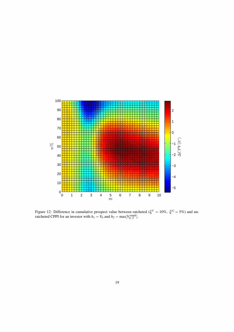
Figures 10 and 11 demonstrated that a ratchet designed to protect 50% of the maximum wealth maynot specifically suit an investor with a w = 50%. In the following two figures: Figure 12 and Figure 13,the difference in CPV between the standard CPPI and a ratcheted ξV = 10%, ξ G = 5% strategy is shownfor w values from 0-100%. Figure 12 clearly shows that the ratcheted CPPI is preferred for a broad areaaround m = 6 and a weighting of 50%. The effect of 200% maximum leverage is shown in Figure 13.Compared to Figure 12, the area where the ratcheted CPPI is preferred is shifted down and to the right.The difference is also significantly smaller. A ξV = 10%, ξ G = 5% ratchet would benefit an investorwith w = 40% more than one with w = 50% when leverage is permitted because the unratcheted strategyattains higher maximums. The ratcheted strategy reduces exposure and growth resulting in it protectingonly 40% rather than 50% of the unratcheted CPPI’s maximum.

When there is no leverage a trough is present for multiplier values between 2 and 3. With a maximumleverage of 200% there is a trough between 3 and 4. In both cases there is a larger negative value whenthere is a higher preference weighting. This feature can be explained as follows. The CPV increasesmost under a CPPI strategy when there is strong growth and therefore a high payoff. However, for highermultiplier values the leverage constraint prevents increased investment in the risky asset resulting in 100%

17

1 2 3 4 5 6 7 8 9 10−40

−30

−20

−10

0

10

CPV(h

∗)

m

No Ratchet ξV =5%, ξG=2.5%

ξV =10%, ξG=5% ξV =15%, ξG=7.5%

ST VrfT

Figure 11: Cumulative prospect value using a reference point of w = 40%, h1 =V0 and h2 = max[V stand0..T ].

Given for various multiplier values and ratcheted and unratcheted CPPI with 200% maximum leverage(l = 200%).

18

0 1 2 3 4 5 6 7 8 9 100

10

20

30

40

50

60

70

80

90

100

m

w%

∆CPV(h

∗ )

−5

−4

−3

−2

−1

0

1

2

Figure 12: Difference in cumulative prospect value between ratcheted (ξV = 10%, ξ G = 5%) and un-ratcheted CPPI for an investor with h1 =V0 and h2 = max[V stand

0..T ].

19

0 1 2 3 4 5 6 7 8 9 100

10

20

30

40

50

60

70

80

90

100

m

w%

∆CPV(h

∗ )

−15

−10

−5

0

Figure 13: Difference in cumulative prospect value between ratcheted (ξV = 10%, ξ G = 5%) and un-ratcheted CPPI for an investor with h1V0 to h2 max[V stand

0..T ] with 200% leverage (l = 200%).

20

(or 200% for the levered approach) investment in S. As demonstrated in Subsection 5.1, increasing theleverage causes a large increase in the CPV so the leverage constraint is a big limiting factor. This affectsboth the standard and ratcheted strategies. However, for the lower multiplier values, where the troughsoccur, the leverage constraint does not have much impact. Instead the ratcheting of the floor is the biggestinhibitor of growth because capital is allocated away from the risky asset to the risk-free asset. The resultis that the standard CPPI outperforms the ratcheted CPPI.

6 ConclusionConstant proportion portfolio insurance is a widely used investment strategy. Dichtl and Drobetz (2010,2011) support the view that investors of CPPI have a preference structure adequately described by cumu-lative prospect theory. However, a conflict occurs with the introduction of a ratcheted floor. Ratchetedfloor products (including time-invariant portfolio protection) are extensions (alternatives) to the CPPI thatare popular with investors. Under CPT however, our results have show that a ratcheted floor is not pre-ferred over the standard CPPI. This is because the ratchet protects increasing levels of wealth while thereference point remains static at the initial wealth value. Since the ratchet limits upside growth in orderto protect greater wealth levels it is not rewarded under the standard fixed reference point cumulativeprospect theory.

In this paper we have proposed an extension to CPT accommodate both the ideas that investors useCPT, but also like ratcheted investments. We have proposed that the investor does not have a fixedreference point, but rather it adapts over time. Specifically, the investor uses a linear combination of theirinitial wealth V0 and the current observed maximum risky price value max[V0..T ]. The evidence in thispaper supports our proposed framework with the investor with an adaptive reference point preferring theratcheted CPPI over the plain model in some cases. More generally our results suggest that the CPTinvestor prefers to have the guarantee minimum payoff match their reference point. This allows the losspart of the value function to be completely ignored producing a higher prospect theory value.

ReferencesArkes, H., Hirshleifer, D., Jiang, D., Lim, S., Jan. 2008. Reference point adaptation: Tests in the domain

of security trading. Organizational Behavior and Human Decision Processes 105 (1), 67–81.

Balder, S., Brandl, M., Mahayni, A., 2009. Effectiveness of CPPI strategies under discrete-time trading.Journal of Economic Dynamics & Control 33 (1), 204–220.

Basak, S., Jul. 2002. A comparative study of portfolio insurance. Journal of Economic Dynamics andControl 26 (7-8), 1217–1241.

Ben Ameur, H., 2010. GARCH Models with CPPI Application. In: Jawadi, F., Barnett, W. A. (Eds.),Nonlinear Modeling of Economic and Financial Time-Series. (International Symposia in EconomicTheory and Econometrics, Volume 20. Emerald Group Publishing Limited, pp. 187–205.

Ben Ameur, H., Prigent, J.-l., 2011. CPPI Method with a Conditional Floor. International Journal ofBusiness 16 (3), 218–229.

Bertrand, P., Prigent, J.-l., 2002. Portfolio Insurance the extreme value approach to the CPPI method.Finance 23 (2), 69–86.

Black, F., Jones, R. C., 1987. Simplifying portfolio insurance. Journal of Portfolio Management 14 (1),48–51.

21

Black, F., Perold, A. F., 1992. Theory of constant proportion portfolio insurance. Journal of EconomicDynamics & Control 16 (3-4), 403–426.

Boulier, J.-F., Kanniganti, A., 1995. Expected Performance and Risks of Various Portfolio InsuranceStrategies. In: 5th AFIR Colloquium. Brussels, Belgium, pp. 1093–1124.

Branger, N., Mahayni, A., Schneider, J. C., Jun. 2010. On the optimal design of insurance contracts withguarantees. Insurance: Mathematics and Economics 46 (3), 485–492.

Chen, J.-S., Chang, C.-L., Hou, J.-L., Lin, Y.-T., 2008. Dynamic proportion portfolio insurance usinggenetic programming with principal component analysis. Expert Systems with Applications 35, 273–278.

Choie, K. S., Seff, E. J., 1989. TIPP: Insurance without complexity: Comment. The Journal of PortfolioManagement 16 (1), 107–108.

Cont, R., Tankov, P., Jul. 2009. Constant Proportion Portfolio Insurance in the Presence of Jumps in AssetPrices. Mathematical Finance 19 (3), 379–401.

Dichtl, H., Drobetz, W., 2010. On the Popularity of the CPPI Strategy: A Behavioral-Finance-BasedExplanation and Design Recommendations. The Journal of Wealth Management 13 (2), 41–54.

Dichtl, H., Drobetz, W., Dec. 2011. Portfolio insurance and prospect theory investors: Popularity andoptimal design of capital protected financial products. Journal of Banking & Finance 35 (7), 1683–1697.

Dierkes, M., Erner, C., Zeisberger, S., May 2010. Investment horizon and the attractiveness of investmentstrategies: A behavioral approach. Journal of Banking & Finance 34 (5), 1032–1046.

Do, B. H., 2002. Relative Performance of Dynamic Portfolio Insurance Strategies: Australian Evidence.Accounting and Finance 42 (3), 279–296.

Do, B. H., Faff, R. W., Jun. 2004. Do Futures-Based Strategies Enhance Dynamic Portfolio Insurance?Journal of Futures Markets 24 (6), 591–608.

Estep, T., Kritzman, M., 1988. TIPP: Insurance without complexity. The Journal of Portfolio Management14 (4), 38–42.

Glosten, L. R., Jagannathan, R., Runkle, D. E., 1993. On the Relation Between the Expected Value andthe Volatility of the Nominal Excess Return on Stocks. Journal of Finance 48 (5), 1779–1801.

Hamidi, B., Jurczenko, E., Maillet, B., 2009. A CAViaR Time-Varying Proportion Portfolio Insurance.Bankers, Markets & Investors September- (102), 4–21.

Jessen, C., 2010. Constant Proportion Portfolio Insurance : Discrete-time Trading and Gap Risk Cov-erage. In: 23rd Australasian Finance and Banking Conference 2010. Copenhagen Business School -Department of Finance, pp. 1–24.

Kahneman, D., Tversky, A., Mar. 1979. Prospect Theory: An Analysis of Decision under Risk. Econo-metrica 47 (2), 263.

Koop, G. J., Johnson, J. G., 2010. The Use of Multiple Reference Points in Risky Decision Making.Journal of Behavioral Decision Making 25 (1), 49–62.

Lattimore, P. K., Baker, J. R., Witte, A. D., 1992. The influence of probability on risky choice: A para-metric examination. Journal of Economic Behavior & Organization 17 (3), 377–400.

22

Lee, H.-I., Hsu, H., Chiang, M.-H., Nov. 2010. Portfolio insurance with a dynamic floor. Journal ofDerivatives & Hedge Funds 16 (3), 219–230.

Lin, C., Huang, W., Zeelenberg, M., Dec. 2006. Multiple reference points in investor regret. Journal ofEconomic Psychology 27 (6), 781–792.

Maringer, D., Ramtohul, T., 2011. GP-based rebalancing triggers for the CPPI. In: Computational Intel-ligence for Financial Engineering and Economics (CIFEr), 2011 IEEE Symposium on. pp. 1–8.

Pain, D., 2008. Recent developments in portfolio insurance. Bank of England Quarterly Bulletin Q1 (Re-search and Analysis), 37–46.

Perold, A. F., Sharpe, W. F., 1988. Dynamic Strategies for Asset Allocation. Financial Analysts Jour-nal (February), 16–27.

Schmidt, U., Starmer, C., Sugden, R., May 2008. Third-generation prospect theory. Journal of Risk andUncertainty 36 (3), 203–223.

Tversky, A., Kahneman, D., 1992. Advances in Prospect Theory: Cumulative Representation of uncer-tainty. Journal of Risk and Uncertainty 5 (4), 297–323.

Vrecko, D., Branger, N., 2009. Why is portfolio insurance attractive to investors?http://ssrn.com/abstract=1519344.

A Time Series Statistics

A.1 Model ParametersA GJR-GARCH(1,1) model with Student-t distributed innovations was fitted to daily log-return data fromthe FTSE 100 index, from 8nd March 1990 to 15th December 2010 inclusively. Parameter estimation andsimulations were undertaken using the MATLAB Garch Toolbox. Simulations were of daily log-returnsfor 5 years (1260 realisations) across 106 paths. Table 1 gives the model parameter values and their errors.Test statistics for the innovations are given in Table 2, confirming the null hypothesis that the innovationsare uncorrelated for 30 lags and are t-distributed with 13.291 degrees of freedom. The process yields anexpected annual return and annual volatility of approximately 8% and 16% respectively.

Table 1: Fitted parameter values, standard errors and t-statistics.Parameter Value Standard Error t-Statistic

K 2.7084e-4 1.1308e-004 2.3952ω 1.1744e-006 2.0216e-7 5.8096α1 0.0111 0.0065 1.7141β1 0.9250 0.0068 135.5325ψ1 0.1047 0.0108 9.6616

DoF 13.2910 1.7828 7.4551

A.2 Summary StatisticsThe summary statistics for the log-returns from the FTSE 100 index from 2nd April 1984 to 15th Decem-ber 2010 inclusively is given in Table 3.

23

Table 2: Ljung-Box and Kolmogorov-Smirnov statistics at 5% confidence interval.Ljung-Box KS(30 lags)

p-value 0.5690 0.7568Critical value 43.7730 0.0186Q-statistic 28.0276 -KS Statistic - 0.0092

Table 3: Summary statistics for FTSE 100 daily log-returns.Quantiles:

Mean 2.4741e-4 1% -0.0311Median 6.0529e-4 5% -0.0168Std. dev. 0.0112 10% -0.0118Skewness -0.3868 25% -0.0054Kurtosis 11.7876 75% 0.0064Min -0.1303 90% 0.0118Max 0.0938 95% 0.0163

99% 0.0286

24