Consistency relations for non- standard models of...

Consistency relations for non-standard models of inflation

Jorge NoreñaPUCV

Based mostly on:

P. Creminelli, J. Noreña, M. Simonović, arXiv: 1203.4595 [hep-th]L. Bordin, P. Creminelli, M. Mirbabayi, J. Noreña, arXiv: 1605.08424 [astro-ph.CO]L. Bordin, P. Creminelli, M. Mirbabayi, J. Noreña, arXiv: 1701.04382 [astro-ph.CO]

Outline

• Introduction, inflation and non-Gaussianity

• Adiabatic modes

• Scalar consistency relation

• Tensor consistency relation

• Solid consistency

k2

k11

1

k3

k1

Non-Gaussianityh⇣(~k1)⇣(~k2)⇣(~k3)i = (2⇡)3�(~k1 + ~k2 + ~k3)B(k1, k2, k3)

Squeezed limit: k1 ⌧ k2, k3

00.5

k2

k11

1

k3

k1



Equilateral configurations: k1 = k2 = k3

00.5

k2

k11

1

k3

k1




Enfolded configurations:

00.5

k1 = 2k2 = 2k3

k2

k11

1

k3

k1





00.5

k1 = 2k2 = 2k3

f loc

NL

= 2.7± 5.8

fequiNL = �42± 75

forth

NL

= �25± 39

PLANCK, 2013

k2

k11

1

k3

k1





00.5

k1 = 2k2 = 2k3

f loc

NL

= 2.7± 5.8

fequiNL = �42± 75

forth

NL

= �25± 39

PLANCK, 2013J. Maldacena, 2003

The information about the non-linearity of the evolution of the perturbations from inflation all the way to the LSS is contained in higher-order correlation functions

h�(q)�(k1)�(k2)i = (2⇡)3�(q+ k1 + k2)B(q, k1, k2)

Setup


We will be interested in the limit

h�(q)�(k1)�(k2)i = (2⇡)3�(q+ k1 + k2)B(q, k1, k2)

h�(q)�(k1) . . . �(kn)iq!0= h�(q)h�(k1) . . . �(kn)i�Li

�L

�S

q ⌧ k1, k2

Setup


We will be interested in the limit

h�(q)�(k1)�(k2)i = (2⇡)3�(q+ k1 + k2)B(q, k1, k2)

h�(q)�(k1) . . . �(kn)iq!0= h�(q)h�(k1) . . . �(kn)i�Li

�L

�S

q ⌧ k1, k2

Setup

Khouri, Hinterbickler, Hui, Joyce, 2012

Khouri, Hinterbickler, Hui, Joyce, 2013

Ghosh, Kundu, Raju, Trivedi, 2014

Goldberger, Hui, Nicolis, 2013

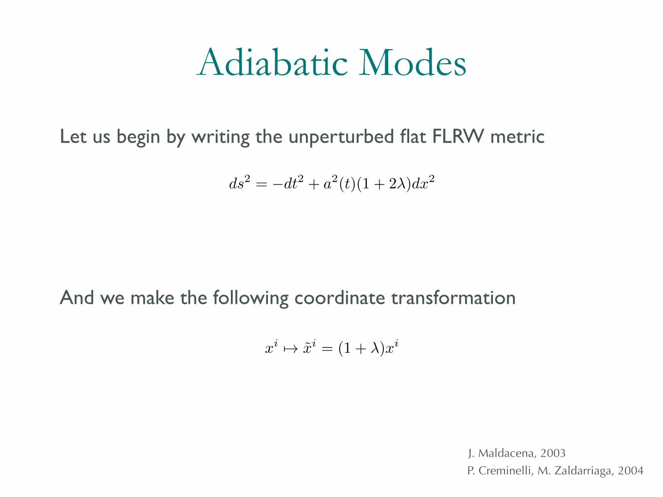
Adiabatic Modes

Let us begin by writing the unperturbed flat FLRW metric

ds

2 = �dt

2 + a

2(t)dx2

P. Creminelli, M. Zaldarriaga, 2004

J. Maldacena, 2003

Adiabatic Modes


And we make the following coordinate transformation

x

i 7! x̃

i = (1 + �)xi

ds

2 = �dt

2 + a

2(t)dx2


J. Maldacena, 2003

Adiabatic Modes



x

i 7! x̃

i = (1 + �)xi

ds

2 = �dt

2 + a

2(t)(1 + 2�)dx2


J. Maldacena, 2003

Adiabatic Modes



⇣ = �

x

i 7! x̃

i = (1 + �)xi

ds

2 = �dt

2 + a

2(t)(1 + 2�)dx2


J. Maldacena, 2003

⇣ = � = const.

Adiabatic Modes

For inflation, out of the horizon



⇣ = �

x

i 7! x̃

i = (1 + �)xi

ds

2 = �dt

2 + a

2(t)(1 + 2�)dx2

I never assumed dS!


J. Maldacena, 2003

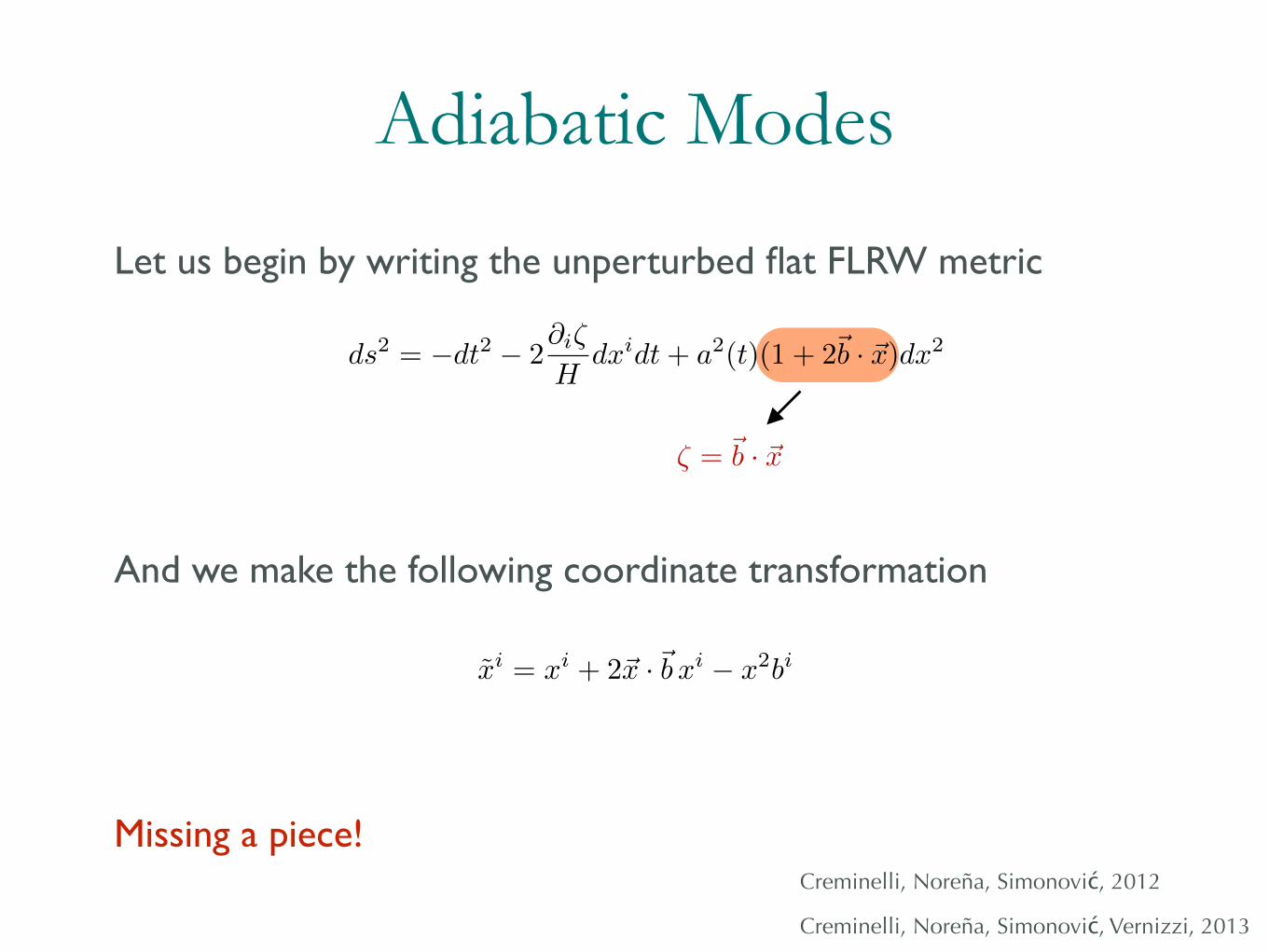
Adiabatic Modes



x̃

i = x

i + 2~x ·~b xi � x

2b

i

⇣ = ~

b · ~x

Missing a piece!

ds

2 = �dt

2 + a

2(t)(1 + 2~b · ~x)dx2

Creminelli, Noreña, Simonović, 2012

Creminelli, Noreña, Simonović, Vernizzi, 2013

Adiabatic Modes



⇣ = ~

b · ~x

ds2 = �dt2 � 2@i⇣

Hdxidt+ a2(t)(1 + 2~b · ~x)dx2

x̃

i = x

i + 2~x ·~b xi � x

2b

i

Missing a piece!Creminelli, Noreña, Simonović, 2012


Adiabatic Modes



⇣ = ~

b · ~x

Valid in FLRW!

ds2 = �dt2 � 2@i⇣

Hdxidt+ a2(t)(1 + 2~b · ~x)dx2

x̃i = xi + 2~x ·~b xi � x2bi �Z

dt1

a2Hbi

Creminelli, Noreña, Simonović, 2012


Squeezed limit informationThe squeezed limit contains model independent information aboutthe physics during inflation

H

B(q, k1, k2)q!0⇠

1

q

Single field


J. Maldacena, 2003

P. Creminelli, G. D’Amico, M. Musso, JN, 2011

The squeezed limit contains model independent information aboutthe physics during inflation

H

B(q, k1, k2)q!0⇠

1

q

1

q3

Single field Multi field

Squeezed limit information


H

B(q, k1, k2)q!0⇠

1

q

1

q↵1 < ↵ < 3

1

q3

Single field Multi field

X. Chen, J. Wang, 2009



H

B(q, k1, k2)q!0⇠

1

q

1

q↵1 < ↵ < 3

1

q31

q↵↵ > 3

?

Single field Multi field Not inflation

Assassi, Baumann, Green, 2012P. Creminelli, JN, M. Simonović, 2012P. Creminelli, G. D’Amico, M. Musso, JN, 2011



H

B(q, k1, k2)q!0⇠

1

q

1

q↵1 < ↵ < 3

1

q31

q↵↵ > 3

?

Single field Multi field Not inflation?

Features

Non-trivialvacua


GravitonsThe ones above are not the only adiabatic modes

Hinterbichler, Hui, Khoury, 2012


Make the following coordinate transformation

Sii = 0x̃ = Sijxj

ds

2 = �dt

2 + a

2(t)dx2





Sii = 0x̃ = Sijxj

ds

2 = �dt

2 + a

2(t)(�ij + 2Sij)dxidx

j





Sii = 0x̃ = Sijxj

ds

2 = �dt

2 + a


j

�ij = 2Sij





Sii = 0x̃ = Sijxj

ds

2 = �dt

2 + a


j

�ij = 2Sij

Implies that the correlation is trivial for a long wavelengthgraviton.

h�⇣⇣i

Tensor CR is very generalThe scalar consistency relation can be broken by additional scalarfields sourcing the curvature perturbation. But scalar fields can’tsource tensors.

J. Maldacena, N. Arkani-Hamed, 2015


What about fields with s > 0 ?




If the background is approximately de Sitter

At late times ⌘ ! 0 �± =3

2±r

9

4� m2

H2t / ⌘�±

h✏2.S~k ✏̃2.S�~ki

0 / e2i + 43��

�ei + 6

(3��)(2��)

(��1)�+ 4

3��

�e�i + e�2i ,




If the background is approximately de Sitter

At late times ⌘ ! 0 �± =3

2±r

9

4� m2

H2t / ⌘�±

h✏2.S~k ✏̃2.S�~ki

0 / e2i + 43��

�ei + 6

(3��)(2��)

(��1)�+ 4

3��

�e�i + e�2i ,

� > 1 Higuchi bound


e.g.

How to break it ?

A. Riotto, A. Kehagias, 2017

We need to break the de Sitter isometries:

1. No breaking of isotropy

2. Breaking isotropy

⇤hµ⌫ = 0+ r↵f(t)r↵hµ⌫

You can arrange it to get h / ⌘0

H. Lee, D. Baumann, G. Pimentel, 2016

Several theories have a preferred spatial frame, e.g. solid inflation,gauge-flation.

A. Maleknejad, M. Sheikh-Jabbari, 2011

S. Endlich, A. Nicolis, J. Wang, 2013

Observations ?Observing the squeezed limit of h�⇣⇣i


1. Look for it directly in the CMB hBTT i

(S/N)

2 ' f�

NL2A

s

r

✓`T,max

`T,min

◆2

log

✓`B,max

`B,min

◆

Meerburg et. al., 2016



2. Local modulation of the matter power spectrum

(S/N)

2 ' f�

NL2A

s

r

✓`T,max

`T,min

◆2

log

✓`B,max

`B,min

◆


P⇣(~k) = P⇣(k)h1 + f�

NL✏sij k̂ik̂j�

s(q)i

(S/N)2 ' 2fs

45⇡f�

NL2rA

s

✓kmax

kmin

◆3

�N

Bartolo et. al., 2014



2. Local modulation of the matter power spectrum

(S/N)

2 ' f�

NL2A

s

r

✓`T,max

`T,min

◆2

log

✓`B,max

`B,min

◆


P⇣(~k) = P⇣(k)h1 + f�

NL✏sij k̂ik̂j�

s(q)i

(S/N)2 ' 2fs

45⇡f�

NL2rA

s

✓kmax

kmin

◆3

�N

3. Matter 4-point function

Bartolo et. al., 2014

(S/N)2 ' ⇡

6075f�

NL4r2A2

s

✓kmax

kmin

◆6

Jeong, Kamionkowski, 2012

Solid inflation: a non-trivial caseSeveral scalar fields with an isotropy-breaking vev h�Ii / x

I

But the background is isotropic if are a vector under SO(3)�I

Perturbations: �I = �̄I + ⇡I

Action written in terms of SO(3) invariants, e.g. @µ�I@µ�I

@µ�I@⌫�I@

µ�J@⌫�J

S. Endlich, A. Nicolis, J. Wang, 2013

Inflation happens if the energy densitydepends very weakly on the volume.

(approximate )�I 7! ��I

Solid inflation breaks isotropy and violates the standard consistencyrelations.

Solid inflation: a non-trivial case



However, it does have an adiabatic mode:

This cancels the perturbations.

�I = �̄I + ⇡Ih�Ii / x

I

x

i 7! x

i � ⇡

i





But it’s not physical! It doesn’t leave the metric untouched.

�I = �̄I + ⇡Ih�Ii / x

I

x

i 7! x

i � ⇡

i





But it’s not physical! It doesn’t leave the metric untouched.

However, the changes in the metric go to zero after an angular average.

This implies a consistency relation for angular-averaged correlationfunctions.

�I = �̄I + ⇡Ih�Ii / x

I

x

i 7! x

i � ⇡

i

Conclusions• Non-Gaussianity allows us to measure the interactions

and non-linearity of the very early universe.

• The effect of a very long wavelength perturbation can be

written as a change of frame, if the evolution of the

Universe is adiabatic.

• Tensor consistency relations hold for a very large class of

models of inflation.

• A non-trivial case study of this logic is solid inflation.

THE END

An “average equivalence principle”

A homogeneus gravitational potential has no physical meaning


� ! 0



A homogeneus gravitational force can be set to zero by going to a freely falling frame

� ! 0



A homogeneus gravitational force can be set to zero by going to a freely falling frame

� ! 0

r� ! 0

~V ! ~V � tr�


Electromagnetic adiabatic modes

Mirbababyi, Simonović, 2016

Electromagnetism also has adiabatic modes:

Aµ 7! Aµ + @µ↵ � 7! ei�Q� A0 = 0

But the gauge is not yet completely fixed @0↵ = 0

These solutions have zero frequency, but they can be continued tofinite-frequency solutions.

The constraint equation is @0@iAi = 0 =) r2↵ = 0

(�@20 +r2)Ai � @i@jA

j = 0The dynamic equation is

One such solution is for example ↵ = ✏ixi

Observations

Dark Energy Task Force stage IV: ⇥�3⇤ � 1/q3/2+�

kmax 0.1 h/Mpc

JN, L. Verde, G. Barenboim, C. Bocsh, 2012

Sefusatti, et. al., 2012

Gank, Komatsu, 2012

Observations

Dark Energy Task Force stage IV: ⇥�3⇤ � 1/q3/2+�

kmax 0.1 h/Mpc

JN, L. Verde, G. Barenboim, C. Bocsh, 2012

Sefusatti, et. al., 2012

Ganc, Komatsu, 2012

Consistency relations for non- standard models of...

Documents

Transcript of Consistency relations for non- standard models of...