Considerations in the Calculation of Vertical Velocity … in the Calculation of Vertical Velocity...
30
Considerations in the Calculation of Vertical Velocity in Three-Dimensional Circulation Models Richard A. Luettich, Jr. University of North Carolina at Chapel Hill Institute of Marine Sciences Morehead City, NC, USA 28557 Julia C. Muccino Department of Civil and Environmental Engineering Arizona State University Tempe, AZ, USA 85287 Michael G. G. Foreman Department of Fisheries and Oceans Institute of Ocean Sciences Sidney, British Columbia, CANADA V8L 4B2 Submitted to: Journal of Atmospheric and Oceanic Technology Date: January 8, 2002
Transcript of Considerations in the Calculation of Vertical Velocity … in the Calculation of Vertical Velocity...
Considerations in the Calculation of Vertical Velocityin Three-Dimensional Circulation Models
Richard A. Luettich, Jr.University of North Carolina at Chapel Hill
Institute of Marine SciencesMorehead City, NC, USA 28557
Julia C. MuccinoDepartment of Civil and Environmental Engineering
Arizona State UniversityTempe, AZ, USA 85287
Michael G. G. ForemanDepartment of Fisheries and Oceans
Institute of Ocean SciencesSidney, British Columbia, CANADA V8L 4B2
Submitted to: Journal of Atmospheric and Oceanic TechnologyDate: January 8, 2002
1/29
1. AbstractThe vertical velocity, , in three-dimensionalcirculationmodelsis typically computed
from the three-dimensionalcontinuity equation assumingthat the depth-varying horizontal
velocityfield wascalculatedearlierin thesolutionsequence.Computing in thiswayappearsto
requirethesolutionof anover-determinedsystemsincethecontinuityequationis first order, yet
mustsatisfytwo boundaryconditions(oneat the freesurfaceandoneat thebottom).At least
threemethodshave beenpreviously proposedto compute : (i) the “traditional” methodthat
solvesthe continuity equationwith the bottomboundaryconditionandignoresthe free surface
boundarycondition,(ii) a “vertical derivative” methodthat solves the vertical derivative of the
continuityequationusingbothboundaryconditionsand(iii) an“adjoint” approachthatminimizes
acostfunctionalcomprisedof residualsin thecontinuityequationandin bothboundaryconditions.
Thelattersolutionis equivalentto the"traditional"solutionplusacorrectionthatincreaseslinearly
over thedepthandis proportionalto themisfit betweenthe"traditional"solutionat thesurfaceand
the surface boundary condition.
In thispaperweshow thatthe"verticalderivative" methodyieldsinaccurateandphysically
inconsistentresultsif it is discretizedas hasbeenpreviously proposed. However, if properly
discretizedthe"verticalderivative" methodis equivalentto the“adjoint” methodif thecostfunc-
tion is weightedto exactly satisfythe boundaryconditions. Furthermore,if the horizontalflow
field satisfiesthe depth-integratedcontinuity equationlocally, oneof the boundaryconditionsis
redundantand obtainedfrom the"traditional" methodshouldmatchthefreesurfaceboundary
condition. In this case,the “traditional,” “adjoint” andproperlydiscretized“vertical derivative”
approachesyield thesameresultsfor . If thehorizontalflow field is not locally massconserving,
themassconservationerroris transferredinto thesolutionfor . Thisis particularlyimportantfor
models that do not guarantee local mass conservation, such as some finite element models.
w
w
w
w
w
w
w
2/29
2. IntroductionThis paperinvestigatesthemeritsof differentapproachesfor calculatingverticalvelocity
fieldsby solvingthethree-dimensionalcontinuityequation,assumingthehorizontalvelocityfields
are known.
In typical three-dimensionalcirculationmodels[e.g.,FUNDY (Lynch and Werner, 1987),
POM (Blumberg and Mellor, 1987),QUODDY (Lynch and Werner, 1991, Lynch and Naimie,
1993),ROMS(Haidvogel and Beckmann, 1999)]theverticalvelocityisdeterminedfromthethree-
dimensional continuity equation:
(1)
where is the horizontalvelocity with components , and
is the vertical velocity. Here arethe horizontalcoordinates, is the vertical
coordinate(positive upward, at themeanwatersurface), is time and is thehorizontal
gradient operator. The kinematic boundary condition on vertical velocity at the bottom is:
at (2a)
where is the mean water depth. The analogous condition at the surface is:
at (2b)
where is thesurfaceelevation.[Note, for future reference, hasbeendefinedasthe
verticalvelocityatthebottomasdeterminedfrom theboundaryconditionand hasbeendefined
astheverticalvelocity at thesurfaceasdeterminedfrom theboundarycondition.]Equations(1),
(2a),(2b)aresolvedfor assumingthatthehorizontalvelocityandsurfaceelevationsareknown
from a previous part of the modelsolution. The primary difficulty of solving theseequationsis
that, together, they constituteanover-determinedsystemof equationsfor themostgeneralcase;
∂w∂z------- ∇ V•–=
V x y z t, , ,( ) u x y z t, , ,( ) v x y z t, , ,( ),( )
w x y z t, , ,( ) x y,( ) z
z 0= t ∇
w V– ∇h• wb= = z h–=
h x y,( )
w∂η∂t------ V ∇η•+ ws= = z η=
η x y t, ,( ) wb
ws
w
3/29
that is, (1) is a firstorder equation that must be solved subject to twoboundary conditions. As will
be shown, in numerical schemes that are locally mass conserving, one of the boundary conditions
becomes redundant and thus the system is not over-determined.
We will consider here two approaches to solving the over-determined system:
1. Solution of the vertical derivative of the continuity equation:
(3)
where indicates vertical velocity computed using the this approach (henceforth,
VDC). This is a second order differential equation and thus both boundary conditions
can be satisfied (Lynch and Naimie, 1993).
2. Solution of the over-determined system in a “best fit” sense by admitting residuals in
the first order continuity equation and both boundary conditions. An optimal solution
is then sought that minimizes those residuals in a weighted least squared sense. Because
this approach involves the adjoint of the continuity equation, we call it the “adjoint”
approach (henceforth, ADJ). It will be described in more detail in Section 3.
A third approach, called the “traditional” approach (TRAD) simply neglects one of the boundary
conditions; this approach will be shown here to be a component of ADJ.
Muccinoet al. (1997) found that VDC and ADJ provide different vertical velocity fields
regardless of resolution in the vertical or horizontal and that ADJ better approximates the analytic
solution in a simple test problem than VDC. The objectives of this paper are to reconcile the numer-
ical differences between VDC and ADJ and to make overall recommendations for the computation
of vertical velocity in three-dimensional circulation models. Results are provided for tidally forced
∂2wvdc
∂z2
----------------∂∂z----- ∇ V•( )–=
wvdc
4/29
circulation in a quarter annular test case and a wind, density and boundary forced circulation off
the southwest coast of Vancouver Island.
3. A summary of the adjoint approach (ADJ)ADJ admits residuals in the continuity equation (1) and the boundary conditions (2a) and
(2b) at each horizontal node:
(4a)
at (4b)
at (4c)
A cost functional, which is formed from the squares of these residuals is defined:
(5)
where , and are constant weights and is the total
water depth and is included in the denominator of the first term to normalize the vertical integral
and also to maintain dimensional consistency. The weights are defined as the inverses of the cova-
riances of the residuals:
, , (6)
where the covariances are defined as:
, , (7)
and indicates expected value. Thus the dimensions of , and are , and
, respectively. We will assume that . Additionally, given that only the relative
f z( ) ∂w∂z------- ∇ V•+=
ib w V ∇h•+= z h–=
is w∂η∂t------ V ∇η•––= z η=
IW f
H-------- f{ }2
dz
h–
η
∫ W b ib{ }2W s is{ }2
+ +=
W f W b W s H x y t, ,( ) h x y,( ) η x y t, ,( )+=
W f1
C f------= W b
1Cb------= W s
1Cs------=
C f f2⟨ ⟩= Cb ib
2⟨ ⟩= Cs is2⟨ ⟩=
⟨ ⟩ W f W b W s T2
T2/L
2
T2/L
2W b W s=
5/29
values of the weights is significant (not the absolute values of the weights themselves) we set
without further loss of generality. Thus, (5) can be written:
(8)
The adjoint solution, , minimizes and can be shown to be:
, (9)
where is the “traditional solution” to the governing equation (1) and the bottom boundary
condition (2a). [For mathematical details leading to (9) see Muccino (1997); for a similar derivation
using “representers,” see Appendix A of Muccino and Bennett (2001)] Thus, the adjoint solution
is a sum of and a correction that is linear in and proportional to the misfit between the tradi-
tional solution evaluated at the surface and the surface boundary condition. In the limit of
(that is, no weight given to the three-dimensional continuity equation in ), the
correction reduces to:
for (10)
In this case, the correction is zero at the bottom and equal to the surface boundary condition misfit
of the traditional solution at the surface. Consequently, the correction causes the adjoint solution
to satisfy both boundary conditions exactly although it may diminish the mass conserving proper-
ties of the solution. In the limit of , (that is, no weight given to the boundary condi-
tions in ) (9) reduces to:
for (11)
In this case, the correction approaches a constant (half the surface boundary condition misfit of the
W b W s 1= =
IW f
H-------- f{ }2
dz
h–
η
∫ ib{ }2is{ }2
+ +=
wadj I
wadj z( ) wtrad z( ) wc z( )+= wc z( ) ws wtrad η( )–( )W f /H
2h z+( )/H+
2W f /H2
1+-----------------------------------------------=
wtrad
wtrad z
W f /H2
0= I
wc z( ) ws wtrad η( )–( )h z+H
-----------= W f /H2
0=
W f /H2 ∞→
I
wc z( )ws wtrad η( )–
2---------------------------------= W f ∞→
6/29
traditional solution) over the depth. This distributes any error evenly between the surface and
bottom boundary conditions, but has no impact on the mass conserving property of the solution.
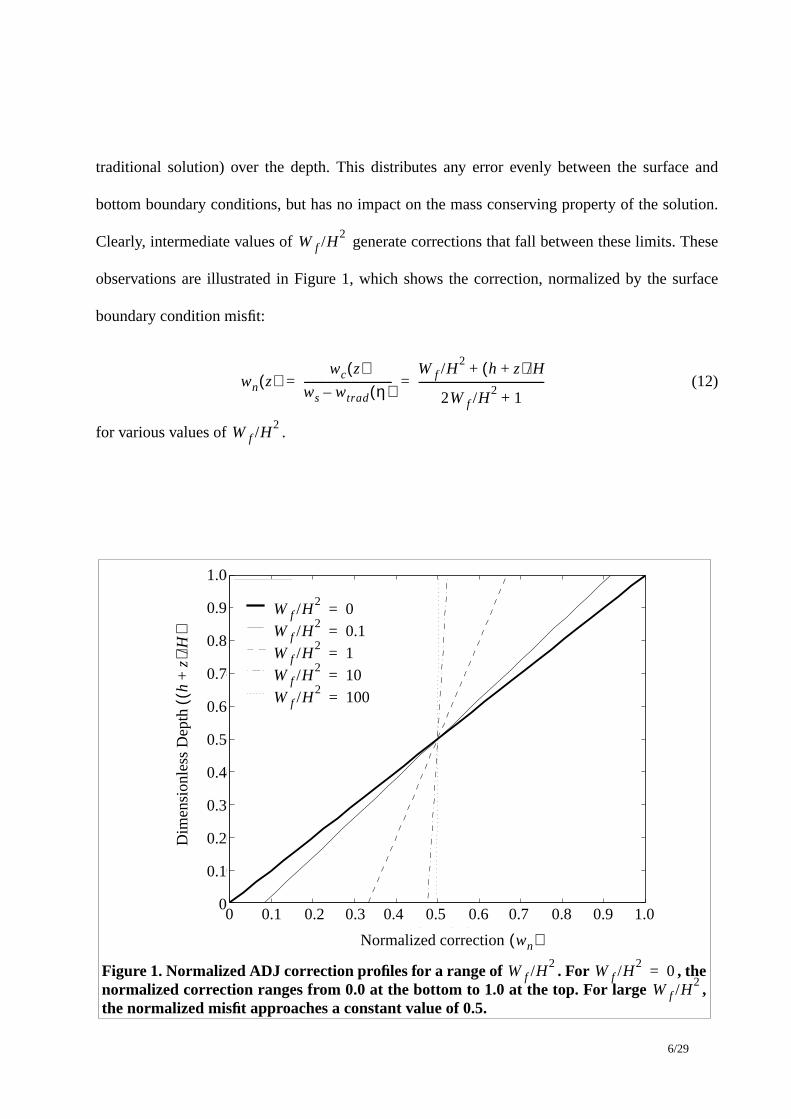
Clearly, intermediate values of generate corrections that fall between these limits. These
observations are illustrated in Figure 1, which shows the correction, normalized by the surface
boundary condition misfit:
(12)
for various values of .
W f /H2
wn z( )wc z( )
ws wtrad η( )–---------------------------------
W f /H2
h z+( )/H+
2W f /H2
1+-----------------------------------------------= =
W f /H2
0 0.1 0.2 0.3 0.4 0.5 0.6 0.7 0.8 0.9 1−1
−0.9
−0.8
−0.7
−0.6
−0.5
−0.4
−0.3
−0.2
−0.1
0Figure 5: Parameters as in Fig. 4: Node 401, Adjoint correction
Amplitude (m/s)
Dim
ensi
onle
ss D
epth
L=0 L=1 L=10 L=100
0.1
0.2
0.3
0.4
0.5
0.6
0.7
0.8
0.9
1.0
0.2 0.4 0.6 0.9
Dim
ensi
onle
ss D
epth
hz
+(
)/H
()
Normalized correction
0.1 0.3 0.5 0.7 0.8
Figure1. Normalized ADJ correctionprofilesfor a rangeof . For , thenormalized correction rangesfr om 0.0 at the bottom to 1.0 at the top. For large ,the normalized misfit approaches a constant value of 0.5.
W f /H2
W f /H2
0=W f /H
2
wn( )1.0
W f /H2
0.1=W f /H
21=
W f /H2
10=W f /H
2100=
W f /H2
0=
00
7/29
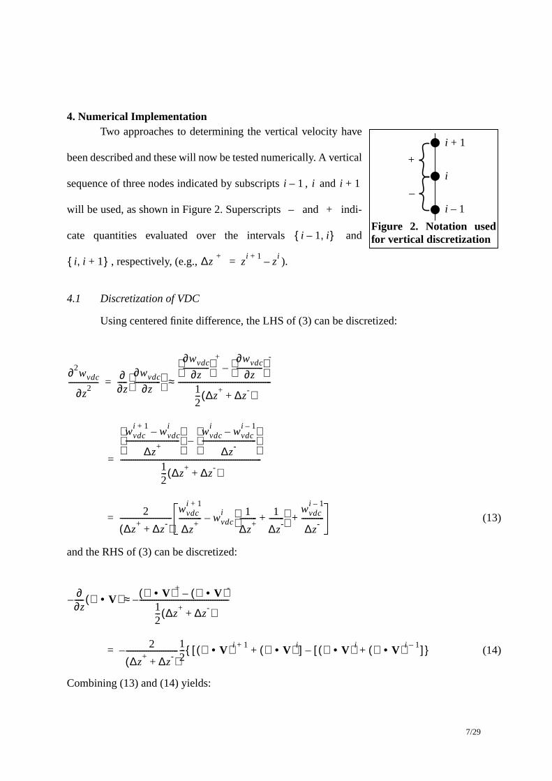
4. Numerical ImplementationTwo approaches to determining the vertical velocity have
been described and these will now be tested numerically. A vertical
sequence of three nodes indicated by subscripts , and
will be used, as shown in Figure 2. Superscripts and indi-
cate quantities evaluated over the intervals and
, respectively, (e.g., ).
4.1 Discretization of VDC
Using centered finite difference, the LHS of (3) can be discretized:
(13)
and the RHS of (3) can be discretized:
(14)
Combining (13) and (14) yields:
i 1+
i
i 1–
Figure 2. Notation usedfor vertical discretization
+
–i 1– i i 1+
– +
i 1– i,{ }
i i 1+,{ } ∆z+
zi 1+
zi
–=
∂2wvdc
∂z2
----------------∂∂z-----
∂wvdc
∂z--------------
∂wvdc
∂z--------------
+ ∂wvdc
∂z--------------
-
–
12--- ∆z
+ ∆z-
+( )--------------------------------------------------≈=
wvdci 1+
wvdci
–
∆z+
----------------------------- wvdc
iwvdc
i 1––
∆z-
-----------------------------
–
12--- ∆z
+ ∆z-
+( )----------------------------------------------------------------------------=
2
∆z+ ∆z
-+( )
----------------------------wvdc
i 1+
∆z+
------------ wvdci 1
∆z+
--------- 1
∆z-
--------+ –
wvdci 1–
∆z-
------------+=
∂∂z-----– ∇ V•( ) ∇ V•( )+ ∇ V•( )-
–12--- ∆z
+ ∆z-
+( )------------------------------------------------–≈
2
∆z+ ∆z
-+( )
----------------------------–12--- ∇ V•( )i 1+ ∇ V•( )i
+[ ] ∇ V•( )i ∇ V•( )i 1–+[ ]–{ }=
8/29
(15)
wherethe ‘+’ and ‘-’ have beenaddedto the two termsinside the curly brackets of (15) as a
reminderthat the first groupin squarebrackets is evaluatedover the interval andthe
second group is evaluated over the interval .
The LHS of (15) is tridiagonalandefficiently solved usinga tridiagonalsolver like the
Thomasalgorithm.The RHS of (15) requiresthe evaluationof the horizontalvelocity on level
coordinatesurfaces.Most three-dimensionalcirculationmodelsusestretchedor terrainfollowing
coordinatesin whichtheverticaldimensionis transformedfrom to , where
and are arbitrary constants (e.g., , ):
(16)
Derivativesin theterrainfollowing coordinatesystemarerelatedto derivativesin thelevel coordi-
nate system using the chain rule:
(17a)
(17b)
where indicateshorizontalderivativesonalevel surfaceand indicateshorizontalderivatives
on a stretched surface. Using (17a) and (17b) to expand terms on the RHS of (15) gives:
wvdci 1+
∆z+
------------ wvdci 1
∆z+
--------- 1
∆z-
--------+ –
wvdci 1–
∆z-
------------+ 12---– ∇ V•( )i 1+ ∇ V•( )i
+[ ]+
∇ V•( )i ∇ V•( )i 1–+[ ]
-–{ }=
i i 1+,{ }
i 1– i,{ }
h– z η< < b σ a< < a
b a 1= b 0=
σ aa b–( ) z η–( )
H----------------------------------+=
∇•V ∇σ•Va b–( )
H---------------- σ b–( )
a b–( )-----------------∇η σ a–( )
a b–( )-----------------∇h+ •
∂V∂σ-------–=
∂∂z-----
a b–( )H
---------------- ∂∂σ------=
∇ ∇σ
9/29
(18a)
(18b)
(18c)
(18d)
Substituting (18a) through (18d) and recognizing that yields:
(19)
In practice, the horizontal derivatives and therefore (19) reduces to:
∇•V( )i 1+[ ]+
∇σ•V( )i 1+ a b–( )H
---------------- σi 1+b–
a b–---------------------
∇η σi 1+a–
a b–---------------------
∇h+ •Vi 1+ Vi
–
∆σ+------------------------
–=
∇•V( )i[ ]+
∇σ•V( )i a b–( )H
---------------- σib–
a b–--------------
∇η σia–
a b–--------------
∇h+ •Vi 1+ Vi
–
∆σ+------------------------
–=
∇•V( )i[ ]-
∇σ•V( )i a b–( )H
---------------- σib–
a b–--------------
∇η σia–
a b–--------------
∇h+ •Vi Vi 1–
–
∆σ-------------------------
–=
∇•V( )i 1–[ ]-
∇σ•V( )i 1– a b–( )H
---------------- σi 1–b–
a b–--------------------
∇η σi 1–a–
a b–--------------------
∇h+ •Vi Vi 1–
–
∆σ-------------------------
–=
∆z H∆σ/ a b–( )=
wvdci 1+
∆σ+------------ wvdc
i 1
∆σ+---------- 1
∆σ----------+
–wvdc
i 1–
∆σ-------------+
12---–
Ha b–( )
---------------- ∇σ•V( )i 1+ ∇σ•V( )i+[ ]
+ Ha b–( )
---------------- ∇σ•V( )i ∇σ•V( )i 1–+[ ]
-–
=
σi 1+b–( )
a b–( )--------------------------∇η σi 1+
a–( )a b–( )
--------------------------∇h+ •Vi 1+ Vi
–
∆σ+------------------------
–
σib–( )
a b–( )------------------∇η σi
a–( )a b–( )
------------------∇h+ •Vi 1+ Vi
–
∆σ+------------------------
Vi Vi 1–
–
∆σ-------------------------
––
σi 1–b–( )
a b–( )-------------------------∇η σi 1–
a–( )a b–( )
-------------------------∇h+ •Vi Vi 1–
–
∆σ-------------------------
+
∇σ•V( )i[ ]+
∇σ•V( )i[ ]-
=
10/29
(20)
where no ambiguity is introduced by dropping the and superscripts on the remaining hori-
zontal velocity gradient terms.
An alternative expression for is obtained from (15) if it is assumed that the horizontal
derivatives . Using the chain rule, (15) reduces to:
(21)
It is clear that (20) and (21) are identical only if . Previous investigators (Lynch
and Naimie, 1993; Muccino et al., 1997) have used an expression for that is equivalent to
wvdci 1+
∆σ+------------ wvdc
i 1
∆σ+---------- 1
∆σ----------+
–wvdc
i 1–
∆σ-------------+
12---–
Ha b–( )
---------------- ∇σ•V( )i 1+ ∇σ•V( )i 1––[ ]
=
σi 1+b–( )
a b–( )--------------------------∇η σi 1+
a–( )a b–( )
--------------------------∇h+ •Vi 1+ Vi
–
∆σ+------------------------
–
σib–( )
a b–( )------------------∇η σi
a–( )a b–( )
------------------∇h+ •Vi 1+ Vi
–
∆σ+------------------------
Vi Vi 1–
–
∆σ-------------------------
––
σi 1–b–( )
a b–( )-------------------------∇η σi 1–
a–( )a b–( )
-------------------------∇h+ •Vi Vi 1–
–
∆σ-------------------------
+
+ -
wvdc
∇•V( )i[ ]+
∇•V( )i[ ]-
=
wvdci 1+
∆σ+------------ wvdc
i 1
∆σ+---------- 1
∆σ----------+
–wvdc
i 1–
∆σ-------------+
12---–
Ha b–( )
---------------- ∇σ•V( )i 1+ ∇σ•V( )i 1––[ ]
=
σi 1+b–( )
a b–( )--------------------------∇η σi 1+
a–( )a b–( )
--------------------------∇h+ •Vi 1+ Vi
–
∆σ+------------------------
–
σi 1–b–( )
a b–( )-------------------------∇η σi 1–
a–( )a b–( )
-------------------------∇h+ •Vi Vi 1–
–
∆σ-------------------------
+
∂V∂σ-------
+ ∂V∂σ-------
-=
wvdc
11/29
(21). However, results from Muccino et al. (1997) show that these values of do not agree with
vertical velocities obtained with ADJ. Below, we demonstrate that (20) does yield values that are
essentially identical to ADJ, while (21) yields significantly inferior estimates of vertical velocity.
4.2 Discretization of ADJ
Recall, the adjoint solution, (9), consists of the sum of the traditional solution (the
solution of the governing equation using the bottom boundary condition and neglecting the surface
boundary condition) plus a correction. Thus, the numerical solution proceeds by first finding
by discretizing (1):
(22)
Using the chain rule, this becomes:
(23)
The calculation is initiated using the bottom boundary condition, and then marched up the water
column; no matrix solver is required. Once is known, is easily computed algebraically
and added to to yield the adjoint solution, .
wvdc
wtrad
wtrad
wtradi
wtradi 1–
–
∆z-
-------------------------------12--- ∇ V•( )i ∇ V•( )i 1–
+[ ]–=
wtradi
wtradi 1–
–
∆σ--------------------------------
12--- H
a b–------------ ∇σ•V( )i ∇σ•V( )i 1–
+[ ]
–=
σib–( )
a b–( )------------------∇η σi
a–( )a b–( )
------------------∇h+ •Vi Vi 1–
–
∆σ-------------------------–
σi 1–b–( )
a b–( )-------------------------∇η σi 1–
a–( )a b–( )
-------------------------∇h+ •Vi Vi 1–
–
∆σ-------------------------–
wtrad wc
wtrad wadj
12/29
4.3 Comparison of VDC and ADJ
Consider VDC first. The second order equation should admit, in addition to the solution of
the associated first order equation, terms that are linear and constant in . For example, suppose
the vertical velocity that satisfies the first order equation (1) is:
(24a)
Consider a different vertical velocity field with addition terms, linear and constant in :
(24b)
where and are constants. The second derivatives of both (24a) and (24b) are:
(25)
Thus, the additional terms in the vertical velocity are transparent in VDC. Furthermore, since the
VDC solution is forced to satisfy both boundary conditions, these terms take on a form such that
satisfies both boundary conditions.
Now consider ADJ with . Equation (10) can be written in the form of (24b),
where:
(26)
and therefore:
, . (27)
Thus, VDC and ADJ with should theoretically yield the same vertical velocity solu-
tion. Indeed, this equivalence is found numerically when (20) is used for the VDC solution
z
w z( ) g z( )=
z
w z( ) g z( ) c1z c2+ +=
c1 c2
∂w2
∂z2
--------- ∂g2
∂z2
--------=
w z( )
W f /H2
0=
g z( ) wtrad z( ) ws wtrad η( )–( ) zH---- ws wtrad η( )–( ) h
H----+ +=
c1
ws wtrad η( )–( )H
--------------------------------------= c2 ws wtrad η( )–( ) hH----
=
W f /H2
0=
13/29
although it does not occur when (21) is used for the VDC solution. This is demonstrated below
using two different test problems.
5. Quarter Annular Harbor Test CaseWe begin numerical tests in a quarter annular harbor with quadratic bathymetry and peri-
odic boundary forcing; the analytic vertical velocity for this problem is given in Muccino et al.
(1997) and thus serves as a useful starting point for comparing the accuracy of these approaches.
That solution is repeated in the Appendix for convenience.
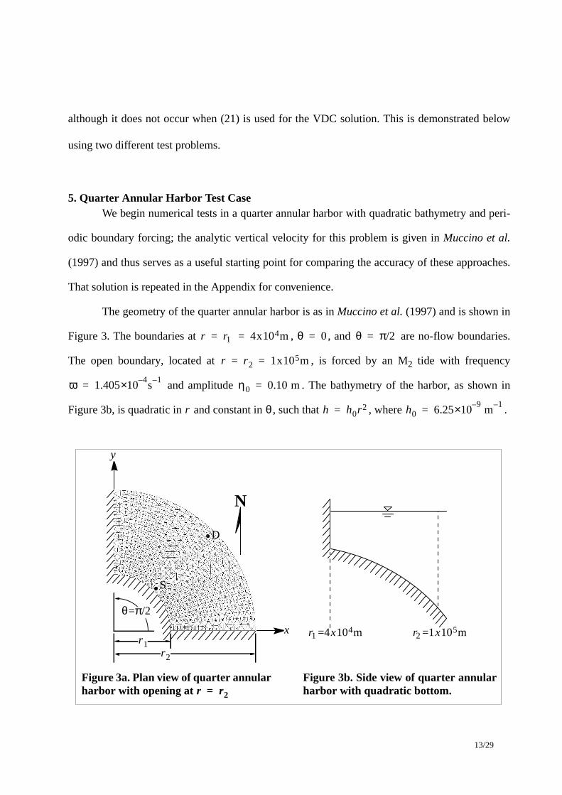
The geometry of the quarter annular harbor is as in Muccino et al. (1997) and is shown in
Figure 3. The boundaries at , , and are no-flow boundaries.
The open boundary, located at , is forced by an M2 tide with frequency
and amplitude . The bathymetry of the harbor, as shown in
Figure 3b, is quadratic in and constant in , such that , where .
r r1 4x10⁴m= = θ 0= θ π/2=
r r2 1x10⁵m= =
ω 1.4054–×10 s
1–= η0 0.10 m=
r θ h h0r2= h0 6.259–×10 m
1–=
r1r2
Figure 3b. Side view of quarter annularharbor with quadratic bottom.
Figure 3a. Plan view of quarter annularharbor with opening at r r2=
θ π/2=
r1 4x10⁴m= r2 1x10⁵m=x
y
N
S
D
14/29
The horizontal velocity is calculated using the analytic solution in Lynch and Officer
(1985); the horizontal velocities are calculated analytically, rather than numerically, so that any
deviations of the numeric vertical velocity solution from the analytic vertical velocity solution
owe entirely to the vertical velocity solution technique, not numerical errors in the horizontal
velocity.
However, evaluation of horizontal velocity derivatives is considered to be a component of
the vertical velocity calculation procedure. Thus (20), (21) and (23) are discretized in the horizon-
tal using Galerkin finite elements with linear basis functions. The solution is evaluated using the
grid shown in Figure 3a. The grid has 825 nodes and 1536 elements in the horizontal and 32
evenly spaced sigma layers in the vertical. Results are presented here for the two representative
nodes shown in the figure: Node S is shallow ( ) and Node D is deep
( ).
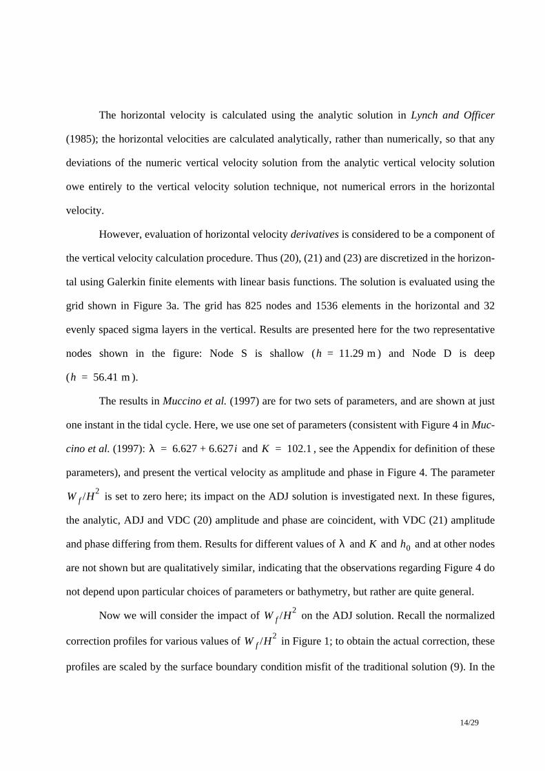
The results in Muccino et al. (1997) are for two sets of parameters, and are shown at just
one instant in the tidal cycle. Here, we use one set of parameters (consistent with Figure 4 in Muc-
cino et al. (1997): and , see the Appendix for definition of these
parameters), and present the vertical velocity as amplitude and phase in Figure 4. The parameter
is set to zero here; its impact on the ADJ solution is investigated next. In these figures,
the analytic, ADJ and VDC (20) amplitude and phase are coincident, with VDC (21) amplitude
and phase differing from them. Results for different values of and and and at other nodes
are not shown but are qualitatively similar, indicating that the observations regarding Figure 4 do
not depend upon particular choices of parameters or bathymetry, but rather are quite general.
Now we will consider the impact of on the ADJ solution. Recall the normalized
correction profiles for various values of in Figure 1; to obtain the actual correction, these
profiles are scaled by the surface boundary condition misfit of the traditional solution (9). In the
h 11.29 m=
h 56.41 m=
λ 6.627 6.627i+= K 102.1=
W f /H2
λ K h0
W f /H2
W f /H2
15/29
quarter annular harbor, the magnitude of this misfit is two or three orders of magnitude smaller than
. Thus, the ADJ correction is insignificant, regardless of the value of , and ADJ
essentially collapses to the traditional approach.
6. Application to the Pacific Coast of Southwest Vancouver Island.The summer circulation off the western continental margin of Vancouver Island is charac-
terized by a moderately intense upwelling of nutrients that supports high biological productivity
0 0.2 0.4 0.6 0.8 1 1.2 1.4 1.6
x 10−5
−1
−0.9
−0.8
−0.7
−0.6
−0.5
−0.4
−0.3
−0.2
−0.1
0
230 235 240 245 250 255 260 265 270 275−1
−0.9
−0.8
−0.7
−0.6
−0.5
−0.4
−0.3
−0.2
−0.1
0
230 235 240 245 250 255 260 265 270 275−1
−0.9
−0.8
−0.7
−0.6
−0.5
−0.4
−0.3
−0.2
−0.1
0
Vertical velocity phase (degrees)235 245 255 265 275
Node D(Phase)
0 0.2 0.4 0.6 0.8 1 1.2 1.4 1.6
x 10−5
−1
−0.9
−0.8
−0.7
−0.6
−0.5
−0.4
−0.3
−0.2
−0.1
0
0 0.2 0.4 0.6 0.8 1.0 1.2 1.4 1.6
Dim
ensi
onle
ss D
epth
zh
+(
)/H
Dim
ensi
onle
ss D
epth
zh
+(
)/H
0
1
0
1
0 0.2 0.4 0.6 0.8 1.0 1.2 1.4 1.6 235 245 255 265 275
Node S(Amplitude)
Node D(Amplitude)
Node S(Phase)
AnalyticADJ, VDCVDC
(20)(21)
Figure 4. Amplitude and phase of vertical velocity in the quarter annular harbor at Node Sand Node D. Note that the analytic, ADJ and VDC (20) solutions are coincident, butdifferent from the VDC (21) solution.
Vertical velocity amplitude (m/s)5–×10
5–×10
wtrad W f /H2
16/29
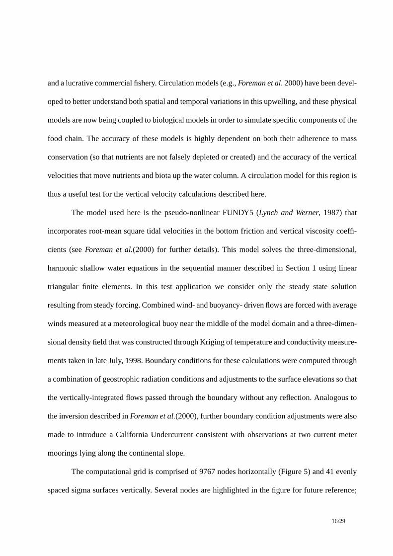
and a lucrative commercial fishery. Circulation models (e.g., Foreman et al. 2000) have been devel-
oped to better understand both spatial and temporal variations in this upwelling, and these physical
models are now being coupled to biological models in order to simulate specific components of the
food chain. The accuracy of these models is highly dependent on both their adherence to mass
conservation (so that nutrients are not falsely depleted or created) and the accuracy of the vertical
velocities that move nutrients and biota up the water column. A circulation model for this region is
thus a useful test for the vertical velocity calculations described here.
The model used here is the pseudo-nonlinear FUNDY5 (Lynch and Werner, 1987) that
incorporates root-mean square tidal velocities in the bottom friction and vertical viscosity coeffi-
cients (see Foreman et al.(2000) for further details). This model solves the three-dimensional,
harmonic shallow water equations in the sequential manner described in Section 1 using linear
triangular finite elements. In this test application we consider only the steady state solution
resulting from steady forcing. Combined wind- and buoyancy- driven flows are forced with average
winds measured at a meteorological buoy near the middle of the model domain and a three-dimen-
sional density field that was constructed through Kriging of temperature and conductivity measure-
ments taken in late July, 1998. Boundary conditions for these calculations were computed through
a combination of geostrophic radiation conditions and adjustments to the surface elevations so that
the vertically-integrated flows passed through the boundary without any reflection. Analogous to
the inversion described in Foreman et al.(2000), further boundary condition adjustments were also
made to introduce a California Undercurrent consistent with observations at two current meter
moorings lying along the continental slope.
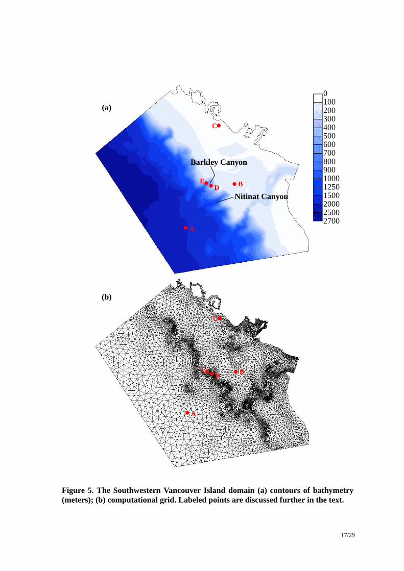
The computational grid is comprised of 9767 nodes horizontally (Figure 5) and 41 evenly
spaced sigma surfaces vertically. Several nodes are highlighted in the figure for future reference;
17/29
Figure 5. The Southwestern Vancouver Island domain (a) contours of bathymetry(meters); (b) computational grid. Labeled points are discussed further in the text.
A
ED
B
C
A
ED B
C
Barkley Canyon
Nitinat Canyon
(a)
(b)
0100200300400500600700800900100012501500200025002700
18/29
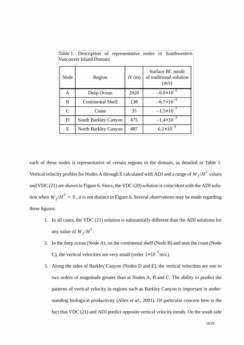
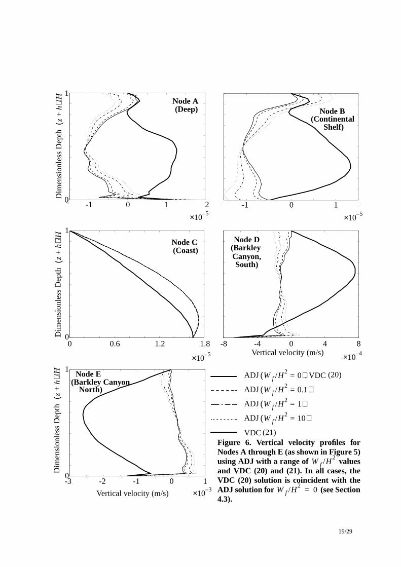
each of these nodes is representative of certain regions in the domain, as detailed in Table 1.
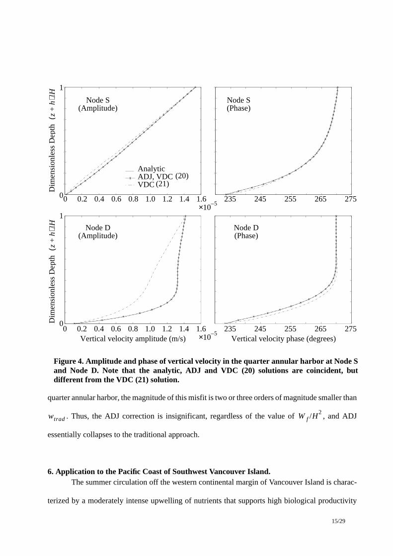
Vertical velocity profiles for Nodes A through E calculated with ADJ and a range of values
and VDC (21) are shown in Figure 6. Since, the VDC (20) solution is coincident with the ADJ solu-
tion when , it is not distinct in Figure 6. Several observations may be made regarding
these figures:
1. In all cases, the VDC (21) solution is substantially different than the ADJ solutions for
any value of .
2. In the deep ocean (Node A), on the continental shelf (Node B) and near the coast (Node
C), the vertical velocities are very small (order ).
3. Along the sides of Barkley Canyon (Nodes D and E), the vertical velocities are one to
two orders of magnitude greater than at Nodes A, B and C. The ability to predict the
patterns of vertical velocity in regions such as Barkley Canyon is important in under-
standing biological productivity (Allen et al., 2001). Of particular concern here is the
fact that VDC (21) and ADJ predict opposite vertical velocity trends. On the south side
W f /H2
W f /H2
0=
Table 1. Description of representative nodes in SouthwesternVancouver Island Domain
Node Region (m)Surface BC misfit
of traditional solution(m/s)
A Deep Ocean 2020
B Continental Shelf 138
C Coast 35
D South Barkley Canyon 475
E North Barkley Canyon 487
H
6.05–×10–
6.75–×10–
1.57–×10–
1.43–×10–
6.23–×10
W f /H2
15–×10 m/s
19/29
−3 −2.5 −2 −1.5 −1 −0.5 0 0.5 1
x 10−3
−1
−0.9
−0.8
−0.7
−0.6
−0.5
−0.4
−0.3
−0.2
−0.1
0Figure 10e: Barkley Canyon, North (Node 6946), R=6201e−6
−8 −6 −4 −2 0 2 4 6 8
x 10−4
−1
−0.9
−0.8
−0.7
−0.6
−0.5
−0.4
−0.3
−0.2
−0.1
0Figure 10d: Barkley Canyon, South (Node 6114), R=−2842e−6
0 0.2 0.4 0.6 0.8 1 1.2 1.4 1.6 1.8
x 10−5
−1
−0.9
−0.8
−0.7
−0.6
−0.5
−0.4
−0.3
−0.2
−0.1
0Figure 10c: Coast (Node 7794), R=−0.15e−6
−1.5 −1 −0.5 0 0.5 1 1.5
x 10−5
−1
−0.9
−0.8
−0.7
−0.6
−0.5
−0.4
−0.3
−0.2
−0.1
0Figure 10b: Shelf (Node 4049, R=−68e−6)
−1.5 −1 −0.5 0 0.5 1 1.5 2
x 10−5
−1
−0.9
−0.8
−0.7
−0.6
−0.5
−0.4
−0.3
−0.2
−0.1
0Figure 10a: Deep (Node 4257, R=478e−6)
Figure 6. Vertical velocity profiles forNodes A through E (as shown in Figure 5)using ADJ with a range of valuesand VDC (20) and (21). In all cases, theVDC (20) solution is coincident with theADJ solution for (see Section4.3).
W f /H2
W f /H2
0=
Node ANode B
Node C Node D
(Deep)(Continental
(Coast) (Barkley
South)
Node E(Barkley Canyon
North)
0 21-15–×10
-1 0 15–×10
5–×10
0 0.6 1.2 1.8 -4 4 84–×10
-3 -1 03–×10
ADJ W f /H2
0=( ) VDC,
ADJ W f /H2
0.1=( )
ADJ W f /H2
1=( )
ADJ W f /H2
10=( )
VDC
Vertical velocity (m/s)
Vertical velocity (m/s)
Dim
ensi
onle
ss D
epth
zh
+(
)/H
Dim
ensi
onle
ss D
epth
zh
+(
)/H
Dim
ensi
onle
ss D
epth
zh
+(
)/H 1
0
1
0
1
0
(21)
(20)
-2 1
Shelf)
Canyon,
-8 0
20/29
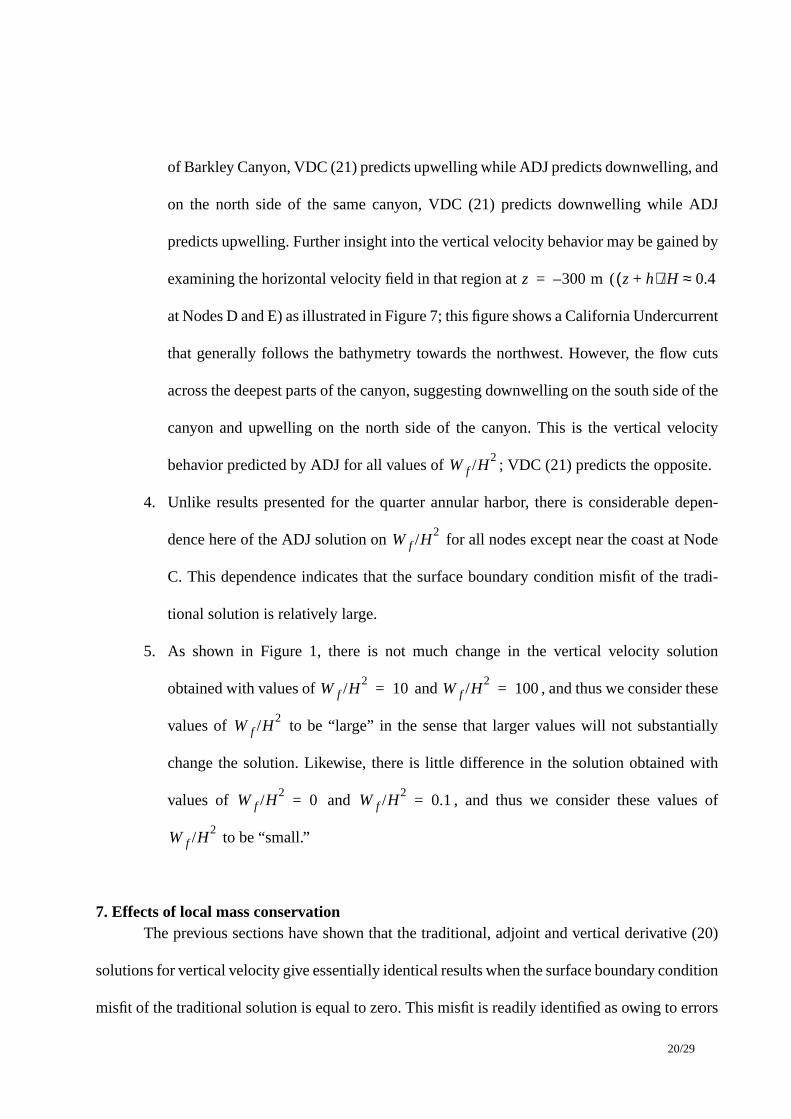
of Barkley Canyon, VDC (21) predicts upwelling while ADJ predicts downwelling, and
on the north side of the same canyon, VDC (21) predicts downwelling while ADJ
predicts upwelling. Further insight into the vertical velocity behavior may be gained by
examining the horizontal velocity field in that region at (
at Nodes D and E) as illustrated in Figure 7; this figure shows a California Undercurrent
that generally follows the bathymetry towards the northwest. However, the flow cuts
across the deepest parts of the canyon, suggesting downwelling on the south side of the
canyon and upwelling on the north side of the canyon. This is the vertical velocity
behavior predicted by ADJ for all values of ; VDC (21) predicts the opposite.
4. Unlike results presented for the quarter annular harbor, there is considerable depen-
dence here of the ADJ solution on for all nodes except near the coast at Node
C. This dependence indicates that the surface boundary condition misfit of the tradi-
tional solution is relatively large.
5. As shown in Figure 1, there is not much change in the vertical velocity solution
obtained with values of and , and thus we consider these
values of to be “large” in the sense that larger values will not substantially
change the solution. Likewise, there is little difference in the solution obtained with
values of and , and thus we consider these values of
to be “small.”
7. Effects of local mass conservationThe previous sections have shown that the traditional, adjoint and vertical derivative (20)
solutions for vertical velocity give essentially identical results when the surface boundary condition
misfit of the traditional solution is equal to zero. This misfit is readily identified as owing to errors
z 300 m–= z h+( )/H 0.4≈
W f /H2
W f /H2
W f /H2
10= W f /H2
100=
W f /H2
W f /H2
0= W f /H2
0.1=
W f /H2
21/29
in the horizontal solution. Integrating (1) from the bottom upward and applying the bottom
boundary condition (2a) yields:
(28)
Applying Liebnitz’s Rule to the integral in (28) yields:
(29)
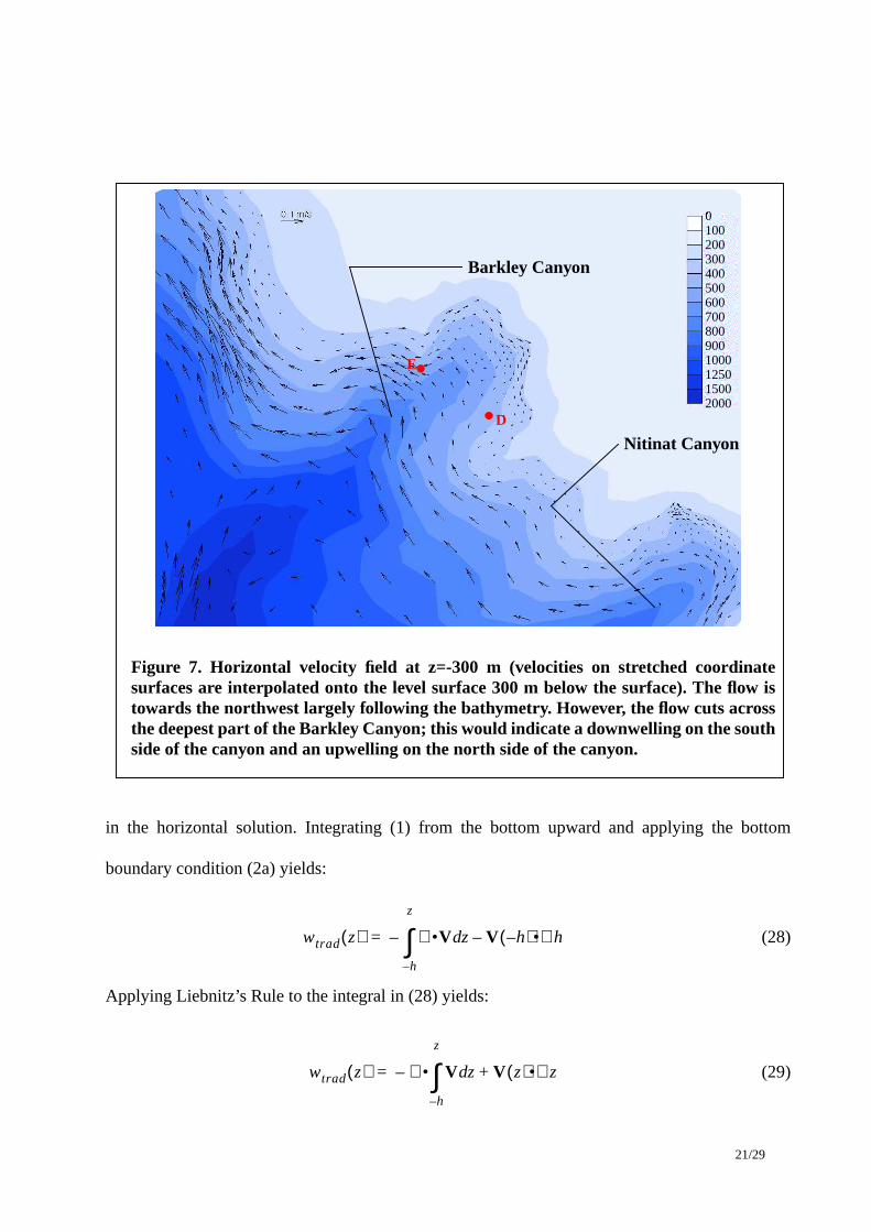
Figure 7. Horizontal velocity field at z=-300 m (velocities on stretched coordinatesurfacesare interpolated onto the level surface 300 m below the surface).The flow istowards the northwest largely following the bathymetry. However, the flow cuts acrossthe deepestpart of the Barkley Canyon; this would indicate a downwelling on the southside of the canyon and an upwelling on the north side of the canyon.
Barkley Canyon
Nitinat Canyon
E
D
01002003004005006007008009001000125015002000
wtrad z( ) ∇•V zd
h–
z
∫– V h–( )•∇h–=
wtrad z( ) ∇• V zd
h–
z
∫– V z( )•∇z+=
22/29
In the interior of the water column, and the vertical velocity is simply the horizontal diver-
gence of the horizontal velocity field integrated up from the bottom. At the free surface, (29)
becomes:
(30)
Using the surface boundary condition (2b) to replace the final term in (30) and rearranging gives:
(31)
The RHS of (31) is the vertically-integrated continuity equation. Consequently, (31) shows that the
misfit between the traditional solution evaluated at the surface and the surface boundary condition
is nonzero anywhere in the domain that the horizontal velocity field does not conserve mass in the
vertically-integrated sense. Since numerical models solve discrete rather than continuous
governing equations, discretization of the vertically-integrated continuity equation in (31) must
match that used to evaluate (1), (2a) and (2b).Thus, local mass conservation, on the same numerical
stencil used to determine , is required if the misfit on the LHS of (31) is to be zero. If mass is not
locally conserved, error is introduced into the computed vertical velocity field as it is integrated up
the water column.
The quarter annular test problem presented in Section 5 uses horizontal velocities obtained
from the analytical solution and thus these velocities satisfy the vertically-integrated continuity
equation exactly; the surface misfit is insignificant and VDC (20) and ADJ with any value of the
parameter give essentially identical results throughout the domain.
∇z 0=
wtrad η( ) ∇• V zd
h–
η
∫– V η( )•∇η+=
ws wtrad η( )– ∂η∂t------ ∇• V zd
h–
η
∫+=
w
W f /H2
23/29
While finite difference models using Arikawa C grids conserve mass on each computa-
tional cell, Galerkin finite element models are guaranteed to conserve mass only globally (Lynch,
1985; Lynch and Holboke, 1997) and therefore allow for nonzero local residuals in the vertically-
integrated continuity equation. Figure 8 illustrates the surface misfits for the Vancouver Island test
problem; by (31), this plot also represents local vertically-integrated continuity residuals. Consid-
erable surface misfits are observed; areas having large misfits (and thus poor vertically-integrated
mass conservation) typically correspond to areas of steep bathymetric gradients. Plots of surface
misfits or vertically-integrated mass error such as this are easy to construct and provide a useful
diagnostic tool for identifying areas where local mass conservation is relatively poor, and therefore
where significant errors are likely to exist in the vertical velocity solution.
As outlined earlier, most oceanic circulation models follow a sequential solution procedure
in which the vertical velocity solution occurs separate from and with minimal feed back to the hori-
zontal velocity solution. Since mass conservation error in the horizontal solution is the cause of the
vertical velocity solution error identified above, it seems inadvisable to sacrifice the boundary
condition information in favor of stricter adherence to the three-dimensional continuity equation
when determining the vertical velocity. Consequently, we suggest a small value of the ADJ
weighting parameter ( ) as preferable to a high value ( ).
8. ConclusionsThe results presented in this paper help reconcile past uncertainty in the vertical velocity
solution in three-dimensional circulation models. Specifically, we have found the following.
1. Most three-dimensional circulation models use a sequential solution procedure to solve
for the free surface elevation and velocity fields. That is, the vertically-integrated conti-
W f /H2
W f /H2
0.1< W f /H2
10>

24/29
nuity and the three-dimensional momentum equations are solved first for the free
surface elevation and the horizontal velocity fields; then the three-dimensional conti-
nuity equation is solved for the vertical velocity field. Solving the three-dimensional
continuity equation (a first order differential equation in the vertical coordinate) for the
vertical velocity would appear to be problematic given the need to satisfy boundary
conditions at both the bottom and at the free surface. However, the “traditional”
Figure 8. Misfit between the traditional solution at the surface and the surfaceboundary condition for the Vancouver Island domain. Filled, colored contoursrepresent misfits, and contour lines represent bathymetry (with the same contourintervals as Figure 5). Residuals are largest in regions of sharply varying bathymetry.
-25.0-5.0-1.0-0.20.21.05.0
25.03–×10
25/29
(TRAD) vertical velocity solution, obtained by integrating the three-dimensional conti-
nuity equation upward using the bottom boundary condition, will match the surface
boundary condition if the elevation and horizontal velocity fields exactly satisfy the
vertically-integrated continuity equation. In this case, the surface boundary condition is
redundant. If the elevation and horizontal velocity fields are not locally mass
conserving, the misfit between the TRAD solution and the surface boundary condition
is equal to the local error in the vertically-integrated continuity equation.
2. The VDC approach proposed by Lynch and Naimie (1993), in which the vertical
velocity is computed from the vertical derivative of the three-dimensional continuity
equation, is equivalent to an optimal, adjoint solution (ADJ) of the three-dimensional
continuity equation (Muccino et al., 1997) in which the boundary conditions are
preserved in lieu of stricter adherence to the continuity equation. VDC requires the
solution of a tri-diagonal matrix problem over the vertical while ADJ requires no matrix
solution. Thus ADJ is more computationally efficient than VDC.
3. Depending upon the numerical discretization applied to VDC, results are obtained that
are less accurate than the other vertical velocity solutions in the quarter annular harbor
test case and that appear to be physically inconsistent in the Vancouver Island test case.
We recommend that if VDC is used, the discretization presented in (20) be used rather
than the discretization presented in (21).
4. The ADJ solution is the solution that minimizes the cost functional (5) which penalizes
misfits to the three-dimensional continuity equation and the misfits of the bottom and
surface boundary conditions. The ADJ solution can be shown to be the sum of the
TRAD solution and a linear correction. In the limit of satisfying both the bottom and
26/29
free surface boundary conditions ( ) the correction is zero at the bottom and
equal to the misfit of the TRAD solution and the free surface boundary condition at the
surface. In the limit of maximizing adherence to the three-dimensional continuity equa-
tion, , the correction is a constant over the entire water column and equal
to one half of the misfit of the TRAD solution and the free surface boundary condition.
5. If there is no misfit between the TRAD solution and the free surface boundary condi-
tion, TRAD, ADJ and VDC (20) give identical solutions for the vertical velocity.
6. Results from models that do not enforce strict local mass conservation, such as finite
element models, will be susceptible to the vertical velocity errors described herein. We
recommend plotting maps of the error in the vertically-integrated continuity equation
as a diagnostic tool for determining areas in the domain that may be subject to signifi-
cant vertical velocity errors. The first choice for improving the computed vertical
velocity is to reduce errors in vertically-integrated mass conservation, either by
improved grid resolution or by smoothing the bathymetry (Oliveira et al., 2000). Mass
conservation may also be improved in Generalized Wave Continuity Equation based
finite element models by increasing the primitive continuity equation weighting param-
eter (known as or ), (Kolar et al., 1992, 1994). If local mass conservation cannot
be achieved, we suggest use of ADJ with the weighting coefficient set to preferentially
favor the surface and bottom boundary conditions ( ).
9. AcknowledgementsThe authors would like to thank Chris Naimie for independently confirming that the results
presented here are consistent with FUNDY5. The authors also thank Rick Thomson, Susan Allen,
Dave Mackas and the crew of the CCGS John P. Tully for collecting the salinity, temperature, and
W f /H2
0=
W f /H2
10>
τ0 G
W f /H2
0.1<
27/29
velocity data that were used in this study. These observations were taken during a GLOBEC
Canada cruise that was co-sponsored by the Natural Sciences and Engineering Research Council
of Canada and the Department of Fisheries and Oceans. R. Luettich would like to acknowledge
partial funding for this work by the Office of Naval Research award N00014-97-C-6010 and J.
Muccino would like to acknowledge partial funding for this work by the National Science Foun-
dation under OCE-9520956.
10. Appendix: Analytic solution quarter annular harborConsider a quarter annular harbor with no-flow boundaries at , , and
and an open boundary at . The open boundary is subject to periodic forcing
. The bathymetry of the harbor is quadratic in and constant in , such that
. The eddy viscosity, , and bottom friction, , vary such that:
and , (32)
are constant. The analytic solution for surface elevation and horizontal velocity (Lynch andOfficer,
1985) are:
(33)
(34)
where: ,
,
r r1= θ 0=
θ π/2= r r 2=
η Re η0eiωt{ }= r θ
h h0r 2= N k
KkhN------= λ iωh2
N------------=
η r t,( ) Re Ars1 Br
s2+( ) iωt( )exp
=
v r σ t, ,( ) Re v0 r( ) 1 δ λσ( )cosh–( )eiωt{ }=
Aη0s2r 1
s2
s2r 2
s1r 1
s2 s1r 1
s1r 2
s2–------------------------------------------= B
η– 0s1r 1
s1
s2r 2
s1r 1
s2 s1r 1
s1r 2
s2–------------------------------------------=
s1 1– 1 β2–+= s2 1– 1 β2––=
β2 ω2 iωτ–( )/ gh0( )=
28/29
is the gravitational constant and . The vertical velocity is (Muccino et al., 1997):
(35)
where:
,
11. References
Allen, S. E., C. Vindeirinho, R. E. Thomson, M. G. G. Foreman and D. L. Mackas, 2001: Physicaland biological processes over a submarine canyon during an upwelling event. Canadian Journalof Fisheries and Aquatic Sciences, 59(4), 671-684.
Blumberg, A. F. and G. L. Mellor, 1987: A description of a three-dimensional coastal ocean circu-lation model. In: C.N.K. Mooers, [ed], Three-dimensional Coastal Ocean Models, Coastal andEstuarine Sciences 4, AGU Press, Washington, DC, 1-16.
Foreman, M. G. G., R. E. Thomson, and C. L. Smith, 2000: Seasonal current simulations for thewestern continental margin of Vancouver Island. J. Geophys. Res., 105(C8), 19,665-19,698.
Haidvogel, D.B. and A. Beckmann. 1999: Three-dimensional ocean models. Chapter 4 in Numer-ical Ocean Circulation Modeling, Imperial College Press, London, England, 121-162.
Kolar, R. L., W. G. Gray, J. J. Westerink and R. A. Luettich, Jr., 1994: Shallow water modeling inspherical coordinates: Equation formulation, numerical implementation and application. J.Hydraul. Res., 32(1), 3-24.
τ Nh2----- λ2 λtanh
λ λ2
K----- 1–
λtanh+
---------------------------------------------=
v0 r( ) giωr--------– s1 Ar
s1 s2Brs2+( )=
g i 1–=
w r σ t, ,( ) Re 2γ α1δ σ λσ( )cosh λ( )cosh+( ) λσ( )sinh λ( )sinh+λ
------------------------------------------------–
=
γ α2 σ 1 δ λσ( ) λ( )sinh+sinh( )λ
--------------------------------------------------------–+ 2γ α1 1 δ λ( )cosh–[ ]+ + e
iωt
σ z/h=
γgh0
iω-------- iωt( )exp=
α1 As1rs1 Bs2rs2+= α2 As12rs1 Bs2
2rs2+=
δ 1
λ( )cosh 1λK---- λ( )tanh+
-----------------------------------------------------------=
29/29
Kolar, R. L., W. G. Gray and J. J. Westerink, 1992: An analysis of the mass conserving propertiesof the generalized wave continuity equation. Computational Methods in Water Resources IX, 2,T. Russell et al., [eds], Computational Mechanics Publications, Southampton, UK, pp. 537-544.
Lynch, D.R. and M.J. Holboke, 1997: Normal flow boundary conditions in 3D circulation models.Int. J. Numer. Meth. Fluids, 25, 1185-1205.
Lynch, D. R. and C. E. Naimie, 1993: The M2 tide and its residual on the outer banks of the Gulfof Maine. J. Phys. Oceanogr., 23, pp. 2222-2253.
Lynch, D. R. and F. E. Werner, 1991: Three-dimensional hydrodynamics on finite elements. Part I:Nonlinear time-stepping model. Int. J. Numer. Meth. Fluids, 12, 507-533.
Lynch, D. R. and F. E. Werner, 1987: Three-dimensional hydrodynamics on finite elements. PartII: Linearized harmonic model. Int. J. Numer. Meth. Fluids, 7, 871-909.
Lynch, D. R. and C. B. Officer, 1985: Analytic test cases for three-dimensional hydrodynamicmodels. Int. J. Numer. Meth. Fluids, 5, 529-543.
Lynch, D. R., 1985: Mass balance in shallow water simulations. Communications in AppliedNumerical Methods, 1, 153-159.
Muccino, J.C. and A. F. Bennett, 2001: Generalized inversion of the Korteweg-de Vries Equation.submitted to Dyn. Atmos. Oceans.
Muccino, J. C., W. G. Gray and M. G. G. Foreman, 1997: Calculation of vertical velocity in three-dimensional, shallow water equation, finite element models. Int. J. Numer. Meth. Fluids, 25,779-802.
Oliveira, A., A. B. Fortunato and A. M. Baptista, 2000: Mass balance in Eulerian-Lagrangian trans-port simulations in estuaries. J. Hydraul. Eng., 126, 605-614.