Residual income valuation: Are inflation adjustments necessary?

John O'Hanlon* and Ken Peasnell**

Management SchoolLancaster UniversityLancaster LA1 4YX

UK

July 17, 2003

* John O'Hanlon: email - J.O'hanlon@lancaster.ac.uk; telephone – (44) 1524 593631** Ken Peasnell: email - K.Peasnell@lancaster.ac.uk; telephone – (44) 1524 593977

Residual income valuation: Are inflation adjustments necessary?

Abstract

This paper explores the question of whether the residual income valuation relationship (RIVR)

should be written in inflation-adjusted terms. This question is of particular interest in the light of

Ritter and Warr's (2002) claim that the standard nominal historical cost RIVR undervalues firms

because it fails to deal with inflation. We present three inflation-adjusted formulations of RIVR,

each of which is based on an income measure from the inflation accounting literature, and one of

which is a general case of Ritter and Warr's formulation. We show that none of these

formulations is any more or less correct than the standard formulation of RIVR, and find no

support for the view that it is necessary to write RIVR in inflation-adjusted terms. Finally we

argue that, in a setting in which accounting numbers and forecasts thereof are normally presented

in nominal historical cost terms, the inflation adjustment of RIVR is likely to bring unnecessary

complication to the valuation process, with increased scope for error.

Keywords: Equity valuation, residual income, inflation

JEL classification: M4

Residual income valuation: Are inflation adjustments necessary?

This paper explores the question of whether the residual income-based valuation relationship

(RIVR) should be written in terms of inflation-adjusted residual incomes rather than in terms of

nominal residual incomes. Until recently, the RIVR literature has been silent on the question of

whether and how residual income forecasts should be adjusted to reflect expected inflation. The

standard practice has been to work with nominal forecasts of historical cost residual income,

discounted at the nominal cost of capital. However, a recent study by Ritter and Warr (2002)

(RW) claims that this practice, as exemplified in the empirical work of Lee, Myers and

Swaminathan (1999), can lead to under-valuation of firms. RW claim that for residual income

models to produce accurate measures of true economic value 'they should use real required

returns, adjust depreciation for the distorting effects of inflation, and make adjustments for

leverage-induced capital gains' (RW, pp. 59-60). Bradley and Jarrell (2003) express a similar

concern that accounting-based valuation models, including RIVR, fail to deal properly with the

effect of inflation. In order to remedy the claimed shortcomings of the nominal historical cost-

based RIVR, RW propose a corrected inflation-adjusted formulation. RW report that this gives

value estimates that differ markedly from those given by the nominal historical cost-based RIVR.

Given the central role of RIVR in the theory and practice of accounting-based valuation, the

possibility that RIVR fails to deal properly with the effects of inflation merits detailed analysis.

In this paper, we carry out such an analysis.

In our analysis, we present three formulations of RIVR, each of which is based on an

inflation-adjusted income measure that has appeared in prior literature. The first formulation is

based on current cost residual income. The second is based on real current cost residual income,

being current cost residual income less a purchasing-power capital maintenance charge. These

two residual income measures derive from income measures familiar from both the seminal work

of Edwards and Bell (1961) and the now-defunct Statement of Financial Accounting Standards

No. 33: Financial Reporting and Changing Prices (Financial Accounting Standards Board,

1979). The third formulation is based on real current cost residual income expressed in real terms

as at the valuation date. This is a development of the residual income measures used in the first

two inflation-adjusted formulations of RIVR, and forms the basis of the RW model. In presenting

the three inflation-adjusted formulations of RIVR, we demonstrate that each is equivalent to the

standard nominal historical cost-based RIVR and that, therefore, none of the three is any more

correct or any less correct than the standard formulation of RIVR. Second, we demonstrate that,

subject to a minor error, the RW model is a special case of the third of our inflation-adjusted

formulations of RIVR, and is likewise no more or less correct than the standard nominal

historical cost-based RIVR. We conclude that there is no logical basis for the view that RIVR

needs to be written in terms of inflation-adjusted residual incomes rather than nominal historical

cost-based residual incomes. In the light of this we argue that, in a setting in which accounting

numbers and forecasts thereof are normally presented in nominal historical cost terms,

complexity and potential for error are likely to be introduced into the valuation process by

working with an inflation-adjusted formulation of RIVR.

The paper is organized as follows. Section 1 outlines the basis for residual income-based

valuation in general, and outlines the criticisms levelled by RW at the nominal historical cost-

based formulation of RIVR. Section 2 presents three inflation-adjusted formulations of RIVR, as

outlined above, and shows that all are theoretically equivalent to the standard nominal historical

2

cost-based formulation of RIVR. Section 3 shows that the RW model is a special case of one of

the inflation-adjusted formulations of RIVR presented in Section 2. Section 4 illustrates the

complexity and potential for error that can be introduced into the valuation process by recasting

nominal historical cost accounting inputs in inflation-adjusted terms. Conclusions are presented

in Section 5.

1. The residual income-based valuation relationship (RIVR)

This section outlines the basis for residual income-based valuation in general, and outlines the

criticisms levelled by RW at the nominal historical cost-based formulation of RIVR.

RIVR has three foundations. The first of these is the present value relationship (PVR)

which is the cornerstone of the theory of asset valuation:

V t=∑s=1

∞

( E t [C t+s ]

∏k=1

s

(1+Re , t+k )), (PVR)

where V denotes the intrinsic value of equity, C denotes dividends net of new equity

contributions, Re ,t +k denotes the one-period nominal cost of equity applicable to the equity

capital as at time t+k-1, and Et [ .] denotes expectations at time t. Here and throughout our

exposition, all transactions are assumed to occur at the end of the relevant period. A second

foundation of RIVR is the assumption that forecasts of dividends, accounting income and book

value comply with the clean surplus relationship (CSR). A general statement of CSR is as

follows:

Bt+s=Bt+ s−1−Ct +s+Y t +s , (CSR)

3

where B denotes the book value of equity and Y denotes accounting income. The third foundation

is the definition of residual income, denoted RI, as income less a capital charge comprising the

product of the cost of equity and the beginning-of-period book value of equity:

RI t +s=Y t+s−Re , t+s Bt+s−1 . (RI)

Provided that Et [ B t+s ] /∏

k=1

s

(1+Re , t+k )→0 as s→∞ ,1 the combination of PVR, CSR and RI

yields the well-known RIVR:2

V t=Bt +∑s=1

∞

( Et [ RI t+ s ]

∏k=1

s

(1+Re , t+k )). (RIVR)

As long as forecast accounting numbers conform to CSR, the estimate of equity value given by

RIVR is equal to the estimate, V t , given by PVR. It is important to note that the theoretical

equivalence between RIVR and PVR does not rely upon the valuation convention used in

arriving at the forecasts of accounting incomes and book values.

We now present the nominal historical cost-based formulation of RIVR that is

conventionally used in the valuation literature, and outline RW's criticism of this formulation.

We represent the historical cost balance sheet of the firm as comprising real (non-monetary)

depreciable assets measured at historical cost net of depreciation, net debt, and equity measured

on a historical cost basis.3 These three items are denoted Ah

, D and Bh

, respectively, where the

superscript h indicates that the accounting number in question is measured on a historical cost

basis. To avoid unnecessary complication, we assume throughout that debt is measured on the

4

same basis under both historical cost and current cost accounting.4 The historical cost book value

of shareholders' equity at time t+s is the excess (or shortfall) of assets over debt:

Bt+sh =A t+s

h −Dt+s . (1)

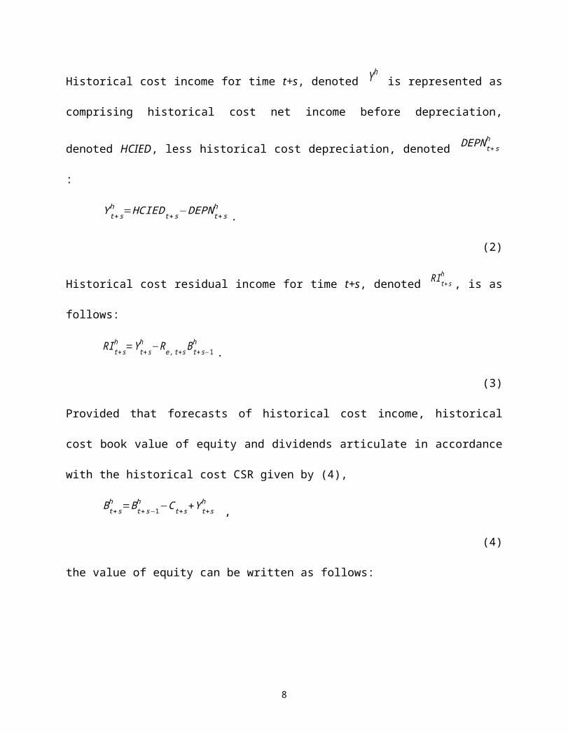
Historical cost income for time t+s, denoted Yh

is represented as comprising historical cost net

income before depreciation, denoted HCIED, less historical cost depreciation, denoted DEPN t +sh

:

Y t+ sh =HCIED t+s−DEPN t +s

h. (2)

Historical cost residual income for time t+s, denoted RI t +sh

, is as follows:

RI t +sh =Y t+s

h −Re , t+s Bt+s−1h

. (3)

Provided that forecasts of historical cost income, historical cost book value of equity and

dividends articulate in accordance with the historical cost CSR given by (4),

Bt+sh =Bt+ s−1

h −Ct +s+Y t +sh

, (4)

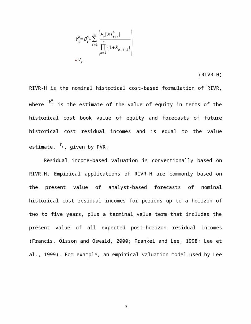
the value of equity can be written as follows:

V th=Bt

h+∑s=1

∞

(E t [ RI t+sh ]

∏k=1

s

(1+Re , t+k ) )¿V t . (RIVR-H)

RIVR-H is the nominal historical cost-based formulation of RIVR, where V th

is the estimate of

the value of equity in terms of the historical cost book value of equity and forecasts of future

historical cost residual incomes and is equal to the value estimate, V t , given by PVR.

5

Residual income-based valuation is conventionally based on RIVR-H. Empirical

applications of RIVR-H are commonly based on the present value of analyst-based forecasts of

nominal historical cost residual incomes for periods up to a horizon of two to five years, plus a

terminal value term that includes the present value of all expected post-horizon residual incomes

(Francis, Olsson and Oswald, 2000; Frankel and Lee, 1998; Lee et al., 1999). For example, an

empirical valuation model used by Lee et al. (1999) and referred to by RW (p. 36) in motivating

their analysis, is as follows:

V th=Bt

h+Et [ RI t +1

h ](1+Re )

+Et [ RI t+ 2

h ]

(1+Re )2 +

E t [ RI t+3h ]

(1+Re)2 Re , (5)

where Re is the (assumed constant) nominal cost of equity. Here, the terminal value term

comprises the nominal historical cost residual income forecast for time t+3 capitalized as a

constant perpetuity.

RW argue (pp. 36-38) that valuation models of the form of (5) have four shortcomings.

First, the post-horizon residual incomes are capitalized as a flat perpetuity, which RW argue

could be related to the erroneous application of a nominal discount rate to real flows. Second,

such models fail to recognize a gain to equity-holders resulting from erosion in the purchasing

power of monetary liabilities due to inflation ('debt capital gain'). Third, the use of the nominal

required rate of return to calculate the residual income capital charge means that, in inflationary

times, residual incomes are underestimated. Fourth, the depreciation expense embedded within

residual income takes no account of increases in the current cost of depreciable assets. RW claim

that the overall effect of these shortcomings will be to cause RIVR to undervalue firms. RW also

present what they claim to be a corrected inflation-adjusted formulation of RIVR, which gives

6

value estimates that differ markedly from those given by the standard formulation of RIVR.

Bradley and Jarrell (2003) express concerns that are related to those of RW, and argue that the

use of earnings or residual incomes in valuation models without inflation adjustment will result

in under-valuation of firms.

RIVR has a central role in the theory and practice of accounting-based valuation. The

claim that the standard nominal historical cost-based formulation of the relationship is deficient

with regard to its treatment of inflation, and that this results in the under-valuation of firms, is a

serious one. In the next section, we present a number of inflation-adjusted formulations of RIVR,

and examine the claimed superiority of these formulations over the nominal historical cost-based

formulation.

2. Residual income valuation using nominal and inflation-adjusted numbers

In this section, we formulate versions of RIVR based on three inflation-adjusted residual income

measures: (i) current cost residual income, (ii) real current cost residual income, being current

cost residual income less a purchasing-power capital maintenance charge, and (iii) real current

cost residual income expressed in real terms as at the valuation date. Current cost residual

income and real current cost residual income are derived from income measures which appear in

the seminal work of Edwards and Bell (1961), and which were required to be disclosed under the

now-defunct Statement of Financial Accounting Standards No. 33. The third measure, real

current cost residual income as restated to real terms at the valuation date, is embedded within

RW's inflation-adjusted formulation of RIVR. The three inflation-adjusted formulations of RIVR

are presented in subsections 2.1, 2.2 and 2.3, respectively. For each inflation-adjusted

7

formulation, we show analytically that the inflation adjustment has no effect on the residual

income-based value estimate.

2.1 Residual income and RIVR on a current cost basis

The first inflation adjustment that we consider involves restating income and residual income to a

current cost basis. We follow the tradition in the literature of assuming that current cost will

normally be defined as the cost of replacing the firm's assets.5 Nothing fundamental is involved

in changing from historical cost to current cost. The current cost book value of shareholders'

equity at time t+s is as follows:

Bt+sc =A t+s

c −Dt+s , (6)

where At +sc

is the cost at time t+s of replacing the non-monetary assets, based on the prices of

those assets, and Bt+sc

is the book value of equity at time t+s measured on a current cost basis.

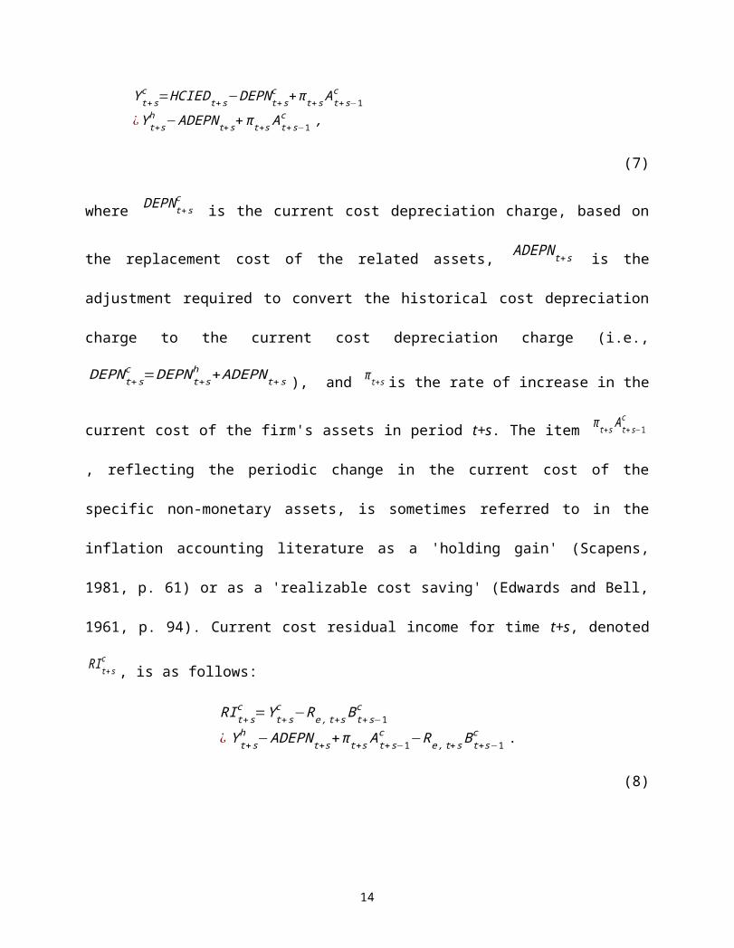
Current cost income for time t+s, denoted Y t+ sc

, is as follows:

Y t+ sc =HCIED t+s−DEPN t +s

c +π t+s A t+s−1c

¿Y t+ sh −ADEPN t+ s+π t+s A t+s−1

c , (7)

where DEPN t +sc

is the current cost depreciation charge, based on the replacement cost of the

related assets, ADEPN t+s is the adjustment required to convert the historical cost depreciation

charge to the current cost depreciation charge (i.e., DEPN t +sc =DEPN t+s

h + ADEPN t+ s ), and

π t+s is the rate of increase in the current cost of the firm's assets in period t+s. The item

π t+s A t+s−1c

, reflecting the periodic change in the current cost of the specific non-monetary assets,

8

is sometimes referred to in the inflation accounting literature as a 'holding gain' (Scapens, 1981,

p. 61) or as a 'realizable cost saving' (Edwards and Bell, 1961, p. 94). Current cost residual

income for time t+s, denoted RI t +sc

, is as follows:

RI t +sc =Y t+s

c −Re , t+s Bt+s−1c

¿ Y t +sh −ADEPN t+ s+π t+s A t+s−1

c −Re , t+s Bt+ s−1c . (8)

Provided that forecasts of current cost income, current cost book value of equity and forecasts of

dividends articulate in accordance with the current cost CSR given by (9),

Bt+sc =Bt+ s−1

c −Ct +s+Y t +sc

, (9)

the value of equity can be written as follows:

V tc=B t

c+∑s=1

∞

(Et [RI t+sc ]

∏k=1

s

(1+Re , t+k ) )¿V t=V t

h . (RIVR-C)

RIVR-C is the current cost-based formulation of RIVR, where, V tc

is the value estimate in terms

of the current cost book value of equity and forecasts of future current cost residual incomes. V tc

is equal to the value estimates, V t and V th

, given by PVR and RIVR-H, respectively. Properly

applied, RIVR-H and RIVR-C must yield the same value estimate, since the accounting in each

conforms to CSR.

2.2 Real current cost residual income

9

The second inflation adjustment that we consider involves the subtraction from current cost

income of a capital maintenance adjustment, to give real current cost income. This income

measure is described in Edwards and Bell (1961), and was required to be disclosed under

Statement of Financial Accounting Standards No. 33. The subtraction from this income measure

of a real capital charge gives real current cost residual income. Real current cost income,

denoted Yc , real

, is calculated by deducting from current cost income the amount by which

opening equity needs to increase over the period in order for its beginning-of-period purchasing

power to be maintained. This capital maintenance adjustment is calculated by reference to the

rate of change in the general price level.6 Real current cost income can be represented as

follows:

Y t+ sc , real=Y t+ s

h −ADEPN t+ s+π t+s A t+s−1c − pt+ s B t+s−1

c , (10)

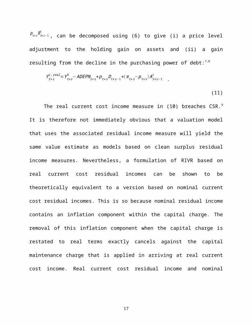
where pt+ s is the periodic rate of change in the general price level for period t+s. The capital

maintenance adjustment in (10), pt+ s B t+s−1c

, can be decomposed using (6) to give (i) a price level

adjustment to the holding gain on assets and (ii) a gain resulting from the decline in the

purchasing power of debt:7,8

Y t+ sc , real=Y t+ s

h −ADEPN t+ s+ pt+s D t+s−1+( π t+s−pt +s ) At +s−1c

. (11)

The real current cost income measure in (10) breaches CSR.9 It is therefore not

immediately obvious that a valuation model that uses the associated residual income measure

will yield the same value estimate as models based on clean surplus residual income measures.

Nevertheless, a formulation of RIVR based on real current cost residual incomes can be shown to

be theoretically equivalent to a version based on nominal current cost residual incomes. This is

10

so because nominal residual income contains an inflation component within the capital charge.

The removal of this inflation component when the capital charge is restated to real terms exactly

cancels against the capital maintenance charge that is applied in arriving at real current cost

income. Real current cost residual income and nominal current cost residual income are therefore

identical, and so are the theoretical value estimates based on the two residual income measures.

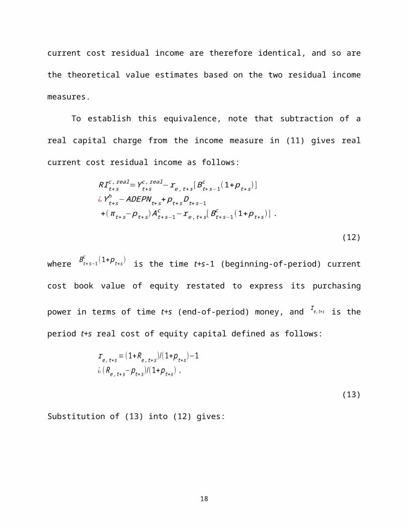
To establish this equivalence, note that subtraction of a real capital charge from the

income measure in (11) gives real current cost residual income as follows:

RI t +sc , real=Y t +s

c , real−r e , t+s [ Bt+ s−1c (1+ pt+ s) ]

¿Y t+ sh −ADEPN t+ s+ pt+s D t+s−1

+( π t+ s−pt +s ) A t+s−1c −re ,t +s [ Bt+s−1

c (1+ pt+s ) ] . (12)

where Bt+s−1c (1+ pt+s ) is the time t+s-1 (beginning-of-period) current cost book value of equity

restated to express its purchasing power in terms of time t+s (end-of-period) money, and re ,t +s is

the period t+s real cost of equity capital defined as follows:

re ,t +s = (1+Re , t+s )/(1+ pt +s )−1¿ (Re , t+s−pt +s )/(1+ p t+s ) . (13)

Substitution of (13) into (12) gives:

RI t+sc , real=Y t+s

h −ADEPN t +s+ pt +s Dt+s−1

+(π t +s−p t+s ) A t+s−1c −( Re , t+ s−p t+s )Bt +s−1

c . (14)

Since Bt+s−1c = A t+s−1

c −Dt +s−1 , the inflation adjustment to the residual income capital charge,

pt+ s B t+s−1c

, cancels exactly against the net of (i) the inflation adjustment to the holding gains on

11

real assets, pt+ s A t+s−1c

, and (ii) the gain from erosion of the purchasing power of debt capital

pt+ s Dt+s−1 . Expression (14) therefore collapses to

RI t +sc , real=Y t +s

h −ADEPN t +s+π t+ s A t+s−1c −Re , t+s Bt+ s−1

c. (15)

Since the right-hand side of (15) contains exactly the same elements as the right-hand side of (8),

it follows that

RI t +sc , real=RI t+s

c . (16)

In other words, real current cost residual income is equal to nominal current cost residual

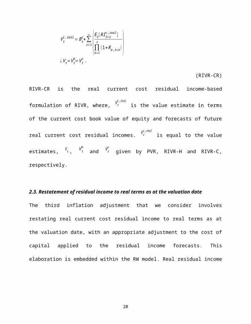
income. From (16) and RIVR-C, the value of equity can be written as follows:

V tc , real = Bt

c+∑s=1

∞

(E t [RI t+sc , real ]

∏k=1

s

(1+Re , t+k ) )¿V t=V t

h=V tc . (RIVR-CR)

RIVR-CR is the real current cost residual income-based formulation of RIVR, where, V tc , real

is

the value estimate in terms of the current cost book value of equity and forecasts of future real

current cost residual incomes. V tc , real

is equal to the value estimates, V t , V th

and V tc

given by

PVR, RIVR-H and RIVR-C, respectively.

2.3. Restatement of residual income to real terms as at the valuation date

The third inflation adjustment that we consider involves restating real current cost residual

income to real terms as at the valuation date, with an appropriate adjustment to the cost of capital

applied to the residual income forecasts. This elaboration is embedded within the RW model.

12

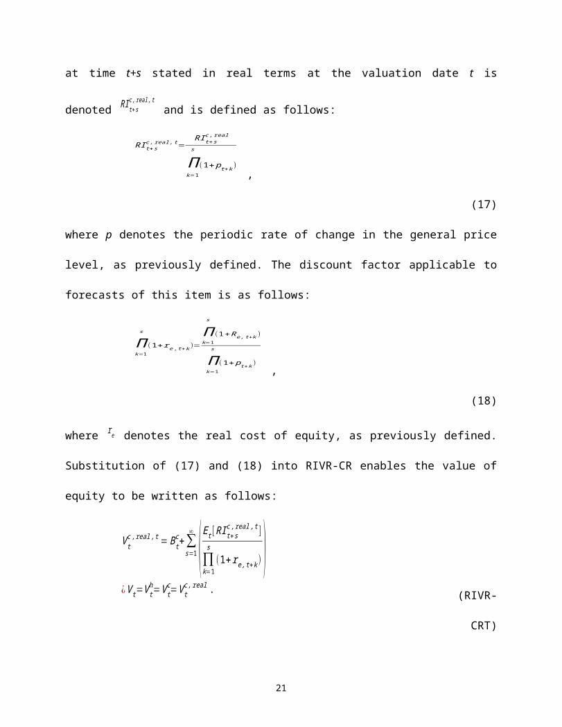
Real residual income at time t+s stated in real terms at the valuation date t is denoted RI t +sc , real , t

and is defined as follows:

RIt +sc , real , t=

RI t+sc , real

Πk=1

s

(1+ p t+k ) , (17)

where p denotes the periodic rate of change in the general price level, as previously defined. The

discount factor applicable to forecasts of this item is as follows:

Πk=1

s

(1+re ,t +k )=

Πk=1

s

(1+Re , t+k )

Πk=1

s

(1+ pt+k ) , (18)

where re denotes the real cost of equity, as previously defined. Substitution of (17) and (18) into

RIVR-CR enables the value of equity to be written as follows:

V tc , real , t = Bt

c+∑s=1

∞

(E t[ RI t +sc , real , t ]

∏k=1

s

(1+re , t+k ) )¿V t=V t

h=V tc=V t

c , real . (RIVR-CRT)

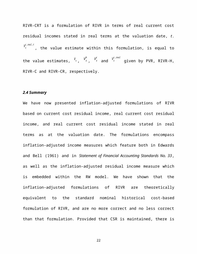
RIVR-CRT is a formulation of RIVR in terms of real current cost residual incomes stated in real

terms at the valuation date, t. V tc , real , t

, the value estimate within this formulation, is equal to the

value estimates, V t , V th

, V tc

and V tc , real

given by PVR, RIVR-H, RIVR-C and RIVR-CR,

respectively.

2.4 Summary

13

We have now presented inflation-adjusted formulations of RIVR based on current cost residual

income, real current cost residual income, and real current cost residual income stated in real

terms as at the valuation date. The formulations encompass inflation-adjusted income measures

which feature both in Edwards and Bell (1961) and in Statement of Financial Accounting

Standards No. 33, as well as the inflation-adjusted residual income measure which is embedded

within the RW model. We have shown that the inflation-adjusted formulations of RIVR are

theoretically equivalent to the standard nominal historical cost-based formulation of RIVR, and

are no more correct and no less correct than that formulation. Provided that CSR is maintained,

there is no theoretical difference between the value estimate obtained from the use of nominal

historical cost residual incomes and that obtained from the use of current cost residual incomes.

Because of the compensating effects of the capital maintenance charge and the inflation

adjustment to the residual income capital charge, the restatement of current cost residual incomes

to real terms should have no effect either. Also, deflation of the real current cost residual incomes

to real terms as at the valuation date, together with use of a real cost of equity rather than a

nominal cost of equity, should have no effect. If the underlying forecasts have been prepared on a

consistent and comparable basis, they should all lead to the same estimates of intrinsic value.

Any differences that could arise must therefore be due to forecasting inconsistencies. After

consideration of the RW model in Section 3, we present in Section 4 a numerical example which

illustrates the equivalences that have been demonstrated in this section, and which illustrates

forecasting inconsistencies that could cause differences between RIVR-H value estimates and

those from inflation-adjusted formulations of RIVR.

14

3. The Ritter-Warr (RW) model

In this section we demonstrate that, with the exception of an insignificant difference that appears

to result from an error in the derivation of the RW model, the RW model is simply a special case

of RIVR-CRT. Expansion of the residual income-related term in RIVR-CRT, by substitution of

(12) and (17) gives

V tc , real , t = Bt

c

+∑s=1

∞ (Et [Y t+ sh

Πk=1

s

(1+ pt+k )

−ADEPN t +s

Πk=1

s

(1+ p t+k )

+pt+s D t+s−1

Πk=1

s

(1+ pt+k )

+(π t +s−p t+s ) A t+s−1

c

Πk=1

s

(1+ pt +k )

−re , t+ s Bt +s−1

c

Πk=1

s−1

(1+ p t+k ) ]∏k=1

s

(1+re ,t +k)) .

(19)

The RW model contains a number of simplifying assumptions. First, the current cost depreciation

adjustment is expected to remain constant in real terms10:

ADEPN t+s=ADEPN t Πk=1

s

(1+ pt+k ) ∀ s . (20)

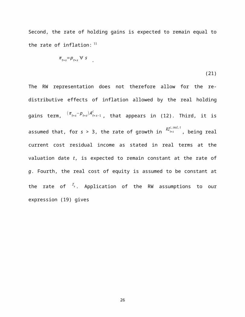
Second, the rate of holding gains is expected to remain equal to the rate of inflation: 11

π t+s=pt +s ∀ s . (21)

The RW representation does not therefore allow for the re-distributive effects of inflation

allowed by the real holding gains term, ( π t+s−pt+ s) At +s−1c

, that appears in (12). Third, it is

assumed that, for s > 3, the rate of growth in RI t +sc , real , t

, being real current cost residual income as

stated in real terms at the valuation date t, is expected to remain constant at the rate of g. Fourth,

15

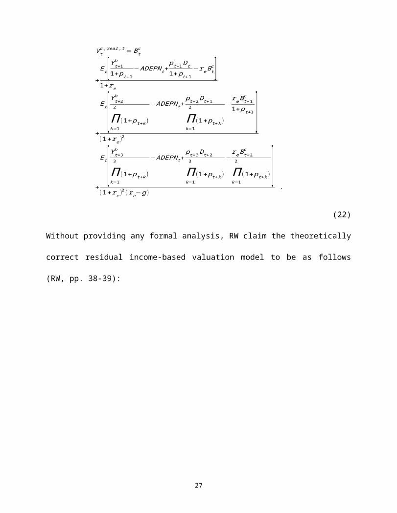
the real cost of equity is assumed to be constant at the rate of re . Application of the RW

assumptions to our expression (19) gives

V tc , real , t = Bt

c

+

E t[Y t +1h

1+ pt+1−ADEPN t+

p t+1 Dt

1+ p t+1−re B t

c]1+r e

+

E t[Y t +2h

Πk=1

2

(1+ pt+k )

−ADEPN t+pt +2 Dt +1

Πk=1

2

(1+ pt +k)

−re Bt+1

c

1+ pt+1 ](1+re)

2

+

E t[Y t +3h

Πk=1

3

(1+ pt+k )

−ADEPN t+pt +3 D t+2

Πk=1

3

(1+ pt +k)

−re Bt+2

c

Πk=1

2

(1+ pt+k ) ](1+re)

2 (re−g ).

(22)

Without providing any formal analysis, RW claim the theoretically correct residual income-based

valuation model to be as follows (RW, pp. 38-39):

V tc , real , t = Bt

c

+

E t[Y t +1h

1+ pt+1−ADEPN t+ p t+1 Dt−re Bt

c]1+r e

+

E t[Y t +2h

Πk=1

2

(1+ pt+k )

−ADEPN t+pt +2 Dt +1

(1+ p t+1)−

re Bt+1c

1+ pt+1 ](1+re)

2

+

E t[Y t +3h

Πk=1

3

(1+ pt+k )

−ADEPN t+pt +3 D t+2

Πk=1

2

(1+ pt +k)

−re Bt+2

c

Πk=1

2

(1+ pt+k ) ](1+re)

2 (re−g ).

(23)

16

Expression (23) differs from (22) only in that the terms reflecting the inflation-related gain on

debt are greater by pt+12 Dt /(1+ pt +1 ) ,

pt+22 Dt +1 /Π

k=1

2

(1+ p t+k ) and pt+3

2 Dt +2/ Πk=1

3

(1+p t+k ),

respectively. This discrepancy appears to be due to an error in the RW model, which wrongly

implies that the debt-related component of the capital maintenance charge in (11) and (19) is

pt+ s Dt+s−1 (1+ p t+s ) rather than pt+ s Dt+s−1 , an overstatement of pt+ s2 Dt+s−1 . To illustrate the

nature of this error, suppose a firm owes $1,000 throughout a year when inflation is 5%. The

amount required to maintain the purchasing power of the amount owing to the creditor is $50 (=

0.05 * $1,000), but RW measure the related adjustment to the real current cost income in (11) as

$52.5 (= 0.05 * $1000 * 1.05), an overstatement of $2.5 (=0.052 * $1000). The impact of this

additional squared inflation-rate term is likely to be empirically unimportant in most cases.

We have shown that the RW model is essentially a special case of the formulation of

RIVR in terms of real current cost residual income stated in real terms at the valuation date. We

have previously shown that this formulation is theoretically equivalent to the standard historical

cost residual income-based valuation model as given by RIVR-H. The RW model is therefore no

more correct and, subject to an insignificant error, no less correct than the standard historical cost

residual income-based valuation model. We may therefore conclude that we find no basis for

RW's claims that the standard historical cost residual income-based valuation model must be

adjusted to deal with inflation and that the RW inflation-adjusted residual income valuation

model is theoretically more correct than the historical cost-based version. If the underlying

forecasts have been prepared on a consistent and comparable basis, they should all lead to the

17

same estimates of intrinsic value. Any differences that could arise in empirical applications must

therefore be due to forecasting inconsistencies. We consider this issue in the next section.

4. Potential problems is working with inflation adjusted formulations of RIVR

In Section 2 we presented formulations of RIVR in terms of a number of inflation-adjusted

residual income measures, and in Section 3 we showed that the RW model is a special case of the

last of these formulations. We have shown that all of these inflation-adjusted formulations are

theoretically equivalent to the standard nominal historical cost-based formulation of RIVR. We

can find no justification for RW's claim that, for residual income models to produce accurate

measures of true economic value, it is necessary to '… use real required returns, adjust

depreciation for the distorting effects of inflation, and make adjustments for leverage-induced

capital gains' (RW, pp. 59-60). Having demonstrated that there is no need to work with an

inflation-adjusted formulation of RIVR, we now highlight the possibility that there might be

important practical disadvantages in working with such a formulation in a setting in which the

raw accounting inputs to RIVR are conventionally stated in nominal historical cost terms. We

note that International Accounting Standard No. 29 (International Accounting Standards

Committee, 1994) recommends that, in hyperinflationary economies, financial statements should

be stated in terms of the measuring unit current at the balance sheet date, and where this happens

there may be practical advantages in working with inflation-adjusted numbers.12 However, in a

setting in which accounting numbers and forecasts thereof are not generally prepared in inflation-

adjusted form, the unnecessary inflation adjustment of readily available nominal numbers is

likely to introduce undesirable added complexity to the valuation procedure. We make this point

18

using two approaches. First, we use a numerical illustration of the equivalence of the value

estimates given by PVR, RIVR-H, RIVR-C, RIVR-CR and RIVR-CRT. This example is a

simplified one, but it allows us to illustrate a number of forecasting inconsistencies that can arise

when implementing an inflation-adjusted formulation of RIVR on the basis of inputs initially

framed in nominal historical cost terms. Second, we explore analytically the relationship between

growth in nominal historical cost residual incomes and current cost residual incomes. We argue

that the potentially complicated nature of this relationship is likely to hinder the recasting of

nominal forecasts of growth in inflation-adjusted terms.

4.1 A numerical illustration

Table 1 sets out a numerical example which illustrates that, properly done, valuations based on

PVR, RIVR-H, RIVR-C, RIVR-CR and RIVR-CRT all yield identical results. We then go on to

illustrate potential forecasting inconsistencies that could give rise, even in this very simple

setting, to differences between RIVR-H value estimates and value estimates from inflation-

adjusted formulations of RIVR. To this end, we include within the example a number of

apparently short-lasting differences between the properties of historical cost- and current cost-

based accounting measures. In particular, the example includes the following features. First, both

dividends and historical cost residual incomes grow at the constant rate of 5% after year 2 in

perpetuity. As observed by Lundholm and O'Keefe (2001), it is not correct in general to assume

that both items have the same constant post-horizon rate of growth, but this example is

constructed such that growth in both items is equal after year 2. Second, current cost residual

incomes do not grow at the same rate as dividends and historical cost residual incomes in years 1,

19

2 and 3, but they do grow at the same constant rate of 5% after year 3 in perpetuity. As illustrated

by the example, it is not correct in general to assume that current cost residual incomes and

historical cost residual incomes grow at the same rate, but this example is constructed such that

growth in both items is equal after year 3. The effect of these growth patterns is that PVR and

RIVR-H include a terminal value term reflecting flows from year 2 onward, and RIVR-C, RIVR-

CR and RIVR-CRT include a terminal value term reflecting flows from year 3 onward. Third, the

nominal cost of equity is 7% in year 1 and 10% thereafter. Fourth, the general inflation rate is 1%

in year 1 and 3% thereafter. Fifth, the rate of current cost holding gains is not equal to the rate of

general inflation in year 1 or year 2, but is equal to this rate from year 3 onwards (3%). Note that

the general equivalence of the valuation approaches does not depend upon any of these features.

Panel A gives the value estimates for PVR and RIVR-H, Panel B gives the estimate for

RIVR-C, and Panel C gives those for RIVR-CR and RIVR-CRT. The value estimate given by

each valuation method is equal to 192.5234. To aid understanding, we explain here the

calculations for PVR, RIVR-H, RIVR-C and RIVR-CRT. The calculation for PVR is as follows:

V 0=E0 [ C1 ](1+R e ,1)

+E0 [C2 ]

(1+Re , 1)( Re , 2−G3h )

¿6 .00001 .07

+10 . 0000(1 . 07)( . 10−. 05 )

=5 .6075+186 . 9159

=192 . 5234 ,

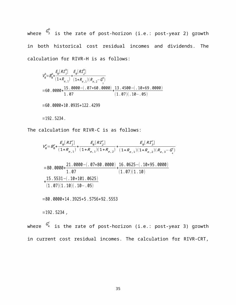
where G3h

is the rate of post-horizon (i.e.: post-year 2) growth in both historical cost residual

incomes and dividends. The calculation for RIVR-H is as follows:

20

V 0h=B0

h+E0 [ RI1

h ](1+Re , 1 )

+E0 [ RI 2

h ]

(1+Re , 1)( Re ,2−G3

h )

=60. 0000+15 . 0000−( .07∗60 . 0000)1 . 07 +

13 . 4500−( . 10∗69 .0000 )(1.07 )( .10−. 05)

=60. 0000+10 . 0935+122. 4299

=192 .5234 .

The calculation for RIVR-C is as follows:

V 0c=B0

c+E0 [RI 1

c ](1+Re , 1)

+E0 [RI 2

c ](1+Re , 1 )(1+Re ,2 )

+E0 [RI 3

c ]

(1+Re , 1)(1+Re , 2)( Re , 3−G4

c )

=80 .0000+21.0000−( . 07∗80. 0000 )1. 07

+16 .0625−( . 10∗95 .0000 )(1 .07 )(1 .10 )

+15 . 5531−( . 10∗101. 0625)(1. 07 )(1. 10)( . 10−. 05 )

=80. 0000+14 . 3925+5 .5756+92 .5553

=192 . 5234 ,

where G4c

is the rate of post-horizon (i.e.: post-year 3) growth in current cost residual incomes.

The calculation for RIVR-CRT, written in the form of expression (19) which links directly with

the RW model, is as follows:

21

V 0c , real , 0 = B0

c

+

E0[Y 1h

1+ p1−

ADEPN 1

1+p1+

p1 D0

1+ p1+( π1−p1 ) A0

c

1+p1−re , 1 B0

c]1+r e , 1

+

E0[Y 2h

Πk=1

2

(1+ pk )

−ADEPN 2

Πk=1

2

(1+ pk )

+p2 D1

Πk=1

2

(1+ pk )

+( π2− p2 ) A1

c

Πk=1

2

(1+pk )

−re , 2 B1

c

1+ p1 ]∏k=1

2

(1+re , k )

+

E0[Y 3h

Πk=1

3

(1+ pk )

−ADEPN 3

Πk=1

3

(1+ pk )

+p3 D2

Πk=1

3

(1+ pk )

+( π3− p3 ) A2

c

Πk=1

3

(1+pk )

−re , 3 B2

c

Πk=1

2

(1+ pk) ]∏k=1

2

(1+re , k )(re , 3−g4 )

.

= 80 .0000

+

15 . 00001 . 01

−(12.0000−10. 0000 )1 . 01

+( . 01∗40 .0000 )1. 01

+(8 .0000120. 0000

−. 01)∗120. 0000

1. 01−( . 059406∗80 .0000 )

1 . 059406

+

13 . 4500(1. 01)(1 .03 )

−(13 .5000−10. 9000 )(1.01 )(1 .03)

+( . 03∗40 . 0000)(1 . 01)(1. 03 )

+(5 .2125135 . 0000

−. 03)∗135 . 0000

(1. 01)(1 .03)−. 067961∗95 .0000

1 . 01(1. 059406 )(1 . 067961)

+

14 . 1225(1. 01)(1 .03 )2 −

(14 . 3063−11. 4450)(1 . 01)(1. 03 )2 +

( .03∗42 . 0000)(1. 01)(1 .03 )2 +

( . 03−. 03)∗143 .0625(1. 01)(1 . 03)2 −. 067961∗101 .0625

(1 . 01)(1 .03 )(1. 059406 )(1 . 067961)( . 067961−. 019417)

¿80 . 0000+14 . 3925+5 .5756+92. 5553

¿192 .5234 ,

where g4 is the rate of post-horizon (i.e.: post-year 3) growth in real current cost residual

incomes as expressed in real terms at the valuation date.

22

This example shows that proper application of the various valuation approaches to

internally consistent inputs will yield identical value estimates. Our prime purpose in presenting

this example is to illustrate errors that could be made in applying an inflation-adjusted

formulation of RIVR, and which could result in erroneous differences between value estimates

obtained from the historical cost and inflation-adjusted formulations of RIVR. Examples of

possible errors are considered below.

Incorrect assumption that current cost residual income grows at the same rate as historical cost residual income in year 3.

In the example, the growth rate in historical cost residual income is constant at 5% after year 2.

The growth rate in nominal and real current cost residual income is -17% in year 3 and is

constant at 5% after year 3. The growth rates in real current cost residual income as stated in real

terms at the valuation date are -19.4175% (=(1-0.17)/(1+0.03)-1) for year 3 and 1.9417%

(=(1+0.05)/(1+0.03)-1) after year 3. Consider the effect of an erroneous assumption that, after

year 2, nominal (and real) current cost residual incomes are expected to grow at the same rate as

historical cost residual incomes, and are therefore expected to grow at the constant rate of 5%

after year 2. (Consistent with this, real current cost residual incomes as stated in real terms at the

valuation date are now expected to grow at the rate of 1.9417% after year 2.) This erroneous

assumption gives a value estimate of 217.0561. (See the Appendix for detailed calculations). The

apparently innocuous assumption that the year 3 rate of growth in nominal historical cost residual

incomes can be applied to current cost residual incomes has given rise to a value estimate that is

about 12.7% higher than the correct value estimate of 192.5234 calculated above. In subsection

4.2, we consider more formally the potentially complicated nature of the relationship between the

23

rates of growth in nominal historical cost residual incomes and current cost residual incomes, and

highlight further the danger of assuming that the rates of growth are equal.

Inconsistency between the nominal and real rates for the cost of equity and the post-horizon growth rate.

Another potential pitfall is to make the apparently innocuous assumption that the real cost of

equity and the real rate of growth in post-horizon flows can be approximated by subtracting the

inflation rate from the nominal cost of equity and the nominal growth rate, respectively. This

yields estimated real costs of equity of 6% in year 1 and 7% thereafter (instead of 5.9406% and

6.7961%), and an estimated real post-horizon growth rate in real current cost residual incomes of

2% (instead of 1.9417%). The detailed calculations given in the Appendix show that these

apparently innocuous approximations within RIVR-CRT yield an incorrect value estimate of

185.9588, which is about 3.4% less than the correct value estimate of 192.5234.

Inconsistency (lack of articulation) between current cost holding gains, current cost depreciation and movements in the current cost book value of assets.

It should be noted that the proper application of a formulation of RIVR employing current cost

income should use forecasts that comply with the current cost version of CSR. This requires that

changes in successive current cost balance sheet values of equity should articulate with periodic

dividends and current cost incomes, inclusive of both holding gains and current cost depreciation.

Failure to obey this articulation will result in value estimates that erroneously differ from those

given by RIVR-H. The complicated nature of the required articulation, even within our

simplified example, illustrates how easy it would be to fall into such error.

24

In this subsection, by reference to a numerical example we have illustrated some of the

complications and errors that might result from attempts to refashion nominal historical cost-

based accounting data to a form appropriate for use within an inflation-adjusted formulation of

RIVR. In the next subsection, we use a formal model of the relationship between growth in

nominal historical cost residual incomes and current cost residual incomes to emphasise this

point.

4.2 A model of the relationship between growth in nominal historical cost residual incomes and growth in current cost residual incomes

We now explore analytically, in a simplified setting, the relationship between growth in historical

cost residual incomes and growth in current cost residual incomes (real or nominal).13 The setting

is as follows. An all-equity firm is created at time t, with an initial contribution of equity capital,

which is invested in its entirety in operating assets (i.e: Bt

h=At

h

). It is expected that the firm will

generate a constant pre-depreciation accounting rate of return of α , that reducing balance

depreciation at the rate d (where d<α ) will be applied, that the time t+s nominal historical cost

pre-tax income of At +s−1 (α−d ) will be taxed at the constant rate of τ , that the dividend payout

ratio will remain constant at κ , that all retained earnings will be invested in operating assets, and

that the nominal cost of equity will remain constant at Re . Under these assumptions,

Et [ RI t+ sh ]=A

t

h(1+G h)s−1(( α−d )(1−τ )−Re ), (24)

where Gh=( α−d )(1−τ )(1−κ ) is the constant rate of growth in both the historical cost book

value of equity and the historical cost residual income.

25

Now consider the situation if expectations are framed in terms of current cost residual

incomes, where the assumed constant rate of holding gains is π and where the depreciation rate

d is now applied to the current cost of assets. Current cost residual income, both nominal and

real, is expected to evolve as follows:

RI t+1c =A

t

h((α−d )(1−τ )−R e+π )

RI t+2c =A

t

h(1+Gh )((α−d )(1−τ )−Re+π )+ At

h π (π−d−Re )

RI t+3c =A

t

h(1+Gh )2((α−d )(1−τ )−Re+π )+ At

h π [(1+Gh )+(1+π−d )](π−d−R e )

RI t+4c =A

t

h(1+Gh )3((α−d )(1−τ )−Re+π )

+ At

h π [ (1+Gh)2+(1+Gh)(1+π−d )+(1+π−d )2 ](π−d−R e )

etc . .. . .

(25)

Generalising,

Et [ RI t +sc ]=A

t

h(1+Gh)s−1(( α−d )(1−τ )−R e+π )

+ At

h π [(1+Gh)s−1−(1+π−d )s−1

(1+Gh)−(1+π−d ) ](π−d−R e ) . (26)

As s increases, the first term on the right-hand side of (26) grows at the constant rate of Gh

, but

the second term grows at the more complex time-varying rate of:

(1+Gh )s−1−(1+π−d )s−1

(1+Gh )s−2−(1+π−d )s−2 − 1 . (27)

For Gh>π−d , the growth rate given by (27) asymptotes to G

h, and the overall growth rate in

current cost residual income asymptotes to Gh

; for Gh=π−d , by L'Hospital's rule, the term in

square brackets in (26) reduces in the limit to (s−1 )(1+Gh )s−2, and the growth rate in current

26

cost residual income asymptotes to Gh

; for Gh<π−d , the growth rate given by (27)

asymptotes to π−d , and the overall growth rate in current cost residual income also asymptotes

to π−d . These asymptotic growth rates have an intuitive interpretation. If growth in nominal

historical cost residual income is greater than or equal to the rate of current cost holding gains

(less depreciation), then the nominal historical cost growth rate dominates; in the event that

growth in nominal historical cost residual income is less than the rate of current cost holding

gains (less depreciation), then the holding gain term (net of depreciation) dominates. Note,

however, that these are rates to which current cost residual income growth will asymptote in the

long term, and it is not correct in general to use as the rate of growth in current cost residual

incomes the rate of growth in forecasts of historical cost residual incomes, or a simple transform

thereof. Table 2 illustrates the patterns of current cost residual income growth in the presence of

constant residual income growth for two different rates of current cost holding gains, π : 1%

(0.01) and 5% (0.05). Other parameters are as follows: A

t

h

= 100, α = 0.40, d = 0.20, τ = 0.25,

κ = 0.60, and the nominal cost of equity, Re , is 0.10. The parameters α , d, , τ and κ give

rise to a rate of growth in historical cost residual income of 6% (0.06):

Gh=( α−d )(1−τ )(1−κ )¿(0 . 40−0 .20)(1−0. 25 )(1−0 . 60)¿0 .06 .

For π = 0.01, the growth rate in current cost residual income reaches 0.036 after 5 years, 0.053

after 10 years, and 0.058 after 15 years. In contrast, where π takes a value of 0.05, which is

much closer to that of Gh

, the growth in current cost residual income takes a lot longer to

approximate to the rate of growth in historical cost residual income. Under this circumstance, the

27

growth rate in current cost residual income is -0.031 after 5 years, 0.018 after 10 years, and 0.044

after 15 years.

As can be seen from this simplified illustration, the theoretical link between growth in

historical cost residual income and growth in its current cost counterpart can be complex. If the

valuer of a company has access to a readily available estimate of growth in historical cost

residual incomes, the unnecessary and potentially complex task of correctly recasting this

estimate to a current cost basis is likely to create significant scope for error.

4.3 Summary

In previous sections, we have demonstrated that there is no need to work with an inflation-

adjusted formulation of RIVR. In this section, using both a numerical example and a model of

the relationship between growth in historical cost and current cost residual incomes, we have

illustrated the potentially complicated nature of adjustments that have to be made in transforming

the nominal historical cost-based inputs to RIVR into a form that could be used in inflation-

adjusted formulations of RIVR. On the basis of our analysis, we conclude that inflation

adjustment of RIVR is not only unnecessary, but is a likely source of complexity and error.

5. Conclusion

Inflation can have marked effects on both the appearance and the reality of corporate

profitability. An issue that has exercised many accountants and economists over the years is

whether these effects are of such a nature and magnitude as to require the wholesale

transformation of traditional accounting data before reliable inferences can be drawn. Until

28

recently, the literature on accounting-based valuation models has been silent on the questions of

whether and how such models should be written in inflation-adjusted form. However, a recent

study by Ritter and Warr (2002) claims that failure to deal with inflation within RIVR can lead to

under-valuation of firms, a point that has been echoed in Bradley and Jarrell (2003). Our paper

explores the issue of whether it is indeed necessary to adjust RIVR in order to deal properly with

inflation. We find that formulations of the RIVR based on a number of inflation-adjusted income

measures from prior literature, including a formulation of which the Ritter and Warr (2002)

model is a special case, are each no more correct and no less correct than the standard

formulation based on nominal historical cost residual incomes. We have therefore established

that inflation adjustment of RIVR, as advocated by Ritter and Warr (2002) is unnecessary. Any

theoretical superiority claimed for the inflation-adjusted residual income valuation model over

the standard nominal historical cost formulation, due for example to inclusion of gains from debt

in periods of inflation, is therefore illusory.

Any case for using inflation-adjusted forecasts must rest on the practical ground that such

forecasts are easier to obtain or more reliable or both. Only in economies experiencing high

inflation are inflation-adjusted income forecasts likely to be readily available. As we have

illustrated, in other settings the inflation adjustment of readily available forecasts of nominal

accounting numbers may well introduce unnecessary and undesirable complexity, and scope for

error.

We emphasise that we do not argue that the effects of inflation should be ignored in

framing forecasts for use in RIVR by, for example, assuming zero growth for flows that are

expected to grow in line with inflation. The estimation of post-horizon residual income growth

29

should take account not only of matters related to competitive advantage, but also of the impact

of inflation on expectations regarding accounting numbers, under whatever convention those

numbers are constructed. However, we emphasis that, as long as forecast flows are represented in

a consistent manner, a nominal historical cost formulation of RIVR is as correct as an inflation-

adjusted formulation.

30

AppendixCalculations relating to numerical example in Section 4

Incorrect assumption that current cost residual income grows at the same rate as historical cost residual income in year 3.

Consider the effect of an incorrect assumption that current cost residual incomes (and real current

cost residual incomes) grow at the constant rate of 5% after year 2. This gives an incorrect value

estimate of 217.0561, about 12.7% greater than the correct estimate of 192.5234:

V 0c=80 . 0000

+21 . 0000−(. 07∗80 . 0000)1 . 07

+16 . 0625−( .10∗95 .0000 )(1. 07 )( .10−. 05)

¿80 . 0000+14 . 3925+122. 6636¿217 . 0561.

The erroneous assumption that nominal (and real) current cost residual incomes grow at the

constant rate of 5% after year 2 is equivalent to assuming that real current cost residual incomes

as stated in real terms at the valuation date grow at the rate of 1.9417% after year 2. This

representation, based on expression (19), gives the same value estimate:

V 0c , real ,0 = 80 . 0000

+

15 . 00001 . 01

−(12.0000−10. 0000 )1 . 01

+( . 01∗40 .0000 )1. 01

+(8 .0000120. 0000

−. 01)∗120. 0000

1. 01−( . 059406∗80 .0000 )

1 . 059406

+

13 . 4500(1. 01)(1 .03 )

−(13 .5000−10. 9000 )(1.01 )(1 .03)

+( . 03∗40 . 0000)(1 . 01)(1. 03 )

+(5 .2125135 . 0000

−. 03)∗135 . 0000

(1. 01)(1 .03)−. 067961∗95 .0000

1 . 01(1. 059406 )( . 067961−. 019417 )

¿80 . 0000+14 . 3925+122. 6636

¿217 . 0561

31

Inconsistency between the nominal and real rates for the cost of equity and the post-horizon growth rate.

The assumption that the real cost of equity and the real rate of growth in post-horizon flows can

be approximated by subtracting the inflation rate from the nominal cost of equity and the nominal

growth rate, respectively, yields estimated real costs of equity of 6% in year 1 and 7% thereafter

(instead of 5.9406% and 6.7961%), and an estimated real post-horizon growth rate in real current

cost residual incomes of 2% (instead of 1.9417%). Use of these apparently innocuous

approximations within RIVR-CRT yields an incorrect value estimate of 185.9588, which is about

3.4% less than the correct value estimate of 192.5234. The calculation is as follows, based on

expression (19):

V 0c , real ,0 = 80 . 0000

+

15 . 00001 .01

−(12.0000−10. 0000 )1 . 01

+( . 01∗40 .0000 )1.01

+(8120

−. 01)∗120 .0000

1. 01−( .06∗80 . 0000 )

1 .06

+

13 . 4500(1. 01)(1 .03 )

−(13 .5000−10.9000 )(1. 01 )(1 .03)

+( . 03∗40 . 0000)(1 . 01)(1. 03 )

+(5 .2125135 .0000

−. 03)∗135 .0000

(1. 01)(1 .03)−. 07∗95 . 0000

1 .01(1. 06 )(1 .07 )

+

14 . 1225(1. 01)(1 .03 )2 −

(14 . 3063−11. 4450)(1 .01)(1.03 )2 +

( .03∗42 . 0000)(1. 01)(1 .03 )2 +

( . 03−. 03)∗143 .0625(1. 01)(1 .03)2 −. 07∗101.0625

(1 . 01)(1 .03 )(1. 06 )(1 .07 )(. 07−. 02)

¿80 .0000+14 . 3396+5 .3928+86 .2264=185 .9588 .

32

Notes

33

References

Bradley, M. and G. Jarrell. (2003). "Inflation and the constant growth valuation model: A

clarification." Working Paper, Duke University and University of Rochester.

Edwards, E. and P. Bell. (1961). The Theory and Measurement of Business Income, University of

California Press.

Edwards, J., Kay, J. and C. Mayer. (1987). The Economic Analysis of Accounting Profitability,

Oxford University Press.

Financial Accounting Standards Board. (1979). Statement of Financial Accounting Standards

No. 33: Financial Reporting and Changing Prices.

Francis, J., P. Olsson and D. Oswald. (2000). "Comparing the accuracy and explainability of

dividend, free cash flow, and abnormal earnings equity value estimates." Journal of

Accounting Research 38, 45-70.

Frankel, R. and C. Lee. (1998). "Accounting valuation, market expectation and cross-sectional

stock returns." Journal of Accounting and Economics 25, 283-319.

International Accounting Standards Committee. (1994). International Accounting Standard No.

29: Financial Reporting in Hyperinflationary Economies.

Lee, C., J. Myers and B. Swaminathan. (1999). "What is the intrinsic value of the Dow?" Journal

of Finance 54, 1693-1741.

Lundholm, R. and T. O'Keefe. (2001). "Reconciling Value Estimates from the Discounted Cash

Flow Model and the Residual Income Model." Contemporary Accounting Research, 18,

331-335.

34

Ritter, J., and R. Warr. (2002). "The decline of inflation and the bull market of 1982-1999."

Journal of Financial and Quantitative Analysis 37, 29-61.

Scapens, R. (1981). Accounting in an Inflationary Environment, 2nd edition, Macmillan.

35

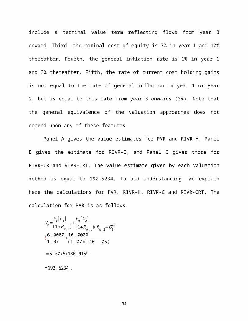
Table 1 Numerical example of the equivalence of formulations of RIVR based on historical cost and inflation-adjusted residual income measures

This example illustrates the consistency between valuation approaches based on dividends, historical cost residual incomes, and various inflation adjusted residual income measures. In this example, both dividends and historical cost residual incomes grow at the constant rate of 5% after year 2. Current cost residual incomes grow at this rate after year 3, but not in year 3. The cost of equity and inflation vary from year 1 to year 2, but each remains constant thereafter. These features are incorporated to facilitate exposition, and the general equivalence of the approaches does not depend upon them. Panel A: Value estimates based on dividends and historical cost (HC) residual incomes (PVR and RIVR-H)

Year 0 Year 1 Year 2 Year 3 Year 4 Year 0 Equity

TOTAL

Income statementHC income (excluding depreciation) (1) - 25.0000 24.3500 25.5675 26.8459HC depreciation (10%) (2) - -10.0000 -10.9000 -11.4450 -12.0173HC net income - 15.0000 13.4500 14.1225 14.8286Dividend - -6.0000 -10.0000 -10.5000 -11.0250HC retained earnings - 9.0000 3.4500 3.6225 3.8036Balance sheetHC Assets 100.0000 109.0000 114.4500 120.1725 126.1811Debt 40.0000 40.0000 42.0000 44.1000 46.3050HC Equity 60.0000 69.0000 72.4500 76.0725 79.8761

Cost of equity (3) - 0.07 0.10 0.10 0.10

Growth in dividends - - 0.6667 0.0500 0.0500Present value at year 0 of dividends - 5.6075 186.9159

(Terminal value) (6)192.5234

(PVR)

HC capital charge (4) 4.2000 6.9000 7.2450 7.6072HC residual income - 10.8000 6.5500 6.8775 7.2214Growth in HC residual incomes (5) - - -0.3935 0.0500 0.0500Present value at year 0 of HC residual incomes

- 10.0935 122.4299(Terminal value) (6)

60.0000 192.5234(RIVR-H)

36

37

Table 1 Numerical example of the equivalence of formulations of RIVR based on historical cost and inflation-adjusted residual income measuresPanel B: Value estimate based on current cost (CC) residual incomes (RIVR-C)

Year 0 Year 1 Year 2 Year 3 Year 4 Year 0 Equity

TOTAL

Income statementHC income (excluding depreciation) (1) - 25.0000 24.3500 25.5675 26.8459CC depreciation (1) (2) - -12.0000 -13.5000 -14.3063 -15.0216CC holding gain (8) 8.000 5.2125 4.2919 4.5065CC net income - 21.0000 16.0625 15.5531 16.3308Dividend - -6.0000 -10.0000 -10.5000 -11.0250CC retained earnings - 15.0000 6.0625 5.0531 5.3058Balance SheetCC Assets 120.0000 135.0000 143.0625 150.2156 157.7264Debt 40.0000 40.0000 42.0000 44.1000 46.3050CC Equity 80.0000 95.0000 101.0625 106.1156 111.4214

Cost of equity (3) - .07 .10 .10 .10

CC capital charge (4) 5.6000 9.5000 10.1062 10.6116CC residual income - 15.4000 6.5625 5.4469 5.7192Growth in CC residual incomes (7) - - -0.5739 -0.1700 0.0500Present value at year 0 of CC residual incomes

- 14.3925 5.5756 92.5553(Terminal value) (6)

80.0000 192.5234(RIVR-C)

38

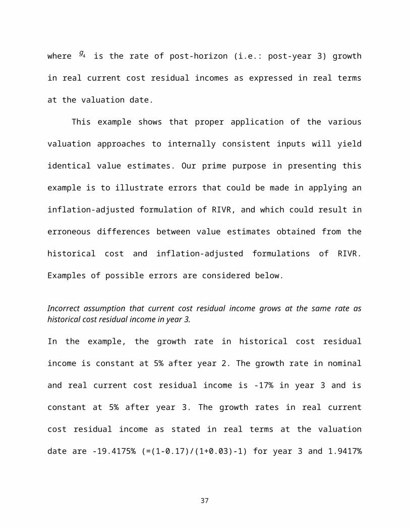
Table 1 Numerical example of the equivalence of formulations of RIVR based on historical cost and inflation-adjusted residual income measuresPanel C: Value estimates for real current cost (CC) residual incomes (RIVR-CR and RIVR-CRT)

Year 0 Year 1 Year 2 Year 3 Year 4 Year 0 equity

TOTAL

Income StatementHC income (excluding depreciation) (1) - 25.0000 24.3500 25.5675 26.8459CC depreciation (1) (2) - -12.0000 -13.5000 -14.3063 -15.0216CC holding gain (8) 8.000 5.2125 4.2919 4.5065Capital maintenance charge: Assets (9) -1.2000 -4.0500 -4.2919 -4.5065Capital maintenance charge: Debt (9) 0.4000 1.2000 1.2600 1.3230Real CC net income - 20.2000 13.2125 12.5212 13.1473Dividend - -6.0000 -10.0000 -10.5000 -11.0250Real CC retained earnings (11) - 14.2000 3.2125 2.0212 2.1223Balance SheetCC Assets 120.0000 135.0000 143.0625 150.2156 157.7264Debt 40.0000 40.0000 42.0000 44.1000 46.3050CC Equity 80.0000 95.0000 101.0625 106.1156 111.4214

Nominal cost of equity (3) - .07 .10 .10 .10General Inflation rate - .01 .03 .03 .03Real cost of equity (3) .059406 .067961 .067961 .067961

Base for real CC capital charge (4) - 80.8000 97.8500 104.0944 109.2991Real CC capital charge (4) - 4.8000 6.6500 7.0743 7.4281Real CC residual income - 15.4000 6.5625 5.4469 5.7192Growth in real CC residual income - - -0.5739 -0.1700 0.0500Present value of real CC residual incomes - 14.3925 5.5756 92.5553

(Terminal value) (6)80.0000 192.5234

(RIVR-CR)Real CC residual income in real terms as at year 0 (10)

- 15.2475 6.3083 5.0834 5.1821

Growth in real CC residual income in real terms as at year 0

- -0.586273 -0.194175 0.019417

Present value of real CC residual incomes in real terms as at year 0

- 14.3925 5.5756 92.5553(Terminal value) (6)

80.0000 192.5234(RIVR-CRT)

39

Notes to Table 1:1. HC denotes historical cost. CC denotes current cost.2. Depreciation is at the rate of 10% on a reducing balance basis, applied to the opening net book value of assets.3. The nominal cost of equity is allowed to vary between years 1 and 2, and remains constant at 10% from year 2 onwards. The real costs of equity for years 1

and 2, based on the inflation rates for years 1 and 2 of 1% and 3%, are calculated as follows: ((1.07)/(1.01)) - 1 = 0.059406; ((1.10)/(1.03)) - 1 = 0.067961.4. The historical cost capital charge is calculated by applying the cost of equity for the year to the opening historical cost book value of equity for the year. For

example, the capital charge for year 1 is 0.07 * 60.0000 = 4.2000. The current cost capital charge is calculated by applying the cost of equity for the year to the opening current cost book value of equity for the year. For example, the capital charge for year 1 is 0.07 * 80.0000 = 5.6000. The real current cost capital charge is calculated by applying the real cost of equity for the year to the opening current cost book value of equity as augmented at the rate of inflation for the year. For example, the capital charge for year 1 is 0.059406*(80.0000 * 1.01) = 0.059406* 80.8000 = 4.8000.

5. It is not true in general that the rate of growth in historical cost residual incomes is equal to that in dividends. This example is constructed such that the two items grow at the same rate after year 2.

6. All terminal value calculations reflect expected growth at a constant rate in perpetuity.The terminal value of dividends is calculated as follows: [10.0000/(0.10-0.05)]/1.07 = 186.9159.The terminal value of nominal historical cost residual incomes is calculated as follows: [6.5500/(0.10-0.05)]/1.07 = 122.4299.The terminal value of current cost residual incomes is calculated as follows: [5.4469/(0.10-0.05)]/[(1.07)(1.10)] = 92.5553. The same calculation applies for the terminal value of real current cost residual incomes, since nominal and real current cost residual incomes are identical to each other.The terminal value of real residual incomes as stated in real terms at the valuation date is calculated as follows:

[5.0834/(.067961-0.019417)]/[(1.059406)(1.067961)] = 92.5553.7. It is not true in general that the rate of growth in current cost residual incomes is equal to that of historical cost residual incomes. This example is

constructed such that the two items grow at the same rate after year 3. 8. In years 1 and 2, the current cost holding gains do not accrue at the rate of general inflation. From year 3 onwards, they accrue at the general rate of inflation

(=3%). The year 3 holding gain is 3% of 143.0625 = 4.2919.9. The capital maintenance charges are calculated by applying the general rate of inflation for the period to the beginning-of-period balances of the items in

question.10. The real CC residual income in real terms as at year 0 is calculated by dividing by the cumulative effect of inflation. For example, the figure for year 2 is

calculated as follows: 6.5625/(1.01)(1.03) = 6.3083. 11. Note that, because of the capital maintenance charge, real current cost retained earnings is not equal to the periodic change in the book value of equity.

40

Table 2 Illustration of patterns of growth in nominal historical cost residual income and current cost residual income

Year Nominal historical cost residual income

Current cost residual income (holding gain rate =1%)

Current cost residual income (holding gain rate =5%)

Level Growth Level Growth Level Growtht+1 5.000 6.000 10.000t+2 5.300 .060 6.070 .012 9.350 -0.065t+3 5.618 .060 6.199 .021 8.849 -0.054t+4 5.955 .060 6.381 .029 8.476 -0.042t+5 6.312 .060 6.610 .036 8.217 -0.031t+6 6.691 .060 6.881 .041 8.058 -0.019t+7 7.093 .060 7.193 .045 7.987 -0.009t+8 7.518 .060 7.543 .049 7.994 0.001t+9 7.969 .060 7.929 .051 8.073 0.010

t+10 8.447 .060 8.351 .053 8.217 0.018t+11 8.954 .060 8.809 .055 8.421 0.025t+12 9.491 .060 9.302 .056 8.680 0.031t+13 10.061 .060 9.832 .057 8.991 0.036t+14 10.665 .060 10.398 .058 9.353 0.040t+15 11.305 .060 11.003 .058 9.763 0.044

41

Note to Table 2:This table illustrates the behaviour of growth in historical cost residual incomes ( RI h

) and in current cost residual incomes (RI c), in

accordance with the following generating processes described in the text:Et [ RI t+ s

h ]=At

h(1+Gh)s−1(( α−d )(1−τ )−R e ) (24)

Et [ RI t+ sc ]=A

t

h(1+G h)s−1(( α−d )(1−τ )−R e+π )+ At

h π [ (1+Gh)s−1−(1+π−d )s−1

(1+Gh)−(1+π−d ) ](π−d−R e ) . (26)

As described in the text, the setting is as follows. An all-equity firm is created at time t, with an initial contribution of equity capital of At

h (=100), which is invested in its entirety in operating assets. The firm generates a constant pre-depreciation accounting rate of

return of α (=0.40), reducing balance depreciation is charged at the rate d (=0.20), historical cost pre-tax income is taxed at the rate of τ (=0.25), the dividend payout ratio is κ (=0.60), all retained earnings are invested in operating assets, and the nominal cost of

equity is constant at Re (=0.10). Two rates of current cost holding gains, π , are considered: 0.01 (1%) and 0.05 (5%). The rate of

growth in historical cost residual incomes, Gh

, is as follows:Gh=( α−d )(1−τ )(1−κ )¿(0 . 40−0 .20)(1−0. 25 )(1−0 . 60)¿0 .06 .

42

1 This condition is exactly met if the firm is expected to be wound up at some finite date in the

future, since after that date book value is zero.

2 Our exposition allows the cost of equity to vary over time. In practical applications, it is

commonly assumed that the cost of equity is constant, i.e., its term structure is flat.

3 We assume the firm's balance sheets contain only depreciable plant and equipment financed by

debt and equity, and this assumption is also made by RW. The assumption is less restrictive than

appearances might suggest. Assets such as inventories and real estate, which are not normally

subject to depreciation, can be thought of as special forms of depreciable asset. For such assets, the

depreciation rate can be taken to be zero until the asset is sold or otherwise disposed of, at which

time the depreciation rate is 100%. Likewise, a typical firm will have significant monetary liabilities

other than interest-bearing debt (notably amounts owed to suppliers); it will also have monetary

assets, such as cash balances and trade credit extended to customers. The concept of debt must

therefore be expanded to include monetary working capital items, with the rate of interest on these

items being set equal to zero.

4 This treatment is in line with that required by all of the inflation accounting standards that have

appeared in Anglo-Saxon countries, including Statement of Financial Accounting Standards No. 33.

An alternative way of motivating this treatment is to assume that all debt is issued on a floating-rate

basis.

5 This assumption is also made by RW. It should be noted however that all the arguments made in

this paper would apply equally to other ways of measuring changes in the value of a firm's assets,

such as by reference to realizable proceeds.

6 Further details on the real current cost income measure are provided in Edwards and Bell (1961,

chapter 8), Scapens (1981, chapter 6) and Edwards, Kay and Mayer (1987, chapter 5). The now

defunct Statement of Financial Accounting Standards No. 33 (Financial Accounting Standards

Board, 1979) required real current cost income to be presented as supplementary information within

U.S. financial statements.

7 The terms on the right-hand side of expression (11) correspond to items in the illustration

appearing in Appendix A of Schedule A of Statement of Financial Accounting Standards No. 33.

The first two terms taken together correspond to the 'loss from continuing operations adjusted for

changes in specific prices'. (In the illustration given in the standard, current cost income is

negative.) The third term corresponds to the 'gain from decline in purchasing power of net amounts

owed'. The fourth term corresponds to the 'increase in specific prices (current cost) of inventories

and property, plant, and equipment held during the year' less the 'effect of increase in general price

level' in respect of those items.

8 Of course, any anticipated decline in the purchasing power of money will be reflected in interest

charged on debt, and deducted as an expense in arriving at Y t+ sh

.

9 This is so because the last term, pt+ s B t+s−1c

, is not reflected in the change in book value between

time t+s-1 and time t+s.

10 The assumption that the extra depreciation charge is expected to increase at the general rate of

inflation is a restrictive one. A set of circumstances under which it would hold is as follows. First,

the firm is in steady state with a seasoned stock of identical depreciable assets of varying vintage

such that the annual outlay on replacement is equal to the current cost depreciation. (The method

used to depreciate the assets is of no consequence.) Second, the rate of change in the current

replacement cost of the assets remains equal to the (constant) rate of general inflation. If inflation

were time-varying and current cost depreciation increased in step with inflation, its historical cost

counterpart would not do so, and neither would the extra depreciation charge (the difference

between the two).

11 This is consistent with RW's assumption that the extra depreciation charge (ADEPN) rises in line

with general inflation.

12 However, even in a hyperinflationary economy, RIVR calculations based on nominal historical

cost residual incomes should, if done properly, yield the same value estimates as those obtained

using inflation-adjusted residual incomes.

13 Recall from Section 2 that real current cost residual income, RI c , real, is equal to nominal current

cost residual income RI c.