CONSERVATION ECOLOGY AND PHYLOGENETICS OF THE INDUS RIVER DOLPHIN
260
CONSERVATION ECOLOGY AND PHYLOGENETICS OF THE INDUS RIVER DOLPHIN (PLATANISTA GANGETICA MINOR) Gillian T. Braulik A Thesis Submitted for the Degree of PhD at the University of St. Andrews 2012 Full metadata for this item is available in Research@StAndrews:FullText at: http://research-repository.st-andrews.ac.uk/ Please use this identifier to cite or link to this item: http://hdl.handle.net/10023/3036 This item is protected by original copyright This item is licensed under a Creative Commons License
Transcript of CONSERVATION ECOLOGY AND PHYLOGENETICS OF THE INDUS RIVER DOLPHIN

CONSERVATION ECOLOGY AND PHYLOGENETICS OF THEINDUS RIVER DOLPHIN (PLATANISTA GANGETICA MINOR)
Gillian T. Braulik
A Thesis Submitted for the Degree of PhDat the
University of St. Andrews
2012
Full metadata for this item is available inResearch@StAndrews:FullText
at:http://research-repository.st-andrews.ac.uk/
Please use this identifier to cite or link to this item:http://hdl.handle.net/10023/3036
This item is protected by original copyright
This item is licensed under aCreative Commons License

Conservation Ecology and Phylogenetics of the
Indus River dolphin (Platanista gangetica minor)
Gillian T. Braulik
This thesis is submitted in partial fulfilment for the degree of
Doctor of Philosophy at the
University of St Andrews
March 2012

2
Thesis Declaration
1. Candidate’s declarations: I, Gillian T. Braulik, hereby certify that this thesis, which is approximately 75,000 words in length, has been written by me, that it is the record of work carried out by me and that it has not been submitted in any previous application for a higher degree. I was admitted as a research student in October, 2006 and as a candidate for the degree of PhD in October, 2007. The higher study for which this is a record was carried out in the University of St Andrews between 2006 and 2011. Date: Signature of Candidate: 2. Supervisor’s declaration: I hereby certify that the candidate has fulfilled the conditions of the Resolution and Regulations appropriate for the degree of PhD in the University of St Andrews and that the candidate is qualified to submit this thesis in application for that degree. Date: Date: Signature of Supervisor: Signature of Supervisor: 3. Permission for electronic publication: In submitting this thesis to the University of St Andrews I understand that I am giving permission for it to be made available for use in accordance with the regulations of the University Library for the time being in force, subject to any copyright vested in the work not being affected thereby. I also understand that the title and the abstract will be published, and that a copy of the work may be made and supplied to any bona fide library or research worker, that my thesis will be electronically accessible for personal or research use unless exempt by award of an embargo as requested below, and that the library has the right to migrate my thesis into new electronic forms as required to ensure continued access to the thesis. I have obtained any third-party copyright permissions that may be required in order to allow such access and migration, or have requested the appropriate embargo below. Access to printed copy and electronic publication of thesis through the University of St Andrews. Date: Date: Date: Signature of Candidate: Signature of Supervisor: Signature of Supervisor:

An Indus dolphin breaks the surface in view of a barrage. Photo credit: Aftab Rana, Adventure Foundation Pakistan

Table of Contents ABSTRACT ......................................... ............................................................... 14
ACKNOWLEDGEMENTS................................... ........................................................ 15
CHAPTER 1 - GENERAL INTRODUCTION .................. ............................................. 21
1.1 SOUTH ASIAN RIVER DOLPHINS ........................................................... 21
1.1.1 Other River Dolphin Species and Populations......................... 22
1.2 THE INDUS RIVER .............................................................................. 23
1.2.1 Indus River Mega-fauna .......................................................... 26
1.3 PREVIOUS DOLPHIN RESEARCH .......................................................... 27
1.4 HISTORICAL INFORMATION ON INDUS RIVER DOLPHINS ......................... 27
1.4.1 Historical Distribution .............................................................. 27
1.4.2 Historical Abundance .............................................................. 30
1.5 DEVELOPMENT OF THE INDUS BASIN IRRIGATION SYSTEM .................... 30
1.5.1 Barrage Construction .............................................................. 30
1.5.2 Water Diversion ...................................................................... 34
1.6 CURRENT STATUS OF THE INDUS RIVER DOLPHIN ................................ 35
1.6.1 Present Distribution................................................................. 35
1.6.2 Present Abundance ................................................................ 36
1.6.3 Encounter Rate ....................................................................... 38
1.6.4 IUCN Red List Assessment ..................................................... 38
1.7 HABITAT USE ..................................................................................... 40
1.8 BEHAVIOUR ....................................................................................... 41
1.9 LIFE HISTORY .................................................................................... 42
1.9.1 Growth .................................................................................... 42
1.9.2 Sexual Dimorphism ................................................................. 42
1.9.3 Sexual Maturity ....................................................................... 43
1.9.4 Calving.................................................................................... 43
1.10 ECHOLOCATION ................................................................................. 44
1.11 DIET ................................................................................................. 45
1.12 THREATS AND MANAGEMENT .............................................................. 45
1.12.1 Dolphin Hunting ...................................................................... 45
1.12.2 Pollution .................................................................................. 47

5
1.12.3 Fisheries Interactions .............................................................. 48
1.12.4 Canal Entrapment ................................................................... 49
1.12.5 Downstream Migratory Attrition ............................................... 49
1.12.6 Freshwater .............................................................................. 51
1.13 OBJECTIVES OF THIS STUDY ............................................................... 52
1.14 REFERENCES .................................................................................... 52
CHAPTER 2 - ABUNDANCE OF INDUS RIVER DOLPHINS ESTIM ATED USING
MARK-RECAPTURE FROM TANDEM VESSEL SURVEYS IN 2006 . ....................... 64
2.1 INTRODUCTION ............................................................................. 65
2.1.1 Challenges to Survey Design on the Indus River .................... 65
2.1.2 Indus River Dolphin Surveys ................................................... 67
2.2 METHODS ....................................................................................... 68
2.2.1 Study Site ............................................................................... 68
2.2.2 Field Survey Methods ............................................................. 68
2.2.3 Meeting Model Assumptions ................................................... 71
2.2.4 Identification of Matched Groups............................................. 73
2.2.5 Abundance Estimation ............................................................ 74
2.2.6 Availability Bias ....................................................................... 77
2.2.7 Bias in Group Size Estimates .................................................. 78
2.2.8 Trends in Abundance .............................................................. 78
2.3 RESULTS ........................................................................................ 79
2.3.1 Survey Summary .................................................................... 79
2.3.2 Identification of Matched and Missed Dolphin Groups ............. 81
2.3.3 Estimation of Abundance ........................................................ 83
2.3.4 Availability Bias ....................................................................... 88
2.3.5 Group Size Bias ...................................................................... 89
2.3.6 Trends in Abundance .............................................................. 92
2.4 DISCUSSION .................................................................................. 94
2.4.1 Survey Design ........................................................................ 94
2.4.2 Potential for Bias in Abundance Estimate ............................... 94
2.4.3 Abundance and Encounter Rate ............................................. 97
2.4.4 Trends in Abundance .............................................................. 99
2.5 REFERENCES .............................................................................. 100

6
CHAPTER 3 - CAUSES AND DYNAMICS OF INDUS RIVER DOL PHIN RANGE
COLLAPSE ......................................... ............................................................. 107
3.1 INTRODUCTION ........................................................................... 108
3.2 METHODS ..................................................................................... 110
3.2.1 Last Dolphin Sighting Date .................................................... 111
3.2.2 Identifying the Causes of Range Decline .............................. 114
3.3 RESULTS ...................................................................................... 119
3.3.1 Interview Surveys ................................................................. 119
3.3.2 Last Dolphin Sighting Date .................................................... 120
3.3.3 Dynamics of Range Decline .................................................. 123
3.3.4 Causes of Range Decline ..................................................... 124
3.4 DISCUSSION ................................................................................ 131
3.4.1 Dynamics of Range Decline .................................................. 131
3.4.2 Causes of Range Decline ..................................................... 133
3.4.3 Implications for the Future..................................................... 137
3.5 REFERENCES .............................................................................. 138
CHAPTER 4 - HABITAT USE BY INDUS RIVER DOLPHINS IN THE LOW WATER
SEASON ...................................................................................................... 145
4.1 INTRODUCTION ........................................................................... 146
4.2 METHODS ..................................................................................... 147
4.2.1 Data Sets .............................................................................. 147
4.2.2 Habitat Models ...................................................................... 154
4.2.3 Habitat Preference ................................................................ 157
4.3 RESULTS ...................................................................................... 158
4.3.1 Data Summary ...................................................................... 158
4.3.2 Available Habitat ................................................................... 159
4.3.3 Dolphin Presence ................................................................. 162
4.3.4 Habitat Models ...................................................................... 162
4.3.5 Habitat Preference ................................................................ 168
4.4 DISCUSSION ................................................................................ 169
4.4.1 Available Habitat ................................................................... 169
4.4.2 Habitat Selection ................................................................... 169
4.4.3 Model Performance............................................................... 172

7
4.4.4 Potential Biases or Improvements to Habitat Models ............ 173
4.4.5 Conservation Implications ..................................................... 174
4.5 REFERENCES .............................................................................. 175
CHAPTER 5 - HIGH LINEAGE DIVERGENCE AND LOW GENETIC DIVERSITY IN
GEOGRAPHICALLY ISOLATED POPULATIONS OF SOUTH ASIAN RIVER
DOLPHIN ...................................................................................................... 182
5.1 INTRODUCTION ........................................................................... 183
5.1.1 Platanista Nomenclature and Taxonomic Studies ................. 184
5.1.2 Formation of the Indus and Ganges River Systems .............. 185
5.1.3 Phylogenetic Study and Conservation .................................. 186
5.2 METHODS ..................................................................................... 187
5.2.1 Sample Origin ....................................................................... 187
5.2.2 Sample Collection ................................................................. 187
5.2.3 Genetic Diversity ................................................................... 192
5.2.4 Population Differentiation ...................................................... 194
5.2.5 Phylogeographic Patterns ..................................................... 194
5.2.6 Divergence Time Estimation ................................................. 196
5.3 RESULTS ...................................................................................... 197
5.3.1 Molecular Diversity................................................................ 197
5.3.2 Population Differentiation ...................................................... 202
5.3.3 Divergence Time ................................................................... 203
5.4 DISCUSSION ................................................................................ 204
5.4.1 Lack of Variability .................................................................. 204
5.4.2 Divergence and Speciation ................................................... 206
5.4.3 Conclusions .......................................................................... 210
5.5 REFERENCES .............................................................................. 211
CHAPTER 6 – GENERAL DISCUSSION .................... ............................................. 222
6.1 THESIS SYNTHESIS .......................................................................... 222
6.2 ABUNDANCE ESTIMATION ................................................................. 222
6.3 PLATANISTA SPECIATION .................................................................. 226
6.4 INDUS DOLPHIN HABITAT AND ENVIRONMENTAL FLOWS ..................... 227

8
6.4.1 Dams .................................................................................... 230
6.5 CLIMATE CHANGE ............................................................................ 231
6.6 PROTECTED AREAS ......................................................................... 232
6.7 MORTALITY MONITORING ................................................................. 234
6.8 MOVEMENT OF DOLPHINS THROUGH BARRAGES ............................... 236
6.9 DOLPHIN TRANSLOCATION ............................................................... 238
6.10 CONCLUDING REMARKS ................................................................... 242
6.11 REFERENCES .................................................................................. 243
APPENDIX I – INTERVIEW QUESTIONNAIRE ........................................................ 250
APPENDIX II – LOCAL EVENTS CALENDAR USED TO REFINE DATES OF
HISTORICAL DOLPHIN SIGHTINGS ....................................................................... 251
APPENDIX III – DETAILS OF CURRENT AND FORMER FRAGMENTS OF INDUS
DOLPHIN HABITAT .................................................................................................. 252
APPENDIX IV – CITES IMPORT AND EXPORT PERMITS ...................................... 254
APPENDIX V - PLATANISTA ANCIENT DNA EXTRACTION LABORATORY
PROTOCOLS ...................................................................................................... 258

List of Tables and Figures
List of Figures
Figure 1.1 The geography and river systems of South Asia.
Figure 1.2 View of the Indus River looking downstream from Kotri barrage.
Figure 1.3 The Indus River system, and the location of irrigation barrages and
dams.
Figure 1.4 Distribution of the Indus (above left) and Ganges (above right) River
dolphins in the 1870’s. Replicated from Anderson (1879).
Figure 1.5 Upstream view of Sukkur Barrage.
Figure 1.6 Aerial photo of the Indus River (flowing from right to left) at Sukkur
barrage, illustrating the canals, barrage and change in flow above and
below a barrage.
Figure 1.7 Timing of Indus dolphin habitat subdivision, and the decline in size of the
longest portion of unfragmented Indus dolphin habitat.
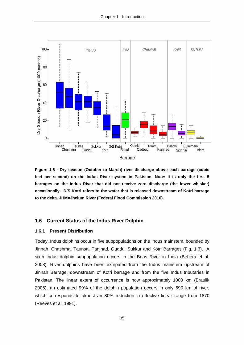
Figure 1.8 Dry season (October to March) river discharge above each barrage
(cubic feet per second) on the Indus River system in Pakistan.
Figure 1.9 Abundance and encounter rate of Indus River dolphins in each
subpopulation in 2006.
Figure 1.10 Twenty kilometres moving average encounter rate of Indus River
dolphins between Jinnah and Kotri Barrages.
Figure 2.1 Map of the Indus River system illustrating the barrages that form the
boundaries between the five subpopulations.
Figure 2.2 Frequency of dolphin radial sighting distances.
Figure 2.3 Distance between the exact geographic positions of potentially matched
dolphin groups.
Figure 2.4 Frequency of missed and matched sightings by a) group size and b)
river state between Chashma and Taunsa barrages.
Figure 2.5 Frequency of missed and matched sightings by a) group size and b)
river state between Guddu and Sukkur barrages.
Figure 2.6 Difference in group size estimates for matched sightings.

10
Figure 2.7 The time taken to estimate the number of dolphins in a group according
to group size.
Figure 2.8 Natural logarithm of Indus River dolphin (Platanista gangetica minor)
direct counts recorded between Guddu and Sukkur barrages between
1974 and 2008.
Figure 3.1 Map of the lower Indus River system, with rivers and barrages named,
and each extant or extirpated Indus dolphin subpopulation numbered.
Figure 3.2 Proportion of respondents that had seen Indus dolphins according to
age group.
Figure 3.3 Spatial and temporal dynamics of the Indus dolphin range decline.
Figure 3.4 Characteristics of river sections where river dolphins are present and
where they have been extirpated.
Figure 3.5 Probability that an Indus dolphin subpopulation is extant according to
proximity to the edge of the former range and the median dry season
discharge (cubic feet per second).
Figure 3.6 Relationship between the number of years since a dolphin was sighted
and a) subpopulation distance from historical range edge, and b)
median dry season discharge, the two significant explanatory variables
retained in quasi-Poisson GLM models of the temporal pattern of Indus
dolphin range decline.
Figure 3.7 Probability that an Indus dolphin subpopulation is extant with increasing
time of isolation
Figure 4.1 Illustration of a typical river cross-section and summary data calculated.
Figure 4.2 Illustration of two 5km segments of the Indus River and the river
hydrogeomorphic features recorded.
Figure 4.3 Boxplots of channel geometry and river geomorphology characteristics
in different sections of the Indus River.
Figure 4.4 Probability of Indus dolphin presence in relation to total channel cross-
sectional area (m2).

11
Figure 4.5 Predicted Indus dolphin abundance in relation to channel cross-
sectional area (m2).
Figure 4.6 Probability of Indus dolphin presence in relation to channel cross-
sectional area below 1m in depth.
Figure 4.7 Delta AIC (presence) and Delta QAIC (abundance) scores for models
that explain dolphin presence and abundance based on channel cross-
sectional area below different threshold depths.
Figure 4.8 Probability of Indus dolphin presence according to river width measured
in 1km river segments.
Figure 4.9 Observed and expected number of cross-sections with dolphins present
according to channel cross-sectional area and channel top width.
Figure 4.10 Illustrations of two actual channel cross-sections with the same total
cross-sectional area but great differences in the area below 1m in depth.
Figure 5.1 The Indus, Ganges, Brahmaputra and Karnaphuli River systems
Figure 5.2 Median-joining network based on complete MtDNA control region
haplotypes for the cetacean Family Platanista.
Figure 5.3 Median-joining network based on partial cytochrome b sequence
haplotypes for the cetacean Family Platanista.
Figure 5.4 Maximum likelihood bootstrap consensus tree representing the
evolutionary history of Platanista.
Figure 5.5 Elevation of the Indus-Ganges River system drainage divide and of
rivers near the divide
List of Tables
Table 1.1 Chronology of barrage construction within the historical range of the
Indus dolphin
Table 1.2 Published counts of Indus River dolphins between Guddu and Sukkur
barrages (subpopulation 4), Taunsa and Guddu barrages
(Subpopulation 3) and Chashma and Taunsa barrages (Subpopulation
2) reproduced from Braulik et al (2006).

12
Table 2.1 Summary of direct counts recorded in the Indus dolphin range-wide
abundance survey in 2006.
Table 2.2 Comparison of difference distance thresholds used to identify matched
and missed sightings.
Table 2.3 Summary of Indus dolphin subpopulation abundance estimation.
Table 2.4 Sighting availability of Indus dolphin groups.
Table 2.5 Comparison of direct counts of Indus River dolphin subpopulations
recorded in 2001 and 2006 using identical survey methods.
Table 2.6 Comparison of dolphin encounter rates on the Indus River with those
recorded for other river dolphins.
Table 3.1 Indus dolphin sighting records in the Punjab rivers since the 1920s.
Table 3.2 Details of extant and extirpated Indus dolphin subpopulations.
Table 3.3 Summary of spatial range decline model outputs.
Table 3.4 Summary of temporal range decline model outputs.
Table 4.1 Hydrogeomorphic and spatial characteristics described for each river
segment and included in Generalised Linear Models.
Table 4.2 Summary of channel geometry recorded at cross-sections, and river
geomorphology characteristics in different sections of the Indus River.
Table 4.3 Channel shape characteristics retained in final GLM models of dry
season Indus dolphin presence and abundance listed in order of
significance.
Table 4.4 Characteristics of river hydrogeomorphology measured over three
scales that were retained in final GLM models of dry season Indus
dolphin presence and abundance listed in order of significance.
Table 5.1 Platanista samples collected for this study with details of the year and
location of origin, museum and record number.
Table 5.2 Platanista sp. complete mtDNA control region sequences from GenBank
used in this study.

13
Table 5.3 Platanista sp. Cytochrome b sequences from GenBank used in the
current study.
Table 5.4 Nucleotide and haplotype diversity in MtDNA control region samples
from the Indus and Ganges-Brahmaputra rivers.
Table 5.5 Haplotypes identified in a 458bp portion (shaded grey), and in the entire
(858bp) Mitochondrial control region in two geographically isolated
populations of Platanista.
Table 5.6 Haplotypes and variable sites in a 541bp portion of the cytochrome b
gene from 20 Platanista sequences available on GenBank or as
unpublished data.

Abstract
The historical range of the Indus River dolphin has declined by 80% since the 19th
century and has been fragmented into 17 river sections by construction of irrigation
barrages. Dolphin sighting and interview surveys showed that river dolphins persist in
six river sections, have been extirpated from ten, and are of unknown status in the
remaining section. Logistic regression and survival modelling showed that low dry
season river discharge was the primary factor responsible for the Indus dolphins range
decline.
Abundance of the three largest Indus dolphin subpopulations was estimated using
tandem vessel-based direct counts, corrected for missed animals using conditional-
likelihood capture-recapture models. The entire subspecies was estimated to number
between 1550-1750 in 2006. Dolphin encounter rates within the Guddu- Sukkur
subpopulation (10.35/km) were the highest reported for any river dolphin and direct
counts suggest that this subpopulation may have been increasing in abundance since
the 1970s when hunting was banned.
The dry season habitat selection of Indus dolphins was explored using Generalised
Linear Models of dolphin distribution and abundance in relation to river geomorphology,
and channel geometry in cross-section. Channel cross-sectional area was shown to be
the most important factor determining dolphin presence. Indus dolphins avoided
channels with small cross-sectional area <700m2, presumably due to the risk of
entrapment and reduced foraging opportunities.
The phylogenetics of Indus and Ganges River dolphins was explored using
Mitochondrial control region sequences. Genetic diversity was low, and all 20 Indus
River dolphin samples were identical. There were no haplotypes shared by Indus and
Ganges River dolphins, phylogenetic trees demonstrated reciprocal monophyletic
separation and Bayesian modelling suggested that the two dolphin populations
diverged approximately 0.66 million years ago.
Declining river flows threaten Indus dolphins especially at the upstream end of their
range, and it is important to determine how much water is required to sustain a dolphin
population through the dry season. Fisheries interactions are an increasing problem
that will be best addressed through localised, community-based conservation activities.

15
Acknowledgements
Chapter 2 - The 2006 dolphin survey expedition covered a significant portion of
Pakistan’s territory, passing through remote and often insecure areas in three
Provinces. As much as a scientific endeavour it was a logistical and security operation
and its success is attributed to the collaboration and facilitation of numerous different
organisations and government departments in Pakistan, in particular: Sindh Wildlife
Department, Punjab Wildlife Department, NWFP Wildlife Department, Adventure
Foundation Pakistan, WWF-Pakistan, Ministry of Environment, Sindhi tribal leaders, the
Punjab, Sindh and NWFP Police Forces, Punjab and Sindh Irrigation Departments,
Water and Power Development Authority (WAPDA) and the staff at Jinnah, Chashma,
Taunsa, Guddu, Sukkur and Kotri Barrages. The logistical support that underpinned the
success of the expedition was ably undertaken by the expert volunteers at the
Adventure Foundation Pakistan: Rauf Ahmed, Mubashar Azam, Mohammad Abuhu,
Aftab Rana and Imdad. Huge credit is due to the scientific teams that worked long
hours in hot, remote and sometimes dangerous situations: Abdul Haleem, Abdul
Razzaq, Ashfaq Khan, Albert Reichert, Babar Hussain, Khalil Kundi, Kunwer Javed,
Malik Farooq Ahmad, Mohammad Saleem Chaudhry, Rafiq Rajput, Samiullah Khan,
Syed Athar Hussain, Tahir Ehsan, Uzma Khan, Zafar Ali, Shabir Ahmad, Muhammad
Hamid, Iqbal Khaskheli, Amir Buksh Bullo and Zahid Bhatti. Valuable statistical input
was provided by Sharon Hedley.
The survey was funded by the Pakistan Wetlands Programme of WWF-Pakistan, that
itself received funding from UNDP-GEF and the Embassy of the Kingdom of the
Netherlands, the Whale and Dolphin Conservation Society – UK and WWF-Pakistan.
ASTER Satellite images were provided by NASA specifically for this project and were
prepared by Raza Shah and Urooj Saeed.
Chapter 3 - I would like to extend thanks to my colleagues Uzma Noureen, Masood
Arshad and Najam ul-Huda who travelled with me for ten days around Punjab
conducting interviews with numerous colourful characters. In every town visited the
fishing community was located, usually a very poor settlement of grass houses and
charpai’s, and we requested to speak with the oldest fishermen present. Old men were
wheeled out, carried out and hobbled out of their houses to speak with us. They told
us fascinating stories of a bygone era. Some were sweet, some were cantankerous,

16
some were grandfatherly, and all were memorable. In addition to information on the
decline of the Indus dolphin, we also collected information on the decline of river otters,
gharial and crocodile, and the illegal trade in freshwater turtles. Ahmad Khan, Masood
Arshad and Richard Garstang facilitated and encouraged the interview surveys and
had faith that they would show interesting results. The initial idea for this work grew
from discussions with Sam Turvey about the decline of the Yangtze River dolphin. The
survey was funded by the Pakistan Wetlands Programme. The Marine Mammal
Commission supported my attendance at the 19th Biennial Conference of the Society of
Marine Mammalogy in Tampa, Florida, where I presented the information from this
chapter, “Causes and dynamics of Indus River dolphin range decline” and received the
J. Stephen Leatherwood Memorial Award for conservation of marine mammals in
South and Southeast Asia.
Chapter 4 - The dolphin survey data used in this chapter was collected in 2001 and
2006 by a large number of individuals from numerous organisations including Sindh
Wildlife Department, Punjab Wildlife Department, NWFP Wildlife Department,
Zoological Survey Department and WWF-Pakistan. The cross-section study was
devised and conducted by Albert Reichert with assistance from Tahir Ehsan and the
participation of many members of the 2006 dolphin survey team. Technical advice and
guidance on the geomorphic classification and cross-section calculations was provided
by Albert Reichert, preliminary classification of river geomorphology was conducted by
Samiullah Khan at PWP and Jason Alexander at the US Geological Survey provided
invaluable assistance and review of the geomorphic aspects of the chapter. Vital
statistical guidance was provided by Mike Lonergan at SMRU. Valuable reviews of this
chapter were contributed by Mike Lonergan, Albert Reichert, Jason Alexander, Uzma
Khan, Gianna Minton and Tim Collins. Satellite images were generously provided by
Michael Abrams at NASA. Funding was provided by the Whale and Dolphin
Conservation Society, WWF-Pakistan and the Ministry of Environment’s Pakistan
Wetlands Programme, which receives its support from UNDP GEF and the Royal
Netherlands Embassy.
Chapter 5 - For facilitating access to museum specimens I would like to thank Doris
Moerike at the Staatliches Museum für Naturkunde Stuttgart, Richard Sabin at the
British Museum of Natural History, Martin Milner at the Bell-Pettigrew Museum at the
University of St. Andrews, Mathew Lowe and Robert Asher at the Cambridge University

17
Museum of Zoology, Andrew Kitchener and Jerry Herman at the National Museums of
Scotland collections in Edinburgh, Uzma Khan at WWF-Pakistan, Kelly Robertson at
the NMFS, South West Fisheries Science Center, Tom Jefferson and Bill Perrin. The
laboratory work was conducted by Ross Barnett in collaboration with Rus Hoelzel at
the University of Durham Ancient DNA Laboratory. Jeff Graves in the School of Biology
was my advisor for this chapter, his reviews were extremely helpful, his rapid response
enormously appreciated; Jeff you are a pleasure to work with. I would particularly like
to thank Nicola Hodgins for her assistance in facilitating funding which was provided by
the Whale and Dolphin Conservation Society.
Financial support during all my studies was provided by the British Federation of
Women Graduates, the University of St. Andrews, and the US Marine Mammal
Commission.
It was Brian Smith who first introduced me to river dolphins when he encouraged me to
join him on a survey of the Karnaphuli River in eastern Bangladesh in early 1999. I was
captivated by Bangladesh and the river dolphins and that survey started me off along
this current path. My brother Rich was the one who encouraged me to go to Pakistan
in the first place, having spent two years volunteering with WWF-Pakistan conducting
raptor surveys in the Himalaya and Karakoram mountains. I doubt I would have ever
gone to Pakistan without this introduction, and it is unfortunate that our stays never did
overlap. Richard Garstang, Conservation Advisor with WWF-Pakistan answered my
original letter, and over the following 12 years has facilitated, encouraged and
supported my work. Nobody loves wildlife, or Pakistan, more than Richard. Randy
Reeves was the one who kept me going. His quiet and constant support and
encouragement gave reassurance that someone in the outside world was paying
attention and that what I was doing had value outside Pakistan as well.
WWF-Pakistan gave me a home and a family in Pakistan, have been supportive of my
work, and tolerant of my mistakes. I have spent months in the field with many good
friends, and hope that there will be many more expeditions to come. I have so many
friends and colleagues in Pakistan to thank: Samiullah Khan, Zafar Ali, Mubashar
Azam, Uzma Noureen, Uzma Khan, Masood Arshad, Ahmad Khan, Ghulam Akbar,
Ejaz Ahmed, Ali Habib, Mehjabeen Abidi-Habib, Hussain Bux Bhagat, Mumtaz Malik,
Imtiaz Tajwer, Khalil Kundi, Tahir Ehsan, Nabila Khan, Shafaq Masood, Umer Waqas,

18
Babar Hussain, Rafiq Rajput, Najam ul-Huda, Abdul Haleem, Imdad, Yakoob, Khalid,
Anna and Mark Pont, and Melissa Payson to name but a few.
At the beginning of this PhD project, I spent 1 torturous year waiting in Islamabad for a
permit from the Home Department to allow me to travel to the field. Doug and Humera
I can never thank you enough for putting me in touch with Salman who finally solved
the problem in less than a week. Salman, I am forever grateful to you. Despite my
permit, once in the field conducting the range wide survey described in Chapter 2, I
was detained at Dera Ghazi Khan and kept under house arrest for a week with my own
troop of black burka-clad female ninja guards present night and day. When we were
released it was on the condition that we not survey the remaining 300 km of river in
Punjab because of security concerns (specifically the ‘Bosun Gang’). We used cranes
to put the boats on trucks and drove with an escort of police vehicles with mounted
machine guns to Sindh where the survey resumed. That is why survey coverage of the
Taunsa to Guddu river section (subpopulation 3) was incomplete in 2006. In general,
the Pakistani authorities have been very tolerant of the dolphin survey expeditions that
we have conducted over the years, they have cooperated with us to minimize the risks
in tribal and insecure areas while attempting to allow us to do our job, despite their lack
of understanding about what we were doing or why we doing it.
My friends in St. Andrews: Alice, Sol, Theoni, Danielle, Becky, Sonja, Marjolaine, Rene,
Inez, Aaron, Gwen, Cormac, Sanna, Tess and so many more made life in St. Andrews
a great deal of fun. My friends in Rwanda: Katie and Glenn, Barbara, Katie K, Maria,
Christelle, Catherine, Thierry, and Christina, gave me a support team, even though
dolphins, the ocean, Pakistan, and the university were a million miles away. Gianna,
thank you for your support, you and your project in Sarawak are an inspiration. Moth,
those lively marine mammal discussions were thoroughly enjoyable, and your endless
enthusiasm and energy for conservation keeps me on track. Thank you to my old
friends GillyC, Jo Gaps, Kate G, and Victoria, who always manage to keep tabs on me
wherever I am in the world and whatever I am up to. The other crazy Asian river
dolphin women: Isabel, Danielle and Dipani, just knowing that you are out there,
fighting the same fight, dealing with the same issues, and working for the same goals,
makes it all easier somehow. I hope we meet again soon to share our stories.

19
From the beginning to the end, my supervisor, Simon Northridge has been endlessly
positive and encouraging about my research and my abilities; your certainty that it
would all work out well and that I would prevail, when I was far less certain, has been
extremely reassuring. Thank you so much for your tolerance, and for being
approachable, practical, positive and supportive. Constructive and extremely useful
reviews of every chapter were provided by Phil Hammond.
Albert Reichert, second boat captain and river hydrologist, you were my partner in the
field in Pakistan, throughout the write-up and through all the numerous other things that
life has presented over the last five years (not least of which was a baby!). For
supporting our family by working so hard to pay the bills for most of the last 5 years,
while I was a struggling student, I am eternally grateful. You endured with me the
painful months of writing, and now that it is over, I am looking forward to sharing a life
that is a little more carefree, creative and adventurous.
Mum and dad, without your rock steady support I never would have had the courage to
do the things I have done. Albert and Bebe, your constant interest and positive attitude
helped enormously.
Pakistan is a country of passion and extremes, colour and contrast that has captivated
me since I first landed there in April 1999. It has taught me many lessons, made me
wiser, and provided endless adventure and challenges. The Indus River is my favourite
place to be. From reading this thesis one might imagine a broken, depleted, polluted
stream, but in the places where the dolphins and the flow remain, the incredible river is
a huge, it threads, winds and curves around sand bars and islands in an intertwined
wilderness that can leave one lost and confused. A desert river, there are no trees and
few plants along the river banks, instead it sits on a bed of white sand with mica that
sparkles like diamonds in the endless sunny days. People are few and far between,
the view is only of water and sand, and the only sounds are of skylarks and sand
pipers. Across the wide shallows there are numerous spoonbills, duck, flamingo’s,
cranes, egrets and herons. Hard and soft shell turtles sunbath on exposed bars.
Gorgeous Indian River terns fly along with the boat and lay their eggs, exposed to
intense heat, on the mid-channel sand bars. My favourite place is lying in the dark in
my tent pitched on the velvet sand, a few meters from the river bank, listening to the

20
blind river dolphins surfacing and breathing loudly in the river a few meters away as
they have done for millennia.
There are numerous young Pakistani’s working in difficult circumstances and against
the odds to conserve the mighty Indus River and its river dolphin. I hope that the
information in this thesis will provide a small helping hand to their tireless efforts.

Chapter 1 - Introduction
21
Chapter 1
General Introduction
1.1 South Asian river dolphins
The Indus and Ganges River dolphins (Platanista gangetica minor, and Platanista
gangetica gangetica, respectively) are two closely related dolphin subspecies that
occur only in the freshwater river systems of the Indian subcontinent. The Indus River
dolphin occurs in the Indus River system in Pakistan and India, and the Ganges River
dolphin has a larger range in India, Bangladesh and Nepal occurring in the Ganges,
Brahmaputra and Karnaphuli-Sangu River systems (Fig. 1.1). The species (Platanista
gangetica) and both subspecies are classified as Endangered by the IUCN World
Conservation Union (Braulik et al. 2004; Smith et al. 2004; Smith and Braulik 2008).
Both South Asian river dolphins are among the world’s most endangered dolphins, and
are listed as mammals of very high conservation priority due to their evolutionarily
distinctiveness and threatened status (Isaac et al. 2007). Although they are charismatic
and endangered mammals that may act as indicators of aquatic health (Turvey et al. in
press) or flagship species for aquatic conservation, very little is known even about the
basic biology of these animals, the factors involved in their decline are not well
understood, and their conservation is only beginning to be addressed.
Figure 1.1 – The geography and river systems of Sou th Asia

Chapter 1 - Introduction
22
1.1.1 Other River Dolphin Species and Populations
River dolphins and porpoises occur only in Asia and South America. The number of
recognised species and their taxonomic arrangement has changed considerably with
the increasing amount and sophistication of research. In the past, because of their
similar habitat and external appearance all the obligate river dolphins were classified
together into a single Superfamily, the Platanistoidea. Recent genetic studies have
clearly shown that they are in fact not closely related at all, each belonging to a
separate family (Cassens et al. 2000; Hamilton et al. 2001; Milinkovitch and Cassens
2001). It is now believed that quite different marine cetacean ancestors colonised rivers
in different geographic locations, and at greatly different times.
At present there are considered to be two species of freshwater dolphin in South
America: the Amazon River dolphin (Inia geoffrensis) and the tucuxi (Sotalia fluviatilis).
Current taxonomic classification considers the Amazon River dolphin to have three
geographically distinct subspecies: Inia geoffrensis geoffrensis from most of the
Amazon and the Araguaia/Tocantins River basin; Inia geoffrensis humboldtiana from
the Orinoco River basin; and Inia geoffrensis boliviensis from the river systems of
Bolivia, with populations in the Madeira drainage area upstream of the Teotônio rapids
in Brazil (Rice 1998; Hollatz et al. 2011). It is possible that as more information
becomes available additional South American river dolphin species and subspecies will
be described.
In Asia the situation is more complex with several freshwater species, and then
freshwater subspecies or populations of cetaceans that are otherwise marine in
distribution. The baiji (Lipotes vexillifer) which is now extinct (Turvey et al. 2007),
inhabited the lower reaches of the Yangtze River in China, which also currently hosts
the Yangtze River subspecies of finless porpoise (Neophoceana asiaeorientalis
asiaeorientalis). There are at least five freshwater populations of the otherwise
coastally distributed Irrawaddy dolphin (Orcaella brevirostris). These are located in the
Ayeyarwady River in Myanmar, the Mekong River of Cambodia, Laos and previously
Vietnam, the Mahakam River of Kalimantan Province, Borneo, Indonesia, Chilika
brackish water Lake, India and Songkhla brackish water lake, Thailand.
Perhaps because of their differing origins, many freshwater cetacean species have
dissimilar behavioural patterns and social organisation. In addition, the types of rivers

Chapter 1 - Introduction
23
occupied by river cetaceans encompass a wide spectrum of habitat types with
substantially varying climates, geology, flow regime and surrounding terrestrial
landscapes. Because of the great differences between rivers and species it can be
difficult to draw meaningful comparisons between them. However, the one thing that
they do have in common is that their freshwater distribution has placed them in close
proximity to humans and, although the specific threats and factors driving their decline
vary geographically, almost all the river dolphins are threatened with extinction (IUCN
2011).
1.2 The Indus River
The Indus River rises in Tibet, flows through NW India and enters Pakistan in the north
flowing for the entire length of the country to the Arabian Sea (Fig. 1.3). It has five
main tributaries; the Jhelum, Sutlej, Chenab, Ravi and Beas Rivers. These rivers
merge with one another to form the Panjnad River, which then joins the Indus
mainstem just downstream of Multan and Panjnad barrage. The Indus leaves the
Himalayan foothills and enters the plains at Kalabagh town, 3 km upstream of Jinnah
Barrage. From Kalabagh it flows at a gentle gradient (averaging 13 cm/km), primarily
SSW, for approximately 1600 km to the sea.
The river runs through semi-desert and irrigated agricultural land, as well as some
small remnant areas of native riverine scrub forest located between Guddu and Sukkur
barrages. The river is broad, shallow and braided and naturally highly turbid. As it is
sand-bedded it is constantly eroding its bed and banks, and consequently there is very
little vegetation either submerged in the water, or on the banks. The configuration of
channels, islands and sand bars is constantly changing, and the river channels are
frequently completely re-organised during the annual flood. Temperatures in Pakistan
in the summer (May to September) can rise to 500C and in the winter (November to
February) can drop close to freezing. The vast majority of the rain falls during the
monsoon between June and August. Indus River discharge is highly seasonal, with
peak flows of approximately 700,000–1,000,000 cubic feet per second (cusecs)1 (this is
the unit of measure used for river discharge in Pakistan) occur between June and
August when the river is fed by Himalayan melt-water and monsoon run-off, while flows
as low as 12,000 cusecs2 occur in the dry season between December and April.
1 Approximately 20,000 to 28,000 m3/s 2 Approximately 340 m3/s

Chapter 1 - Introduction
24
The river system is highly modified and managed, and the natural flow regime has
been significantly disrupted. Large-scale diversion of river water for irrigation in the dry
season causes discharge to diminish as the river flows towards the Arabian Sea. For
part of the dry season the river is dry downstream of Kotri barrage and no water flows
through the delta (Fig. 1.2). Human habitation is sparse but increases with proximity to
the delta. The only large towns along the course of the Indus River are Dera Ismail
Khan, Sukkur and Hyderabad. The river is little used for commercial traffic probably
because passage is blocked by barrages, and the few vessels present are oar-
powered or motorized ferries and fishing boats.
Figure 1.2 – View of the Indus River looking downst ream from Kotri barrage. Instead of
flowing water there are only pools and sand dunes. Photo credit: Gill Braulik

Chapter 1 - Introduction
25
Figure 1.3 - The Indus River system, and the locati on of irrigation barrages and dams.

Chapter 1 - Introduction
26
1.2.1 Indus River Mega-fauna
At present, the Indus plains are comprised of desert, semi-desert, scrub and irrigated
agricultural lands. However, several centuries ago the native vegetation and fauna of
the area was primarily forest and grassland inhabited by numerous large mammals
including the tiger (Panthera tigris), leopard (Panthera pardus), Asiatic cheetah
(Acinonyx jubatus venaticus) and Indian rhino (Rhinoceros unicornis). All but the
leopard are now locally extinct. Freshwater mega-fauna in the Indus River system
previously included mugger crocodiles (Crocodylus palustris) which were hunted
extensively and are now found in only a few isolated areas of Sindh (Ahmad 1999).
The harmless, fish-eating gharial crocodilian (Gavialis gangeticus) once widespread
but now extinct in Pakistan (Ahmad 1999). Two species of otter, the smooth otter
(Lutra perspicillata) and the Eurasian otter (Lutra lutra) were once common, but these
animals were decimated by hunting for their pelts and now persist in only a very few
locations (WWF-Pakistan unpublished). There are eight species of turtle that inhabit
the Indus River system, including four soft-shelled species, that can reach more than
1m in length, and four smaller hard-shelled species. Freshwater turtles were formerly
abundant, but a new illegal trade in soft-shelled turtle parts for use in Chinese
traditional medicine has resulted in massive turtle kills and greatly reduced wild turtle
numbers in the last ten years (Pakistan Wetlands Programme/WWF-Pakistan 2008).
A commercially important fishery for the migratory shad (Hilsa ilisha) existed in the
Indus River prior to construction of the barrages that blocked their migration. The fish
used to enter the Indus River in great numbers each year in the middle of January,
ascended the river to spawn during June, July and August, and returned to the sea in
November (Islam and Talbot 1968). Before construction of Sukkur barrage in 1932,
Hilsa would migrate all the way to present day Taunsa barrage. The Kotri and Sukkur
barrages do contain fish ladders but these were inappropriately designed for use by
Hilsa. The fishery has totally collapsed resulting in the loss of around 9000 jobs and an
important source of protein for local people (Moazzam 1999).
The Indus dolphin is one of the last aquatic mega-faunal species remaining in the Indus
River system.

Chapter 1 - Introduction
27
1.3 Previous Dolphin Research
Research on the South Asian river dolphins has been sparse and sporadic, with work
conducted initially in the 1870’s, then 100 years later in the 1970s, and with a gradual
increase in studies over the last 20 years. A large manuscript detailing the distribution,
anatomy, osteology, life history and morphology of dolphins in the Indus and Ganges
was produced by John Anderson (1879). Although this study was conducted almost
150 years ago, it is still one of the most relevant and detailed works on this species. In
the 1970s there was a flurry of interest in South Asian river dolphins, and research was
conducted into dolphin communication, behaviour and life history using captive animals
(Herald 1969; Herald et al. 1969; Kasuya 1972; Pilleri 1970c; Pilleri et al. 1970), and
Georgio Pilleri initiated numerous studies on dolphins in the Indus and Brahmaputra
Rivers (Pilleri 1970b, 1972, 1979; Pilleri and Bhatti 1978, 1982; Pilleri and Zbinden
1973-74). From the 1990’s until the present, the emphasis has been on monitoring the
distribution, encounter rate and abundance of apparently declining populations,
documenting threats, and suggesting conservation strategies to halt the decline
(Reeves 1997, 1998; Reeves et al. 1991; Reeves and Leatherwood 1995; Reeves et
al. 2000; Sinha 1997; Smith and Reeves 2000a, b; Smith et al. 2000).
1.4 Historical Information on Indus River dolphins
1.4.1 Historical Distribution
One of the most valuable pieces of research undertaken on the Indus and Ganges
dolphin was a detailed map of their distribution produced by Anderson in 1879 (Fig.
1.4). It provides a baseline for comparison with the present distribution and for
measuring range declines. Anderson describes how he compiled the information on
distribution: “I commenced a correspondence to render my inquiries [about the river
dolphin] complete, and also drew up a series of questions to elicit all the facts
regarding its distribution and habits. This schedule of queries was printed and
circulated by Government among the civil and other officials resident along the courses
of the greater rivers of India and Burma, and among the members of the Pilot Service.
Notwithstanding that the inquiry was of a novel and rather unusual character, the
replies were most complete and full of interest, and, more-over, examples of the
dolphin were sent to me from the Indus, Ganges and Brahmaputra” (Anderson 1879).
In the mid-1870s the Indus and Ganges dolphins were never observed in the ocean,
and in the Indus system were found throughout the year in the Indus, Jhelum, Ravi,
Chenab and Sutlej Rivers from the Himalayan foothills to the estuary, a range of

Chapter 1 - Introduction
28
around 3500 km (Reeves et al. 1991). The patrol at Kalabagh on the Indus River
reported dolphins as constantly present, and they were said to be found in the Indus in
April as high upstream as Attock (Fig. 1.3). The reports all confirmed that dolphins have
the widest range during the flood season and that distribution decreases when the
rivers flow is low (Anderson 1879).
It is difficult, almost 150 years later, to verify the information collated, but, in general, it
appears to be reliable. The only exception is in Nepal which was not under British
Administration, and where the upper distribution of the Ganges River dolphin was later
found to be 100 km further upstream than shown on Anderson’s map (Kasuya and
Haque 1972). Dolphins were reported to extend their distribution into the foothills of the
mountains in the Indus and Jhelum Rivers, in the Beas and Sutlej they were distributed
only to the base of the foothills, and in the Ravi and Chenab their distributional limit
was further downstream on the plains, apparently delimited by the Grand Trunk Road,
the major transport route at the time (Fig. 1.4). These small differences in the upstream
extent of distribution may be partly due to the seasonal range fluctuations being
recorded differently in different rivers, or that differing habitat in each river resulted in
different upstream distributional limits.
The shifting, shallow channels, and rapid velocity meant that, unlike on the Ganges, a
regular steam boat service was only maintained on the Indus for a few decades in the
early to mid-1800s (MacLagan 1885). Consequently, there are few accounts of travel
on the Indus that can be examined for Indus dolphin sightings to verify Anderson’s
distribution map. Alexander Burnes was a British officer who led the first expedition on
the Indus travelling from the delta to Lahore bearing gifts for Rangit Singh from the
British King. He reported dolphins in the Indus from the delta up to Sukkur and also
sighted several at the confluence of the Ravi and Chenab in July 1835 (Burnes 1835).
A few years later, dolphins were reported to be present south of Thatta just north of the
delta (Fig. 1.3) (Burnes 1842) and to be “very numerous” between Thatta and Sukkur
(Hall 1848). In the 1860s dolphins were noted to ascend the Punjab rivers (Adams
1867), and a specimen collected from the Sutlej was presented to the Indian museum
prior to 1879 confirming their presence in that river around that time (Anderson 1879).
Evidence of their distribution at the far upstream end of their range is a report from the
1840s that ‘before its junction with the Sutlej, the Beas is frequented with porpoises’
(Anon. 1846). This is the same area where dolphins were recently re-discovered in

Chapter 1 - Introduction
29
Figure 1.4 - Distribution of the Indus (above left) and Ganges (above right) River dolphins in the 187 0s. Replicated from Anderson (1879).

Chapter 1 - Introduction
30
India (Behera et al. 2008). These few records are all in agreement with the distribution
described by Anderson.
1.4.2 Historical Abundance
In 1874, it was suggested that the Indus and Ganges dolphins were most abundant in
the middle portion or lower third of their range (Jerdon 1874) which corresponds with
the current high dolphin density area on the Indus in northern Sindh (Braulik 2006), and
also with observations in the Ganges system (Sinha et al. 2000). This pattern is
consistently demonstrated by most species; populations are larger and less variable
near the centre of their geographic range where the environment is most suitable
(Brown 1984; Channell and Lomolino 2000; Gaston 1990, 2008). Prior to large-scale
water diversion, the Indus River had approximately four times the annual discharge of
the Jhelum, or Chenab Rivers, six times that of the Sutlej and thirteen times the
discharge of the Ravi (IUCN 2011). If discharge alone can act as a broad indicator of
dolphin abundance, the Punjab tributaries may have historically supported lower
dolphin densities and smaller populations than the Indus, and the Jhelum and Chenab
may have had greater dolphin abundance than the smaller rivers the Ravi, Sutlej and
Beas. In 1901, Blanford (1901) reported that Platanista sp. was not numerous and was
once far more widespread, evidence that more than 100 years ago the South Asian
river dolphins were already perceived to be in decline.
1.5 Development of the Indus Basin Irrigation Syste m
1.5.1 Barrage Construction
The Indus plains are semi-arid, and the vast majority of the rain falls during the short
summer monsoon with the result that for centuries agriculture has been reliant on
people’s ability to harvest water from the rivers. Since the 1880s, (just after Anderson
produced his dolphin distribution map), 19 irrigation barrages, or gated-dams, have
been constructed on the lower Indus within, or at the limits of, the former range of the
dolphin (Table 1.1; Fig. 1.3). The Indus basin irrigation system is now claimed to be
the largest irrigation system in the world. Barrages are low, gated diversion dams
comprised of a series of gates (usually 60 to 70) used to control the elevation of an
upstream ‘head pond’ (Fig. 1.5). The head pond is maintained not to store water, but to
divert it into lateral canals (Fig. 1.6).

Chapter 1 - Introduction
31
Figure 1.5 – Upstream view of Sukkur Barrage. Photo credit: Gill Braulik
Figure 1.6 - Aerial photo of the Indus River (flowi ng from right to left) at Sukkur barrage,
illustrating the canals, barrage and change in flow above and below a barrage. Source
unknown.

Chapter 1 - Introduction
32
The first six barrages were commissioned at the end of the 19th century and were
located on the Punjab Rivers, five at the base of the foothills, at the approximate
upstream limit of dolphin distribution, and the sixth was the Sidhnai barrage on the
River Ravi (completed in 1886) that was the first to fragment the dolphin population,
separating the Ravi River from the rest of the Indus River system. Completion of
Panjnad barrage in 1933 was significant as this split the former range of the Indus
dolphin into two, separating dolphins in the Indus River from those in the five Punjab
tributaries. By 1940, (~70 years ago), the Jhelum, Chenab, Ravi, Sutlej and Beas
Rivers were already fragmented into at least seven different sections by barrages
whereas barrage construction had only just begun on the Indus River and dolphins
could move relatively unimpeded until completion of several barrages around 1960
(~50 years ago) (Fig. 1.3; Table 1.1).
Table 1.1–Chronology of barrage construction within the historical range of the Indus
dolphin
# River Barrage Construction
Completed*
# River Barrage Construction
Completed*
1 Ravi Madhopur 1879 12 Chenab Panjnad 1933
2 Sutlej Ropar 1882 13 Chenab Trimmu 1939
3 Ravi Sidhnai 1886 14 Indus Jinnah 1946
4 Chenab Marala 1887 15 Indus Kotri 1955
5 Chenab Khanki 1892 16 Sutlej Harike 1955
6 Jhelum Rasul 1901 17 Indus Taunsa 1959
7 Ravi Balloki 1917 18 Indus Guddu 1962
8 Sutlej Suleimanki 1926 19 Chenab Qadirabad 1967
9 Sutlej Hussainiwala 1927 20 Indus Chashma 1971
10 Sutlej Islam 1927 21 Beas Shah Nehar 1983
11 Indus Sukkur 1932
*The exact date of completion quoted often varies by several years, especially for the older barrages. As
these constructions typically took several years to complete this may be due to the difference between the
onset of barrage construction to actual completion and commissioning. In addition, many older barrages
have been improved and redesigned several times since their initial construction. The most commonly
reported completion date is presented here.
The former range of the Indus dolphin became gradually more and more fragmented
over time. For example, a section of the Indus River was isolated between Jinnah and
Sukkur barrages in 1946; this 700km long river section existed for 13 years until it was

Chapter 1 - Introduction
33
split into two on completion of Taunsa barrage in 1959. The Jinnah-Taunsa and
Taunsa-Sukkur sections that resulted existed for 12 and 3 years respectively, until they
were then further subdivided by construction of new barrages (Guddu and Chashma
barrages) to reach the current configuration of four river sections. There have been 33
river sections of different lengths created since the onset of barrage construction,
comprising 16 larger former fragments and 17 smaller current fragments. The longest
un-fragmented portion of dolphin habitat, and the mean fragment size, has declined
steadily as habitat became progressively more subdivided (Fig. 1.7).
Figure 1.7 – Timing of Indus dolphin habitat subdiv ision, and the decline in size of the
longest portion of unfragmented Indus dolphin habit at. The red line denotes the onset of
barrage construction and the light grey line, the m ean fragment length.

Chapter 1 - Introduction
34
1.5.2 Water Diversion
The partition of India in 1947 saw creation of a new international border that bisected
the Indus River system; all the rivers previously inhabited by dolphins now flow through
India prior to entering Pakistan. In April 1948, India turned off the flow of the Ravi and
Sutlej Rivers, at the beginning of the critical sowing season, by diverting all water at
Madhopur and Hussainiwala barrages (Fig. 1.3) (Kazi 1999). The Indus Water Treaty
was agreed in 1960 and the flows of the Indus, Jhelum and Chenab, amounting to 75%
of the total, were allocated to Pakistan, and water in the Ravi, Beas and Sutlej Rivers,
allocated to India. This has had two results of significance for the Indus dolphin:
1) India has the rights to the Ravi and Sutlej therefore all the water in these rivers is
utilised within India, and they are now usually dry when they enter Pakistan, and
2) most of Pakistan’s water resources are in the west but the greatest population and
the major irrigated agricultural areas are in the east. This problem was solved by
construction of massive link canals to transfer water from the western rivers to those in
the east so that agricultural lands south of the Ravi and Sutlej could continue to be
irrigated (Fig. 1.3). Opening of the link canals fundamentally changed the way water
was managed in the Punjab tributaries. It allowed for the complete diversion of a river’s
flow at upstream barrages as the river could be replenished downstream by a link
canal, and the flow subsequently completely diverted again, at a barrage further
downstream. Prior to construction of the link canals some flow remained in each river
for its entire length so that land adjacent to the furthest downstream barrage could be
irrigated. The result is that since the 1970s, when the majority of the link canals
opened, for several months of the year, the Ravi and Sutlej are almost completely dry
and there is no water released through Khanki, Qadirabad, Trimmu and Panjnad
barrages on the Chenab River, Balloki and Sidhai on the Ravi and Suleimanki and
Islam on the Sutlej (Fig. 1.8) (Federal Flood Commission 2010).
Water diversion has been steadily increasing and the cultivable area expanding as new
canals are built, existing canals extended and their capacity increased, and the
barrages refurbished. Meanwhile, river discharge has been steadily declining (IUCN
2011).
Chapter 1 - Introduction
35
Figure 1.8 - Dry season (October to March) river di scharge above each barrage (cubic
feet per second) on the Indus River system in Pakis tan. Note: It is only the first 5
barrages on the Indus River that did not receive ze ro discharge (the lower whisker)
occasionally. D/S Kotri refers to the water that i s released downstream of Kotri barrage
to the delta. JHM=Jhelum River (Federal Flood Commi ssion 2010).
1.6 Current Status of the Indus River Dolphin
1.6.1 Present Distribution
Today, Indus dolphins occur in five subpopulations on the Indus mainstem, bounded by
Jinnah, Chashma, Taunsa, Panjnad, Guddu, Sukkur and Kotri Barrages (Fig. 1.3). A
sixth Indus dolphin subpopulation occurs in the Beas River in India (Behera et al.
2008). River dolphins have been extirpated from the Indus mainstem upstream of
Jinnah Barrage, downstream of Kotri barrage and from the five Indus tributaries in
Pakistan. The linear extent of occurrence is now approximately 1000 km (Braulik
2006), an estimated 99% of the dolphin population occurs in only 690 km of river,
which corresponds to almost an 80% reduction in effective linear range from 1870
(Reeves et al. 1991).

Chapter 1 - Introduction
36
Irrigation barrages restrict the movement of dolphins rendering them isolated into
separate subpopulations. A subpopulation is defined by IUCN as “geographically or
otherwise distinct groups in the population between which there is little demographic or
genetic exchange (typically one successful migrant individual or gamete per year or
less)”(IUCN 2001). The term, ‘subpopulation’ was first applied to the populations of
Indus dolphins that occur between barrages by Reeves (1991). It has long been
suggested that dolphins may occasionally be able to traverse the barrage gates and
move between subpopulations (see Section 1.9), but the only hard evidence of this was
one radio-tagged dolphin that was documented moving through the gates of a barrage
three times, during a brief period when the barrage gates were fully open (Toosy et al.
2009). Although it is possible that future studies will determine there is considerable
movement of dolphins through some barrages and the term ‘subpopulation’ will be
subsequently deemed inappropriate, at present there is no evidence that migrants are
frequent, and therefore, in-line with previous authors, throughout this thesis I use the
term ‘subpopulation’ for dolphins that occur between irrigation barrages in the Indus
River system. Subpopulations are named according to their bounding barrages and to
aid their identification are also numbered from 1 to 5 in a downstream direction (see
Fig. 1.3).
After entering the plains, the river flows through Punjab province, and from Guddu
barrage continues south through Sindh Province. Between Chashma and Taunsa
barrages, for approximately 100km, the river forms the boundary between Khyber
Phakhtunkhwa Province (KPK) (formerly known as the North Western Frontier
Province) and Punjab, and therefore for 100km south of Dera Ismail Khan, KPK
Province also takes responsibility for managing the river and the river dolphins.
1.6.2 Present Abundance
In 2001 a comprehensive visual direct count survey of the entire known range of the
Indus dolphin was conducted (Braulik 2006). An abundance estimate of 965 Indus
River dolphins was produced from the sum of the best estimates of group size. The
sum of the low estimates and the high estimates of group size were 843 and 1171
animals, respectively. Encounter rates increased as the survey proceeded downstream
to Sukkur barrage (Fig. 1.9 and 1.10). Only two dolphins were recorded in the furthest
upstream subpopulation (number 1) between Jinnah and Chashma barrages. The sum

Chapter 1 - Introduction
37
of best group size estimates in subpopulation 2, between Chashma and Taunsa
barrages, was 84 dolphins (0.28 dolphins/km). In subpopulation 3, between Taunsa to
Guddu barrages, 259 (0.74 dolphins/km) were recorded, and between Guddu and
Sukkur barrages (subpopulation 4), 725 dolphins (3.60 dolphins/km) were counted. In
the final downstream subpopulation (number 5), located between Sukkur and Kotri
barrages, only 18 dolphins were observed. Correction of the population estimate to
account for groups missed by the primary vessel generated an overall estimate of
abundance for the subspecies of about 1200 (Braulik 2006).
Figure 1.9 – Abundance and encounter rate of Indus River dolphins in each
subpopulation in 2006 (Braulik 2006)
Abundance monitoring of the three largest dolphin subpopulations (numbers 2, 3 and
4) has been conducted principally by the Provincial Wildlife Departments since the
early 1970s, using visual direct counts from vessels or counts from the river bank. The
Sindh and Punjab wildlife departments used different survey methods that preclude
direct comparison of counts between Provinces, nor is it possible to determine their
accuracy or estimate their precision. All published counts for the Guddu–Sukkur,
Taunsa–Guddu and Chashma–Taunsa subpopulations (numbers 4, 3 and 2) were
compiled by Braulik (2006), and this is reproduced in Table 1.2. This table is an
expansion and update to previous compilations of count data (Bhaagat 1999; Gachal

Chapter 1 - Introduction
38
and Slater 2002; Reeves and Chaudhry 1998). Where several counts were conducted
in the same year and month, only the highest count is presented.
1.6.3 Encounter Rate
In 2001 the encounter rate recorded in the Guddu–Sukkur subpopulation (number 4)
was almost five times greater than in any other Indus River dolphin subpopulation
(Braulik, 2006). This encounter rate (averaging 3.60 dolphins/km, peaking at 5.05
dolphins/km), was several times greater than that recorded for the Ganges River
dolphin in rivers of India and Bangladesh (Bashir et al. 2010; Choudhary et al. 2006;
Sinha 2000; Smith et al. 2001; Wakid 2009). It was also much greater than those
recorded for other Asian River dolphins, such as Irrawaddy dolphins, Orcaella
brevirostris, in the Ayeyarwady River, 0.09-0.47 dolphins/km (Smith and Hobbs 2002;
Smith and Tun 2007), the Mahakam River, 0.142 dolphins/km (Kreb 2002) and the
Mekong River, 0.197 dolphins/km (Beasley 2007).
Figure 1.10 – Twenty kilometres moving average enco unter rate of Indus River dolphins
between Jinnah and Kotri Barrages (Braulik 2006).
1.6.4 IUCN Red List Assessment
The red list classification of Endangered for Platanista gangetica was based on
criterion A2, a previous population decline of more than 50% in three generations. The
listing of Endangered for the Ganges River dolphin subspecies was based on criteria
A2, A3 and A4, previous, present and predicted future population decline of more than
50% in three generations, and that of Endangered for the Indus River dolphin
subspecies on A2, B1 and C1, previous population decline of more than 50% in three
generations, small extent of occurrence, severe fragmentation and a declining
population estimated as less than 2500 mature individuals.

Chapter 1 - Introduction
39
Table 1.2 – Published counts of Indus River dolphin s between Guddu and Sukkur barrages (subpopulation 4), Taunsa and Guddu barrages
(Subpopulation 3) and Chashma and Taunsa barrages ( Subpopulation 2) reproduced from Braulik et al (200 6).
(Bhaagat 1999; Bhatti and Pilleri 1982; Chaudhry and Khalid 1989; Chaudhry et al. 1999; Gachal and Slater 2002; Kasuya and Nishiwaki 1975; Khan and Niazi 1989; Mirza and Khurshid
1996; Niazi and Azam 1988; Pilleri 1977; Pilleri and Bhatti 1978; Pilleri and Zbinden 1973-74; Reeves and Chaudhry 1998)

Chapter 1 - Introduction
40
1.7 Habitat use
Almost every study conducted on river dolphins in Asia has commented on their
extremely patchy distribution and preference for various river features, especially
confluences, however in almost all cases this has been a qualitative observation
(Bashir et al. 2010; Haque et al. 1997; Jerdon 1874; Kasuya and Haque 1972; Khan
and Niazi 1989; Sinha 1997; Sinha et al. 2000; World Wide Fund for Nature - India
2001). Other river morphological or hydrological features that have been noted as
areas of dolphin concentration are: downstream of shallow places, in narrow places
(Kasuya and Haque 1972), narrow and deep sections of river (Pilleri 1970b), in deep
locations (Bairagi et al. 1997) where the current is weak (Pilleri and Zbinden 1973-74),
in deep water pools (Bashir et al. 2010), off the mouths of irrigation canals, near
villages and ferry crossings (Pilleri and Bhatti 1982; Pilleri and Zbinden 1973-74; Sinha
1997), downstream of bridge pilings (Choudhary et al. 2006; Sinha 1997; Smith et al.
2001), downstream of sand bars and sharp meanders (Sinha 1997) and in channels
with muddy, rocky substrates (Kelkar et al. 2010). In the Indus River, dolphins are
occasionally sighted in larger secondary channels or braids, but generally encounter
rates are very much lower in such places than in the main channel (Braulik 2006). In
the Ganges River above Narora barrage, 14% of sightings occurred in side channels,
and the encounter rate was 0.07 dolphins/km, compared to 0.18 dolphins/km in the
main channel (Bashir et al. 2010). In the Patna area in Bihar, Ganges River dolphins
occurred in the same locations preferred by fishermen, and sites with dolphins had a
higher biomass of smaller sized fish than areas from which they were not recorded
(Kelkar et al. 2010).
It is clear that South Asian river dolphins are patchily distributed according to
characteristics of their habitat but there have been few studies that statistically tested
which types of habitat are preferred in different seasons or locations. The two most
comprehensive are summarised below:
Smith (1993) conducted detailed studies of dolphin habitat at the extreme upstream
limits of Ganges dolphin distribution in Nepal. Depth and velocity were mapped in
three locations where dolphins were routinely present (primary habitat) and three that
were occasionally used (marginal habitat) and it was concluded that dolphins
consistently used the same areas characterised by high prey availability and low

Chapter 1 - Introduction
41
velocity. River dolphins were assumed to be exploiting the ‘hydraulic refuge’ provided
by counter-current eddies in deep pools. At the opposite end of the range of the
Ganges River dolphin, in the Sundarbans mangrove forest in Bangladesh, river
dolphins showed a consistent preference for water of approximately 12m deep, from a
possible range of 0 to 40m, irrespective of season (Smith et al. 2009). Generalised
additive models (GAMs) showed that Ganges River dolphin distribution was dependent
on low salinity, high turbidity and moderate depth during both low and high flow and
with preference for wide sinuous channels with at least two small confluences or one
large confluence (Smith et al. 2009). A second study conducted in the eastern
Sundarbans using data collected by eco-tourism vessels recorded similar results
(Smith et al. 2010).
1.8 Behaviour
Studies of Platanista behaviour and movement patterns are complicated by the fact
that the water is very turbid preventing views of underwater behaviour. Animals never
approach boats and bow ride, and it is not possible to identify individuals using photo-
ID because they do not appear to have any unique features and obtaining photos is
prohibitively difficult. It was only when dolphins were kept in clear water in captivity that
anything of their underwater behaviour could be discerned. Three female Indus
dolphins captured by Herald et al. (1969) were kept in holding pens in Karachi en route
to the USA and this was the first time that their unique side-swimming behaviour was
observed. One pectoral flipper either touched the bottom or trailed just above it, the tail
was normally higher than the head, the body angled at approximately 100 to the bottom
and the head moved continuously from side-to-side as the animal swam. The lower
flipper repeatedly touched the bottom during side-swimming and it was thought to have
a tactile function (Pilleri and Pilleri 1987). Pilleri (1970) suggested that side-swimming
may only occur in certain situations and is an adaptation that allows dolphins to move
through shallow water.
Indus and Ganges River dolphins surface alone; only mothers and very young calves
have been seen surfacing in near synchrony. Animals show only the top of the head
and back when surfacing, or the rostrum, head and back. Breaches are very rare, and
the tail flukes are almost never visible (Sinha et al. 2010).

Chapter 1 - Introduction
42
It has been reported that dolphins move downstream in the winter dry season when
river discharge is low, and that as the flood waters rise in the monsoon season
dolphins move upstream into the smaller tributaries (Anderson 1879; Kasuya and
Haque 1972; Kelkar et al. 2010; Shrestha 1989; World Wide Fund for Nature - India
2001). Given the large variation in river discharge and velocity a seasonal movement
seems probable. However since construction of Farakka barrage in India and the Indus
basin irrigation system in Pakistan long-range seasonal movements are now blocked
by dams and barrages.
1.9 Life History
Information on the life history of Platanista sp. is extremely limited; the little data
available originates primarily from studies conducted by Anderson (1879) or Kasuya
(1972).
1.9.1 Growth
Growth layers in Platanista teeth are present in both dentine and cement; however the
dentine layers are more regular and easily counted (Kasuya 1972). Nineteen
individuals from the Brahmaputra that were between 76 cm and 2 m in length were
aged; individuals 76-113 cm were less than one year old and those 113-126 cm were
between 1 and 2 years of age. The data indicated an approximately 65% increase in
body length during the first year of life which is similar to Delphinid species. The oldest
individual recorded was a 28 year old male, 199 cm in length, which, based on
ankyloses of the vertebrae was not yet physically mature (Kasuya 1972). The largest
female collected from the Ganges was 252 cm while the largest male was 213 cm
(Anderson 1879). The largest female Indus dolphin recorded was 230 cm and the
largest male was 212 cm (WWF-Pakistan unpublished). The data suggest that
Platanista growth continues for a longer period than most other cetaceans, especially
in females.
1.9.2 Sexual Dimorphism
The length of the head is larger in adult females than adult males of corresponding
length due to their longer rostrum (Kasuya 1972). Sexual dimorphism is expressed
after females reach about 150 cm in length; the female rostrum continues to grow after
the male rostrum has stopped growing, eventually reaching approximately 20 cm

Chapter 1 - Introduction
43
longer. The tips of longer rostrums begin to curve upwards and in rare instances
downwards. Body length, position of genital aperture and umbilicus, and perhaps
insertion of flipper also were thought to exhibit sexual dimorphism (Kasuya 1972;
Anderson, 1879). The body weight of adult females is lower than adult males of
equivalent length, which is probably accounted for by sexual dimorphism in rostrum
length of females, as weight is comparable in juveniles of each sex (Kasuya 1972).
Other toothed cetaceans where females are larger than males are Pontoporia, Lipotes,
Phocoena phocoena and Sotalia fluviatilis, the only obvious common factor among
these species that may lead to large female size, is an apparently simple social
structure (Brownell 1984).
1.9.3 Sexual Maturity
Kasuya (1972) assumed that male Ganges dolphins may attain sexual maturity at
about 10 years, and at body length about 170 cm or less and Harrison (1972) reported
a 185 cm male that was approaching sexual maturity. The largest known immature
female is 150 cm (Anderson 1879) and the smallest mature female is 200cm (Harrison
1972). Kasuya (1972) concluded that females attain sexual maturity between 170 and
200 cm and Harrison (1972) suggested sexual maturity is reached at a length of 170-
180 cm. Harrison (1972) examined the corpus lutea of four pregnant Ganges River
dolphins and found that a 200 cm female had had two previous pregnancies, a 203 cm
animal had had five, 206 cm had one and 240 cm had two. Brownell (1984) estimated
that if females become mature around eight years old and have a two year breeding
cycle an average female will be able to reproduce for about 22 years and produce nine
to 11 calves in a lifetime.
1.9.4 Calving
Body length at birth is approximately 70 cm (Kasuya 1972; Anderson 1879). The
smallest recorded calf, captured in the Ganges in January was 63.1 cm long (Sinha et
al. 1993) and the largest foetus was 89 cm (Kukenthal 1909). A calf 67.4 cm was
captured, its teeth had not erupted and it was assumed to be still suckling, however,
within one month anterior teeth erupted and examination of its stomach contents
showed it was feeding on fish (Kasuya 1972). A young female 95 cm long captured in
June had milk in the stomach and intestine (Sinha 1993), and a 99 cm male that died in
a canal in Sindh in 2000, had a stomach full of fish and was unaccompanied by its

Chapter 1 - Introduction
44
mother (Braulik unpublished). Kasuya (1972) concluded that calves start feeding one
or two months after birth and will be weaned within one year.
1.10 Echolocation
Indus dolphin echolocation has only been studied while they were kept in captivity in
the USA and Switzerland in the early 1970’s. The dolphins were reported to echolocate
continuously, producing between 20-50 clicks per second (Herald et al., 1969; Pilleri
and Pilleri 1987). Echolocation stopped for only 3-5 second periods that coincided with
drifting behaviour and reduced motor activity. The total of these pauses was about 7
hours and they were interpreted by Pilleri et al. (1976) as periods of polyphasic sleep.
Click duration ranged from 40 to 70 µs, peaking at 50 to 60 µs. Click frequencies were
primarily 50-80 kHz, with a secondary peak at 160-200 kHz and with the dominant
frequency being 80 kHz (Pilleri et al. 1976b). Herald (1969) and Herald et al. (1969)
reported maximum click energy between 15 and 60 kHz peaking at 45-50 kHz.
The acoustic emission field was found to be highly directional, extending in two
relatively narrow cones dorsally and ventrally in front of the dolphin which is quite
different from the single cone that extends in front of the rostrum in other Odontocetes
(Pilleri and Pilleri 1987). The sonar field was strongest 15-25o from the axis of the
rostrum and declined substantially below 150 and beyond 600 in the dorsal and ventral
planes. The field was slightly larger in the ventral plane and extended further back on
the left side than the right, perhaps due to the left skew of the skull and maxillary
crests. Between 0 and 150 from the axis of the rostrum there was a discontinuity in the
emission field. Pilleri concluded that the continuous side-to-side head movement of
Platanista while swimming was to eliminate this effective ‘blind spot’ in its acoustic field
(Pilleri and Pilleri 1987). While in captivity, dolphins approached fish or other objects of
interest at an angle of 25-30o to the rostrum axis, with the throat region and ventral
acoustic field facing the object (Pilleri and Pilleri 1987; Pilleri et al. 1976b).
A brief study on the echolocation clicks of free ranging Ganges River dolphins was
conducted in India in 2007. Interclick interval (ICI) averaged 24 ms (range 20-60 ms),
on axis clicks were approximately 40 µs duration, were of 65 kHz frequency and source
levels were between 150-180 dB re µPa (Ura et al. 2007). The study concluded that
the beam width was very narrow as the array would not record clicks unless a dolphin
was directly facing it.

Chapter 1 - Introduction
45
The extensive maxillary crests of Platanista skulls undoubtedly play a role in directing
sound, however the mechanism and their precise function is not understood. There is
no indication that Platanista use acoustic signals for communication and no whistles or
other sounds have been recorded (Pilleri and Pilleri 1987).
1.11 Diet
Information on the diet of Platanista is derived from stomach contents analysis of a
small sample of individuals from each river system. Diet appears to vary according to
location and/or season, but is generally composed of a large variety of bottom-dwelling
fish and prawns. The most common items in two juvenile Indus dolphin stomachs were
the Tank Gobi Glossogobius giuris, and freshwater prawns Macrobrachium rosenbergii
and Macrobrachium malcolmsonii both of which are demersal and gregarious (Butt
1977). They have also been recorded to feed on catfishes Wallago attu and Sperata
aor and the carp Catla catla, (Pilleri and Zbinden 1973-74) and Cirrhina cirrhosus
(Roberts 1997). In the Ganges-Brahmaputra River, dolphins have been reported
feeding on a variety of river prawns, catfish, herrings, carp, perch and eels (Sinha et al.
1993). Sinha et al. (1993) suggested that feeding may decline during the summer
monsoon due to erosion of the river bottom by floodwaters and because fewer smaller
fish are available prior to the summer spawning season. He suggested that post-
monsoon, in the early autumn, prey availability would increase with the reduction of the
flood and influx of juvenile fish and prawns. If the dolphins fast or reduce their
consumption in the summer, the resulting reduction in the blubber layer would coincide
with the hottest summer months when they need to expel heat. An increase in
consumption following the monsoon would enable the blubber layer to thicken in time
for the cool water temperatures in winter.
1.12 Threats and Management
1.12.1 Dolphin Hunting
Detailed accounts of the hunting bags of British officers, often totalling thousands of
birds and mammals of numerous species, were regularly published in the Journal of
the Bombay Natural History Society or Journal of the Asiatic Society of Bengal in the
1800s and early 1900s. These lists never included a freshwater porpoise (as they were
referred to at that time), and Indus dolphins were apparently not targeted by colonial

Chapter 1 - Introduction
46
hunters. Freshwater dolphins were however killed for food and oil by numerous
indigenous groups over the course of several centuries. Anderson (1879) reported that
at Sukkur the Dhopel people catch dolphins in shallow water with the aid of trained
otters. He also reported that in Sindh the Kehuls eat dolphin, and in Punjab the
Choorahs, Dhopels, Sainsees, Budous, and Burars eat dolphin flesh. The Moras, who
were Muslim boatmen, also consumed dolphin. At that time, dolphin oil was reported
to be used as medicine and for lighting.
Around 1900, porpoise oil was reported to be sold by low-caste people in Ghazi Ghat,
near the present Taunsa barrage in Punjab (McNair 1908). In 1915, in Dera Ghazi
Khan, Lowis (1915) gave a detailed explanation of how dolphins were captured by the
local Kehal people. They constructed a viewing platform in shallow water, and attached
a fish to a nearby stake. A tethered tame otter was released into the water and would
try to reach the fish. The noise of the otter would attract a dolphin and as it approached
the dolphin would attempt to catch the fish attached to the stake, at which point the
fisherman would cast his net over the dolphin to capture it. A similar method was used
by fishermen in Sindh to capture dolphins for Georgio Pilleri in 1969 (Pilleri 1970a).
In the early 1970s, when Georgio Pilleri visited the Indus River in Sindh, he observed
several boats equipped for catching dolphins, with a large number of body parts and oil
drums onboard. The oil was reported to be used both externally and internally as
medicine and also fed in relatively large quantities to livestock (Pilleri 1972). He
suggested that the muslim majority disdained dolphin meat (because it is considered
haram or unclean), but that the non-muslim Jubber caste continued to consume it.
Locals reported that there were many fewer dolphins present than in the past (Pilleri
and Zbinden 1973-74) and Pilleri concluded that the Indus dolphin had been severely
decimated by hunting and was in danger of disappearing completely (Pilleri 1977). In
1974 a reserve for the Indus dolphin was declared in the 190km stretch of river
between Guddu and Sukkur barrages (subpopulation 4). In the early 1970s the dolphin
became a protected species when the Wildlife Acts of Sindh, Punjab and KPK
Provinces were passed. Within a few years, and following some prosecutions, hunting
in Sindh ceased and the dolphin population began to show signs of recovery (Bhatti
and Pilleri 1982; Pilleri and Bhatti 1982).

Chapter 1 - Introduction
47
Following enforcement of the ban on dolphin hunting in Sindh, it appears that the
hunters moved upstream to Punjab to avoid the strict hunting controls downstream.
This is despite the fact that deliberate killing of dolphins is banned in both Punjab and
Sindh. In 1977, Pilleri reported that upstream of Guddu barrage a large number of
boats were equipped for catching dolphins, and that fragmentation of the habitat and
reduced flows made hunting easier (Pilleri and Bhatti 1978, Knuckey, unpublished).
Reeves et al. (1991) and Reeves (1991) reported that Kehul fishermen below Kalabagh
were engaged in hunting dolphins, and also reported stories of dolphin hunts at
Chashma, Ghazi Ghat and Taunsa in the early 1980s. After this there is no more
evidence that dolphin hunting persists anywhere in Pakistan. Following the partition of
India in 1947, Pakistan became increasingly Islamic and it is probable that hunting and
consumption of dolphins subsequently declined because it is forbidden by Islamic law.
1.12.2 Pollution
It is estimated that only 8% of urban and industrial wastewater in Pakistan is treated;
leaving more than 90% of industrial and municipal effluents to find their way into the
water courses (Directorate of Land Reclamation Punjab 2007). The magnitude of
surface water pollution problems in Pakistan has increased at a dramatic rate over the
last ten years (Qadir et al. 2007). The plains are intensively cultivated with cotton,
wheat and sugar cane. Pesticide use is increasing annually at a rate of about 6%
(World Bank 2005). Pesticides, mostly insecticides, sprayed on the crops mix with the
irrigation water, which leaches through the soil and enters groundwater aquifers and
sometimes contaminates water supplies. This appears to be the case in the recurring
problems of water-related deaths in Hyderabad (World Bank 2005). The quantity or
quality of agricultural runoff has not been measured or tested at the national level.
The Punjab rivers flow through the industrial and agricultural heartland of Pakistan and
as a consequence are more polluted than the Indus which passes through more
remote areas (Directorate of Land Reclamation Punjab 2007; Ghaznavi 1999; Tariq et
al. 1996). The River Ravi flows through Lahore, a city of approximately 10 million
people, and is the most polluted river in the country and a considerable concern for
human health (Ali et al. 2000). More than three quarters of all Indus dolphins occur in
the Indus River below the Panjnad River confluence and are downstream of cities
inhabited by more than 100 million people (Federal Bureau of Statistics of Pakistan

Chapter 1 - Introduction
48
2003). At present, there have not been any comprehensive studies evaluating the role
of pollutants on Indus dolphins or measured levels in their tissue. However, especially
considering the decline in the flushing effect of abundant water, it is possible that
especially at the downstream end of its range where levels are likely to be highest,
pollution has the potential to affect the Indus dolphin (Reeves et al. 2003).
1.12.3 Fisheries Interactions
Mortality from accidental capture in fishing gear is the greatest threat to most
cetaceans (Northridge 2009; Read 2008), however fisheries related mortalities of Indus
dolphins have only been documented occasionally and previously this has not been
considered one of the larger threats to this subspecies. Indus dolphins are accidentally
captured in nets when they stray into irrigation canals, which, due to their narrow and
shallow dimensions, are easily and heavily fished. Net entanglement is likely to be a
major issue between Sukkur and Kotri barrages (subpopulation 5) where the Indus flow
is so severely depleted that fixed nets span the river. However, in general, the Indus
River main channel has not been intensively fished as fishing activity concentrates in
side channels and adjacent pools that are reported to be warmer and have a higher
fish density (Khan 1947). The low intensity of fishing in the main channel is partly
because the water is too swift for easy manoeuvrability of oar-powered boats (Khan
1947). Fisheries bycatch is likely to become an increasing threat as boats become
mechanised and able to negotiate the main channel. For the last twenty years, there
was a fish contractor system in place in Pakistan in which the rights to fishing grounds
were auctioned by the government and were purchased by powerful fish contractors.
Contractors allowed fishing only on the condition that fishermen surrendered
approximately 75% of the fish catch to them, and that the remainder was sold to them
below market value (Jabbar 2005). In 2007, the contractor system in Sindh was
abolished and now local indigenous fishermen can obtain their own licenses to fish.
This action is likely soon to affect the other provinces (Anon. 2011a). The removal of
the fish contractor system for allocating fishing licences within the dolphin reserve has
led to larger numbers of unskilled fishermen using the river, and there has been a co-
incident jump in the number of dolphin mortalities especially within the last year. In
January 2011, at least 6 dolphins were killed within the Protected Area when locals
supposedly used chemicals to kill fish (Anon. 2011) and between January and October

Chapter 1 - Introduction
49
2011 there have been at least 28 carcasses discovered (Anon. 2011b) when in
previous years there were seldom any carcasses found at all.
1.12.4 Canal Entrapment
In 1999 it was discovered that Indus dolphins occasionally enter irrigation canals
through the flow regulator gates adjacent to irrigation barrages. Once inside a canal, it
is very difficult, or impossible, for dolphins to return to the river against the high
velocity, turbulent flow inside the gates. Canals run for hundreds of kilometres and are
heavily used and visited by people, and dolphins in canals are at high risk. In addition,
each year, all canals are drained of water for several weeks to be dredged of silt. Even
if stranded dolphins survive until canal closure, they will almost certainly die when the
canals are drained of water and therefore a dolphin rescue programme was initiated by
the Sindh Wildlife Department and WWF-Pakistan. More than 82 dolphins have been
rescued and returned to the river since 2000 (Bhaagat 2002; Khan 2005). The number
of dolphins located each year varies dramatically presumably due to differences in the
numbers of dolphin entering canals in the first place, but also due to differences in the
number of dolphins detected. Changes in leadership in the local Sukkur office of the
Sindh Wildlife Department influences staff motivation to locate trapped dolphins, and
the amount of funding available to them for surveying the canals (for example, access
to a motorcycle) influences how efficiently dolphins are detected. The quality of the
capture operations also varies substantially and dolphins sometimes die during rescue.
There have also been occasional reports of dolphins located in canals that originate
from Guddu or Taunsa barrages, but these are rare, and no formal rescue programme
has been initiated at these barrages.
1.12.5 Downstream Migratory Attrition
It has been suggested that dolphins sometimes move through barrage gates and
between subpopulations (Reeves 1991; Reeves et al. 1991). In the past it was
assumed that such movement would be primarily uni-directional, downstream through
barrages, and that upstream movement would be less frequent, due to the high
gradient, rapid and turbulent flow, and frequently shallow water in, and downstream of,
the gates. The result would be the gradual attrition of upstream subpopulations. Even a
low downstream migration rate could dramatically affect the persistence of upstream
subpopulations over time. Downstream migrants would not survive below Kotri Barrage

Chapter 1 - Introduction
50
where the Indus River is dry for much of the year. There have been no published
sightings of dolphins moving through barrage gates either in Pakistan or India (Sinha
1997). However, one dolphin that was radio-tracked did move through the gates of
Sukkur barrage three times during a one month period, eventually ending up in the
Sukkur-Kotri (subpopulation 5) river section downstream (WWF-Pakistan,
unpublished). This evidence from a single animal shows that movement is possible, at
least at Sukkur barrage, but there is still no information on the magnitude, or net
movement direction at different barrages which is what will influence the attrition of
upstream subpopulations. There is, however, circumstantial evidence supporting the
downstream migratory attrition theory (Braulik et al., 2006; Reeves et al. 1991):
1. Each subsequent downstream subpopulation, except the last, is larger than the
preceding one, despite a continually diminishing river flow (Braulik, 2006). The
exception to this trend is the small subpopulation furthest downstream (5:
Sukkur–Kotri) that persists in severely degraded habitat. It is possible that this
subpopulation is augmented by, or consists solely of, migrants from the
upstream subpopulation (4: Guddu– Sukkur).
2. Each year Indus River dolphins enter irrigation canals through flow regulating
gates that are very similar to barrage gates. Once dolphins enter canals they
are usually unable to travel back upstream through the canal gates and return
to the Indus River. The fact that dolphins are often present for many months in
the canal immediately downstream of the gates, and do not pass back to the
river is evidence of this. As dolphins are known to pass downstream through
canal gates regularly, it seems likely that they also pass downstream through
similar barrage gates.
The magnitude of downstream dolphin migration at each barrage would likely vary
based upon differences in engineering design, operational cycle, diversion capacity
and location as well as dolphin density in each subpopulation. Barrage permeability
would determine subpopulation immigration and emigration rates, and therefore
whether migration results in a net attrition or augmentation of that subpopulation. For
example, if the downstream migration rate at a barrage is high, the subpopulation
upstream would suffer rapid attrition. Alternatively, if the downstream migration rate at
a barrage were low, the upstream subpopulation would contribute few migrants
downstream and may instead exhibit its own net increase from upstream immigrants.
Sukkur barrage diverts more water than other Indus barrages and its gates are
therefore lowered, or closed, for a larger part of the year. High dolphin abundance

Chapter 1 - Introduction
51
between Guddu and Sukkur barrages may therefore be the result of high immigration
through Guddu barrage and low emigration through Sukkur barrage, resulting in an
overall augmentation of the subpopulation by downstream migration (Braulik 2006).
1.12.6 Freshwater
Freshwater ecosystems support around 10% of all currently identified species while
occupying only 1% of the earth’s surface (Dudgeon et al. 2006). However, these
ecosystems are experiencing declines in biodiversity far greater than those in most
terrestrial environments (Strayer and Dudgeon 2010). Intensive use of freshwaters by
humans has led to widespread habitat degradation, pollution, flow regulation and water
extraction, fisheries overexploitation and alien species introductions that are causing
declines and extinctions of freshwater species (Strayer and Dudgeon 2010). As a
freshwater dependent, large mammalian top predator, resident in one of the most arid
and densely populated regions of the world, South Asian river dolphins are highly
vulnerable.
The primary threats to the Indus dolphin are considered to originate from the irrigation
network, in the form of habitat fragmentation by barrages and degradation or removal
of habitat due to extraction of water. The statement, ‘In a land where it seldom rains, a
river is like gold’ (Albinia 2008), could not be more appropriate to this situation.
Provision of water is one of the most politically charged issues in Pakistan. The vast
majority of the nation’s water comes from the Indus River, and the river passes through
neighbouring India prior to entering Pakistan which makes river discharge a very
sensitive issue. The finite surface water resources are under great pressure from a
large and rapidly growing population (177 million, growing at 2.1% p.a. in Nov-2011
(Population Census Organization 2011)) and expanding economic and agricultural
sector. New dams, barrages, river linking projects, and hydropower developments are
planned and many are already under construction, and there is constant demand to
develop more irrigated agriculture. Per capita water availability has dropped to one of
the lowest worldwide, and at present there is little culture of water conservation (Asian
Development Bank 2010). Consequently, the future of the Indus dolphin is tied to
much larger national issues of governance, security, poverty alleviation, and water
management.

Chapter 1 - Introduction
52
1.13 Objectives of this study
This thesis adds considerably to the limited ecological knowledge of Indus River
dolphins and it was designed to answer specific questions that are important for their
conservation and management. Given the great human pressure on Indus River
dolphin habitat, the difficulty of working in the field in Pakistan, and limitations on
funding, it was important to conduct applied research that would be of direct use to the
Pakistani authorities for conservation.
The thesis Chapters are organized as follows:
Chapter 2 – Distribution, abundance and trends in abundance;
Chapter 3 – Causes and dynamics of Indus dolphin range decline;
Chapter 4 – Habitat availability and habitat use;
Chapter 5 – Phylogenetics of the Platanistidae family; and
Chapter 6 –General Discussion, which presents a synthesis of all the findings, places
them in a wider ecological context, and lays out a framework for conservation,
management and future research avenues.
1.14 References
ADAMS, A.L. 1867. Wanderings of a naturalist in India: The western Himalayas and
Cashmere. Edmonston and Douglas, Edinburgh, UK. 338 pp.
AHMAD, M.F. 1999. The Wildlife of the Indus River and Allied Areas, In The Indus River:
Biodiversity, Resources, Humankind. Eds A. MEADOWS, P.S. MEADOWS, pp. 3-11.
Oxford University Press, Pakistan.
ALBINIA, A. 2008. Empires of the Indus. The story of a river. John Murray, London. 366
pp.
ALI, M., SALAM, A., AZEEM, A., SHAFIQ, M. and KHAN, B.A. 2000. Studies on the effect of
seasonal variations on physical and chemical characteristics of mixed water
from rivers Ravi and Chenab at Union Site in Pakistan. Journal of Research
(Science), Bahauddin Zakariya University 11: (1) 11-17.
ANDERSON, J. 1879. Anatomical and zoological researches: comprising an account of
the zoological results of the two expeditions to western Yunnan in 1868 and

Chapter 1 - Introduction
53
1875 and a monograph of the two cetacean genera Platanista and Orcella.
Bernard Quaritch, Piccadilly, London.
ANON. 1846. The Sikh's and the Punjab. United Service Magazine 214: (1-13).
ANON. 2011a. Fishermen caught in contract net. Dawn, Lahore. November 3, 2011.
ANON. 2011b. Flipper Trap: Third dolphin found trapped in Guddu Barrage Gate. The
Express Tribune, Sukkur. October 22nd, 2011.
ASIAN DEVELOPMENT BANK 2010. Asian Development Outlook 2010: The future of
Growth in Asia. Asian Development Bank, Mandaluyong City, Philippines.
BAIRAGI, S.P., DEY, S.C. and MOHAN, L., R.S. 1997. The status of a resident population
of Ganges River dolphin (Platanista gangetica) in Kulsi River of north east India.
Tiger Paper 24: (2) 11-13.
BASHIR, T., KHAN, A., GAUTAM, P. and BEHERA, S.K. 2010. Abundance and prey
availability assessment of Ganges River dolphin (Platanista gangetica
gangetica) in a stretch of Upper Ganges River, India. Aquatic Mammals 36: (1)
19-26.
BEASLEY, I. 2007. Conservation of the Irrawaddy dolphin, Orcaella brevirostris (Owen in
Gray, 1866) in the Mekong River: biological and social considerations
influencing management. PhD thesis, James Cook University, Townsville,
Australia.
BEHERA, S.K., NAWAB, A. and RAJKUMAR, B. 2008. Preliminary investigations confirming
the occurrence of Indus River dolphin Platanista gangetica minor in River Beas,
Punjab, India. Journal of the Bombay Natural History Society 105: (1) 90-126.
BHAAGAT, H.B. 1999. Introduction, distribution, conservation and behavioral ecology of
Indus blind dolphin (Platanista indi) in River Indus (dolphin reserve), Sindh-
Pakistan. Tiger Paper 26: (1) 11-16.
BHAAGAT, H.B. 2002. Status, population abundance, strandings and rescues of Indus
blind dolphin (Platanista minor) in River Indus (Pakistan). Tiger Paper 29: (3) 9-
12.
BHATTI, M.U. and PILLERI, G. 1982. Status of the Indus Dolphin Population (Platanista
indi BLYTH, 1859) between Sukkur and Guddu Barrages in 1979-1980.
Investigations on Cetacea 13: 245-262.

Chapter 1 - Introduction
54
BLANFORD, W.T. 1901. The distribution of vertebrate animals in India, Ceylon and
Burma. Philisophical Transactions of the Royal Society of London B. 194: 335-
436.
BRAULIK, G.T. 2006. Status assessment of the Indus River dolphin, Platanista
gangetica minor, March-April 2001. Biological Conservation 129: 579-590.
BRAULIK, G.T., SMITH, B.D. and CHAUDHRY, A.A. 2004. Platanista gangetica ssp. minor,
In IUCN 2010. IUCN Red List of Threatened Species. Version 2010.2.
http://www.iucnredlist.org. Downloaded on 04 August 2010.
BROWN, J.H. 1984. On the relationship between abundance and distribution of species.
American Naturalist 124: 255-279.
BROWNELL, R.L.J. 1984. Review of reproduction in Platanisid dolphins. Report of the
International Whaling Commission (Special Issue 6) 149-158.
BURNES, A. 1835. Travels into Bokhara. Being the account of a Journey from India to
Cabool, Tartary and Persia. Also narrative of a voyage on the Indus from the
sea to Lahore Carey, Hart & Co., Philadelphia, Baltimore. 496 pp.
BURNES, A. 1842. Cabool: Being a personal narrative of a journey to and residence in
that city, in the years 1836, 7 and 8. John Murray, London. 461 pp.
BUTT, J.A. 1977. Food of the freshwater dolphin (Platanista minor Owen) from the River
Indus, Dera Ismail Khan, Pakistan. Biologia 23: (1) 91-94.
CASSENS, I., VICARIO, S., WADDELL, G.V., BALCHOWSKY, H., VAN BELLE, D., DING, W.,
FAN, C., MOHAN, L., R.S., SIMOES-LOPES, P., C., BASTIDA, R., MEYER, A.,
STANHOPE, M., J. and MILINKOVITCH, M., C. 2000. Independent adaptation to
riverine habitats allowed survival of ancient cetacean lineages. PNAS 97: (21)
11343-11347.
CHANNELL, R. and LOMOLINO, M.V. 2000. Trajectories to extinction: spatial dynamics of
the contraction of geographical ranges. Journal of Biogeography 27: (1) 169-
179.
CHAUDHRY, A.A. and KHALID, U. 1989. Indus Dolphin Population in the Punjab.
Proceedings of the Pakistan Congress of Zoology 9: 291-296.
CHAUDHRY, A.A., MAAN, A.M. and AKBAR, M. 1999. Conservation of Indus Dolphin in
the River Indus, Punjab - Pakistan. Punjab Wildlife Research Institute,
Faisalabad, Pakistan.

Chapter 1 - Introduction
55
CHOUDHARY, S.K., SMITH, B.D., DEY, S., DEY, S. and PRAKASH, S. 2006. Conservation
and biomonitoring in the Vikramshila Gangetic dolphin sanctuary, Bihar, India.
Oryx 40: (2) 189-197.
DIRECTORATE OF LAND RECLAMATION PUNJAB 2007. Surface water quality monitoring
plan. Irrigation and Power Department, Government of Punjab, Lahore p. 27.
DUDGEON, D., ARTHINGTON, A.H., GESSNER, M.O., KAWABATA, Z.-I., KNOWLER, D.J.,
LEVEQUE, C., NAIMAN, R.J., PRIEUR-RICHARD, A.-H., SOTO, D., STIASSNY, M.L.J.
and SULLIVAN, C.A. 2006. Freshwater biodiversity: importance, threats, status
and conservation challenges. Biol. Rev. 81: 163-182.
FEDERAL BUREAU OF STATISTICS OF PAKISTAN 2003. Pakistan Statistical Yearbook 2003.
Federal Bureau of Statistics, Government of Pakistan, Islamabad, Pakistan 680
pp.
FEDERAL FLOOD COMMISSION 2010. Flood Daily Report. Government of Pakistan,
Ministry of Water and Power.
GACHAL, G.S. and SLATER, F.M. 2002. A Holistic Approach to the Conservation of the
Indus River Dolphin (Platanista minor) (Owen, 1853). Pakistan Journal of Sci.
Ind. Res. 45: (1) 53-58.
GASTON, K.J. 1990. Patterns in the geographical ranges of species. Biological Review
65: 105-129.
GASTON, K.J. 2008. Biodiversity and extinction: the dynamics of geographic range size.
Progress in Physical Geography 32: (6) 678-683.
GHAZNAVI, D.N. 1999. Effect of Agricultural, Municipal and Industrial Pollution on the
Indus Ecosystem, In The Indus River: Biodiversity, Resources, Humankind. Eds
A. MEADOWS, P.S. MEADOWS, pp. 42-46. Oxford University Press, Pakistan.
HALL, J.H.W. 1848. Scenes in a soldier's life: being a connected narrative of the
principal military events in Scinde, Beeloochistan, and Affghanistan, during
1839, 1840, 1841, 1842 and 1843. B & C Chalmers, London. 339 pp.
HAMILTON, H., CABALLERO, S., COLLINS, A., G. and BROWNELL, J.R.L. 2001. Evolution of
river dolphins. Proceedings of the Royal Society London 268: 549-556.
HAQUE, A.K.M.A., NISHIWAKI, M., KASUYA, T. and TOBAYAMA, T. 1997. Observations on
the behaviour and other biological aspects of the Ganges susu, Platanista
gangetica. Sci. Rep. Whales Res. Inst. 29: 87-94.

Chapter 1 - Introduction
56
HARRISON, R.J. 1972. Reproduction and reproductive organs in Platanista indi and
Platanista gangetica. Investigations on Cetacea 4: 71-82.
HERALD, E.S. 1969. Field and aquarium study of the blind river dolphin Platanista
gangetica. Steinhart Aquarium, California Academy of Sciences, San Francisco,
CA p. 53.
HERALD, E.S., BROWNELL, J.R.L., FRYE, F.L., MORRIS, E.J., EVANS, W., E. and SCOTT,
A.B. 1969. Blind river dolphin: first side-swimming cetacean. Science 166:
1408-1410.
HOLLATZ, C., VILAÇA, S.T., REDONDO, R.A., MARMONTEL, M., BAKER, C.S. and SANTOS,
F.R. 2011. The Amazon River system as an ecological barrier driving genetic
differentiation of the pink dolphin (Inia geoffrensis). Biological Journal of the
Linnean Society 102: 812-827.
ISAAC, N.J.B., TURVEY, S.T., COLLEN, B., WATERMAN, C. and BAILLIE, J.E. 2007.
Mammals on the EDGE: Conservation Priorities based on threat and
phylogeny. PLoS ONE 2: (3) 3.
ISLAM, B.N. and TALBOT, G.B. 1968. Fluvial migration, spawning, and fecundity of Indus
River Hilsa, Hilsa ilisha. Transactions of the American Fisheries Society 97: (4)
350-355.
IUCN 2001. IUCN Red List Categories and Criteria: Version 3.1. IUCN Species
Survival Commission, IUCN, Gland, Switzerland and Cambridge, UK.
IUCN 2011. Pakistan Water Gateway: Gateway to water information about Pakistan.
www.waterinfo.net.pk.
IUCN 2012. IUCN Red List of Threatened Species. version 2011.2
http://www.iucnredlist.org. Downloaded on 13 March 2012.
JABBAR, R. 2005. Net Loss. The News on Sunday, Karachi. May 29, 2005.
JERDON, T.C. 1874. The mammals of India; a natural history of all animals known to
inhabit continental India. J.Wheldon, London. 335 pp.
KASUYA, T. 1972. Some informations on the growth of the Ganges dolphin with a
comment on the Indus dolphin. Scientific Reports of the Whales Research
Institute 24: 87-108.

Chapter 1 - Introduction
57
KASUYA, T. and HAQUE, A.K.M.A. 1972. Some informations on distribution and
seasonal movement of the Ganges Dolphin. Sci. Rep. Whales Res. Inst. 24:
109-115.
KASUYA, T. and NISHIWAKI, M. 1975. Recent status of the Population of Indus dolphin.
Sci. Rep. Whales Res. Inst. 27: 81-94.
KAZI, A.H. 1999. The Indus Basin: Water, power resources and environment, In The
Indus River. Biodiversity. Resources. Humankind. Eds A. MEADOWS, P.S.
MEADOWS, pp. 141-150. Oxford University Press, Karachi, Pakistan.
KELKAR, N., KRISHNASWAMY, J., CHOUDHARY, S. and SUTARIA, D. 2010. Coexistence of
fisheries with river dolphin conservation. Conservation Biology 24: (4) 1130-
1140.
KHAN, H. 1947. A fishery survey of River Indus. Journal of the Bombay Natural History
Society 46: (2) 529-535.
KHAN, M.K. and NIAZI, M.S. 1989. Distribution and population status of the Indus
dolphin, Platanista minor, In Biology and Conservation of the River Dolphins.
Proceedings of the Workshop on Biology and Conservation of the Platanistoid
Dolphins, held at Wuhan, People's Republic of China. October 28-30, 1986.
Eds W.F. PERRIN, J.R.L. BROWNELL, K. ZHOU, J. LIU, pp. 71-77. IUCN - The
World Conservation Union, Gland, Switzerland.
KHAN, U. 2005. Cetacean Conservation: A case study of the Indus dolphin rescue
project: a collaboration for rescuing stranded river dolphin from Sindh to Punjab.
WWF-Pakistan, Lahore p. 18.
KREB, D. 2002. Density and abundance of the Irrawaddy dolphin, Orcaella brevirostris,
in the Mahakam River of East Kalimantan, Indonesia: A comparison of survey
techniques, In Facultative freshwater cetaceans of Asia: their ecology and
conservation. Eds T.A. JEFFERSON, B.D. SMITH, pp. 85-96. The Raffles Bulletin
of Zoology. Supplement No. 10.
KUKENTHAL, W. 1909. Untersuchungen an Walen. Jenaischen Z. Naturwiss 45: 545-
588.
LOWIS, R.M. 1915. Gharial, Gavialis gangeticus, and porpoise, Platanista gangetica,
catching in the Indus. Journal of the Bombay Natural History Society 23: (4)
779.

Chapter 1 - Introduction
58
MACLAGAN, R. 1885. The Rivers of the Punjab. Proceedings of the Royal Geographical
Society and Monthly Record of Geography 7: (1) 705-719.
MARTIN, A.R. and DA SILVA, V.M.F. 2004. River dolphins and flooded forest: seasonal
habitat use and sexual segregation of botos Inia geoffrensis in an extreme
cetacean environment. Journal of the Zoological Society of London 263: 295-
305.
MCNAIR, J.F.A. 1908. Oral tradition from the Indus. R. Gosden, Brighton.
MILINKOVITCH, M., C. and CASSENS, I. 2001. Deciphering river dolphin evolution.
Science 294: (5543) 787.
MIRZA, A.H. and KHURSHID, S.N. 1996. Survey of the Indus Dolphin Platinista minor in
Sindh. World Wide Fund for Nature - Pakistan & Sindh Wildlife Department. p.
17.
MOAZZAM, M. 1999. Fisheries of the Indus Estuarine System, In The Indus River:
Biodiversity, Resources, Humankind. Eds A. MEADOWS, P.S. MEADOWS, pp. 62-
72. Oxford University Press, Pakistan.
NIAZI, M.S. and AZAM, M.M. 1988. Population status of Indus dolphin in the river Indus
above Sind. Records Zoological Survey of Pakistan 11: 111-114.
NORTHRIDGE, S. 2009. Fishing Industry, Effects of, In Encyclopedia of Marine
Mammals. Second Edition. Eds W.F. PERRIN, B. WÜRSIG, J.G.M. THEWISSEN,
pp. 443-447. Academic Press.
PAKISTAN WETLANDS PROGRAMME/WWF-PAKISTAN 2008. Illegal Trade in Freshwater
Turtle Parts: Preliminary Findings of Turtle Trade in Major Barrages and Head-
works of Punjab, Islamabad.
PILLERI, G. 1970a. The capture and transport to Switzerland of two live Platanista
gangetica from the Indus River. Investigations on Cetacea 2: 61-68.
PILLERI, G. 1970b. Observations on the behaviour of Platanista gangetica in the Indus
and Brahmaputra Rivers. Investigations on Cetacea 2: 27-59.
PILLERI, G. 1970c. Platanista gangetica, a dolphin that swims on its side. Rev. Suisse
Zool. 77: 305-307.
PILLERI, G. 1972. Field observations carried out on the Indus dolphin Platanista indi in
the Winter of 1972. Investigations on Cetacea 4: 23-29.

Chapter 1 - Introduction
59
PILLERI, G. 1977. Pakistan. Project 9229. Indus dolphin - Ecological Study. WWF
Grant 1977. . In WWF Yearbook. 1977-1978. WWF.
PILLERI, G. 1979. The blind Indus dolphin, Platanista indi. Endeavour New Series 3: (2)
48-56.
PILLERI, G. and BHATTI, M.U. 1978. Status of the Indus Dolphin population (Platanista
indi, BLYTH, 1859) between Guddu Barrage and Hyderabad in 1978.
Investigations on Cetacea 9: 25-38.
PILLERI, G. and BHATTI, M.U. 1982. Status of the Indus Dolphin population (Platanista
indi BLYTH, 1859) between Sukkur and Taunsa barrages. Investigations on
Cetacea 13: 245-252.
PILLERI, G., GIHR, M. and KRAUS, C. 1970. Feeding behaviour of the Gangetic dolphin,
Platanista gangetica, in captivity. Investigations on Cetacea 2: 69-73.
PILLERI, G., GIHR, M., PURVES, P.E., ZBINDEN, K. and KRAUS, C. 1976. On the behaviour,
bioacoustics and functional morphology of the Indus River Dolphin (Platanista
indi, BLYTH, 1859). Investigations on Cetacea 6: 13-70.
PILLERI, G. and PILLERI, O. 1987. Indus and Ganges river dolphins Platanista indi
(Blyth, 1859) and Platanista gangetica (Roxburgh, 1801). Investigations on
Cetacea 20: 2-33.
PILLERI, G. and ZBINDEN, K. 1973-74. Size and ecology of the dolphin population
(Platanista indi) between Sukkur and Guddu Barrages, Indus River.
Investigations on Cetacea 5: 59-70.
PILLERI, G., ZBINDEN, K., GIHR, M. and KRAUS, C. 1976b. Sonar clicks, directionality of
the emission field and echolocating behaviour of the Indus River Dolphin
(Platanista indi Blyth 1859). Investigations on Cetacea 7: 13-44.
POPULATION CENSUS ORGANIZATION 2011. Everyone Counts.
http://www.census.gov.pk/. Government of Pakistan.
QADIR, A., MALIK, R.N. and HUSAIN, S.Z. 2007. Spatio-temporal variations in water
quality of Nullah Aik-tributary of the river Chenab, Pakistan. Environ. Monit.
Assess. 1-17.
READ, A.J. 2008. The looming crisis: interactions between marine mammals and
fisheries. Journal of Mammalogy 89: (3) 541-548.

Chapter 1 - Introduction
60
REEVES, R.R. 1991. Conservation of the bhulan (blind river dolphin) in the Punjab, In
Natura. pp. 3-22.
REEVES, R.R. 1997. The beleaguered bhulans of Pakistan. Sanctuary Asia XVII: (4) 34-
41.
REEVES, R.R. 1998. Conservation status of the Indus River dolphin in Pakistan. IBI
Reports 8: 1-13.
REEVES, R.R. and CHAUDHRY, A.A. 1998. Status of the Indus River dolphin Platanista
minor. Oryx 32: (1) 35-44.
REEVES, R.R., CHAUDHRY, A.A. and KHALID, U. 1991. Competing for water on the Indus
Plain: Is there a future for Pakistan's river dolphins? Environmental
Conservation 18: (4) 341-349.
REEVES, R.R. and LEATHERWOOD, S. 1995. Report of the first meeting of the Asian river
dolphin committee, Ocean Park, Hong Kong. 5-7 December 1994. Ocean Park
Conservation Foundation, Hong Kong p. 17.
REEVES, R.R., SMITH, B.D., CRESPO, E.A. and NOTARBARTOLO DI SCIARA, G. Eds., 2003.
Dolphins, whales and porpoises: 2002-2010 conservation action plan for the
world's cetaceans. IUCN/SSC Cetacean Specialist Group. IUCN, Gland,
Switzerland & Cambridge, UK. 139 pp.
REEVES, R.R., SMITH, B.D. and KASUYA, T. Eds., 2000. Biology and Conservation of
Freshwater Cetaceans in Asia. IUCN, Gland, Switzerland and Cambridge, U.K.
152 pp.
RICE, D.W. 1998. Marine Mammals of the World: Systematics and Distribution. Society
for Marine Mammalogy Special Publication Number 4. 231 pp.
ROBERTS, T.J. 1997. The mammals of Pakistan: Revised edition. Oxford University
Press, London & Tonbridge. 525 pp.
SHRESTHA, T.K. 1989. Biology, status and conservation of the Ganges river dolphin,
Platanista gangetica, in Nepal, In Biology and Conservation of the River
Dolphins. Proceedings of the Workshop on Biology and Conservation of the
Platanistoid Dolphins, held at Wuhan, People's Republic of China. October 28-
30, 1986. Eds W.F. PERRIN, J.R.L. BROWNELL, Z. KAIYA, L. JIANKANG, pp. 65-70.
IUCN - The World Conservation Union, Gland, Switzerland.

Chapter 1 - Introduction
61
SINHA, R.K. 1997. Status and conservation of Ganges River Dolphin in Bhagirathi-
Hooghly River systems in India. International Journal of Ecology and
Environmental Sciences 23: 343-355.
SINHA, R.K. 2000. Status of the Ganges River dolphin (Platanista gangetica) in the
vicinity of Farakka Barrage, India, In Biology and Conservation of Freshwater
Cetaceans in Asia. Eds R.R. REEVES, B.D. SMITH, T. KASUYA, pp. 42-48. IUCN,
Gland, Switzerland & Cambridge, U.K.
SINHA, R.K., DAS, N.K., SINGH, N.K., SHARMA, G. and AHSAN, S.N. 1993. Gut-content of
the Gangetic dolphin, Platanista gangetica. Investigations on Cetacea 24: 317-
321.
SINHA, R.K., SINHA, S.K., SHARMA, G. and KEDIA, D.K. 2010. Surfacing and diving
behaviour of free-ranging Ganges river dolphin, Platanista gangetica gangetica.
Current Science 98: (2) 230-236.
SINHA, R.K., SMITH, B.D., SHARMA, G., PRASAD, K., CHOUDHURY, B.C., SAPKOTA, K.,
SHARMA, R.K. and BEHERA, S.K. 2000. Status and distribution of the Ganges
Susu (Platanista gangetica) in the Ganges River system of India and Nepal, In
Biology and Conservation of Freshwater Cetaceans in Asia. Eds R.R. REEVES,
B.D. SMITH, T. KASUYA, pp. 54-61. IUCN, Gland, Switzerland & Cambridge,
U.K.
SMITH, B.D. 1993. 1990 Status and conservation of the Ganges River dolphin
Platanista gangetica in the Karnali River, Nepal. Biological Conservation 66:
159-169.
SMITH, B.D., AHMED, B., ALI, M.E. and BRAULIK, G.T. 2001. Status of the Ganges river
dolphin or shushuk Platanista gangetica in Kaptai Lake and the southern rivers
of Bangladesh. Oryx 35: 61-72.
SMITH, B.D., BRAULIK, G. and SINHA, R.K. 2004. Platanista gangetica ssp. gangetica, In
IUCN 2010. IUCN Red List of Threatened Species. Version 2010.2.
http://www.iucnredlist.org Downloaded on 04 August 2010.
SMITH, B.D., BRAULIK, G., STRINDBERG, S., MANSUR, R., DIYAN, M.A.A. and AHMED, B.
2009. Habitat selection of freshwater-dependent cetaceans and the potential
effects of declining freshwater flows and sea-level rise in waterways of the
Sundarbans mangrove forest, Bangladesh. Aquatic Conservation: Marine and
Freshwater Ecosystems 19: 209-225.

Chapter 1 - Introduction
62
SMITH, B.D. and BRAULIK, G.T. 2008. Platanista gangetica, In IUCN 2010. IUCN Red
List of Threatened Species. Version 2010.2. http://www.iucnredlist.org.
Downloaded on 04 August 2010.
SMITH, B.D., DIYAN, M.A.A., MANSUR, R.M., MANSUR, E.F. and AHMED, B. 2010.
Identification and channel characteristics of cetacean hotspots in waterways of
the eastern Sundarbans mangrove forest, Bangladesh. Oryx 44: (2) 241-247.
SMITH, B.D. and HOBBS, L. 2002. Status of Irrawaddy dolphins Orcaella brevirostris in
the upper reaches of the Ayeyarwady River, Myanmar, In Facultative freshwater
cetaceans of Asia: their ecology and conservation. Eds T.A. JEFFERSON, B.D.
SMITH, pp. 67-74. The Raffles Bulletin of Zoology. Supplement No. 10.
SMITH, B.D. and REEVES, R.R. 2000a. Report of the Second Meeting of the Asian River
Dolphin Committee, 22-24 February 1997, Rajendrapur, Bangladesh., In
Biology and Conservation of Freshwater Cetaceans in Asia. Eds R.R. REEVES,
B.D. SMITH, T. KASUYA, pp. 1-14. IUCN, Gland, Switzerland & Cambridge, U.K.
SMITH, B.D. and REEVES, R.R. 2000b. Report of the Workshop on the Effects of Water
Development on River Cetaceans, 26-28 February 1997, Rajendrapur,
Bangladesh., In Biology and Conservation of Freshwater Cetaceans in Asia.
Eds R.R. REEVES, B.D. SMITH, T. KASUYA, pp. 15-21. IUCN, Gland, Switzerland
& Cambridge, U.K.
SMITH, B.D., SINHA, R.K., KAIYA, Z., CHAUDHRY, A.A., RENJUN, L., DING, W., AHMED, B.,
HAQUE, A.K.M.A., MOHAN, L., R.S. and SAPKOTA, K. 2000. Register of Water
Development Projects Affecting River Cetaceans in Asia, In Biology and
Conservation of Freshwater Cetaceans in Asia. Eds R.R. REEVES, B.D. SMITH,
T. KASUYA, pp. 22-39. IUCN, Gland, Switzerland & Cambridge, U.K.
SMITH, B.D. and TUN, M.T. 2007. Review of the status and conservation of Irrawaddy
dolphins Orcaella brevirostris in the Ayeyarwady River of Myanmar, In Status
and Conservation of Freshwater populations of Irrawaddy dolphins. Eds B.D.
SMITH, R.G. SHORE, A. LOPEZ, pp. 21-40. Wildlife Conservation Society.
STRAYER, D.L. and DUDGEON, D. 2010. Freshwater biodiversity conservation: recent
progress and future challenges. J. N. Am. Benthol. Soc. 29: (1) 344-358.
TARIQ, J., ASHRAF, M., JAFFAR, M. and AFZAL, M. 1996. Pollution status of the Indus
River, Pakistan, through heavy metal and macronutrient contents of fish,
sediment and water. Water Resources 30: (6) 1337-1344.

Chapter 1 - Introduction
63
TOOSY, A.H., KHAN, U., MAHMOOD, R. and BHAGAT, H.B. 2009. First tagging with a
radio-transmitter of a rescued Indus River dolphin near Sukkur barrage,
Pakistan. Wildlife Middle East 3: (4) 6.
TURVEY, S.T., PITMAN, R.L., TAYLOR, B.L., BARLOW, J., AKAMATSU, T., BARRETT, L.A.,
ZHAO, X., REEVES, R.R., STEWART, B.S., WANG, K., WEI, Z., ZHANG, X., PUSSER,
L.T., RICHLEN, M., BRANDON, J.R. and WANG, D. 2007. First human-caused
extinction of a cetacean species? Biology Letters 3: 537-540.
TURVEY, S.T., RISLEY, C.L., BARRETT, L.A., YUJIANG, H. and DING, W. in press. River
dolphins can act as indicator species in degraded freshwater systems. PLoS
ONE.
URA, T., BAHL, R., SUGIMATSU, H., KOJIMA, J., INOUE, T., FUKUCHI, T., BEHERA, S., PATTNAIK,
A.K., KHAN, M., KAR, S., KAR, C.S. and SWAIN, D. 2007. Estimated beam pattern
and echolocation characteristics of clicks recorded from a free-ranging Ganges
river dolphin. Proceedings of an International Symposium on Underwater
Technology 2007. 17-20 April, Tokyo, Japan. pp 527-534.
WAKID, A. 2009. Status and distribution of the endangered Gangetic dolphin (Platanista
gangetica gangetica) in the Brahmaputra River within India in 2005. Current
Science 97: (8) 1143-1151.
WORLD BANK 2005. Pakistan country water resources assistance strategy. Agriculture
and Rural Development Unit, South Asia Region, World Bank. p. 144.
WORLD WIDE FUND FOR NATURE - INDIA 2001. Status Report on Rivers in Madhya
Pradesh and Uttar Pradesh. Chambal-Kuanari-Sindh-Betwa-Ken-Son-Yamuna.
WWF-India, Lodi Estate, New Delhi, India p. 22.

2. Chapter 2
Abundance of Indus River dolphins estimated using m ark-
recapture from tandem vessel surveys in 2006
Abstract
Robust estimates of abundance are vital for the management of threatened species
but these have not previously been generated for endangered South Asian river
dolphins due to challenges of survey design. An estimate of abundance for the
Indus River dolphin in 2006 was generated by conducting tandem vessel-based
direct counts, and conditional-likelihood capture-recapture models were used to
correct for missed animals. Including group size, sighting conditions and survey
vessel as covariates, the three largest Indus River dolphin subpopulations were
estimated as 101 (CV=44.1%) between Chashma and Taunsa barrages, 52
(CV=14.9%) between Taunsa barrage and Ghazi Ghat, and 1289 (CV=33.4%)
between Guddu and Sukkur barrages. Sighting probability was high; 75.3% of
groups were seen by both independent survey teams, but single animals were
almost five times more likely to be missed than groups of 3 or more. Dive time
studies indicate that groups were missed primarily due to perception bias, rather
than availability bias. As group size increased, there was significantly greater
variability in the estimates of their size (z=11.68, df=62, p=<0.001), possibly due to
the longer observation time required to count larger groups. Dolphin encounter
rates within the Guddu- Sukkur subpopulation (10.35/km) are the highest reported
for any river dolphin and direct counts suggest that this subpopulation may have
been increasing in abundance since the 1970s, probably due to the cessation of
hunting and possible immigration from other subpopulations.

Chapter 2 - Abundance
65
2.1 INTRODUCTION
The ability to estimate abundance with relative accuracy and/or precision is imperative
for assessing the status of endangered species and monitoring the effectiveness of
conservation measures. An index of relative abundance can be used to detect
population trends over time but estimates of absolute abundance are especially
important for highly endangered species. Asian river dolphins are among the most
threatened mammals and the two South Asian river dolphin subspecies, the Indus
(Platanista gangetica minor) and Ganges (Platanista gangetica gangetica) River
dolphins are listed as Endangered by the International Union for the Conservation of
Nature (IUCN) due to large range declines, fragmentation by dams and barrages, and
habitat degradation due to pollution and water diversion (Braulik et al. 2004; Smith et
al. 2004). Future declines in their abundance and range are probable as habitat
continues to deteriorate and the importance of robust estimates of absolute abundance
is high. However, abundance estimation for South Asian river dolphins is challenging
as the two methods commonly used to estimate cetacean abundance, distance
sampling and photo-identification, are difficult or impossible to apply to this cryptic
species and its environment (Dawson et al. 2008; Smith and Reeves 2000). In the
absence of a robust alternative, direct counts in discrete river sections have been
conducted, but these have seldom applied a correction factor for missed animals, did
not include measures of precision and had unknown biases (Behera and Rao 1999;
Bhaagat 1999; Braulik 2006; Sinha and Sharma 2003; Smith 1994; Smith et al. 2001;
Smith and Reeves 2000). The Sub-committee on Small Cetaceans of the International
Whaling Commission (IWC) noted in 2000 that few reliable abundance estimates were
available for any species of freshwater cetacean and that the habitat and behaviour of
these animals posed particular problems for abundance estimation (IWC 2001).
2.1.1 Challenges to Survey Design on the Indus Rive r
Capture-recapture analysis of photo-identified animals is commonly used to estimate
abundance of cetaceans (Hammond 2009) as well as many other types of organism
(Amstrup et al. 2005; Borchers et al. 2002). This method relies on capturing images of
uniquely marked animals from a population; the proportion of identified individuals
recaptured during subsequent sampling events is then used to estimate abundance
(Borchers et al. 2002). Features used for identification of cetaceans range from

Chapter 2 - Abundance
66
permanent and semi-permanent marks on dorsal fins or tail flukes, to the shape of
callosities, or unique colour patterns (Hammond 2009). This method has very limited
possibilities for South Asian river dolphins because, 1) they are extremely difficult to
photograph as they surface alone, unpredictably, for about 1 second and they do not
approach boats, and 2) they lack a prominent dorsal fin and rarely possess any
identifying features (Smith and Reeves 2000). Not a single individual could be identified
from 1200 photographs of Ganges River dolphins (Smith and Reeves 2000).
Distance sampling is widely used to estimate abundance of plants and animals. It relies
on the assumption that sighting probability declines with distance from the observer,
and assuming no sightings are missed at zero distance allows the calculation of density
or abundance within a defined area (Buckland et al. 2001). The primary challenge to
the application of line or strip transect methods to South Asian river dolphins is that
rivers are very shallow and survey vessels are restricted to travelling down the thalweg
(the line that follows the deepest part of the river). This results in vessels travelling
along a single curving transect that periodically approaches alternate banks as the river
meanders. Indus River dolphins are seldom recorded in water less than 2 m deep (see
Chapter 4) and dolphin distribution is biased towards the deep water along the survey
transect. This survey design results in the unavoidable violation of two critical
assumptions of distance sampling as the transect line is not placed randomly with
respect to the dolphins and is neither randomly nor systematically located within the
survey area resulting in unequal coverage of habitat (Buckland et al. 2001). Other less
significant challenges to distance sampling in this environment include measuring
perpendicular sighting distance when surveying moving objects from a sharply curving
path (Hiby and Krishna 2001; Kreb 2002), frequent constrictions in the river channel
that cut off the full potential detection width causing a narrowing or unusual shoulder in
the detection function (Dawson et al. 2008) and the presence of a continuous
downstream population density gradient (Braulik 2006) that prevents extrapolation of
data from one area to another.
As river features are oriented along the longitudinal axis of a river, transects running
perpendicular to the river flow, from bank to bank, such as those used in the Amazon
River (Martin and da Silva 2004; Vidal et al. 1997), could be the optimal survey design
for river dolphins, but navigational constraints preclude this approach on the Indus
(Dawson et al. 2008; Thomas et al. 2007). A strip transect at a standard distance from

Chapter 2 - Abundance
67
the river banks was also employed on surveys in the Amazon River (Martin and da
Silva 2004; Vidal et al. 1997), and a single downstream transect used for an adapted
line transect survey on the Yangtze River (Zhao et al. 2008) but these methods are
also very difficult to apply on the Indus as the river varies in width rapidly and
repeatedly from approximately 50 m to 1000 m and the vessel cannot maintain a
standard distance from the river bank. Aerial surveys have not been attempted for
South Asian river dolphins, but high water turbidity would prevent animals being
detected below the surface and the extremely brief surfacing time would make
detection from above unlikely.
2.1.2 Indus River Dolphin Surveys
Aerial surveys of terrestrial and marine mammals frequently obtain simultaneous
counts using independent observer teams, so that mark-recapture can be used to
correct abundance estimates for missed animals (Carretta et al. 1998; Crete et al.
1991; Graham and Bell 1989; Hiby and Lovell 1998; Marsh and Sinclair 1989a; Samuel
and Pollock 1981). A similar method, using independent teams on a single vessel, was
used by Smith et al. (2006) to estimate abundance of Ganges River dolphins and
Irrawaddy dolphins (Orcaella brevirostris) in the Bangladesh Sundarbans. These
methods have been adapted in the present study, to estimate abundance of Indus
River dolphins by conducting direct counts using independent observation teams on
vessels travelling in tandem along a thalweg transect, and conditional-likelihood
capture-recapture models were used to correct for missed animals.
Since 1974, there have been dolphin direct counts conducted primarily by Sindh
Wildlife Department (SWD) between Guddu and Sukkur Barrages (subpopulation 4)
(Bhaagat 1999; Braulik 2006; Reeves and Chaudhry 1998) (Table 1.1). There is no
comprehensive documentation of the methods that were used in these counts, they
were not consciously standardised and do not include measures of precision. They are
likely to be underestimates of the real population size as no correction was made for
animals that were missed when they were underwater (availability bias) or that
surfaced in view but were not recognised (perception bias) (Marsh and Sinclair 1989a;
Smith et al. 2006). However, the surveys were typically conducted using visual
observers on a single oar-powered vessel travelling downstream during the dry season
(Gachal and Slater 2003) and there was some consistency in the staff that conducted

Chapter 2 - Abundance
68
surveys over years. If the methods, and hence the proportion of dolphins missed,
remain relatively stable over time, they may provide an indication of trends in
abundance. Given that these surveys represent an unusually long time-series of counts
of a very little known and endangered river dolphin, I explore the trends in abundance
that they indicate.
2.2 METHODS
2.2.1 Study Site
The survey was conducted in March and April 2006 when Indus discharge was at its
annual low. It was conducted from north to south, in a downstream direction, and a
portion of the habitat in each of the five extant Indus River dolphin subpopulations was
covered.
2.2.2 Field Survey Methods
Survey methods duplicated those employed during a baseline dolphin status survey
conducted in 2001 (Braulik 2006). Observations were conducted from two oar-
powered wooden boats travelling in tandem at 5-7 km/hr downstream. The boats were
separated by 1-3 km (9-36 minutes), surveyed along the same track and used identical
survey methods. Teams observed from a 2 m high platform using 7x50 binoculars and
the naked eye. The rapid and unpredictable surfacing behaviour of Indus River
dolphins, combined with the relatively narrow survey strip, meant that most sightings
were made by the naked eye as that maximised the observers’ field of view. Each
observation team consisted of three forward observers, one rear observer, and a data
recorder. All observers received training prior to the survey and each vessel had a
minimum of two observers with prior dolphin survey experience. Observers switched
regularly between the forward and rear vessel. Environmental conditions and river
width were recorded at the beginning and end of each period of survey effort, every 30
minutes when observers rotated positions and when conditions changed. The effect of
wind on the river surface was evaluated according to the following ‘river state’ scale: 0
= Water surface glassy; 1 = ripples without crests; 2 = small wavelets with crests but no
white-caps; 3 = large wavelets with scattered white-caps; 4 = small waves with fairly
frequent white-caps. When viewing conditions deteriorated to river state 3, surveying
was postponed until conditions improved. A Garmin MapSounder 176 unit was used to

Chapter 2 - Abundance
69
record the survey track and river depth at 1 m intervals and a Garmin 76S GPS
recorded the location of the boat when dolphins were sighted. These devices collect
horizontal geographic positions accurate to within 3 to 5 m.
Figure 2.1 – Map of the Indus River system illustra ting the barrages that form the
boundaries between the five subpopulations. Each su bpopulation is denoted by the
following acronyms that include the sequential numb er of the subpopulation and the
barrages it is bounded by: 1J-C = Jinnah to Chashma , 2C-T= Chashma to Taunsa, 3T-G=
Taunsa to Guddu, 4G-S = Guddu to Sukkur and 5S-K = Sukkur to Kotri. MD = Moderate
density portion of 4G-S, HD = High density portion of 4G-S.

Chapter 2 - Abundance
70
Indus River dolphins typically occur in loose aggregations, rather than cohesive groups,
so a group was defined as animals occurring within 500 m in similar fluvial habitat such
as a meander bend, channel constriction etc. (Smith et al. 2006; Smith and Reeves
2000). In the lower half of the 4G-S river section encounter rates were very high;
dolphins occurred continuously with no obvious gaps between groups and river
features, such as constrictions, or mid-channel bars, were used to delineate groups
and facilitate counting. The extreme turbidity of the Indus River water means that
animals cannot be seen prior to breaking the surface. When a dolphin was sighted, the
boat continued moving downstream while observers focused on obtaining an accurate
group size estimate. At the detection location, observers estimated the distance to the
animal, where possible using laser range finders to measure the distance to nearby
objects, such as river banks, to improve the accuracy of distance estimations.
Generally, dolphins were sighted downstream and ahead of the survey vessel and
remained relatively stationary, so that the vessel approached and passed through
groups on its downstream passage. The ‘detection location’ was recorded by GPS
when a dolphin was first sighted and an ‘exact location’ was recorded when the
estimated centre of the group was perpendicular to the vessel. The observer team
worked together to reach a best estimate of group size by consensus. To account for
uncertainty in group size estimates, low and high estimates were also made. Very
small animals that appeared to be less than 100 cm in length were recorded as calves.
In rare instances, when a group or individual appeared to be moving up or
downstream, the direction of movement was recorded.
Navigation on the complex braided channels was aided by the use of satellite images.
As the summer flood annually rearranges Indus River channels, only satellite imagery
recorded in the same season as the survey are useful for navigation. Significant
secondary channels were identified using satellite images and were surveyed by the
rear boat while the forward vessel continued along the main channel in non-tandem
survey effort. Groups located at confluences were assigned to the main channel and
two-way radio communication between survey vessels reduced the chance of double
counting. The geographic locations of all vessels encountered were recorded, along
with presence or absence of a motor, the approximate length of the vessel, and the
boats activity.

Chapter 2 - Abundance
71
2.2.3 Meeting Model Assumptions
Abundance was estimated using capture-recapture methods adapted for tandem visual
surveys (Marsh and Sinclair 1989a). The basis of this method is that all sightings made
by the forward survey vessel are ‘captured’, the second vessel then surveys the same
area and the distance between the exact geographic positions of each group is used to
classify sightings as unique if they were ‘missed’ by one of the boats or as duplicates or
‘matches’ if they were seen by both. Closed population capture-recapture analyses
includes assumptions that if violated result in biased estimates of abundance. The
fundamental assumptions are: 1) that the population is geographically and
demographically closed between sampling events, 2) captures are recognised
correctly, 3) captures are not lost, 4) capture does not affect the probability of
recapture, and 5) all groups in all circumstances have an equal likelihood of capture
(no capture heterogeneity) (Borchers et al. 2002). The approach taken to comply with,
or correct for violation of each of these assumptions is described below:
1. Population closure – The assumption of population closure is reasonable as the
population that is being surveyed is bounded into a linear strip by the lateral river
banks and up and downstream between irrigation barrages with closed gates. As
the two surveys, or capture events, were separated by less than 36 minutes,
significant demographic changes would not have occurred.
2. Capture recognition – To determine which sightings were matches and which were
missed, a determination was made based on the distance between the ‘exact’
geographic positions of each group, combined with supporting information on group
size and the group movement direction. Using a small threshold distance will result
in recognition of more missed sightings and therefore a larger abundance estimate,
conversely a wide threshold distance will result in fewer missed sightings being
recognised and a smaller estimate of abundance. The threshold distance was
selected based on a frequency distribution of distances between potentially
matched sightings (see Section 2.2.4 below).
3. Capture loss – Capture loss would occur if the forward vessel sighted a dolphin
group that then moved a considerable distance before it was sighted by the second
survey vessel. In this instance instead of being identified as a group previously
captured and therefore matched, it would be identified as a new group that had

Chapter 2 - Abundance
72
been missed by the first vessel. Field experience indicates that over a short space
of time Indus River dolphins typically do not move more than a few hundred meters
and capture loss is not expected to contribute greatly to bias (Braulik, unpublished).
However, to minimise this potential the time between the two surveys was kept as
short as possible (< 35 mins) without causing interference between the boats and
group movement direction was included in the matching process.
4. Capture does not affect the probability of recapture - If dolphins changed their
behaviour or movement direction in response to the forward vessel they may have
been either more or less visible to the rear survey vessel, and sighting probabilities
would differ between the two vessels. To allow for this possibility models were
designed that included i) a separate sighting probability for each vessel and ii) a
single uniform sighting probability for both vessels combined.
5. Capture heterogeneity - A standard assumption of capture-recapture is that there is
equal capture probability for all groups in all circumstances. During this survey,
single animals were much more likely to be missed than groups of three or more,
so this assumption was undoubtedly violated. Neglecting to account for this capture
heterogeneity will result in abundance being underestimated. The Huggins
conditional likelihood method was therefore adopted as this allows for capture
heterogeneity to be modelled as a function of sighting covariates (Huggins 1989,
1991).
An additional source of potential downward bias in this survey is that animals were
missed because they were too distant from the observers. To minimise this bias,
geographic coverage of available habitat was maximised by surveying the entire length
of the Indus main channel and deploying a separate boat to survey large side
channels, behind islands and the far side of wide channel habitat. Detection probability
was maximised by surveying only in excellent and good survey conditions (river state 0
to 2) and at a relatively slow speed. Perpendicular sighting distance could not be
generated as the vessel was surveying moving animals from a sharply curving path, so
the relationship between radial sighting distance and river width was explored to reveal
whether the majority of animals were likely to have been detected within the river
channel.

Chapter 2 - Abundance
73
2.2.4 Identification of Matched Groups
The distance between the exact position of each dolphin group was measured along
the centre of the river channel using ArcView 3.2. When two sightings made by the
same boat were within 500m of one another (the pre-determined group definition), the
sightings were deemed to be the same group and were condensed into a single
sighting with a new central location. The new group size was the sum of the two
subgroups. This process resulted in 12 groups being condensed into six.
The geographic positions of sightings from each survey vessel were compared and a
distance threshold used to evaluate whether a sighting was matched (seen by both
boats) or missed (seen by only one boat). Previous studies have selected thresholds
based on knowledge of species travel speeds, sometimes combined with the time lag
between surveys, and have varied substantially from 9.3 km for tandem aerial surveys
of bottlenose dolphins (Tursiops truncatus) (Carretta et al. 1998), to 500m for double
platform vessel surveys of Ganges River dolphins (Smith et al. 2006). Virtually nothing
is published about the movements or swimming speeds of Indus or Ganges River
dolphins on which to base the determination in this study, however, field observations
indicate that in general groups do not move a great deal over a period of hours
(Braulik, pers.obs.), and therefore a relatively small threshold distance is appropriate. A
frequency distribution of the distance between the exact geographic positions of
potentially matched dolphin groups (those within 2 km) was generated, and the obvious
clumping of distances was used to guide selection of an appropriate distance threshold
with which to classify groups as matched. I selected a threshold distance that allowed
for some dolphin movement between detections. I assumed that matches were made
without error; however, to test how robust the results were to the selection of threshold
distance, a sensitivity analysis was conducted to compare the influence of six
candidate thresholds (300 to 800 m) on the number of sightings identified as matched.
For example, if the geographic locations of two sightings, measured along the centre of
the river, differed by 450 m, they would be counted as separate groups that were each
missed in the 300, and 400 m threshold scenarios, but as matched groups in the 500,
600, 700 and 800 m scenarios.

Chapter 2 - Abundance
74
2.2.5 Abundance Estimation
2.2.5.1 Estimating Number of Groups
Abundance was estimated separately for each subpopulation. Sightings made during
tandem survey effort were analysed using mark-recapture for closed populations in a
Huggins conditional-likelihood model implemented by the program MARK (White and
Burnham 1999). Whereas the Lincoln-Peterson mark-recapture estimator uses
maximum likelihood to estimate abundance, the more complex Huggins model allows
much greater flexibility as it conditions abundance out of the likelihood (Huggins 1989,
1991). The modelling was conducted using dolphin groups, rather than individual
animals as the unit, in order to satisfy the assumption of independence between
detections. Capture probabilities are modelled as a function of sighting covariates
according to the following formula (Huggins 1989, 1991):
∑+=−
=
j jkxjikp
ikpLnikp ββ01
)logit(
Where: logit = link function, p = the probability of capture i = forward or rear survey
boat, k = dolphin group, j=covariate, β0 = intercept and βj = slope for covariate value xj.
Group abundance and variance during tandem effort was estimated within MARK using
a Horvitz-Thompson like estimator (Horvitz and Thompson 1952):
∑=
=tg
k kt p
g1 ˆ
1ˆ ( )∑
=
−=tg
ki
kt p
pg
1
.ˆ1ˆ1
)ˆvar(
where tg is the estimated number of groups present during tandem effort and kp is the
estimated probability that school k is detected by either platform.
Covariates used in the model were selected based on similar studies, combined with
knowledge of the Indus River environment and of Indus River dolphin behaviour.
Perception bias of Ganges River dolphins was influenced only by group size not by
sighting conditions or channel width (Smith et al. 2006). Detection of harbour porpoise
(Phocoena phocoena) was influenced by group size and sea state (Hammond et al.
2002), and the vaquita (Phocoena sinus) by sea state (Gerrodette et al. 2011). I
included group size, river surface state and sighting vessel as covariates in models for
each subpopulation. Group sizes used were those recorded in the field. Although

Chapter 2 - Abundance
75
possible error in group size estimation is not explicitly accounted for, the effect on the
abundance estimate and variance is expected to be small. When group size estimates
for matched groups differed, the estimate from the forward vessel was always used as
this was considered the most reliable.
In general, the more parameters that are included in a model the better it fits the data,
but the lower the precision of the estimates. Akaike’s Information Criterion corrected for
small sample sizes (AICc) was used to select the most parsimonious model with the
fewest parameters, according to the following guidelines: 1) differences of less than
two in AICc values were taken to indicate that the models have approximately the
same weight 2) differences of more than two but less than seven in AICc values
indicate there is considerable support for a real difference between the models and 3)
differences of more than seven between AICc values indicate that there is strong
evidence of a difference between the two models (Burnham and Anderson 2002). To
account for uncertainty in model selection if the best fitting models were separated by
less than 2 AICc points they were averaged based on their normalised AICc weights.
Unlike other mark-recapture models, there is no good way to test goodness-of-fit for
closed capture models, however, model averaged estimates of abundance weighted
according to AICc are more robust than single model estimates and if this method is
used the necessity for testing goodness-of-fit is waived (Stanley and Burnham 1998).
2.2.5.2 Estimating Mean Group Size
Mean group size was estimated ignoring potential errors in recorded school sizes, but
attempting to correct for smaller schools being less detectable. To produce an estimate
of mean group size ( s ) in each subpopulation the detected number of groups of each
group size (nj) were corrected by the average detection probability of a school of
particular size ( jp ) output by MARK, and this used to estimate a group size
distribution, from which the mean was determined:

Chapter 2 - Abundance
76
∑
∑
=
=
⋅
=max
max
1
1
ˆ
ˆs
j j
j
s
j j
j
p
n
p
jn
s
The variance in estimated mean school size was generated from the sample variance
of the estimated recorded school sizes, after adjusting for variability in detection
probability.
2.2.5.3 Non-tandem Effort
The capture-recapture method described above was reliant on tandem survey effort,
however, portions of non-tandem survey effort were conducted in all river sections. In
addition, the 4G-S subpopulation was subdivided into two strata: the upper 106 km with
moderate dolphin density (MD) (3.63 dolphins/linear km), and a lower 98 km with high
density (HD) (9.06 dolphins/linear km). In the HD sub-section there were no obvious
gaps between aggregations which made it impossible to determine whether sightings
from the two vessels matched. Capture-recapture using tandem survey data was
therefore not conducted on the HD sub-section and these data were treated as non-
tandem. To account for groups missed in each subpopulation during non-tandem
survey periods a correction factor (fm) determined from the tandem-effort survey was
applied: ft
gt
gm
f /ˆ= where ft
g is the number of groups seen by the forward vessel
during tandem effort. The group size from tandem effort was applied to sightings made
during non-tandem effort, except for the 4 G-S HD sub-section where group size was
substantially larger than other areas, and corrected group size was calculated using the
method described above, and the group size detection probabilities determined from
tandem survey effort in the 4 G-S MD sub-section. Sighting conditions in side channels
were very different from the main channel and it was considered inappropriate to apply
the main channel group correction factor to these areas so individuals seen in side
channels (ns) were added to main channel sightings without correction.

Chapter 2 - Abundance
77
2.2.5.4 Estimating abundance
Abundance of dolphins in each subpopulation seen during tandem survey effort tN was
estimated as tg ts , and the CV: ( ) ( ) ( )[ ].ˆˆ 22ttt sCVgCVNCV +≈
Abundance of dolphins in each subpopulation seen during non-tandem survey effort
ntN was estimated as ntg nssnt + , and the CV: ( ) ( ) ( )[ ].ˆˆ 22ntmnt sCVfCVNCV +≈
The CV of the correction factor is derived from: ( ) ( ).
ˆvarˆft
tm
g
gfse =
Total subpopulation abundance was generated by summing the tandem and non-
tandem sightings, and total metapopulation abundance by totalling the abundance in
each subpopulation. CV’s were combined using the delta method, and if there were
shared factors between strata these were factored out to account for covariance
(Buckland et al. 2001; Gerrodette et al. 2011).
Log-normal confidence intervals, where the lower limit cannot be smaller than the
number of unique individuals sighted (Mt+1), were calculated according to the following
(Williams et al. 2002):
Lower CI =
++
C
f1tM 0
ˆ
Upper CI = ( )Cf1tM 0ˆ++
Where: 1tMNf +−= ˆ0ˆ , and
+=
2/1
20ˆ
)ˆvar(1Ln96.1exp
f
NC
The confidence intervals generated for the current study are skewed because the lower
bounds are constrained to lie between the abundance estimates and Mt+1, and as
sighting probabilities were high these values are similar. By contrast the upper bound
of the confidence interval is unconstrained and is influenced by the precision of the
abundance estimates.
2.2.6 Availability Bias
The contribution of dolphin availability to total detection bias (corrected for by the
tandem surveys) was investigated using radial dolphin sighting distances, vessel speed

Chapter 2 - Abundance
78
and the dive and surface behaviour of groups of different sizes. In the dry-season of
2008, between Chashma and Taunsa barrages (subpopulation 2), dive times of groups
or individuals were recorded with a stop watch from a vantage point on the river bank.
A dive time was the interval between surfacings that lasted longer than 2 seconds.
Group size was recorded when dive time monitoring began and if this subsequently
changed, the time and new group size were recorded. Surfacing of this species is so
rapid and unpredictable that it is not possible to accurately measure surface interval in
the field, therefore surfacings were recorded with digital video and surface time
measured by sequentially viewing each frame. Footage was recorded at 25
frames/second resulting in surface intervals accurate to 0.08 seconds. The probability
that a group was available to be seen by observers was determined according to the
following (Barlow et al. 1988): p = (st + w) / (st + d), where p = the number of
surfacings when a survey vessel was present, st = mean surface time, d = mean dive
time, and w = the time window that individuals or groups were within range of
observers, determined using sighting distances and vessel speed.
2.2.7 Bias in Group Size Estimates
It is challenging to accurately estimate group sizes of Indus River dolphins because
groups are dispersed and the surfacing of individuals is not synchronised. In order to
determine the time required to obtain a good estimate of group size, in the dry-season
of 2008, between Chashma and Taunsa barrages (subpopulation 2), timed counts of
groups of different sizes were conducted from the river bank. Dolphin groups less than
200m from the bank were located and observers recorded their best estimate of group
size at regular intervals for 20 minutes. The assumption was made that the actual
group size did not change during this exercise, but if the group or a subgroup moved
away from the observers then counting was abandoned. Estimated counts typically
increased with observation time before becoming asymptotic at which point the count
was considered to be stable.
2.2.8 Trends in Abundance
Dolphin direct counts of the Guddu to Sukkur subpopulation have been conducted for
34 years. Annual and total rates of population change were calculated and trends in
abundance examined using linear regression. A power analysis was then conducted

Chapter 2 - Abundance
79
using the programme TRENDS (version 3.0) to determine what level of abundance
estimate precision would be necessary to allow the observed trend to be detected with
different levels of confidence (Gerrodette and Brandon 2000). Power analysis was
based on the general inequality equation (Gerrodette 1987):
2222 )2/
(12 βα zzCVnr +≥
Where r is the annual rate of population change, n is the number of surveys, CV is the
co-efficient of variation of the abundance estimate, z α/2 is the probability of committing
a Type I error (the probability of rejecting the null hypothesis when it is true- in this case
assuming an increasing trend when there is none) and, zβ is the probability of
committing a Type II error (the probability of accepting the null hypothesis when it is
false- in this case assuming no increase when in fact there is one).
2.3 RESULTS
2.3.1 Survey Summary
The survey expedition was conducted from 23rd March to 24th April, 2006, and covered
808 km of the Indus River and 126 km of significant secondary channels coincident to
the main channel. The channels between Jinnah barrage and Ghazi Ghat bridge (65
km downstream of Taunsa Barrage) (subpopulations 1,2 &3), between Guddu to
Sukkur barrages (subpopulation 4) and between Sehwan Sharif and Kotri barrage
(subpopulation 5) were surveyed (Fig. 2.1). Approximately 300 km (81%) of the river
between Taunsa and Guddu barrages (3) were not surveyed due to the poor security
situation near Rajanpur. Environmental conditions were generally excellent for viewing
cetaceans, 46% of survey effort was conducted in glassy surface conditions and 92%
of survey effort was conducted in river surface state two or better.
River discharge and channel width decrease in the downstream direction due to the
diversion of water at each barrage (Table 2.1). There was no significant difference
between the daily counts recorded by each boat (paired t-test, p = 0.704). As expected
the number of sightings declined with radial distance from observer; the majority of
dolphin sightings were detected at between 0 and 400m (Fig. 2.2). Mean dolphin radial
sighting distance was 401 m (SD=279.1), consistently greater than half the mean river
width (200-300m), and sightings often occurred at distances up to 1km (Fig. 2.2).

Chapter 2 - Abundance
80
Although, these are radial sighting distances, not perpendicular distances, this still
illustrates that the majority of surfacings within the river channel could be detected. The
small number of sightings seen from 0-100 m is likely because the good environmental
conditions and frequent surfacing of dolphins allowed them to be easily detected at
greater distances, however it is also a possibility that dolphins were avoiding the survey
vessels.
Figure 2.2 – Frequency of dolphin radial sighting d istances. The available survey strip,
represented by half mean river width, varies betwee n 200 and 300 m depending on the
section of river.
Dolphin encounter rate and mean group size increased from the northern extreme of
the range, downstream to Sukkur barrage. As mean group size increased, the distance
between groups decreased. Direct counts derived from the sum of group size
estimates of the forward survey vessel plus animals sighted in secondary channels
totalled: 1 in section 1J-C (Jinnah to Chashma barrages); 82 in section 2C-T (Chashma
to Taunsa barrages); 44 between Taunsa barrage and Ghazi Ghat bridge (3T-GG);
1275 in section 4G-S (Guddu to Sukkur barrages); and four in section 5S-K (Sukkur to
Kotri barrages). Determined from the data of both boats combined, calves accounted
for approximately 14% (13 calves) of total individuals in 2C-T, 7% (4 calves) in 3T-GG
and 11% (142 calves) in the 4G-S section. Dolphins were sighted in secondary
channels only in the 2C-T (4 individuals) and 4G-S (5 individuals) sections, and
encounter rates in these channels were very low, 0.08/km and 0.3/km, respectively,

Chapter 2 - Abundance
81
compared to adjacent uncorrected main channel encounter rates, 0.27/km and
6.23/km, respectively (Table 2.1). Within each surveyed subpopulation, distribution
was biased in the downstream direction; the centroid of distribution in the 2C-T
subpopulation was 63.8% of the distance from Chashma to Taunsa barrage, and in the
4G-S subpopulation it was 55.5% of the distance downstream of Guddu barrage.
Table 2.1 – Summary of direct counts recorded in th e Indus River dolphin range-wide
abundance survey in 2006
River
Section
Direct Count
(Low, High)
Dolphins/
km
Mean
Group Size
Mean Distance
between Groups
(Km)
Mean River
Width (m)
Jinnah-
Chashma 1 - - -
651
(SD=339)
Chashma-
Taunsa
82
(75-103) 0.27
1.98
(SD=1.61)
3.23
(SD=2.98)
578
(SD=272)
Taunsa-
Ghazi Ghat
44
(39-51) 0.68
2.63
(SD=1.46)
2.34
(SD=1.46)
637
(SD=288)
Guddu-
Sukkur
1275
(1138-1469) 6.23
7.65
(SD=7.52)
1.24
(SD=1.05)
411
(SD=165)
Sehwan
Sharif-Kotri 4 - - -
243
(SD=139)
A total of 134 boats were recorded, the vast majority being open wooden vessels
between 5 and 10m in length. 53% of boats were motorised and the remainder were
oar or sail powered. Most vessels were either motorised ferries that traverse the river
(38%) or subsistence fishing boats (31%). The largest number and density of vessels
were located in 2C-T (60 boats, 0.20/km) and 5S-K (57 boats, 0.33/km). Very few
boats were recorded in the 4G-S section where dolphin encounter rate was highest.
2.3.2 Identification of Matched and Missed Dolphin Groups
Between Chashma barrage and Ghazi Ghat, the forward vessel recorded 42 groups
and the rear vessel 45. Matching of sightings in most areas was unambiguous because
there were long distances between detections, encounter rate was low (<1 dolphin/km),

Chapter 2 - Abundance
82
groups can only move in two directions, up- or downstream, and most potentially
matched groups were very close to one another. Of potentially matched sightings the
geographic locations of 88% occurred within 600 m, and 78% were within 400 m (Fig.
2.3). 600 m was selected as the appropriate threshold distance for determining
matched sightings as it encompassed the majority of probable matches, allowed for
some group movement between surveys and it was greater than the 500 m distance
used to define a group.
Sensitivity analysis showed that the 300 to 800 m distance thresholds resulted in less
than 5% difference in the corrected number of groups estimated by the Huggins mark-
recapture model (Table 2.2), but if the threshold was reduced to 300 m the number of
sightings classified as missed substantially increased. The sensitivity analysis clearly
demonstrates that changing the threshold distance used to define matched groups
from 400 to 800m, does not exert a great influence on the resulting estimates of
abundance.
Figure 2.3 – Distance between the exact geographic positions of potentially matched
dolphin groups. Vertical line indicates the 600 m d istance threshold selected to classify
sightings as matched.

Chapter 2 - Abundance
83
Table 2.2 – Comparison of difference distance thres holds used to identify matched and
missed sightings
Distance
Threshold nf nr mfr tg se( tg )
% difference
tg from 600m
300m 41 41 26 56.8 3.6 +4.6
400m 41 41 29 55.1 2.8 +1.6
500m 41 41 31 54.2 2.4 0
600m 41 41 31 54.2 2.4 0
700m 41 41 32 53.8 2.2 -0.7
800m 41 41 32 53.8 2.2 -0.7
nf, nr, mfr = number of groups seen by the forward, rear and by both vessels during tandem survey effort between Chashma and Ghazi Ghat; tg = Correct number of
groups calculated using the Huggins model. se( tg ) = standard error of the correct
number of groups.
2.3.3 Estimation of Abundance
A binomial Generalised Linear Model (GLM) was used to test the relationship between
the time lag between tandem vessels and the probability that a dolphin group was
missed. Four sightings that occurred when there was more than 35 minutes separating
the vessels were reclassified as occurring during non-tandem effort, and in the
remaining dataset the probability that a dolphin group was missed was independent of
survey time lag (GLM, z=-1.56, p=0.12). In 50% of tandem survey effort the vessels
were separated by less than 10 mins, and in 75% the boats were less than 20 mins
apart. Sighting probability was high; 75.3% of groups were seen by both independent
survey teams, but single animals were almost five times more likely to be missed than
groups of 3 or more. Mark-recapture analysis was conducted on the tandem survey
data from each of the three largest dolphin subpopulations, but was not conducted on
the sightings that occurred between 1J-C (1 animal) and 5S-K (4 animals), due to the
small sample size.
2.3.3.1 Chashma to Taunsa
In the 2C-T section, during tandem survey effort, the forward boat recorded 27 groups,
the rear 26, 18 sightings were matches and 17 were unique. Nine groups were sighted

Chapter 2 - Abundance
84
during non-tandem main channel effort, and four individuals were recorded in side
channels. Missed groups were significantly smaller than matched groups (Mann-
Whitney test, W = 258.5, p < 0.0001) (Fig. 2.4). Of the 35 sightings, 48.6% were
missed by one team, including 77.8% of single animals, and 37.5% of groups of two.
All groups of three or more were sighted by both vessels. There was no significant
effect of river state on the proportion of sightings that were missed (Mann-Whitney test,
W = 170.5, p = 0.76). The model with the lowest AICc included a single capture
probability influenced only by the covariate group size. The mean group size observed
in the field, 1.98, was corrected to 1.50 (CV=8%) based on group size sighting
probabilities generated by the model. The final abundance estimate for this
subpopulation was 101 (95% CI = 74-317, CV = 44.1%) (Table 2.3).
Figure 2.4 - Frequency of missed and matched sighti ngs by a) groups size and b) river
state between Chashma and Taunsa barrages.
2.3.3.2 Taunsa to Ghazi Ghat
Between Taunsa barrage and Ghazi Ghat (subpopulation 3) 14 groups were seen by
the forward vessel and 15 by the rear vessel. Thirteen were classified as matched, and
only 3 were missed. There were 3 non-tandem sightings and no groups recorded in
side-channels in this section. The top three candidate models that were averaged
included the influence of river surface state on sighting probability. As the final models
did not include the covariate group size, the mean group size recorded in the field 2.63

Chapter 2 - Abundance
85
(CV = 12.7%) was assumed to be unbiased. Abundance for this portion of the 3T-G
subpopulation was estimated to be 52 (95% CI = 50-102, CV = 14.9%) (Table 2.3).
2.3.3.3 Guddu to Sukkur
In the MD sub-section of the 4G-S subpopulation 43 groups were seen by the forward
vessel, 35 by the rear vessel and 33 were classified as matched. 27 groups were seen
during non-tandem effort and 5 individuals in a side channel. All groups of six or more
individuals were seen by both vessels, but 50% of single animals were missed.
Matched groups were significantly larger than those that were missed (Mann-Whitney
test, W = 88, p < 0.01) and there was no obvious effect on sighting probability
attributable to river state (Mann-Whitney test, W = 254, p = 0.13) (Fig. 2.5). The model
with the lowest AICc included the covariate group size and a different capture
probability for each vessel. Corrected group size estimates were 4.73 (CV=11.0%) in
the MD section and 9.26 (CV=9.1%) in the HD section. The group correction factor of
1.09 was applied to the sightings in the HD sub-section to give a final abundance
estimate of 1289 (95% CI =1192-4120, CV = 33.4%) for this subpopulation (Table 2.3).
2.3.3.4 Metapopulation Abundance
The sum of the above three abundance estimates and the animals sighted between
Jinnah and Chashma (subpopulation 1), and Sukkur and Kotri (subpopulation 5) was
1447 (CV = 57.2%). Three hundred km of dolphin habitat, between Ghazi Ghat and
Guddu barrage (within subpopulation 3), was not covered by the present survey,
therefore, to provide an approximate estimate of subspecies abundance, I include data
from previous surveys. In 2001, 200 dolphins were recorded in the 300km section that
was missed in 2006 (Braulik 2006). The direct counts recorded in the surveyed portion
of this subpopulation in 2001 and 2006 (45 versus 44, respectively) were very similar
indicating that no large changes have occurred (Braulik 2006). However, conservatively
allowing abundance in that area to have changed ±50% in the intervening five years
means that there may have been between 100 and 300 individuals in the unsurveyed
stretch in 2006, and I therefore suggest that the subspecies numbered approximately
1550-1750.

Chapter 2 - Abundance
86
Figure 2.5 - Frequency of missed and matched sighti ngs by a) groups size and b) river
state between Guddu and Sukkur barrages.

Chapter 2 - Abundance
87
Table 2.3 – Summary of Indus River dolphin subpopul ation abundance estimation.
River Section Strata nf nr mfr Mt+1 p fm fm CV g g CV ns s s CV Ň Ň CV 95% CI er
2 C-T tandem 27 26 18 0.864 48.5 21.1 1.50 8.0 73 22.5
non-tandem 9 1.80 37.9 16.2 - 4 1.50 8.0 28 38.7
Total 70 101 44.1 74-317 0.34
3 T-GG tandem 14 15 13 0.999 16.4 5.0 2.63 12.7 43 13.7
non-tandem 3 1.17 5.80 3.5 - 0 2.63 12.7 9 14.0
Total 50 52 14.9 50-102 0.80
4 G-S MD tandem 43 35 33 0.879 47.0 18.0 4.73 11.0 223 21.1
non-tandem 27 1.09 19.7 29.5 - 5 4.73 11.0 145 22.5
4 G-S HD non-tandem 91 1.09 19.7 99.5 - 0 9.26 9.1 922 21.7
Total 1189 1289 33.4 1192-4120 6.30
Grand Total 1309 1442 57.2 1312-7014
2 C-T=Chashma to Taunsa, 3 T-GG=Taunsa to Ghazi Ghat, 4 G-S=Guddu to Sukkur. MD=Moderate density sub-section of the Guddu to Sukkur
subpopulation. HD=High density sub-section of the Guddu to Sukkur subpopulation. nf, nr, mfr = number of sightings seen by the forward, rear and by
both vessels during tandem survey effort. Mt+1= number of unique individuals sighted during the survey. p = sighting probability. fm = group correction
for non-tandem effort. g the corrected number of tandem or non-tandem effort sightings. ns = number of individuals recorded in side channels, s =
corrected mean group size. Ň = Abundance estimate. er= encounter rate.

Chapter 2 - Abundance
88
2.3.4 Availability Bias
A total of 1156 dive times were collected from 33 groups ranging in size from 1 to 5
individuals. Mean group dive time decreased as group size increased because there is
no synchronisation in surfacing behaviour in this species (Table 2.4). Dolphin
surfacings lasted from 0.60 to 1.76 secs, averaging 1.01 secs (SD=0.28; CV=27.3%;
n=103), and 61% of surfacings lasted for less than 1 second. Although not specifically
investigated, surface interval appears to be unaffected by group size and individuals
seldom surface at the same time even in large groups. Consequently, the proportion of
time spent at the surface increased with group size and ranged from 1.3% to 4.7%
(Table 2.4). A frequency distribution of dolphin radial sighting distances (Fig. 2.2)
indicated that detection probability was high to 400m and then slowly declined. It
would take 4.81 mins, travelling at the mean survey speed of 5 km/hr to cover 400m
and this was used as the time window within which animals could be detected. All of
the dive-surface cycles recorded were considerably shorter than 4.81 mins, and it was
therefore concluded that the contribution of availability bias to total detection bias was
negligible. These data illustrate that there are many more opportunities to detect larger
groups than single animals, however, even single animals would typically surface
several times in view of observers.
Table 2.4 – Sighting availability of Indus River do lphin groups
Group
Size Dive Time (n; 95%CI)
% time at
surface
Surfacings within sighting time
window (4.81mins/288s)*
1 78s (181; 60-97s) 1.3 3.7
2 56s (282; 28-83s) 1.8 5.1
3 51s (337; 29-72s) 2.0 5.6
4 & 5 22s (356; 6-37s) 4.7 12.8
*calculated from the mean sighting distance of 401m which would take 4.8 minutes to traverse
at the target survey speed of 5km/hr.

Chapter 2 - Abundance
89
2.3.5 Group Size Bias
Biased estimates of group size contribute to biased estimates of abundance and such
biases can be difficult to evaluate and correct. Comparison of the group size estimates
for matched sightings (excluding data in the high density part of the 4G-S section
where group size was arbitrarily determined) demonstrates the variability and
uncertainty associated with group size estimation. For 30% of matched groups, group
size estimates were identical and 75% of estimates were within two individuals despite
the time delay between surveys (Fig. 2.6a). The difference between group size
estimates were on average greater and more variable as group size increased. This
relationship was modelled using a Poisson Generalised Linear Model (GLM) to allow
for the non-constant variance observed in the data (Breusch-Pagan test, χ2=90.84,
p<0.001). With the y-intercept constrained to zero, a highly significant relationship
between group size and variability in the estimates of their size was observed (z=11.68,
df=62, p=<0.001) (Fig. 2.6b).

Chapter 2 - Abundance
90
0
2
4
6
8
10
12
14
16
18
20
0 1 2 3 4 5 6 7 8 9 10 11 12Difference between group size estimates for matched sightings
Fre
quen
cy
Figure 2.6 – Difference in group size estimates for matched sightings
One hypothesis to explain the decrease in precision of group size estimates as group
sizes increase is that the unsynchronised surfacing behaviour and lack of group
cohesion means a longer observation time is required to estimate the size of large
groups. On average, the larger the group size, the longer observation time was
a)
b)

Chapter 2 - Abundance
91
required to reach a stable group size estimate. The time required varied significantly by
group size (ANOVA, F=8.4603, p<0.001). For groups of two on average 4 min 21 sec
(SD=3 min 53 sec, n=14) was required to obtain a stable size estimate, for groups of
three, four or five, the average time required was 10 min 13 sec (SD=6 min 3 sec,
n=16) and for groups of six, seven and eight, 13 mins 42 secs (SD=7 mins 3 secs,
n=10) of observation time was needed (Fig. 2.7). Counts for groups of two were
obtained significantly quicker than groups of 3, 4 and 5 (Tukeys test; p<0.05) and
groups of 6, 7 and 8 (Tukeys test; p<0.001), but there was no significant difference
between the latter two categories, which is likely to be due to the increased variability in
time taken to estimate the size of larger groups.
Figure 2.7 – The time taken to estimate the number of dolphins in a group according to
group size
At an average survey speed of 5km/hr it would take 5 minutes to cover 400 meters (the
average sighting distance) and estimate group size before the boat passed the group.
This would allow sufficient time to count groups of two, but groups of three or more
may have been underestimated. According to this experiment, groups of 3, 4 or 5
would need to be detected at 850m, and groups of 6, 7 or 8 at more than 1100m, to
allow sufficient time to obtain an accurate estimate of their size. Although larger

Chapter 2 - Abundance
92
groups are likely to be seen at greater distances, these data indicate that large group
sizes may be underestimated because there is insufficient time available to estimate
their size with accuracy. However, during these vessel surveys the rear observer was
also involved in counting after the boat had passed the group, thereby increasing the
time that each group is observed and presumably also reducing underestimation in
counts.
2.3.6 Trends in Abundance
The direct counts generated by the present survey and those from 2001 (Braulik, 2006)
used identical field methods and recorded very similar counts in every subpopulation
except for between Guddu and Sukkur (subpopulation 4) (Table 2.5) where the 2006
count was 64.5% greater than 2001. Direct count surveys were also conducted by
Sindh Wildlife Department (SWD) during the same time period. They reported 500
dolphins between Guddu and Sukkur barrages in 2001, and 807 in 2006 (SWD,
unpublished data); an increase of 61.4% over the same 5 year period. The absolute
counts recorded by the two groups were different, due to different methods, but both
recorded a similar increase.
Table 2.5 – Comparison of direct counts of Indus Ri ver dolphin subpopulations recorded
in 2001 and 2006 using identical survey methods
Subpopulation 2001 (Braulik, 2006) 2006 (this stud y)
1 J-C 2 1
2-C-T 84 82
3-T-GG 45 44
4-G-S 775* 1275
5 S-K 18 4^
*In 2001, 602 dolphins were counted, and after extrapolation of a conservative mean encounter
rate (3.6/km) to an unsurveyed 33.3 km segment, 725 estimated (Braulik 2006). As the
unsurveyed segment was in a very high density area application of the encounter rate from
adjacent channels (5.0/km) is more realistic and this was therefore applied to generate a revised
estimate of 775 animals in 2001 in this subpopulation. ^ the whole 5S-K subpopulation was not
surveyed in 2006, so figures cannot be directly compared between years

Chapter 2 - Abundance
93
Counts increase from 138 in 1974 (Pilleri and Zbinden 1973-74) to 902 in 2008 (SWD,
unpublished) and show an exponential growth rate. The natural logarithm of counts
against time demonstrates a steady, statistically significant, increase (Linear
Regression: F=135, p=<0.001) equivalent to approximately 5.75% per year (Fig. 2.8).
Figure 2.8 – Natural logarithm of Indus River dolph in (Platanista gangetica minor ) direct
counts recorded between Guddu and Sukkur barrages b etween 1974 and 2008. The
natural logarithm was applied to the counts to tran sform the exponential increase into a
linear increase that could be examined using linear regression. 1= Braulik 2006, 2=the
direct count recorded in this study. SWD=Counts con ducted by Sindh Wildlife
Department. WWF/PWP=World Wildlife Fund-Pakistan an d Ministry of Environment’s
Pakistan Wetlands Programme. Other=counts conducted by authors other than SWD or
WWF, for details see Braulik 2006 and Bhaagat 1999.
A power analysis indicated that at a confidence level of 0.05 a CV as large as 54%
would allow the trend to be correctly detected. When the probability of committing
Type I or Type II error is further reduced to 0.01, a CV up to 32% would allow the trend
to be correctly identified. Both these CV’s are similar to those computed for the present
survey. The large population increase and the frequent surveys mean that estimates
can be relatively imprecise and the trend can still be detected with a high level of
confidence.

Chapter 2 - Abundance
94
2.4 DISCUSSION
2.4.1 Survey Design
In medium and low density areas the survey method was effective, but it was not
possible to apply at very high densities (> 6 dolphins/linear km). Such densities,
however, are exceptional and have not been reported elsewhere in Asia. Tandem
boats were used because there were no suitable vessels for placing independent
teams on a single boat. The advantages of using tandem vessels are that both
perception and availability bias can be evaluated simultaneously, that both observer
teams are viewing from the same height platform so data are comparable and that the
presence of a second boat provides flexibility for surveying side channels. However,
tandem vessels require that there are two trained observer teams, which is often not
the case, they require additional cost and greater logistical coordination and data
analysis is more challenging due to the time lag between surveys. Whether using
tandem vessels or two platforms on a single vessel, the direct count capture-recapture
survey method following a thalweg transect shows great potential for abundance
estimation of dolphins in confined areas, or shallow rivers such as the Indus, Ganges,
Brahmaputra and Ayeyarwady where dolphin densities are generally low and traditional
methods for estimating abundance cannot be easily applied.
2.4.2 Potential for Bias in Abundance Estimate
2.4.2.1 Meeting Model Assumptions
The greatest uncertainty involved in this study is the ability to correctly recognise
captures. Individuals within Indus River dolphin groups are often quite dispersed,
therefore the group locations used in the matching process are inherently inexact. In
addition, the exact position was recorded when a group was judged to be perpendicular
to the vessel, and therefore does not necessarily represent the centre of the group.
Both of these factors may have contributed to errors in recognizing matched sightings.
However, the frequency distribution of distances between potentially matched sightings
demonstrates that there is little ambiguity in identifying matches, the sensitivity analysis
showed little change in the number of matches even when quite different distance
thresholds were used and the great majority of sightings could be readily determined
as matched or missed.

Chapter 2 - Abundance
95
Groups moving and therefore not being recognized as matched (analogous to capture
loss) may have occurred on occasion, but the high proportion of matched sightings
(75.3%) and that matched sightings were on average only 200 m from one another
indicates that this was not a significant source of bias. To reduce the potential for
capture loss the time between the two surveys was kept as short as possible without
causing interference between the boats and group movement direction was included in
the matching process.
The best-fitting models for the 4G-S MD section included a lower capture probability
for the rear survey vessel, which might suggest that in the high density area
dolphins avoided the vessels. In all other areas, there was a uniform capture
probability across vessels which indicates no vessel attraction or avoidance
behaviour.
Small groups are more likely to be missed during a visual survey than large groups
(Barlow 1988; Barlow and Forney 2007; Carretta et al. 1998; Chen 1999; Innes et al.
2002; Pollock and Kendall 1987). Sighting probability of Indus River dolphins was
generally high, which is the best way to minimize the bias caused by individual
heterogeneity (Borchers et al. 2002) and as data were modelled with covariates, bias
due to sighting heterogeneity should be low. A larger sample size would have allowed
inclusion of more covariates, which may have further improved the models.
As the surveys covered the majority of the subspecies habitat, it was not necessary to
estimate detection probability as a function of perpendicular distance or to extrapolate
animal densities to a larger area. Perpendicular sighting distance could not be
generated, however, mean sighting distance was consistently greater than half the
mean river width, so the assumption that the majority of dolphins within the river
channel could be detected is not unreasonable. However, in especially wide sections of
the river it is still probable that dolphins were missed.
2.4.2.2 Availability and Perception Bias
The data presented here demonstrate that Indus River dolphin groups of all sizes
surface frequently and were consistently available to be detected by observers. The
failure of observers to detect or recognise surfacing (perception bias) was therefore
primarily responsible for missed groups. This result is similar to that from a study of

Chapter 2 - Abundance
96
Ganges River dolphins in Bangladesh (Smith et al. 2006). It was suggested by Dawson
(2008) that perception bias is potentially largest for species (such as the Indus River
dolphin) that occur as single animals or in small groups and do not show much of their
body when surfacing. Perception bias is often highest for inexperienced observers
(Barlow et al. 1988; Laake et al. 1997) and it is likely that observer inexperience
contributed to the higher proportion of missed groups between Chashma and Taunsa
barrage (subpopulation 2) which was the first to be surveyed. This reinforces the
importance of training and observer experience in future surveys, however even in
excellent survey conditions and with experienced observers it is inevitable that some
groups will still be missed (Barlow et al. 1988).
2.4.2.3 Bias in Group Size Estimation
Estimation of Platanista group size is challenging because individuals do not surface at
the same time and because groups have poorly delineated boundaries. The lack of
synchronisation in group surfacing may have developed because in such shallow
habitat a group can easily maintain acoustic contact while individuals surface
independently. The data indicate that there is considerable variability in the estimates
of large group sizes and that large groups may be underestimated. However there is
no way to document over-counting if it occurred. Increased variability and bias in group
size estimates with increasing size has been documented in surveys of marine
dolphins (Barlow and Forney 2007; Carretta et al. 1998; Gerrodette et al. 2002; Marsh
and Sinclair 1989b; Rugh et al. 2008). Comparison of vessel-based group size
estimates of schooling marine dolphins, with true counts from aerial photos showed
that there was considerable variation in estimates, but generally observers tended to
underestimate on average by about 25% (Gerrodette et al. 2002). Averaging the
independent group size estimates of each observer has also been shown to be a
reliable way to estimate true group size of marine dolphins (Barlow 1995; Forney and
Barlow 1998).
Future surveys on the Indus River will need to incorporate methods to further evaluate
and calibrate group size estimates (Gerrodette and Forcada 2005; Gerrodette et al.
2002). Use of aerial photos will not be feasible given the inability to see dolphins
through the turbid water. Two possibilities that hold promise are developing a
correction factor derived from bank-based counts, and averaging observers’

Chapter 2 - Abundance
97
independent estimates. However, errors in group size estimation, are potentially a
smaller problem for abundance estimation of Indus River dolphins than for marine
dolphins that often form schools of several hundreds and where sighting conditions are
often poor (Barlow et al. 1988).
2.4.3 Abundance and Encounter Rate
At least ten Indus River dolphin subpopulations have been extirpated in the last century
(Reeves et al. 1991). The farthest upstream (1J-C) and downstream (5S-K) extant
Indus subpopulations, and the one in the Beas River, are each estimated to number
ten or fewer individuals and all are unlikely to persist in the long-term, leaving only
three that are potentially viable. Conserving the 2C-T subpopulation is of high priority,
because it is the smallest of these three and due to its small size is highly vulnerable to
extirpation. Its loss would mean Indus River dolphins remain in only approximately
550km of river, dramatically increasing the vulnerability of the subspecies. Small
populations are susceptible to random demographic stochasticity, environmental
catastrophes, inbreeding depression and loss of genetic diversity that can all contribute
to increased extinction risk (Lande 1988; Purvis et al. 2000; Rosel and Reeves 2000).
Encounter rate in the 4G-S subpopulation was 6.30 dolphins/linear km, peaking at
10.35 dolphins/linear km in an 80 km section. These are the highest encounter rates
reported for any river cetacean. High densities of Amazon River dolphins (18 km2 and
4.2 per linear/km) are also observed in specific favourable habitat (Martin and da Silva
2004), but the encounter rates reported here are more than double those in the
Amazon and occur over a much wider area. Encounter rates in the 2C-T
subpopulation are similar to those reported for other Asian river dolphins but those in
4G-S are several times higher (Table 2.6).
Given the degree of disturbance to the natural flow and sediment transport regime of
the Indus River system (Alam et al. 2007) and that this subpopulation is subjected to
pollution from upstream, it is hard to understand how the environment can support such
an unusually high density of dolphins. However, the present survey was conducted
when animals were concentrated by dry-season flow levels, the high observed density
is presumably ephemeral because for much of the year river discharge is higher, and
density and competition for resources is reduced. At present, few quantitative data are
available as a basis for comparing habitat quality, prey availability and dolphin mortality

Chapter 2 - Abundance
98
rates in the 4G-S subpopulation with other parts of the Indus River to show why this
area is so important for Indus River dolphins. However, some superficial differences
can be noted: 1) upstream the river is wide, braided and shallow but between Guddu
and Sukkur barrages it changes character due to a decrease in slope, and is primarily
a single, sinuous channel of greater mean depth (albeit lower discharge in the dry
season) 2) the 4G-S subpopulation has been legally protected in the Sindh Dolphin
Reserve since 1974, and local communities are aware of the importance of dolphins
due to awareness raising by the provincial wildlife department, 3) human activity in this
section is lower than elsewhere, in general because it is an insecure tribal region where
people do not move freely, and specifically as the river corridor is remote and forested
and sometimes provides refuge for bandits. A future study to compare the fish
resources and habitat quantity and quality in each dolphin subpopulation is the logical
next step and will shed light on why the Guddu to Sukkur area is so important for Indus
River dolphins. This is addressed partially in Chapter 4.
Table 2.6 – Comparison of dolphin encounter rates o n the Indus River with those
recorded for other river dolphins. Where multiple e ncounter rates were published only
the highest is noted.
River Encounter
Rate Citation River
Encounter
Rate Citation
Yangtze 0.71/km2 (Zhao et al. 2008) Indus 2C-T 0.27/km This study
Mekong 0.02/km (Beasley 2007) Indus 3T-G 0.74/km (Braulik 2006)
Mahakam 0.13/km (Kreb 2005) Indus 4G-S 3.60/km (Braulik 2006)
Ayeyarwady 0.47/km (Smith and Tun
2007)
Indus 4G-S 6.23/km This study,
subpopulation
mean
Brahmaputra 0.23/km (Wakid 2009) Indus 4G-S 10.35/km This study, mean
over 80km highest
density section
Ganges:
Bihar
1.80/km (Choudhary et al.
2006)
Amazon: Boto,
Brazil
4.20/km (Martin and da
Silva 2004)
Ganges:
Sundarbans
0.47/km (Smith et al. 2006) Amazon: Boto,
Columbia
0.60/km (Vidal et al. 1997)
Ganges:
Karnaphuli
1.36/km (Smith et al. 2001) Amazon,
Sotalia,
Columbia
1.62/km (Vidal et al. 1997).

Chapter 2 - Abundance
99
2.4.4 Trends in Abundance
Until the early 1970’s, dolphins between Guddu and Sukkur barrages (subpopulation 4)
were hunted for food and oil by minority tribes that lived along the river (Pilleri and
Zbinden 1973-74). Active hunting ceased probably by the mid to late 1970’s, however
there are no other legal controls on human activities inside the dolphin reserve and
fishing is permitted. The observed increase in abundance between Guddu and Sukkur
barrages is likely to be the direct result of the removal of hunting pressure on the
subpopulation. Although there is no quantitative historical information on the fish fauna
or habitat of the Indus River, the increase in dolphin abundance is unlikely to be due to
improvements in habitat or prey availability, as new dams and barrages have been
constructed in the last 35 years, the Indus seasonal flood cycle has been greatly
disrupted, dry season discharge has declined and levels of pollution have increased
dramatically as the country becomes industrialised (Tariq et al. 1996; World Bank
2005). The river corridor in upper Sindh is a tribal area subject to banditry and
lawlessness, resulting in low levels of human activity compared to other parts of the
river that may contribute to low dolphin mortality rates.
Another factor to consider that could theoretically contribute to the increase in
abundance between Guddu and Sukkur is the role of immigration and emigration from
other subpopulations. It is probable that dolphins can traverse irrigation barrages and
move between subpopulations during the few weeks of the year when gates are fully
open (Braulik 2006; Reeves et al. 1991). Many factors are likely to influence whether
animals move through a particular barrage including its design, river discharge,
hydrology, adjacent dolphin density and most importantly how the barrage is operated
and how frequently the gates are opened. It is likely that dolphins never traverse some
barrages, but frequently traverse others. If the predominant movement of migrants is
downstream, this ‘downstream migratory attrition’ would result in the decline of all
upstream subpopulations and the increase of the subpopulation at the downstream end
(Reeves et al. 1991). At present there is no information on how many dolphins may
move through barrages, but for this to contribute to the increase in abundance between
Guddu and Sukkur barrages immigration through Guddu barrage would need to be
greater than emigration through Sukkur barrage. However, as the increase in counts
from 2001 to 2006 between Guddu and Sukkur exceeded the total number of animals
recorded in all other subpopulations, immigration cannot be solely responsible for the
increase in this area. The large proportion of calves and juveniles observed (11%)

Chapter 2 - Abundance
100
suggests that this subpopulation is reproducing rapidly and if immigration does occur, it
is likely supplementing the increase, rather than being solely responsible for it. It is
essential that there is continued monitoring of the Indus subpopulations, using standard
survey methods to provide more robust data for determining trends in abundance.
Radio or satellite tracking of dolphins in different locations and seasons will also help to
shed light on dolphin movement between subpopulations.
2.5 REFERENCES
ALAM, U., SAHOTA, P. and JEFFREY, P. 2007. Irrigation in the Indus basin: A history of
unsustainability? Water Science and Technology: Water supply 7: (1) 211-218.
AMSTRUP, S.C., MCDONALD, T.L. and MANLY, B.F.J. Eds., 2005. Handbook of Capture-
Recapture Analysis. Princeton University Press, New Jersey. 313 pp.
BARLOW, J. 1988. Harbor porpoise, Phocoena phocoena, abundance estimation for
California, Oregon, and Washington: I. Ship surveys. Fishery Bulletin 86: (3)
417-432.
BARLOW, J. 1995. The abundance of cetaceans in California waters. Part 1: Ship
surveys in summer and fall of 1991. Fishery Bulletin 93: (1) 1-14.
BARLOW, J. and FORNEY, K.A. 2007. Abundance and population density of cetaceans in
the California Current ecosystem. Fishery Bulletin 105: (4) 509-526.
BARLOW, J., OLIVER, C.W., JACKSON, T.D. and TAYLOR, B.L. 1988. Harbor porpoise,
Phocoena phocoena, abundance estimation for California, Oregon, and
Washington: II. Aerial surveys. Fishery Bulletin 86: (3) 433-444.
BEASLEY, I. 2007. Conservation of the Irrawaddy dolphin, Orcaella brevirostris (Owen in
Gray, 1866) in the Mekong River: biological and social considerations
influencing management. PhD thesis, James Cook University, Townsville,
Australia.
BEHERA, S.K. and RAO, R.J. 1999. Observations on the behaviour of Gangetic dolphins
Platanista gangetica in the Upper Ganga River. Journal Bombay Natural History
Society 96: (1) 42-48.

Chapter 2 - Abundance
101
BHAAGAT, H.B. 1999. Introduction, distribution, conservation and behavioral ecology of
Indus blind dolphin (Platanista indi) in River Indus (dolphin reserve), Sindh-
Pakistan. Tiger Paper 26: (1) 11-16.
BORCHERS, D.L., BUCKLAND, S.T. and ZUCCHINI, W. 2002. Estimating animal
abundance: closed populations. Springer-Verlag, London. 314 pp.
BRAULIK, G.T. 2006. Status assessment of the Indus River dolphin, Platanista
gangetica minor, March-April 2001. Biological Conservation 129: 579-590.
BRAULIK, G.T., SMITH, B.D. and CHAUDHRY, A.A. 2004. Platanista gangetica ssp. minor,
In IUCN 2010. IUCN Red List of Threatened Species. Version 2010.2.
http://www.iucnredlist.org. Downloaded on 04 August 2010.
BUCKLAND, S.T., ANDERSON, D.R., BURNHAM, K.P., LAAKE, J.L., BORCHERS, D.L. and
THOMAS, L. 2001. Introduction to distance sampling: estimating abundance of
biological populations. Oxford University Press, Oxford.
BURNHAM, K.P. and ANDERSON, D.R. 2002. Model selection and multi- model inference:
a practical information-theoretic approach. 2nd edition. Springer-Verlag, New
York. 496 pp.
CARRETTA, J.V., FORNEY, K.A. and LAAKE, J.L. 1998. Abundance of southern California
coastal bottlenose dolphins estimated from tandem aerial surveys. Marine
Mammal Science 14: (4) 655-675.
CHEN, S.X. 1999. Estimation in independent observer line transect surveys for
clustered populations. Biometrics 55: 754-759.
CHOUDHARY, S.K., SMITH, B.D., DEY, S., DEY, S. and PRAKASH, S. 2006. Conservation
and biomonitoring in the Vikramshila Gangetic dolphin sanctuary, Bihar, India.
Oryx 40: (2) 189-197.
CRETE, M., VANDAL, D., RIVEST, L.-P. and POTVIN, F. 1991. Double counts in aerial
surveys to estimate polar bear numbers during the ice-free period. Arctic 44: (4)
275-278.
DAWSON, S., WADE, P., SLOOTEN, E. and BARLOW, J. 2008. Design and field methods
for sighting surveys of cetaceans in coastal and riverine habitats. Mammal
Review 38: (1) 19-49.

Chapter 2 - Abundance
102
FORNEY, K.A. and BARLOW, J. 1998. Seasonal patterns in the abundance and
distribution of California cetaceans, 1991-1992. Marine Mammal Science 14: (3)
460-489.
GACHAL, G.S. and SLATER, F.M. 2003. Historical and current status of the Indus River
dolphin (Platanista minor) Owen 1853: Its conservation and future. Sindh
University Research Journal (Science Series) 35: (1) 51-62.
GERRODETTE, T. 1987. A power analysis for detecting trends. Ecology 68: 1364-1372.
GERRODETTE, T. and BRANDON, J. 2000. Trends. Version 3.0 Windows. Southwest
Fisheries Science Center, La Jolla, California.
GERRODETTE, T. and FORCADA, J. 2005. Non-recovery of two spotted and spinner
dolphin populations in the eastern tropical Pacific. Marine Ecology Progress
Series 291: 1-21.
GERRODETTE, T., PERRYMAN, W.L. and BARLOW, J. 2002. Calibrating group size
estimates of dolphins in the eastern tropical Pacific ocean. Southwest Fisheries
Science Center, National Marine Fisheries Service, NOAA, La Jolla, California.
GERRODETTE, T., TAYLOR, B.L., SWIFT, R., RANKIN, S., A. JARAMILLO, L. and ROJAS-
BRACHO, L. 2011. A combined visual and acoustic estimate of 2008 abundance,
and change in abundance since 1997, for the vaquita, Phocoena sinus. Marine
Mammal Science 27: (2) 79-100.
GRAHAM, A. and BELL, R. 1989. Investigating observer bias in aerial survey by
simultaneous double-counts. Journal of Wildlife Management 53: (4) 1009-
1016.
HAMMOND, P.S. 2009. Mark-Recapture, In Encyclopedia of Marine Mammals. 2nd
edition. Eds W.F. PERRIN, B. WÜRSIG, J.G.M. THEWISSEN, pp. 705-709.
Academic Press, San Diego.
HAMMOND, P.S., BERGGREN, P., BENKE, H., BORCHERS, D.L., COLLET, A., HEIDE-
JØRGENSEN, M.P., HEIMLICK, S., HIBY, A.R., LEOPOLD, M. and ØIEN, N. 2002.
Abundance of harbour porpoise and other cetaceans in the North Sea and
adjacent waters. Journal of Applied Ecology 39: 361-376.
HIBY, A.R. and LOVELL, P. 1998. Using aircraft in tandem formation to estimate
abundance of harbour porpoise. Biometrics 54: (4) 1280-1289.

Chapter 2 - Abundance
103
HIBY, L. and KRISHNA, M.B. 2001. Line transect sampling from a curving path.
Biometrics 57: 727-731.
HORVITZ, D.G. and THOMPSON, D.J. 1952. A generalization of sampling without
replacement from a finite Universe. Journal of the American Statistics
Association 47: 663-685.
HUGGINS, R.M. 1989. On the statistical-analysis of capture experiments. Biometrika 76:
(1) 133-140.
HUGGINS, R.M. 1991. Some practical aspects of a conditional likelihood approach to
capture experiments. Biometrics 47: (2) 725-732.
INNES, S., HEIDE-JORGENSEN, M.P., LAAKE, J.L., LAIDRE, K.L., CLEATOR, J.J., RICHARD,
P. and STEWART, R.E.A. 2002. Surveys of belugas and narwhals in the
Canadian High Arctic in 1996. . NAAMCO Sci. Publ. 4: 169-190.
IWC 2001. Annex K. Report of the Standing Sub-Committee on Small Cetaceans.
Journal of Cetacean Research and Management 3 (Supplement): 263-290.
KREB, D. 2002. Density and abundance of the Irrawaddy dolphin, Orcaella brevirostris,
in the Mahakam River of East Kalimantan, Indonesia: A comparison of survey
techniques, In Facultative freshwater cetaceans of Asia: their ecology and
conservation. Eds T.A. JEFFERSON, B.D. SMITH, pp. 85-96. The Raffles Bulletin
of Zoology. Supplement No. 10.
KREB, D. 2005. Abundance of freshwater Irrawaddy dolphins in the Mahakam River in
East Kalimantan, Indonesia, based on mark-recapture analysis of photo-
identified individuals. Journal of Cetacean Research and Management 6: (3)
269-277.
LAAKE, J., CALABOKIDIS, J., OSMEK, S.D. and RUGH, D.J. 1997. Probability of detecting
harbour porpoise from aerial surveys: estimating g(0). Journal of Wildlife
Management 61: 63-75.
LANDE, R. 1988. Genetics and demography in biological conservation. Science 241:
1455-1460.
MARSH, H. and SINCLAIR, D.F. 1989a. Correcting for visibility bias in strip transect aerial
surveys of aquatic fauna. Journal of Wildlife Management 53: 1017-1024.
MARSH, H. and SINCLAIR, D.F. 1989b. An experimental evaluation of dugong and sea
turtle aerial survey techniques. Australian Wildlife Research 16: (6) 639 - 650
Chapter 2 - Abundance
104
MARTIN, A.R. and DA SILVA, V.M.F. 2004. River dolphins and flooded forest: seasonal
habitat use and sexual segregation of botos Inia geoffrensis in an extreme
cetacean environment. Journal of the Zoological Society of London 263: 295-
305.
PILLERI, G. and ZBINDEN, K. 1973-74. Size and ecology of the dolphin population
(Platanista indi) between Sukkur and Guddu Barrages, Indus River.
Investigations on Cetacea 5: 59-70.
POLLOCK, K.H. and KENDALL, W.L. 1987. Visibility bias in aerial surveys: a review of
estimation procedures. Journal of Wildlife Management 51: (2) 502-510.
PURVIS, A., GITTLEMAN, J.L., COWLISHAW, G. and MACE, G.M. 2000. Predicting
extinction risk in declining species. Proceedings of the Royal Society London
267: 1947-1952.
REEVES, R.R. and CHAUDHRY, A.A. 1998. Status of the Indus River dolphin Platanista
minor. Oryx 32: (1) 35-44.
REEVES, R.R., CHAUDHRY, A.A. and KHALID, U. 1991. Competing for water on the Indus
Plain: Is there a future for Pakistan's river dolphins? Environmental
Conservation 18: (4) 341-349.
ROSEL, P.E. and REEVES, R.R. 2000. Genetic and demographic considerations for the
conservation of Asian river cetaceans, In Biology and conservation of
freshwater cetaceans in Asia. Eds R.R. REEVES, B.D. SMITH, T. KASUYA, pp.
144-152. IUCN, Gland, Switzerland & Cambridge, U.K.
RUGH, D.J., MUTO, M.M., HOBBS, R.C. and LERCZACK, J.A. 2008. An assessment of
shore-based counts of gray whales. Marine Mammal Science 24: (4) 864-880.
SAMUEL, M.D. and POLLOCK, K.H. 1981. Correction of visibility bias in aerial surveys
where animals occur in groups. Journal of Wildlife Management 45: (4) 993-
997.
SINHA, R.K. and SHARMA, G. 2003. Current status of the Ganges river dolphin,
Platanista gangetica in the Rivers Kosi and Son, Bihar, India. Journal Bombay
Natural History Society 100: (1) 27-37.
SMITH, B.D. 1994. Status of Ganges River dolphins (Platanista gangetica) in the
Karnali, Mahakali, Narayani and Sapta Kosi rivers of Nepal and India in 1993.
Marine Mammal Science 10: (3) 368-375.
Chapter 2 - Abundance
105
SMITH, B.D., AHMED, B., ALI, M.E. and BRAULIK, G.T. 2001. Status of the Ganges river
dolphin or shushuk Platanista gangetica in Kaptai Lake and the southern rivers
of Bangladesh. Oryx 35: 61-72.
SMITH, B.D., BRAULIK, G. and SINHA, R.K. 2004. Platanista gangetica ssp. gangetica, In
IUCN 2010. IUCN Red List of Threatened Species. Version 2010.2.
<http://www.iucnredlist.org> Downloaded on 04 August 2010.
SMITH, B.D., BRAULIK, G., STRINDBERG, S., AHMED, B. and MANSUR, R. 2006.
Abundance of Irrawaddy dolphins (Orcaella brevirostris) and Ganges River
dolphin (Platanista gangetica gangetica) estimated using concurrent counts
made by independent teams in waterways of the Sundarbans mangrove forest
in Bangladesh. Marine Mammal Science 22: (2) 1-21.
SMITH, B.D. and REEVES, R.R. 2000. Survey methods for population assessment of
Asian river dolphins, In Biology and conservation of freshwater cetaceans in
Asia. Eds R.R. REEVES, B.D. SMITH, T. KASUYA, pp. 97-115. IUCN, Gland,
Switzerland & Cambridge, U.K.
SMITH, B.D. and TUN, M.T. 2007. Review of the status and conservation of Irrawaddy
dolphins Orcaella brevirostris in the Ayeyarwady River of Myanmar, In Status
and Conservation of Freshwater populations of Irrawaddy dolphins. Eds B.D.
SMITH, R.G. SHORE, A. LOPEZ, pp. 21-40. Wildlife Conservation Society.
STANLEY, T.R. and BURNHAM, K.P. 1998. Information-theoretic model selection and
model averaging for closed-population capture-recapture studies. Biometrical
Journal 40: 475–494.
TARIQ, J., ASHRAF, M., JAFFAR, M. and AFZAL, M. 1996. Pollution status of the Indus
River, Pakistan, through heavy metal and macronutrient contents of fish,
sediment and water. Water Resources 30: (6) 1337-1344.
THOMAS, L., WILLIAMS, R. and SANDILANDS, D. 2007. Designing line transect surveys for
complex survey regions. Journal of Cetacean Research and Management 9: 1-
13.
VIDAL, O., BARLOW, J., HURTADO, L.A., TORRE, J., CENDÓN, P. and OJEDA, Z. 1997.
Distribution and abundance of the Amazon River dolphin (Inia geoffrensis) and
the tucuxi (Sotalia fluviatilis) in the upper Amazon River. Marine Mammal
Science 13: (3) 427-445.

Chapter 2 - Abundance
106
WAKID, A. 2009. Status and distribution of the endangered Gangetic dolphin (Platanista
gangetica gangetica) in the Brahmaputra River within India in 2005. Current
Science 97: (8) 1143-1151.
WHITE, G.C. and BURNHAM, K.P. 1999. Program MARK: Survival estimation from
populations of marked animals. Bird Study 46 Supplement: 120-138.
WILLIAMS, B.K., NICHOLS, J.D. and CONROY, M.J. 2002. Analysis and management of
animal populations. Academic Press 817 pp.
WORLD BANK 2005. Pakistan country water resources assistance strategy. Agriculture
and Rural Development Unit, South Asia Region, World Bank. p. 144.
ZHAO, X., BARLOW, J., TAYLOR, B.L., PITMAN, R.L., WANG, K., WEI, Z., STEWART, B.S.,
TURVEY, S.T., AKAMATSU, T., REEVES, R.R. and WANG, D. 2008. Abundance and
conservation status of the Yangtze finless porpoise in the Yangtze River, China.
Biological Conservation 141: 3006-3018.

3. Chapter 3
Causes and dynamics of Indus River dolphin range co llapse
Abstract
The historical range of the Indus River dolphin has declined by 80% since the 19th
century and has been fragmented into 17 river sections by irrigation barrages.
Understanding the spatial and temporal pattern, and factors responsible for this decline
are essential to address the conservation of the remaining animals. Dolphin sighting
and interview surveys show that river dolphins persist in six river sections, have been
extirpated from ten, and are of unknown status in the remaining section. Last dolphin
sighting dates were established for each extirpated dolphin subpopulation. The mean
time from final habitat fragmentation, by barrages, to subpopulation extirpation was 49
years (SD=23; range=9-74). Seven potential drivers (river slope, river size,
fragmentation date, length of river section, dry season river discharge, distance from
former range limit and number of river confluences) were included in three sets of
regression models to select those which best explained 1) the spatial pattern of range
decline, 2) the temporal pattern of subpopulation extirpation, and 3) the time to
extirpation after habitat fragmentation. Low dry-season river discharge, due to water
extraction for human use, was found to be the principal factor that explained the
dolphin’s range decline. The probability that a dolphin subpopulation has been
extirpated increased with decreasing dry season discharge and increasing proximity to
the range limit. Subpopulations were extirpated earlier and more quickly at the
periphery of the historical range and where dry season river discharge was low. There
is predicted to be only a 5.2% chance that Indus dolphins remain in the Sutlej River
near the India-Pakistan border which has not been surveyed. The dolphin
subpopulations that are most likely to disappear in the future are predicted to be those
above Harike headworks and downstream of Sukkur barrage. Comprehensive
environmental flow assessments that consider the habitat requirements of river
dolphins and fish, as well as human requirements for irrigation water, are essential for
a sustainably managed river system, and for the future of the remaining Indus dolphins.

Chapter 3 – Range Decline
108
3.1 INTRODUCTION
Indus River dolphins have been extirpated from 2500 km of river in the last 150 years,
equivalent to an approximate 80% decline in their range (Braulik et al. 2004; Reeves et
al. 1991). They are believed to no longer occur in the majority of the five largest Indus
tributaries, the Jhelum, Chenab, Ravi, Sutlej and Beas Rivers (hereafter termed ‘the
Punjab rivers’), and are confined now to only the Indus mainstem. Details of when
dolphins disappeared from the Punjab rivers are vague, and the causes not clearly
understood. Contributing factors are likely to include the construction of twenty
irrigation barrages that fragmented the former range of the dolphin into 17 sections,
and depleted dry-season river flows as water is extracted for irrigation and other human
uses (Braulik 2006; Pilleri and Pilleri 1979; Reeves et al. 1991; Reeves and
Leatherwood 1994). Unexpectedly, in 2006 an isolated remnant subpopulation of
dolphins was discovered more than 600 km from all others, at the periphery of the
former range, in the Beas River in India (Behera et al. 2008) (Fig. 3.1). What factors
have allowed river dolphins to persist in the Beas when they have disappeared from
numerous other apparently similar areas is unknown, and the discovery raised the
possibility that overlooked dolphin populations may persist in areas from which they
were previously believed to have been extirpated.
Contraction of geographic range is one of the principal characteristics exhibited by
declining or threatened species (IUCN 2001), and answering basic questions about
how ranges and populations decline can suggest how these species might be better
conserved (Channell and Lomolino 2000b; Simberloff 1986). However, a fundamental
problem in understanding patterns of range decline is that rare and declining species
become progressively harder to detect and it is therefore extremely challenging to
obtain sufficient reliable data to analyse both the causes and patterns of such declines
(Turvey et al. 2010a). In general, at the periphery of a species geographic range,
populations occupy less favourable habitat and occur at lower and more variable
densities. Therefore, as a species becomes endangered it is expected that its
geographic range will contract inwards, and that populations will persist in the range
core until the final stages of decline (Lomolino and Channell 1995). This theory does
not often hold in reality, and for most endangered mammals the pattern of range
decline is dictated by the spread of factors driving the decline, with those populations
last impacted, regardless of their location, persisting longer than those that were
historically large (Channell and Lomolino 2000a, b; Lomolino and Channell 1995). In

Chapter 3 – Range Decline
109
contrast, the decline and eventual extinction of the Yangtze River dolphin (Lipotes
vexillifer) demonstrated a different pattern, as there was no reduction in distributional
range only a steady decline in abundance (Turvey et al. 2010a).
The causes of a species decline can be numerous and complex, often interact, and are
frequently difficult to identify with certainty (Allan and Flecker 1993). Habitat loss and
degradation, spread of exotic species, overexploitation, secondary extinctions,
chemical and organic pollution, and climate change have been identified as the major
threats to biodiversity in running waters (Allan and Flecker 1993). Declines of
freshwater species have been much less comprehensively studied than those of
terrestrial species and the driving factors and processes may be quite different. For
example, habitat fragmentation, consistently associated with increasing extinction risk,
has different and possibly even more severe consequences in rivers, than in two-
dimensional terrestrial habitats (Fagan 2002; Fagan et al. 2002). However, the
presence of populations in several rivers can spread the risk of longitudinally correlated
environmental catastrophes, such as flooding or pollution that might wipe out an entire
species if present only in a single river (Quinn and Hastings 1987). Dispersal among
subpopulations can also partially alleviate the effect of fragmentation on extinction
rates (Reed 2004), but in contrast to two-dimensional landscapes where multiple routes
of movement among subpopulations may be possible, re-colonisation in rivers has to
originate from one of the neighbouring subpopulations. In addition, pollution or other
habitat degradation at specific points in a riverine landscape can reduce connectivity of
the system preventing dispersal (Fagan 2002).
In this Chapter I document the spatial and temporal dynamics of the Indus River
dolphin range decline. Regression models are then applied to select which of a number
of potential explanatory variables best explain the observed geographical pattern of
decline, the timing of subpopulation extirpation, and the speed of disappearance of
subpopulations after habitat fragmentation. Greater understanding of the Indus dolphin
range decline will help suggest refugia where dolphins may persist within their historical
range, identify extant subpopulations at greatest risk of extirpation and suggest what
needs to be addressed to conserve the remaining animals.
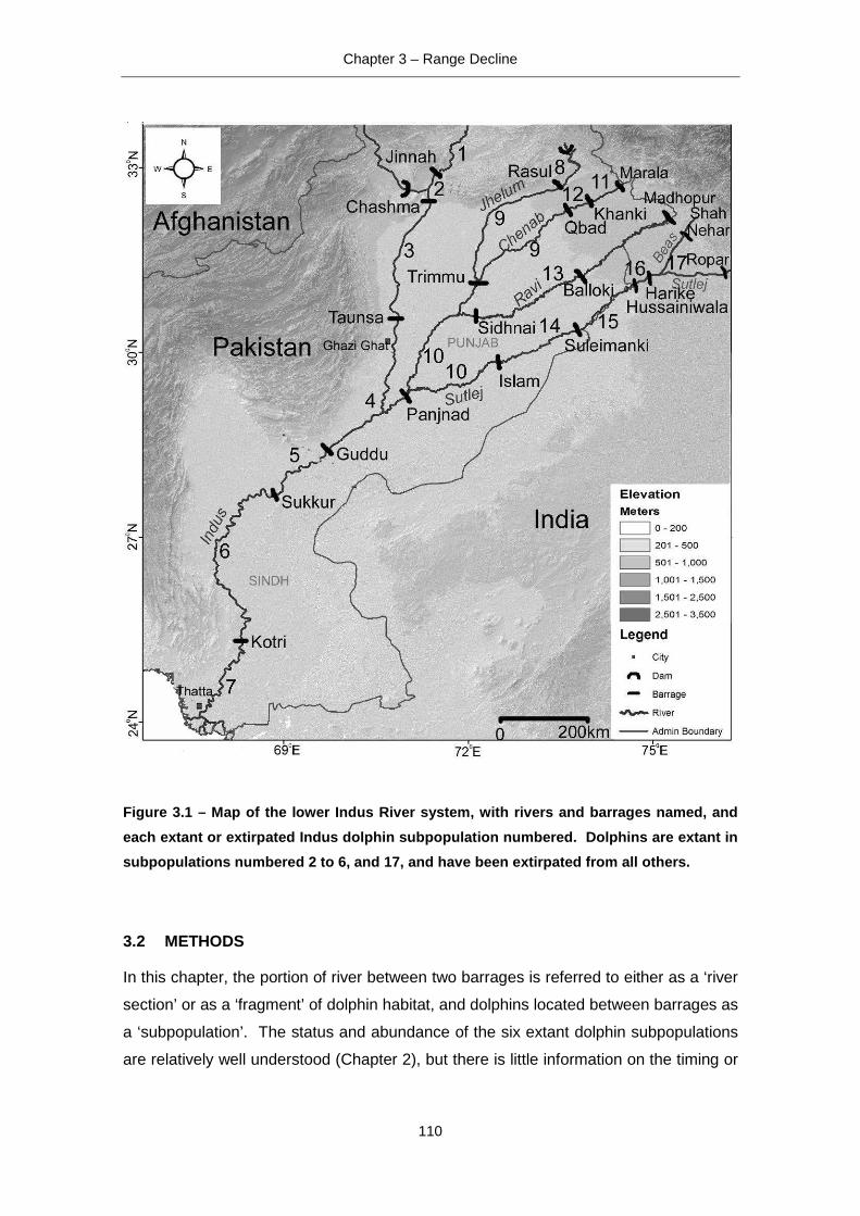
Chapter 3 – Range Decline
110
Figure 3.1 – Map of the lower Indus River system, w ith rivers and barrages named, and
each extant or extirpated Indus dolphin subpopulati on numbered. Dolphins are extant in
subpopulations numbered 2 to 6, and 17, and have be en extirpated from all others.
3.2 METHODS
In this chapter, the portion of river between two barrages is referred to either as a ‘river
section’ or as a ‘fragment’ of dolphin habitat, and dolphins located between barrages as
a ‘subpopulation’. The status and abundance of the six extant dolphin subpopulations
are relatively well understood (Chapter 2), but there is little information on the timing or

Chapter 3 – Range Decline
111
causes of decline from the 11 subpopulations where dolphins are presumed extirpated,
which include nine in the Punjab rivers, and those above and below the current area of
dolphin occupancy between Jinnah and Kotri barrages on the Indus River. This study
consists of two components 1) establishment of a last sighting date of dolphins in each
river section, and 2) generalised linear (GLM) and survival modelling to identify the
principal causes of the dolphin range decline. These are described in Section’s 3.2.1
and 3.2.2 below.
3.2.1 Last Dolphin Sighting Date
Extinction is seldom actually witnessed and it therefore must be inferred (Diamond
1987), however this is complicated by the fact that as animals become increasingly
rare they are much more difficult to detect and their decline more difficult to document.
Dolphins were extirpated from the Punjab rivers in Pakistan during the last century; this
study is especially challenging because the declines occurred a considerable time in
the past. The last sighting dates of dolphins in each river section were established by
a) conducting interviews with elderly fishermen, riverside inhabitants and employees of
the irrigation department, and b) conducting a detailed review of historical literature to
identify dolphin sightings. Due to the great distance between the Punjab rivers and the
Indus delta (approximately 1500km), interviews were not conducted downstream of
Kotri barrage on the Indus River. In addition, the Harike-Hussainiwala section (Fig. 3.1,
subpopulation 16) of the Sutlej River in India was not surveyed because it is a sensitive
international border area. These are the only former dolphin subpopulations for which
no dolphin sighting data were generated.
3.2.1.1 Fishermen Interviews
There are very few sightings of Indus dolphins in the Punjab rivers published in the
scientific literature and, particularly when little scientific background information exists,
local knowledge can provide the only information on historical species distributions.
Local inhabitants often have detailed knowledge about their environments and the
resources on which they depend (Beasley 2007). Interview surveys can provide a cost-
effective way of obtaining information on the basic occurrence and distribution of
species but it is important that the information obtained is carefully verified and
interpreted (Aragones et al. 1997; Tregenza 1992).

Chapter 3 – Range Decline
112
Interview surveys of fishermen and riverside residents along the Jhelum, Chenab, Ravi
and Sutlej Rivers in Pakistan were conducted from 1st to 10th October 2007. The
objectives were to verify the former distribution of the Indus dolphin described by
Anderson (1879) (Fig. 1.4), and to collect reliable dates of dolphin sightings in each
river section. All barrages, headworks, large towns and bridges along the four rivers in
Pakistan were visited by road vehicle. This mode of transportation was selected in
preference to boat because many sections of river had insufficient water to allow vessel
travel. Road access to the river banks is rare, so the use of a vehicle meant that fishers
who reside in riverside villages were targeted. Fishermen who reside on boats (such as
some Mohannas) could not be interviewed. However, given that river flow is severely
depleted, the vast majority of fishers now reside in villages. Interview data from China
regarding the decline of the recently extinct Yangtze River dolphin showed that as soon
as baiji ceased to be encountered on a regular basis they immediately started to be
forgotten by a community (Turvey et al. 2010b). The specific memories of informants
who have encountered a species are unlikely to change significantly (Papworth et al.
2009), but often knowledge is not passed down across generations and over time the
proportion of people in a community who have directly encountered, or remember, the
species decreases (Turvey et al. 2010b). In the Punjab Rivers, dolphins were thought
to have been extirpated between 20 and 80 years ago, depending on the location. To
find informants that had actually witnessed dolphins first-hand our interviews by
necessity targeted elderly people. All interviews were conducted with men, because in
Pakistan, most rural women remain in the home and are less likely than men to have
encountered dolphins.
Interviews must be carefully structured to avoid obtaining misleading results, therefore
care was taken to maximise data quality and address common errors (Gill 1994;
McKelvey et al. 2008). Relatively short (<30 min) closed-question surveys have
generally been recommended for collecting quantifiable or factual information (Moore
et al. 2010). A simple questionnaire was developed consisting of 26 straightforward
questions asked during semi-structured interviews. Interviews were conducted by
myself and local biologists, with individuals in their local language, either Urdu, Punjabi
or Suraiki. Identification cards showing clear photographs and diagnostic features of
the Indus dolphin were shown to participants, along with photos of mugger crocodile
(Crocodilus palustris) and gharial (Gavialis gangeticus) that previously occurred in
Punjab and may be confused with dolphins. Many rural people in Pakistan do not have

Chapter 3 – Range Decline
113
birth certificates and do not know their precise age, so respondent age was recorded in
ten year categories e.g. 60-70 years. A calendar of significant local events was
compiled to assist informants in identifying correct dates (Appendix II). Events that
proved most useful in refining and validating dates were those of the major floods on
each river and the dates of the previous rulers of the country. Attempts were made to
obtain precise dates, but this was not always possible. Where precise dates were not
given, sighting dates were recorded as early, mid or late in each decade.
Questions were focussed on the following topics (see Appendix I for full
questionnaire):
1. Background information: name, age, cast/tribe, number of children/ grand
children (5 questions);
2. Location information: number of years fishing in present location/other
locations (2 questions);
3. Fishing information: gear type, target species, season, and habitat fished (9
questions);
4. General Indus dolphin information (2 questions);
5. Dolphin conservation: causes of decline, causes of mortality (2 questions);
and
6. Dolphin specific sightings: date, location, behaviour, season, number of
individuals (6 questions);
At each new site the fisher community was located, the objective of the survey was
explained to the senior male community member and I requested to interview the
oldest fishermen present.
3.2.1.2 Literature Reviews
A search was conducted through the entire collection of the Journal of the Bombay
Natural History Society (1886-present) and the Journal of the Asiatic Society of Bengal
(1832-1905) for references to river dolphins or porpoises. More recent local resources
such as the Records of the Zoological Survey of Pakistan, Pakistan Journal of
Biological Sciences, Natura (the newsletter of WWF-Pakistan) and the Pakistan
Journal of Zoology were also comprehensively examined. The journal Investigations
on Cetacea, which published many articles about Indus dolphins in the 1970s was also
searched for information on dolphin sighting records in Punjab.

Chapter 3 – Range Decline
114
3.2.1.3 Last Dolphin Sighting Date
The sightings reported in the literature and during interviews were compiled for each
river section, and the most recent taken as the estimated last sighting date. Optimal
linear estimation can be used to identify extinction date based on a sighting record of at
least five sightings (Collen et al. 2010; Solow 1993); however, in this case, there were
an insufficient number of reliable sightings to apply the optimal linear estimation
method and I therefore did not attempt to determine precisely when subpopulations
were extirpated, but instead used the last sighting date as an indicator of when each
subpopulation disappeared (Butchart et al. 2006). Recognising that it is difficult to
precisely date extirpation, the spatial and temporal analysis, described below, was
conducted by assigning inexact sighting dates to 5 year intervals (Butchart et al. 2006).
If the last sighting date was, for example, early in the 1970s, for the purposes of this
investigation a date of 1972 was assigned, if it was mid 1970s, 1975 was assigned,
and if it was late 1970s the date used was 1978.
3.2.2 Identifying the Causes of Range Decline
3.2.2.1 Data Set
There have been 33 river sections of different lengths created since the onset of
barrage construction, comprising 16 larger former fragments and 17 smaller current
fragments (Appendix III). For example, a section of the Indus River was isolated
between Jinnah and Sukkur barrages in 1946; this 693 km river section existed for 13
years until it was split into two parts (403 & 190 km in length) on completion of Taunsa
barrage in 1959. The historical progression of habitat fragmentation has obviously
played a role in the spatial and temporal pattern of Indus dolphin range decline.
However, the interview data show that dolphins were present in all 16 former habitat
fragments from the date of their creation until they were superseded by new smaller
fragments. The extirpation of Indus dolphins occurred exclusively within the 17 river
sections that are present today and that have existed in their present configuration for
approximately 50 years. For this reason, and because historical environmental data are
lacking, it is appropriate to focus the following analysis of the causes of Indus dolphin
range decline exclusively on the 17 current sections of the Indus dolphin’s former
range.

Chapter 3 – Range Decline
115
3.2.2.2 Potential Drivers of Range Decline
The following seven explanatory variables that may have contributed to the Indus
dolphin range decline were determined for all 17 current river sections.
1. Fragmentation date- The year that each of the current dolphin subpopulations was
created was assigned as the date that the second of the two bounding barrages
became operational. For the dolphin subpopulation upstream of Harike barrage in
India the isolation date was assigned as the completion date of Hussainiwala
barrage which is located only 30km downstream of Harike, and was completed 28
years earlier, isolating dolphins upstream.
2. River length - The number of river kilometres between two barrages.
3. Proximity to range edge – Satellite images projected in ArcView 3.2 were used to
determine the proximity of each river section from the historical distribution limit
recorded by Anderson (1879). This was determined by measuring the distance
along the river’s course from the former range limit to the barrage located closest
to the range core. The barrage closest to the range core was selected because
dolphin habitat was assumed to improve closer to the range core and that dolphins
may persist at this end of a subpopulation. This variable accounts for increasing
extinction risk at the periphery of the subspecies range.
4. Size of river - The mean annual discharge in Million Acre Feet (MAF) reported for
each river prior to implementation of the Indus Water Treaty (IUCN 2011). This
single figure does not account for changes in discharge along the course of a river,
or over time, but provides an indicator of comparative river size.
5. Confluences - River dolphins are patchily distributed in the Indus River, and occur
with higher frequency at confluences (Chapter 4). Hotspots of Ganges dolphin
distribution also occur at the confluence of tributaries with the Ganges mainstem
(Sinha et al. 2011; Sinha et al. 2010). The number of river confluences within each
subpopulation was included as an indicator of the presence of favourable habitat.
6. River slope – The elevation of each barrage was obtained from a digital elevation
model of Pakistan and India, and the average slope within each river section was
calculated as the drop in elevation between the up and downstream barrages, or
upstream range limit in the case of peripheral segments, divided by the length of

Chapter 3 – Range Decline
116
river. Slope exerts a direct effect on flow velocity and sediment transport and
therefore influences dolphin habitat.
7. Dry season river discharge – River discharge data were obtained for all twelve
barrages and two dams north of Guddu on the Indus River system in Pakistan for
the period July 2008 to October 2011 (3 ¼ years). The daily discharge below
Guddu and Kotri barrages were obtained from October 2010 to October 2011 (~1
year), and discharge below Sukkur barrage was obtained from April 1994 to
January 2000, and October 2010 to October 2011 (6 ¾ years). For each dolphin
subpopulation two discharges were available: a) discharge released from the
upstream barrage, and b) the discharge received at the downstream barrage. As
almost no water is extracted between barrages (it is extracted at barrages), these
figures were almost identical, and therefore only discharge from the upstream
barrage was used in the models. Discharge was often not recorded on Sundays or
holidays, so the missing data were interpolated. It is very low flows that are likely to
adversely impact dolphins, and as the average discharge was heavily influenced
by occasional flood pulses, the median daily discharge during the dry season (1st
October to 31st March) was determined using only years for which there was an
entire dry season’s data. Discharge of Indus tributaries in India is classified
information and could not be obtained, therefore discharge above and below
Harike barrage was estimated from historical published flows, by examining
satellite images and aerial photos of the river at different times of year, and from
information on the diversion capacity of canals. The number of years of data
available differed according to barrage but the temporal discharge pattern was
predictable and similar across years in each location. There were however large
differences in discharge among different barrages in the Indus system (ANOVA,
F=1658.9. df=14, p=<0.0001).
3.2.2.3 Modelling Causes of Range Decline
To explain, and attempt to identify the causes of the spatial and temporal pattern in
Indus dolphin subpopulation extirpation, GLMs and a survival analysis were used with
the seven explanatory variables described above as predictors of continued presence
of river dolphins. Generalised Additive Models (GAMs) were used in the initial data
exploration to visually investigate whether the relationship between the predictor and
explanatory variables was linear and if not which type of transformation could be used

Chapter 3 – Range Decline
117
to best account for non-linearity (Redfern et al. 2006). Three sets of models were
developed, with objectives summarised below:
Models of the spatial pattern of dolphin persistence: The objective of the first set of
models was to identify which factors best explained the observed geographic pattern of
range decline and dolphin presence. All putative Indus dolphin subpopulations (except
for Harike-Hussainiwala that has not been surveyed for dolphins) (n=16) were included.
The presence or absence of a dolphin population was modelled using a binomial error
distribution, with presently extant populations coded as 1 and extirpated populations
coded as 0. The best fitting models were then used to predict the probability that
dolphins are still present in the Harike-Hussainiwala subpopulation.
Models of the temporal pattern of decline: The objective of the second model set was
to identify which factors were most strongly related to when subpopulations were
extirpated. Only those dolphin subpopulations that have already been extirpated and
for which there was a last dolphin sighting date (n=9) were included. The number of
years before the present date (PD=2011) of the last dolphin sighting (PD-LDS) was the
response variable. As the response variable was a count of years that was over-
dispersed relative to the Poisson distribution, the data were modelled using a GLM with
a quasi-Poisson error distribution.
Models of time to extirpation: The third model set was designed to investigate which
factors influenced the speed with which subpopulations were extirpated following their
isolation between barrages. The time to extirpation was calculated as the number of
years that elapsed from the isolation date to the last dolphin sighting date. The time to
extirpation only for subpopulations already extirpated could have been modelled fairly
simply using a GLM with Gamma errors, however, subpopulations that are still extant
also have information to contribute to understanding the speed of extirpation. To allow
inclusion of this additional information, extant subpopulations were also included in a
survival regression model, which is specifically designed to model time to death or time
to failure data and allows for censoring (Crawley 2007). The last sighting date for
subpopulations that are still extant was calculated by subtracting the isolation date from
the last sighting date assigned as the current year, 2011. Thirteen subpopulations
(subpopulations 2, 10, 12 and 16 were excluded because of missing data), were
included in the model, and each was qualified with a status assignment, where
1=extirpated, and 0=extant. Time to extirpation and status form the Kaplan–Meier
survivorship object, which was the predictor variable modelled using the survreg

Chapter 3 – Range Decline
118
function in the survival library of the programme R (R Development Core Team 2010).
Both an exponential error distribution associated with a constant risk of extirpation
following isolation, and a Weibull error distribution, that fits data where the risk of
extirpation rises with subpopulation age, were fitted to the data (Crawley 2007). The
Weibull distribution was selected as it provided a significantly better fit (ANOVA, p=0.01
and delta AIC 5.447).
All models were implemented using the programme R 2.12.1 (R Development Core
Team 2010). The datasets were small, 16 subpopulations in the binomial models, 9 for
the last sighting date models, and 13 for the time to extirpation models, so considering
the rule-of-thumb suggested by Crawley (2007) the number of parameters estimated
was constrained to no more than one third of the total data points. Logit, probit and
cloglog link functions were included in global models and the logit function which
resulted in the best fit applied. Variance Inflation Factors (VIFs) that demonstrate the
degree of collinearity between variables were generated from the maximal models and
collinear variables removed until variance inflation factor scores were less than five
(Crawley 2005; Zuur et al. 2009). Retaining collinear variables can inflate sampling
variances and create unstable parameter estimates potentially affecting which
variables are retained in final models (Crawley 2005). Three two-way interactions that
described potentially meaningful relationships between variables (isolation date and dry
season discharge, isolation date and river length, and river length and proximity to
range edge) were included in model sets, as well as second and third order
polynomials of significant variables. The binomial and survival models were simplified
using backwards stepwise selection based on Akaike’s Information Criteria (AIC)
(Akaike 1973). Quasi-Poisson models were selected on the basis of quasi-AIC (QAIC)
scores that incorporated the dispersion parameter from the full model, and non-
significant terms were sequentially dropped based on their levels of significance.
Models separated by at least two AIC/QAIC points were assumed to be significantly
different (Burnham and Anderson 2002). If removal of a variable resulted in an increase
in AIC of two points or more it was returned to the candidate models because it
contributed important information. Goodness of fit for the GLMs was measured by
determining the proportion of the total deviance explained by the final model, and by
each of the significant explanatory variables. Model plots were examined for non-
normality of errors, heteroscedasticity and influential points (Crawley 2007; Fox 2008).

Chapter 3 – Range Decline
119
3.3 RESULTS
3.3.1 Interview Surveys
A total of 57 interviews were conducted: 23 on the Chenab River, 11 on the Jhelum,
9 on the Ravi, 9 on the Sutlej, and 5 on the Indus above Jinnah barrage. Fishermen
interviewed ranged in age from 30 to more than 90 years, however most respondents
were aged between 50 and 60 (13 individuals), 40 to 50 years (12 individuals), and
70 to 80 years (10 individuals). Our focus on retired fishermen, and on areas from
which dolphins have already been extirpated meant that the communities were forth-
coming with information because it was not regarded by them as sensitive. However,
there were very few elderly members of each fishing community and our pool of
available informants was consequently small.
The majority of fishing communities interviewed on the rivers in Punjab were from the
Jebail, Malah or Mohanna tribes and had been involved in fishing for many
generations. These fishing communities are one of the poorer sections of society in
an already impoverished region. The fishing tribes are closely related and some
claim to have moved from Sindh several generations ago. Members of some of these
communities may have been involved in dolphin hunting in the past, but there is no
evidence that this practice continues today. On the Jhelum and Chenab most
fishermen spoke Punjabi but near Panjnad and on the Sutlej Suraiki was the
predominant local language. The name of the Indus dolphin in both languages is
bhulan which is reminiscent of the sound dolphins make as they take a breath.
Of the people interviewed, 79% were full-time commercial fishermen or fish
contractors and the remainder were part-time fishermen who fished for subsistence
or recreation. Of those who specified, all fished in the rivers, although a few also
fished in the lakes adjacent to barrages and in canals. All fishermen agreed that
June to August (the flood season) is the spawning season for most river fish and that
fishing is banned by the Government for those three months. 100% of fishermen
reported that there were less fish than in the past, and this was due to either reduced
flows and/or pollution. 82.7% of informants had heard of Indus dolphins and 65.4%
reported that they, or a close family member, had seen one. Many were familiar with
dolphins from sightings on the Indus River at Taunsa barrage or in Sindh but were
much less likely to have seen dolphins in the Punjab Rivers. Young informants,

Chapter 3 – Range Decline
120
especially those under the age of 40, were less likely to have encountered dolphins
than older individuals (Fig. 3.2).
Figure 3.2 – Proportion of respondents that had see n Indus dolphins according to age
group
3.3.2 Last Dolphin Sighting Date
The interview surveys did not generate any evidence that dolphins persist even in small
numbers in any of the Punjab rivers in Pakistan. The following is a description of the
historical Indus dolphin sightings, compiled from interviews and literature; these are
also compiled in Table 3.1.
3.3.2.1 Jhelum River
Only 18% of informants (2 of 11) could recall dolphins in the Jhelum River. Dolphins
were reported to have been present near to Rasul barrage in the mid-1960s by one
informant and in the mid-1950s by a second. Reeves et al. (1991) reported that
dolphins were in the Jhelum River in the 1970s. Fishermen reported seeing dolphins
near Jhelum town, upstream of Rasul barrage, in 1975 but these animals were
subsequently noted to have disappeared after the major flood the following year (Pilleri

Chapter 3 – Range Decline
121
and Bhatti 1978). A dolphin sighting in the Jhelum River prior to the floods in 1976
(Arain 1978) was cited by Reeves et al. (1991).
3.3.2.2 Chenab River
There are no records of dolphins near Khanki or Qadirabad barrages on the Chenab
River since Anderson created his map in 1879. The oldest fishermen interviewed
recalled seeing a group of dolphins at the Jhelum-Chenab confluence in the 1930s as
he was swimming across the river. At Panjnad barrage, virtually all people interviewed
had seen dolphins downstream of the barrage during the summer when dolphins move
upstream from the Indus. Above Panjnad barrage in the Chenab River, fishermen
reported that dolphins were present in the 1940s prior to the partition of India. There
was a sighting in the 1950s in the Chenab River near to Muzaffaragarh (approximately
80km upstream of Panjnad barrage), sightings in the early 1970s between Panjnad and
Trimmu barrages were reported by Roberts (1997) and a sighting just downstream of
Trimmu barrage in 1981 was documented (Reeves et al. 1991). No dolphins were
recorded in the Chenab in the winter of 1963/64 (Taber et al. 1967) and Khan and Niazi
(1989) suggested that the Chenab dolphin population had disappeared in the 1970s.
3.3.2.3 Ravi River
The only record of dolphins in the Ravi River, was one person who reported sighting
dolphins from Sidhnai Barrage in the early 1960s. There were no dolphin records from
upstream of Balloki barrage, which concurs with the upstream dolphin distribution limit
of Lahore depicted by Anderson (1879).
3.3.2.4 Sutlej River
In contrast to interviews conducted on the other Punjab rivers, all respondents could
recall dolphins being present in the Sutlej River. In the winter of 1977-78 three dolphins
were reported in the Sutlej River below the Islam headworks (Pelletier and Pelletier
1980). They were reported to be present above Islam barrage until 1966 by two
informants, present until the mid-1960s by another and the early 1970s by a fourth.
Upstream of Suleimanki barrage all informants, and also some that were resident on
other Punjab rivers, reported that dolphins were reliably present until the late 1980s.
Two informants said that the dolphin population above the barrage disappeared in
1985, and another two thought that the population was wiped out by the large flood in

Chapter 3 – Range Decline
122
1988. In 1989, Khan and Niazi (1989) noted that the area upstream of Suleimanki
barrage had supported dolphins until recently. T.J. Roberts reported that dolphins were
present upstream of Suleimanki in 1972 (Roberts 1977), and subsequently that they
were still present in the 1980s (Roberts 1997). Dolphins were also reported upstream
of Suleimanki barrage in 1989 by experienced biologist Z.B. Mirza (pers. comm.).
Irrigation department employees at Suleimanki barrage believed that dolphins were
extirpated from the Sutlej because the Balloki-Suleimanki link canal was bringing
extremely polluted water from the Ravi River to the Sutlej.
Table 3.1 - Indus dolphin sighting records in the P unjab rivers since the 1920s.
Subpopulations numbers refer to those depicted in F ig. 3.1 and 3.3.
River Subpopulation # Sighting Date Source
Indus 1. Upstream Jinnah 1.
2.
Kalabagh: mid
1950s
Kalabagh: 1950s
Fisher interview, this study
Fisher interview, this study
Jhelum 8. Upstream Rasul 1. 1975 (Pilleri and Bhatti 1978)
Jhelum-
Chenab
9. Trimmu-Rasul-
Qadirabad
1.
2.
3.
4.
5.
Jhelum: Mid-1960s
Jhelum: Mid-1950s
Confluence: 1930s
Jhelum: 1970s
Jhelum: 1976
Fisher interview, this study
Fisher interview, this study
Fisher interview, this study
Reeves et al. (1991)
(Arain 1978)
Chenab 11. Khanki-Marala - No sightings -
Chenab 12. Qadirabad-Khanki - No sightings -
Chenab-
Sutlej-Ravi
10. Panjnad-Islam-
Sidhnai-Trimmu
1.
2.
3.
4.
5.
1950s
1940s
1981
Early-1970s
Winter 1977-78
Fisher interview, this study
Fisher interview, this study
(Reeves et al. 1991).
(Roberts 1997)
(Pelletier and Pelletier
1980)
Ravi 13. Sidhnai-Balloki 1. Early-1960s Fisher interview, this study
Sutlej-Beas 17. Harike-Ropar-
ShahNehar
1. Extant (Behera et al. 2008)
Sutlej 16. Hussainiwala-
Harike
- Un-surveyed -
Sutlej 15. Suleimanki-
Hussainiwala
1.
2.
1988
1988
Fisher Interview, this study
Fisher Interview, this study
Chapter 3 – Range Decline
123
3.
4.
5.
6.
7.
8.
1985
1985
1989
1972
1980s
1980s
Fisher Interview, this study
Fisher Interview, this study
Z.B. Mirza, pers. comm.
(Roberts 1977)
(Khan and Niazi 1989)
(Roberts 1997)
Sutlej 14. Islam-Suleimanki 1.
2.
3.
4.
1966
1966
Mid-1960s
Early-1970s
Fisher interview, this study
Fisher interview, this study
Fisher interview, this study
Fisher interview, this study
3.3.3 Dynamics of Range Decline
Fig. 3.3 illustrates the approximate last dolphin sighting date in each subpopulation,
visually demonstrating the spatial and temporal pattern of Indus dolphin range decline
in the Punjab rivers. The memories of informants were less exact as sighting dates
were further in the past. There are also fewer sightings records for subpopulations that
were extirpated longer ago. Despite this, the data should still indicate the general
pattern. Records indicate that dolphins were extirpated first from the upper Chenab
River, then from above Jinnah barrage on the Indus, the Ravi River, the Jhelum, and
finally the Sutlej. The last subpopulations to disappear were those upstream of Panjnad
barrage and upstream of Suleimanki barrage, both of which persisted until the 1980s.
In some rivers upstream populations were extirpated prior to those downstream, but
this pattern is disrupted by the continued presence of dolphins at the upstream
periphery of their former range in the Beas River in India.

Chapter 3 – Range Decline
124
Figure 3.3 - Spatial and temporal dynamics of the I ndus dolphin range decline. Numbers
refer to dolphin subpopulations listed in Table 3.1 & Fig. 3.1. Grey boxes indicate
barrages.
3.3.4 Causes of Range Decline
Of 17 sections of river, dolphins are extant in six, are presumed extirpated from ten,
and in one dolphin presence or absence is unknown. Each Indus dolphin
subpopulation, its status, estimated last dolphin sighting date, and physical
characteristics are listed in Table 3.2. These data were included in each of the range
decline models described below. Subpopulations 11 and 12, on the upper Chenab
River were presumably extirpated first, the last sighting date is that reported by
Anderson (1879). Due to the lack of reliable sighting data time to extirpation was not
calculated for these two subpopulations.

Chapter 3 – Range Decline
125
Table 3.2 – Details of extant and extirpated Indus dolphin subpopulations
# Subpopulation River Date a
Isolated
Extant (1)
Extirpated (0)
Last
Sighting
Dateb
Time to c
Extirpation
Length
(km) d
River
Sizee Conf f
Median g
Discharge
Dist
(km) h
Slope
m/km
13 Balloki-Sidhnai Ravi 1886 0 1962 74 175 7 0 0 175 0.29
11 Marala-Khanki Chenab 1892 0 1879 N/K 35 26 0 4140 0 0.54
8 Upstream Rasul Jhelum 1901 0 1975 74 50 23 0 27000 71 0.72
15 Hussainiwala-Suleimanki Sutlej 1926 0 1988 62 110 14 0 7000 287 0.18
14 Suleimanki-Islam Sutlej 1927 0 1972 43 145 14 0 0 438 0.26
17 Ropar,ShahNehar-Harike Sutlej-Beas 1927i 1 N/A N/A 220 14 1 15000k 148 0.38
10 Islam,Sidhnai,Trimmu-
Panjnad
Chenab, Sutlej,
Ravi 1933
0 1981 48 435
26 2 1231 610
0.11
9 Rasul,Qadirabad-Trimmu Chenab, Jhelum 1939 0 1975 36 490 26 1 6975 327 0.13
1 Upstream Jinnah Indus 1946 0 1955 9 35 93 0 40000 35 0.89
16 Harike-Hussainiwala Sutlej 1955 N/K N/K N/K 30 14 0 5000k 184 0.33
6 Sukkur-Kotri Indus 1955 1 N/A N/A 318 93 0 6400 520 0.09
7 Downstream Kotri Indus 1955 0 N/K N/K 222 93 0 3922 205 0.09
3 Chashma-Taunsa Indus 1959 1 N/A N/A 230 93 0 43000 351 0.23
4 Taunsa-Guddu Indus 1962 1 N/A N/A 277 93 1 37262 636 0.21
5 Guddu-Sukkur Indus 1962 1 N/A N/A 126 93 0 34916 645 0.17
12 Khanki-Qadirabad Chenab 1967 0 1879 N/K 45 26 0 578 0 0.44
2 Jinnah-Chashma Indus 1971 1 N/A N/A 60 93 0 47127 122 0.45
# Dolphin subpopulation number, also shown in Fig 3.1 and 3.3 and Table 3.1, a Date that dolphins were confined between two barrages, taken as the completion date of the downstream barrage, b Where sighting dates were imprecise they were rounded, for example to 1972, 1975 or 1978. C The time that elapsed from the isolation date to the last sighting date d Length of river between barrages e Annual average flows calculated by averaging daily flows for the period 1922 to 1961 (IUCN 2011). f Number of river confluences occurring within subpopulation g Median daily discharge between October 1st and March 31st (the dry season) from the upstream barrage in cubic feet per second. hDistance to former range limit described by Anderson (1879)(Fig. 1.2). i Harike isolation date taken from completion date of Hussainiwala barrage nearby. k Estimated. N/K = not known. N/A = not applicable

Chapter 3 – Range Decline
126
3.3.4.1 Causes of the Spatial Pattern of Indus dolphin Range Decline
Where dolphins are still extant the mean dry season river discharge was 30,618 cusecs
(SD=16,241) compared to a mean of 9,044 cusecs (SD=13,489) in locations from
which they have been extirpated. Characteristics of river sections where dolphin
subpopulations are extant or extirpated were compared using t-tests. After Holm
correction for 6 tests no results were significant, although for subpopulations that are
still extant mean river size (t-test, t=2.731, df=10.4, p=0.08) and median dry season
discharge (t-test, t=2.736, df=9.1, p=0.08) were greater, and mean date of
subpopulation isolation later (t-test, t=2.739, df=14.0, p=0.08) (Fig. 3.4). In general,
sections of river where dolphins are still present were fragmented by barrages later, are
further from the range periphery, are of larger size, have a shallower slope and have
greater dry season discharge than river sections where dolphins are no longer found.
Figure 3.4 –Characteristics of river sections where river dolphins are present and where
they have been extirpated.

Chapter 3 – Range Decline
127
16 subpopulations, six where dolphins are extant and ten where they have been
extirpated were included in GLMs for binary data. Explanatory variables were not
significantly correlated (Spearman’s rank correlation test) however, the variance
inflation factors generated from the full model indicated that river discharge and slope
were collinear. Slope was considered to be less important than discharge in explaining
dolphin distribution and range decline and was therefore removed from further
candidate models. No interactions or polynomials were retained. The final model which
best explained the observed spatial pattern in Indus dolphin range decline retained the
explanatory variables ‘distance from range edge’ and ‘dry season river discharge’. The
probability that an Indus dolphin subpopulation is still extant increases with increasing
distance from the range edge, and with increasing dry season river discharge (Fig. 3.5;
Table 3.3).
Table 3.3 – Summary of spatial range decline model output
Model AIC ∆
AIC
%
explained
Deviance
n
Deviance
Q Range Is. Date L Conf Size
1 17.26 - 46.8 2 7.13 2.77 - - - -
2 18.39 1.67 50.9 3 7.13 2.77 0.87 - - -
3 20.26 3.00 51.5 4 7.13 2.77 0.79 0.21 - -
4 22.24 4.98 51.6 5 7.13 2.77 0.51 0.49 0.03 -
5 23.92 6.66 53.1 6 7.13 2.77 0.82 0.49 0.03 0.002
n = number of parameters, Is. Date = Isolation Date, L=Length of river section, Range =
Distance from range edge, Size = River size, Conf. = confluences, Q=River discharge. Model in
bold was the final selected model.
The best fitting model was used to predict the probability that dolphins are still extant in
the Harike-Hussainiwala river section in India that has not been surveyed for dolphins.
The probability that dolphins are still present was predicted to be only 5.2%. This is not
unexpected given that this section has very low winter discharge and is near the
periphery of the dolphin’s range, both factors that increase the likelihood of
subpopulation extirpation.

Chapter 3 – Range Decline
128
Figure 3.5 – Probability that an Indus dolphin subp opulation is extant according to
proximity to the edge of the former range and the m edian dry season discharge (cubic
feet per second).
3.3.4.2 Causes of the Temporal Pattern of Indus Dolphin Range Decline
Only those subpopulations that have already been extirpated, and for which there was
a reliable last sighting date, were included in this component of the analysis (n=9).
Spearman’s rank correlations of the last dolphin sighting date and each of the potential
drivers of decline showed no significant relationships except between last sighting date
and distance from the former range edge (Spearman’s rank, S=206.1, p=0.030). The
final model with the lowest QAIC retained distance from former range limit, dry season
discharge and river size as the three variables that best describe the temporal pattern
of Indus dolphin subpopulation extirpation (Table 3.4). No interactions between
variables or polynomials were retained in the final models. The relationship between
discharge and last sighting date was negative indicating that dolphin subpopulations
were extirpated earlier in locations where dry season discharge was lower. Earlier
extirpation also occurred in subpopulations located near the periphery of the
subspecies range (Fig. 3.6). River size was not strongly significant and explained a

Chapter 3 – Range Decline
129
very small proportion of deviance but removing it from the final model increased the
AIC by 6 points and it was therefore retained.
Table 3.4 – Summary of temporal range decline model outputs
Model AIC ∆
AIC
%
explained
Deviance
n
Deviance
Q Range Is. Date L Conf Size
1 29.44 78.6 2 39.7 123.3 - - - -
2 24.68 93.1 3 66.9 123.3 - - - 3.1
3 26.40 93.8 4 60.1 123.3 3.8 - - 7.5
4 28.25 94.1 5 60.1 123.3 3.8 - 0.7 7.5
5 31.58 95.5 6 60.1 123.3 3.8 0.4 3.2 7.5
n = number of parameters, Is. Date = Isolation Date, L=Length of river section, Range =
Distance from range edge, Size = River size, Conf. = confluences, Q=River discharge. Model in
bold was the final selected model.
Figure 3.6 – Relationship between the number of yea rs since a dolphin was sighted and
a) subpopulation distance from historical range edg e, and b) median dry season
discharge, the two significant explanatory variable s retained in quasi-Poisson GLM
models of the temporal pattern of Indus dolphin ran ge decline.

Chapter 3 – Range Decline
130
The best fitting model was then used to predict the last sighting date for subpopulations
that are still extant. Results were as expected, with very recent (0-20 years before
present) sighting dates generated for all extant subpopulations. The only anomalous
result was for the subpopulation between Sukkur and Kotri barrages (subpopulation 5)
(Fig. 2.1) on the Indus River. Recent surveys indicate that dolphins are present in small
numbers in this river section (Chapter 2), but the model predicted that dolphins were
extirpated 91 years (SE=43) ago from this river section.
3.3.4.3 Time to Subpopulation Extirpation
The mean time from subpopulation creation to dolphin extirpation was 49 years
(SD=23, range=9-74), and for populations that are still extant, the mean time from
subpopulation isolation to present was 55 years (SD=15, range=40-84). The slope
parameter was included in this model set, and the final survival model retained three
variables: median dry season river discharge (p=0.043), isolation date (p=0.054) and
slope (p=0.040). Following isolation between barrages a dolphin subpopulation was
extirpated more quickly as dry season river discharge decreased. Subpopulations
persisted longer where the river slope is more gentle (e.g. in the lower reaches) and
those created earliest persisted for longer than those in more recently subdivided river
sections. The subpopulation survival curve (Fig. 3.7) indicates that after 50 years of
isolation there is a less than a 50% chance that an Indus dolphin subpopulation will still
be extant, and after 100 years this probability dropped to 38%. Of the six
subpopulations that are still extant, the model fit the shortest time to extirpation for the
subpopulation upstream of Harike headworks, and that between Sukkur-Kotri barrages
(65 and 64 years, respectively), and the longest time to extirpation for the Chashma-
Taunsa, Taunsa-Guddu and Guddu-Sukkur subpopulations (463, 305 and 309 years,
respectively).

Chapter 3 – Range Decline
131
Figure 3.7 – Probability that an Indus dolphin subp opulation is extant with increasing
time of isolation
3.4 DISCUSSION
3.4.1 Dynamics of Range Decline
Care must be taken when evaluating anecdotal evidence on the occurrence of rare
species. There are cases where anecdotal evidence has led to vast overestimations of
endangered species range and abundance (McKelvey et al. 2008) and also, where
locals were unaware that a rare species occurred nearby (Hajjar 2011). The former
distribution of dolphins indicated by interviews in this study concurs closely with the
distribution recorded by Anderson in 1879. The only ambiguous area was the upper
reaches of the Chenab River, where dolphins were reported to be present in the 1870s
but interviews generated no records. It may be that the map of Anderson was
inaccurate and that dolphins were never regularly present in those areas or that
dolphins disappeared from the upper Chenab so long ago that they are no longer
remembered by local inhabitants. As a species becomes rarer the number of false
positive sightings is likely to increase. However, despite the rarity (or absence) of

Chapter 3 – Range Decline
132
Indus dolphins in the Punjab rivers, our interview data resulted in no positive recent
sighting records. Species that have not been recorded for decades are more likely to
have become extinct because of the length of time without positive sightings (Butchart
et al. 2006). Butchart et al. (2006) defined ‘possibly extinct’ species as those species
with recent records where:
1. The decline has been well documented;
2. Severe threatening processes are known to have occurred (e.g. extensive
habitat modification);
3. The species possess attributes known to predispose taxa to extinction; and
4. Recent surveys have been adequate but have failed to detect the species.
The data collected from the 10 river sections with no recent dolphin sightings meet all
of the above criteria, and I therefore conclude that there is sufficient evidence to
assume that Indus dolphins have been extirpated from the Jhelum, Chenab, Ravi and
Sutlej Rivers in Pakistan, as well as upstream of Jinnah Barrage and downstream of
Kotri barrages. Indus dolphins remain in only six sections of river (five on the Indus
and one on the Beas) bounded by irrigation barrages.
The spatial pattern of Indus River dolphin decline is very different from the gradual
decline in abundance described for the Yangtze River dolphin (Turvey et al. 2010a).
Indus dolphin range decline has been dictated by the contagion-like spread of
extinction factors, in this case water extraction. Dolphins continue to persist in the
range core primarily because the greatest threats are concentrated in the periphery of
the subspecies range (Lomolino and Channell 1995).
The persistence of dolphins in the Beas River, upstream of Harike Barrage in India is
likely to be due to the presence of constant water supplies that have been little
depleted by diversions (Behera et al. 2008). This demonstrates that in the presence of
sufficient water, and an absence of other threats, river dolphins can persist for decades
even in relatively small fragments of habitat. Dolphins in the Beas River occur in what
is effectively an island as the river downstream is virtually dry, and there is only
connectivity with the rest of the river system for a few weeks each year during the
monsoon floods. This subpopulation is of high conservation importance, as all other
dolphin subpopulations occur in a single river and are therefore at risk of extirpation
from environmentally correlated catastrophes (Gilpin 1990; Reed 2004; Soulé and
Simberloff 1986).

Chapter 3 – Range Decline
133
3.4.2 Causes of Range Decline
3.4.2.1 Water Extraction
The river discharge data used in these models were from approximately the last ten
years but they explained well the pattern of dolphin decline that occurred decades ago.
There is an implicit assumption that present patterns of discharge reflect those in the
past. Although discharge fluctuates annually, and has generally declined, the relative
discharge among barrages (e.g. the spatial relationship) has remained relatively
constant with the same locations consistently reporting high (e.g. the upper Indus) and
low discharge (e.g. Punjab Rivers and downstream Sukkur) now and in the past.
The clear result of this study was the relationship between low dry season river
discharge and the decline of the Indus dolphin. Reduced flows directly impact dolphins
by reducing the physical space available to them, reducing average water velocity and
depth and increasing water temperatures. Large-scale water extraction has rendered
some tributaries of the Indus River trickles in many places and in these conditions, river
dolphins cannot persist. It is obvious that if rivers become dry, species such as river
dolphins, that rely entirely on freshwater will be extirpated. It is probable that if
discharge falls to zero for a short period of time (e.g. 1 day) that some dolphins will be
able to survive in pools until higher flows return. Consecutive days of zero flow, greater
than the flow lag time between barrages (approximately 5-10 days depending on
section), would render an entire river section virtually dry and quickly extirpate resident
dolphins as well as other aquatic life. It is unclear whether it is the long-term reduced
flows, or a period of zero flows, that extirpated dolphins from the Punjab rivers.
However, it is certain that the flow required to maintain sufficient suitable habitat for a
healthy population of dolphins is considerably greater than zero.
Reduced flow also impacts river dolphins through numerous indirect mechanisms, as
the flow regime is a key driver of the ecology of rivers. It determines river habitat, and
habitat in turn influences the distribution and abundance of aquatic organisms (Bunn
and Arthington 2002; Nilsson et al. 2005). Flow regulation and water diversion results
in declines in fish diversity, the dominance of generalist fish species, and increased
success of invasive species (Bunn and Arthington 2002; Copp 1990; Gehrke et al.
1995; Pusey et al. 1993). All these factors are likely to have adversely affected Indus
dolphins.

Chapter 3 – Range Decline
134
Dams and diversions typically dampen flood peaks, reducing the frequency, extent and
duration of floodplain inundation that determines how long fish can gain access to
nursery habitat and food. Reduced discharge has almost certainly affected recruitment
of many Indus River species, and may have resulted in declines in dolphin prey. Floods
are also important spawning cues for fish, benthic microorganisms, phytoplankton,
zooplankton and possibly also Indus dolphins (Bunn and Arthington 2002). In the past
Indus dolphins were reported to shift their distribution in response to the annual flood
(Anderson 1879), but these movements are now blocked by irrigation barrages. Given
the predictable annual flood that initiates spawning for many fish species, it seems
likely that dolphin calving is also seasonal, in which case habitat fragmentation and
water extraction may have negative impacts on dolphin recruitment. Water extraction
contributes to, or interacts with, numerous other factors that may have played a role in
the decline of Indus dolphins, including increased water temperature, higher
concentrations of nutrients and pollutants, and an increase in exotic species (Allan and
Flecker 1993; Xenopoulos and Lodge 2006).
3.4.2.2 Fragmentation
Interestingly, the date of habitat fragmentation was not selected by models as a
significant factor driving the dolphin’s decline, however, depleted river discharge and
fragmentation by barrages are inextricably intertwined as barrages are responsible for
water extraction, and they are a physical barrier that prevents the dispersal of dolphins
out of impacted river reaches (Nilsson et al. 2005). Desert fish in fragmented habitats
were more than five times as likely to have suffered local extirpations than similar
species with more continuous habitat, and fragmentation of the Indus dolphin habitat
has undoubtedly been the major factor involved in its decline (Fagan et al. 2002).
Habitat fragmentation will also reduce the resilience of river dolphins to future threats,
such as climate change. In free-flowing rivers, many organisms are likely to adapt to
climate change by concomitant shifts in distribution; however, in fragmented and
regulated rivers, dispersal is strongly limited thereby exacerbating the future impacts of
climate change on them (Nilsson et al. 2005).

Chapter 3 – Range Decline
135
3.4.2.3 Small Populations
The decline of Indus dolphin subpopulations at the range periphery prior to those at the
core generally supports the theory that where animals are least abundant they are
likely to be extirpated first (Nilsson et al. 2005). Although it is water extraction
combined with habitat fragmentation that have driven the decline of the dolphin, these
factors generally resulted in the earlier and more rapid extirpation of the smaller
populations at the range periphery. It is important to note, however, that the factors that
reduce a species range are frequently quite different from those that eliminate the last
individuals (Burbidge and McKenzie 1989). The factors identified above may be
reducing the Indus dolphin distribution and abundance to a point where the effects of
small population size (inbreeding, natural catastrophes, demographic variation etc) can
cause their final extirpation (Gilpin and Soule 1986; Reed 2004; Shaffer 1981).
Smaller populations would be expected in smaller habitat fragments, and therefore a
relationship between subpopulation extirpation and river section length might have
been expected. In fact, length of river section was one of the first variables to be
excluded in candidate models. This may be because I used only the current
configuration of 17 comparatively small habitat fragments, and did not consider the
progression of escalating habitat fragmentation and concomitant diminishing fragment
size over time. To investigate this, I constructed an additional model considering all 33
river sections (Appendix III) in a GLM with a binomial error distribution, with dolphins
recorded as extirpated (0) or still extant (1) in each river section at the point it was
further subdivided. Explanatory variables offered to the model were 1) length of river
section, 2) Isolation Date, and 3) End Date, taken as the year a new barrage was
completed resulting in its further subdivision and creation of two, new, smaller sections.
Models were constructed, evaluated and selected using the methods described in
Section 3.2.2.3. When considering the entire history of habitat fragmentation, the
models showed that dolphins were significantly more likely to be extirpated in smaller
fragments (p<0.05), and that this relationship was independent of fragment creation
date or duration.
This pattern of increased likelihood of extirpation in short river sections, and more rapid
extirpation at the range periphery raises concerns over the future of small Ganges
River dolphin populations in the upper reaches of the Ganges and Brahmaputra River
systems in Nepal and India.

Chapter 3 – Range Decline
136
3.4.2.4 Other Potential Factors
It is uncommon to find the range of a mammal species fragmented into as many as 17
sections, however, for the purposes of statistical modelling this is a small sample that
can present difficulties detecting patterns, and precludes the testing of large numbers
of explanatory variables. River discharge and distance from range periphery provided
an excellent fit to the temporal pattern of decline, explaining more than 93% of the
deviance. However, the final spatial model explained approximately 46% of the
deviance, and therefore other factors may have played a role in the spatial pattern of
decline. Three potentially important aspects that were not included as explanatory
variables are: a) water quality, b) incidental capture in fishing gear and c) hunting.
These are discussed below:
a) The magnitude of surface water pollution problems in Pakistan have increased at a
dramatic rate over the last ten years (Directorate of Land Reclamation Punjab
2007; Qadir et al. 2007; World Bank 2005). It is estimated that only 8% of urban
and industrial wastewater in Pakistan is treated; leaving more than 90% of
industrial and municipal effluents to find their way into the water courses
(Directorate of Land Reclamation Punjab 2007). Water quality monitoring studies
in Pakistan focus on drinking and irrigation water and there is no current or
historical systematic monitoring of rivers that could provide data for this analysis.
The Punjab rivers flow through the industrial and agricultural heartland of Pakistan
and as a consequence are more polluted than the Indus River which passes
through more remote areas and has a greater dilution capacity. However, most
dolphin subpopulations had already been extirpated prior to significant declines in
water quality in the 1980s and 90s, and the asynchronous timing of events
indicates that water quality was not primarily responsible. Declining water quality
may have contributed to the extirpation of dolphins upstream of Suleimanki
barrage in the Sutlej River that persisted into the late 1980s.
b) Mortality from accidental capture in fishing gear is considered to be the greatest
threat to most cetacean populations (Northridge 2009; Read 2008). However,
fisheries related mortalities of the Indus dolphin have only occasionally been
documented from Sindh, and this has not been considered one of the larger
threats to this subspecies. In the past, the Indus River main channel was not
intensively fished because the water was too swift for easy manoeuvrability of oar-
powered boats, and instead fishing centred on side channels and adjacent pools

Chapter 3 – Range Decline
137
that were warmer and had higher fish density (Khan 1947). There is no evidence of
historical incidental capture of dolphins in fishing gear, and although it probably did
occur when the rivers were free-flowing, this is not likely to be a large factor in the
decline of dolphins from the Punjab rivers. However, stranding data indicate that
fisheries bycatch is becoming an increasing threat to Indus dolphins as boats
become mechanised and better able to negotiate the main channel (see Section
1.9.3).
c) Indus dolphins were killed for food, oil and medicine until the late 1970s when the
animal became legally protected throughout the country (Anderson 1879; Lowis
1915; McNair 1908; Pilleri 1972). Information on dolphin hunting is sparse and un-
quantified and records refer only to hunting in the Indus River, where dolphins are
still extant. Although it is possible that dolphins were hunted throughout the river
system, there is no evidence that this was so, and the fact that dolphins persist in
the places that hunting is reported to have been intense, and have disappeared
from places where hunting was not reported, suggests that this was unlikely to
have been the main cause of the subspecies decline. However, the timing
coincides and unless more historical information on dolphin hunting in the 1800s
and early 1900s becomes available, it will not be possible to completely discount
the role of hunting in the subspecies decline.
3.4.3 Implications for the Future
Although the purpose of this study was to identify the cause of historical subpopulation
extirpation, not to predict future declines, the conclusions can shed some light on which
dolphin subpopulations are most at risk. Based on the historical pattern of decline,
dolphins are most likely to disappear in the future from locations with low river
discharge located closer to the range periphery. This suggests that subpopulations
upstream of Harike Barrage (close to range periphery with moderate discharge) and
between Sukkur and Kotri Barrages (with low discharge located a moderate distance
from the former range edge) are most at risk. The Sukkur-Kotri river section
(subpopulation 5, Fig. 2.1) did not conform to the speed of extirpation pattern illustrated
by the other subpopulations, having persisted longer than predicted. This provides
evidence to support the theory that, due to high levels of water extraction, habitat in this
river section is marginal for dolphins and that a population persists only because it is
supplemented by occasional migrants passing through Sukkur barrage from upstream.

Chapter 3 – Range Decline
138
One of the greatest challenges in conservation biology involves disentangling the
relative contributions of multiple factors in the decline of species, especially when
causes interact or vary spatially and temporally with importance (Johnson et al. 2010).
Nevertheless, the primary factors identified in these models (i.e. low dry season
discharge, habitat fragmentation) are the most salient for informing current
management of Indus dolphins. It is clear that construction of barrages and dams
within the range of freshwater dolphins will result in severe impacts resulting from
habitat fragmentation, and concomitant water extraction and disruption of the natural
flow regime. The levels of water withdrawals from the rivers in Pakistan are extreme,
negatively affecting human communities, eroding the delta, destroying freshwater
fisheries and concentrating pollutants. Comprehensive environmental flow
assessments that consider the habitat requirements of river dolphins and fish, as well
as human requirements for irrigation water are essential for a sustainably managed,
equitable system and for the future of the remaining Indus dolphins.
3.5 REFERENCES
AKAIKE, H. 1973. Information theory as an extension of the maximum likelihood
principle, In Second International Symposium on Information Theory. Eds B.N.
PETROV, F. CSAKI, pp. 267-281. Akademiai Kiado, Budapest.
ALLAN, J.D. and FLECKER, A.S. 1993. Biodiversity conservation in running waters.
Bioscience 43: (1) 32-43.
ANDERSON, J. 1879. Anatomical and zoological researches: comprising an account of
the zoological results of the two expeditions to western Yunnan in 1868 and
1875 and a monograph of the two cetacean genera Platanista and Orcella.
Bernard Quaritch, Piccadilly, London.
ARAGONES, L.V., JEFFERSON, T.A. and MARSH, H. 1997. Marine mammal survey
techniques applicable in developing countries. Asian Marine Biology 14: 15-39.
ARAIN, I.A. 1978. Report of the Indus dolphin project. No. 1221. of the World Wide Fund
for Nature, Gland, Switzerland p. 6.
BEASLEY, I. 2007. Conservation of the Irrawaddy dolphin, Orcaella brevirostris (Owen in
Gray, 1866) in the Mekong River: biological and social considerations
Chapter 3 – Range Decline
139
influencing management. PhD thesis, James Cook University, Townsville,
Australia.
BEHERA, S.K., NAWAB, A. and RAJKUMAR, B. 2008. Preliminary investigations confirming
the occurrence of Indus River dolphin Platanista gangetica minor in River Beas,
Punjab, India. Journal of the Bombay Natural History Society 105: (1) 90-126.
BRAULIK, G.T. 2006. Status assessment of the Indus River dolphin, Platanista
gangetica minor, March-April 2001. Biological Conservation 129: 579-590.
BRAULIK, G.T., SMITH, B.D. and CHAUDHRY, A.A. 2004. Platanista gangetica ssp. minor,
In IUCN 2010. IUCN Red List of Threatened Species. Version 2010.2.
http://www.iucnredlist.org. Downloaded on 04 August 2010.
BUNN, S.E. and ARTHINGTON, A.H. 2002. Basic principles and ecological consequences
of altered flow regimes for aquatic biodiversity. Environmental Management 30:
(4) 492-507.
BURBIDGE, A.A. and MCKENZIE, N.L. 1989. Patterns in the modern decline of western
Australia's vertebrate fauna: causes and conservation implications. Biological
Conservation 50: 143-198.
BURNHAM, K.P. and ANDERSON, D.R. 2002. Model selection and multi- model inference:
a practical information-theoretic approach. 2nd edition. Springer-Verlag, New
York. 496 pp.
BUTCHART, S.H.M., STATTERSFIELD, A.J. and BROOKS, T.M. 2006. Going or gone:
defining 'Possibly Extinct' species to give a truer picture of recent extinctions.
Bull. B. O. C. 126A: 7-24.
CHANNELL, R. and LOMOLINO, M.V. 2000a. Dynamic biogeography and conservation of
endangered species. Nature 403: 84-86.
CHANNELL, R. and LOMOLINO, M.V. 2000b. Trajectories to extinction: spatial dynamics
of the contraction of geographical ranges. Journal of Biogeography 27: (1) 169-
179.
COLLEN, B., PURVIS, A. and MACE, G.M. 2010. When is a species really extinct? Testing
extinction inference from a sighting record to inform conservation assessment.
Diversity and Distributions 16: 755-764.
COPP, G.H. 1990. Effect of regulation on 0+ fish recruitment in the Great Ouse, a
lowland river. Regulated Rivers: Research and Management 5: 151-163.

Chapter 3 – Range Decline
140
CRAWLEY, M.J. 2005. Statistics: An Introduction using R. John Wiley & Sons, Ltd.,
Chichister. 327 pp.
CRAWLEY, M.J. 2007. The R Book. John Wiley & Sons Ltd, Chichester, England. 951
pp.
DIAMOND, J.M. 1987. Extant unless proven extinct? Or, extinct unless proven extant?
Conservation Biology 1: (1) 77-79.
DIRECTORATE OF LAND RECLAMATION PUNJAB 2007. Surface water quality monitoring
plan. Irrigation and Power Department, Government of Punjab, Lahore p. 27.
FAGAN, W.F. 2002. Connectivity, fragmentation and extinction risk in dendritic
metapopulations. Ecology 83: (12) 3243-3249.
FAGAN, W.F., UNMACK, P.J., BURGESS, C. and MINCKLEY, W.L. 2002. Rarity,
fragmentation, and extinction risk in desert fishes. Ecology 83: (12) 3250-3256.
FOX, J. 2008. Applied regression analysis and Generalised Linear Models. 2nd edition.
Sage Publications, Inc., Los Angeles. 665 pp.
GEHRKE, P.C., BROWN, P., SCHILLER, C.B., MOFFATT, D.B. and BRUCE, A.M. 1995. River
regulation and fish communities in the Murray-Darling River system, Australia.
Regulated Rivers: Research and Management 11: 363-375.
GILL, G.J. 1994. O.K. the data's lousy, but its all we've got (being a critique of
conventional methods). International Institute for Environment and
Development: Sustainable Agriculture and Rural Livelihoods Programme p. 17.
GILPIN, M.E. 1990. Extinction in finite metapopulations living in correlated
environments, In Living in a patchy environment. Eds B. SHORROCKS, I.R.
SWINGLAND, pp. 177-187. Oxford University Press, New York.
GILPIN, M.E. and SOULE, M.E. 1986. Minimum viable populations: processes of species
extinction, In Conservation Biology: The science of scarcity and diversity. Ed.
M.E. SOULE. Sinauer Associates Inc., Sunderland, Massachusetts.
HAJJAR, I. 2011. The syrian bear still lives in Syria. International Bear News. Quarterly
newsletter of the International Association for Bear Research and Management
and the IUCN/SSC Bear Specialist Group 20: (1) 7-11.
IUCN 2001. IUCN Red List Categories and Criteria: Version 3.1. IUCN Species
Survival Commission, IUCN, Gland, Switzerland and Cambridge, UK.

Chapter 3 – Range Decline
141
IUCN 2011. Pakistan Water Gateway: Gateway to water information about Pakistan.
www.waterinfo.net.pk.
JOHNSON, P.T.J., MCKENZIE, V.J., PETERSON, A.C., KERBY, J.L., BROWN, J., BLAUSTEIN,
A.R. and JACKSON, T. 2010. Regional decline of an iconic amphibian associated
with elevation, land-use change and invasive species. Conservation Biology 25:
(3) 556-566.
KHAN, H. 1947. A fishery survey of River Indus. Journal of the Bombay Natural History
Society 46: (2) 529-535.
KHAN, M.K. and NIAZI, M.S. 1989. Distribution and population status of the Indus
dolphin, Platanista minor, In Biology and Conservation of the River Dolphins.
Proceedings of the Workshop on Biology and Conservation of the Platanistoid
Dolphins, held at Wuhan, People's Republic of China. October 28-30, 1986.
Eds W.F. PERRIN, J.R.L. BROWNELL, K. ZHOU, J. LIU, pp. 71-77. IUCN - The
World Conservation Union, Gland, Switzerland.
LOMOLINO, M.V. and CHANNELL, R. 1995. Splendid isolation: patterns of geographic
range collapse in endangered mammals. Journal of Mammalogy 76: (2) 335-
347.
LOWIS, R.M. 1915. Gharial, Gavialis gangeticus, and porpoise, Platanista gangetica,
catching in the Indus. Journal of the Bombay Natural History Society 23: (4)
779.
MCKELVEY, K.S., AUBRY, K.B. and SCHWARTZ, M.K. 2008. Using anecdotal occurrence
data for rare or elusive species: the illusion of reality and a call for evidentiary
standards. Bioscience 58: (6) 549-555.
MCNAIR, J.F.A. 1908. Oral tradition from the Indus. R. Gosden, Brighton.
MOORE, J.E., COX, T.M., LEWISON, R.L., READ, A.J., BJORKLAND, R., MCDONALD, S.L.,
CROWDER, L.B., ARUNA, E., AYISSI, I., ESPEUT, P., JOYNSON-HICKS, C., PILCHER,
N., POONIAN, C.N.S., SOLARIN, B. and KISZKA, J. 2010. An interview-based
approach to assess marine mammal and sea turtle captures in artisanal
fisheries. Biological Conservation 143: 795-805.
NILSSON, C., REIDY, C.A., DYNESIUS, M. and REVENGA, C. 2005. Fragmentation and
flow regulation of the world's large river systems. Science 308: 405-408.

Chapter 3 – Range Decline
142
NORTHRIDGE, S. 2009. Fishing Industry, Effects of, In Encyclopedia of Marine
Mammals. Second Edition. Eds W.F. PERRIN, B. WÜRSIG, J.G.M. THEWISSEN,
pp. 443-447. Academic Press.
PAPWORTH, S.K., RIST, J., COAD, L. and MILNER-GULLAND, E.J. 2009. Evidence for
shifting baseline syndrome in conservation. Conservation Letters 2: 93-100.
PELLETIER, C. and PELLETIER, F.X. 1980. Report sur l'expedition Delphinasia (Sept
1977- Sept 1978). Annales de la Societe des Sciences Naturelles de la
Charaente Maritime 6: (7) 647-679.
PILLERI, G. 1972. Field observations carried out on the Indus dolphin Platanista indi in
the Winter of 1972. Investigations on Cetacea 4: 23-29.
PILLERI, G. and BHATTI, M.U. 1978. Status of the Indus Dolphin population (Platanista
indi, BLYTH, 1859) between Guddu Barrage and Hyderabad in 1978.
Investigations on Cetacea 9: 25-38.
PILLERI, G. and PILLERI, O. 1979. Precarious situation of the dolphin population
(Platanista indi BLYTH, 1859) in the Punjab, upstream from the Taunsa
Barrage, Indus River. Investigations on Cetacea 10: 121-128.
PUSEY, B.J., ARTHINGTON, A.H. and READ, M.G. 1993. Spatial and temporal variation in
fish assemblage structure in the Mary River, south-east Queensland: the
influence of habitat structure. Environmental Biology of Fishes 37: 355-380.
QADIR, A., MALIK, R.N. and HUSAIN, S.Z. 2007. Spatio-temporal variations in water
quality of Nullah Aik-tributary of the river Chenab, Pakistan. Environ. Monit.
Assess. 1-17.
QUINN, J.F. and HASTINGS, A. 1987. Extinction in subdivided habitats. Conservation
Biology 1: (3) 198-208.
R DEVELOPMENT CORE TEAM 2010. R: A language and environment for statistical
computing. R Foundation for Statistical Computing, Vienna, Austria.
READ, A.J. 2008. The looming crisis: interactions between marine mammals and
fisheries. Journal of Mammalogy 89: (3) 541-548.
REDFERN, J.V., FERGUSON, M.C., BECKER, E.A., HYRENBACH, K.D., GOOD, C., BARLOW,
J., KASCHNER, K., BAUMGARTNER, M.F., FORNEY, K.A., BALLANCE, L.T.,
FAUCHALD, P., HALPIN, P., HAMAZAKI, T., PERSHING, A.J., QIAN, S.S., READ, A.,

Chapter 3 – Range Decline
143
REILLY, S.B., TORRES, L. and WERNER, F. 2006. Techniques for cetacean-
habitat modelling. Marine Ecology Progress Series 310: 271-295.
REED, D.H. 2004. Extinction risk in fragmented habitats. Animal Conservation 7: 181-
191.
REEVES, R.R., CHAUDHRY, A.A. and KHALID, U. 1991. Competing for water on the Indus
Plain: Is there a future for Pakistan's river dolphins? Environmental
Conservation 18: (4) 341-349.
REEVES, R.R. and LEATHERWOOD, S. 1994. Dams and river dolphins: can they co-exist?
Ambio 23: (3) 172-175.
ROBERTS, T.J. 1977. The mammals of Pakistan. Ernest Benn, London and Tonbridge,
England. 361 pp.
ROBERTS, T.J. 1997. The mammals of Pakistan: Revised edition. Oxford University
Press, London & Tonbridge. 525 pp.
SHAFFER, M.L. 1981. Minimum population sizes for species conservation. BioScience
31: 131-134.
SIMBERLOFF, D. 1986. The proximate causes of extinction, In Patterns and processes in
the history of life. Eds D.M. RAUP, D. JABLONSKI, pp. 259-276. Springer-Verlag,
Berlin.
SINHA, R.K., BEHERA, S. and CHOUDHARY, B.C. 2011. Conservation Action Plan for the
Gangetic River dolphin 2012-2020. National Ganga River Basin Authority,
Ministry of Environment and Forests, India p. 38.
SINHA, R.K., SINHA, S.K., SHARMA, G. and KEDIA, D.K. 2010. Surfacing and diving
behaviour of free-ranging Ganges river dolphin, Platanista gangetica gangetica.
Current Science 98: (2) 230-236.
SOLOW, R. 1993. Inferring extinction from sighting data. Ecology 74: (3) 962-964.
SOULÉ, M.E. and SIMBERLOFF, D. 1986. What do genetics and ecology tell us about the
design of nature refuges? Biological Conservation 35: 19-40.
TABER, R.D., SHERI, A.N. and AHMAD, M.S. 1967. Mammals of the Lyallpur Region,
West Pakistan. Journal of Mammalogy 48: (3) 392-407.
TREGENZA, N.J.C. 1992. Fifty years of cetacean sightings from the Cornish coast, SW
England. Biological Conservation 59: (1) 65-70.

Chapter 3 – Range Decline
144
TURVEY, S.T., BARRETT, L.A., HART, T., COLLEN, B., YUJIANG, H., LEI, Z., XINQIAO, Z.,
XIANYAN, W., YADONG, H., KAIYA, Z. and DING, W. 2010a. Spatial and temporal
extinction dynamics in a freshwater cetacean. Proceedings of the Royal Society
B 277: (1697) 3139-3147.
TURVEY, S.T., BARRETT, L.A., YUJIANG, H., LEI, Z., XINQIAO, Z., XIANYAN, W., YADONG,
H., KAIYA, Z., HART, T. and DING, W. 2010b. Rapidly shifting baselines in
Yangtze fishing communities and local memory of extinct species. Conservation
Biology 24: (3) 778-787.
WORLD BANK 2005. Pakistan country water resources assistance strategy. Agriculture
and Rural Development Unit, South Asia Region, World Bank. p. 144.
XENOPOULOS, M.A. and LODGE, D.M. 2006. Going with the flow: using species-
discharge relationships to forecast losses in fish biodiversity. Ecology 87: (8)
1907-1914.
ZUUR, A.F., IENO, E.N. and ELPHICK, C.S. 2009. A protocol for data exploration to avoid
common statistical problems. Methods in Ecology and Evolution 1-12.

4. Chapter 4
Habitat use by Indus River dolphins in the low wate r season
Abstract
Indus River dolphins are expected to be most vulnerable during the low-water season
when river flow is greatly diminished and habitat is correspondingly limited. Indus River
dolphin habitat selection in the dry-season was investigated using Generalised Linear
Models of dolphin distribution and abundance in relation to physical features of river
geomorphology, and channel geometry in cross-section. Dolphins were more
frequently encountered at locations in the river with significantly greater mean depth,
maximum depth, cross-sectional area and hydraulic radius, narrower river width and a
lower degree of braiding than areas where they were absent. They were also recorded
with higher frequency at river constrictions and at confluences. Channel cross-
sectional area was consistently selected by the statistical models as the most important
factor determining dolphin presence and abundance, with the area of water below 1m
in depth exerting the greatest influence. Indus dolphins avoided channels with small
cross-sectional area <700m2, presumably due to the risk of entrapment and reduced
foraging opportunities. Channel geometry had a greater ability to explain dolphin
distribution than river geomorphology, however, both analyses indicate similar types of
habitat selection. The dolphin-habitat relationships identified in the river geomorphology
analysis were scale dependent, indicating that dolphin distribution is driven by the
occurrence of discrete small-scale features, such as confluences and constrictions, as
well as by broader-scale habitat complexes. There are numerous plans to impound or
extract more water from the Indus River system. If low-water season flows are allowed
to decrease further the amount of deeper habitat will decline, and there may be
insufficient patches of suitable habitat to support the dolphin population through the
low-water season. Dolphins may also become isolated into deeper river sections,
unable or unwilling to traverse through shallows between favourable habitat patches.

Chapter 4 – Dry Season Habitat
146
4.1 INTRODUCTION
Pakistan has been ranked as the most water stressed country in Asia, and it has one of
the lowest rates of per capita water availability worldwide (Asian Development Bank
2003; Kugelman and Hathaway 2009). An estimated 90% of the country’s freshwater
supply is provided by surface water from the Indus River system, and the majority of
the river’s flow is diverted for human use, resulting in widespread environmental
degradation of the river’s delta, and depleted flows throughout the river system.
Depleted flow and fragmentation of habitat by irrigation dams have already led to an
80% reduction in the range of the Indus dolphin (Chapter 3) and are likely to be the
greatest threats to the long-term survival of this dolphin subspecies (International
Whaling Commission (IWC) 2001). River dolphins are expected to be most vulnerable
during the low-water season when habitat is limited and it is therefore important to
determine which habitats are preferentially used at this time, so that conservation
efforts can be focussed in these locations.
The spatial and temporal habitat selection of animals is a complex and dynamic
function of the species’ requirements for food, mates, avoidance of predators and
competitors and the ability to move between habitat patches (Azzellino et al. 2008;
Davis et al. 2002; Schofield 2003). Fluvial habitat within river networks is often
described as a mosaic of habitat patches of different sizes that are formed principally
by hydro-geomorphic forces (Crook et al. 2001; Frissell et al. 1986; Thorp et al. 2006).
Consequently, fluvial aquatic species are patchily distributed and variations in
hydrology, geomorphology and flow patterns play a critical role in determining their
distribution (Gormon and Karr 1978; Mérigoux et al. 1999; Poff and Allan 1995; Poff et
al. 1997; Power et al. 1995; Statzner and Higler 1986; Thorp et al. 2006). The
distribution of prey is likely to be one of the most important factors influencing the
distribution of river dolphins. However, habitat selection is frequently assessed in terms
of physical habitat characteristics as these are the primary determinants of prey
distribution and are more easily measured (Baumgartner 1997; Bearzi et al. 2008;
Caňadas et al. 2002; Davis et al. 2002; Gregr and Trites 2001). Most riverine fish prefer
specific types of habitat, and water depth is widely considered the most important
variable driving their distribution (Arunachalam 2000; Bain et al. 1988; Baird and
Beasley 2005; Crook et al. 2001; Sarkar and Bain 2007). For example, small or young
fish often prefer shallow and slow water, whereas, larger, or older fish inhabit deeper
Chapter 4 – Dry Season Habitat
147
areas often with faster flows (Bain et al. 1988). The great physical variability of river
systems, and the absence of any river dolphin predators, means that physical habitat,
in particular flow, depth and velocity, likely plays a more important role in habitat
selection for freshwater cetaceans than it does for cetaceans in a marine environment.
This chapter uses statistical modelling to explain low-water season Indus dolphin
distribution and abundance with respect to physical characteristics of channel geometry
and river geomorphology, two aspects central to conservation as they provide the
template upon which all fluvial ecological structure and function is built (Vaughan et al.
2010). Multi-scale studies are well established in river systems as a consequence of
their hierarchical organisation (Vaughan et al. 2010), therefore I also compare the
performance of river geomorphology models at different spatial resolutions. Given the
widespread changes that have occurred to the Indus River system and the increasing
pressures on the remaining dolphin habitat, the ultimate objective of this study is to
provide information on dolphin habitat requirements in the low-water season so that
efforts can be made to maintain or protect this habitat.
4.2 METHODS
Two complimentary methods were used to investigate how Indus dolphins utilise low-
water season habitat. The first examined dolphin distribution relative to empirically
collected data on cross-sectional geometry in the Indus River main channel (hereafter
termed the ‘channel geometry’ analysis). This analysis used data on dolphin sightings
collected from a concurrent vessel-based visual dolphin survey conducted in spring
2006 (Chapter 2). The second analysis investigated dolphin distribution relative to
remotely-sensed hydrogeomorphic characteristics of the Indus River (hereafter termed
the ‘river geomorphology’ study). This study used data on dolphin sightings collected
from a vessel-based visual dolphin survey conducted in spring 2001 (Braulik 2006).
4.2.1 Data Sets
4.2.1.1 Channel Cross-sectional Geometry
Data on channel geometry and dolphin occurrence were collected from all five dolphin
subpopulations, with complete spatial coverage of subpopulations located between
Jinnah-Chashma, Chashma-Taunsa, and Guddu-Sukkur barrages (subpopulations 1, 2
and 4) and partial coverage of the remaining two river sections (subpopulations 3 and

Chapter 4 – Dry Season Habitat
148
5) (Fig. 2.1) (Chapter 2). A hydrological survey vessel followed approximately 2km
behind the dolphin survey vessels, and periodically recorded channel depth along
cross-sections. Cross-sections were measured at 2 to 5 km intervals, and their
locations were deliberately placed to include a variety of different habitat types. At
each cross-section, a GPS integrated depth-sounder simultaneously recorded water
depth and geographic position along a transect running from bank-to-bank,
perpendicular to the river flow. Near the river banks where depths were less than 0.40
m (the limit of the sonar unit), laser range-finders were used to measure the distance
from the last depth point measured with the sonar to the water edge. The depth of the
near bank zone too shallow to measure with the sonar was later interpolated. Small-
scale changes in depths shallower than 0.4 m would not have been captured, but these
typically constituted only a negligible fraction of the total cross-sectional area.
Points along each cross-section were examined visually using a Geographic
Information System (GIS) and geographic outliers, resulting from the boat briefly
deviating from the straight cross-section, were removed. The following six
characteristics that described the shape of the river channel were calculated for each
cross-section: channel top width (T), mean cross-section depth ( D ), maximum cross-
section depth (dmax), hydraulic radius (Rh), cross-sectional area (A) and cross-sectional
area below specific depths (A< xd ) (Fig. 4.1).
Figure 4.1 – Illustration of a typical river cross- section and summary data calculated.
The Universal Transverse Mercator (UTM) geographic coordinates of each sonar point
were used to calculate the Euclidean distance from the left edge of water (as viewed
looking downstream) using the distance formula:
Chapter 4 – Dry Season Habitat
149
22 )()( 1212 yyxxs −+−=
where:
s = distance (m)
1x = the east/west Universal Transverse Mercator (UTM) position (easting) of the point
at which depth is zero on the left bank (m);
2x = the east/west UTM position (easting) of each depth point along the cross-section
(m);
1y = the north/south UTM position (northing) of the point at which depth is zero on the
left bank (m);
2y = the north/south UTM position (northing) of each depth point along the cross-
section (m).
The cross-sectional area between each depth point, referred to as a ‘cell’ (Fig. 4.1),
was calculated according to the Trapezium Rule:
21
1)( ++
+×−= iiiix
ddssa
Where:
ia = cell cross-sectional area.
Si = the distance from the left bank of point i;
Si+1 = the distance from the left bank of point i+1;
Di = the depth of point i;
Di+1 = the depth of point i+1
The component (si – si+1) represents the horizontal width of the cell, and the component
[(di + di+1) / 2] represents the average depth of the cell. The areas of all the cells in a
cross-section were summed to give total cross-sectional area. Mean cross-section
depth was determined by dividing the total cross-sectional area by the channel top
width. Wetted perimeter was determined by summing the distances between
successive measured channel bottom points determined using trigonometry. Hydraulic
radius is the ratio of cross-sectional area to wetted perimeter and represents shape-
adjusted channel depth; a large hydraulic radius corresponds to narrow-deep channels,
and small values to wide-shallow channels.

Chapter 4 – Dry Season Habitat
150
To further explore the importance of cross-sectional area, I calculated the cross-
sectional area below a series of systematic ‘threshold depths’, 0.75m, 1.00m, 1.25m,
1.50m, 1.75m, 2.00m, 3.00m and 4.00m (Fig. 4.1). Cross-sectional area below each
threshold depth was determined by re-calculating area for each cell but with threshold
depth subtracted from each sonar depth measurement.
Sampling intervals in studies of river morphology are often scaled according to the
mean channel width; because in large rivers longitudinal habitat within one channel
width is considered to be generally similar (Elliott and Jacobson 2006). The average
width of channel cross-sections was 343m (SD=151m, range=61-823m), therefore
allocating dolphin groups to cross-sections that are within this distance could yield valid
habitat associations. However, based on examination of river habitat features on
satellite images, and experience in the field I believe that the habitat variables
important to river dolphins vary over smaller geographic scales than this (±700m). I
therefore selected the smaller distance of 200m, which ensured that dolphins were
close enough to cross-sections that they be closely representative of the habitat being
utilised. Using a distance smaller than this reduced the sample size of cross-sections
allocated as having dolphins present, and using a distance larger than this reduced the
power of models to detect habitat associations; the same variables were selected but
with lower significance. Dolphin occurrence (1=present, 0=absent) and abundance (N)
were allocated to each cross-section if the recorded location of a dolphin group was
estimated to be within 200m of the cross section, otherwise dolphins were considered
to have been absent.
4.2.1.2 Hydrogeomorphic Characteristics
Hydrogeomorphic characteristics were determined from satellite images collected in
spring 2001, approximately a month before a dolphin survey was conducted (Braulik,
2006). The dolphin survey data, and satellite images provided almost complete spatial
coverage of the Indus River from Jinnah to Kotri barrages; only a 30km segment
between Guddu and Sukkur barrages (subpopulation 4) was not surveyed for dolphins
due to civil insecurity. Satellite image resolution was 30m, which provided sufficient
detail of river channels, bars and islands for the analysis, but prevented identification of
smaller-scale features. I assumed the satellite images representative of the
hydrogeomorphic conditions during the dolphin survey. GPS plots of the boat survey

Chapter 4 – Dry Season Habitat
151
track and dolphin sightings fell within the river channel in the remotely sensed images,
thus supporting this assumption.
The scale of analysis in riverine fish-habitat models can influence the explanatory
power of habitat variables to an even greater extent than in marine cetacean-habitat
models due to the greater variability of the environment (Crook et al. 2001; Jaquet and
Whitehead 1996; Redfern et al. 2006). Smith et al. (2009) explored the habitat
selection of Ganges River dolphins in the Sundarbans, Bangladesh using 2km
segments of survey track. In their analysis, Generalised Additive Models (GAMs)
selected habitat parameters measured empirically in the field, over those derived from
satellite images, which was attributed to the differential scales between the two
datasets. Because of the fine-scale variability of the habitat, I assume that, similar to
riverine fish, habitat selection by Indus dolphins occurs at relatively small scales, in the
order of tens or hundreds of meters to several kilometres (Bridge 2003; Crook et al.
2001). Therefore, river segments of 1km, 2km and 5km in length, were analysed to
explore how the explanatory power of habitat variables changed with resolution.
River distance was measured from up to downstream, along the centreline of the
widest river channel, and segment boundaries demarcated at regular 1, 2, and 5km
intervals on satellite images using GIS. Segments did not cross barrages, and the
barrages formed the downstream boundary of the final segment in each section
resulting in slightly shorter or longer segments than the standard in those locations.
The geographic positions of dolphin groups, recorded when they were perpendicular to
the vessel, were plotted onto the satellite images and each segment assigned dolphin
presence (1) or absence (0) and total estimated number of dolphins (N). Using
classifications of river habitat (Bridge 2003; Kondolf et al. 2003; Rosgen 1994), 12
habitat characteristics were measured for each segment at each scale. Details of how
these variables were defined and measured is described in detail in Table 4.1, and
illustrated in Fig. 4.2.

Chapter 4 – Dry Season Habitat
152
Table 4.1 – Hydrogeomorphic and spatial characteris tics described for each river
segment and included in Generalised Linear Models.
Parameter Acronym Description
1 Greatest Main
Channel Width
GCW The main channel is defined as the widest river
channel, and was measured perpendicular to the
direction of flow at the widest point.
2 Smallest Main
Channel Width
SCW As above, measured at the narrowest point.
3 River Width RW The narrowest width of the entire river, including
the main channel, all side channels, islands and
bars, measured perpendicular to the direction of
flow. Chutes were excluded.
4 Sinuosity S Sinuosity was recorded as the in-channel length
measured along the centreline of the widest
channel divided by the straight line distance (Friend
and Sinha 1993; Sinha and Friend 1994). Sinuosity
changes according to the scale over which it is
measured, and it is therefore useful to present at
several different scales (Alexander et al. 2010;
Elliott and Jacobson 2006). Sinuosity was
determined over three and five times the segment
length including equal portions of river up and
downstream:
a. 1km segments: sinuosity determined over
3km (S3) and 5km (S5);
b. 2km segments: sinuosity determined over
6km (S6) and 10km (S10);
c. 5km segments: sinuosity determined over
15km (S15) and 25km (S25).
5 Number of Backwaters BW Backwaters are appended to the main channel but
are not connected to the main channel via an
upstream distributary and are therefore not flowing.
Recorded if greater than 100m in length or width.
6 Braiding Index BI A count of the total number of islands or mid-
channel bars within a segment that were greater
than 100m in length, divided by the segment length.
7 Length of Primary
Channel
PC Primary channels are single channels that include
the entire river (with no bars or islands) whose

Chapter 4 – Dry Season Habitat
153
margin is defined by the outermost river bank
(Sarma 2005).
8 Number of
Revetments
Rev Number of man-made embankments or revetments
designed to control the river flow.
9 Number of Significant
Confluences
Conf Number of confluences involving two channels of
approximately equal size.
10 Latitude Lat The latitude of the upstream segment boundary.
11 Percentage distance
between barrages
Per Calculated from the in-channel distance from the
upstream barrage to the start of the segment,
divided by the total in-channel distance between
the nearest up- and downstream barrages.
12 Dolphin subpopulation SP Numbered from up to downstream. 1= Jinnah to
Chashma barrage, 2=Chashma to Taunsa barrage,
3=Taunsa to Guddu barrage, 4=Guddu to Sukkur
barrage and 5=Sukkur to Kotri barrage (Fig. 2.1).
Hereafter, these are described as ‘river sections’.
Figure 4.2 – Illustration of two 5km segments of th e Indus River and the river
hydrogeomorphic features recorded. RW= narrowest width of river in a segment, B =
Mid-channel Bar

Chapter 4 – Dry Season Habitat
154
4.2.2 Habitat Models
Logistic regression of dolphin occurrence, and quasi-Poisson generalised linear models
(GLMs) of dolphin abundance were fitted for both the channel geometry and river
geomorphology analyses, using the software R (version 2.8.1) (R Development Core
Team 2008). These models are an extension of simple regression that allow non-
Gaussian error terms and use a link function to transform a linear function of predictor
variables onto the scale of the response values (Fox 2008). The practical benefits are
that they incorporate non-constant error variances and constrain their estimates to an
appropriate range. Equal effort was applied at each cross-section and in each river
segment so no effort modification was required in the models. Dolphin surveys were
conducted during consistently excellent sighting conditions (river state 0 to 2) therefore
all survey effort was included in the analysis, and no adjustment was made for variable
sighting conditions (Braulik 2006; Chapter 2). There are vast differences in dolphin
encounter rate with respect to each Indus dolphin subpopulation (Braulik 2006), so to
prevent higher density subpopulations from dominating the analyses, dolphin
subpopulation (SP) was either included as a factor in the geomorphology models of the
entire river and each subpopulation was modelled separately in the channel geometry
modelling. As many cetacean-habitat relationships are non-linear (Redfern et al. 2006),
second and third order polynomial terms were added for variables that were significant
in initial models. Some models that included many three and four-way variable
interactions had slightly lower Akaike’s Information Criteria (AIC) values (Akaike 1973),
but as they are very difficult to interpret, only two-way interactions were included. The
fit of all final models was assessed by examining residual plots, linearity of the
response, and Cook’s distance for influential points (Fox 2008).
Collinearity of explanatory variables was examined visually using paired variable plots
and by generating variance inflation factors (VIF) from the global models. VIF’s are
determined by regressing covariates against one another; a high VIF indicates that a
covariate is well predicted by another. There is no clear and generally accepted
threshold for considering collinearity to be problematic, but VIF’s of greater than ten
indicate that correlation between variables may be sufficient to inflate sampling
variances and create unstable parameter estimates potentially affecting which
variables are retained in the model and increasing type II errors (Crawley 2005; Zuur et
al. 2009). Parameters with high VIF values in the maximal model were removed until
the VIF values of all variables were below ten.

Chapter 4 – Dry Season Habitat
155
4.2.2.1 Logistic regression of dolphin presence
Dolphin presence was modelled using a binomial logistic regression with
presence/absence as the response variable. Logit, probit and cloglog link functions
were included in global models and as resulting AIC values were almost identical
(within 1 point), the canonical logit was selected. The logit transformed sighting
probability, p, was modelled as the sum of the linear functions of k explanatory
variables Xij:
∑=
+=
=
−
k
jij
ii X
pp j
ip 11
ln)(logit βα
The best fitting binomial model was identified via automated backwards step-wise
selection using AIC values. Models with a difference in AIC of less than two were
considered to have equivalent support (Burnham and Anderson 2002). The ability of
the final model to correctly classify the data into presences and absences was
assessed in a confusion matrix (Pearce and Ferrier 2000). This is a 2 by 2 matrix
containing the numbers of data points for which the model, and the original data,
indicated the presence or absence of animals; the correct classification rate, expressed
as a percentage, represents how successfully a model classifies the data (Laran and
Gannier 2008). The model was considered to indicate “presence” where the predicted
probability of dolphin presence was greater than the observed mean probability.
4.2.2.2 Quasi-poisson GLM’s of dolphin abundance
Dolphin abundance was modelled with ‘number of dolphins’ as the response variable in
a quasi-Poisson regression model with a log link. The quasi-Poisson model was used
because the count data was over-dispersed relative to the Poisson distribution. The
dispersion parameterφ~ is given by (Fox 2008):
∑−
−−=
i
ii
p
pY
kn
2)(
1
1~φ
Where Y = response variable, n = number of observations, k = number of explanatory
variables, p = sighting probability

Chapter 4 – Dry Season Habitat
156
Quasi-likelihood is not a true likelihood, therefore likelihood ratio tests and AIC could
not be used for inference in the quasi-Poisson models. Instead, a quasi-AIC (QAIC)
that incorporated the common dispersion parameter value from the full model was
calculated (Burnham and Anderson 2002):
mLogLik
QAIC 2~2 +=
φ
m= number of model coefficients, including slopes, intercept and dispersion parameter.
Parameters were sequentially dropped based on their p-values and QAIC used to
evaluate whether removing a parameter resulted in a decrease in model fit (Burnham
and Anderson 2002). If the QAIC increased by at least two points when a parameter
was removed, its contribution to explaining the data was considered significant and it
was retained. The percentage deviance explained by the final model over the null
model was used as a measure of goodness-of-fit.
4.2.2.3 Channel geometry habitat models
Explanatory variables included in the channel geometry models were mean cross-
section depth ( D ), maximum cross-section depth (Dmax), channel top width (T),
channel cross-sectional area (A), subpopulation (SP) and hydraulic radius (Rh). Second
and third order polynomial responses were added for A and T that were significant in
initial models. Dolphin presence and abundance modelling was conducted on all cross-
sections pooled for the entire surveyed length of the river, and separately on cross-
sections from only the low density Chashma-Taunsa subpopulation (2), and the high
density Guddu-Sukkur subpopulation (4) which were the only two subpopulations
where there was complete survey coverage.
D and Rh were highly correlated, each with VIF’s of 92. Rh was therefore dropped
from all further models as D was considered to be the more important factor, and
much of the information on channel shape provided by Rh could be captured through
inclusion of two-way interaction terms of the remaining variables. Once Rh was
removed the VIFs of the five remaining variables indicated acceptably low levels of
collinearity.

Chapter 4 – Dry Season Habitat
157
The second group of channel geometry models included the explanatory variables total
cross-sectional area, and cross-sectional area below eight threshold depths. As these
were all collinear, they could not be placed together in a single model and step-wise
selection employed for model selection. Instead separate models were constructed for
each variable and selection was based on comparing AIC/QAIC values.
4.2.2.4 River geomorphology habitat models
Only those segments within the primary extent of occurrence of the dolphins
(subpopulations 2, 3, and 4 (see Fig. 2.1)) were used in the river geomorphology
habitat models. The 30km of river between Guddu and Sukkur barrages (subpopulation
4) that were not surveyed were included in the characterisation of available habitat, but
excluded from the habitat models. Twelve explanatory variables (Table 4.1) were
included in both the logistic presence and quasi-Poisson abundance river
geomorphology models at each of the three scales. The Guddu to Sukkur dolphin
subpopulation (4) occurs at high density, and at the largest segment size (5km)
dolphins were present in 100% of the segments. It was therefore not possible to
conduct modelling of dolphin presence/absence on data from this river section as there
were no absences on which to base a habitat preference. Therefore, this subpopulation
was removed from consideration at the 5km scale, and only data from Chashma to
Guddu barrages (subpopulations 2 and 3) were included in the presence models. All
three river sections were included in the abundance models.
Paired plots and VIF values from the global model indicated that latitude (Lat),
percentage distance between barrages (Per), and river width (RW) were collinear.
Removal of Lat and Per from the analyses, resulted in acceptably low collinearity of the
remaining ten explanatory variables. Dolphin density and available habitat differed in
each river section, therefore to include the possibility that dolphin-habitat relationships
varied by area an interaction between dolphin subpopulation and each explanatory
variable was included. Due to the small dataset and large number of explanatory
variables, no further interactions were considered.
4.2.3 Habitat Preference
To explore differences in the habitat present within each dolphin subpopulation, the
fluvial habitat characteristics in each of the five sections were summarized and
compared statistically using ANOVA and Tukey’s test. River and channel widths were

Chapter 4 – Dry Season Habitat
158
described at the 1km segment scale as this showed the finest resolution, whereas
braiding index and sinuosity exhibited the highest variance, and were therefore
analysed, at the 5km segment scale.
The habitat parameters that were consistently selected by models as exerting the
greatest influence on dolphin sighting probability, were cross-sectional area and
channel top width in the channel geometry study, and river width in the river
geomorphology analysis. To examine whether dolphins actively selected or avoided
any of these three characteristics, river width, channel cross-sectional area and
channel top width were each split into bins of equal size, and the observed versus
expected proportion with dolphins present in each bin tested with Fisher’s exact test.
Fisher’s exact test was employed, rather than Pearson’s Chi square or a G-test, as it is
more accurate for small sample sizes (McDonald 2009). Each dataset was stratified
into two at the median value, to allow detection of different relationships at large and
small values, e.g. avoidance of small cross-sectional areas and concurrent selection of
large cross-sectional areas. Data were truncated to remove outliers that occurred at
very low frequencies.
4.3 RESULTS
4.3.1 Data Summary
4.3.1.1 Channel Geometry
Channel geometry was collected at 226 cross-sections: 85 where dolphins were
present and 141 where they were absent. Seventeen cross-sections were located in
the 1J-C river section, 71 in the 2C-T section, 24 between Taunsa barrage and Ghazi
Ghat (3T-GG), 90 in the 4G-S section and 24 between Sehwan Sherif and Kotri
barrage (5S-K). The number of dolphins recorded at cross-sections ranged from 1 to
35 individuals (mean=6.32, SD=7.17, n=85).
4.3.1.2 River Geomorphology
A total of 1351 segments of 1km length, 674 2km segments and 270 segments 5km
long were defined along the mainstem of the Indus River between the Jinnah and Kotri
barrages. Dolphins were recorded in 19.7% of the 1km segments, 30.3% of 2km

Chapter 4 – Dry Season Habitat
159
segments and 46.7% of the 5km segments. The number of 1km segments for each
subpopulation were as follows: 1J-C = 65, 2C-T = 276, 3T-G=333, 4G-S = 183, 5S-K =
494.
4.3.2 Available Habitat
4.3.2.1 Channel Geometry
Maximum cross-section depth ranged from only 1.4 m at a location between Sehwan
Sharif and Kotri barrage (subpopulation 5), to 12.3 m between Guddu and Sukkur
barrages (subpopulation 4). There was no significant difference in maximum depth at
measured cross-sections between each dolphin subpopulation (ANOVA, df=4,
F=2.153, p=0.075), however mean cross-section depth was significantly greater
between Guddu and Sukkur barrages (ANOVA, df=4, F=4.877, p<0.001) than
upstream sections, Chashma to Taunsa (Tukey’s test, p<0.01), and Taunsa to Ghazi
Ghat (Tukey’s test, p<0.05) (subpopulations 2 and 3). Similarly, hydraulic radius was
significantly greater between Guddu and Sukkur (ANOVA, df=4, F=4.801, p<0.001)
barrages than Chashma to Taunsa (Tukey’s test, p<0.01), and Taunsa to Ghazi Ghat
(Tukey’s test, p<0.05) signifying a narrower deeper channel in this area (Table 4.2; Fig.
4.3). Mean cross-sectional area between Sukkur and Kotri (subpopulation 5) was
almost half that recorded in other river sections due to the extremely reduced dry
season discharge in this section of river. There was no significant difference in cross-
sectional area between the remaining four sections (Table 4.2; Fig. 4.3).
4.3.2.2 River Geomorphology
River widths ranged from 0.10 km to 12.17 km (mean = 1.05 km, SD = 1.33), and were
greatest downstream of the Indus-Panjnad River confluence, and between Guddu and
Sukkur where the river splits into two channels around a large island. River width was
significantly smaller in the furthest downstream subpopulation, 5S-K than for all other
areas (Tukey’s test, 1J-C p<0.0001; 2C-T p<0.0001; 3T-G p<0.0001; 4G-S p<0.0001)
as almost all water is diverted for irrigation at Sukkur barrage (Fig. 4.3; Table 4.2). The
three upstream river sections were wide and braided, while downstream of Guddu
barrage the river and main channel were narrower, and there was a lower degree of
braiding and higher sinuosity. The greatest main channel width within a 1km segment
showed a constant and statistically significant reduction in a downstream direction
(ANOVA, df=4, F=268.25, p<0.0001) (Fig. 4.3) each section significantly different from

Chapter 4 – Dry Season Habitat
160
all others (Tukey’s test, all=p<0.0001 except 2C-T:3T-G p<0.005). Sinuosity recorded
over 25km was significantly greater downstream of Guddu barrage, than in the three
upstream river sections (ANOVA, df=4, F=37.9, p<0.0001). In contrast, the degree of
braiding was greatest upstream of Guddu barrage, and declined downstream (ANOVA,
df=4, F= 59.6, p<0.0001, Tukey’s test all significantly different except 2C-T:3T-G). The
average of 1.18 bars/km between Jinnah and Chashma barrages (subpopulation 1)
(SD=0.61) declined to 0.29 bars/km (SD=0.26) between Sukkur and Kotri
(subpopulation 5).
Figure 4.3 – Boxplots of channel geometry and river geomorphology characteristics in
different sections of the Indus River. Numbers on the x-axis refer to subpopulation
illustrated in Fig. 2.1. Subpopulation 1 is the fu rthest upstream, and 5 the furthest
downstream.

Chapter 4 – Dry Season Habitat
161
Table 4.2 – Summary of channel geometry recorded at cross-sections, and river geomorphology characteri stics in different sections of the
Indus River.
Channel Geometry River Geomorphology
River
Section
Mean Depth
(m) (SD)
Max Depth
(m) (SD)
Cross-sectional
Area (m2) (SD)
Hydraulic
Radius (SD)
River Width (Km)
(SD)
Greatest
Channel Width
(m) (SD)
25km Sinuosity
(SD)
Braiding Index
(SD)
1 2.14 (0.70) 4.04 (1.67) 771 (300) 2.04 (0.63) 1.34 (0.53) 1001 (268) 1.16 (0.06) 1.18 (0.61)
2a 2.02 (0.68) 4.58 (1.77) 686 (226) 1.95 (0.63) 1.50 (1.24) 732 (225) 1.19 (0.08) 0.79 (0.42)
3 1.98 (0.84) 4.75 (2.04) 693 (182) 1.91 (0.76) 1.52 (1.28) 680 (196) 1.19 (0.09) 0.64 (0.41)
4 2.53 (0.83) 5.11 (1.91) 779 (233) 2.40 (0.73) 1.40 (2.29) 598 (192) 1.48 (0.25) 0.49 (0.35)
5a 2.25 (1.24) 4.09 (2.39) 424 (290) 1.97 (1.08) 0.31 (0.18) 409 (119) 1.55 (0.42) 0.29 (0.26)
Whole
River 2.25 (0.86) 4.72 (1.94) 701 (258) 2.13 (0.77) 1.05 (1.33) 596 (245) 1.36 (0.32) 0.55 (0.44)
a in the channel geometry study these river sections were not covered completely, in section 2 data were collected only from Taunsa barrage to Ghazi Ghat, and in
section 5 cross-sections were collected from Sehwan Sharif to Kotri barrage. SD = standard deviation

Chapter 4 – Dry Season Habitat
162
4.3.3 Dolphin Presence
Mean depth (t-test, t=3.4997, p<0.001), maximum depth (t-test, t=3.5445, p<0.001),
cross-sectional area (t-test, t=2.780, p<0.01), hydraulic radius (t-test, t=3.698, p<0.002)
and number of backwaters (t-test, t=2.84, p<0.01) were all significantly greater at
locations in the river where dolphins were present compared to locations where the
were absent. Latitude (t-test, t=-6.511, p<0.0001), braiding index (t-test, t=-3.51,
p<0.001) and river width (t-test, t=-2.66, p<0.01) were all significantly smaller where
dolphins were present. There was no significant difference in the remaining variables.
4.3.4 Habitat Models
4.3.4.1 Channel Geometry
Channel geometry models consistently selected channel cross-sectional area as the
most important variable explaining dolphin presence and abundance (Table 4.3). The
probability of dolphin presence increased with increasing channel cross-sectional area
up to approximately 600 m2, levelled off from 600m2 to 1050m2 and then continued to
increase above 1050 m2 (Fig. 4.4). This relationship was observed in models that
included cross-sections from the entire river, those where polynomial functions were
excluded, and in models that only considered the low density Chashma to Taunsa
(subpopulation 2) or high density Guddu to Sukkur (subpopulation 4) subpopulations.
The cross-sectional area response curve is non-linear, however a linear response is
possible within the confidence intervals. Cross-sectional area accounted for 90% of
the explained deviance in models of dolphin presence. The model of dolphin presence
for the entire river correctly classified 65% of the responses, and was more accurate at
classifying presence (80% correct classifications) than absence (57% correct
classifications). Quasi-Poisson GLM models of dolphin abundance, showed that,
similar to presence, abundance increased with increasing cross-sectional area and
also with mean depth (Table 4.3; Fig. 4.5). All final models were separated by more
than two AIC units from other candidate models indicating that results were robust to
model selection. In all cases examination of residuals revealed no unacceptable
patterns and Cook’s distance calculations indicated that no points exerted excessive
influence on results.

Chapter 4 – Dry Season Habitat
163
Table 4.3 – Channel geometry characteristics retain ed in final GLM models of dry-season
Indus dolphin presence and abundance listed in orde r of significance.
Dolphin presence Dolphin abundance
Entire River Chashma-
Taunsa
Guddu-
Sukkur
Entire River Chashma-
Taunsa
Guddu-
Sukkur
+ A*** - A^2 * + A * +A *** + A * + A **
- A^2** + A • +SP *** - A^2 * - A^2 **
+ A^3** - T^3 • - A: D *** - T * - T^2 *
- T** - A:T *** - D ^2 *
+ SP* + D •
- A: D *
Correct Presence | Absence Classifications % explained deviance
80% | 57% 87% | 57% 58% | 68% 36% 25% 23%
Variables: SP (Subpopulation), Dmax (Maximum Depth), D (Mean Depth), T (Channel top width), A (cross-
sectional area), ^ (polynomial function). +/- = Direction of relationship Significance: •=p<0.1, *=p<0.01,
**=p<0.001, ***=p<0.0001. Interactions between variables denoted by ‘:’
Figure 4.4 – Probability of Indus dolphin presence in relation to total channel cross-
sectional area (m 2). Dotted lines represent standard error.

Chapter 4 – Dry Season Habitat
164
Figure 4.5 – Predicted Indus dolphin abundance in r elation to channel cross-sectional
area (m 2). Dotted lines represent standard error.
Figure 4.6 - Probability of Indus dolphin presence in relation to channel cross-sectional
area below 1m in depth. Dotted lines represent sta ndard error.

Chapter 4 – Dry Season Habitat
165
The second group of channel shape models examined the influence of channel cross-
sectional area below a range of threshold depths, and indicated that dolphin presence
and abundance were best explained by cross-sectional area below threshold depths
between 1m and 2m, each model with approximately equal weight (Fig. 4.7). Model fit
was greatly improved by excluding the cross-sectional area between 0 and 1m deep,
which indicates that a large area of deep water is an important factor influencing habitat
selection by Indus dolphins. The relationship between dolphin presence and total
cross-sectional area (Fig. 4.4) shows the same shape as that for dolphin presence and
cross-sectional area below 1m depth (Fig. 4.6).
Figure 4.7 – Delta AIC (presence) and Delta QAIC (a bundance) scores for models that
explain dolphin presence and abundance based on cha nnel cross-sectional area below
different threshold depths. The grey horizontal lin e separates models that are within two
AIC units of the minimum.

Chapter 4 – Dry Season Habitat
166
4.3.4.2 River Geomorphology
Examination of Cook’s distance plots from the initial quasi-Poisson dolphin abundance
models indicated that the two segments immediately adjacent to Guddu barrage, which
had high abundance, exerted a strong influence on results. When these segments
were included in models an association between dolphins and revetments which occur
in the vicinity of barrages was identified. This association was not present when these
two segments were omitted, and they were removed from the analysis, following which
no unusual patterns in residuals or highly influential points were observed and results
more closely reflected the habitat associations of dolphins in the majority of their range
Final models of dolphin abundance explained 34, 36 and 66% of residual deviance
over the null model for the 1km, 2km and 5km segment lengths, respectively. Models
showed the greatest classification accuracy at the coarsest resolution of the analysis.
Dolphin subpopulation and river width were the primary factors that influenced Indus
dolphin presence and abundance (Table 4.4). Dolphin subpopulation was the only
variable included in candidate models that did not directly describe river
geomorphology, and it was consistently the most important explanatory variable,
accounting for 72% of the explained deviance in the 1km presence model and 88% in
the 1km abundance model. An association between dolphin presence and confluences,
and increasing probability of dolphin presence and abundance with declining river width
(Fig. 4.8) was detected across all subpopulations. In addition to these range-wide
habitat associations, the probability of dolphin presence in the low density 2C-T
subpopulation was weakly related to the length of primary channel, and sinuosity. In
the 3T-G subpopulation sighting probability and dolphin abundance was highest at river
constrictions and at confluences. In the high density 4G-S subpopulation, dolphin
abundance increased as the degree of braiding decreased (Table 4.4). Polynomial
variables were fitted in all candidate models but were retained in only one case (RW in
the 2km abundance model) indicating that relationships between the geomorphology
variables and Indus dolphin occurrence and abundance are approximately linear.
Results of the 1km and 2km segment scale analyses were similar, but different
explanatory variables were selected at the larger 5km scale; confluences were not
retained, sinuosity was selected and the importance of subpopulation was reduced.

Chapter 4 – Dry Season Habitat
167
Table 4.4 – Characteristics of river hydrogeomorpho logy measured over three scales that
were retained in final GLM models of dry season Ind us dolphin presence and abundance
listed in order of significance.
Dolphin Presence Dolphin Abundance
1km 2km 5km @ 1km 2km 5km
+ SP (3) *** + SP (3) *** - RW(3)** + SP (3) *** + SP (3) *** - RW (3) **
+ SP (4) *** + SP (4) *** - S25 (2) ** + SP (4) *** + SP (4) *** - S25 (2) *
+ Conf (3)
** + Conf * + RW (2) * - BI (4) *** - RW^2,^3 ** - SP (4) *
- RW (3) ** - RW (3) * + PC (2) * - RW (3) ** - SP (3) ) •
+ RW (2) • + RW (2) • - SP (3) •
+ SCW •
Correct Presence | Absence Classifications % Deviance Explained
69% | 70% 74% | 64% 75% | 76% 34 36 66
Variables: SP (Subpopulation), (2)=Chashma to Taunsa barrage, (3)= Taunsa to Guddu barrage,
(4)=Guddu to Sukkur barrage, Conf = Confluence, GCW=Greatest Channel Width, SCW=Narrowest
Channel Width, RW=River Width, PC=Length of Primary Channel, BI=Braiding Index, S25= Sinuosity
determined over 25km. ^ = polynomial function. Significance: •=p<0.1, *=p<0.01, **=p<0.001,
***=p<0.0001 +/- = Direction of relationship. @ 5km dolphin presence analysis was conducted only on
data from Chashma to Guddu barrages, subpopulations 2 and 3.
Figure 4.8 – Probability of Indus dolphin presence according to river width measured in
1km river segments. Dotted lines represent the sta ndard error.

Chapter 4 – Dry Season Habitat
168
4.3.5 Habitat Preference
There was no significant difference between the observed and expected number of
cross-sections with dolphins present when cross-sectional area was large (700 to 1300
m2) (Fisher’s exact test, p=0.938), but dolphins were encountered significantly less
frequently than expected at locations with small cross-sectional area (<700 m3)
(Fisher’s exact test, p=<0.05) (Fig. 4.9), and were never encountered in channels with
cross-sectional areas less than 300 m2. Dolphins occurred more frequently than
expected in narrow channels that were less than 100 m wide (Fisher’s exact test,
p=<0.05) (Fig. 4.9). There was no significant difference in the observed and expected
number of cross-sections with dolphins present according to river width (Fisher’s exact
test, p=0.666).
Figure 4.9 – Observed and expected number of cross- sections with dolphins present
according to channel cross-sectional area and chann el top width

Chapter 4 – Dry Season Habitat
169
4.4 DISCUSSION
4.4.1 Available Habitat
The differing habitat characteristics in each river section are consistent with the well
documented progression in river geomorphology that occurs naturally along the course
of most rivers (Bridge 2003). The Indus flows out of the Himalayan foothills onto the
plains just upstream of Jinnah barrage, and the sudden reduction in gradient and water
velocity causes suspended sediment to be deposited and the river to spread out across
the floodplain in multiple braids. Downstream of Guddu barrage the river becomes
primarily a single sinuous channel with narrower width and greater mean depth. Study
of Indus River habitat is complicated by the fact that, contrary to most natural rivers,
flow decreases in a downstream direction, due to irrigation diversions. Indus floodplain
channels are formed by the annual flood, which is relatively little reduced by diversions
for irrigation; however, prolonged periods of greatly depleted flow downstream of
Sukkur barrage have created a narrower channel with smaller cross-sectional area
than other sections despite expectations to the contrary based on its position near the
downstream end of the river’s course.
The 4G-S dolphin subpopulation occurs at the highest density recorded for any river
dolphin, and the present study shows that between Guddu and Sukkur the Indus River
is narrower and less braided, and the main channel has greater average cross-
sectional area and depth than areas upstream. While the high dolphin density is likely
to be due to a combination of many factors, the Guddu-Sukkur area provides a larger
quantity of suitable habitat for river dolphins than upstream areas.
4.4.2 Habitat Selection
Cross-sectional area was consistently selected as the most important factor influencing
dolphin distribution and abundance. The relationship was present in analyses of the
entire river and separately within each subpopulation despite dramatic differences in
dolphin density, and available habitat. This reinforces confidence in the robustness of
the results, and in particular that cross-sectional area is the main spatial predictor of
Indus dolphin habitat. The data show that dolphins avoid channels with less than
700m2 cross-sectional area, and that locations with greater than 1050m2 cross-
sectional area are high-use habitat. The second set of channel geometry models
demonstrate that the relationship between dolphins and channel cross-sectional area is

Chapter 4 – Dry Season Habitat
170
complex and dependent on a large area of water greater than 1m deep. Two channels
can have identical total cross-sectional area, but great differences in channel shape,
therefore presenting quite different dolphin habitats. This is demonstrated by Fig. 4.10
where two actual cross-sections have identical total cross-sectional area, but a very
different area of deep water, resulting in almost double the probability of dolphin
presence in the deeper cross-section. Larger cross-sectional area with a deep, well
defined thalweg (the location of maximum depth) (Bridge 2003) is an important factor
determining low-water season dolphin distribution.
Figure 4.10 – Illustrations of two actual channel c ross-sections with the same total cross-
sectional area but great differences in the area be low 1m in depth. Actual channel
proportions are distorted due to different axis sca les.
Cross-sectional area is a two-dimensional representation of three-dimensional habitat,
suggesting that in the dry-season when water levels in the river are low dolphins avoid
channels with small volume, selecting locations with large volume. In Nepal, Ganges
River dolphins were also reported to select deep pool habitat in preference to shallows

Chapter 4 – Dry Season Habitat
171
(Smith 1993), and previous surveys on the Indus have shown very low dolphin
encounter rates in secondary channels with low depth (Braulik, 2006). This is in
contrast to Amazon river dolphins that do not appear to avoid shallows, often entering
shallow flooded forest areas when water levels are high, and occurring with highest
frequency near to the river banks and in small channels (Gomez-Salazar et al., 2012).
South Asian floodplain rivers are shallow and multi-threaded, and are subject to rapid
changes in discharge. River dolphins are therefore likely to have evolved the habit of
avoiding channels with low depth or small cross-sectional area, due to the risk of
stranding or entrapment. Although South Asian river dolphins can move through water
less than 1m in depth (Smith 1993) it provides little physical space in which to swim,
potentially offers reduced foraging opportunities, and is likely utilised only intermittently
for transit. In the Mekong River, the freshwater population of Irrawaddy dolphins
(Orcaella brevirostris) is reported to be resident in deep, low velocity pools during the
dry season (Baird and Beasley 2005; Beasley 2007). This association is also likely to
be due to a greater availability of prey, because pools typically have higher abundance
and diversity of fish than other areas (Gilliam et al. 1993). In a study in the Ganges
River basin most fish species specialised in specific habitat conditions, with the most
numerous and diverse group associated with deep pool habitats and sandy substrate
(Sarkar and Bain 2007).
Models showed that dolphins are recorded with higher frequency in narrow channels,
at river constrictions and at confluences. A relationship between river dolphins and
confluences has also been demonstrated for Ganges River dolphins in the Sundarbans
of Bangladesh (Smith et al. 2009), Amazon River dolphins (Inia geoffrensis) and tucuxi
(Sotalia fluviatilis) in the Brazilian Amazon (Martin et al. 2004), and Irrawaddy dolphins
in the Mahakam River, East Kalimantan (Kreb and Budiono. 2005). The confluences
recorded in this study are the confluence of large channels in multi-threaded reaches,
rather than confluences of a tributary and the mainstem, however, irrespective of their
origin, confluences are known to be biological hotspots (e.g. Benda et al. 2004). They
typically comprise an avalanche face and a deep scour up to four times the average
depth of the incoming channels, along with increased turbulence and velocity (Ashmore
and Parker 1983; Best 1988; Best and Ashworth 1997). River constrictions are
locations that typically have large cross-sectional area, high mean depth and velocity,
and are sometimes are coincident with confluences, hence the consistent selection of
similar types of habitat by the dolphins reflected in the statistical models.

Chapter 4 – Dry Season Habitat
172
4.4.3 Model Performance
Channel geometry had a greater ability to explain dolphin distribution than river
geomorphology, although the analyses generated complimentary results. The river
geomorphology analyses retained only several weakly significant habitat variables, with
dolphin subpopulation, a spatial variable, demonstrating the greatest explanatory
power. In contrast, the channel geometry models consistently selected the same
parameters (i.e. cross-sectional area and channel top width), with high levels of
significance. The most likely explanation for this is that dolphin distribution is driven
primarily by small-scale hydrological features that were better captured by the channel
geometry study. This conclusion is supported by the results of the river geomorphology
study, where at the smaller scales discrete features such as confluences that exert a
local influence were selected. At the largest scale (5km) sinuosity measured over
25km, a parameter linked to habitat complexity, was identified. This indicates that
dolphin distribution may be driven primarily by occurrence of small-scale features, but
is also influenced by larger-scale habitat complexes, a conclusion that is consistent
with the widely held view of riverine ecosystems as being arranged in nested
hierarchies of habitat patches (Crook et al. 2001).
Cetacean habitat models never perfectly predict cetacean distributions (Redfern et al.
2006). The correct classification rate of dolphin presence in the channel geometry
models was slightly better than for the river geomorphology models, but both
performed relatively well and typical of other similar studies that examine cetacean
distribution in relation to habitat characteristics (e.g. Bearzi et al. 2008; Bräger et al.
2003; Gregr and Trites 2001; Laran and Gannier 2008). The river geomorphology
models classified presence and absence with approximately equal ability, but the
channel geometry models for the entire river, and the low density 2C-T subpopulation
classified presence substantially better than absence. A possible explanation for this is
that the data on dolphin distribution was derived from a single comprehensive survey,
so that while dolphin presence indicates suitable habitat, especially in low density
habitats not all suitable habitat will be occupied at any one time, and therefore absence
does not necessarily imply unsuitable habitat. Additionally, if dolphins were missed
during the survey (Chapter 2) this would result in false absences being recorded.
In general, channel geometry models for the high density 4G-S subpopulation
performed less well (explained less deviance, or had a lower classification rate) than

Chapter 4 – Dry Season Habitat
173
those of intermediate and low density subpopulations or those that modelled the entire
surveyed river stretch. In the lower density areas dolphins are patchily distributed
allowing for detection of clear and convincing dolphin-habitat relationships. However in
the 4G-S subpopulation dolphins occur almost continuously along the river channel, the
majority of available habitat appears to be utilised, and associations with specific
habitat features are less distinct. At higher densities and closer to the carrying capacity
it is likely that dolphins are forced to exploit a wider range of habitats including those
that are sub-optimal.
4.4.4 Potential Biases or Improvements to Habitat M odels
Correlation between dolphin survey sighting probability and any of the habitat variables
in the models may introduce bias into the results (MacKenzie 2006). The parameters
most likely to be linked to dolphin detection are channel width and river width, as the
probability of missing a dolphin increases with distance from an observer. When the
river is very wide, it is also braided, and there is potential for animals to disperse into
unsurveyed channels decreasing detection probability. Although this cannot be entirely
ruled out as a potential bias, the main channel and all significant secondary channels
were surveyed and the small channels that were unsurveyed are considered unlikely to
be suitable dolphin habitat (Braulik 2006).
Channel geometry models identified an increasing probability of dolphin presence in
narrower channels that could be interpreted as dolphins actively selecting narrow
channel habitat, or alternatively that there is decreased sighting probability in wide
channels. Correlation between channel width and dolphin sighting probability is unlikely
to be large as 95% of cross-sections were less than 650 m wide, 92% of survey effort
was conducted in excellent survey conditions, and the mean radial dolphin sighting
distance was 401 m, greater than half the river width (Chapter 2). As the
geomorphology models did not select channel width but instead selected other features
that often occur in narrower channels, such as confluences and river constrictions, the
selection of channel width by the channel geometry analysis is likely to be due to it
being favourable habitat, however it is not possible to rule out a contribution from
sighting biases.

Chapter 4 – Dry Season Habitat
174
Choice of explanatory variables is crucial to constructing meaningful habitat models
that can adequately explain species-habitat relationships. After depth, velocity is the
second most important physical variable influencing the distribution of river fauna
(Sarkar and Bain 2007) and it has been reported to influence the use of habitat by
dolphins in Nepal (Smith 1993). South Asian river dolphins are undoubtedly heavily
influenced by water velocity and inclusion of this parameter in future habitat studies will
enhance the understanding of river dolphins’ fine-scale habitat use.
4.4.5 Conservation Implications
Habitat selection models can provide a biological rationale for determining which areas
should be given highest conservation priority (Day 2002). However, South Asian rivers
are constantly migrating and moving laterally across their floodplain and even in the dry
season important dolphin habitats will gradually move. As a result, the definition of
fixed spatial boundaries for river dolphin protected areas may not be an effective
conservation measure. Protected areas for river dolphins will therefore need to either
be large enough to encompass multiple high-use areas, or designed so that the
boundaries of small-scale conservation zones can be adjusted regularly to account for
migration of favoured habitats.
The habitat models presented here provide a basis for determining which areas should
be given highest conservation priority. In the dry season, channel constrictions,
confluences, and channels with high cross-sectional area are all high-use dolphin
habitats that could benefit from management as discrete dolphin conservation zones.
Conservation of small core areas that incorporate favored deep water sites have been
implemented for river dolphins in the Mekong (Baird, 2001) and Mahakam Rivers (Kreb
and Budiono, 2005) and the Sundarbans, Bangladesh (Smith et al., 2010). Within
these zones, human activities that pose a direct threat to Indus dolphins, such as gillnet
fishing and intense motorized vessel traffic, can be managed in collaboration with local
communities who rely on the river for their livelihoods.
Pakistan’s semi-arid climate, large and rapidly expanding human population (167
million growing at 2.09% p.a. in 2006), and dependence on irrigated agriculture is
exerting substantial and unsustainable stress on existing water resources. The
projected demand for water is predicted to outstrip availability before 2025 (Siddiqi and

Chapter 4 – Dry Season Habitat
175
Tahir-Kheli 2004). To mitigate this looming crisis, numerous plans to further exploit
surface water supplies through the construction of storage dams and irrigation projects
are being considered, that will further disrupt the natural flow regime. The importance
of channel cross-sectional area to Indus dolphin habitat selection may be due to
depleted dry-season flows causing dolphins to concentrate in the limited habitat
remaining with sufficient volume. Such highly mobile aquatic animals would be
expected to exploit numerous habitat patches (MacArthur and Pianka 1966), therefore
sufficient river discharge to maintain connectivity of low-water season habitat patches
is vitally important. If low-water season flows are allowed to decrease further the
amount of deeper habitat will decline, there may be insufficient patches of suitable
habitat to support the population through the low-water season, and dolphins may
become isolated into deeper river sections, unable or unwilling to traverse through
shallows between favourable patches of habitat.
4.5 REFERENCES
AKAIKE, H. 1973. Information theory as an extension of the maximum likelihood
principle, In Second International Symposium on Information Theory. Eds B.N.
PETROV, F. CSAKI, pp. 267-281. Akademiai Kiado, Budapest.
ALEXANDER, J.S., ZELT, R.B. and SCHAEPE, N.J. 2010. Hydrogeomorphic and hydraulic
habitats of the Niobrara River, Nebraska - with special emphasis on the
Niobrara National Scenic Reach. U.S. Geological Survey Scientific
Investigations Report.
ARUNACHALAM, M. 2000. Assemblage structure of stream fishes in the Western Ghats
(India). Hydrobiologia 430: 32-43.
ASHMORE, P.E. and PARKER, G. 1983. Confluence scour in course braided streams.
Water Resources Research 19: 392-402.
ASIAN DEVELOPMENT BANK 2003. Water for all. The water policy for the Asian
Development Bank. Our framework, policies and strategies. Asian Development
Bank p. 55.
AZZELLINO, A., GASPARI, S., AIROLDI, S. and NANI, B. 2008. Habitat use and preferences
of cetaceans along the continental slope and the adjacent pelagic waters in the
western Ligurian Sea. Deep-Sea Research I 55: 296-323.

Chapter 4 – Dry Season Habitat
176
BAIN, M.B., FINN, J.T. and BOOKE, H.E. 1988. Streamflow regulation and fish community
structure. Ecology 69: (2) 382-392.
BAIRD, IG. 2001. Towards sustainable co-management of Mekong River aquatic
resources: the experience in Siphandone wetlands. In Siphandone Wetlands,
Daconte G (ed). CES VI: Bergamo, Italy; 89–111.
BAIRD, I.G. and BEASLEY, I.L. 2005. Irrawaddy dolphin Orcaella brevirostris in the
Cambodian Mekong River: an initial survey. Oryx 39: (3) 301-310.
BAUMGARTNER, M.F. 1997. The distribution of Risso's dolphin (Grampus griseus) with
respect to the physiography of the northern Gulf of Mexico. Marine Mammal
Science 13: (4) 614-638.
BEARZI, G., AZZELLINO, A., POLITI, E., COSTA, M. and BASTIANINI, M. 2008. Influence of
seasonal forcing on habitat use by bottlenose dolphins Tursiops truncatus in the
Northern Adriatic Sea. Ocean Science Journal 43: (4) 175-182.
BEASLEY, I. 2007. Conservation of the Irrawaddy dolphin, Orcaella brevirostris (Owen in
Gray, 1866) in the Mekong River: biological and social considerations
influencing management. PhD thesis, James Cook University, Townsville,
Australia.
BENDA, L., POFF, N.L., MILLER, D., DUNNE, T., REEVES, G., PESS, G. and POLLOCK, M.
2004. The network dynamics hypothesis: how channel networks structure
riverine habitats. Bioscience 54: (5) 413-427.
BEST, J.L. 1988. Sediment transport and bed morphology at river channel confluences.
Sedimentology 35: 481-498.
BEST, J.L. and ASHWORTH, P.J. 1997. Scour in large braided rivers and the recognition
of sequence stratigraphic boundaries. Nature 387: 275-277.
BRÄGER, S., HARRAWAY, J.A. and MANLY, B.F.J. 2003. Habitat selection in a coastal
dolphin species (Cephalorhynchus hectori). Marine Biology 143: 233-244.
BRAULIK, G.T. 2006. Status assessment of the Indus River dolphin, Platanista
gangetica minor, March-April 2001. Biological Conservation 129: 579-590.
BRIDGE, S.J. 2003. Rivers and floodplains: forms, processes and sedimentary record.
Blackwell Publishing, Oxford. 491 pp.

Chapter 4 – Dry Season Habitat
177
BURNHAM, K.P. and ANDERSON, D.R. 2002. Model selection and multi- model inference:
a practical information-theoretic approach. 2nd edition. Springer-Verlag, New
York. 496 pp.
CAŇADAS, A., SAGARMINAGA, R. and GARCΊA-TISCAR, S. 2002. Cetacean distribution
related with depth and slope in the Mediterranean waters off southern Spain.
Deep-Sea Research Part 1 49: 2053-2073.
CRAWLEY, M.J. 2005. Statistics: An Introduction using R. John Wiley & Sons, Ltd.,
Chichister. 327 pp.
CROOK, D.A., ROBERTSON, A.I., KING, A.J. and HUMPHRIES, P. 2001. The influence of
spatial scale and habitat arrangement on diel patterns of habitat use by two
lowland river fishes. Oecologia 129: 525-533.
DAVIS, R.W., ORTEGA-ORTIZ, J.G., RIBIC, C.A., EVANS, W.E., BIGGS, D.C., RESSLER,
P.H., CADY, R.B., LEBEN, R.R., MULLIN, K.D. and WÜRSIG, B. 2002. Cetacean
habitat in the northern oceanic Gulf of Mexico. Deep-Sea Research I 49: 121-
142.
DAY, J. 2002. Zoning - lessons from the Great Barrier Reef Marine Park. Ocean Coast
Management 45: 139-156.
ELLIOTT, C.M. and JACOBSON, R.B. 2006. Geomorphic classification and assessment of
channel dynamics in the Missouri National Recreational River, South Dakota
and Nebraska. U. S. Geological Survey Scientific Investigations Report 2006-
5313. U.S Department of the Interior and U.S. Geological Survey p. 66.
FOX, J. 2008. Applied regression analysis and Generalised Linear Models. 2nd edition.
Sage Publications, Inc., Los Angeles. 665 pp.
FRIEND, P.F. and SINHA, R. 1993. Braiding and meandering parameters, In Braided
Rivers. Eds J.L. BEST, C.S. BRISTOW, pp. 105-111. Geological Society Special
Publication No 75.
FRISSELL, C.A., LISS, W.J., WARREN, C.E. and HURLEY, M.D. 1986. A hierarchical
framework for stream habitat classification: viewing streams in a watershed
context. Environmental Management 10: 199-214.
GILLIAM, J.F., FRASER, D.F. and ALKINS-KOO, M. 1993. Structure of a tropical stream
fish community: A role for biotic interactions. Ecology 74: (6) 1856-1870.

Chapter 4 – Dry Season Habitat
178
GOMEZ-SALAZAR, C., TRUJILLO, F., PORTOCARRERO-AYA, M. and WHITEHEAD, H. 2012.
Population, density estimates, and conservation of river dolphins (Inia and
Sotalia) in the Amazon and Orinoco river basins. Marine Mammal Science 28:
(1) 124-153.
GORMON, G.T. and KARR, J.R. 1978. Habitat structure and stream fish communities.
Ecology 59: 507-515.
GREGR, E.J. and TRITES, A.W. 2001. Predictions of critical habitat for five whale species
in the waters of coastal British Columbia. Canadian Journal of Fisheries and
Aquatic Sciences 58: (7) 1265-1285.
INTERNATIONAL WHALING COMMISSION (IWC) 2001. Annex K. Report of the standing
sub-committee on small cetaceans. Journal of Cetacean Research and
Management 3 (Supplement): 263-291.
JAQUET, N. and WHITEHEAD, H. 1996. Scale-dependent correlation of sperm whale
distribution with environmental features and productivity in the South Pacific.
Marine Ecology Progress Series 135: 1-9.
KONDOLF, G.M., MONTGOMERY, D.R., PIÉGAY, H. and SCHMITT, L. 2003. Geomorphic
classification of rivers and streams, In Tools in fluvial geomorphology. Eds G.M.
KONDOLF, H. PIÉGAY, pp. 171-204. John Wiley & Sons, Chichester, England.
KREB, D. and BUDIONO. 2005. Conservation management of small core areas: key to
survival of a critically endangered population of Irrawaddy river dolphins
Orcaella brevirostris in Indonesia. Oryx 39: (2) 178-188.
KUGELMAN, M. and HATHAWAY, R.M. Eds., 2009. Running on empty: Pakistan's water
crisis. Woodrow Wilson International Center for Scholars, Washington DC.pp.
LARAN, S. and GANNIER, A. 2008. Spatial and temporal prediction of fin whale
distribution in the northwestern Mediterranean Sea. ICES Journal Marine
Science 1260-1269.
MACARTHUR, R.H. and PIANKA, E.R. 1966. On optimal use of a patchy environment.
American Naturalist 100: 603-609.
MACKENZIE, D.I. 2006. Modeling the probability of resource use: the effect of, and
dealing with, detecting a species imperfectly. Journal of Wildlife Management
70: 367-374.

Chapter 4 – Dry Season Habitat
179
MARTIN, A.R., DA SILVA, V.M.F. and SALMON, D.L. 2004. Riverine habitat preferences of
botos (Inia geoffrensis) and tucuxis (Sotalia fluviatilis) in the central Amazon.
Marine Mammal Science 20: (2) 189-200.
MCDONALD, J.H. 2009. Handbook of Biological Statistics (2nd ed.). Sparky House
Publishing, Baltimore, Maryland.
MÉRIGOUX, S., HUGUENY, B., PONTON, D., STATZNER, B. and VAUCHEL, P. 1999.
Predicting diversity of juvenile neotropical fish communities: patch dynamics
versus habitat state in floodplain creeks. Oecologia 118: 503-516.
PEARCE, J. and FERRIER, S. 2000. Evaluating the predictive performance of habitat
models developed using logistic regression. Ecological Modelling 133: 225-245.
POFF, N.L. and ALLAN, J.D. 1995. Functional organization of stream fish assemblages
in relation to hydrological variability. Ecology 76: 606-627.
POFF, N.L., ALLAN, J.D., BAIN, M.B., KARR, J.R., PRESTEGAARD, K.L., RICHTER, B.D.,
SPARKS, R.E. and STROMBERG, J., C. 1997. The natural flow regime: a
paradigm for river conservation and restoration. Bioscience 47: (11) 769-784.
POWER, M.E., SUN, A., PARKER, G., DIETRICH, W.E. and WOOTON, J.T. 1995. Hydraulic
food chain models - an approach to the study of food-web dynamics in large
rivers. Bioscience 45: 159-167.
R DEVELOPMENT CORE TEAM 2008. R: A language and environment for statistical
computing. R Foundation for Statistical Computing, Vienna, Austria.
REDFERN, J.V., FERGUSON, M.C., BECKER, E.A., HYRENBACH, K.D., GOOD, C., BARLOW,
J., KASCHNER, K., BAUMGARTNER, M.F., FORNEY, K.A., BALLANCE, L.T.,
FAUCHALD, P., HALPIN, P., HAMAZAKI, T., PERSHING, A.J., QIAN, S.S., READ, A.,
REILLY, S.B., TORRES, L. and WERNER, F. 2006. Techniques for cetacean-
habitat modelling. Marine Ecology Progress Series 310: 271-295.
ROSGEN, D.L. 1994. A classification of natural rivers. Catena 22: 169-199.
SARKAR, U.K. and BAIN, M.B. 2007. Priority habitats for the conservation of large river
fish in the Ganges River basin. Aquatic Conservation: Marine and Freshwater
Ecosystems 17: 349-359.
SARMA, J.N. 2005. Fluvial process and morphology of the Brahmaputra River in Assam,
India. Geomorphology 70: 226-256.

Chapter 4 – Dry Season Habitat
180
SCHOFIELD, P.J. 2003. Habitat selection of two gobies (Microgobius gulosus,
Gobiosoma robustum): influence of structural complexity, competitive
interactions, and presence of a predator. Journal of Experimental Marine
Biology and Ecology 288: 125-137.
SIDDIQI, T.A. and TAHIR-KHELI, S. 2004. Water needs in South Asia: closing the
demand-supply gap Honolulu, Hawaii p. 79.
SINHA, R. and FRIEND, P.F. 1994. River systems and their sediment flux, Indo-Gangetic
plains, Northern Bihar, India. Sedimentology 41: 825-845.
SMITH, B.D. 1993. 1990 Status and conservation of the Ganges River dolphin
Platanista gangetica in the Karnali River, Nepal. Biological Conservation 66:
159-169.
SMITH, B.D., BRAULIK, G., STRINDBERG, S., MANSUR, R., DIYAN, M.A.A. and AHMED, B.
2009. Habitat selection of freshwater-dependent cetaceans and the potential
effects of declining freshwater flows and sea-level rise in waterways of the
Sundarbans mangrove forest, Bangladesh. Aquatic Conservation: Marine and
Freshwater Ecosystems 19: 209-225.
SMITH, B.D., DIYAN, M.A.A., MANSUR, R.M., MANSUR, E.F., AHMED, B. 2010.
Identification and channel characteristics of cetacean hotspots in waterways of
the eastern Sundarbans mangrove forest, Bangladesh. Oryx 44: 241-247.
STATZNER, B. and HIGLER, B. 1986. Stream hydraulics as a major determinant of
benthic invertebrate zonation patterns. Freshwater Biology 16: 127-139.
THORP, J.H., THOMS, M.C. and DELONG, M.D. 2006. The riverine ecosystem synthesis:
biocomplexity in river networks across space and time. River Research and
Applications 22: 123-147.
VAUGHAN, I.P., DIAMOND, M., GURNELL, A.M., HALL, K.A., JENKINS, A., MILNER, N.J.,
NAYLOR, L.A., SEAR, D.A., WOODWARD, G. and ORMEROD, S.J. 2010. Integrating
ecology with hydromorphology: a priority for river science and management.
Aquatic Conservation: Marine and Freshwater Ecosystems 19: 113-125.
WOOD, S. 2006. Generalised Additive Models: An Introduction with R. Chapman and
Hall/CRC 410 pp.

Chapter 4 – Dry Season Habitat
181
ZUUR, A.F., IENO, E.N. and ELPHICK, C.S. 2009. A protocol for data exploration to avoid
common statistical problems. Methods in Ecology and Evolution 1-12.

5. Chapter 5
High lineage divergence and low genetic diversity i n
geographically isolated populations of South Asian river
dolphin
Abstract
Despite their endangered status, the taxonomic relationship between the two
geographically isolated South Asian river dolphin populations has never been
comprehensively assessed. I present the first evaluation of the phylogenetic
relationship between the Indus (Platanista gangetica minor) and Ganges (Platanista
gangetica gangetica) River dolphins, the population structure within each population,
and their time of divergence, based on mitochondrial control region sequences
extracted from museum specimens and cytochrome b sequences from GenBank. The
458bp partial control region sequences from all 20 Indus River dolphin samples were
identical; there was only one haplotype shared by all individuals. Only four haplotypes
were identified within the entire Platanistidae family and none were shared between
populations. Limited numbers of complete 858 bp control region sequences (Indus n=1;
Ganges n=13) revealed 8 variable sites, and 6 fixed differences between Indus and
Ganges River dolphins, comprising 3 transitions, 1 transversion, and 2 insertion-
deletions. A similar pattern of low genetic diversity was observed in a 541bp section of
the cytochrome b gene, where in 19 Platanista sp. sequences there were 4 haplotypes
each separated by a single transition. One haplotype was unique to the Indus, two
were found only in the Ganges and one was shared. 75% of the genetic variation within
Platanista was due to differences between the two populations and phylogenetic trees
demonstrated a well supported reciprocal monophyletic separation. Very high FST
scores, 0.921 (p<0.001) indicated the long-term absence of gene flow and the clear
genetic differentiation of each geographically isolated population. Using a molecular
clock with the divergence between the Platanistidae and Ziphiidae as a calibration
point, the two dolphin populations diverged an estimated 0.66 million years ago,
(95%PP 0.17-1.20 MY), possibly when dolphins from the Ganges dispersed into the
Indus during river capture.

Chapter 5 – Phylogenetics
183
5.1 INTRODUCTION
The Indus and Ganges River dolphins are relict species, the only extant members of
one of the most ancient cetacean families, the Platanistidae (Fordyce 2002; Whitmore
Jr. 1994). The Platanistids radiated in the Oligocene (34-24 MY (million years) ago)
and were once diverse, and widely distributed in the ocean (Cassens et al. 2000; de
Muizon 2002). Despite the physical dissimilarity, molecular analyses demonstrate that
the Platanistidae are more closely related to beaked whales (Family Ziphiidae) and
sperm whales (Family Physeteridae), than they are to any other dolphins or porpoises
(Arnason et al. 2004; Cassens et al. 2000; May-Collado and Agnarsson 2006; Nikaido
et al. 2001; Verma et al. 2004). All river dolphins were previously placed together in a
single family due to similarities in their morphology and habitat, however molecular
studies have now definitively shown that the river dolphins are not monophyletic and
the Indus and Ganges dolphins are now classified in their own family the Platanistidae
(Arnason and Gullberg 2004; Messenger and McGuire 1998; Yang et al. 1992). Indus
and Ganges River dolphins evolved from a common ancestor, but now are
geographically isolated, the Indus River dolphin inhabiting the Indus River system of
Pakistan and India, and the Ganges River dolphin the Ganges, Brahmaputra and
Karnaphuli River systems of India, Bangladesh and Nepal (Fig. 5.1). Despite their
endangered status, the taxonomic relationship between the two South Asian river
dolphin populations has never been comprehensively evaluated, although it has been
the subject of conjecture (Pilleri et al. 1982; Reeves and Brownell 1989; Reeves et al.
2004; Rice 1998).
Figure 5.1 – The Indus, Ganges, Brahmaputra and Karnaphuli River systems

Chapter 5 – Phylogenetics
184
5.1.1 Platanista Nomenclature and Taxonomic Studies
The Ganges River dolphin, Platanista gangetica, was described in two separate
accounts both written in 1801, one by a British botanist Roxburgh, the other by a Dutch
missionary Lebeck (Lebeck 1801; Roxburgh 1801). There is uncertainty as to which
account was published first, but most authors attribute the prior description to Lebeck
(Committee on Taxonomy 2011; Kinze 2000). The Indus River dolphin was described
much later, and named Platanista indi by Blyth (1859). It was not until 1976, that an
earlier very brief mention of an Indus River dolphin variety was discovered by Van Bree
(1976) and the senior synonym, Platanista minor (Owen 1853) was adopted for Indus
River dolphins from this point forward.
In the 1870s, Anderson (1879) compared the external morphology, skull morphology
and skeletons of Indus and Ganges River dolphins and concluded that evidence did not
allow identification of different species, only that males are considerably smaller than
females and that individuals show considerable size variation depending upon location.
Based on these conclusions, from the 1880s until the 1970s Indus and Ganges River
dolphins were considered to be subspecies. In the 1970s a number of comparative
studies were conducted concluding that Indus and Ganges River dolphins had
significantly different nasal crests on the skull (Pilleri and Gihr 1971), differences
between the sixth and seventh cervical vertebrae (Pilleri and Gihr 1976), appreciable
differences in the composition of blood proteins (De Monte and Pilleri 1979), in the ratio
of free:esterified cholesterin lipids in the blubber (Pilleri 1971) and in the length of the
tail (Kasuya 1972). These factors were presented as evidence of the specific status of
the two populations (Pilleri et al. 1982) and from the mid-1970s until the late 1990s they
were referred to as separate species. Reeves and Brownell (1989) concluded that as
the sample sizes and number of adult specimens used in all earlier studies were
extremely small and no statistical analyses were conducted on the data none of the
arguments were adequate to recognise two species, leading Rice (1998) to
subsequently change their taxonomic status from species to subspecies, P. gangetica
minor and P. gangetica gangetica. This classification has now been adopted by most
authors and scientific organisations (Committee on Taxonomy 2011; International
Whaling Commission (IWC) 2001; Reeves et al. 2003; Smith and Braulik 2008a). The
numerous changes in taxonomy imply that new information was available on which to
base these decisions, in fact the comparative studies conducted so far have been very

Chapter 5 – Phylogenetics
185
limited and do not provide sufficient weight of evidence to defend any taxonomic
classification.
5.1.2 Formation of the Indus and Ganges River Syste ms
The theory of the ‘Indobrahm River’, a single ancient river in the South Asian
subcontinent that supposedly ran along the base of the Himalayan mountain range to
the mouth of the present Indus (Pascoe 1919; Pilgrim 1919) was referred to by Pilleri et
al. (1982) and was used by Rice (1998) to support his assertion that Indus and Ganges
River dolphins did not show specific differences. However, the existence of the
Indobrahm River has long been dismissed with the advent of modern methods of
studying ancient river courses (Geddes 1960; Hora 1953; Ripley 1949; Ripley and
Beehler 1990; Shroder Jr and Bishop 1999). Paleo-drainage and erosion patterns of
the Himalaya have been described by analysing the stratigraphic record in the Indus
and Bengal deep-sea depositional fans, and there is now overwhelming evidence that
the Indus, Brahmaputra and Ganges Rivers, existed soon after the original India-Asia
collision (~55-45 MY ago) and even before large-scale elevation of the Himalayan
mountains (Brandis 2001; Clift et al. 2002; Clift and Blusztajn 2005; Clift et al. 2001;
Qayyum et al. 1997; Searle and Owen 1999; Shroder Jr. 1993b; Uddin and Lundberg
1999). The Indus fan, the second-largest deep-sea fan in the world, has been
accumulating since at least the middle Eocene (∼45 MY ago), and the depositional
record indicates that patterns of drainage and erosion have not changed greatly since
the initiation of the Indus River in the Eocene (Clift and Gaedicke 2002; Clift et al. 2001;
Searle and Owen 1999). Fluvial stratigraphy and paleo-current data show that a large
sandy river debouched from the mountains at the same longitude as the modern Indus
River and flowed south towards the Arabian Sea from at least 13.5–11.5 MY ago (Beck
and Burbank 1990) and also between 8.5 to 5.5 MY ago (Friend et al. 1999). The
Bengal fan, the largest deep-sea fan in the world, reaches a depth of more than 16 km
and shows that sediment deposition in the Bengal basin began in the Miocene, and
that there has been no major shift in either the area being drained or the location of the
river mouth since that time (Uddin and Lundberg 1999). Furthermore, regional climate
patterns and the seasonal monsoon have resembled their modern form since at least
22 MY ago (Clift et al. 2008; Garzione et al. 2005; Guo et al. 2002). Although the
evidence clearly shows that the Indus and Ganges-Brahmaputra have been separate
rivers for many millions of years, 30 MY of seismic reflection data from drill core
samples and neodymium isotopes in the Indus fan were used to demonstrate that the

Chapter 5 – Phylogenetics
186
five major tributaries of the Indus (Fig. 5.1) were progressively captured from the
Ganges sometime after 5 MY ago (Clift and Blusztajn 2005). This major drainage
reorganisation was also supported by paleo-current data (Beck and Burbank 1990;
Friend et al. 1999).
5.1.3 Phylogenetic Study and Conservation
For effective conservation of endangered species, such as the South Asian river
dolphins, it is imperative to determine which taxa are different species, as well as to
identify evolutionarily significant units within species so that conservation actions may
be directed to preserve important groups (Chen et al. 2010). It is likely that the recent
change to subspecific status for the South Asian river dolphins has reduced their
conservation priority (Reeves et al. 2004), and as incorrect taxonomic classifications
often have serious consequences for wildlife conservation (Daugherty et al. 1990)
clarification of the systematics of Platanista was listed as highest priority by a recent
cetacean taxonomic workshop (Reeves et al. 2004).
In this Chapter, I present the first evaluation of the phylogenetic relationship between
the Indus and Ganges River dolphins, examine population structure within each
population and estimate their time of divergence. Studies of mitochondrial DNA
(mtDNA) are at the forefront of advancing understanding of cetacean and mammalian
phylogenetics for several reasons: mitochondrial DNA is relatively easy to amplify and
sequence, it is mostly free of problems with intermolecular genetic recombination, and
there is extensive intraspecific variation that thus offers information at various
phylogenetic levels (Avise 2000; May-Collado and Agnarsson 2006). The control region
of mtDNA is a portion that evolves particularly rapidly as it is free of functional
constraints and it thus allows fine-scale resolution of population structure and micro-
evolutionary differences. Although mitochondrial molecular markers only contain
information on female lineages, their use in population delimitation has been
considered biologically sound (Allendorf and Luikart 2007) and a 458bp section of
mtDNA control region was the focus of the current study.
A very small number of Platanista tissue samples collected from dead or live stranded
animals is available worldwide. It is not possible to biopsy live dolphins to obtain
additional samples because South Asian river dolphin’s surface unpredictably and very
rapidly, and they do not approach boats. Therefore, to provide sufficient samples for
Chapter 5 – Phylogenetics
187
this study, ancient DNA was extracted from Platanista skeletal specimens stored in
museums.
5.2 METHODS
5.2.1 Sample Origin
Bone and/or dried tissue was collected from a total of 63 Platanista museum
specimens, comprising 37 Indus River dolphins, 18 Ganges River dolphins, and 8 of
unknown origin (see Table 5.1 for details of year, location and museum). The museum
specimens were dated from two time periods, either the 1800s, or the 1970s, therefore
DNA was either approximately 30 years old (43 samples), or was between 110 and 160
years old (15 samples). The five samples for which there was no information on
collection date are likely to be pre-1900 because newer specimens tend to have more
associated information recorded. Prior to the independence and partition of the South
Asian subcontinent in 1947 the Indus and Ganges River dolphins both occurred in
British India. Museum specimens collected prior to 1947, with an origin described only
as India could therefore have originated from any of the Subcontinent’s rivers and
these samples are classified as of unknown provenance. All Indus River specimens,
except one, originated from the Guddu-Sukkur dolphin subpopulation (no. 4) in Sindh.
Ganges River dolphin specimens originated from Assam in north-east India, the
Calcutta area, or the Ganges mainstem (Fig. 5.1).
5.2.2 Sample Collection
Prior to sampling, the work-area and tools were cleaned with 70% bleach to remove
contaminating particles. Generally, bone was collected from skulls, however, if other
bones were also present, I sampled these preferentially to avoid damaging the skull. A
cordless electric Dremel drill and 3mm bit was used to extract bone powder from the
densest part of the bone. The drill was operated at low speed to minimize heat
production which further degrades DNA. Bone powder was collected on aluminium foil
and then double-bagged in sealable plastic bags. A new drill bit was used on each
specimen to prevent cross-contamination. Some skulls had patches of attached dried
tissue, and many of the animals stored at the Stuttgart museum included entire
pectoral flippers preserved in salt. If present, I also collected dried tissue using a sterile
scalpel, and the sample was then double-bagged and labelled.

Chapter 5 – Phylogenetics
188
The majority of samples were collected from the UK and Europe and therefore did not
require CITES permits for importation to the UK for analysis. Sample 1-PM (Table 5.1)
was imported to the UK from Pakistan under CITES export permit (P.05/2008), CITES
import permit (307866/02) and DEFRA Animal Health Permit (POAO/2008/360)
(Appendix IV).
Ancient DNA extraction, amplification and sequencing poses special problems,
particularly over contamination because the target DNA is in very small quantities and
usually fragmented. For this study, the laboratory work, specifically the extraction,
amplification and sequencing, was outsourced to the Ancient DNA Laboratory at the
University of Durham. This unit has specialist facilities for extraction of ancient DNA
(aDNA) including procedures for minimizing contamination with non-target DNA, and
experienced personnel. I was responsible for determining the objectives and scope of
the study, for locating, collecting, and transporting all samples, and finally for analysing
the sequences, interpreting the results and creating this final report. The laboratory
protocols are provided in Appendix V.

Chapter 5 – Phylogenetics
189
Table 5.1 – Platanista samples collected for this s tudy with details of the year and location of origi n, museum and record number.
Study
ID Sub-species Tissue
Country of
Origin Location of Origin Year Collected Museum/ Source Mu seum No.
1-PM minor bone Pakistan Punjab 1970s? Pakistan MNH -
18-PM minor dried skin & bone Pakistan Begari, Sindh 1978 Stuttgart SMN 42497
19-PM minor dried skin & bone Pakistan Begari, Sindh 1978 Stuttgart SMN 42498
20-PM minor dried skin & bone Pakistan Tappu Island, Sukkur Nov-1969 Stuttgart SMN 45631
21-PM minor dried skin & bone Pakistan Tappu Island, Sukkur Nov-1969 Stuttgart SMN 45632
22-PM minor dried skin & bone Pakistan Tappu Island, Sukkur Nov-1969 Stuttgart SMN 45633
23-PM minor dried skin & bone Pakistan Tappu Island, Sukkur Nov-1969 Stuttgart SMN 45634
24-PM minor dried skin & bone Pakistan Tappu Island, Sukkur Nov-1969 Stuttgart SMN 45635
25-PM minor dried skin & bone Pakistan Tappu Island, Sukkur Nov-1969 Stuttgart SMN 45636
26-PM minor dried skin & bone Pakistan Chak, Guddu-Sukkur 1972 Stuttgart SMN 45637
27-PM minor dried skin & bone Pakistan Chak, Guddu-Sukkur 1972 Stuttgart SMN 45638
28-PM minor dried skin & bone Pakistan Chak, Guddu-Sukkur 1974 Stuttgart SMN 45639
29-PM minor dried skin & bone Pakistan Chak, Guddu-Sukkur 1974 Stuttgart SMN 45640
30-PM minor dried skin & bone Pakistan Chak, Guddu-Sukkur 1976 Stuttgart SMN 45641
31-PM minor dried skin & bone Pakistan Chak, Guddu-Sukkur 1976 Stuttgart SMN 45642
32-PM minor dried skin & bone Pakistan Chak, Guddu-Sukkur 1976 Stuttgart SMN 45643
33-PM minor dried skin & bone Pakistan Guddu-Sukkur Apr-1977 Stuttgart SMN 45644
34-PM minor dried skin & bone Pakistan Guddu-Sukkur Apr-1977 Stuttgart SMN 45645
35-PM minor dried skin & bone Pakistan Guddu-Sukkur Apr-1977 Stuttgart SMN 45646
36-PM minor dried skin & bone Pakistan Guddu-Sukkur Apr-1977 Stuttgart SMN 45647
37-PM minor dried skin & bone Pakistan Tappu Island, Sukkur 1969 Stuttgart SMN 46802
38-PM minor bone Pakistan Chak, Guddu-Sukkur 1972 Stuttgart SMN 46833

Chapter 5 – Phylogenetics
190
Study
ID Sub-species Tissue
Country of
Origin Location of Origin Year Collected Museum/ Source Mu seum No.
39-PM minor bone Pakistan Chak, Guddu-Sukkur 1972 Stuttgart SMN 46834
40-PM minor bone Pakistan Chak, Guddu-Sukkur 1972 Stuttgart SMN 46835
41-PM minor bone Pakistan Chak, Guddu-Sukkur 1972 Stuttgart SMN 46836
42-PM minor bone Pakistan Chak, Guddu-Sukkur 1972 Stuttgart SMN 46837
43-PM minor bone Pakistan Chak, Guddu-Sukkur 1957 Stuttgart SMN 46844
49-PM minor bone Pakistan Guddu-Sukkur 1969 or 1970 NM Scotland 1991.43.4
50-PM minor bone Pakistan Guddu-Sukkur 1969 or 1970 NM Scotland 1991.43.5
51-PM minor bone Pakistan Guddu-Sukkur 1969 or 1970 NM Scotland 1991.43.6
52-PM minor bone Pakistan Guddu-Sukkur 1969 or 1970 NM Scotland 1991.43.7
53-PM minor bone Pakistan Guddu-Sukkur 1969 or 1970 NM Scotland 1991.43.8
54-PM minor bone Pakistan Guddu-Sukkur 1969 or 1970 NM Scotland 1991.43.9
55-PM minor bone Pakistan Guddu-Sukkur 1975 NM Scotland 1991.43.2
56-PM minor bone Pakistan Guddu-Sukkur 1975 NM Scotland 1991.43.3
57-PM minor bone Pakistan Guddu-Sukkur 1975 NM Scotland 1991.43.1
71-PM minor bone Pakistan Indus River late 1800s NHM, London 1874.4.13.4
10-PG gangetica dried skin & bone India Gela bil, Assam Dec-1969 Stuttgart SMN 45648
11-PG gangetica dried skin & bone India Gela bil, Assam Dec-1969 Stuttgart SMN 45649
12-PG gangetica dried skin & bone India Gela bil, Assam Dec-1969 Stuttgart SMN 45650
13-PG gangetica dried skin & bone India Gela bil, Assam Dec-1969 Stuttgart SMN 45651
14-PG gangetica dried skin & bone India Gela bil, Assam Dec-1969 Stuttgart SMN 45652
15-PG gangetica dried skin & bone India Gela bil, Assam Dec-1969 Stuttgart SMN 45653
16-PG gangetica dried skin & bone India Gela bil, Assam Dec-1969 Stuttgart SMN 45654
17-PG gangetica dried skin & bone India Ganges River N/K Stuttgart SMN 26397
44-PG gangetica bone India Hooghly River 1866 NM Scotland 1948.53

Chapter 5 – Phylogenetics
191
Study
ID Sub-species Tissue
Country of
Origin Location of Origin Year Collected Museum/ Source Mu seum No.
45-PG gangetica bone India Hooghly River 1860s NM Scotland 1991.44.1
46-PG gangetica bone India Hooghly River 1860s NM Scotland 1991.44.2
47-PG gangetica bone India Uttar Pradesh 1880 NM Scotland 1991.44.4
65-PG gangetica bone India River Hooghly, Calcutta 28-Dec-1865 NHM, London 1874.6.1.1
66-PG gangetica dried tissue & bone India Calcutta late 1800s NHM, London 1884.3.29.1
67-PG gangetica dried tissue & bone India Benares, Ganges River 13-Dec-1895 NHM, London 1895.5.20.2
68-PG gangetica bone India Ganges River 1843 NHM, London 1843.8.18.5
69-PG gangetica bone India Benares, Ganges River N/K NHM, London GERM 334A
70-PG gangetica dried tissue & bone India River Jumna, Kiola near Mattra 14-Apr-1897 NHM, London 1897.6.30.1
48-U unknown bone N/K N/K N/K NM Scotland 1981.57.510
58-U unknown bone N/K N/K N/K NM Scotland 1991.49
59-U unknown bone N/K N/K N/K NM Scotland -
60-U unknown bone N/K N/K 1800s? University of St. Andrews 1
61-U unknown bone N/K N/K 1800s? University of St. Andrews 2
62-U unknown dried tissue & tooth N/K N/K Late 1800s Cambridge, UMZ C.64.B
63-U unknown dried tissue & tooth N/K N/K 1881 Cambridge, UMZ C.62.A
64-U unknown dried tissue N/K N/K Late 1800s Cambridge, UMZ C.63.A
Museums: Staatliches Museum für Naturkunde Stuttgart, Bell-Pettigrew Museum of Natural History University of St. Andrews, Cambridge
University Museum of Zoology, National Museums of Scotland (Edinburgh), Pakistan Natural History Museum, N/K = not known

Chapter 5 – Phylogenetics
192
5.2.3 Genetic Diversity
A 458 bp section of the mtDNA control region was successfully extracted and
sequenced from 29 samples (24 Indus and 5 Ganges). These sequences were then
combined with an additional 14 sequences with this section of the mtDNA control
region available on GenBank (Table 5.2), comprising 1 Indus River dolphin (GenBank
Accession Number: AJ554058) (Arnason et al. 2004) and 13 Ganges River dolphins
(GenBank Accession Number: AY102527-39) (Verma et al. 2004) to give a total
sample of 43 (25 Indus and 18 Ganges). Sequences were aligned using the software
ClustalX 2.1 (Larkin et al. 2007), were compared by eye to ensure optimal alignment,
and then trimmed to a 458 bp continuous section using software MEGA version 5.05
(Tamura et al. 2011).
Table 5.2 – Platanista sp. complete mtDNA control region sequences from G enBank used
in this study.
Accession
Number
Subspecies River Location Reference
AJ554058 minor Indus Not Known (Arnason et al. 2004)
AY102527 gangetica Ganges Ganges River, Patna, Bihar (Verma et al. 2004)
AY102528 gangetica Ganges Kaptai Lake, Karnaphuli
River, Bangladesh
(Verma et al. 2004)
AY102529 gangetica Ganges Ganges River, Patna, Bihar (Verma et al. 2004)
AY102530 gangetica Ganges Ganges River, Patna, Bihar (Verma et al. 2004)
AY102531 gangetica Ganges Ganges River, Patna, Bihar (Verma et al. 2004)
AY102532 gangetica Ganges Kaptai Lake, Karnaphuli
River, Bangladesh
(Verma et al. 2004)
AY102533 gangetica Ganges Ganges River, Patna, Bihar (Verma et al. 2004)
AY102534 gangetica Ganges Ganges River, Patna, Bihar (Verma et al. 2004)
AY102535 gangetica Ganges Ganges River, Patna, Bihar (Verma et al. 2004)
AY102536 gangetica Ganges Ganges River, Patna, Bihar (Verma et al. 2004)
AY102537 gangetica Ganges Ganges River, Patna, Bihar (Verma et al. 2004)
The number of haplotypes, haplotype (h) and nucleotide diversity (π) (Nei 1987), and
the number and type of single nucleotide polymorphisms were assessed using
software ARLEQUIN ver 3.5 (Excoffier and Lischer 2010). To infer relationships among
the haplotypes a haplotype network was constructed using a median-joining algorithm

Chapter 5 – Phylogenetics
193
implemented in the software NETWORK version 4.6 (Bandelt et al. 1999). Selective
neutrality was examined for each population using Fu’s F (Fu 1997) and Tajima’s D
(Tajima 1989) tests as implemented in ARLEQUIN.
Nineteen mtDNA cytochrome b sequences for Platanista sp. are available on
GenBank, and four Indus River dolphin sequences, three of which were extracted from
samples stored in formalin and are of unknown reliability, were obtained as
unpublished data from a PhD thesis (Table 5.3). The same methods and analyses of
genetic diversity used for the mtDNA control region were conducted on these samples
to provide an additional gene for comparison. Due to the small number of Indus river
dolphin sequences long enough to include in the analysis (n=2), haplotypic and
molecular diversity were examined in these samples, but no further analyses were
conducted on the cytochrome b data.
Table 5.3 – Platanista sp. Cytochrome b sequences used in the current stu dy
Accession
Number
Subspecies Location Bp’s Reference
AJ554058 minor Not Known 1140 (Arnason et al. 2004)
Gachal -7 minor Sindh 814 (Gachal 2001)
Gachal -6 minor Sindh 425 (Gachal 2001)
Gachal -5 minor Sindh 412 (Gachal 2001)
Gachal -2 minor Sindh 404 (Gachal 2001)
AY102512 gangetica Kurzi, Patna, Ganges River 786 (Verma et al. 2004)
AY102513 gangetica Digha, Patna, Ganges River 786 (Verma et al. 2004)
AY102514 gangetica Durja, Patna, Ganges River 786 (Verma et al. 2004)
AY102515 gangetica Patna, Ganges River 786 (Verma et al. 2004)
AY102516 gangetica Patna, Ganges River 786 (Verma et al. 2004)
AY102517 gangetica Durja, Patna, Ganges River 786 (Verma et al. 2004)
AY102518 gangetica Balughat, Patna, Ganges
River
786 (Verma et al. 2004)
AY102519 gangetica Patna, Ganges River 786 (Verma et al. 2004)
AY102520 gangetica Kasmar, Pahleza, Patna,
Ganges River
786 (Verma et al. 2004)
AY102521 gangetica Ghagha Ghat, Patna,
Ganges River
786 (Verma et al. 2004)
AY102522 gangetica Bangladesh 786 (Verma et al. 2004)

Chapter 5 – Phylogenetics
194
AY102523 gangetica Durja, Patna, Ganges River 786 (Verma et al. 2004)
AY102524 gangetica Digha, Patna, Ganges River 786 (Verma et al. 2004)
AY102525 gangetica Pahleza ghat, Patna,
Ganges River
786 (Verma et al. 2004)
AY102526 gangetica Bangladesh 786 (Verma et al. 2004)
AF158376 gangetica Dhaka, Bangladesh 1140 (Yang et al. 2002)
AF334483 gangetica Stored in National Science
Museum Tokyo, Japan,
probably originated from
Bangladesh.
683 (Hamilton et al. 2001)
AF304070 gangetica 100km upstream Patna,
Ganges River, India
1140 (Cassens et al. 2000)
5.2.4 Population Differentiation
The pairwise comparison of genetic differentiation between Indus and Ganges River
dolphins was evaluated using FST scores (Wright 1965) generated in ARLEQUIN 3.5
and 1000 permutations were then used to create p-values. High FST scores close to
one, indicate that there is large genetic divergence between populations and is also
referred to as the fixation index. Nei’s pairwise distances were compared between and
within populations (Nei and Li 1979), and an exact test of population differentiation was
performed with 10,000 Markov chain steps (Raymond and Rousset 1995). Gene flow
between the two populations was not estimated because they are separated by
geographic barriers, and it is therefore almost certainly zero.
5.2.5 Phylogeographic Patterns
Phylogenetic trees were constructed using Neighbour-Joining (NJ), Maximum
Parsimony (MP) and Maximum Likelihood (ML) methods in the programme MEGA
5.05. The four haplotypes identified from the complete Platanista MtDNA control region
were used to create the trees, and 4 allied species used as out groups: Baird’s beaked
whale (Berardius bairdii) NC_005274 (Arnason et al. 2004), northern bottlenose whale
(Hyperoodon ampullatus) NC_005273 (Arnason et al. 2004), dwarf sperm whale (Kogia
sima) NC_005272 (Arnason et al. 2004), and sperm whale (Physeter macrocephalus)
NC_002503 (Arnason et al. 2000). If the average pairwise Jukes-Cantor distance is >1
the data are not suitable for creating Neighbour-Joining trees (Hall 2008; Nei and

Chapter 5 – Phylogenetics
195
Kumar 2000). The Jukes-Cantor distance was considerably less than 1, and
construction of a Neighbour-Joining tree was considered appropriate for this data set
(Hall 2008).
The model of nucleotide substitution was tested in the software jModelTest version 0.1
(Posada 2008), which compared 88 possible substitution models including those with
equal or unequal base frequencies, fixed or variable mutation rates, and the proportion
of invariable sites. The Hasegawa-Kishino-Yano (HKY) model of nucleotide substitution
(Hasegawa et al. 1985) was selected by jModelTest; this represents variable base
frequencies and different rates of transition compared to transversion. A Maximum
Likelihood topology was optimized using each model and they were then compared
using Akaike’s Information Criterion (AIC). The model with the lowest AIC score was
used to create the ML phylogenetic tree.
The settings for creation of the phylogenetic trees were as follows:
1. NJ-The evolutionary distances were computed using the Maximum Composite
Likelihood method, a uniform mutation rate among sites was applied, and a
homogenous substitution pattern among lineages was assumed. All positions
containing alignment gaps and missing data were eliminated only in pairwise
sequence comparisons (Pairwise deletion option).
2. MP- The MP tree was obtained using the Close-Neighbor-Interchange algorithm
with search level 1 in which the initial trees were obtained with the random addition
of sequences (10 replicates). All positions with less than 95% site coverage were
eliminated.
3. ML- The ML tree was constructed using the HKY substitution model selected by
jModeltest. Initial tree(s) for the heuristic search were obtained automatically, when
the number of common sites was < 100 or less than one fourth of the total number
of sites, the maximum parsimony method was used; otherwise the BIONJ method
with a MCL distance matrix was used. All positions with less than 95% site
coverage were eliminated.
The 50% majority-rule bootstrap consensus trees inferred from 2000 replicates were
generated for each of the above three trees and the resulting topology and bootstrap
values compared.

Chapter 5 – Phylogenetics
196
5.2.6 Divergence Time Estimation
The time of divergence between lineages was estimated using a strict molecular clock
and an HKY model of substitution in the Bayesian phylogenetic software BEAST
version 1.6.1 (Drummond and Rambaut 2007). One complete mtDNA control region
sequence was included from each putative South Asian river dolphin species, and a
sperm whale (Physeter macrocephalus) sequence used as the out group (GenBank:
NC002503). Substitution rate variation among sites was estimated by the model.
Coalescent tree priors are most suitable for describing the relationships between
individuals in the same population/species whereas a Yule tree prior is most
appropriate for between-species comparisons (Drummond et al. 2007). Given that I am
exploring whether there are potentially species-level differences between two
populations, either tree prior could be deemed appropriate, and I therefore compared
the results generated when using each prior. Divergence times can be calibrated either
by specifying a substitution rate, or by calibrating one of the internal nodes of the tree
based on fossil evidence or other information.
The Indus and Ganges River dolphins are the only surviving representatives of a once
diverse superfamily Platanistoidae. The long-beaked dolphins Zarhachis and
Pomatodelphis, are likely to be the closest extinct relatives of Platanista, and are
known from late Early Miocene sediment approximately 16 MY ago in the north and
south Atlantic coast of North America, and from Europe (Barnes et al. 1985; Bohaska
1998; de Muizon 1987, 2002). Platanistids split from other cetaceans very early, the
affinity to or with earlier fossils is not clear, and the fossil record is patchy. For this
reason, I did not use fossil dates as calibration for the divergence date between the two
South Asian river dolphins, and instead used the divergence time between the
Platanistidae and a clade including Ziphiidae (Clade G: 28.77 MY ago, log-normal
SD=0.08), that was estimated with high confidence (1.0 95% highest posterior density
(HPD)) in a time-calibrated phylogeny of whales produced by Xiong et al. (2009). The
Ziphiidae (AJ554056) and Platanista (AJ55408) sequences used by Xiong et al. in their
phylogeny were also used to calibrate the current model. The models were run for
50,000,000 Markov Chain Monte Carlo (MCMC) steps, and were sampled every 1000
steps which was sufficient to ensure convergence on a stationary distribution for each
parameter. Visual inspection of traces in Tracer version 1.5 (Rambaut and Drummond
2007) supported the removal of the first 10% of the MCMC chains as burn-in.
Convergence statistics were monitored by effective samples sizes (ESS). Resulting

Chapter 5 – Phylogenetics
197
phylogenetic trees were created using the software TreeAnnotator v1.6.1 and plotted
using Fig Tree version 1.3.1 to visually check the model outputs.
5.3 RESULTS
DNA was successfully extracted from 46.0% of the samples which is typical for ancient
samples. There was a higher success rate for Indus River dolphin samples (64.9%
success rate), than for the Ganges River dolphin (27.8% success rate). Despite
numerous attempts, no usable DNA was extracted from any specimen collected in the
19th century. Most of the older samples were Ganges River dolphins, which explains
the differences in extraction success between the two populations.
5.3.1 Molecular Diversity
5.3.1.1 Partial mtDNA Control Region Sequences
Of the 43 sequences obtained, seven were incomplete (2 missing 288 bp, 1 missing
195 bp, and 4 missing 155 bp). Incomplete sequences were removed from the
analysis leaving 36, comprising 20 from the Indus and 16 from the Ganges River.
Nucleotide frequencies in the Indus River samples were: Cytosine=24.45%,
Thymine=32.75%, Adenosine=22.27%, and Guanine=20.52%. Nucleotide frequencies
in the Ganges River dolphin samples were almost identical to the Indus, but the
amount of Cytosine was slightly higher (24.51%) and Thymine was slightly lower
(32.70%).
All 20 partial control region sequences from the Indus River dolphin were the same
haplotype (HAP-1) with no polymorphic sites, nucleotide or gene diversity (Table 5.4 &
Table 5.5). Within the Ganges River dolphin sample (n=16), there were two haplotypes,
separated by a single transition, the only polymorphic site. HAP-2 was present in 75%
of individuals and HAP-3 in the remaining 25% (Table 5.5). Based on the partial
sequences, there were two fixed transitional differences between Indus and Ganges
River dolphins and no shared haplotypes. Although higher than the Indus River
dolphin, Ganges River dolphin nucleotide and gene diversity were both very low (Table
5.4). Fu’s F test (F=0.872, p=0.539) and Tajima’s D test (D=0.650, p=0.846) returned
no significant results, supporting the hypothesis of selective neutrality in the Ganges
River dolphin. The analysis showed very low genetic variability and revealed only three

Chapter 5 – Phylogenetics
198
haplotypes, so to investigate whether the analysed 458 bp portion of the control region
was more highly conserved than other parts of the control region, the above analyses
were repeated on the 14 samples from GenBank for which the entire 858 bp control
region had been sequenced and the results compared.
5.3.1.2 Complete mtDNA Control Region Sequences
Examination of the entire 858 bp control region provided double the number of MtDNA
base pairs for analysis, but contributed only 1 additional haplotype (HAP-4), and similar
molecular diversity indices to the partial sequences for each putative species. One
additional Ganges River dolphin haplotype (HAP-4) was identified that differed from
HAP-2 by a single transition and from HAP-3 by two transitions. In the entire mtDNA
control region, there were only two polymorphic sites (0.23% variable sites) in the
Ganges River dolphin samples. Haplotype 2 was shared by animals that originated
from the Ganges River at Patna, and also by two specimens collected from the
Karnaphuli River system approximately 1000km away in eastern Bangladesh.
When comparing genetic differences between the two geographically separated
populations considerably more fixed differences were discovered when examining the
longer section of mtDNA. Although the sample size was small and included only a
single sample from the Indus, 8 variable loci, and 6 fixed differences between Indus
and Ganges River dolphin samples were present, comprising 3 transitions, 1
transversion, and 2 insertion-deletions (Table 5.5). 75% of the genetic variation within
the Platanistidae family is accounted for by fixed differences between Indus and
Ganges River dolphins. The median joining haplotype network from the samples is very
simple, and reflects the low variability and few haplotypes found within each population
(Fig. 5.2). It also clearly demonstrates the substantially greater genetic distance
between the Indus and Ganges River dolphin populations than those recorded within
each population.

Chapter 5 – Phylogenetics
199
Table 5.4 – Nucleotide and haplotype diversity in M tDNA control region samples from the
Indus and Ganges-Brahmaputra rivers. Partial seque nces, Indus: n=20, Ganges: n=16.
Complete control region sequences, Indus: n=1, Gang es: n=13.
Nucleotide Diversity Haplotype Diversity
458bp control
region portion
Entire 858bp
control region
458bp control
region portion
Entire 858bp
control region
Indus dolphin 0.00
±0.00
N/A1 0.00
± 0.00
N/A1
Ganges dolphin 0.0009
±0.0010
0.0012
±0.0009
0.400
± 0.114
0.641
± 0.097
Both Combined 0.0027
±0.0019
0.0019
±0.0014
0.584
± 0.054
0.692
± 0.093 1Not calculated because there was only 1 Indus sample with the entire control region
sequenced.
Table 5.5- Haplotypes identified in a 458bp portion (shaded grey), and in the entire
(858bp) Mitochondrial control region in two geograp hically isolated populations of
Platanista . The position in the sequence where the transitio n occurred is numbered in
the header. Partial control region sample size n=36 : comprising n=20 Indus, n=16
Ganges, the entire control region was obtained from sequences available on GenBank
n=14: comprising n=1 Indus, n=13 Ganges. Frequency refers to haplotype frequency
recorded in the complete control region sequences.
Position 41 71
123 140 297 418 633 704
Population Frequency
Hap-1 A C Indel T C T T C Indus 100%
Hap-2 G C C A T C T Indel Ganges 53.9%
Hap-3 G T C A T C C Indel Ganges 30.8%
Hap-4 G T C A T C T Indel Ganges 15.4%
Nucleotides in bold represent fixed differences between the Indus and Ganges River
dolphins.

Chapter 5 – Phylogenetics
200
Figure 5.2. Median-joining network based on complet e MtDNA control region haplotypes
for the cetacean Family Platanista . Circle size is proportional to the number of
individuals representing that haplotype and branch lengths are approximately
proportional to the number of mutations. Transition s are represented by thin bars
perpendicular to each branch, transversions by thic k grey bars, and insertion-deletions
by dotted bars.
5.3.1.3 Cytochrome b Sequences
The cytochrome b sequences were of a variety of lengths, and only a 151bp portion
(position 274 to 425) was present in all 23 sequences, however this portion was of
limited interest as it showed no variability. I therefore trimmed the sequences to a
541bp portion that was present in 20 of the 23 samples, by removing the 3 short Indus
River dolphin sequences Gachal-2, Gachal-5 and Gachal-6 (Table 5.3).
Gene diversity and nucleotide diversity for both populations combined was 0.6474 ±
0.0720, and 0.0018 ± 0.0014, respectively, and for the Ganges River dolphin samples
was 0.601 ± 0.08, and 0.0017 ± 0.0014. These diversity indices are low, and very
similar to values recorded in the control region. As there were only two Indus River
dolphin samples, diversity indices were not calculated, however two haplotypes were
present and the genetic uniformity found in the control region was not seen in the
cytochrome b gene. Although sample size was limited, similar to the control region, the
Ganges River dolphin cytochrome b sequences were more diverse than the Indus
River dolphin sequences.

Chapter 5 – Phylogenetics
201
There were four haplotypes in all the cytochrome b sequences, one unique to the
Indus, two unique to the Ganges and one shared by both (Fig. 5.3). The shared
haplotype was found in four individuals from Patna, Bihar, two from rivers in
Bangladesh, and from one of the unpublished Indus River dolphin sequences (see
Table 5.6). No differences were fixed and all haplotypes were separated by a single
transition. Haplotype-3 was the most common, represented in 61% (11 out of 18) of the
Ganges River dolphin specimens.
Table 5.6 – Haplotypes and variable sites in a 541b p portion of the cytochrome b gene
from20 Platanista sequences available on GenBank or as unpublished d ata.
Position 580 640 699 Provenance No. of
specimens
Samples
HAP-1 G A C Indus, Pakistan 1 (Arnason et al. 2004)
HAP-2 G G C Indus, Pakistan
Ganges, India
Bangladesh
1
4
2
(Gachal 2001)
(Verma et al. 2004) (21-26)
(Verma et al. 2004)
HAP-3 A G C Ganges, India 9
1
1
(Verma et al. 2004) (12-20)
(Cassens et al. 2000)
(Hamilton et al. 2001)
HAP-4 G A T Unknown location
in Bangladesh
1 (Yang et al. 2002)

Chapter 5 – Phylogenetics
202
Figure 5.3. Median-joining network based on partial cytochrome b sequence haplotypes
for the cetacean Family Platanista . Circle size is proportional to the number of
individuals representing that haplotype (circles fo r HAP-1, and HAP-4 represent single
individuals) and branch lengths are approximately p roportional to the number of
mutations. Transitions are represented by thin bars perpendicular to each branch. Green
= Ganges River dolphin, Purple = Indus River dolphi n.
5.3.2 Population Differentiation
The FST scores between Indus and Ganges River dolphins were very high, 0.921
(p<0.0001) when the partial sequences were considered, and 0.853 (p=0.06) when the
full control region was tested. High FST scores reflect strong genetic differentiation
between the Indus and Ganges River dolphins and indicate long-term low to non-
existent gene flow between them. This indicates that following their subdivision,
subsequent genetic drift to fixation has caused a loss of 85-92% of their heterozygosity.
The average number of pairwise differences between populations (partial control
region: 2.25 or 0.5% of base pairs, complete control region: 6.78 or 0.8% of base

Chapter 5 – Phylogenetics
203
pairs), was highly significantly different (p<0.0001), because the distance between
populations was more than 5 times greater than that observed within each population
(Ganges = 0.4 (0.00089% of base pairs); Indus = 0 (0% of base pairs). The exact test
of differentiation between the two samples was highly significant (p<0.0001).
5.3.2.1 Phylogenetic Analysis
The NJ, MP and ML methods, all resulted in phylogenetic trees in structural agreement
that illustrated a clear, well supported, reciprocally monophyletic separation between
the Indus and Ganges River dolphins. The separation was supported in 100% of the
bootstrap replicates in the ML and MP trees and in 99% of NJ trees (Fig. 5.4).
Figure 5.4. Maximum likelihood bootstrap consensus tree representing the evolutionary
history of Platanista . The HKY evolution model, and 2000 bootstrap repli cates were
applied. Branches corresponding to partitions repro duced in less than 50% of bootstrap
replicates were collapsed. Trees constructed using the neighbour-joining, maximum
parsimony and maximum likelihood methods resulted i n the same topology. The
percentage of trees in which the associated taxa cl ustered together using each method,
are listed next to the branches in the order: MP / NJ / ML.
5.3.3 Divergence Time
The lack of shared control region haplotypes and large number of fixed differences
between the Indus and Ganges River dolphins suggests that they have been isolated

Chapter 5 – Phylogenetics
204
for a considerable period. This is supported by the Bayesian modelling of the
divergence time between the two which estimated that they have been separated for
0.658 million years (0.174-1.200 million years 95%HPD) when using the Yule
speciation prior, and for 0.660 million years (0.180-1.207 95%HPD) when the
coalescent prior was used.
5.4 DISCUSSION
5.4.1 Lack of Variability
A striking result of this study is the very low amount of genetic variation in the
Platanistidae Family. Only three haplotypes were identified in a 458 bp portion of
mtDNA control region (n=36), and four haplotypes in a 541 bp portion of cytochrome b
(n=20). The Indus River dolphin control region sequences were all the same haplotype
and the Ganges River dolphin sequences were also highly conserved. The
mitochondrial control region is generally considered to be the most variable part of the
mammalian genome, and the total absence of variability found in the control region of
Indus River dolphins is unusual. Amongst the cetaceans, control region homogeneity
has only previous been recorded in the vaquita (Phocoena sinus) (Rosel and Rojas-
Bracho 1999) and Maui’s dolphin (Cephalorhynchus hectori maui) (Pichler and Baker
2000), both critically endangered species/subspecies with restricted ranges and small
populations declining due to human activities. The low diversity in Maui’s dolphin was
attributed to recent population depletion caused by human activities (Pichler and Baker
2000), and genetic homogeneity in the vaquita was demonstrated to be due to
historically low population size and a founder effect in its origin (Taylor and Rojas-
Bracho 1999). In general, rare species contain less genetic variability than more
common species (Nei et al. 1975). In addition, species with restricted geographic
distributions will be exposed to a limited number of environments and are frequently
less genetically diverse than those with wider distributions (Allendorf and Luikart 2007).
The low genetic variability within the Platanista genus may be because they have a
restricted habitat and are naturally not abundant. Another possibility is that historical
climatic changes, such as a weakening monsoon, changes in global temperature, or
fluctuating weather patterns impacted both rivers simultaneously, reducing the river
dolphin population size and causing a concomitant loss of genetic variability from which
the populations have yet to recover.

Chapter 5 – Phylogenetics
205
The mtDNA control region homogeneity in the Indus River dolphin indicates a
population bottleneck that could be either recent or ancient in origin. The Indus River
dolphin population is believed to have declined to perhaps just a few hundred
individuals in the 1960s and early 1970s due to hunting pressure (Pilleri and Pilleri
1979; Pilleri and Zbinden 1973-74). All of the samples analysed in this study originated
from a single dolphin subpopulation (4 Guddu-Sukkur) in the late 1960s and 1970s and
the genetic homogeneity may therefore reflect the population bottleneck being
experienced at that time. An alternate hypothesis is that the population bottleneck is
due to a founder event associated with the origin of the Indus River dolphin population
(Nei et al. 1975). While the Indus and Ganges River dolphins originated from a
common ancestor it is not clear which habitat that ancestor occupied, it could, for
example, have inhabited only one of the river systems (e.g. the Ganges) and dispersed
much later to the other (e.g. the Indus) when one of the lowland tributaries was
captured. Given the nature of river capture, a founder event would likely occur rapidly
allowing only a few individuals to disperse, and would therefore entail a bottleneck in
population size in the new population (Carson and Templeton 1984).
There is a perceived link between a lack of genetic variation and an increased risk of
extinction for small populations (Gilpin and Soule 1986). Inbreeding depression is often
manifested as reduced fertility and/or poor juvenile survival in other mammals (Ralls et
al. 1988) and the potential importance of low genetic variability for increasing
vulnerability of a species to infectious disease is also often cited (Allendorf and Luikart
2007). However, a lack of mitochondrial variability for 50,000 years in the Iberian lynx
shows that low genetic variability alone does not always threaten species persistence
(Rodríguez et al. 2011). At present there is no evidence of reduced reproductive
success in the Indus River dolphin, since in 2006 the abundance of the largest dolphin
subpopulation was reported to be increasing (Chapter 2). Although there is still some
cause for concern, at present the lack of mitochondrial variability is likely not the most
pressing conservation issue facing the South Asian river dolphins, as they are
threatened by several other clear and immediate threats including incidental mortality in
fisheries and habitat loss due to water diversion (Smith and Braulik 2008b).

Chapter 5 – Phylogenetics
206
5.4.2 Divergence and Speciation
The objectives of taxonomic studies are to demonstrate irreversible divergence
between groups (Reeves et al. 2004). The Biological Species Concept (Mayr 1942)
involves identifying whether reproductive isolation mechanisms have evolved between
the putative species, however testing the ability of populations to interbreed is almost
impossible in allopatric species such as South Asian river dolphins, and therefore
reproductive isolation must be inferred by demonstrating divergence in multiple lines of
evidence, ideally including both morphological data (e.g. external morphology, skeletal
morphology and colouration) and genetic data from multiple loci (e.g. both
mitochondrial and nuclear DNA) (Allendorf and Luikart 2007). These primary lines of
evidence can be supported by information on geographical ranges and behaviour
(Allendorf and Luikart 2007).
5.4.2.1 Reciprocal Monophyly
The most commonly applied criteria used to define phylogenetic species, or
evolutionary significant units (ESU), is the necessity of reciprocal monophyly for
mtDNA alleles (Moritz 1994). Reciprocal monophyly means that all DNA lineages must
share a more recent common ancestor with each other than with lineages from other
ESUs. The strength of this approach is that it avoids the issue of ‘how much divergence
is enough?’ that plagues quantitative criteria such as allele frequency divergence and
genetic distance, and it considers the pattern rather than the extent of sequence
divergence (Moritz 1994). There are arguments that the neutral gene monophyly
requirement is too conservative a criterion of evolutionary distinctness for the purposes
of taxonomy or conservation even when applied to mtDNA (Moritz 1994, Wang et al.
2008). Wang (2008) demonstrated that recent speciation events will not be detected
using the requirement of reciprocal monophyly due to the lack of fixed molecular
differences between recently derived species. In the example of the recently split
species of finless porpoises, Neophocaena phocaenoides and Neophocaena
asiaeorientalis, speciation was relatively recent (~18,000 years ago), reciprocal
monophyly was not yet present, and there were still some shared haplotypes between
species due to their common ancestry. By comparison, the genetic separation of the
Indus and Ganges River dolphins is much less equivocal; their separation was
sufficiently long ago for many fixed differences to have evolved, for there to be no
shared haplotypes in the control region, and for reciprocal monophyly to be clearly
present.

Chapter 5 – Phylogenetics
207
When considering the entire control region, the majority of segregating sites between
Indus and Ganges River dolphins were fixed (6) (including fixed insertion/deletions and
transversions that are much rarer than transitions), and the number of shared
polymorphisms (2) were few, clear evidence of a long-term absence of gene flow and
that the length of time since separation is considerable (Wakeley 2000). However, the
time to fixation and reciprocal monophyly is dependent upon population size and
generation time; small populations such as the Indus and Ganges River dolphins will
become reciprocally monophyletic much more rapidly than those that are large and
may also speciation more rapidly (Mayr 1963; Nei et al. 1983).
The cytochrome b and control region data are in agreement, and since the control
region evolves more rapidly than cytochrome b (Alter and Palumbi 2009), the greater
inter-population differences observed in the control region were anticipated. The
effective number of mitochondrial mtDNA genes is one quarter that of nuclear genes
(only a single copy per individual, and offspring receive only the mtDNA from the
mother), mtDNA sequences have a much shorter time to fixation and reciprocal
monophyly than do those of nuclear genes, and the loss of mtDNA variability during
population bottlenecks is relatively more pronounced. Therefore, the lack of variability
discovered in this study, might not necessarily reflect low levels of genetic
heterozygosity in the nuclear genome (Birky et al. 1989).
5.4.2.2 Within Versus Between Population Molecular Differences
There are difficulties creating robust phylogenetic reconstructions of the family
Delphinidae because the mtDNA control region is too variable within and not divergent
enough among species to produce well supported phylogenies (Kingston et al. 2009).
Within the Platanistids, the reverse situation is present where there are high
interspecific and low intraspecific levels of genetic variation, which generates high
bootstrap support (100%) for the resulting phylogeny. 75% of the molecular variance in
the current study was due to differences between Indus and Ganges populations, and
only 25% was due to differences within these groups, which is similar to the
differentiation within and between the newly recognised species Sotalia fluviatilis and
S. guianensis (Cunha et al. 2005).

Chapter 5 – Phylogenetics
208
5.4.2.3 Gene Flow
Physical isolation caused by geographic distance or barriers between populations has
long been identified as the principal cause of population structuring (Mayr 1942). For
the effect of population subdivision to be observable the number of breeding individuals
in each population per generation originating in that population must be much greater
than the number migrating in from other populations (Wakeley 2000). The Indus and
Ganges River dolphins are an unusual case for cetaceans, in that there is no possibility
of contemporary genetic exchange between the two populations since they occur in
river systems separated by hundreds of kilometres of land at their closest point. South
Asian river dolphins have never been recorded in marine waters (although they may
extend for a limited distance into the ocean within the river’s freshwater plume)
(Anderson 1879; Smith et al. 2006) and their dispersal between river systems through
the ocean would involve a highly improbable journey through saline waters, of at least
4,600 km around the Indian peninsula. The exceptionally high FST statistics (0.92 and
0.82), indicate complete genetic isolation and an absence of gene flow between
populations reflecting the insurmountable physical barriers between them.
5.4.2.4 Divergence
The Indus and Ganges River dolphin populations appear to have been reproductively
isolated since sharing a common ancestor approximately 0.66 MY ago. Ho et al. (2008)
demonstrated that divergence estimates from molecular ecological studies can be
altered by the choice of calibration points, with deeper, external calibration points, such
as that used in this study, sometimes leading to overestimates of times to divergence.
Although internal calibration points may be more accurate, they also have a much
wider degree of uncertainty, and in this case no suitable internal calibration points were
available. The node used to calibrate divergence times in the current study was the
split between the Platanistidae and the Ziphiidae estimated at 28.77 MY (Xiong et al.
2009). This node has also been estimated in other phylogenetic studies as 32.43 MY
(27.92–37.07) (McGowen et al. 2009), 30.50 MY ±1.3 (Arnason et al. 2004), 28.9 MY ±
4.9 (Nikaido et al. 2001), and based on the fossil record as 23 MY (Hamilton et al.
2001). To test the sensitivity of our estimate of divergence to changes in the calibration
point, I re-ran the Bayesian phylogenetic analysis in BEAST using the longest (32.43
MY) and shortest (23 MY) node divergence estimates. The date of the most common
Platanista sp. ancestor was robust to changes in the calibration point; when the highest

Chapter 5 – Phylogenetics
209
node estimate was used Platanista sp. divergence was estimated at 0.74 MY (0.20-
1.35 MY), and the lowest calibration node estimate generated a divergence date of
0.52 MY (95%pp: 0.14-0.96). This is similar to a divergence time of 0.51 MY (95%pp:
0.14–1.02) estimated using Indus and Ganges River dolphin cytochrome b sequences
(McGowen et al. 2009).
Detailed dates of glacial events in the Himalayas, the precise timing of river capture or
of variations in the strength of the monsoon that may be linked to speciation of the
Platanistidae river dolphins are lacking. This is for many reasons, including that the
Himalayas are so dynamic and complex, because comprehensive studies are few, and
also because the scarcity of organic material in the sediments deposited in the
mountains precludes the utilization of standard radio-carbon dating techniques (Owen
et al. 2002). However, studies of the Indus fan show that rates of sediment
accumulation with the isotopic character of the Himalaya range, far to the east of the
Karakoram range drained by the Indus River, gradually increased after approximately 5
MY ago, which could only be explained by the gradual capture of many former Ganges
tributaries by the Indus system (Clift and Blusztajn 2005). It is possible that these river
captures allowed Ganges River dolphins to disperse to a previously uninhabited Indus
River, or that dolphins were already resident in both systems and that a river capture
facilitated mixing of animals sometime around 0.6-0.7 MY ago.
On a smaller-scale than the complete drainage reorganisation proposed by Clift and
Blusztajn (2005), there is potential for capture of the eastern-most Indus, and western-
most Ganges tributaries because of the low drainage divide separating them on the
gently shelving South Asian plains (Flam 1993; Jorgensen et al. 1993). The present
Sutlej (Indus tributary) and Jamuna Rivers (Ganges tributary) are separated by less
than 100 km in distance, and approximately 30m in elevation, and the Jumuna is
located near the top of the drainage divide (Fig. 5.5). The Jamuna is believed to have
once been an Indus tributary that was captured by the Ganges around 1000 BC
(Shroder Jr. 1993a), and other authors have suggested repeated capture of the
Jamuna River back and forth between drainage systems (Burbank 1992; Geddes
1960). Clift (2009) also proposed that the Harappa civilisation collapsed following
capture of the Ghaggar River by the Ganges around 2000 BC.

Chapter 5 – Phylogenetics
210
Figure 5.5 – Elevation of the Indus-Ganges River sy stem drainage divide and of rivers
near the divide (refer to Fig. 5.1 for the location of this cross-section on a plan view map
of South Asia).
However, even if rivers are captured it does not necessarily mean that there were
exchanges of river dolphins between systems, as capture would likely occur near the
foothills of the Himalaya’s where dolphins are not abundant, and are also presumably
rapid events that may result in exchange of no, or only a few, individuals from one river
system to another. Although there is evidence of numerous river captures on the Indo-
Gangetic plain, at present no specific river capture that could explain the divergence of
Indus and Ganges River dolphins around 0.6 MY ago has been discovered.
5.4.3 Conclusions
As is often the case, especially when studying endangered species, the sample size in
this study was fairly small. If too few individuals are examined a haplotype may appear
to be fixed because rare haplotypes may be missed (Davis and Nixon 1992). Future
genetic studies of Platanista should maximise sample size, geographic coverage and
the number of base pairs sequenced in order to present a more complete genetic
picture. However, obtaining a large number of additional samples from such rare and
difficult to sample animals will inevitably delay future studies by years, time that these
endangered populations may not be able to afford. Although additional samples may
reveal additional haplotypes or variable sites, the broad conclusions of the current
study, i.e. low mitochondrial molecular diversity, well supported reciprocal monophyly in
the control region and large between versus within population molecular differences,
are unlikely to alter greatly with the addition of new samples.

Chapter 5 – Phylogenetics
211
This analysis of Platanista mtDNA demonstrated clear genetic distance and reciprocal
monophyly between the Indus and Ganges River dolphins, however neither of these on
their own are necessarily correlated with genetic isolation. There is a need to build on
this work with additional genetic and morphologic studies, so that the taxonomy of the
South Asian river dolphins can be satisfactorily resolved. Given the rapid decline in
range of both the Indus and Ganges River dolphins in the past century and the ongoing
degradation of their habitats, the conservation implications of recognition and species-
level management of these distinct taxa are considerable.
5.5 REFERENCES
ALLENDORF, F.W. and LUIKART, G. 2007. Conservation and genetics of populations.
Blackwell Publishing Ltd. 642 pp.
ALTER, S.E. and PALUMBI, S.R. 2009. Comparing evolutionary patterns and variability in
the Mitochondrial control region and cytochrome b in Three species of Baleen
whales. Journal of Molecular Evolution 68: 97-111.
ANDERSON, J. 1879. Anatomical and zoological researches: comprising an account of
the zoological results of the two expeditions to western Yunnan in 1868 and
1875 and a monograph of the two cetacean genera Platanista and Orcella.
Bernard Quaritch, Piccadilly, London.
ARNASON, U. and GULLBERG, A. 1996. Cytochrome b nucleotide sequences and the
identification of five primary lineages of extant cetaceans. Molecular Biology
Evolution 13: 407-417.
ARNASON, U., GULLBERG, A., GRETARSDOTTIR, S., URSING, B. and JANKE, A. 2000. The
mitochondrial genome of the sperm whale and a new molecular reference for
estimating eutherian divergence dates. Journal of Molecular Evolution 50: (6)
569-578.
ARNASON, U., GULLBERG, A. and JANKE, A. 2004. Mitogenomic analyses provide new
insights into cetacean origin and evolution. Gene 333: 27-34.
AVISE, J.C. 2000. Phylogeography. The history and formation of species. Harvard
University Press, Cambridge, Massachusetts. 447 pp.
BANDELT, H.-J., FORSTER, P. and RÖHL, A. 1999. Median-joining networks for inferring
intraspecific phylogenies. Mol. Biol. Evol. 16: 37-48

Chapter 5 – Phylogenetics
212
BARNES, L.G., DOMING, D.P. and RAY, C.E. 1985. The status of studies on fossil marine
mammals. Marine Mammal Science 1: 15-53.
BECK, R.A. and BURBANK, D.W. 1990. Continental-scale diversion of rivers: a control of
alluvial stratigraphy. Geological Society of America, Abstracts with programs
22: A238.
BIRKY, C.W., FUERST, P. and MARUYAMA, T. 1989. Organelle gene diversity under
migration, mutation, and drift: equilibrium expectations, approach to equilibrium,
effects of heteroplasmic cells, and comparison to nuclear genes. Genetics 121:
613-627.
BLYTH, E. 1859. On the Rorqual of the Indian Ocean, with notices of other Cetals, and
of the Sirenia or marine Pachyderms. Journal of the Asiatic Society of Bengal
28: 481-498
BOHASKA, D.J. 1998. Fossil marine mammals of the Lower Miocene Pollack Farm site,
Delaware, In Geology and paleontology of the lower Miocene Pollack Farm
Fossil site, Delaware. Special Publication No. 21. Ed. R.N. BENSON, pp. 179-
191. Delaware Geological Survey.
BRANDIS, D. 2001. On the taxonomy and biogeography of Potamon atkinsonianum
(Wood-Mason, 1871) and Potamon (Potamon) emphysetum (Alcock, 1909).
Hydrobiologia 452: 89-100.
BURBANK, D.W. 1992. Causes of recent Himalayan uplift deduced from depositional
patterns in the Ganges basin. Nature 357: 680-683.
CARSON, H.L. and TEMPLETON, A.R. 1984. Genetic revolutions in relation to species
phenomena: the founding of new populations. Annual Review of Ecol. Syst. 15:
97-131.
CASSENS, I., VICARIO, S., WADDELL, G.V., BALCHOWSKY, H., VAN BELLE, D., DING, W.,
FAN, C., MOHAN, L., R.S., SIMOES-LOPES, P., C., BASTIDA, R., MEYER, A.,
STANHOPE, M., J. and MILINKOVITCH, M., C. 2000. Independent adaptation to
riverine habitats allowed survival of ancient cetacean lineages. PNAS 97: (21)
11343-11347.
CHEN, L., CABALLERO, S., ZHOU, K. and YANG, G. 2010. Molecular phylogenetics and
population structure of Sousa chinensis in Chinese waters inferred from

Chapter 5 – Phylogenetics
213
mitochondrial control region sequences. Biochemical Systematics and Ecology
38: 897-905.
CLIFT, P. and GAEDICKE, C. 2002. Accelerated mass flux to the Arabian Sea during the
middle to late Miocene. Geology 30: (3) 207-210.
CLIFT, P., GAEDICKE, C., EDWARDS, R., LEE, J.I., HILDEBRAND, P., AMJAD, S., WHITE,
R.S. and SCHLUTER, H.-U. 2002. The stratigraphic evolution of the Indus Fan
and the history of sedimentation in the Arabian Sea. Marine Geophysical
Researches 23: 223-245.
CLIFT, P.D. 2009. Harappan Collapse. Geoscientist 19: (9) 18-22.
CLIFT, P.D. and BLUSZTAJN, J. 2005. Reorganisation of the western Himalayan river
system after five million years ago. Nature 438: 1001-1003.
CLIFT, P.D., HODGES, K.V., HESLOP, D., HANNIGAN, R., VAN LONG, H. and CALVES, G.
2008. Correlation of Himalayan exhumation rates and Asian monsoon intensity.
Nature Geoscience doi:10.1038/ngeo351.
CLIFT, P.D., SHIMIZU, N., LAYNE, G.D., BLUSZTAJN, J.S., GAEDICKE, C., SCHLUTER, H.-U.,
CLARK, M.K. and AMJAD, S. 2001. Development of the Indus fan and its
significance for the erosional history of the Western Himalaya and Karakoram.
Geological Society of America Bulletin 113: (8) 1039-1051.
COMMITTEE ON TAXONOMY 2011. List of marine mammal species and subspecies.
Society for Marine Mammalogy, www.marinemammalscience.org, consulted on
14 Oct 2011.
CUNHA, H.A., DA SILVA, V.M.F., LAILSON-BRITO JR, J., SANTOS, M.C.O., FLORES, P.A.C.,
MARTIN, A.R., AZEVEDO, A.F., FRAGOSO, A.B.L., ZANELATTO, R.C. and SOLÉ-
CAVA, A.M. 2005. Riverine and marine ecotypes of Sotalia dolphins are different
species. Marine Biology 148: 449-457.
DAUGHERTY, C.H., CREE, A., HAY, J.M. and THOMPSON, M.B. 1990. Neglected
taxonomy and continuing extinctions of tuatara (Sphenodon). Nature 347: 177-
179.
DAVIS, J.I. and NIXON, K.C. 1992. Populations, genetic variation and the delimitation of
phylogenetic species. Systematic Biology 41: 421-435.
DE MONTE, T. and PILLERI, G. 1979. Cetacean Haematology 1: Haemoglobin.
Investigations on Cetacea 10: 277-287.

Chapter 5 – Phylogenetics
214
DE MUIZON, C. 1987. The affinities of Notocetus vanbenedeni an early Miocene
Platanistoid (Cetacea, Mammalia) from Patagonia, Southern Argentina.
American Museum Novitates 2904: 1-27.
DE MUIZON, C. 2002. River Dolphins, Evolutionary History, In Encyclopedia of Marine
Mammals. Eds W.F. PERRIN, B. WÜRSIG, J.G.M. THEWISSEN, pp. 1043-1049.
Academic Press.
DRUMMOND, A.J., HO, S.Y.W., RAWLENCE, N. and RAMBAUT, A. 2007. A Rough Guide to
BEAST 1.4.
DRUMMOND, A.J. and RAMBAUT, A. 2007. BEAST: Bayesian evolutionary analysis by
sampling trees. BMC Evolutionary Biology 7: 214
EXCOFFIER, L. and LISCHER, H.E.L. 2010. Arlequin suite ver 3.5: a new series of
programs to perform population genetics analyses under Linux and Windows.
Molecular Ecology Resources 10: 564-567.
FLAM, L. 1993. Fluvial geomorphology of the lower Indus Basin (Sindh, Pakistan) and
the Indus civilisation, In Himalaya to the Sea. Ed. J.F. SHRODER JR, pp. 265-
287. Routledge, London and New York.
FORDYCE, R.E. 2002. Cetacean evolution, In Encyclopedia of Marine Mammals. Eds
W.F. PERRIN, B. WÜRSIG, J.G.M. THEWISSEN, pp. 214-220. Academic Press,
San Diego.
FRIEND, P.F., RAZA, M.S., BAIG, M.A.S. and KHAN, I.A. 1999. Geological evidence of the
ancestral Indus from the Himalayan foothills, In The Indus River. Biodiversity.
Resources. Humankind. Eds A. MEADOWS, P.S. MEADOWS, pp. 103-113. Oxford
University Press, Karachi, Pakistan.
FU, Y.-X. 1997. Statistical tests of neutrality of mutations against population growth,
hitch-hiking and background selection. Genetics 147: 915-925.
GACHAL, G.S. 2001. Aspects of the environmental ecology and an introduction to the
molecular genetics of the Indus River dolphin (Platanista minor). PhD Thesis,
School of Bioscience, Cardiff University, Cardiff, UK.
GARZIONE, C.N., IKARI, M.J. and BASU, A.R. 2005. Source of Oligocene to Pliocene
sedimentary rocks in the Linxia basin in northeastern Tibet from Nd isotopes:
Implications for tectonic forcing of climate. Geolological Society of America
Bulletin 117: 1156–1166.

Chapter 5 – Phylogenetics
215
GEDDES, A. 1960. The alluvial morphology of the Indo-Gangetic plain: its mapping and
geographical significance. Transactions and Papers (Institute of British
Geographers) 28: 253-276.
GILPIN, M.E. and SOULE, M.E. 1986. Minimum viable populations: processes of species
extinction, In Conservation Biology: The science of scarcity and diversity. Ed.
M.E. SOULE. Sinauer Associates Inc., Sunderland, Massachusetts.
GUO, Z.T., RUDDIMAN, W.F., HAO, Q.Z., WU, H.B., QIAO, Y.S., ZHU, R.X., PENG, S.Z.,
WEI, J.J., YUAN, B.Y. and LIU, T.S. 2002. Onset of Asian desertification by
22Myr ago inferred from loess deposits in China. Nature 416: 159–163.
HALL, B.G. 2008. Phylogenetic trees made easy: A how-to manual, 3rd Edn. Sinauer
Massachusetts. 233 pp.
HAMILTON, H., CABALLERO, S., COLLINS, A., G. and BROWNELL, J.R.L. 2001. Evolution of
river dolphins. Proceedings of the Royal Society London 268: 549-556.
HASEGAWA, M., KISHINO, K. and YANO, T. 1985. Dating the human-ape splitting by a
molecular clock of mitochondrial DNA. Journal of Molecular Evolution 22: 160-
174.
HO, S.Y.W., SAARMA, U., BARNETT, R., HAILE, J. and SHAPIRO, B. 2008. The effect of
inappropriate calibration: three case studies in molecular ecology. PLoS ONE 3:
(2) e1615.
HORA, S.L. 1953. The Satpura Hypothesis. Science Progress 41: 245-255.
INTERNATIONAL WHALING COMMISSION (IWC) 2001. Annex K. Report of the standing
sub-committee on small cetaceans. Journal of Cetacean Research and
Management 3 (Supplement): 263-291.
JORGENSEN, D.W., HARVEY, M.D., SCHUMM, S.A. and FLAM, L. 1993. Morphology and
dynamics of the Indus River: implications for the Mohenjodaro site., In Himalaya
to the Sea. Ed. J.F. SHRODER JR, pp. 288-326. Routledge, London and New
York.
KASUYA, T. 1972. Some informations on the growth of the Ganges dolphin with a
comment on the Indus dolphin. Scientific Reports of the Whales Research
Institute 24: 87-108.
KINGSTON, S.E., ADAMS, L.D. and ROSEL, P.E. 2009. Testing mitochondrial sequences
and anonymous nuclear markers for phylogeny reconstruction in a rapidly

Chapter 5 – Phylogenetics
216
radiating group: molecular systematics of the Delphininae (Cetacea:
Odontoceti: Delphinidae). BMC Evolutionary Biology 9: (245) doi:10.1186/1471-
2148-1189-1245.
KINZE, C.C. 2000. Rehabilitation of Platanista gangetica (Lebeck, 1801) as the valid
scientific name of the Ganges dolphin. Zool. Med. Leiden 74: 193-203.
LARKIN, M.A., BLACKSHIELDS, G., BROWN, N.P., CHENNA, R., MCGETTIGAN, P.A.,
MCWILLIAM, H., VALENTIN, F., WALLACE, I.M., WILM, A., LOPEZ, R., THOMPSON,
J.D., GIBSON, T.J. and HIGGINS, D.G. 2007. Clustal W and Clustal X version 2.0.
Bioinformatics 23: 2947-2948.
LEBECK 1801. Delphinus gangeticus beschrieben von Heinrich Julius Lebeck zu
Trankenbar. Der Gesellschaft naturforschender Freunde zu Berlin Neue
Schriften 3: 280-282.
MAY-COLLADO, L. and AGNARSSON, I. 2006. Cytochrome b and Bayesian inference of
whale phylogeny. Molecular Phylogenetics and Evolution 38: (2) 344-354.
MAYR, E. 1942. Systematics and the origin of species. Columbia University Press, New
York. 334 pp.
MAYR, E. 1963. Animal species and evolution. Belknap Press, Harvard University,
Cambridge, MA. 811 pp.
MCGOWEN, M.R., SPAULDING, M. and GATESY, J. 2009. Divergence date estimation and
a comprehensive molecular tree of extant cetaceans. Molecular Phylogenetics
and Evolution 53: 891-906.
MESSENGER, S. and MCGUIRE, J. 1998. Morphology, molecules and the phylogenetics
of cetaceans. Syst. Biol. 47: (90-124).
MORITZ, C. 1994. Defining 'evolutionary significant units' for conservation. Trends in
Ecology and Evolution 9: 373-375.
NEI, M. 1987. Molecular evolutionary genetics. Columbia University Press, New York.
512 pp.
NEI, M. and KUMAR, S. 2000. Molecular evolution and phylogenetics. Oxford University
Press, Oxford.
NEI, M. and LI, W.H. 1979. Mathematical model for studying genetic variation in terms
of restriction endonucleases. Proc. Natl. Acad. Sci. USA 76: 5269-5273.

Chapter 5 – Phylogenetics
217
NEI, M., MARUYAMA, T. and CHAKRABORTY, R. 1975. The bottleneck effect and genetic
variability in populations. Evolution 29: (1) 1-10.
NEI, M., MARUYAMA, T. and WU, C.-I. 1983. Models of evolution of reproductive
isolation. Genetics 103: 557-579.
NIKAIDO, M., MATSUNO, F., HAMILTON, H., BROWNELL, J.R.L., CAO, Y., DING, W.,
ZUOYAN, Z., SHEDLOCK, A.M., FORDYCE, R.E., HASEGAWA, M. and OKADO, N.
2001. Retroposon analysis of major cetacean lineages: The monophyly of
toothed whales and the paraphyly of river dolphins. PNAS 98: (13) 7384-7389.
OWEN 1853. Descriptive catalogue of the osteological series contained in the Museum
of the Royal College of Surgeons. Volume II. Mammalia Placentalia. Taylor and
Francis, London.
OWEN, L.A., FINKEL, R.C. and CAFFEE, M.W. 2002. A note on the extent of glaciation
throughout the Himalaya during the global Last Glacial Maximum. Quaternary
Science Reviews 21: 147-157.
PASCOE, E.H. 1919. The early history of the Indus, Ganges and Brahmaputra. Quart. J.
Geol. Soc. 75: 1380155.
PICHLER, F.B. and BAKER, C.S. 2000. Loss of genetic diversity in the endemic Hector's
dolphin due to fisheries-related mortality. Proc. R. Soc. Lond. B 267: 97-102.
PILGRIM, G.E. 1919. Suggestions concerning the history of the drainage of Northern
India, arising out of a study of the Siwalik Boulder Conglomerate. Asiatic Soc.
Bengal J. 15: 80-99.
PILLERI, G. 1971. Preliminary analysis of the lipids present in the blubber of Platanista
indi and gangetica. Investigations on Cetacea 3: 51-52.
PILLERI, G. and GIHR, M. 1971. Differences observed in the skulls of Platanista
gangetica [ROXBURGH, 1801] and indi [BLYTH, 1859]. Investigations on
Cetacea 3: 13-21.
PILLERI, G. and GIHR, M. 1976. Osteological differences in the cervical vertebrae of
Platanista indi and gangetica. Investigations on Cetacea 7: 105-108.
PILLERI, G., MARCUZZI, G. and PILLERI, O. 1982. Speciation in the Platanistoidea,
systematic, zoogeographical and ecological observations on recent species.
Investigations on Cetacea 14: 15-46.

Chapter 5 – Phylogenetics
218
PILLERI, G. and PILLERI, O. 1979. Precarious situation of the dolphin population
(Platanista indi BLYTH, 1859) in the Punjab, upstream from the Taunsa
Barrage, Indus River. Investigations on Cetacea 10: 121-128.
PILLERI, G. and ZBINDEN, K. 1973-74. Size and ecology of the dolphin population
(Platanista indi) between Sukkur and Guddu Barrages, Indus River.
Investigations on Cetacea 5: 59-70.
POSADA, D. 2008. jModelTest: Phylogenetic Model Averaging. Molecular Biology and
Evolution 25: 1253-1256.
QAYYUM, M., LAWRENCE, R.A. and NIEM, A.R. 1997. Discovery of the palaeo-Indus
delta-fan complex. Journal of the Geological Society 154: (5) 753-756.
RALLS, K., BALLOU, J.D. and TEMPLETON, A. 1988. Estimates of lethal equivalents and
the cost of inbreeding in mammals. Conservation Biology 2: 185-193.
RAMBAUT, A. and DRUMMOND, A.J. 2007. Tracer v1.4, Available from
http://beast.bio.ed.ac.uk/Tracer
RAYMOND, M. and ROUSSET, F. 1995. An exact test for population differentiation.
Evolution 49: 1280-1283.
REEVES, R.R. and BROWNELL, J.R.L. 1989. Susu Platanista gangetica (Roxburgh,
1801) and Platanista minor Owen, 1853, In Handbook of Marine Mammals Vol
4: The First Book of Dolphins. Eds S.H. RIDGWAY, R.J. HARRISON. Academic
Press Ltd.
REEVES, R.R., PERRIN, W.F., TAYLOR, B.L., BAKER, C.S. and MESNICK, S.L. Eds., 2004.
Report of the workshop on the shortcomings of cetacean taxonomy in relation
to the needs of conservation and management. La Jolla, California. NOAA 97
pp.
REEVES, R.R., SMITH, B.D., CRESPO, E.A. and NOTARBARTOLO DI SCIARA, G. Eds., 2003.
Dolphins, whales and porpoises: 2002-2010 conservation action plan for the
world's cetaceans. IUCN/SSC Cetacean Specialist Group. IUCN, Gland,
Switzerland & Cambridge, UK. 139 pp.
RICE, D.W. 1998. Marine mammals of the world: systematics and distribution. Society
for Marine Mammalogy Special Publication Number 4. 231 pp.
RIPLEY, S.D. 1949. Avian relicts and double invasions in peninsular India and Ceylon.
Evolution 3: (2) 150-159.

Chapter 5 – Phylogenetics
219
RIPLEY, S.D. and BEEHLER, B.M. 1990. Patterns of speciation in Indian birds. Journal of
Biogeography 17: (6) 639-648.
RODRÍGUEZ, R., RAMÍREZ, O., VALDIOSERA, C.E., GARCÍA, N., ALDA, F., MADURELL-
MALAPEIRA, J., MARMI, J., DOADRIO, I., WILLERSLEV, E., GÖTHERSTRÖM, A.,
ARSUAGA, J.L., THOMAS, M.G., LALUEZA-FOX, C. and DALÉN, L. 2011. 50,000
years of genetic uniformity in the critically endangered Iberian lynx. Molecular
Ecology (doi: 10.1111/j.1365-294X.2011.05231.x) 1-11.
ROSEL, P.E. and ROJAS-BRACHO, L. 1999. Mitochondrial DNA variation in the critically
endangered vaquita Phocoena sinus Norris and MacFarland, 1958. Marine
Mammal Science 15: (4) 990-1003.
ROXBURGH, W. 1801. An account of a new species of Delphinus, an inhabitant of the
Ganges. Asiatick Researches 7: 170-174.
SEARLE, M.P. and OWEN, L.A. 1999. The evolution of the Indus River in relation to
topographic uplift, erosion, climate and geology of western Tibet, the trans-
Himalayan and high Himalayan ranges, In The Indus River. Biodiversity.
Resources. Humankind. Eds A. MEADOWS, P.S. MEADOWS, pp. 210-228. Oxford
University Press, Karachi, Pakistan.
SHRODER JR, J.F. and BISHOP, M.P. 1999. Indus to the Sea: evolution of the system
and Himalayan geomorphology, In The Indus River. Biodiversity. Resources.
Humankind. Eds A. MEADOWS, P.S. MEADOWS, pp. 231-249. Oxford University
Press, Karachi, Pakistan.
SHRODER JR., J.F. 1993a. Himalaya to the Sea. Geomorphology and the Quaternary of
Pakistan in the regional context, In Himalaya to the Sea: Geology,
geomorphology and the Quaternary. Ed. J.F. SHRODER JR., pp. 1-42.
Routledge, London and New York.
SHRODER JR., J.F. Ed., 1993b. Himalaya to the Sea: Geology, geomorphology and the
Quaternary. Routledge, London and New York. 429 pp.
SMITH, B.D., BRAULIK, G., STRINDBERG, S., AHMED, B. and MANSUR, R. 2006.
Abundance of Irrawaddy dolphins (Orcaella brevirostris) and Ganges River
dolphin (Platanista gangetica gangetica) estimated using concurrent counts
made by independent teams in waterways of the Sundarbans mangrove forest
in Bangladesh. Marine Mammal Science 22: (2) 1-21.

Chapter 5 – Phylogenetics
220
SMITH, B.D. and BRAULIK, G.T. 2008a. Platanista gangetica, In IUCN 2010. IUCN Red
List of Threatened Species. Version 2010.2. hrrp://www.redlist.org. Downloaded
on 04 August 2010.SMITH, B.D. and BRAULIK, G.T. 2008b. Susu and bhulan
Platanista gangetica gangetica and P. g. minor, In Encyclopedia of Marine
Mammals. Second Edition. Eds W.F. PERRIN, B. WÜRSIG, J.G.M. THEWISSEN,
pp. 1135-1139. Academic Press.
TAJIMA, F. 1989. Statistical method for testing the neutral mutation hypothesis by DNA
polymorphism. Genetics 123: 585-595.
TAMURA, K., PETERSON, D., PETERSON, N., STECHER, G., NEI, M. and KUMAR, S. 2011.
MEGA5: Molecular evolutionary genetics analysis using maximum likelihood,
evolutionary distance, and maximum parsimony methods. Molecular Biology
and Evolution. doi: 10.1093/molbev/msr1121.
TAYLOR, B.L. and ROJAS-BRACHO, L. 1999. Examining the risk of inbreeding depression
in a naturally rare cetacean, the vaquita (Phocoena sinus). Marine Mammal
Science 15: (4) 1004-1028.
UDDIN, A. and LUNDBERG, N. 1999. A paleo-Brahmaputra? Subsurface lithofacies
analysis of Miocene deltaic sediments in the Himalayan-Bengal system,
Bangladesh. Sedimentary Geology 123: 239-254.
VAN BREE, P.J.H. 1976. On the correct latin name of the Indus Susu (Cetacea,
Platanistoidea). Bulletin Zoologisch Museum. Universiteit van Amsterdam 5:
(17) 139-140.
VERMA, S.K., SINHA, R.K. and SINGH, L. 2004. Phylogenetic position of Platanista
gangetica: insights from the mitochondrial cytochrome b and nuclear
interphotoreceptor retinoid-binding protein gene sequences. Molecular
Phylogenetics and Evolution 33: 280-288.
WAKELEY, J. 2000. The effects of subdivision on the genetic divergence of populations
and species. Evolution 54: (4) 1092-1101.
WANG, J.Y., FRASIER, T.R., YANG, S.C. and WHITE, B.N. 2008. Detecting recent
speciation events: the case of the finless porpoise (genus Neophocaena).
Heredity 101: 145-155.
WHITMORE JR., F.C. 1994. Neogene climate change and the emergence of the modern
whale fauna of the north Atlantic Ocean. Proceedings of the San Diego Society

Chapter 5 – Phylogenetics
221
of Natural History Contributions to Marine Mammal Paleontology honoring
Frank C. Whitmore. Vol. 29: 223-227.
WRIGHT, S. 1965. The interpretation of population structure by F-statistics with special
regard to systems of mating. Evolution 19: 395-420.
XIONG, Y., BRANDLEY, M.C., XU, S., ZHOU, K. and YANG, G. 2009. Seven new dolphin
mitochondrial genomes and a time-calibrated phylogeny of whales. BMC
Evolutionary Biology 9: (20) doi:10.1186/1471-2148-1189-1120.
YANG, G., ZHOU, K., REN, W., JI, G., LIU, S., BASTIDA, R. and RIVERO, L. 2002.
Molecular systematics of river dolphins inferred from complete mitochondrial
cytochrome-b gene sequences. Marine Mammal Science 18: (1) 20-29.

6. Chapter 6 – General Discussion
6.1 Thesis Synthesis
The studies conducted for this thesis were all broad-scale evaluations covering the
entire current or historic range of the Indus dolphin. This opportunity is unusual in
marine mammal studies, because most species have very large ranges and for
practical reasons studies need to be focussed in circumscribed areas. By keeping the
geographic scope of the studies as wide as possible, and using novel techniques to
answer questions that are fundamental to conservation, the results are able to reveal a
more complete picture of what drives the distribution and explains the decline of this
endangered animal. In this chapter the scientific results, conservation implications and
future research avenues are discussed.
This study was initiated to investigate the current range, distribution, abundance,
habitat use, and causes of decline of the Indus River dolphin. It confirms the previously
assumed range decline of approximately 80%, the extirpation of dolphins from 11
habitat fragments and continued presence of only six dolphin subpopulations.
Abundance surveys indicate that probably only three of those subpopulations are large
enough to be viable in the long term. The range of the Indus dolphin is fragmented and
declining, however, limited survey data show no evidence that abundance is declining
within the three largest dolphin subpopulations. In fact, the largest subpopulation
appears to be increasing in abundance. The irrigation system and reduced dry season
flows are the primary driving force behind the decline of the Indus dolphin, however an
emerging threat, especially between Guddu and Sukkur barrages, is likely to be
incidental mortality in fisheries (see Section 1.9.3). A lack of genetic diversity within the
subspecies reflects the small population and may also be compromising their fitness or
ability to adapt to a changing environment.
6.2 Abundance Estimation
One of the most striking and positive results of the research contained in this thesis, is
the increase in dolphin abundance recorded between Guddu and Sukkur barrages
(Chapter 2). It appears that the actions of Georgio Pilleri and the Pakistani
Government in the 1970s to stop dolphin hunting were prescient and effective, and

Chapter 6 – Discussion
223
have resulted in a gradual population recovery. Although the future of the Indus
dolphin is still precarious, this is a rare conservation success story. It is instructive, that
if a single, specific threat can be identified and addressed, and other threats are
minimal, populations can recover quickly. The increase in abundance in this
subpopulation of Indus dolphins is unparalleled among the Asian river dolphins, all of
which are declining and/or threatened. Unfortunately, the threats facing many other
river dolphins, are more numerous and complex than the previous situation between
Guddu and Sukkur and it may be difficult to duplicate this success elsewhere.
Refining abundance estimation methods for river dolphins is a work in progress;
techniques will likely become more sophisticated in time and estimates more accurate
and/or precise. It is important to realise however, that while it is possible to learn from
surveys of other river dolphins, because of differences in species behaviour and the
types of river, a different survey approach has been selected and appears to be most
appropriate in almost every circumstance. For example, surveys of Irrawaddy dolphins
in the Mahakam River in Indonesia (Kreb 2002), and in the Mekong River in Cambodia
have selected mark-recapture based on photo-identification as the best abundance
estimation method (Beasley 2007) because these populations are schooling and
individuals are identifiable. In contrast, surveys of Irrawaddy dolphins in the
Ayeyarwady River of Myanmar have so far focused on direct counts because
individuals there do not bear identifying marks on their bodies or dorsal fins (Smith and
Tun 2007). The Yangtze and Amazon Rivers appear to be generally deeper and easier
to navigate than those in South Asia and it has been possible to survey along
predetermined transect lines and therefore to use line transect and/or strip transect
surveys (Martin and da Silva 2004; Vidal et al. 1997; Zhao et al. 2008). South Asian
river dolphins may be one of the most challenging marine mammal species to survey
because of the combination of a river so shallow that it is not possible to lay out
systematic transect lines and because individuals are not identifiable. Estimation of
their abundance therefore requires a novel approach. The method used in this study,
and also that used by Smith et al. (2006), are the first to successfully generate robust
abundance estimates in these environments and therefore their success is significant.
This type of double platform or tandem survey method may also be appropriate for
surveying fjords, complex coastal or estuarine channels, or even narrow canyons or
confined paths in terrestrial environments where line transect is not appropriate.

Chapter 6 – Discussion
224
For Indus River dolphin abundance estimation, the area that requires the greatest
focus in the future is that of calibration and correction of group size estimates. The
brevity of the surface interval for South Asian river dolphins and their lack of surfacing
synchronization make group size estimation difficult. The group sizes are generally
small, and counts typically increase with observation period, therefore over-estimating
group size is less likely than under-estimation. Two recent events have raised the
definite possibility that visual river dolphin surveys dramatically underestimate group
size and therefore abundance. In January 2005, a group of five dolphins were
discovered trapped in a narrow irrigation canal in Sindh, Pakistan. As the canal was
being drained for de-silting, numerous interested people, including some of the most
experienced biologists in the country, congregated at the site to observe at close
quarters the dolphin group and plan a rescue operation. Once the nets were in the
water and dolphins started to be captured it became apparent that there were in fact 15
dolphins present not five as originally thought (U. Khan, pers. comm.). Similarly, in
Bolivia in September 2009, a group of Amazon River dolphins, estimated to number
approximately nine individuals were trapped in an isolated section of river. A
programme to rescue them and move them to a safer location was enacted, but during
the capture operation it was discovered that there were actually 20 individuals present
(Aliaga-Rossel et al., 2011).
In Chapter 2, I suggest using a group size correction factor derived from bank-based
counts, or averaging observers’ independent estimates to improve group size
estimates. A third option that may also be worth considered is an adaptation of cue
counting. Cue counting is a method of abundance estimation that records the density
of ‘cues’ (whale blows, dolphin surfacings etc.) in a specific area per unit time (Hiby
and Hammond 1989). Effective search area is estimated by fitting a detection function
to the radial distances of cues and this converted to abundance by a cue rate that is
estimated independently (Buckland et al. 2001; Hammond 2010). To estimate cue rate,
(in this instance surface rate), individuals must be monitored and their cue rate
determined. Cue counting could be adapted for group size estimation of Indus river
dolphins, so that the number of surfacings within a fixed time period in a specific
location are counted, and this converted to group size based on independent studies of
individual dive time (cue rate). Cue counting has been used to estimate abundance of a
variety of whale species including fin, minke and humpback whales (Heide-Jørgensen
and Simon 2007; Hiby 1985). Cue counting was also used by Kasuya and Nishiwaki

Chapter 6 – Discussion
225
(1975) to estimate abundance of Indus dolphins between Guddu and Sukkur barrages
in the 1970s and their method resulted in an abundance estimate approximately 30%
higher than visual surveys conducted by Pilleri and Zbinden (1973-74) around that time
(Table 1.2). Buckland et al (2001) state that the main weakness of this method is the
ability to measure cue rate. Surfacing rate of Indus dolphins may change in different
situations, for examples if calves are present that surface more frequently than adults.
It will be useful to conduct experiments to compare visual group size counts, with group
sizes derived from cue counting to explore this method in greater detail.
Another option that holds great promise for advancing and improving river dolphin
abundance estimates is the combination of visual and acoustic methods. This has been
used effectively during surveys of vaquita (Gerrodette et al. 2011) and to a more limited
extent of the Yangtze finless porpoise (Zhao et al. 2008). South Asian river dolphins
would be particularly suited to acoustic surveys because they appear to echolocate
virtually continuously and therefore very few would be acoustically undetected (Braulik,
unpublished). However, acoustic surveys would be most useful for detecting missed
groups, and this was already accomplished effectively using tandem vessels and a
visual survey (Chapter 2). The aspect that requires greatest refinement, group size
estimation, would not be so straight forward to determine from an acoustic survey.
Towing an acoustic array in such a shallow environment could be problematic, the
hydrophone would likely bump into the river banks in sharp bends, it may hit the river
bed in shallow areas, and there would be a constant risk of entanglement in
submerged debris. Despite these challenges, exploring acoustic abundance estimation
for South Asian river dolphins would be worthwhile.
Many of the difficulties of surveying river dolphins, are also found in surveying
manatees in tropical freshwater systems because the water is generally tannin-stained
or turbid from loose sediment, water visibility is very poor, and manatees are cryptic,
and often occur in small groups and at low densities. The traditional forms of locating
manatees via aerial and boat surveys, while very useful in certain habitats, yield very
low numbers in tropical freshwater systems. Side-scan sonar was successfully used to
detect Antillean manatees (Trichechus manatus manatus) and although they could not
be detected beyond 20m, the use of this method was considered useful to 1) detect
manatees, 2) characterize manatee habitat in ways that would not be possible
otherwise, 3) identify mother-calf pairs, and 4) assist in manatee captures (Gonzalez-

Chapter 6 – Discussion
226
Socoloske and Olivera-Gomez, 2012). It is possible, especially as technology
improves, that side-scan sonar could be used for river dolphin group size calibration, or
to assist in rescues of Indus dolphins from canals.
6.3 Platanista Speciation
One reason that the phylogeny of the Indus and Ganges River dolphins has not been
assessed in detail to date, is that the two populations occur primarily in different
countries. It is difficult for Indians and Pakistanis to visit each other’s countries, and
therefore almost all researchers work specifically with only one dolphin population,
making comparative studies or even more superficial comparisons impossible. The
tendency has been to assume the two dolphin populations are the same, because they
look broadly similar, especially when compared to all other cetaceans. The fish fauna
of the Indus and Ganges systems has also been considered to be quite similar, but is
poorly studied. Several fish species thought to inhabit both the Indus and Ganges
were recently split into separate species, each in a different river system. It has been
suggested that as the subcontinent’s fish fauna is studied in greater detail a higher
amount of fish speciation will be revealed (Mirza 2003; Ng 2004). Given the genetic
differentiation between Indus and Ganges dolphins described in Chapter 5, it now
seems probable that other comparative studies, especially of external morphology and
skeletal morphology, will also indicate more differences than originally expected. This is
demonstrated by the preliminary results from a comparative study on Platanista skull
morphology which showed different, and non-overlapping, tooth counts between
individuals in each population, and clear differences in the size and shape of the nasals
(Braulik, unpublished).
If it can be shown that two populations show convincing species level differentiation,
their re-classification as separate species will almost certainly positively impact their
conservation. The news would be particularly well received in South Asia, where the
two separate populations are already believed to be very different and are already
managed as such. The widespread media coverage that would result, and the
increase in their ranking as distinct species of serious conservation concern would help
to mobilise both financial and technical assistance for their conservation. Resolution of
this issue is of high priority.

Chapter 6 – Discussion
227
6.4 Indus Dolphin Habitat and Environmental Flows
The study of the causes of Indus dolphin range decline (Chapter 3) and of their dry
season habitat use (Chapter 4) both demonstrate that reduced discharge and habitat
fragmentation by barrages are the primary threats to the Indus dolphin. Realistically,
irrigation barrages on the Indus River will not be removed and advocating this as an
Indus dolphin conservation strategy would be unrealistic and counter-productive. If
Indus dolphins are to persist, they must do so within the current configuration of habitat
fragments. If only a single conservation strategy were to be suggested for the Indus
dolphin, managing the Indus River so that the natural hydrological regime is at least
partially restored or maintained is likely to be most successful.
Recognition of the escalating hydrological alteration of rivers on a global scale and
resultant environmental degradation, has led to the establishment of the science of
environmental flow assessment whereby the quantity and quality of water required for
ecosystem conservation and resource protection are determined (Tharme 2003).
People increasingly understand that it is important to take care of aquatic ecosystems,
and the resources they provide, for long-term economic viability. Environmental flows
are an integral part of modern river basin management, and mean essentially that
enough water is left in a river to ensure downstream environmental, social and
economic benefits (Dyson et al. 2003). It requires negotiations between stakeholders
to bridge the different interests that compete for the use of water, especially in river
basins, such as the Indus, where competition is already fierce. The reward is an
improved management regime that guarantees the longevity of the ecosystem and
finds the optimal balance between the various users and uses (Dyson et al. 2003).
Environmental flows are at present almost exclusively implemented in Australia, South
Africa, the UK, and USA, but there is a growing realisation that this type of
management would be highly beneficial for an over-stressed system like the Indus
River.
A range of methods has been developed in various countries that can be employed to
define ecological flow requirements, these were classified by Dyson et al.(2003), into
four categories:
1. Look-up tables- Water managers use hydrological indices to define water
management rules and to set compensation flows below reservoirs and weirs.

Chapter 6 – Discussion
228
Examples are maintenance of percentages of the mean flow or certain
percentiles from a flow duration curve. This method is purely hydrological.
2. Desk top analysis– These methods can include purely hydrological data,
hydraulic information, and also ecological data. Desk-top analysis methods that
use ecological data tend to be based on statistical techniques that relate
independent variables, such as flow, to biotic dependent variables, such as
population numbers or indices of community structure calculated from species
lists.
3. Functional analysis- Builds an understanding of the functional links between all
aspects of the hydrology and ecology of the river system. This involves taking a
broad view and covers many aspects of the river ecosystem, using hydrological
analysis, hydraulic rating information and biological data. The basic premise is
that riverine species are reliant on basic elements (building blocks) of the flow
regime, including low flows and floods that maintain the sediment dynamics and
the geomorphological structure of the river. An acceptable flow regime for
ecosystem maintenance can thus be constructed by combining these building
blocks.
4. Habitat modelling -This method uses data on habitat for target species to
determine ecological flow requirements. The relationship between flow, habitat
and species can be described by linking the physical properties of river
stretches, e.g. depth and flow velocity, at different measured or modelled flows,
with the physical conditions that key animal or plant species require. Once
functional relationships between physical habitat and flow have been defined,
they can be linked to scenarios of river flow.
It is this fourth category that would likely be most desirable for considering the flow
needs of river dolphins; however, to do this properly would be a large, expensive and
time consuming exercise. It would need to include specific evaluations of river
discharge, hydrology and dolphin habitat use at a range of flows and seasons and
ideally would include additional information on dolphin life stage, reproduction and
foraging, all data that are currently lacking. Hydrology–ecology relationships frequently
exhibit responses to flow that are non-linear and include important thresholds, and
articulation of these thresholds can be instrumental for managing river-specific or
regional environmental flow programs (Shafroth et al. 2010). Given that water

Chapter 6 – Discussion
229
abstraction from the Indus River is one of the primary threats to Indus dolphins, and
anticipating that some kind of environmental flow study will likely be conducted in the
future, beginning to gather the necessary data on Indus dolphin habitat use so that it is
available to feed into such a study would be prudent.
It was noted by Tharme (2003) that in developing world regions, where environmental
flow research is in its infancy, water allocations for ecosystems must, for the time being
at least, be based on scant data, best professional judgement and risk assessment. If,
or when, an environmental flow study is conducted on the Indus, the needs of Indus
River dolphins will form only a small component. Such a study would need to balance
other issues of over-arching national importance such as food production through
irrigated agriculture, human health linked to water borne diseases and water quality,
and national security associated with honouring international agreements on water
allocation between countries.
Water scarcity is felt by almost all Pakistanis. As stated by the World Bank (2005), “the
survival of a modern and growing Pakistan is threatened by [lack of] water. The facts
are stark.” The newspapers publish river discharge figures daily and these figures are
understood by the majority of people, and are topics of conversation in the towns and
cities. There is very frequent tension between the Provinces over the allocation of river
water between them, with Sindh, located downstream, sensitive to its vulnerable
position (Anon. 2010; Shah 2009). Despite this, there is almost no concept of water
conservation; the focus is almost entirely on obtaining and capturing more water from
the rivers and from ground water. The irrigation system is extremely inefficient, water
delivery is unreliable and inequitable, and crop yields per cubic meter of water are
much lower than international standards and compared to those in neighbouring
countries (World Bank 2005). Forty percent of the water diverted from the Indus basin
in Pakistan is lost in conveyance and in the late 1980s it was estimated that
improvements in supply efficiency could save some 14.8 billion m3/yr of water. Canal
lining is one such improvement (World Commission on Dams 2000). Conservation and
good stewardship of water resources would go a long way to improving the water
resources situation in Pakistan which would have far-reaching benefits for society as
well as river ecosystems and the Indus dolphin.

Chapter 6 – Discussion
230
6.4.1 Dams
At the time the World Commission on Dams was convened in 2000, half of the world’s
rivers had been dammed, over 45,000 dams had been built to irrigate a third of all
crops, generate a fifth of all power, control floods in wet times and store water in dry
times (World Commission on Dams 2000). Yet, in the last century, large dams also
disrupted the ecology of over half the world’s rivers, displaced over 40 million people
from their homes and left nations burdened with debt (Moore et al. 2010). The
Commission concluded in its landmark report that the unprecedented expansion in
large dam building over the past century, harnessing water for irrigation, domestic and
industrial consumption, electricity generation and flood control has clearly benefited
many people globally. Nonetheless, this positive contribution of large dams to
development has been marred in many cases by significant environmental and social
impacts which, when viewed from today’s values, are unacceptable. One of the biggest
issues surrounding dams is that they frequently entail a reallocation of benefits from
local riparian users to new groups of beneficiaries, often located in urban centres, at a
regional or national level. The significant social and environmental impacts are often
disproportionately borne by poor people, indigenous peoples and other vulnerable
groups. Lack of equity in the distribution of benefits has called into question the value
of many dams in meeting water and energy development needs when compared with
the alternatives (World Commission on Dams 2000). After its extensive review and
consultation, the Commission noted that large dams designed to deliver irrigation
services have typically fallen short of physical targets, did not recover their costs and
have been less profitable in economic terms than expected. Tarbela Dam in Pakistan,
which was one of the Commission’s case studies, was one of the better performers
(World Commission on Dams 2000).
In spite of the many negatives, there is a frenzy of dam building underway in the
Himalaya to meet needs for hydropower and for irrigation. Many hundreds of dams are
planned in the Himalayan region (Dharmadhikary 2008), up to 78 dams have been
proposed on the Mekong River system (Ziv et al. 2012) and more than 100 on the
Brahmaputra system in India (Dutta 2010). Pakistan has plans to add 10,000 MW
through five projects by the year 2016, and another 14 projects totalling about 21,000
MW are under study for construction by 2025. The government and the World Bank are
pushing for the immediate implementation of the massive 4,500 MW Diamer-Bhasha
large dam project on the Indus River. The dependence of Pakistan on irrigated

Chapter 6 – Discussion
231
agriculture for employment, to feed its booming population and as the major source of
its international exports is immense, and large dams on the Indus River are touted as
the means to satisfy demand and stimulate economic growth. Meanwhile, India have
many dams in place, under construction or planned on the Indus tributaries where they
flow through Indian territory. A recent study on the Mekong River found that
construction of all planned tributary dams, nearly all within Lao PDR national borders,
would have catastrophic impacts on fish biodiversity basin-wide and on the Cambodian
and Vietnamese floodplain’s fish productivity, far greater than the combined impact of
six upper main-stem dams on the lower Mekong River itself (Ziv et al. 2012). Dam
construction will continue on the upper Indus and the consequences for people,
fisheries and dolphins located downstream are unclear.
6.5 Climate Change
One direct response of cetacean species to global climate change is that their ranges
may change to remain within preferred climatic conditions (MacLeod 2009). Species
and populations such as many of the river dolphins that are unable to shift their range,
or that have restricted geographical distributions, with little or no opportunity for range
expansion are expected to be especially vulnerable (Simmonds and Eliott 2009). Polar
bears (Ursus maritimus) in particular, and also ringed seals (Phoca hispida), bearded
seals (Erignathus barbatus), beluga whales (Dephinapterus leucas), narwhals
(Monodon monoceros), and bowhead whales (Balaena mysticetus), all species that
inhabit the polar regions, are likely to be particularly adversely affected by climate
change (Ragen et al. 2008).
Palmer et al. (2008) conducted a global study to project river discharge under different
IPCC (Inter-governmental Panel on Climate Change) climate and water withdrawal
scenarios. The Indus basin was one of few where river discharge was predicted to
increase dramatically (>90%) by 2050. This positive news is tempered by the fact that
because of the great discrepancy between water availability and withdrawals for human
use, it was still predicted to remain one of the most water stressed basins (Kundzewicz
et al. 2008; Palmer et al. 2008). These models indicate that climate change alone is
unlikely to spell doom for Indus dolphins, and, if better water conservation practices are
adopted in the future, water supplies may in fact increase, signifying a positive change.

Chapter 6 – Discussion
232
It is possible that, if global temperatures rise and a greater proportion of Indus flow is
derived from rainfall as opposed to glacial melt, that river water temperatures may rise
as a result of climate change. Water temperatures in the mainstem of the Indus River
vary from approximately 5oC in mid-winter to at least 33oC in early summer, an annual
temperature range of almost 30oC (Braulik, unpublished). Indus dolphins have evolved
the capacity to cope with large temperature fluctuations because these occur
predictably and naturally in their habitat, so they may be more resilient to climate
change driven increases in water temperature than species with more uniform habitats.
6.6 Protected Areas
The distribution of freshwater cetaceans is not uniform within rivers, so the
management of essential habitat (e.g., for foraging, calving, nursing young) within a
protected area framework can be an effective tool for conservation (Kreb et al. 2010).
Globally, few Protected Areas (PAs) have been created specifically for fresh waters.
Instead, freshwater habitats are commonly protected only incidentally as part of their
inclusion within terrestrial reserves (Saunders et al. 2002). The Sindh Dolphin Reserve
is one of very few freshwater PAs designated specifically to protect river dolphins (Kreb
et al. 2010). The Reserve was established in response to a specific threat, that of
dolphin hunting, which at that time was determined to be the major threat to the
subspecies. However, there are very few other restrictions within the dolphin reserve,
including limited management of fishing activity, pollutant discharges, or vessel traffic.
As human populations increase and new threats emerge, it is likely that the reserve is
becoming less effective at conserving dolphins. Managers need to find ways to adapt
to, and respond to, the changing situation if the Reserve is to offer dolphins some
protection.
Meanwhile, there is interest to declare other stretches of river in Punjab and Khyber
Phakhtunkhwa Provinces, as additional dolphin PAs. Obviously, the simple creation of
Protected Areas does not guarantee the long-term survival of vital ecosystems or
endangered species without carefully considered and implemented management.
Among a total of 25 PAs in northern Pakistan, 16 lack basic baseline information, 22 do
not have any management plan, and 19 are without any management infrastructure
(Nawaz 2007). As such, they are at best ineffective at protecting the environment and
at worst may actually exacerbate environmental degradation. Given that the national
governance is very weak, and large parts of the river are outside of government

Chapter 6 – Discussion
233
control, instead run by tribal landlords, government legislated protected areas will not
be effective without community involvement. Many of the people who live by the river
are among the very poorest communities, they have relied on the river for their
livelihoods for generations, therefore community based conservation is likely to be the
most effective conservation strategy whether inside or outside a formal Protected Area
framework. Even in countries such as China, with historically very powerful
governments, involvement of indigenous people was advantageous for the long-term
maintenance of conservation goals, and it was recommended that rather than creating
new Protected Areas, it would be better to support ongoing sustainable use of natural
areas by the people who have lived and nurtured these environments for generations
(Xu and Melick 2007). It is often assumed that economic benefits are a precondition
for people’s support for environmental conservation. However, as demonstrated for the
Philippine crocodile (Crocodylus mindorensis) cultural values, such as pride, interest,
and fun, can, in fact, form an important incentive to support in situ conservation, even
among poor rural communities in the developing world. Environmental communication
and education can foster these positive values and provide a sound foundation for
community-based conservation (van der Ploeg et al. 2011). There is great potential for
fostering national pride for Indus dolphin conservation in Pakistan, as many people feel
pride and responsibility to protect their endemic, endangered species. These feelings
increase when they discover that it is blind and therefore assume it is afflicted,
requiring special help.
In a continent wide-study of the effectiveness of protected areas for preventing
extinction of great apes, it was clearly demonstrated that law enforcement was the best
predictor of ape survival, rather than tourism or research (Tranquilli et al. 2011).
Although the habitats and species are different, this is also likely to be successful in a
river dolphin protected area; the visible presence of local wildlife personnel is essential
for success and of higher priority than tourism and probably also research.
It could also be argued that once a PA exists it may be easier to leverage funds both
nationally and internationally to support the new PA, and once the legal and political
framework is in place it may make implementing practical measures that will be
beneficial to dolphins easier. Certainly, the presence of the Sindh Dolphin Reserve has
created a focus for both Sindh Wildlife Department and WWF-Pakistan’s dolphin
conservation efforts, and this area receives far greater attention than any other location

Chapter 6 – Discussion
234
with river dolphins in Pakistan. Although it is hard to prove that this is due to the
presence of the Sindh dolphin PA, as opposed to simply a high density area with easy
access, it is likely to have played a significant role.
Freshwater PAs have characteristics that are quite different to those in other
ecosystems because they are affected to a very great level by activities that occur
outside the PA boundary, as water arrives from upstream, or runs off from nearby
terrestrial areas (Saunders et al. 2002). For example, practices such as dam building or
diverting water for agriculture can occur outside park boundaries and still have negative
consequences for freshwater habitats within a PA (Saunders et al. 2002). As such,
PA’s are likely to be most effective for river dolphin conservation when attempting to
manage localised threats such as fishing, hunting, vessel traffic, or specific point
sources of pollution. If the primary threats are far reaching issues of depleted river
flows, dams and distant pollutant sources a PA will probably not be the most effective
means of addressing these issues.
A system of community and ecosystem-based management, and zoned protected
areas that include highly protected reserves in critical areas, as well as buffer zones
that allow human uses such as carefully managed tourism and fishing would be ideal
(Hoyt 2005). If new Protected Areas for Indus river dolphins are to be established in
Pakistan, a number of activities are necessary to ensure that they are effective. The
goal and objectives that the PA is expected to address should be defined, why a PA is
the best approach to address the conservation issues should be described, a plan for
management including community involvement should be formulated, and a strategy
for funding which could include using funds from within the government and also
raising matching funds from outside the country should be developed. At present,
dolphin conservation activities outside of the Sindh Dolphin PA are virtually non-
existent. Therefore any step forward, however small, could be seen as positive for the
dolphins.
6.7 Mortality Monitoring
The study of range decline (Chapter 3), examined the persistence of entire dolphin
subpopulations over a long time frame and broad geographic scale, demonstrating the
link between extirpation of dolphin subpopulations and low river discharge. This is an
important macro-level conclusion but there is still very little information on what are the

Chapter 6 – Discussion
235
immediate /proximal causes of the mortality of individual Indus dolphins. In many long-
lived threatened and endangered mammals, variation in mortality is a primary
determinant of population growth. Therefore, describing the causes of mortality is an
important component of conservation research and the initiation of conservation
actions. Systematic monitoring of marine mammal strandings has the potential to
provide valuable information including identification of unusual mortality events,
changes in mortality rates, determination of the relative causes of mortality and also
provision of life history data (Wilkinson and Worthy 1999). For example, in the USA
which has a very extensive national marine mammal stranding programme, historical
stranding rates were used to determine that an epizootic was affecting the USA Atlantic
coastal migratory stock of bottlenose dolphins in 1987-1988 (Scott et al. 1988) and is
also being used to examine possible increases in mortality due to the Deep Water
Horizon oil spill in the Gulf of Mexico (Williams et al. 2011). Monitoring of strandings
has also led to identification of a variety of other unusual mortalities, including
epizootics amongst striped dolphins in the Mediterranean Sea (Aguilar and Raga 1993;
Gomez-Campos et al. 2011; Raga et al. 2008), manatees in Florida (O'Shea et al.
1991) and bottlenose dolphins in the USA (Duignan et al. 1996), poisoning due to
demoic acid in California sea lions (Goldstein et al. 2008), and mortality due to fisheries
interactions (Jepson and Deaville 2009; Kuiken et al. 1994; Cox et al. 1998). Stranding
response in Cambodia over the last ten years, led to the conclusion that no Irrawaddy
dolphin calves had survived in the Mekong River for several years and allowed an
emergency plan to be enacted to try and determine the cause/s of this mortality
(Reeves et al. 2009). The realization of the potential of aquatic mammal stranding
networks is dependent upon the training and education of network members, and there
is a trade-off between the extent of coverage and the amount of scientific information
that can be obtained (Wilkinson and Worthy 1999).
During the last decade, there were very few recorded mortalities of Indus dolphins (1-
2/year), but in the last two years the number of reported strandings has risen
dramatically (~30/year) (Babbar 2011; WWF-Pakistan unpublished). An important next
step is to establish a stranding network so that mortalities, associated biological
information, and determination of causes of death can be documented. This would
involve reporting of mortalities by local communities to a designated authority,
systematic collection of data that is stored in a central location, collection and analysis
of tissue samples using standard protocols, and training of responders in necropsy

Chapter 6 – Discussion
236
techniques. Until there is such a system in place it is not easy to identify or respond to
peaks in mortality that may be cause for concern. Without information on the incidence
of Indus dolphin mortality and the causes it is not possible to design conservation
measures to reduce mortality, or easily monitor the success of existing strategies. A
stranding network would also allow the collection of numerous other important life
history and health data that are at present almost completely lacking.
6.8 Movement of Dolphins Through Barrages
Discussion of whether or not dolphins can, and do, move through irrigation barrages
permeates most Indus dolphin conservation questions. Although there is evidence
from radio-tracking that one dolphin has moved through a barrage, movement of larger
numbers of individuals is still a hypothesis waiting to be evaluated. Obtaining a greater
understanding of this issue is of high priority because, depending on how many
individuals move and in which predominant direction, the persistence of upstream
subpopulations may be threatened, and there may be a continual loss of dolphins to
areas of marginal habitat downstream. Options for measuring or counting the number
of dolphins that move through a barrage are limited at present because it is difficult
from visual observations to determine definitively whether an individual seen on one
side of the barrage has moved through unless it actually surfaces within the gates.
Barrages are politically sensitive structures so attaching passive acoustic devices to
them may be problematic, but this is less of an issue compared to the difficulty of
anchoring such devices in the rapidly flowing water and keeping them free of debris.
Previous attempts to attach a T-POD (an autonomous passive acoustic monitoring
device that detects and logs cetacean clicks) to a barrage required that the device be
checked and cleared of debris several times per day and even then it was submerged
and almost lost numerous times (Braulik, unpublished).
Dolphin movement through barrages could be investigated in two separate ways by: 1)
studying the design and operation of the barrages 2) tracking the movements of
dolphins:
1. Study of barrages: Numerous factors associated with the river and the barrage
structure and operation are likely to influence whether, when and how frequently
dolphins move through barrages. The most important aspect is whether and for
how long the gates are open creating a physical opening large enough for a

Chapter 6 – Discussion
237
dolphin to pass through. For many months of the year, all gates on many barrages
are closed completely and dolphin movement would be physically impossible.
Other factors that may also influence whether dolphins pass through the structures
include the design of the barrage, the fall in elevation between the upstream and
downstream bed level which influences water turbulence within the gates, river
discharge which influences water depth, velocity and turbulence, and the density of
dolphins above and below the barrage. The way that these inter-related
parameters influence a dolphin’s ability to traverse a barrage could be examined in
relation to what is known about cetacean behaviour and swimming ability. Detailed
barrage operation and river discharge data can be obtained for important barrages
on the Indus river and the temporal and spatial operation data used to identify the
periods of the year at which there is a low, medium or high likelihood of dolphin
movement through each barrage.
Figure 6.1 – View of individual barrage gates viewe d from the downstream side,
illustrating the differences between a gate that is fully open, and one which is partially
closed: a very different barrier to dolphin movemen t.
2. Tracking dolphins– Dolphins that are stranded in irrigation canals, rescued and
returned to the main river are ideal candidates for tracking. The short surfacing
time of Indus and Ganges River dolphins (less than one second) is insufficient for
many satellite tags to warm up, obtain a position and transmit data. When this
PhD study began, the technology was not yet developed for sufficiently rapid
transmission of positional data from any of the satellite tags in existence at that
time, however over the last five years the situation has changed, and SPOT

Chapter 6 – Discussion
238
satellite tags developed by Wildlife Computers can now operate in freshwater and
obtain and transmit their position through ARGOS within a second. Use of the
GSM phone network to transmit data seems appropriate, as there is phone
coverage throughout the river, but it takes at least 12 seconds to transfer the data
which would never be available unless the tagged dolphin died (McConnell et al.
2004). Pop-up tags which record satellite positions into the memory and then
transmit the information after they detach from the animal and float to the surface
may have potential but, because of the flowing water, actually retrieving any
physical device is unlikely. To avoid continuously using the battery when an animal
is underwater, most tracking devices save power by relying on a salt-water switch
that is triggered when the animal surfaces. VHF radio tracking from shore has
been successfully used in Pakistan in the past (Toosy et al. 2009); the transmitter
stayed attached for more than 3 weeks, and tracking was successful. Movements
of Amazon River dolphins have also been extensively studied using radio-tracking
(Martin and da Silva 1998). However, in Pakistan it can be difficult to follow
dolphins when they move into lawless areas, and it is necessary to have teams
and boats available to conduct the tracking which is not always feasible. Therefore
use of the newly developed satellite tags is probably the best option for long-term
monitoring of the movement of individual Indus dolphins.
If tags were routinely attached to dolphins released from canals, this would provide
information on dolphin movement patterns and habitat use and possibly whether
they are able to move through barrages. However, due to the cost and man-power
required it is unlikely that many individuals could be tagged and even if several
individuals were recorded moving through barrages, it would be difficult to
extrapolate this to the entire population and quantify an overall movement rate. In
addition, most dolphins are rescued from canals close to Sukkur barrage when the
canals are drained for maintenance, which is also the only few weeks of the year
that barrage gates are fully open (Figure 6.1). Dolphins released into the river
during canal closure have a far greater opportunity to move through the barrage
than they would at any other time of year and tracking conducted only on rescued
dolphins may therefore over estimate their ability to move through barrages.
6.9 Dolphin Translocation
Dolphin subpopulations in the Indus River system are being slowly extirpated primarily
from the upstream portions of their range. The study on the temporal and spatial

Chapter 6 – Discussion
239
dynamics of Indus dolphin decline (Chapter 3) demonstrates a ‘domino effect’ with
subpopulations upstream disappearing prior to those immediately downstream. At
present the smallest extant subpopulations are at the upstream end of the dolphin’s
current distribution on the Indus River, between Jinnah and Chashma and Chashma
and Taunsa barrages and on the Beas River in India. The Jinnah-Chashma
subpopulation has only a handful of animals and is teetering on the brink of extirpation,
while the Chashma-Taunsa subpopulation is estimated at only 101 individuals (Chapter
2) and the Beas River population as approximately 10 animals (Behera et al. 2008).
The possibility of translocating Indus dolphins from the high density, largest
subpopulation (Guddu to Sukkur), to a subpopulation with low abundance deemed to
be threatened with extirpation, has been discussed in Pakistan for more than ten years.
This would be a somewhat controversial plan that would be subject to intense scrutiny,
but it has some merit. Translocation programmes typically have varied goals that
include bolstering genetic heterogeneity of small populations, establishing satellite
populations to reduce the risk of species loss due to catastrophes, and speeding
recovery of species after their habitats have been restored or recovered from the
negative effects of environmental toxicants or other limiting factors (Carpenter et al.
1989). Translocations are being considered, in a ‘bold management action’, to improve
poor juvenile survival of the Hawaiian monk seal (Monachus schauinslandi) within the
Papahānaumokuākea Marine National Monument in the Hawaiian Islands (Gerber et
al. 2011; Littnan et al. 2011).
Some key points relating to an Indus dolphin translocation programme are discussed
below:
If upstream subpopulations are declining due to ‘downstream migratory attrition’
(Reeves 1991), and individuals are concentrating between Guddu and Sukkur
barrages, then translocating dolphins out of this high density subpopulation, to
supplement the low numbers in upstream areas may be sufficient to prevent the
extirpation of several very small subpopulations. However, downstream migratory
attrition has not been proven and it is possible that the decline of upstream
subpopulations is due to other factors that would compromise the survival of
translocated dolphins. Even if other factors are involved, supplementing the small
subpopulations may be sufficient to ensure their persistence.

Chapter 6 – Discussion
240
Capturing dolphins in the wide and fast-flowing river itself would be fraught with
difficulty and danger to both the dolphins and the capture team and would be ill-advised
(Braulik et al. 2005). However, up to twenty dolphins each year become trapped in
irrigation canals and are rescued and returned to the river. These animals would die if
they were not captured, and once captured, are ideal candidates for translocation.
Although most dolphins rescued from canals have been released near to Sukkur
barrage, several have already been released almost 200km away, upstream of Guddu
barrage and there appears to be political agreement in principal to the translocation
concept.
The size of the largest dolphin subpopulation between Guddu and Sukkur barrage is
relatively large (Chapter 2 – 1289), occurs at high density, and appears to have been
increasing in size over the last thirty years. This subpopulation could likely sustain the
removal of a modest number of individuals per year. In general, translocation success
is highest when animals are wild caught, originate from a high density population and
from a population increasing in size (Carpenter et al. 1989).
The habitat study (Chapter 4) indicated that channel geometry and river morphology is
more suitable for dolphins between Guddu and Sukkur barrages than in subpopulations
upstream. However, river discharge in upstream areas is greater than in all other
locations, and the range decline study suggested that these subpopulations should be
able to persist for several centuries (Chapter 3). Preliminary evaluations of human
threats on the Indus mainstem indicate that dolphins are under no greater threat in
upstream subpopulations than in those downstream (Braulik, unpublished). Without
high habitat quality, translocations have low chances of success regardless of how
many organisms are released or how well they are prepared for the release (Carpenter
et al. 1989). If a translocation programme were being considered seriously, detailed
studies on habitat and threats in the receiving environment would be required. Even
with very carefully designed scientific studies it would be difficult to demonstrate
definitively that the receiving area provided sufficient suitable habitat to support the
translocated animals. The question would always remain as to whether the receiving
subpopulation was at low density simply because the habitat could not support more
dolphins.

Chapter 6 – Discussion
241
The genetic study (Chapter 5) demonstrated genetic uniformity in the mitochondrial
control region among Indus dolphin samples collected from between Guddu and
Sukkur barrages. Although it is not known whether dolphins in other subpopulations
show any additional variability, it is possible that they do, in which case translocation
would facilitate genetic exchange and may increase genetic variability of upstream
subpopulations.
The welfare of the dolphins during capture, transport and release would need to be
carefully monitored and evaluated throughout the operation. To reach various overseas
dolphinariums in the 1970s dolphins were transported several thousand kilometres
from their capture locations in India, Bangladesh and Pakistan by train, truck, plane,
boat and in some instances rickshaws. In general this species is fairly robust during
transport, the greatest mortality occurred during their capture (Haque et al. 1997;
Herald et al. 1969; Pilleri 1970). This has also been seen during the dolphin rescue
programme, if a dolphin survives capture, it generally survives transportation to
release. A translocation programme would probably need to use a helicopter to move
the dolphins over such large distances, in which case, the possible effects of the noise
and vibrations on the animal would need to be carefully evaluated.
It is not possible to identify Indus dolphin individuals therefore the monitoring of the
translocation programme would need to focus on 1) tracking of individuals after release
to monitor their movements and possibly survival, and 2) regular population monitoring
to attempt to identify changes in sub-population abundance. A translocation
programme would be determined to be successful if the founder population was not
severely impacted by the removals, and small subpopulations upstream either
increased in size, or were maintained at current levels.
In summary, a translocation programme would need to be well-conceived and well-
researched prior to implementation and would need to consider animal welfare,
impacts to the founder subpopulation, habitat and threats in the receiving
subpopulation, and long-term monitoring of released individuals. A formal cost-benefit
risk analysis of the entire operation would be a good preliminary exercise. If conducted
cautiously, I believe this to be a course of action to which it is worth giving serious
consideration. Rescued dolphins provide an ideal opportunity because captured

Chapter 6 – Discussion
242
animals are regularly available at comparatively little risk and cost. The Indus dolphin
is not yet so threatened that the loss of an individual outweighs the advantages of
successfully maintaining additional subpopulations. Carpenter et al. (1989) conducted
a review of 93 species translocation projects and concluded that “the greatest potential
for establishing satellite populations may occur when a candidate population is
expanding and numbers are moderate to high. These conditions are the ones that tend
to make endangered species biologists relax; our analysis suggests that these
conditions may point out the time for action”. I am inclined to agree, and believe the
long-term conservation benefits of establishing and maintaining via translocation
additional Indus dolphin subpopulations to be worth the possible risks associated with
the conduct of such an operation.
6.10 Concluding Remarks
The research conducted in this thesis is a small step forward in increasing our
knowledge of Indus River dolphins. It could be easy to become overwhelmed by how
little is still understood about them. Decades could be spent collecting data to try and
find the answers. However, it is important that the search for more information not
become the sole focus and that concrete conservation actions also be implemented.
With reference to the extinction of the baiji, the Scientific Committee of the International
Whaling Commission (IWC 2008) stated that “despite extensive scientific discourse for
more than two decades, little effort was made to implement any real conservation
measures for this species. In hindsight, the extinction of this species is not surprising;
species cannot be expected to save themselves”. The conservation status of the Indus
River dolphin is not yet as dire as that faced by the baiji, the vaquita, or the Mekong
Irrawaddy dolphins. There is still considerable uncertainty about several of the key
threats and more conservation focussed research is essential. Do dolphins move
between subpopulations and through barrages? Are upstream subpopulations
declining in abundance? How much water is enough to sustain a dolphin population?
What is causing the recent spate of mortalities between Guddu and Sukkur? These are
questions that need to be answered to improve conservation of Indus dolphins. It is
possible to focus on the things that are known: that declining river flows threaten
dolphins especially at the upstream end of their range and that fisheries interactions
are an increasing problem, and build management actions on this strong foundation.

Chapter 6 – Discussion
243
6.11 References
AGUILAR, A. and RAGA, J.A. 1993. The striped dolphin epizootic in the Mediterranean
Sea. Royal Swedish Academy of Sciences 22: (8) 524-528.
ALIAGA-ROSSEL, E., ESCOBAR, M. and KEMPFF, N. 2011. Translocation of Bolivian river
dolphins. Whale and Dolphin Conservation Society. Bristol, UK. 5pp.
ANON. 2010. Sindh up in protest against power plant. Dawn, Hyderabad. 20 Feb 2010.
BABBAR, Y. 2011. Wildlife department fails to preserve Indus blind dolphin: seven found
dead in a week. Business Recorder, October 24th, 2011.
BEASLEY, I. 2007. Conservation of the Irrawaddy dolphin, Orcaella brevirostris (Owen in
Gray, 1866) in the Mekong River: biological and social considerations
influencing management. PhD thesis, James Cook University, Townsville,
Australia.
BEHERA, S.K., NAWAB, A. and RAJKUMAR, B. 2008. Preliminary investigations confirming
the occurrence of Indus River dolphin Platanista gangetica minor in River Beas,
Punjab, India. Journal of the Bombay Natural History Society 105: (1) 90-126.
BRAULIK, G.T., REEVES, R.R., WANG, D., ELLIS, S., WELLS, R.S. and DUDGEON, D. 2005.
Report of the Workshop on Conservation of the Baiji and Yangtze Finless
Porpoise. Available from
http://www.iucn.org/themes/marine/marine_species.htm. World Conservation
Union, Gland, Switzerland p. 50pp.
BUCKLAND, S.T., ANDERSON, D.R., BURNHAM, K.P., LAAKE, J.L., BORCHERS, D.L. and
THOMAS, L. 2001. Introduction to distance sampling: estimating abundance of
biological populations. Oxford University Press, Oxford.
CARPENTER, J.W., GRIFFITH, B., REED, C. and SCOTT, J.M. 1989. Translocation as a
species conservation tool: status and strategy. Science 245: 477-480.
COX, T., READ, A.J., BARCO, S., EVANS, J., GANNON, D.P., KOOPMAN, H.N., MCLELLAN, W.A.,
MURRAY, K., NICOLAS, J., PABST, D.A., POTTER, C.W., SWINGLE, W.M., THAYER, V.G.,
TOUHEY, K.M. and WESTGATE, A.J. 1998. Documenting the bycatch of harbor
porpoises, Phocoena phocoena, in coastal gillnet fisheries from stranded
carcasses. Fisheries Bulletin 96: 727-734.
DHARMADHIKARY, S. 2008. Mountains of Concrete: Dam Building in the Himalayas.
International Rivers, Berkeley, CA p. 48.

Chapter 6 – Discussion
244
DUIGNAN, P.J., HOUSE, C., ODELL, D.K., WELLS, R.S., HANSEN, L.J., WALSH, M.T.,
ST.AUBIN, D.J., RIMA, B.K. and GERACI, J.R. 1996. Morbillivirus infection in
bottlenose dolphins: evidence for recurrent epizootics in the western Atlantic
and Gulf of Mexico. Marine Mammal Science 12: (4) 499-515.
DUTTA, A.P. 2010. Reservoir of Dams. Down to Earth May 1-15: 32-39.
DYSON, M., BERGKAMP, G. and SCANLON, J. Eds., 2003. Flow. The essentials of
environmental flows. IUCN, Gland, Switzerland and Cambridge, UK. 118 pp.
GERBER, L.R., ESTES, J., CRAWFORD, T.G., PEAVEY, L.E. and READ, A.J. 2011. Managing
for extinction? Conflicting conservation objectives in a large marine reserve.
Conservation Letters 4: 417-422.
GERRODETTE, T., TAYLOR, B.L., SWIFT, R., RANKIN, S., A. JARAMILLO, L. and ROJAS-
BRACHO, L. 2011. A combined visual and acoustic estimate of 2008 abundance,
and change in abundance since 1997, for the vaquita, Phocoena sinus. Marine
Mammal Science 27: (2) 79-100.
GOLDSTEIN, T., MAZET, J.A.K., ZABKA, T.S., LANGLOIS, G., COLEGROVE, K.M., SILVER,
M., BARGU, S., VAN DOLAH, F., LEIGHFIELD, T., CONRAD, P.A., BARAKOS, J.,
WILLIAMS, D.C., DENNISON, S., HAULENA, M. and GULLAND, F.M.D. 2008. Novel
symptomatology and changing epidemiology of domoic acid toxicosis in
California sea lions (Zalophus californianus): an increasing risk to marine
mammal health. Proceedings of the Royal Society B 275: 267-276.
GOMEZ-CAMPOS, E., BORRELL, A. and AGUILAR, A. 2011. Assessment of nutritiional
condition indices across reproductive states in the striped dolphin (Stenella
coeruleoalba). Journal of Experimental Marine Biology and Ecology 405: 18-24.
GONZALEZ-SOCOLOSKE, D. and OLIVERA-GOMEZ, L.D. 2012. Gentle giants in dark
waters: Using side-scan sonar for manatee research. The Open Remote
Sensing Journal 5: 1-14.
HAMMOND, P.S. 2010. Estimating the abundance of marine mammals, In Marine
mammal ecology and conservation. Eds I.L. BOYD, W.D. BOWEN, S.J. IVERSON,
pp. 42-67. Oxford University Press, Oxford.
HAQUE, A.K.M.A., NISHIWAKI, M., KASUYA, T. and TOBAYAMA, T. 1997. Observations on
the behaviour and other biological aspects of the Ganges susu, Platanista
gangetica. Sci. Rep. Whales Res. Inst. 29: 87-94.

Chapter 6 – Discussion
245
HEIDE-JØRGENSEN, M.P. and SIMON, M. 2007. Cue rates for common minke, fin and
humpback whales in West Greenland. Report for the International Whaling
Commission. SC/59.
HERALD, E.S., BROWNELL, J.R.L., FRYE, F.L., MORRIS, E.J., EVANS, W., E. and SCOTT,
A.B. 1969. Blind river dolphin: first side-swimming cetacean. Science 166:
1408-1410.
HIBY, A.R. 1985. An approach to estimating population densities of great whales from
sighting surveys. Math Med. Biol. 2: (3) 201-220.
HIBY, A.R. and HAMMOND, P.S. 1989. Survey techniques for estimating abundance of
cetaceans. Report of the International Whaling Commission Special Issue 11:
47-80.
HOYT, E. 2005. Marine protected areas for whales, dolphins and porpoises. A world
handbook for cetacean habitat conservation. Earthscan, London. 492 pp.
IWC 2008. Report of the Scientific Committee. Journal of Cetacean Research and
Management 1: 1–80.
JEPSON, P.D. and DEAVILLE, R. 2009. Investigation of the common dolphin mass
mortality stranding event in Cornwall, 9th June 2008. UK Cetacean Strandings
Investigation Programme.
KASUYA, T. and NISHIWAKI, M. 1975. Recent status of the Population of Indus dolphin.
Sci. Rep. Whales Res. Inst. 27: 81-94.
KREB, D. 2002. Density and abundance of the Irrawaddy dolphin, Orcaella brevirostris,
in the Mahakam River of East Kalimantan, Indonesia: A comparison of survey
techniques, In Facultative freshwater cetaceans of Asia: their ecology and
conservation. Eds T.A. JEFFERSON, B.D. SMITH, pp. 85-96. The Raffles Bulletin
of Zoology. Supplement No. 10.
KREB, D., REEVES, R.R., THOMAS, P.O., BRAULIK, G.T. and SMITH, B.D. Eds., 2010.
Establishing protected areas for Asian freshwater cetaceans: Freshwater
cetaceans as flagship species for integrated river conservation management,
Samarinda, 19-24 October 2009. Final Workshop Report (English version).
Yayasan Konservasi RASI, Samarinda, Indonesia 152 pp.
KUIKEN, T., O'LEARY, M., BAKER, J.R. and KIRKWOOD, J. 1994. Pathology of harbour
porpoises (Phocoena phocoena) from the coast of England, suspected of by-

Chapter 6 – Discussion
246
catch. Diagnosis of by-catch in cetaceans: Proceedings of the second ECS
workshop on cetacean pathology, Montpellier, France. 2 March 1994 31-34.
KUNDZEWICZ, Z.W., MATA, L.J., ARNELL, N.W., DOLL, P., JIMENEZ, B., MILLER, K., OKI, T.,
SEN, Z. and SHIKLOMANOV, I. 2008. The implications of projected climate change
for freshwater resources and their management. Hydrological Sciences Journal
53: (1) 3-10.
LITTNAN, C.L., BAKER, J.D. and HARTING, A. 2011. Conservation strategies for the
endangered Hawaiian monk seal: new threats, new solutions, new risks.
Presented at the 19th Biennial Conference of the Society of Marine
Mammalogy, Tampa, Florida. 27 Nov to 2 Dec, 2011.
MACLEOD, C.D. 2009. Global climate change, range changes and potential implications
for the conservation of marine cetaceans: a review and synthesis. Endangered
Species Research 7: 125-136.
MARTIN, A.R. and DA SILVA, V.M.F. 1998. Tracking aquatic vertebrates in dense tropical
forest using VHF Telemetry. MTS Journal 32: (1) 82-88.
MARTIN, A.R. and DA SILVA, V.M.F. 2004. Number, seasonal movements, and residency
characteristics of river dolphins in an Amazonian floodplain lake system.
Canadian Journal of Zoology 82: 1307-1315.
MCCONNELL, B., BEATON, R., BRYANT, E., HUNTER, C., LOVELL, P. and HALL, A. 2004.
Phoning home - a new GSM mobile phone telemetry system to collect mark-
recapture data. Marine Mammal Science 20: (2) 274-283.
MIRZA, M.R. 2003. Checklist of freshwater fishes of Pakistan. Pakistan Journal of
Science Supplement series 3: 1-30.
MOORE, D., DORE, J. and GYAWALI, D. 2010. The World Commission on Dams + 10:
Revisiting the large dam controversy. Water Alternatives 3: (2) 3-13.
NAWAZ, M.A. 2007. Status of the Brown Bear in Pakistan. Ursus 18: (1) 89-100.
NG, H.H. 2004. Rita macracanthus, a new riverine catfish (Teleostei: Bagridae) from
South Asia. Zootaxa 568: 1-12.
O'SHEA, T.J., RATHBURN, G.B., BONDE, R.K., BUERGELT, C.D. and ODELL, D.K. 1991. An
epizootic of Florida manatees associated with a dinflagellate bloom. Marine
Mammal Science 7: (2) 165-179.

Chapter 6 – Discussion
247
PALMER, M.A., LIERMANN, C.A.R., NILSSON, C., FLORKE, M., ALCAMO, J., LAKE, P.S. and
BOND, N. 2008. Climate change and the world's river basins: anticipating
management options. Frontiers in Ecology and Environment 6: (2) 81-89.
PILLERI, G. 1970. Observations on the behaviour of Platanista gangetica in the Indus
and Brahmaputra Rivers. Investigations on Cetacea 2: 27-59.
PILLERI, G. and ZBINDEN, K. 1973-74. Size and ecology of the dolphin population
(Platanista indi) between Sukkur and Guddu Barrages, Indus River.
Investigations on Cetacea 5: 59-70.
RAGA, J.-A., BANYARD, A., DOMINGO, M., CORTEYN, M., VAN BRESSEM, M.-F.,
FERNANDEZ, M., AZNAR, F.-J. and BARRETT, T. 2008. Dolphin morbillivirus
epizootic resurgence, Mediterranean Sea. Emerging Infectious Diseases 14: (3)
471-473.
RAGEN, T.J., HUNTINGTON, H.P. and HOVELSRUD, G.K. 2008. Conservation of Arctic
marine mammals faced with climate change. Ecological Applications 18: (2)
S166-S174.
REEVES, R., BROWNELL, J.R.L., GULLAND, F., SMITH, B.D., TURVEY, S.T. and DING, W.
2009. Assessment of mortality of Irrawaddy dolphins in the Mekong River and
recommendations for a population recovery plan p. 14.
REEVES, R.R. 1991. Conservation of the bhulan (blind river dolphin) in the Punjab, In
Natura. pp. 3-22.
SAUNDERS, D.L., MEEUWIG, J.J. and VINCENT, A.C.J. 2002. Freshwater protected areas:
strategies for conservation. Conservation Biology 16: (1) 30-41.
SCOTT, G.P., BURN, D.M. and HANSEN, L.J. 1988. The dolphin die-off: long-term effects
and recovery of the population. Oceans '88 Proceedings 3: 819-823.
SHAFROTH, P.B., WILCOX, A.C., LYTLE, D.A., HICKEY, J.T., ANDERSON, D.C.,
BEAUCHAMP, V.B., HAUTZINGER, A., MCMULLEN, L.E. and WARNER, A. 2010.
Ecosystem effects of environmental flows - Modeling and experimental floods in
a dryland river. Freshwater Biology 55: 68-85.
SHAH, S. 2009. Thal Canal to cause decline in Sindh agri output. The News, 25th
August 2009.

Chapter 6 – Discussion
248
SIMMONDS, M.P. and ELIOTT, W.J. 2009. Climate change and cetaceans: concerns and
recent developments. Journal of the Marine Biological Association of the United
Kingdom 89: (1) 203-210.
SMITH, B.D., BRAULIK, G., STRINDBERG, S., AHMED, B. and MANSUR, R. 2006.
Abundance of Irrawaddy dolphins (Orcaella brevirostris) and Ganges River
dolphin (Platanista gangetica gangetica) estimated using concurrent counts
made by independent teams in waterways of the Sundarbans mangrove forest
in Bangladesh. Marine Mammal Science 22: (2) 1-21.
SMITH, B.D. and TUN, M.T. 2007. Review of the status and conservation of Irrawaddy
dolphins Orcaella brevirostris in the Ayeyarwady River of Myanmar, In Status
and Conservation of Freshwater populations of Irrawaddy dolphins. Eds B.D.
SMITH, R.G. SHORE, A. LOPEZ, pp. 21-40. Wildlife Conservation Society.
THARME, R.E. 2003. A global perspective on environmental flow assessment: emerging
trends in the development and application of environmental flow methodologies
for rivers. River Research and Applications 19: 397-441.
TOOSY, A.H., KHAN, U., MAHMOOD, R. and BHAGAT, H.B. 2009. First tagging with a
radio-transmitter of a rescued Indus River dolphin near Sukkur barrage,
Pakistan. Wildlife Middle East 3: (4) 6.
TRANQUILLI, S., ABEDI-LARTEY, M., AMSINI, F., ARRANZ, L., ASAMOAH, A., BABAFEMI, O.,
BARAKABUYE, N., CAMPBELL, G., CHANCELLOR, R., DAVENPORT, T.R.B., DUNN, A.,
DUPAIN, J., ELLIS, C., ETOGA, G., FURUICHI, T., GATTI, S., GHIURGHI, A., GREENGRASS,
E., HASHIMOTO, C., HART, J., HERBINGER, I., HICKS, T.C., HOLBECH, L.H., HUIJBREGTS,
B., IMONG, I., KUMPEL, N., MAISELS, F., MARSHALL, P., NIXON, S., NORMAND, E.,
NZIGUYIMPA, L., NZOOH-DOGMO, Z., OKON, D.T., PLUMPTRE, A., RUNDUS, A.,
SUNDERLAND-GROVES, J., TODD, A., WARREN, Y., MUNDRY, R., BOESCHE, C. and
KUEHL, H. 2011. Lack of conservation effort rapidly increases African great ape
extinction risk. Conservation Letters 5: 48-55.
VAN DER PLOEG, J., CAUILAN-CUREG, M., VAN WEERD, M. and DE GROOT, W.T. 2011.
Assessing the effectiveness of environmental education: mobilizing public
support for Philippine crocodile conservation. Conservation Letters 4: 313-323.
VIDAL, O., BARLOW, J., HURTADO, L.A., TORRE, J., CENDÓN, P. and OJEDA, Z. 1997.
Distribution and abundance of the Amazon River dolphin (Inia geoffrensis) and

Chapter 6 – Discussion
249
the tucuxi (Sotalia fluviatilis) in the upper Amazon River. Marine Mammal
Science 13: (3) 427-445.
WILKINSON, D. and WORTHY, G.A.J. 1999. Marine Mammal Stranding Networks, In
Conservation and Management of Marine Mammals. Eds J.R.J. TWISS, R.R.
REEVES, pp. 396-411. Smithsonian Institute Press, Washington and London.
WILLIAMS, R., GERO, S., BEJDER, L., CALAMBOKIDIS, J., KRAUS, S.D., LUSSEAU, D., READ,
A.J. and ROBBINS, J. 2011. Underestimating the damage: interpreting cetacean
carcass recoveries in the context of the Deepwater Horizon/BP incident.
Conservation Letters 4: 228-233.
WORLD BANK 2005. Pakistan country water resources assistance strategy. Agriculture
and Rural Development Unit, South Asia Region, World Bank. p. 144.
WORLD COMMISSION ON DAMS 2000. Dams and Development. A new framework for
decision-making. Earthscan Publications Ltd., London and Sterling. 404 pp.
XU, J. and MELICK, D.R. 2007. Rethinking the effectiveness of public protected areas in
southwestern China. Conservation Biology 21: (2) 318-328.
ZHAO, X., BARLOW, J., TAYLOR, B.L., PITMAN, R.L., WANG, K., WEI, Z., STEWART, B.S.,
TURVEY, S.T., AKAMATSU, T., REEVES, R.R. and WANG, D. 2008. Abundance and
conservation status of the Yangtze finless porpoise in the Yangtze River, China.
Biological Conservation 141: 3006-3018.
ZIV, G., BARAN, E., NAM, S., RODRÍGUEZ-ITURBE, I. and LEVIN, S.A. 2012. Trading-off fish
biodiversity, food security, and hydropower in the Mekong River basin. PNAS
www.pnas.org/cgi/doi/10.1073/pnas.1201423109.

Appendix I
250
Appendix I – Interview Questionnaire
River: Location: N E Town Name: Nearest Barrage: Date: Name of Fishermen: Tribe: 1. How old are you? 20-30 31-40 41-50 51-60 61-70 71-80 80+ 2. How many children do you have? 3. How many grand children? 4. For how many years have you been fishing?
5. Where do you fish?
6. How long have you fished or lived in this present location? 7. Do you fish: Commercially / Subsistence / Full-Time / Part-Time 8. What kind of fishing gear do you use? 9. What species of fish do you try to catch?
10. Which kinds of fish do you throw away or do you use everything?
11. Do you fish mostly during a certain season of year?
12. How good is the fishing these days? 13. What kinds of changes have you noticed over time?
14. Do you know what an Indus River dolphin is?
15. Have you ever seen an Indus River dolphin?
16. If you have seen or heard about an Indus River dolphin, please give details:
• Who saw the dolphin? personal observation / fathers generation/ grandfathers generation / story or distant relative / other
• Details of sighting: Date. Location. Habitat. Behaviour. Season. 17. Why do you think there are no dolphins left in this river?
18. When do you think dolphins died out here? 19. What do you think about the future of fisheries and fishermen on this river what
can be done to improve the situation?

Appendix III
251
Appendix II – Local Events Calendar used to refine dates of historical dolphin sightings
Year Years ago Event 1886 121 Sidhnai Barrage, Ravi River completed 1892 115 Khanki Barrage, Chenab River completed 1901 106 Rasul Barrage, Jhelum River completed 1926 81 Suleimanki Barrage, Sutlej River completed 1927 80 Islam Barrage, Sutlej River completed 1932 75 Panjnad Barrage completed 1939 68 Trimmu Barrage, Chenab River completed 1947 60 Partition 1955 52 Major flood on Ravi & Sutlej 1956 51 War with India 1958 49 Ayub Khan in power 1959 48 Major flood Jhelum & Chenab 1962 45 Islamabad becomes capital 1965 42 Sidhnai Barrage 2, Ravi River completed 1965 42 War with India 1967 40 Rasul Barrage, Jhelum River completed 1967 40 Qadirabad Barrage, Chenab River completed 1968 39 Marala Barrage, Chenab River completed 1969 38 General Yaya in power 1971 36 Bangladesh independence 1971 36 Zulfikar Ali Bhutto in power 1978 29 Gen Zia president 1988 19 Zia killed 1988 19 Major flood on Ravi & Sutlej 1992 15 Major flood on Jhelum & Chenab 1998 9 Nuclear test 1999 8 Musharaf in Power 2005 2 2005 earthquake

Appendix III
252
Appendix III – Details of current and former fragme nts of Indus
dolphin habitat
Table A1 – Current and former fragments of Indus do lphin habitat listed in chronological
order of their creation. River sections highlighte d grey are still present.
# Fragment Description Creation
Date
End
Date
Duration Length Dolphin
extant
0 Former un-fragmented range N/A 1886 N/A 3208 1
1 Sidhnai to Madhopur 1886 1917 31 380 1
2 Former range #0, minus #1 1886 1892 6 2828 1
3 Khanki to Marala 1892 2011 119 35 0
4 Former range #0, minus #1 & 3 1892 1901 9 2793 1
5 Upstream Rasul 1901 2011 110 50 0
6 Former range #0, minus #1, 3 & 5 1901 1926 25 2743 1
7 Sidhnai to Balloki 1917 2011 94 175 0
8 Upstream Suleimanki 1926 1927 1 360 1
9 Former range, minus #3, 5, 7 & 8 1926 1927 1 2383 1
10 Suleimanki to Hussainiwala 1927 2011 84 110 0
11 Upstream Hussainiwala 1927 1955 28 250 1
12 Islam to Suleimanki 1927 2011 84 145 0
13 Former range, minus everything
upstream of Islam, Sidhnai, Rasul &
Khanki barrages
1927 1932 5 2238 1
14 Downstream Sukkur to sea 1932 1955 23 540 1
15 Former range, minus everything
upstream Islam, Sidhnai, Rasul &
Khanki barrages, and downstream
Sukkur
1932 1933 1 1698 1
16 Panjnad to Islam/Sidhnai/Rasul/Khani 1933 1939 6 970 1
17 All Indus River to Sukkur & Panjnad 1933 1946 13 728 1
18 Panjnad to Trimmu/Sidhnai/Islam 1939 2011 72 435 0
19 Trimmu to Rasul/Khanki 1939 1967 28 535 1
20 Upstream Jinnah 1946 2011 65 35 0
21 Jinnah to Sukkur & Panjnad 1946 1959 13 693 1
22 Sukkur to Kotri 1955 2011 56 318 1
23 Downstream Kotri to sea 1955 2011 56 222 0
24 Hussainiwala to Harike 1955 2011 56 30 0
25 Upstream Harike 1955 2011 56 220 1
26 Taunsa to Sukkur & Panjnad 1959 1962 3 403 1
27 Jinnah to Taunsa 1959 1971 12 290 1

Appendix III
253
# Fragment Description Creation
Date
End
Date
Duration Length Dolphin
extant
28 Guddu to Sukkur 1962 2011 49 126 1
29 Taunsa to Guddu & Panjnad 1962 2011 49 277 1
30 Trimmu to Rasul & Qadirabad 1967 2011 44 490 0
31 Qadirabad to Khanki 1967 2011 44 45 0
32 Taunsa to Chashma 1971 2011 40 230 1
33 Jinnah to Chashma 1971 2011 40 60 1
Note: Lengths listed here were measured using ArcView 3.2 and satellite images, and are shorter than
those recorded during vessel-based surveys in the same sections of river. N/A = Not applicable.

Appendix IV
254
Appendix IV – CITES import and export permits

Appendix IV
255

Appendix IV
256

Appendix IV
257

Appendix V
258
Appendix V
Platanista Ancient DNA extraction Laboratory Protocols
The laboratory work was conducted at the Durham University ancient DNA laboratory
which is one of the only specialist laboratories for working with ancient DNA in the UK.
The work was conducted by Dr. Ross Barrett under the supervision of Professor Rus
Hoelzel.
DNA Extraction
All aDNA extractions were performed in a dedicated lab where no modern molecular
biology or post-PCR work is undertaken. Furthermore, this is the first time Platanista
has been studied in this laboratory and no modern material (e.g. fresh tissue or blood)
was analysed that could contribute to contamination. All materials and work surfaces
were bleached before use with a 10% dilution of Sodium Hypochlorite and the
workspace was UV irradiated overnight. Samples of Platanista bone and preserved
tissue were excised using a scalpel blade and then manually reduced to bone powder
or macerated tissue. The powder or tissue was collected and incubated overnight on a
rotator at 55oc in 500µl of extraction buffer (1M EDTA, 15mM Tris, pH8.0, 1%w/v SDS)
with 8µl of Proteinase K (0.3mg.ml-1). Digested samples were then extracted using the
QIAquick PCR purification method of Yang et al. (1998) as described in Nichols et al.
(2007). Final eluates of aDNA were collected in 50µl of TE buffer (1mM EDTA, 10mM
Tris, pH8.0) and stored at -20oC. Negative extraction controls (lacking bone powder or
macerated tissue) were performed in parallel at a ratio of approximately 1:7.
DNA Amplification
The mtDNA control region was amplified in two overlapping fragments (Table 4.2).
Primers were designed to be specific for Platanista (Arnason et al. 2004) and exclude
cross-amplification of either Homo sapiens or Mus musculus, two common reagent
contaminants. Each PCR used 2µl of aDNA extract in a 25µl volume with Hi-Fidelity
Platinum Taq (Invitrogen, UK). PCR conditions were as follows: 25mM dNTPs, 25 mM
MgCl2, 1 U/µL of Taq, 10 mM of primer, plus PCR buffer made to volume with double
distilled H2O. The PCR cycling conditions were hot-start, with an initial cycle of 95ºc for
5 mins used to remove an antibody bound to the Taq polymerase that prevents non-

Appendix V
259
specific amplification prior to PCR. The cycling steps for the 3F/3R primers were as
follows: step 1: 95ºc for 5 mins, step 2: 95ºc for 45 secs, step 3: Ta for 45 secs; step 4:
68ºc for 45 secs; step 5. go to step 2 for 45 cycles; step 6. 68ºc for 5 mins and step 7.
store at 8ºc. PCR products were purified using the QIAquick Purification kit and
sequenced in both directions using ABI BigDye Terminator chemistry at Durham.
Data Authenticity
The fragmented and damaged nature of aDNA requires additional checks of
authenticity. In addition to the negative extraction controls and negative PCR controls,
sterile reagents and equipment, and physical isolation of the work, it was possible to
compare the sequences to those previously published on GenBank (Arnason et al.
2004; Benson et al. 2004). All sequences showed complete identity with one of three
haplotypes arguing strongly for their authenticity.
Table 4.2 Primers used to amplify Platanista mitochondrial control region.
Name
Forward
5’-> 3’ Name
Reverse
5’->3’ Ta Amplicon
CRPL3F GGTTGCGGGCCTATTCCGTCCGTGA CRPL3R GGGGATTAGTGGAGTACTATGTCCTGT 58 178bp
CRPL2F TATATATGCTATGTATAATCGTGCA CRPL2R GAGAAATACCAACTGTACTGAGTCC 52 302bp