NeuroImage 60 (2012) 1340–1351

Contents lists available at SciVerse ScienceDirect

NeuroImage

j ourna l homepage: www.e lsev ie r .com/ locate /yn img

Full Length Articles

Circular representation of human cortical networks for subject and population-levelconnectomic visualization

Andrei Irimia ⁎, Micah C. Chambers, Carinna M. Torgerson, John D. Van HornLaboratory of Neuro Imaging, Department of Neurology, David Geffen School of Medicine, University of California, Los Angeles, 635 Charles E Young Drive South, Suite 225, Los Angeles,CA 90095, USA

Abbreviations:DTI, diffusion tensor imaging; fMRI, funaging; FA, fractional anisotropy; Fro, frontal; GM, gray maProject; Ins, insula; IDA, integrated data archive; Lim, limImaging; MPosCgG/S, medial posterior cingulate gyrus anance imaging; NA-MIC, National Alliance for Medical ImInstitutes of Health; Occ, occipital; Par, parietal; SbCaG, sufrontal gyrus; TBI, traumatic brain injury; Tem, temporaldimensional.⁎ Corresponding author. Fax: +1 310 206 5518.

E-mail address: andrei.irimia@loni.ucla.edu (A. Irimi

1053-8119/$ – see front matter. Published by Elsevier Idoi:10.1016/j.neuroimage.2012.01.107

a b s t r a c t

a r t i c l e i n f o

Article history:Received 13 September 2011Revised 19 January 2012Accepted 20 January 2012Available online 28 January 2012

Keywords:ConnectomicsCortical networkDTIMRINeuroimaging

Cortical network architecture has predominantly been investigated visually using graph theory representa-tions. In the context of human connectomics, such representations are not however always satisfactorybecause canonical methods for vertex–edge relationship representation do not always offer optimal insightregarding functional and structural neural connectivity. This article introduces an innovative framework forthe depiction of human connectomics by employing a circular visualization method which is highly suitableto the exploration of central nervous system architecture. This type of representation, which we name a‘connectogram’, has the capability of classifying neuroconnectivity relationships intuitively and elegantly. Amultimodal protocol for MRI/DTI neuroimaging data acquisition is here combined with automatic image seg-mentation to (1) extract cortical and non-cortical anatomical structures, (2) calculate associated volumetricsand morphometrics, and (3) determine patient-specific connectivity profiles to generate subject-level andpopulation-level connectograms. The scalability of our approach is demonstrated for a population of 50adults. Two essential advantages of the connectogram are (1) the enormous potential for mapping andanalyzing the human connectome, and (2) the unconstrained ability to expand and extend this analysisframework to the investigation of clinical populations and animal models.

Published by Elsevier Inc.

Introduction

The ability to collect enormous amounts of structural and func-tional connectivity data from human populations has grown soimpressively that it has by far surpassed the rate at which methodsfor the analysis, visualization and interpretation of such data aremade available. Due to the high dimensionality and high informationcomplexity of data acquired using magnetic resonance imaging(MRI), functional MRI (fMRI) and diffusion tensor imaging (DTI),novel perspectives upon their optimal utilization often require the in-novation of ingenuous ways to capture, condense and systematizecomplex architectural and functional relationships between corticalunits. In the past, cortical network architecture as inferred from neu-roimaging has preponderantly been visualized using the obvioussymbols of graph theory. Although precise and minimalistic, such

ctional magnetic resonance im-tter; HCP, Human Connectomebic; LONI, Laboratory of Neurond sulcus; MRI, magnetic reso-age Computing; NIH, National

bcallosal gyrus; SupFG, superior; WM, white matter; 3D, three-

a).

nc.

representations are not always adequate, however, in the context ofthe emerging field of connectomics because typical approaches tovertex segregation and edge ordering do not always lead to visualrepresentations that are optimally revealing of essential functionaland structural relationships in the brain. Thus, although such repre-sentations have been variously adapted to the exploration of corticalstructure, function or information-theoretic content, cortical net-works remain difficult to understand due to the overwhelming num-ber of complex relationships whose overarching implications caneasily be lost during their visual exploration. Consequently, interpre-tation and analysis of connectivity have traditionally required a dis-appointing amount of simplification and dimensionality reduction,frequently to the detriment of conveying essential aspects of neuralarchitecture. For these very reasons, historically, the introduction ofinventive and illuminating methods for complex data visualizationhas greatly improved the effectiveness of scientific analysis anddissemination, as in Darwin's introduction of directed graphs to depictphylogenetic information (Darwin, 1859) or Sneath's use of heatmapsto understand array and expression data (Sneath, 1957).

The term ‘connectome’was suggested independently and simulta-neously in 2005 by Sporns et al. (2005) and by Hagman (2005) to referto a comprehensivemap of neural connections in the brain. The gener-ation and study of connectomes are known as ‘connectomics’. Inthis paper, a novel methodology for the conceptual mapping and visu-alization of human connectomics is introduced through the use of an

1341A. Irimia et al. / NeuroImage 60 (2012) 1340–1351

intuitive circular representationwhich is tailored in a germane fashionto the depiction of brain architecture. It is demonstrated how thissimple and elegant conceptual framework is equipped with the abilityto organize, inspect and classify brain connections in a visually-insightful and content-rich manner, and with the clear advantage ofa high data-to-ink ratio. We name this representation a ‘connecto-gram’. Using joint MRI/DTI data acquisition and automatic image seg-mentation, a protocol is illustrated for the extraction of 148 corticaland 17 non-cortical anatomical parcellations using standard nomen-clature, followed by the calculation of structural anatomy metrics(volume, area, cortical thickness, curvature) for cortical regions. Forsome given human subject, these structural data are subsequentlycombinedwith the connectivity profile extracted fromDTI to generatethe connectogram of that subject. To demonstrate the scalabilitypotential of this approach, the generation of a statistically-informed,population-level connectogram is illustrated for a population of 50adult male subjects. Intrinsic merits of the present approach includesignificant potential for connectome mapping and analysis acrossthe human species, as well as an essentially unlimited capability ofextending this approach to the study, representation, and comparisonof diseased populations.

Materials and methods

Subjects

50 healthy adult males with ages between 25 and 35 were includ-ed in the study. All subjects were screened to exclude cases of pathol-ogy known to affect brain structure, a history of significant headinjury, a neurological or psychiatric illness, substance abuse or depen-dence, or a psychiatric disorder in any first-degree relative.

Neuroimaging, segmentation and parcellation

T1-weighted neuroimaging data were selected from the LONI Inte-grated Data Archive (IDA; http://ida.loni.ucla.edu). Segmentation andregional parcellation were performed using FreeSurfer (Dale et al.,1999; Fischl et al., 1999; Fischl et al., 2002) following the nomencla-ture described in Destrieux et al. (2010). For each hemisphere,a total of 74 cortical structures were identified in addition to 7 sub-cortical structures and to the cerebellum. Segmentation results froma sample subject are shown in Fig. 1(A). One midline structure (thebrain stem) was also included, for a total of 165 parcellations forthe entire brain. The cortex was divided into 7 lobes, with the numberof parcellations in each being equal to 21 (frontal, Fro), 8 (insula, Ins),8 (limbic, Lim), 11 (temporal, Tem), 11 (parietal, Par), and 15 (occip-ital, Occ). Five representative statistics were computed for eachparcellation: gray matter (GM) volume, surface area, mean corticalthickness, mean curvature, and white matter (WM) fiber count perunit GM volume (‘degree of connectivity’). Diffusion tensors werecomputed from DWI images and rotationally re-oriented at each voxel.Tensor-valued imageswere linearly realigned based on trilinear interpo-lation of log-transformed tensors as described in Chiang et al. (2011) andresampled to isotropic voxel resolution (1.7×1.7×1.7 mm3). Diffusiongradient datawereprocessed innative spaceusing TrackVis (trackvis.org)to reconstruct fiber tracts. Data processing workflowswere created usingthe LONI Pipeline (pipeline.loni.ucla.edu). The results of DTI tractographyanalysis for a sample subject are shown in Fig. 1(B).

Color coding and abbreviation schemes

Each cortical lobe was assigned a unique color scheme: black tored to yellow (Fro), charlotte to turquoise to forest green (Ins), prim-rose to lavender rose (Lim), pink to lavender to rosebud cherry(Tem), lime to forest green (Par), and lilac to indigo (Occ). Everystructure was assigned its unique RGB color based on esthetic

considerations; subcortical structures were colored light gray toblack. Color scheme choice and assignment to each lobe were madeby taking into account the arrangement and adjacency of lobes onthe cortical surface, with the goal of avoiding any two adjacentlobes from having overlapping or similar color schemes. The individ-ual colors of the scheme associated with any particular lobe wereassigned to every parcellation within that lobe in such a way as to cre-ate an esthetic effect when displayed on cortical surfaces or connecto-grams. To label each parcellation with a certain name, an abbreviationscheme was created which was both unambiguous and short enoughto be displayable outside the connectogram's outermost ring. Table 1summarizes each parcellation's abbreviation, full description andFreeSurfer code as defined in the original parcellation scheme(Destrieux et al., 2010), as well as the associated RGB code. Table 2contains the legend to the abbreviations and specifies their unambig-uous mapping to corresponding keywords. An illustration of the colorcoding used for each parcellation as described above is shown in Fig. 1(C). In addition, it should be mentioned that the color labeling con-vention described above is only one of the numerous coloringschemes which could be employed. However, one advantage thatour convention offers is that it minimizes the likelihood that thecolor maps for two distinct, adjacent lobes are similar, which thusensures straightforward association of distinct lobes with distinct col-oring schemes. Another advantage of our convention is its potentialfor standardization, such that the color schemes used in the presentstudy can be used again either by ourselves or by other researchersin future studies without the possibility of confusion.

Connectivity calculation

To compute connectivity between regions for each subject, fibertractography was performed using the FACT tracking algorithm(Mori et al., 1999) in TrackVis software (http://trackvis.org). Basedon the raw FA at each voxel, TrackVis was used to reconstruct eachfiber; as the algorithm processed a tract passing along a set of voxels,a drop in FA below the automatic threshold signaled the algorithm tostop and move on to the next tract. The location of each fiber tractextremity was identified via automatic thresholding in TrackVisfrom within the set of voxels associated with each parcellated region,while the GM volume associated with each parcellation was calculat-ed in FreeSurfer. For those fibers which both originated and endedwithin any two distinct parcellations of the 165 available, each fiberextremity was associated with the appropriate parcellation. For eachtract, the corresponding entry in the connectivity matrix of the sub-ject's brain was appropriately updated to reflect an increment infiber count (Hagmann et al., 2008; Hagmann et al., 2010). Fibersthat both originated and ended within the same parcellation werediscarded. Each subject's connectivity matrix was normalized by thetotal number of fibers within that subject; for population-level analy-sis, all connectivity matrices were pooled across subjects andaveraged to compute probabilistic connection probabilities. A sampleconnectivity matrix thus obtained is shown in Fig. 1(D).

Connectogram design

Structure and connectivity information were graphically renderedin a circular diagram format using freely available Circos software,which has been described in detail elsewhere (Krzywinski et al.,2009; www.cpan.org/ports). In brief, Circos is a cross-platform Perlapplication which employs a circular layout to facilitate the displayof relationships between pairs of positions by the use of variousgraphical elements, including links and heat maps. Although tradi-tionally used to visualize genome data, Circos can be effectively ap-plied to the exploration of data sets involving complex relationshipsbetween large numbers of factors. In the present case, cortical parcel-lations were represented as a circular array of 165 radially aligned

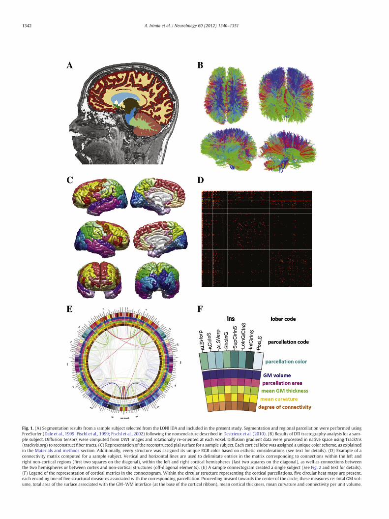
Fig. 1. (A) Segmentation results from a sample subject selected from the LONI IDA and included in the present study. Segmentation and regional parcellation were performed usingFreeSurfer (Dale et al., 1999; Fischl et al., 1999; Fischl et al., 2002) following the nomenclature described in Destrieux et al. (2010). (B) Results of DTI tractography analysis for a sam-ple subject. Diffusion tensors were computed from DWI images and rotationally re-oriented at each voxel. Diffusion gradient data were processed in native space using TrackVis(trackvis.org) to reconstruct fiber tracts. (C) Representation of the reconstructed pial surface for a sample subject. Each cortical lobe was assigned a unique color scheme, as explainedin the Materials and methods section. Additionally, every structure was assigned its unique RGB color based on esthetic considerations (see text for details). (D) Example of aconnectivity matrix computed for a sample subject. Vertical and horizontal lines are used to delimitate entries in the matrix corresponding to connections within the left andright non-cortical regions (first two squares on the diagonal), within the left and right cortical hemispheres (last two squares on the diagonal), as well as connections betweenthe two hemispheres or between cortex and non-cortical structures (off-diagonal elements). (E) A sample connectogram created a single subject (see Fig. 2 and text for details).(F) Legend of the representation of cortical metrics in the connectogram. Within the circular structure representing the cortical parcellations, five circular heat maps are present,each encoding one of five structural measures associated with the corresponding parcellation. Proceeding inward towards the center of the circle, these measures re: total GM vol-ume, total area of the surface associated with the GM–WM interface (at the base of the cortical ribbon), mean cortical thickness, mean curvature and connectivity per unit volume.

1342 A. Irimia et al. / NeuroImage 60 (2012) 1340–1351

Table 1Summary of each parcellation's abbreviation, full description and FreeSurfer code as defined in the original parcellation scheme (Destrieux et al., 2010), as well as the associatedRGB code in the connectogram.

Abbreviation Description FreeSurfer code RGB code

Neocortical structuresACgG/S Anterior part of the cingulate gyrus and sulcus G_and_S_cingul-Ant 255 255 180

ACirInS Anterior segment of the circular sulcus of the insula S_circular_insula_ant 102 255 255

ALSHorp Horizontal ramus of the anterior segment of the lateral sulcus (or fissure) Lat_Fis-ant-Horizont 0 255 204

ALSVerp Vertical ramus of the anterior segment of the lateral sulcus (or fissure) Lat_Fis-ant-Vertical 0 255 255

AngG Angular gyrus G_pariet_inf-Angular 0 255 0

AOcS Anterior occipital sulcus and preoccipital notch (temporo-occipital incisure) S_occipital_ant 51 51 255

ATrCoS Anterior transverse collateral sulcus S_collat_transv_ant 153 0 204

CcS Calcarine sulcus S_calcarine 102 153 255

CgSMarp Marginal branch (or part) of the cingulate sulcus S_cingul-Marginalis 255 192 201

CoS/LinS Medial occipito-temporal sulcus (collateral sulcus) and lingual sulcus S_oc-temp_med_and_Lingual 153 204 255

CS Central sulcus (Rolando's fissure) S_central 255 51 0

Cun Cuneus (O6) G_cuneus 0 153 255

FMarG/S Fronto-marginal gyrus (of Wernicke) and sulcus G_and_S_frontomargin 204 0 51

FuG Lateral occipito-temporal gyrus (fusiform gyrus, O4–T4) G_oc-temp_lat-fusifor 102 102 255

HG Heschl's gyrus (anterior transverse temporal gyrus) G_temp_sup-G_T_transv 102 0 102

InfCirInS Inferior segment of the circular sulcus of the insula S_circular_insula_inf 0 102 102

InfFGOpp Opercular part of the inferior frontal gyrus G_front_inf-Opercular 255 204 0

InfFGOrp Orbital part of the inferior frontal gyrus G_front_inf-Orbital 153 051 0

InfFGTrip Triangular part of the inferior frontal gyrus G_front_inf-Triangul 255 0 0

InfFS Inferior frontal sulcus S_front_inf 153 102 0

InfOcG/S Inferior occipital gyrus (O3) and sulcus G_and_S_occipital_inf 51 153 255

InfPrCS Inferior part of the precentral sulcus S_precentral-inf-part 255 153 0

IntPS/TrPS Intraparietal sulcus (interparietal sulcus) and transverse parietal sulci S_intrapariet_and_P_trans 51 255 51

InfTG Inferior temporal gyrus (T3) G_temporal_inf 255 0 255

InfTS Inferior temporal sulcus S_temporal_inf 204 0 153

JS Sulcus intermedius primus (of Jensen) S_interm_prim-Jensen 153 204 0

LinG Lingual gyrus, lingual part of the medial occipito-temporal gyrus (O5) G_oc-temp_med-Lingual 102 204 255

LOcTS Lateral occipito-temporal sulcus S_oc-temp_lat 153 153 255

LoInG/CInS Long insular gyrus and central insular sulcus G_Ins_lg_and_S_cent_ins 0 204 204

LOrS Lateral orbital sulcus S_orbital_lateral 102 0 0

MACgG/S Middle–anterior part of the cingulate gyrus and sulcus G_and_S_cingul-Mid-Ant 255 240 191

MedOrS Medial orbital sulcus (olfactory sulcus) S_orbital_med-olfact 255 102 0

MFG Middle frontal gyrus (F2) G_front_middle 255 255 051

MFS Middle frontal sulcus S_front_middle 255 153 51

MOcG Middle occipital gyrus (O2, lateral occipital gyrus) G_occipital_middle 0 204 244

MOcS/LuS Middle occipital sulcus and lunatus sulcus S_oc_middle_and_Lunatus 0 51 255

MPosCgG/S Middle–posterior part of the cingulate gyrus and sulcus G_and_S_cingul-Mid-Post 255 224 203

MTG Middle temporal gyrus (T2) G_temporal_middle 255 102 204

OcPo Occipital pole Pole_occipital 0 0 153

OrG Orbital gyri G_orbital 255 255 153

OrS Orbital sulci (H-shaped sulci) S_orbital-H_Shaped 255 204 204

PaCL/S Paracentral lobule and sulcus G_and_S_paracentral 204 255 153

PaHipG Parahippocampal gyrus, parahippocampal part of the medial occipito-temporalgyrus (T5)

G_oc-temp_med-Parahip 204 204 255

PerCaS Pericallosal sulcus (S of corpus callosum) S_pericallosal 255 164 200

POcS Parieto-occipital sulcus (or fissure) S_parieto_occipital 204 255 51

PoPl Polar plane of the superior temporal gyrus G_temp_sup-Plan_polar 204 153 255

PosCG Postcentral gyrus G_postcentral 204 255 204

PosCS Postcentral sulcus S_postcentral 153 255 0

PosDCgG Posterior–dorsal part of the cingulate gyrus G_cingul-Post-dorsal 255 175 201

PosLS Posterior ramus (or segment) of the lateral sulcus (or fissure) Lat_Fis-post 204 255 255

PosTrCoS Posterior transverse collateral sulcus S_collat_transv_post 51 102 255

PosVCgG Posterior–ventral part of the cingulate gyrus (isthmus of the cingulate gyrus) G_cingul-Post-ventral 255 208 202

PrCG Precentral gyrus G_precentral 204 102 0

PrCun Precuneus (medial part of P1) G_precuneus 204 255 0

RG Straight gyrus (gyrus rectus) G_rectus 255 204 153

SbCaG Subcallosal area, subcallosal gyrus G_subcallosal 255 153 200

SbCG/S Subcentral gyrus (central operculum) and sulci G_and_S_subcentral 255 102 153

SbOrS Suborbital sulcus (sulcus rostrales, supraorbital sulcus) S_suborbital 255 51 102

SbPS Subparietal sulcus S_subparietal 102 153 0

ShoInG Short insular gyri G_insular_short 51 255 204

SuMarG Supramarginal gyrus G_pariet_inf-Supramar 204 255 102

SupCirInS Superior segment of the circular sulcus of the insula S_circular_insula_sup 0 153 153

SupFG Superior frontal gyrus (F1) G_front_sup 255 102 102

SupFS Superior frontal sulcus S_front_sup 204 153 0

SupOcG Superior occipital gyrus (O1) G_occipital_sup 0 0 255

SupPrCS Superior part of the precentral sulcus S_precentral-sup-part 255 0 102

SupOcS/TrOcS Superior occipital sulcus and transverse occipital sulcus S_oc_sup_and_transversal 0 102 255

SupPL Superior parietal lobule (lateral part of P1) G_parietal_sup 153 255 153

SupTGLp Lateral aspect of the superior temporal gyrus G_temp_sup-Lateral 153 51 255

SupTS Superior temporal sulcus S_temporal_sup 204 51 255

TPl Temporal plane of the superior temporal gyrus G_temp_sup-Plan_tempo 153 0 153

TPo Temporal pole Pole_temporal 255 204 255

(continued on next page)

1343A. Irimia et al. / NeuroImage 60 (2012) 1340–1351

Table 1 (continued)

Abbreviation Description FreeSurfer code RGB code

Neocortical structuresTrFPoG/S Transverse frontopolar gyri and sulci G_and_S_transv_frontopol 255 153 153

TrTS Transverse temporal sulcus S_temporal_transverse 255 153 255

Subcortical structuresAmg Amygdala Amygdala 159 159 159

CaN Caudate nucleus Caudate 96 96 96

Hip Hippocampus Hippocampus 223 223 223

NAcc Nucleus accumbens Accumbens-area 128 128 128

Pal Pallidum Pallidum 64 64 64

Pu Putamen Putamen 32 32 32

Tha Thalamus Thalamus-proper 191 191 191

Cerebellar structureCeB Cerebellum Cerebellum–cortex 255 64 0

Midline structureBStem Brain stem Brain-stem 207 255 48

1344 A. Irimia et al. / NeuroImage 60 (2012) 1340–1351

elements representing the left (quadrants II–III) and right (quadrantsI, IV) cerebral hemispheres, each positioned symmetrically withrespect to the vertical axis. We name this representation a ‘connecto-gram’. The brain stem was positioned at the inferior extremity of theCircos ring because of it being the onlymidline structure. In this fashion,Circos' ability to display chromosomeswasmodified for lobar depiction,while its functionality for illustrating cytogenetic bands was usedinstead to represent cortical parcellations. As previously described,each parcellation was assigned a unique RGB color. A complete list ofparcellations, their abbreviations and associated RGB codes are provid-ed in Table 1. Parcellations were arrangedwithin each lobe in the orderof their location along the antero-posterior axis of the cortical surfaceassociated with the published FreeSurfer normal population atlas(Destrieux et al., 2010). To determine this ordering, the center of masswas computed for the GM surface portion associated with each parcel-lation, and the order of all parcellations was determined based on thelocations of these centers of mass as their distance from the frontalpole increased along the antero-posterior coordinate axis. Thus, parcel-lated regions are displayed on each of the left and right semicirclesof the connectogram in antero-posterior order, which makes thearrangement straightforward to interpret.

Connectivity representation

For subject-level connectograms, links were generated betweenany two parcellations whenever a WM tract existed between them.In population-level analyses, the former was done whenever therewas a non-vanishing probability for a WM tract to exist betweenthe two regions. Links were color-coded by the average fractionalanisotropy (FA) value associated with the fibers between the tworegions connected by the link, as follows. The lowest and highestFA values over all links (FAmin and FAmax, respectively) were first com-puted. For any given connection i where i=1, …, N (N being the totalnumber of connections), the FA value FAi associated with that connec-tion was normalized as FA′i=(FAi−FAmin) /(FAmax−FAmin), wherethe prime indicates the FAi value after normalization. After this nor-malization, FA′i values were distributed in the interval [0, 1], where0 corresponds to FAmin and 1 corresponds to FAmax. The interval[0, 1] was then divided into three subintervals (bins) of equal size,namely [0, 1/3], [1/3, 2/3], and [2/3, 1]. For every i=1, …, N, link iwas color-coded in either blue, green or red, depending on whetherits associated FA′i value belonged to the first, second, or third binabove, respectively. In addition to encoding FA in the link's color asdescribed, fiber count was also encoded as link transparency. Thus,within each of the three FA bins described, the link associated withthe highest fiber count within that bin was rendered as perfectly

opaque, whereas the link with the lowest fiber count was colored astransparent as possible without rendering it invisible. For example,the link with FA′i=1/3 was colored opaque blue, whereas the linkwith the lowest FA′i value was colored as faintest (most transparent)blue. Similarly, the link with FA′i=2/3 was colored opaque green, andthe link with the lowest value of FA′i greater than 1/3 was coloredfaintest green. The links associated with the lowest fiber countswere drawn first, and links with progressively larger fiber countswere drawn on top of the former. The process was successively repeat-ed by drawing links with higher fiber counts on top of links with lowerfiber counts. Thus, links associated with the largest fiber counts weredrawn on top of all other links. A sample connectogram created usingthe methods above is shown in Fig. 1(E). To represent directionalityinformation, links can be displayed such that they gradually changecolor from one extremity to the other in order to distinguish incomingfrom outgoing information. For example, a link transmitting informa-tion from region A to region B can be colored such that its extremityat A is red (outgoing information) and its extremity at B is blue (incom-ing information). The link would thus gradually change color along itslength from A to B, indicating directionality from the former to thelatter. In addition, the user can additionally select only one or severalparcellated regions for which links are displayed.

Representation of cortical metrics

Within the circular structure representing the cortical parcellations,five circular heatmapswere generated, each encoding one of five struc-tural measures associated with the corresponding parcellation. Pro-ceeding inward towards the center of the circle, these measures were:total GM volume, total area of the surface associated with the GM–

WM interface (at the base of the cortical ribbon), mean cortical thick-ness,mean curvature and connectivity per unit volume. For eachparcel-lation, the latter measure was computed as the number of fibers withendings within that parcellation divided by the total GM volume ofthe parcellation. For the subject-level analysis, these measures werecomputed over the entire volumetric (or areal, as appropriate) extentof each parcellation; for the population-level analysis, they were addi-tionally averaged over all subjects. Values for each structural measurewere encoded as colors, using a color scheme mapping that rangedfrom the minimum to the maximum of the data set. For example, thecortical thickness twith values ranging from tmin to tmaxwas normalizedas t1=(t−tmin)/(tmax− tmin). The latter value was mapped onto aunique color from the color map of choice. Thus, for example, hues atcolor map extremities correspond to tmin and tmax, as required. For sub-cortical structures, brain stem and cerebellum, three measures (area,thickness and curvature) were unavailable on a parcellation-by-

Table 2Abbreviations for cortical parcellations used in connectograms. Thisscheme unambiguously maps the correspondence between each word orprefix and the appropriate keyword (see Table 1 for a list of parcellations).

Abbreviation Keyword

A AnteriorAcc AccumbensAng AngularB BrainC CentralCa CallosalCau CaudateCc CalcarineCeB CerebellumCg CingulateCir CircularCla ClaustrumCo CollateralCun CuneusD DorsalF Frontal/fronto-Fu FusiformG Gyrus/gyriH HeschlHip Hippocampus/hippocampalHor HorizontalIn Insula/insularInf InferiorInt Intra-J JensenL Lateral/lobuleLin LingualLu Lunate/lunatusLo LongM MiddleMed MedialMar MarginalN NucleusOc Occipital/occipito-Op OpercularOr OrbitalP ParietalPa Para-Pal PallidumPer Peri-Pl PlanePo Pole/polarPos Posterior/post-Pr Pre-Pu Putamenp Partpl PlaneR RectusS Sulcus/sulciSb Sub-Sho ShortSu Supra-Sup SuperiorT TemporalTha ThalamusTr TransverseTri TriangularV Ventralver Vertical

1345A. Irimia et al. / NeuroImage 60 (2012) 1340–1351

parcellation basis; their corresponding heat map entries were conse-quently left blank. A detailed legend that outlines the representationof cortical metrics, as outlined above, is shown in Fig. 1(F).

Network analysis

Because network theory can provide essential insight into thestructural properties of cortical connectivity networks in both healthand disease (Sporns, 2011), several network metrics of particular sig-nificance were computed for each subject, starting with the degree of

each node. In our case, nodes were denoted by parcellated regionsand edges were represented by fiber tracts. The node degree is thenumber of edges connected to a node and its calculation has funda-mental impact uponmany networkmeasures; moreover, node degreedistributions are highly informative of network architecture. Theentry indexed by i and j in the distance matrix of the graph containsthe minimum length of the path connecting vertices i and j and wascomputed using the algebraic shortest paths algorithm (Rubinov andSporns, 2010). The node assortativity (Newman, 2002), i.e. the correla-tion coefficient for the degrees of neighboring nodes, was also com-puted in addition to the graph diameter, which is the largest entry inthe distance matrix. The eccentricity of a node is the greatest geodesicdistance between it and any other vertex, and can be thought of ashow far a node is from the node most distant from it in the network.A measure related to eccentricity is the graph radius, which is theminimum eccentricity of any vertex. To investigate local network seg-regation, the clustering coefficient (Fagiolo, 2007), transitivity, thecommunity structure and the modularity (Newman and Leicht, 2007)of the network were computed. Investigating network segregation isimportant because it can reveal how much information brain regionsexchange as well as the extent to which such regions remain structur-ally segregated from each other. The clustering coefficient is an ele-mentary measure of local segregation and measures the density ofconnections between a node's neighbors. The transitivity is a collec-tively normalized variant of the clustering coefficient which circum-vents the problem of disproportionate influence by low-degreenodes upon the clustering coefficient value. The community structure(Blondel et al., 2008) yields a subdivision of the network into non-overlapping groups of nodes in a manner that maximizes the numberof within-group edges, and minimizes the number of between-groupedges. Finally, modularity conveys the balance of density of within-and between-module connections, and represents another usefulmeasure of network segregation. To study network integration, thecharacteristic path length of the network was computed, which is theaverage of the entries in the distance matrix. A related and allegedlymore robust measure of integration is the global efficiency of the net-work (Latora andMarchiori, 2001), which is the average of the inverseof the distance matrix. The local efficiency is the global efficiency com-puted on the neighborhood of the node, and is related to the clusteringcoefficient. The network density is another useful measure which isequal to the fraction of present connections to possible connections.Finally, to grasp the effects of network influence and centrality, thenetwork participation coefficient (Guimera and Nunes Amaral, 2005)was calculated, which assesses the diversity of between-module con-nections. In addition, betweenness centrality (Brandes, 2001)was com-puted, which is the fraction of all shortest paths in the network thatcontains a given node. Nodeswith high values of betweenness central-ity participate in a large number of shortest paths. For each of themea-sures listed above, the mean and standard deviation were computedfor each subject. To compare the connectivity profile of a sample sub-ject against that of his/her population, themean value of eachmeasureover all vertices was standardized using the corresponding mean andstandard deviation of the means of that measure of the population,and Z scores were then computed for the sample subject.

Availability

The connectogram generation workflow is being made freelyavailable via the LONI Pipeline environment (pipeline.loni.ucla.edu).Details and a sample pipeline file are provided in the Supplementarymaterial.

Results

Fig. 2 illustrates the connectivity profile of a sample subjectdrawn from our normal population. To illustrate the capabilities of

Fig. 2. Connectogram for a sample subject. The outermost ring shows the various brain regions arranged by lobe (fr — frontal; ins — insula; lim — limbic; tem — temporal; par —parietal; occ— occipital; nc— non-cortical; bs— brain stem; CeB— cerebellum) and further ordered anterior-to-posterior. The color map of each region is lobe-specific and maps tothe color of each regional parcellation as shown in Fig. 1(C). The set of five rings (from the outside inward) reflect the measures listed in Fig. 1(F). For non-cortical regions, onlyaverage regional volume is shown. The links represent the computed degrees of connectivity between segmented brain regions. Links shaded in blue represent DTI tractographypathways in the lower third of the distribution of FA, green lines the middle third, and red lines the top third (see text for details). Circular color maps detail the scale for eachmetric. (For interpretation of the references to color in this figure legend, the reader is referred to the web version of this article.)

1346 A. Irimia et al. / NeuroImage 60 (2012) 1340–1351

our methodology, it is useful to discuss specific features of this con-nectivity profile as obviated by the connectogram. One such featureis the thick red link that connects the left and right superior frontalgyri (SupFG) in the connectogram. The fact that this link is coloredin red indicates, as explained in the previous section, that the fibertracts between these regions have mean FA values that are greaterthan 67% of all FA values in the entire brain. The complete opacityof the link (i.e. its full red color, compared to other links that are col-ored using transparent, light hues of red) indicates that, among allregions in the brain that are connected to each other, the right andleft gyri are linked to each other by connections that have a veryhigh fiber count compared to counts between any two regions. Inother words, other regions are connected by fibers that have lowercounts, with the exception of the connection between the brainstem and left and right cerebella, which also have particularly largefiber counts. All these results are to be expected given the largearea and spatial extent of the SupFG, which is colored in Fig. 1(C)using the same color as that of the outermost connectogram

segment associated with this structure in Fig. 2 (light pink, seeFig. 1(F) for the connectogram legend).

Proceeding inward towards the center of the circle, the next ringencodes the GM volume of each parcellation. In the case of theSupFG, the bright green displayed for both left and right gyri indi-cates that the GM volumes of these structures are (among) the larg-est among those of all parcellations, which is again expectable giventhe spatial extent of these anatomical structures. The next concentriccircle is encoding the total area of the parcellation, and in the case ofthe superior frontal gyri the associated color is bright yellow whichindicates, as expected, that these structures have some of the largestareas among all parcellations. The GM thickness (next concentric cir-cle) of the gyri is encoded by light green, which indicates that theirthickness is close to the average parcellation thickness. The meancurvature of the SupFG is revealed to be somewhat larger than aver-age, given that the encoded colors for both left and right gyri arelight orange hues. Finally, the degree of connectivity (depicted onthe innermost circle of the connectogram) is relatively low. This

1347A. Irimia et al. / NeuroImage 60 (2012) 1340–1351

measure, which represents the total count of fibers with endings inthe structure under consideration divided by the total surface areaof that structure, indicates that the SupFG has relatively low surfacedensity of fibers for the sample patient considered. Informationregarding the GM volume, parcellation area, mean GM thickness,mean curvature and degree of connectivity can be decoded forother regions from the connectogram using the color scaling dis-played in Fig. 2, in a manner analogous to that exemplified abovefor the SupFG. In conclusion, the discussion above highlights therichness of information that can be gathered visually from the con-nectogram about any cortical regions based on the color codingused.

Fig. 3. Connectograms of four subjects selected from the healthy population. Illustrated ardifferent subjects, which can be easily explored using our connectogram methodology.

An interesting feature of the connectogram in Fig. 2 is the asym-metry in the connectivity profile of the left SupFG compared to thatof the right SupFG. Specifically, the connections of the left SupFG tothe right subcallosal gyrus (SbCaG) and to the right middle posteriorcingulated gyrus and sulcus (MPosCgG/S) have higher fiber countsand larger FAs than the connections between the correspondingcontralateral structures (i.e. right SupFG to left SbCaG and to leftMPosCgG/S). This interesting characteristic associated with the con-nectivity profile of this subject is very easy to note from the connecto-gram, and highlights its usefulness in identifying patterns of eithersymmetry or asymmetry in the brain. Although it is not our purposehere to provide an exhaustive description of all connectivity patterns

e both the degrees of similarity and of variability between the connectivity profiles of

1348 A. Irimia et al. / NeuroImage 60 (2012) 1340–1351

in the selected subject in Fig. 2, suffice it to note that the connecto-gram approach is very useful for such type of undertaking, as wellas for exploring the connectivity profile of specific regions.

Whereas Fig. 2 displayed the connectivity profile of one samplesubject, Fig. 3 illustrates the connectivity profiles of four other sub-jects selected from our population. The purpose of this figure is tographically illustrate the degree of similarity as well as the variabilitybetween the connectivity profiles of different subjects, which can beeasily explored using our connectogram methodology. For all foursubjects presented, the left and right cerebella are linked by connec-tions that have large fiber counts and relatively low FA, whereasstructures that are part of the dorsolateral prefrontal cortex (e.g. pre-central and central gyri or sulci) are consistently linked to subcorticalstructures, creating a characteristic ‘V-shaped’ pattern in the connec-tograms. Careful visual investigations of these four connectogramsreveal other common patterns as well, but also a great degree ofvariability between subjects, not only in the fiber counts of variousconnections between regions but also in the FA values associatedwith them.

Fig. 4 displays the population-level connectogram pooled over all50 subjects included in our analysis using the methods already de-scribed. As expected given the process of averaging across subjects,

Fig. 4. As in Fig. 2, for the entire

this connectogram exhibits a greater degree of bilateral symmetrythan all other subject-specific connectograms already examined.Although some left–right asymmetry persists even here, it is reason-able to expect that either (A) some patterns of this type may disap-pear with the inclusion of additional subjects in the analysis, or(B) some asymmetry patterns may in fact be enhanced with increas-ing sample size. The latter would then suggest structural lateralitydifferences that are highly consistent over a very large population,and the methods of statistical analysis could then be employed toquantify the significance of such differences. Whereas it is not ourpurpose here to investigate how our population connectogrammight change upon inclusion of additional subjects, it is worthwhileto point out that our methodology is highly amenable to this type ofinvestigation. This is the case not only for healthy populations, butalso for clinical populations where connectomic analysis using ourapproach might allow one to obtain significant insights regardingthe structural connectivity profile in disease.

Although differences between control and target populations arenot explored in this study via connectogram design, it is useful todemonstrate our ability to perform statistical analyses using our par-adigm by comparing the cortical network properties of the subjectin Fig. 2 against the mean connectivity profile of his/her population,

population of 50 subjects.

Table 3Statistical comparison of the sample subject in Fig. 1 to the healthy population of adultsfrom which he/she was drawn. Listed are (1) the network measures computed, (2) themean of each network measure over all network nodes for the sample subject and forthe population, as well as (3) the Z score for the sample subject. Where measures aredesignated as binary in parentheses, the cortical network was assumed to be binary(i.e. with an edge weight of 1 if a connection existed between the nodes involved).Where measures are designated as weighted, the weight of each edge in the corticalnetwork was assumed to be equal to the fiber count associated with the connectionbetween nodes.

Network measure Mean Z score

Sample subject Population

Assortativity 0.004 0.027 0.694Betweenness (binary) 367.673 336.961 0.693Betweenness (weighted) 645.600 620.600 0.326Clustering coefficient (binary) 0.458 0.459 −0.051Clustering coefficient (weighted) 3.371 6.284 −0.861Community structure 4.630 4.977 −0.523Degree 8.315 10.477 −1.001Density 0.051 0.064 −1.001Diameter 7.000 6.392 0.783Distance (binary) 3.242 3.056 0.694Distance (weighted) 7.806 7.473 0.224Eccentricity 5.673 5.054 1.228Efficiency (global) 0.360 0.384 −0.794Efficiency (local) 0.656 0.682 −0.620Lambda 3.222 3.037 0.694Modularity 0.692 0.662 1.124Participation coefficient 0.288 0.303 −0.598Radius 4.000 3.451 0.642Transitivity (binary) 0.340 0.360 −0.614Transitivity (weighted) 2.495 5.001 −0.886

1349A. Irimia et al. / NeuroImage 60 (2012) 1340–1351

which is displayed in Fig. 4. To this end, Table 3 displays, for the sam-ple patient in Fig. 2, the mean values of the networkmetrics describedin the previous section, in addition to the values of the Z score associ-ated with each of these metrics for the sample subject, computed aspreviously described. Inspection of the Z scores in Table 3 indicatesthat, for all computed network metrics, the sample subject that wasselected for illustration was never farther away than 1.228 standarddeviations from the mean of the healthy population from which he/she was selected, indicating that this subject was quite typical of thepopulation from the standpoint of the cortical network measuresthat were calculated. This simple analysis of cortical measures inwhich a single subject was compared to an entire population usingthe standard measures of network theory can be used in conjunctionwith the analysis of the connectogram of the subject to gain insightinto his/her connectivity profile. It is quite possible that this type ofinvestigation can be useful especially when comparing a patient withany of the many clinical conditions that affect structural connectivity(e.g. traumatic brain injury (TBI), parkinsonism, dementia, etc.) to apopulation of matched healthy subjects or to other diseased subjects.Thus, the methodology outlined in this paper can be applied to a widevariety of case studies and even to the comparison of two differentpopulations, with potential relevance to many areas of neuroscience.

Discussion

Significance and innovation

With the intense interest in the in vivo mapping of human con-nectomics, as evident in the launching of the Human ConnectomeProject (HCP, www.humanconnectomeproject.org) by the NationalInstitutes of Mental Health and Aging, considerable effort has ariseninto techniques that graphically represent the interconnectednessof neural structures. Along with ongoing efforts to map populationlevel connectomics is an interest for clinical application to the indi-vidual subject or patient. Being able to graphically depict and assessdeviation from population-level averages is illustrative of damaged

or altered connectivity, as in the case of TBI. Such illustration can beessential for localizing compromised regional connectivity and forcharacterizing network-level changes in network efficiency resultingfrom cortical insult.

The use of summary graphical depictions has been strongly advo-cated as a means for clinicians to rapidly and succinctly examine pa-tient case, medication, and treatment histories at a glance (Powsnerand Tufte, 1994, 1997). Computations of network-level propertiesare a valuable means to assess efficiency and the ‘wiring costs’ neededto link spatially disparate brain regions (Bullmore et al., 2009). Inaddition, calculation of population average network metrics and oftheir degree of variation permits individualized connectomics com-parison. As noted above, this is of potentially great importancein the context of patients having degenerative disease (e.g. dementia,TBI, mental illness, etc.).

In this article, we have introduced a novel technique for the map-ping and visualization of population-level and individual human con-nectomics via an intuitive two-dimensional circular representation.We illustrate, in a population of subjects as well as in an instancedrawn from it, how this simple and elegant conceptual frameworkis well suited toward the organization, representation, and inspectionof brain connectivity in a visually-insightful and content-rich manner.Using combined MRI/DTI data acquisition and automatic imagesegmentation, we have described our approach for the extraction of148 cortical and 17 non-cortical anatomical parcellations using stan-dardized nomenclature, followed by the calculation of structuralanatomy metrics (volume, area, cortical thickness, curvature) for cor-tical regions. By combining these structural data with the connectivi-ty profile extracted from high-angular resolution DTI, we have beenable to generate detailed representations of regional geometry andconnectivity for each individual to assess and examine their statisticalproperties.

The graphical representation presented here differs from three-dimensional approaches which provide excellent renderings of nodesand their linkages in anatomical space (Bullmore and Sporns, 2009),and that when examined along with force-directed graphs illustrateclustering and relatedness (Hagmann et al., 2008). For example, theConnectome Viewer Toolkit (http://www.connectomeviewer.org) isan open source framework to analyze and interactively display connec-tomes in three dimensions using a variety of visualization options(Gerhard et al., 2011). The 3D nature of such graphs, while essentialfor the accurate illustration of relative anatomical proximity of networknodes, requires an interactive graphical user interface in which tomanipulate, orient, and examine degrees of connectivity within brainnetworks. These representations are sometimes difficult to include effi-ciently in journal articles or for examination in print due to their intrin-sic three-dimensional nature. Two-dimensional approaches have beenexplored (Bassett and Gazzaniga, 2011) in the form of wiring diagramsthat employ the classical representations of graph theory, and suchrepresentations are helpful for understanding network structure. How-ever, many of them do not provide additional insight into nodalneuroanatomy and can often be difficult to interpret or to exploredue to frequent, dense clustering of nodes throughout the two-dimensional spatial extent of the connectivity representation,as well as to the large number of graph edges, which can renderemerging properties of the system difficult to discern. As expandedin the following section, our representation overcomes many ofthese drawbacks and provides a useful method for connectomicvisualization.

To our knowledge, methods which are suitable for jointly repre-senting inter-regional connectivity in addition to regional anatomicalmetrics have not been widely examined. Moreover, the present meth-od is among the very few that allows one to explore cortical networkconnectivity in 2D format without the drawbacks of directly convert-ing 3D graphs into 2D images. Such drawbacks include, for example,the loss of significant information contained in the 3D structure of

1350 A. Irimia et al. / NeuroImage 60 (2012) 1340–1351

the representation, such as spatial positioning of nodes either closeror farther away from the user's viewpoint. By contrast, our presenttechnique makes use of its 2D, circular modality of display to elimi-nate the disadvantages that can be incurred as a 3D graph is con-verted to two dimensions for printing and inspection without therequirement of using a dedicated software package. In addition, theinclusion of edge transparency and the freedom of its manipulationby the user can be employed to highlight significant connectionsin their decreasing order of importance without compromising theoverall complexity of the graph structure.

Another important advantage of the present approach includessignificant potential for connectographic mapping and analysis acrosshuman samples, as well as an essentially unbounded capacity forextending this powerful analysis method to the study and compari-son of diseased populations and/or animal models, as described forexample in (Irimia et al., in press) Our methodology provides an ana-tomically informed arrangement of (1) nodal cortical and sub-corticalarchitecture, (2) their geometric properties, and (3) the degree andproperties of regional connectivity. Representing such informationhas not previously been performed within a single summary graphic.However, the information needed to create them is readily availablefrom workflow tools such as LONI Pipeline utilizing FreeSurfer, Track-Vis, etc. Thus, the representation presented here has similar qualitiesfor the ease for depicting and representing a complete set of connec-tomics information. The color-driven representation of neuroanatom-ical geometry as well as degree of inter-regional connectednessalso have a number of esthetic qualities — not the least of which is ahigh data-to-ink ratio (Tufte, 2001), e.g. maximizing scientific infor-mation content while minimizing superfluous graphical elements.In the following section, the innovative aspects of our circular repre-sentation framework are compared in more detail with the featuresof other methods employing either 2D or 3D representations. Theconnectogram software presented in this paper is freely availablefor download as an integrated module within the LONI Pipeline(pipeline.loni.ucla.edu, see also Dinov et al., 2010).

Comparison with other methods

Awide array of methodologies for the visualization of connectivityhas been proposed. Most of these representations rely on variationsof classical graph theory to (1) create and position network nodesat 3D locations associated with various anatomical landmarks,(2) represent nodes using shapes of various sizes and colors inorder to encode properties of interest, and to (3) modulate edgeproperties (weight, color, thickness, etc.) according to the degree ofconnectivity between nodes as expressed using some metricof choice. In the remainder of this subsection, these three modalitiesof visualization are discussed and analyzed from the perspectiveof existing methodologies and then compared to our own approachto emphasize the advantages and disadvantages of each framework.

The first task involved in connectomics visualization is that ofnode creating and positioning. One method of representation whichis very popular in this respect is illustrated in numerous publications(Bassett et al., 2011; Gerhard et al., 2011; Yan et al., 2011), wherenodes are positioned at the 3D anatomical coordinates of anatomicalbrain regions, and connection strengths are represented by edgethickness. This modality of representing brain connectivity has theadvantage that, when viewed in three dimensions, it allows one to as-sociate underlying neuroanatomy with precisely the locations of theregions of interest involved in the connectivity representation. An im-portant disadvantage of this method is that it can sometimes makeemergent network structure very difficult to grasp (Sanz-Arigitaet al., 2010). By comparison, our proposed visualization paradigmarranges nodes in their order along the antero-posterior axis (whichpreserves the logical spatial ordering of the parcellated regions),although it omits their precise 3D coordinates. However, even in

doing so, our method provides the capability of making all nodesequally visible to the viewer when the connectogram is inspectedon the printed page or outside any software environment that in-volves the manipulation of perspective in three dimensions for thepurpose of detailed inspection. In fairness, it should be noted that2D visualization of brain networks where node positioning followsexact anatomical positioning is in fact possible if the cortical surfaceis spread out as a 2D sheet, as for example in (Palva et al., 2010) orusing certain parameter options of the Connectome Viewer software(Gerhard et al., 2011). However, such representations remain atleast partially problematic because of the difficulty to associate arbi-trary locations on 2D flattened maps of the cortex to the familiar 3Dtopology of the brain. By contrast, our circular scheme follows theconventional antero-posterior positioning of nodes, thus creating amore intuitive 2D visualization of network structure.

The second challenge which must be addressed to visualize a con-nectome diagrammatically is that of depicting nodes using visualsymbols that are representative of their properties. For example, in(Chen et al., 2011; Dosenbach et al., 2007; Ginestet and Simmons,2011; Spoormaker et al., 2010) and many other publications, nodesare depicted as circles or spheres that are colored differently toencode various properties. One advantage of this modality of visuali-zation is that it allows one to easily grasp common edge properties, aswell as to visually classify nodes into classes according to their color-ing. Disadvantages of this method include the fact that nodes that arevery close to each other may visually overlap edges or each other,thus making graph structure more difficult to decipher and interpret.This problemmay be partially addressed by modifying node transpar-ency (Ginestet and Simmons, 2011), although this does not entirelyremove the difficulty of depicting cortical networks with high densi-ties of nodes or edges. By contrast to these methods, ours ensuresthat all nodes are simultaneously visible. In addition, our connecto-gram approach allows one to display an arbitrary number of nodeproperties at a time through the use of color-coded rings that are con-centric to the outermost circle.

The third difficulty involved in depicting connectomics relation-ships schematically involves the modulation of edge properties(weight, color, thickness, etc.) according to the degree of connectivitybetween nodes as expressed using somemetric of choice. In many ap-plications, edges are modulated by color (Cao and Slobounov, 2010;van den Heuvel and Pol, 2010) or by thickness (He and Evans, 2010;He et al., 2010). In one widely-disseminated approach similar toours in its use of a circular diagram (Holten, 2006; Modha andSingh, 2010), concentric circles are used to represent the hierarchicalsubdivision of the central nervous system in a top–down approach(e.g. brain to cortex to lobes to gyral/sulcal structures, etc.). In suchrepresentations, edges radiate from the center of a circle (the topstructure) to the circumference (the lowest-level structures) andedge position in the hierarchy is consequently important. In this lastapproach as well as in ours, the circular shape of the connectivitygraph is appealing and useful for the 2D representation of relation-ships between different areas of the brain. One challenge that thecircular approach to connectome viewing addresses is that of com-plexity and dimensionality reduction. In the hierarchical approach(Holten, 2006; Modha and Singh, 2010), this is addressed via thetop–down organization of connections; in ours, it can be controlledby displaying connections emanating only from one hemisphere,one lobe, or from a single brain structure, thus allowing the usergreat leeway in the ability to modify the level of complexity beingdisplayed in the connectogram.

Conclusion

Circle-based arrangements for connectome visualization are in-creasingly gaining acceptance in neuroimaging and computationalneuroscience circles (Modha and Singh, 2010). While many examples

1351A. Irimia et al. / NeuroImage 60 (2012) 1340–1351

of connectomic and network-level layouts have been proposed, theapproach described here for the joint 2D graphical representation ofregional geometric attributes and inter-regional connectivity is anovel, informative, and attractive means for depicting whole brainconnectivity from neuroimaging data. It allows for single subject aswell as population-level rendering and is complimentary to computa-tions of network architecture. The manner in which we envision thepotential contribution of our proposed method to existing visualiza-tion tools for connectomics is by complementing existing softwaremethodologies for mapping the highly complex networks of the cor-tex, such as the Connectome Viewer. In introducing the present visu-alization method, our purpose is to acknowledge the strengths andweaknesses of various other methods for depicting connectomics,and consequently to complement them in a constructive mannerthat is beneficial to members of the community who use such tools.In conclusion, our depiction of structural and connectivity data high-lights the detailed richness of connectome-related information,which is often challenging to visualize and interpret. Consequently,we expect our representation to have appreciable applicability tothe study of both population- and patient-level connectivity.

Supplementary materials related to this article can be foundonline at doi:10.1016/j.neuroimage.2012.01.107.

Disclosure statement

None of the authors has a conflict of interest to disclose.

Acknowledgments

We acknowledge the assistance of the staff of the Laboratory ofNeuro Imaging at the University of California, Los Angeles. Thiswork was supported by the National Alliance for Medical Image Com-puting (NA-MIC; www.na-mic.org), under NIH Roadmap Initiativegrant 2U54EB005149, sub-award to J. D. V. H.

References

Bassett, D.S., Gazzaniga, M.S., 2011. Understanding complexity in the human brain.Trends Cogn. Sci. 15, 200–209.

Bassett, D.S., Brown, J.A., Deshpande, V., Carlson, J.M., Grafton, S.T., 2011. Conservedand variable architecture of human white matter connectivity. Neuroimage 54,1262–1279.

Blondel, V.D., Guillaume, J.-L., Lambiotte, R., Lefebvre, E., 2008. Fast unfolding of com-munities in large networks. J. Stat. Mech.: Theory Exp. P10008.

Brandes, U., 2001. A faster algorithm for betweenness centrality. Journal of Mathemat-ical Sociology 25, 163–177.

Bullmore, E., Sporns, O., 2009. Complex brain networks: graph theoretical analysis ofstructural and functional systems. Nat. Rev. Neurosci. 10, 186–198.

Bullmore, E., Barnes, A., Bassett, D.S., Fornito, A., Kitzbichler, M., Meunier, D., Suckling,J., 2009. Generic aspects of complexity in brain imaging data and other biologicalsystems. Neuroimage 47 (3), 1125–1134.

Cao, C., Slobounov, S., 2010. Alteration of cortical functional connectivity as a result oftraumatic brain injury revealed by graph theory, ICA, and sLORETA analyses of EEGsignals. IEEE Trans. Neural Syst. Rehabil. Eng. 18, 11–19.

Chen, H.F., Liao, W., Ding, J.R., Marinazzo, D., Xu, Q.A., Wang, Z.G., Yuan, C.P., Zhang, Z.G.,Lu, G.M., 2011. Small-world directed networks in the human brain: multivariateGranger causality analysis of resting-state fMRI. Neuroimage 54, 2683–2694.

Chiang, M.C., Barysheva, M., Toga, A.W., Medland, S.E., Hansel, N.K., James, M.R.,McMahon, K.L., de Zubicaray, G.I., Martin, N.G., Wright, M.J., Thompson, P.M.,2011. BDNF gene effects on brain circuitry replicated in 455 twins. Neuroimage55, 448–454.

Dale, A.M., Fischl, B., Sereno, M.I., 1999. Cortical surface-based analysis — I. Segmenta-tion and surface reconstruction. NeuroImage 9, 179–194.

Darwin, C., 1859. On the Origin of Species by Means of Natural Selection. John Murray,London, UK.

Destrieux, C., Fischl, B., Dale, A., Halgren, E., 2010. Automatic parcellation of human cor-tical gyri and sulci using standard anatomical nomenclature. Neuroimage 53, 1–15.

Dinov, I., Lozev, K., Petrosyan, P., Liu, Z., Eggert, P., Pierce, J., Zamanyan, A., Chakrapani,S., Van Horn, J., Parker, D.S., Magsipoc, R., Leung, K., Gutman, B., Woods, R., Toga, A.,2010. Neuroimaging study designs, computational analyses and data provenanceusing the LONI pipeline. PLoS One 5.

Dosenbach, N.U.F., Fair, D.A., Miezin, F.M., Cohen, A.L., Wenger, K.K., Dosenbach, R.A.T.,Fox, M.D., Snyder, A.Z., Vincent, J.L., Raichle, M.E., Schlaggar, B.L., Petersen, S.E.,2007. Distinct brain networks for adaptive and stable task control in humans.Proc. Natl. Acad. Sci. U. S. A. 104, 11073–11078.

Fagiolo, G., 2007. Clustering in complex directed networks. Phys. Rev. E Stat. Nonlin.Soft Matter Phys. 76, 026107.

Fischl, B., Sereno, M.I., Dale, A.M., 1999. Cortical surface-based analysis — II: Inflation,flattening, and a surface-based coordinate system. Neuroimage 9, 195–207.

Fischl, B., Salat, D.H., Busa, E., Albert, M., Dieterich, M., Haselgrove, C., van der Kouwe,A., Killiany, R., Kennedy, D., Klaveness, S., Montillo, A., Makris, N., Rosen, B., Dale,A.M., 2002. Whole brain segmentation: automated labeling of neuroanatomicalstructures in the human brain. Neuron 33, 341–355.

Gerhard, S., Daducci, A., Lemkaddem, A., Meuli, R., Thiran, J., Hagmann, P., 2011. TheConnectome Viewer Toolkit: an open source framework to manage, analyze, andvisualize connectomes. Front. Neuroinformatics 5, 1–15.

Ginestet, C.E., Simmons, A., 2011. Statistical parametric network analysis of functionalconnectivity dynamics during a working memory task. Neuroimage 55, 688–704.

Guimera, R., Nunes Amaral, L.A., 2005. Functional cartography of complex metabolicnetworks. Nature 433, 895–900.

Hagman, P., 2005. From Diffusion MR to Brain Connectomics. Informatics and Commu-nications. Federal Politechnical School of Lausanne, Lausanne, p. 141.

Hagmann, P., Cammoun, L., Gigandet, X., Meuli, R., Honey, C.J., Wedeen, V., Sporns, O.,2008. Mapping the structural core of human cerebral cortex. PLoS Biol. 6, 1479–1493.

Hagmann, P., Cammoun, L., Gigandet, X., Gerhard, S., Grant, P.E., Wedeen, V., Meuli, R.,Thiran, J.P., Honey, C.J., Sporns, O., 2010. MR connectomics: principles and chal-lenges. J. Neurosci. Methods 194, 34–45.

He, Y., Evans, A., 2010. Graph theoretical modeling of brain connectivity. Curr. Opin.Neurol. 23, 341–350.

He, Y., Lo, C.Y., Wang, P.N., Chou, K.H., Wang, J.H., Lin, C.P., 2010. Diffusion tensor trac-tography reveals abnormal topological organization in structural cortical networksin Alzheimer's disease. J. Neurosci. 30, 16876–16885.

Holten, D., 2006. Hierarchical edge bundles: visualization of adjacency relations inhierarchical data. IEEE Trans. Vis. Comput. Graph. 12, 741–748.

Irimia, A., Chambers, M.C., Torgerson, C.M., Filippou, M., Hovda, D.A., Alger, J.R., Gerig,G., Toga, A.W., Vespa, P.M., Kikinis, R., Van Horn, J.D., 2012. Patient-tailored connec-tomics visualization for the assessment of white matter atrophy in traumatic braininjury. Front. Neur. 3:10. doi:10.3389/fneur.2012.00010.

Krzywinski, M., Schein, J., Birol, I., Connors, J., Gascoyne, R., Horsman, D., Jones, S.J.,Marra, M.A., 2009. Circos: an information aesthetic for comparative genomics.Genome Res. 19, 1639–1645.

Latora, V., Marchiori, M., 2001. Efficient behavior of small-world networks. Phys. Rev.Lett. 87, 198701.

Modha, D.S., Singh, R., 2010. Network architecture of the long-distance pathways in themacaque brain. Proc. Natl. Acad. Sci. U. S. A. 107, 13485–13490.

Mori, S., Crain, B.J., Chacko, V.P., van Zijl, P.C.M., 1999. Three-dimensional tracking of axonalprojections in the brain by magnetic resonance imaging. Ann. Neurol. 45, 265–269.

Newman, M.E., 2002. Assortative mixing in networks. Phys. Rev. Lett. 89, 208701.Newman, M.E., Leicht, E.A., 2007. Mixture models and exploratory analysis in net-

works. Proc. Natl. Acad. Sci. U. S. A. 104, 9564–9569.Palva, J.M., Monto, S., Kulashekhar, S., Palva, S., 2010. Neuronal synchrony reveals

working memory networks and predicts individual memory capacity. Proc. Natl.Acad. Sci. U. S. A. 107, 7580–7585.

Powsner, S.M., Tufte, E.R., 1994. Graphical summary of patient status. Lancet 344, 386–389.Powsner, S.M., Tufte, E.R., 1997. Summarizing clinical psychiatric data. Psychiatr. Serv.

48, 1458–1461.Rubinov, M., Sporns, O., 2010. Complex network measures of brain connectivity: uses

and interpretations. Neuroimage 52, 1059–1069.Sanz-Arigita, E.J., Schoonheim, M.M., Damoiseaux, J.S., Rombouts, S.A.R.B., Maris, E.,

Barkhof, F., Scheltens, P., Stam, C.J., 2010. Loss of ‘small-world’networks inAlzheimer'sdisease: graph analysis of fMRI resting-state functional connectivity. PLoS One 5.

Sneath, P.H.A., 1957. The application of computers to taxonomy. J. Gen. Microbiol. 17,201–226.

Spoormaker, V.I., Schroter, M.S., Gleiser, P.M., Andrade, K.C., Dresler, M., Wehrle, R.,Samann, P.G., Czisch, M., 2010. Development of a large-scale functional brain net-work during human non-rapid eye movement sleep. J. Neurosci. 30, 11379–11387.

Sporns, O., 2011. Networks of the Brain. The MIT Press, Cambridge, MA.Sporns, O., Tononi, G., Kotter, R., 2005. The human connectome: a structural description

of the human brain. PLoS Comput. Biol. 1, 245–251.Tufte, E., 2001. The Visual Display of Quantitative Information, Second ed. Graphics

Press, Cheshire, CT.van den Heuvel, M.P., Pol, H.E.H., 2010. Exploring the brain network: a review on

resting-state fMRI functional connectivity. Eur. Neuropsychopharmacol. 20,519–534.

Yan, C., Gong, G., Wang, J., Wang, D., Liu, D., Zhu, C., Chen, Z.J., Evans, A., Zang, Y., He, Y.,2011. Sex- and brain size-related small-world structural cortical networks inyoung adults: a DTI tractography study. Cereb. Cortex 21, 449–458.