Connecting Algebra and Biology Using Graphing … Algebra and Biology Using Graphing Calculators...
132
Connecting Algebra and Biology Using Graphing Calculators Activities Using the TI-83 and Casio 9850 G Plus Office of Secondary Instructional Services Virginia Department of Education P.O. Box 2120 Richmond, Virginia 23218-2120 April 1999
Transcript of Connecting Algebra and Biology Using Graphing … Algebra and Biology Using Graphing Calculators...
Connecting Algebra and BiologyUsing Graphing Calculators
Activities Using theTI-83 and Casio 9850 G Plus
Office of Secondary Instructional ServicesVirginia Department of Education
P.O. Box 2120Richmond, Virginia 23218-2120
April 1999

Virginia Department of Education i Connecting Algebra and biology
COMMONWEALTH OF VIRGINIADEPARTMENT OF EDUCATION
Superintendent of Public InstructionPaul D. Stapleton
Deputy SuperintendentM. Kenneth Magill
Assistant Superintendent for InstructionJo Lynne DeMary
Office of Secondary Instructional Services
Patricia I. WrightDirector
Maureen B. HijarMathematics Specialist
Delores DaltonScience Specialist
Virginia Department of Education ii Connecting Algebra and biology
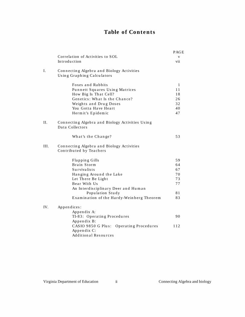
Table of Contents
PAGECorrelation of Activities to SOL vIntroduction vii
I. Connecting Algebra and Biology ActivitiesUsing Graphing Calculators
Foxes and Rabbits 1Punnett Squares Using Matrices 11How Big Is That Cell? 18Genetics: What Is the Chance? 26Weights and Drug Doses 32You Gotta Have Heart 40Hermit’s Epidemic 47
II. Connecting Algebra and Biology Activities UsingData Collectors
What’s the Change? 53
III. Connecting Algebra and Biology ActivitiesContributed by Teachers
Flapping Gills 59Brain Storm 64Survivalists 67Hanging Around the Lake 70Let There Be Light 73Bear With Us 77An Interdisciplinary Deer and Human
Population Study 81Examination of the Hardy-Weinberg Theorem 83
IV. Appendices:Appendix A:TI-83: Operating Procedures 90Appendix B:CASIO 9850 G Plus: Operating Procedures 112Appendix C:Additional Resources
Virginia Department of Education iii Connecting Algebra and biology
Correlation of Activities to SOL
Name of Activity Related SOL Page NumberFoxes and Rabbits BIO.1, BIO.5, BIO.8,
BIO.9; A.51
Punnett Squares UsingMatrices BIO.1, BIO.6; A.4
11
How Big Is That Cell? BIO.4, BIO.6; A.5 18Genetics: What is theChance?
BIO.1, BIO.6; A.18 26
Weights and Drug Doses BIO.1, BIO.2, BIO.4,BIO.5; A.17
32
You Gotta Have Heart BIO.1, BIO.5; A.18 40The Hermit’s EpidemicWhat's the Change?
BIO.1, BIO.5; A.18BIO.1, BIO.3, A.17
4753
Flapping Gills BIO.1, BIO.5; A.17 59Brain Storm BIO.1, BIO.2, BIO.8,
BIO.9; A.7, A.15, A.1764
Survivalist BIO.8; A.17 67Hanging Around theLake
BIO.1, BIO.2, BIO.3,BIO.4, BIO.5, BIO.7,BIO.9; A.7, A.17
70
Let There Be Light BIO.1, BIO.8, BIO.9; A.7 73Bear With Us BIO.1, BIO.8, BIO.9;
A.17, A.1877
Deer and HumanPopulation Study
BIO.1, BIO.8, BIO.9; A.5,A.18
81
Examination of Hardy-Weinberg Theorem
BIO.1, BIO.6, BIO.8; A.5 83

Virginia Department of Education iv Connecting Algebra and biology
Introduction
The Connecting Algebra and Biology Using Graphing Calculatorsresource document is intended to assist classroom teachers of algebraand biology in implementing the Virginia Standards of Learning formathematics and science. This resource document includes a samplingof activities that have been correlated to the Standards of Learning forAlgebra I, Algebra II, and Biology. Where appropriate, activities have alsobeen correlated to Standards of Learning for other grade levels orcourses.
The purpose of this resource document is to enhance theimplementation of the Mathematics and Science Standards of Learning,especially in algebra, biology, data analysis, applications, andtechnology. The content of the activities focuses on algebra, statistics,and data analysis with applications from biology. The activities requirestudents to use graphing calculators, data collecting devices, and/orscientific probes to investigate and solve problems. The scientificinvestigations require the use of algebra and data analysis. Thus,students will learn connections between algebra and biology contentwhile solving application problems and using the technology required inthe Standards of Learning.
The activities in this resource document were field tested andedited by classroom teachers. Each activity has been written for usewith both the Texas Instruments-(TI) 83 and the Casio 9850 G Plusgraphing calculators. The document also includes activities for use withthe following scientific probe kits that interface with the graphingcalculators: Texas Instruments Calculator-Based Laboratory (CBL) andthe Casio EA-100 Data Analyzer. A special section includes activitieswritten by classroom teachers of algebra and biology during a ConnectingAlgebra and Biology summer institute, which was sponsored by theVirginia Department of Education in 1997. Contributing teachers’names are listed on the activities.
To assist teachers who have had limited training or experience inusing graphing calculators, operating procedures for the TI-83 and Casio9850 G Plus graphing calculators are included in the appendix. Theseinstructions are not intended to be comprehensive. They are intended asa starting point for teachers who want to begin immediately using theactivities. The instructions focus on the data analysis procedures thatthe activities require.

Virginia Department of Education v Connecting Algebra and Biology
The materials in this document may be duplicated and distributed asdesired for use in Virginia. The Virginia Department of Education will provideschool divisions with additional information to be included in this document asother resources are identified. School divisions are also encouraged to addappropriate activities and resource materials to this document.
The Connecting Algebra and Biology Using Graphing Calculators resourcedocument is being provided to school divisions through an appropriation fromthe General Assembly and in accordance with the Virginia Department ofEducation’s responsibility to develop and pilot model teacher, principal, andsuperintendent training activities geared to the Standards of Learning contentand assessments, and to technology applications.
Acknowledgments
The Virginia Department of Education wishes to express sincereappreciation to the following individuals who contributed to the writing andediting of the activities in this document.
Maureen Hijar Virginia Department of
Education
Patti Kemp Prince William County
Anne Kapral Virginia Beach City
Jill Lossee-Hoehlin Chesapeake City Schools
Patricia Maturo Fairfax County
Kathleen Stoebe Prince William
Verle Walters Norfolk City

Virginia Department of Education 3 Connecting Algebra and Biology
Foxes and Rabbits
Related SOL: BIO.1, BIO.5, BIO.8, BIO.9, and A.5
Overview Predators are organisms that feed upon other living things called prey.
The effect of this interaction on the health and welfare of both the predator and prey populations can be seen in this representative simulation. The simulation will use a fox to represent the predator and rabbits to represent the prey.
Problem StatementHow does the predator /prey relationship affect the growth of eachpopulation?
Materialmasking tape fox (1 large weighted square)meter stick data chartrabbits (300 small squares) graphing calculator
Procedure and Data
What is your prediction (hypothesis) about the predator-prey relationship?
1. Construct a square that is 70 centimeters on each side on a tabletopusing masking tape to mark the boundaries. This is your woodland.
2. Use the chart provided to record your data. A suggestion to simplify recording procedures is to keep tally marks on a separate piece of paper until all foxes of a generation are tossed, and then enter the numbers on the data chart.
3. Generation 1 consists of three rabbits and one fox.
4. Toss three rabbits into the square (your woodland).

Virginia Department of Education 4 Connecting Algebra and Biology
5. Stand one meter from the table. Toss the fox into the large square. Eachtoss will represent one fox. Try to land on as many rabbits as possible.After the fox lands, any rabbit it touches will be considered captured.Count the captured rabbits and remove them.
6. Tally the following information based on the number of rabbitscaptured:
ü Tally the number of captured rabbits.
ü If the fox catches fewer than three rabbits, it starves to death. Placea tally mark in the fox starvation column.
ü If the fox catches three or more rabbits, place a tally mark in the foxsurvival column.
ü Determine the number of offspring produced by your fox by dividingthe number of rabbits captured by 3. Record only the whole numberof offspring with a tally mark in the fox birth column; DO NOTROUND. For example, six, seven, or eight rabbits captured by onefox will support fox offspring.
ü Determine the number of rabbits and foxes for the next generation.
ü To calculate the number of foxes that will make up your nextgeneration, add the fox survival and fox birth columns. Enter thisdata in the start column of the next generation.
ü If zero foxes are left to begin the next generation, a new fox moves infrom a new woodland, so enter “1” in the start column of the nextgeneration.
ü Calculate the number of rabbits remaining by subtracting the rabbitscaptured column from the rabbit start column. Enter this number inthe rabbits remaining column.
Virginia Department of Education 5 Connecting Algebra and Biology
ü Each rabbit remaining will produce an average of two offspring. Tocalculate the number of rabbits that will make up the nextgeneration, multiply the number of remaining rabbits by “3”. Thiswill account for the current generation’s rabbits that survive, as wellas their offspring. For example, if 4 rabbits remained after all of thefoxes were tossed, your next generation will begin with 12 rabbits,since 4 x 3 = 12. Enter your result in the start column of the nextgeneration.
ü The woodland vegetation can support no more that 300 rabbits. Ifyour rabbit population reaches or exceeds 300, enter “300” in therabbit start column of the next generation.
ü If zero rabbits are left to begin the next generation, a new rabbitfamily moves into the woodland, so enter “1” in the start column ofthe next generation.
7. Determine the start values for generations 1 through 7. Stop here fordata interpretation.
Refer to the CASIO or TI information now.
8. Now repeat the activity for generations 8 through 14.
Refer to the CASIO or TI information now.

Virginia Department of Education 6 Connecting Algebra and Biology
Analysis:
1. Compare the actual model to the predictions for generations 8, 11 and 14. How arethey similar or different?
Similarities Differences
________________________ ________________________
________________________ ________________________
2. What do you think would be the population of rabbits and foxes after 20 generations? _____________ 30 generations? _____________
3. Name two reasons for the differences.a. ______________________ b. __________________________
4. What do you think would happen to the rabbit population if all the foxes were trapped for their fur? Name at least two things. a. ___________________________________________________________
b. ___________________________________________________________
5. What do you think would happen to the fox population if the rabbits caught a lethal disease such as pneumonia? Name at least two things. a. ___________________________________________________________
b. ___________________________________________________________
6. Why do you think the population graph fluctuates?
7. What other factors may affect the balance of each population? Name at least three.a. __________________ b. __________________ c. ___________________
8. If you were a chicken and vegetable farmer, write a short essay to explain why you would or would not support a bounty on foxes in your area. Be sure to state both pros and cons to your argument.
Virginia Department of Education 7 Connecting Algebra and Biology
CASIO 9850 G+ Graphing Information
1. On your graphing calculator, plot the starting populations of rabbits and foxesusing one symbol for rabbits and another for foxes.
Go to STAT Mode (#2). Make sure to clear all previous lists.
Enter into List 1 the generation numbers, 1 through 14. Enter into List 2 thestarting number of rabbits for each of the 7 generations you have calculated thusfar. Enter into List 3 the starting number of foxes for each of the 7 generationsyou have calculated thus far.
Press F1 (GRPH). Press F6 (SET). Set StatGraph1 as a scatter plot for therabbits. Highlight Graph Type, and press F1 (Scat). Highlight XList, and press F1(List 1). Highlight YList, and press F2 (List 2). Highlight Frequency, and press F1(1). For the last two settings, make your own choices. Just remember what yourchoices were so that you make different choices when making a scatter plot forthe foxes. Press the EXE key.
Press F6 (SET). Press F2 (GPH2). Set StatGraph2 as a scatter plot for the foxes.Highlight Graph Type, and press F1 (Scat). Highlight XList, and press F1 (List 1).Highlight YList, and press F3 (List 3). Highlight Frequency, and press F1 (1). Forthe last two settings, make your own choices keeping in mind that you want adifferent mark type and graph color than what you chose for the rabbit scatterplot. Press the EXE key.
Press F4 (SEL). To compare the scatter plot for the rabbits and the scatter plot forthe foxes, StatGraph1 and StatGraph2 must both say, “DrawOn” and StatGraph3must say, “DrawOff”. Press F6 (DRAW). Utilize the Trace function to help youanalyze the data. To do this, press the yellow SHIFT key and then F1 (Trace).Use the up and down arrow keys to go back and forth between the data of thedifferent scatter plots. Use the left and right arrow keys to trace the data alongeach scatter plot.
2. From the graphs, make some predictions for the populations of generations 8, 11,and 14.
Go to STAT Mode (#2). Finish inputting your rabbit data into List 2 and your foxdata into List 3. Press F1 (GRPH). Press F4 (SEL). Make sure StatGraph1 andStatGraph2 are on, and StatGraph3 is off. Press F6 (DRAW).
Virginia Department of Education 8 Connecting Algebra and Biology
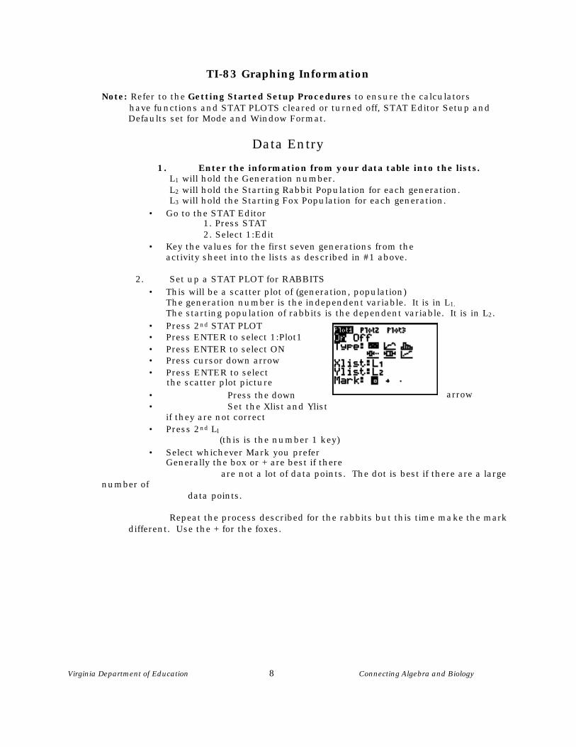
TI-83 Graphing Information
Note: Refer to the Getting Started Setup Procedures to ensure the calculators have functions and STAT PLOTS cleared or turned off, STAT Editor Setup and Defaults set for Mode and Window Format.
Data Entry
1. Enter the information from your data table into the lists. L1 will hold the Generation number.
L2 will hold the Starting Rabbit Population for each generation. L3 will hold the Starting Fox Population for each generation.
• Go to the STAT Editor 1. Press STAT
2. Select 1:Edit• Key the values for the first seven generations from the
activity sheet into the lists as described in #1 above.
2. Set up a STAT PLOT for RABBITS
• This will be a scatter plot of (generation, population)The generation number is the independent variable. It is in L1.
The starting population of rabbits is the dependent variable. It is in L2.
• Press 2nd STAT PLOT• Press ENTER to select 1:Plot1• Press ENTER to select ON• Press cursor down arrow• Press ENTER to select the scatter plot picture
• Press the down arrow• Set the Xlist and Ylist
if they are not correct• Press 2nd L1
(this is the number 1 key)
• Select whichever Mark you preferGenerally the box or + are best if there
are not a lot of data points. The dot is best if there are a largenumber of
data points.
Repeat the process described for the rabbits but this time make the mark different. Use the + for the foxes.
Virginia Department of Education 9 Connecting Algebra and Biology
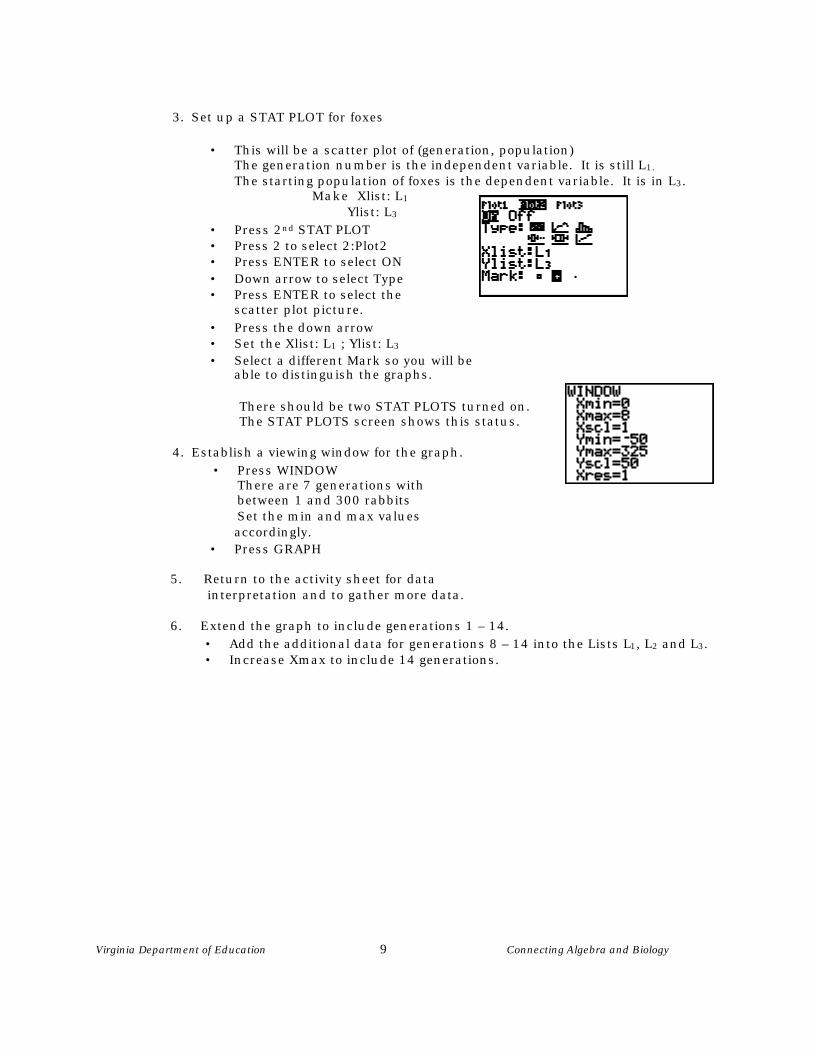
3. Set up a STAT PLOT for foxes
• This will be a scatter plot of (generation, population)The generation number is the independent variable. It is still L1.
The starting population of foxes is the dependent variable. It is in L3. Make Xlist: L1
Ylist: L3
• Press 2nd STAT PLOT• Press 2 to select 2:Plot2• Press ENTER to select ON• Down arrow to select Type• Press ENTER to select the
scatter plot picture.
• Press the down arrow• Set the Xlist: L1 ; Ylist: L3
• Select a different Mark so you will beable to distinguish the graphs.
There should be two STAT PLOTS turned on. The STAT PLOTS screen shows this status.
4. Establish a viewing window for the graph.
• Press WINDOWThere are 7 generations withbetween 1 and 300 rabbitsSet the min and max valuesaccordingly.
• Press GRAPH
5. Return to the activity sheet for data interpretation and to gather more data.
6. Extend the graph to include generations 1 – 14.
• Add the additional data for generations 8 – 14 into the Lists L1, L2 and L3.• Increase Xmax to include 14 generations.

Virginia Department of Education 10 Connecting Algebra and Biology
7. Activity Sheet Conclusion:In considering the predator-prey relationship it is interesting to view the graphof the rabbit population vs the fox population.
Turn off the previous Plots
• Press 2nd STAT PLOT • Press 4: PlotsOff This will paste the command to the home screen
• Press ENTER to execute the command.
• Press 2nd STAT PLOT to return to the STAT PLOT menu.
• Select 3:Plot3 • Set it up as shown. • Set the Xlist: L2 ;Ylist: L3.
• Fix the WINDOW for a different Xlist, values between 0 and 300. • Press GRAPH.
Virginia Department of Education 11 Connecting Algebra and Biology
Punnett Squares using Matrices
Related SOL: BIO.1, BIO.6, and A.4
OverviewPunnett squares are powerful tools that help biologists determinepossible phenotypes and genotypes of offspring given the genotypes ofthe parents. A matrix can be used to simulate a Punnett square.
In genetics, letters are used to represent alleles; a capital letterrepresents the dominant allele and the corresponding lower case letterrepresents the recessive allele. In mathematics, data in a matrix mustultimately be in the form of a number. To bridge this gap, we mustassign a value to each allele. For this activity, use the followingdefinitions:
Dominant Recessive Q = 2 q = 1
This activity will use three column matrices to represent the possiblegenotypes of one of the parents in a test cross and three row matrices torepresent the possible genotypes of the other parent. The 2 x 2 squarematrix will be generated by multiplying (crossing) a column matrix by arow matrix. The resulting matrix simulates the result of a Punnettsquare and will be used to determine the possible genotypes andphenotypes of the offspring.
Procedure
1. Matrices [A], [B], and [C] will represent one parent. This will be the parentassociated with the left side of the Punnett square; therefore, these matricesneed to be column matrices. Dimension these matrices to be 2 x 1.
2. Matrices [D], [E], and [F] will represent the other parent. This will be theparent associated with the top of the Punnett square; therefore, thesematrices need to be row matrices. Dimension these matrices to be 1 x 2.
3. To determine what data should be entered into each matrix consider thefollowing:
[A] and [D] will represent a parent that is homozygous, dominant for thetrait;[B] and [E] will represent a parent that is heterozygous for the trait; and[C] and [F] will represent a parent that is homozygous, recessive for thetrait.
Virginia Department of Education 11 Connecting Algebra and Biology

Virginia Department of Education 12 Connecting Algebra and Biology
Enter the appropriate data into each matrix.
• Remember: Dominant alleles should receive a number value of 2,and recessive alleles should receive a number value of 1.
Refer to the CASIO and TI Information now.
4. Perform the indicated test crosses by multiplying the column matrix by the row matrix. Record your results below:
Trial 1: [A] x [D] Trial 2: [A] x [E] Trial 3: [A] x [F]
Trial 4: [B] x [D] Trial 5: [B] x [E] Trial 6: [B] x [F]
Trial 7: [C] x [D] Trial 8: [C] x [E] Trial 9: [C] x [F]
Analysis
1. It is important to remember that the numbers returned by the product of thematrices represent one pair of alleles. Each different number represents adifferent genotype. Considering all the trials performed in this lab, howmany different genotypes are possible for the offspring? List them.
Virginia Department of Education 12 Connecting Algebra and Biology

Virginia Department of Education 13 Connecting Algebra and Biology
2. Even though the genotypes given by the matrix multiplication is a singlenumber, you should think of it as the product of two numbers. For each ofthe listed genotypes from question 1, express the results in terms of thealleles Q and q.
3. If we considered the allele Q to express complete dominance over q, howmany different phenotypes could be expressed? (Again, consider all trials!)
4. Develop a simple rule that you could use to quickly decide the phenotype ofa certain offspring given by the matrix multiplication.
5. How would the answer to question 3 change if the alleles expressincomplete dominance? Explain.
6. Which crosses would produce offspring that had only one possible genotype?What must be true about the genotypes of the parents for this to occur?
7. Which crosses would produce offspring that had two possible genotypes?What must be true about the genotypes of the parents for this to occur
Virginia Department of Education 14 Connecting Algebra and Biology
8. Which crosses would produce offspring that had more than two possiblegenotypes? What must be true about the genotypes of the parents for theisto occur?
9. Which crosses would produce offspring that had only one possible phenotype? What must be true about the genotypes of the parents for this to occur?
10. Which crosses would produce offspring that had two possible phenotypes? What must be true about the genotypes of the parents for this to occur?
Extension Experiment with other number definitions for Q and q. Can you find a number combination that could be used to show only the phenotypes? That is, find a combination of numbers in which the results of the matrix multiplication would give the same value for homozygous, dominant and heterozygous offspring and a different value for homozygous, recessive offspring.

Virginia Department of Education 15 Connecting Algebra and Biology
CASIO 9850 G+ Information
• Go to Mat Mode (#3). Make sure all six of the matrices are cleared.To do this press F2 (DEL-A), then press F1 (YES).
• Mat A should be highlighted. Press the number 2, then EXE. Press the number 1, then EXE. The screen should now depict matrix A as having dimensions of 2 x 1. No data should be inputted into the matrix yet. Press EXIT. Repeat these steps to make matrices B and C have dimensions of 2 x 1.
• Mat D should be highlighted. Press the number 1, then EXE. Press the number 2 then EXE. The screen should now depict matrix D as
having dimensions of 1 x 2. No data should be inputted into the matrix yet. Press EXIT. Repeat these steps to make matrices E and F have dimensions of 1 x 2.
• Highlight Mat A. Press EXE. This matrix represents a parent that is homozygous, dominant; therefore, we must input two dominant alleles. Press the number 2, then EXE. Press the number 2, then EXE. Press EXIT. Repeat these steps to input the correct alleles for each matrix.
• Go to Run Mode (#1). Press OPTN key. Press F2 (MAT). Press F1 (Mat). The word “Mat” should now be visible at the top of the screen.
• Press the red ALPHA key, then press the X,Θ,T key located below thered ALPHA key. “Mat A” should now be seen at the top of the screen.
• Press the multiplication symbol located under the DEL key. Press F1 (Mat). Press the red ALPHA key, then press the “sin” key located under the EXIT key. The screen should now read: “Mat A x Mat D”. This means we are multiplying the contents of matrix A with the contents of matrix D. Press EXE to get your answer. Notice the answer is in the form of a square matrix. Press the EXIT key to return to the previous screen. Complete the rest of the test crosses.

Virginia Department of Education 16 Connecting Algebra and Biology
TI-83 Information
Procedure for entering data into a matrix:MATRIX A
• Press the MATRX key• Press the right arrow key twice to highlight EDIT• Matrix A is highlighted. Press ENTER The cursor is blinking on the row dimension, press 2 and then the Enter key. The cursor is blinking on the column dimension, press 1 and then the ENTER key. Enter the data into the matrix, 2 ENTER; 2 ENTER
• Press 2nd MODE to Quit. This must be done after each matrix entry.
MATRIX B• Press the MATRX key• Press the right arrow key twice to highlight EDIT• Press the down arrow key to highlight Matrix B. Press ENTER The cursor is blinking on the row dimension, press 2 and then the Enter key. The cursor is blinking on the column dimension, press 1 and then the ENTER key. Enter the data into the matrix, 2 ENTER; 1 ENTER• Press 2nd MODE to Quit.
This must be done after each matrix entry.
MATRIX C
• Press the MATRX key• Press the right arrow key twice to highlight EDIT• Press the down arrow key to highlight Matrix C. Press ENTER
The cursor is blinking on the row dimension, press 2 and thenthe Enter key.The cursor is blinking on the column dimension, press 1 andthen the ENTER key.Enter the data into the matrix, 1 ENTER; 1 ENTER
• Press 2nd MODE to Quit.This must be done after each matrix entry.
MATRIX D
• Press the MATRX key• Press the right arrow key twice to highlight EDIT• Press the down arrow key to highlight Matrix D. Press ENTER
The cursor is blinking on the row dimension, press 1 and thenthe Enter key.The cursor is blinking on the column dimension, press 2 andthen the ENTER key.Enter the data into the matrix, 2 ENTER; 2 ENTER
• Press 2nd MODE to Quit.This must be done after each matrix entry.

Virginia Department of Education 17 Connecting Algebra and Biology
MATRIX E• Press the MATRX key• Press the right arrow key twice to highlight EDIT• Press the down arrow key to highlight Matrix E. Press ENTER
The cursor is blinking on the row dimension, press 1 and thenthe Enter key.The cursor is blinking on the column dimension, press 2 andthen the ENTER key.Enter the data into the matrix, 2 ENTER; 1 ENTER
• Press 2nd MODE to Quit.This must be done after each matrix entry.
MATRIX F
• Press the MATRX key• Press the right arrow key twice to highlight EDIT• Press the down arrow key to highlight Matrix F. Press ENTER
The cursor is blinking on the row dimension, press 1 and thenthe Enter key.The cursor is blinking on the column dimension, press 2 and thenthe ENTER key.Enter the data into the matrix, 1 ENTER; 1 ENTER
• Press 2nd MODE to Quit.This must be done after each matrix entry.
To perform an operation
• Press the MATRX key• Press the down arrow key to highlight the Matrix desired.• Press ENTER
This places the matrix on the main screen.
• Press the multiplication key.• Press the MATRX key• Press the down arrow key to highlight the second matrix• Press ENTER
This places the second matrix on the screen.• Press ENTER
The answer matrix shows on the screen.
Virginia Department of Education 18 Connecting Algebra and Biology
How Big Is That Cell?
Related SOL: BIO.4, BIO.6, and A.5
Overview The simplest organisms are unicellular. When conditions are appropriate (adequate food, water, O2) these organisms are abundant, and a strong SELECTIVE PRESSURE for size exists. A large organism can eat more of its neighbors and be eaten by fewer. A single cell is limited as to its maximum size because as it gets bigger the distance from the center to the outside increases and raw material/waste products cannot move between the external environment and the cell’s interior fast enough. As the size increases, the ratio of volume:surface area decreases meaning that each unit volume of cytoplasm gets a smaller amount of supplies per unit time. Hence, your somatic cell (a typical body cell) generally enters mitosis and cytokinesis (nuclear and cytoplasmic division) to retain the optimal size: volume ratio.
Procedure This activity will examine the ratio of surface Area: Volume as the size
of the cell increases. A cube-shaped cell will be assumed for simplicity.
The formula for the volume of a cube is V = s3, where V is the volume and s is the length/width/depth of a side. The formula for a surface area of a cube is A = 6s2, where A is the area and s the length of a side.
Refer to the CASIO or TI-83 information now.
Virginia Department of Education 19 Connecting Algebra and Biology
TI-83 Graphing Information
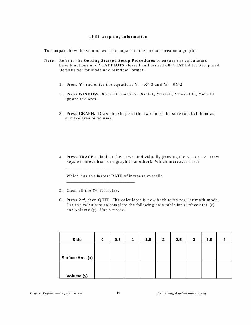
To compare how the volume would compare to the surface area on a graph:
Note: Refer to the Getting Started Setup Procedures to ensure the calculators have functions and STAT PLOTS cleared and turned off, STAT Editor Setup and Defaults set for Mode and Window Format.
1. Press Y= and enter the equations Y1 = X^ 3 and Y2 = 6X^2
2. Press WINDOW. Xmin=0, Xmax=5, Xscl=1, Ymin=0, Ymax=100, Yscl=10. Ignore the Xres.
3. Press GRAPH. Draw the shape of the two lines - be sure to label them as surface area or volume.
4. Press TRACE to look at the curves individually (moving the <--- or --> arrowkeys will move from one graph to another). Which increases first?________________________________
Which has the fastest RATE of increase overall?_________________________________
5. Clear all the Y= formulas.
6. Press 2nd, then QUIT. The calculator is now back to its regular math mode.Use the calculator to complete the following data table for surface area (x)and volume (y). Use s = side.
Side 0 0.5 1 1.5 2 2.5 3 3.5 4
Surface Area (x)
Volume (y)
Virginia Department of Education 20 Connecting Algebra and Biology
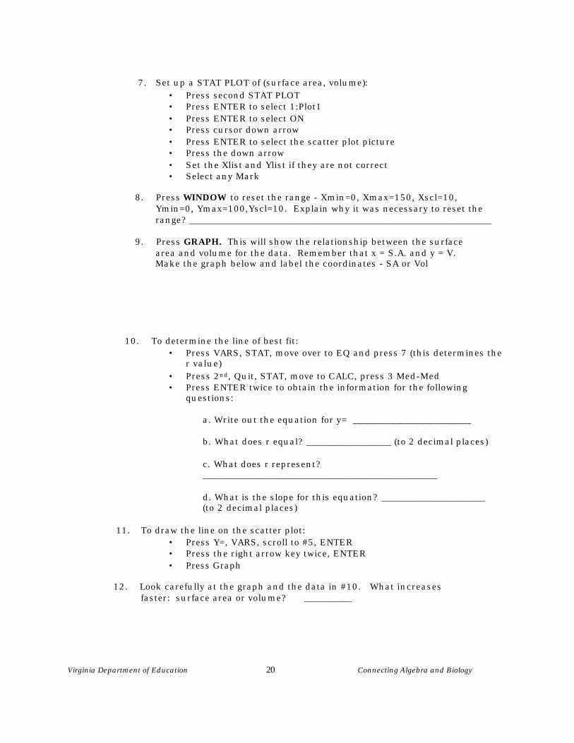
7. Set up a STAT PLOT of (surface area, volume):
• Press second STAT PLOT• Press ENTER to select 1:Plot1• Press ENTER to select ON• Press cursor down arrow• Press ENTER to select the scatter plot picture• Press the down arrow• Set the Xlist and Ylist if they are not correct• Select any Mark
8. Press WINDOW to reset the range - Xmin=0, Xmax=150, Xscl=10, Ymin=0, Ymax=100,Yscl=10. Explain why it was necessary to reset the range? ________________________________________________________________
9. Press GRAPH. This will show the relationship between the surface area and volume for the data. Remember that x = S.A. and y = V.
Make the graph below and label the coordinates - SA or Vol
10. To determine the line of best fit:• Press VARS, STAT, move over to EQ and press 7 (this determines the
r value)
• Press 2nd, Quit, STAT, move to CALC, press 3 Med-Med• Press ENTER twice to obtain the information for the following
questions:
a. Write out the equation for y= _________________________
b. What does r equal? __________________ (to 2 decimal places)
c. What does r represent? __________________________________________________
d. What is the slope for this equation? ______________________(to 2 decimal places)
11. To draw the line on the scatter plot:• Press Y=, VARS, scroll to #5, ENTER• Press the right arrow key twice, ENTER• Press Graph
12. Look carefully at the graph and the data in #10. What increases faster: surface area or volume? __________
Virginia Department of Education 21 Connecting Algebra and Biology
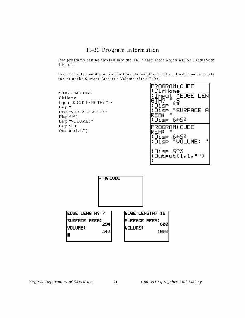
TI-83 Program Information
Two programs can be entered into the TI-83 calculator which will be useful withthis lab.
The first will prompt the user for the side length of a cube. It will then calculateand print the Surface Area and Volume of the Cube.
PROGRAM:CUBE:ClrHome:Input “EDGE LENGTH? “, S:Disp “”:Disp “SURFACE AREA: “:Disp 6*S2
:Disp “VOLUME: “:Disp S^3:Output (1,1,””)

Virginia Department of Education 22 Connecting Algebra and Biology
The second will prompt the user for the Volume of the Cube. It will thencompute and display the Surface Area and the ratio of the Surface Area to theVolume.
PROGRAM:CELL:ClrHome:Input “VOLUME OF CUBE? “,V:ClrHome:Disp “SURFACE AREA = “
:6*3x√V2àS:Disp S:Disp “”:Disp “RATIO SA/V = “:Disp S/V:Output (1,1,””)

Virginia Department of Education 23 Connecting Algebra and Biology
CASIO 9850 G+ Graphing Information
To enter the equations y = x^3 and y = 6x^2 into the graphing calculator:
Go to GRAPH Mode (#5)• Press the X,Θ,Τ key located below the red ALPHA key. Press
the ^ key located beneath the VARS key.
• Press the number 3. Press the EXE key. The formula forvolume of a cube has now been entered.
• Press the number 6. Press the X,Θ,Τ key located below thered ALPHA key. Press the ^ key located beneath the VARSkey.
• Press the number 2. Press the EXE key. The formula forsurface area of a cube has now been entered.
• Press the SHIFT key. Press F3 (V-Window). Set the viewingwindow as follows: Xmin = 0, Xmax = 5, Xscale = 1, Ymin = 0,Ymax = 100, and Yscale = 10. Press the EXIT key.
• Press F6 (DRAW).
1. Describe the shape of the two curves.
2. Which increases faster, the area or the volume?
Complete the following data table for the surface area (x) and volume (y) of acube over the range 0 to 4.5.
Side 0 0.5 1 1.5 2 2.5 3 3.5 4 4.5
Surface Area (x)
Volume (y)
The data table can easily be filled in by putting a program into the RUN Mode (#1) ofthe graphing calculator.

Virginia Department of Education 24 Connecting Algebra and Biology
Extension
1. Enter the ordered pairs (x,y) = (surface area, volume) into a two-variable statisticaldata set within your graphing calculator.
2. Use the graphing calculator to draw a scatter plot in a range of Xmin = 0, Xmax =150, Xscale = 10, Ymin = 0, Ymax = 100, and Yscale = 10.
3. Find the best fitting line for the data points (linear regression). Write the equationbelow.
Y = _________________________ r = _________________________
4. What is the slope of the line?
5. What is the significance of this value?
6. Looking at the data, which increases most rapidly, the volume or the area?

Virginia Department of Education 25 Connecting Algebra and Biology
CASIO 9850 G+ Program Information
Go to RUN Mode (#1).
Press the yellow SHIFT key. Press the VARS key. This is the PRGM screen.
• Press F4 (?). Press the send to arrow key (→) located above theAC/ON key.
• Press the red ALPHA key. Press the multiplication symbol (x).• Press F6 (ω).• Press F5 (:).• Press the red ALPHA key. Press the multiplication symbol (x).• Press the ^ key located below the VARS key.• Press the number 3.• Press F6 (ω).• Press F5 (ψ).• Press the number 6. Press the multiplication symbol (x).• Press the red ALPHA key. Press the multiplication symbol (x).• Press the ^ key located below the VARS key. Press the number 2.• Press the EXE key. At this point there should be a question mark
below the program you have just inputted.
Input each of the side values from the data chart and the program will calculatethe volume first and then the surface area.
• Press the number 0. Press the EXE key.This is the volume for a side of 0.
• Press the EXE key. This is the surface area for a side of 0. Continueputting in each side value in order to complete the data chart.

Virginia Department of Education 26 Connecting Algebra and Biology
Genetics: What is the Chance?
Related SOL: BIO.1, BIO.6, and A.18
OverviewGenetic problems express the probability that a certain event will occur at any one time.The more things that are introduced into the mix, the less likely it becomes that thingswill happen as expected.Back in the 1870's Gregor Mendel, an Austrian monk, noticed patterns between parentsand offspring in the sweetpea, Pisum savium. These patterns occurred with a degree ofregularity. Mendel wondered if these patterns had a mathematical order orpredictability to them. All of the sweetpea traits that Mendel studied were independentor discrete events gene residing on a separate chromosome.This activity also examines what would happen if Mendel had chosen genes that arelinked together (genes that are located on the same chromosome).
Materials four coins
clear plastic tape graphing calculator
Procedure
1. If a coin is tossed fifty times, predict how many times it would landon heads and how many times it would land on tails. Enter the datainto Table #1.
2. Take one of the four coins. Flip it in the air exactly fifty times. Count the number of times it lands on heads and the number on tails. Complete data table #1.
Data Table #1 Heads Tails
Predicted Actual Predicted Actual
3. Take two coins. Flip them at the same time for fifty times. Count thenumber of times they land head-head, tail-tail, or head-tail. Fill indata table #2.
Virginia Department of Education 27 Connecting Algebra and Biology
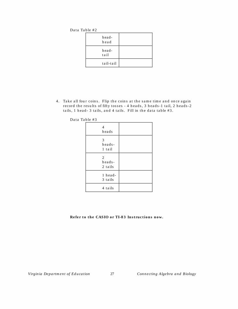
Data Table #2
head-head
head-tail
tail-tail
4. Take all four coins. Flip the coins at the same time and once againrecord the results of fifty tosses - 4 heads, 3 heads-1 tail, 2 heads-2tails, 1 head- 3 tails, and 4 tails. Fill in the data table #3.
Data Table #3
4heads
3heads-1 tail
2heads-2 tails
1 head-3 tails
4 tails
Refer to the CASIO or TI-83 Instructions now.

Virginia Department of Education 28 Connecting Algebra and Biology
Analysis
1. What was the ratio found in the first experiment? Remember to reduce to lowest possible numbers. PREDICTED RATIO _______TO________
ACTUAL RATIO _______TO________
2. What was the ratio found in the second experiment? TO TO
3. Express the ratio of the third experiment in terms of whole numbers but in smallestpossible numbers. TO TO TO TO
4. Were any parts of experiment three’s ratio similar or very close? Explain the answer.
5. Compare/contrast the 3 graphs.
Data chart #1 Data chart #2
Data chart #3
5. Would very different ratios be expected if this experiment were done 200 times? Why or why not? Which set of tosses would be more accurate?

Virginia Department of Education 29 Connecting Algebra and Biology
CASIO 9850 G+ Graphing Information
Steps for Data Chart 1:
• Press MENU. Go to STAT (#2) icon and press EXETo avoid confusion, enter the tails information with the 1 and the
heads information with the 2.
• In List1, enter 1 and 2. In List2 enter the number of tails and then thenumber of heads from Data Chart 1.
• Press F1(GRPH) to graph the information
• Press F6(SET) to set up the graph
Graph Type: F6, F1(Hist) Xlist: F1(List1) Frequency: F3(List2) Mark Type: Any of the choices Graph Color: Any of the choices
• Press EXIT, F4(SEL). Make sure that StaGraph1 is On and the rest are Off.
• Press F6. Highlight pitch and change it to .25. Press EXE.
• Press F6 for DRAW.
Steps for Data Chart 2:
• Repeat the steps for Data Chart 1 except
In List1 enter 1 for 2 tails; 2 for 2 heads; 3 for 1 head-1 tail.
Steps for Data Chart 3:
• Repeat the steps for Data Chart 1 except
In List1 enter 1 for 4 tails; 2 for 4 heads; 3 for 3 heads-1 tail; 4 for 2heads-2 tails; 5 for 1 head-3 tails.

Virginia Department of Education 30 Connecting Algebra and Biology
TI-83 Graphing Information
Note: Refer to the Getting Started Setup Procedures to set up yourCalculator with the unwanted functions and STAT PLOTS turned off,Lists cleared, proper MODE settings, etc.
Steps for Data Chart 1
Use List1 as the list for heads or tails.
Use List2 as the list for number of occurrences as entered in the datachart.
• Press STAT• Select 1: EDIT• Clear List1 and List2• Enter 1 for heads and 2 for tails into List1• Enter the number of heads opposite the 1 and the number of tails
opposite the 2 into List2
WINDOW Settings:
• Press WINDOW• Enter Xmin = 0, Xmax = 3, xscl = 1, Ymin = -1, Ymax = 50, Yscl = 5
To Graph
• Press 2nd STAT PLOT• Press ENTER to select Plot1• Press ENTER to turn on Plot1• Press the down arrow key to move the cursor to TYPE• Press the right arrow key to the 3rd icon for Histogram• Press ENTER to highlight Histogram.• Press the down arrow key to move the cursor to Xlist The Xlist should be L1. NOTE: L1 is a 2nd function over the 1 key.• Press the down arrow key to Freq
The Freq should be L2.
NOTE: L2 is the 2nd function over the 2 key.
• Press GRAPH to view the histogram• Press TRACE to trace on the histogram
The min and max values for each bar as well as the number of entries in that range are given.
Virginia Department of Education 31 Connecting Algebra and Biology
Steps for Data Chart 2
Repeat the process for Data Chart 1 with these changes:• Enter into List1, 1 to represent 2 heads; 2 to represent 1 head-1 tail; 3 to represent 2 tails
WINDOW Setting:
• Change Xmax to 4
Steps for Data Chart 3
Repeat the process for Data Chart 1 with these changes:
• Enter into List 1, 1 to represent 4 heads; 2 to represent 3 heads-1 tail; 3 to represent 2 heads- 2 tails;
4 to represent 1 head- 3 tails; 5 to represent 4 tails
WINDOW Setting
• Change Xmax to 6
Virginia Department of Education 32 Connecting Algebra and Biology
WEIGHTS AND DRUG DOSES
Related SOL: BIO. 1, BIO.2, BIO.4, BIO.5, and A.17
OverviewEvery day in the newspaper, one can read about bacteria – how theycause disease, how they are used in research, and how they are
becoming resistant to our medicines. These tiny prokaryotic cellsare important to all life in many different ways.
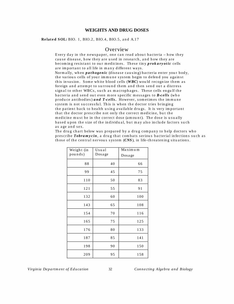
Normally, when pathogenic (disease causing) bacteria enter your body,the various cells of your immune system begin to defend you againstthis invasion. Some white blood cells (WBC) would recognize them asforeign and attempt to surround them and then send out a distresssignal to other WBCs, such as macrophages. These cells engulf thebacteria and send out even more specific messages to B-cells (whoproduce antibodies) and T-cells. However, sometimes the immunesystem is not successful. This is when the doctor tries bringingthe patient back to health using available drugs. It is very importantthat the doctor prescribe not only the correct medicine, but themedicine must be in the correct dose (amount). The dose is usuallybased upon the size of the individual, but may also include factors suchas age and sex.The drug chart below was prepared by a drug company to help doctors whoprescribe Tobramycin, a drug that combats serious bacterial infections such asthose of the central nervous system (CNS), in life-threatening situations.
Weight (inpounds)
UsualDosage
Maximum
Dosage
88 40 66
99 45 75
110 50 83
121 55 91
132 60 100
143 65 108
154 70 116
165 75 125
176 80 133
187 85 141
198 90 150
209 95 158
Virginia Department of Education 33 Connecting Algebra and Biology
Procedure
Refer to the CASIO or TI information now.
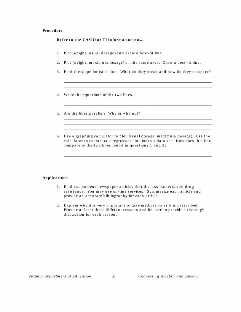
1. Plot (weight, usual dosage) and draw a best-fit line.
2. Plot (weight, maximum dosage) on the same axes. Draw a best-fit line.
3. Find the slope for each line. What do they mean and how do they compare?_________________________________________________________________________________________________________________________________________________________________________________________________________________________________
4. Write the equations of the two lines.______________________________________________________________________________________________________________________________________________________
5. Are the lines parallel? Why or why not?___________________________________________________________________________
_____________________________________________________________________________________________________________________________________________________
6. Use a graphing calculator to plot {usual dosage, maximum dosage}. Use thecalculator to construct a regression line for this data set. How does this linecompare to the two lines found in questions 1 and 2?
_____________________________________________________________________________________________________________________________________________________________________________________________
Applications
1. Find two current newspaper articles that discuss bacteria and drugresistance. You may use on-line services. Summarize each article andprovide an accurate bibliography for each article.
2. Explain why it is very important to take medication as it is prescribed.Provide at least three different reasons and be sure to provide a thoroughdiscussion for each reason.

Virginia Department of Education 34 Connecting Algebra and Biology
CASIO 9850 G+ Graphing Information
• Go to STAT Mode (#2). Enter the weight into List 1, the usual dosage into List 2,and the maximum dosage into List 3.
• Select F1 (GRPH). Select F6 (SET). Use the down arrow key to highlight Graph Type,and press F1 (Scat). Arrow down to highlight XList, and press F1 (List 1). Arrowdown to highlight YList, and press F2 (List 2). Arrow down to highlight Frequency,and press F1 (1). For the settings Mark Type and Graph Color, make your ownchoices. Press the EXIT key.
• Select F6 (SET). This time select F2 (GPH2). Use the down arrow key to highlightGraph Type, and press F1 (Scat). Arrow down to highlight XList, and press F1 (List1). Arrow down to YList, and press F3 (List 3). Arrow down to highlight Frequency,and press F1 (1). For the settings Mark Type and Graph Color, make your ownchoices. Press the EXIT key.
• Select F4 (SEL). StatGraph1 should be highlighted. Make sure it says, “DrawOn”next to it. If not, press F1 (On). Make sure that StatGraph2 and StatGraph3 say,“DrawOff” next to them. If not, press F2 (Off). Press F6 (DRAW).
• Press the EXIT key. Select F4 (SEL). To graph only StatGraph2, when StatGraph1 ishighlighted, press F2 (Off). Arrow down to highlight StatGraph2, press F1 (On).Press F6 (DRAW).
• To answer question 6, press the EXIT key. Press F6 (SET), and then F3 (GPH3). Setthe Graph Type to Scatter, the XList to List 2, the YList to List 3, and the Frequencyto 1. Press the EXIT key. Select F4 (SEL). Make sure that only StatGraph3 isturned on. Press F6 (DRAW). When the graph appears, select F2 for the Median-Median line information. Press F6 (DRAW) to draw the line on the scatter plot.

Virginia Department of Education 35 Connecting Algebra and Biology
TI-83 Graphing Information
Note: Refer to the Getting Started Setup Procedures to ensure the calculators havefunctions and STAT PLOTS cleared or turned off, STAT Editor Setup and Defaults setfor Mode and Window Format.
Data Entry
Enter the information from your data table into the lists.Use L1 for the Weight (pounds)Use L2 for the Usual dosage (mg)Use L3 for the Maximum dosage (mg)
1. Press STAT Select 1:Edit
2. Key the values from the activity sheet into the lists.
Scatter Plots
Activity Sheet Question #1 Plot (weight, usual dosage)
Weight is the independent variable so L1 (weight) will be the Xlist.Usual dosage is the dependent variable so L2 (usual dosage) will be the Ylist.
Set up a STAT PLOT
• Press 2nd STAT PLOT • Press ENTER to select 1:Plot1
• Press ENTER to select ON • Press cursor down arrow • Press ENTER to select the scatter plot picture.
• Press the down arrow • Set the Xlist and Ylist if they are not correct. Press 2nd L1 (this is the number 1 key) • Select a Mark. Generally the box or + are best if there are not a lot of data points. The dot is best if there are a large number of data points.
Virginia Department of Education 36 Connecting Algebra and Biology
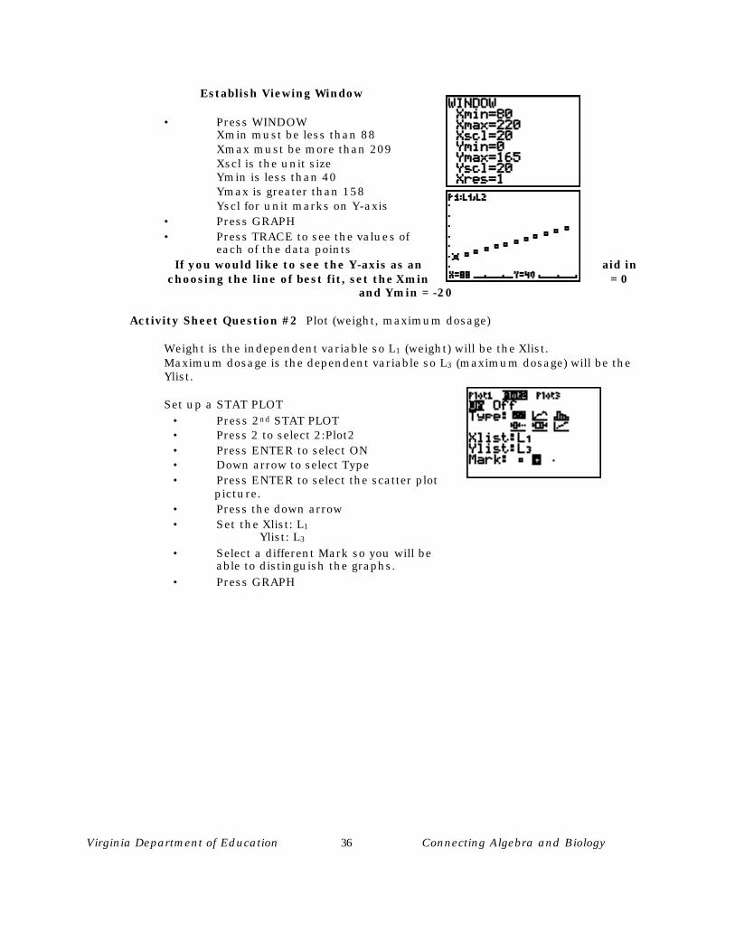
Establish Viewing Window
• Press WINDOW Xmin must be less than 88 Xmax must be more than 209 Xscl is the unit size Ymin is less than 40 Ymax is greater than 158 Yscl for unit marks on Y-axis
• Press GRAPH• Press TRACE to see the values of
each of the data pointsIf you would like to see the Y-axis as an aid in
choosing the line of best fit, set the Xmin = 0and Ymin = -20
Activity Sheet Question #2 Plot (weight, maximum dosage)
Weight is the independent variable so L1 (weight) will be the Xlist.Maximum dosage is the dependent variable so L3 (maximum dosage) will be theYlist.
Set up a STAT PLOT
• Press 2nd STAT PLOT • Press 2 to select 2:Plot2 • Press ENTER to select ON • Down arrow to select Type • Press ENTER to select the scatter plot picture. • Press the down arrow • Set the Xlist: L1
Ylist: L3
• Select a different Mark so you will be able to distinguish the graphs.
• Press GRAPH

Virginia Department of Education 37 Connecting Algebra and Biology
Activity Sheet Question #6 Plot (usual dosage, maximum dosage)
Turn off the previous Plots• Press 2nd STAT PLOT• Press 4: PlotsOff
This will paste the command to the home screen
• Press ENTER to execute the command
• Press 2nd STAT PLOT to return to the STAT PLOT menu
• Select 3:Plot3 In this way the other Plots remain available • Set it up as shown.
• Set the Xlist: L2 ;Ylist: L3
• Fix the WINDOW for a different Xlist
• Press GRAPH
Virginia Department of Education 38 Connecting Algebra and Biology
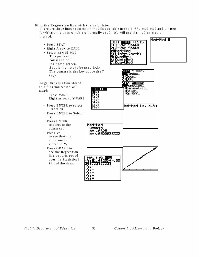
Find the Regression line with the calculatorThere are three linear regression models available in the TI-83. Med-Med and LinReg(ax+b) are the ones which are normally used. We will use the median-medianmethod.
• Press STAT• Right Arrow to CALC• Select #3Med-Med
This pastes thecommand onthe home screen.
Supply the lists to be used L2,L3
(The comma is the key above the 7 key)
To get the equation stored as a function which will graph
• Press VARS Right arrow to Y-VARS
• Press ENTER to selectFunction
• Press ENTER to SelectY1
• Press ENTER to execute the command
• Press Y= to see that the
equation is stored in Y1
• Press GRAPH to see the Regression line superimposed over the Statistical Plot of the data.

Virginia Department of Education 39 Connecting Algebra and Biology
• MODE G-T allows youto view the graph andTable
• Press TRACE to traceon the STAT PLOT
• Press down arrow forthe TRACE to move to
the equation.
Virginia Department of Education 40 Connecting Algebra and Biology
You Gotta Have Heart
Related SOL: BIO.1, BIO.5, and A.18
Overview What do you know about your heartbeat? All organisms with a closed circulatory system have a pump to move the blood and therefore have a heartbeat. Various drugs affect the heart - some speed up the heart rate (stimulants) and others slow the heart rate (depressants). In this laboratory exercise, you will test the effect of a common drug – caffeine. The class will test a variety of common everyday beverages and food that contain caffeine.
Materials one can 12 oz of soda, diet caffeine free one can 12 oz of soda, diet with caffeine (Mountain Dew has a lot of caffeine) 12 oz of coffee - caffeinated 12 oz of tea - not herbal one chocolate candy bar, no nuts clock with second hand
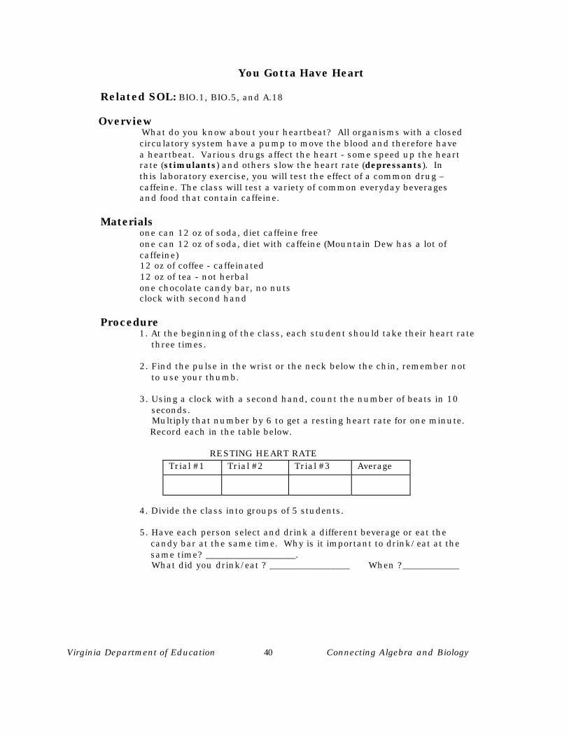
Procedure 1. At the beginning of the class, each student should take their heart rate three times.
2. Find the pulse in the wrist or the neck below the chin, remember not to use your thumb.
3. Using a clock with a second hand, count the number of beats in 10 seconds.
Multiply that number by 6 to get a resting heart rate for one minute. Record each in the table below.
RESTING HEART RATE
Trial #1 Trial #2 Trial #3 Average
4. Divide the class into groups of 5 students.
5. Have each person select and drink a different beverage or eat the candy bar at the same time. Why is it important to drink/eat at the same time? ___________________. What did you drink/eat ? _________________ When ?____________
Virginia Department of Education 41 Connecting Algebra and Biology
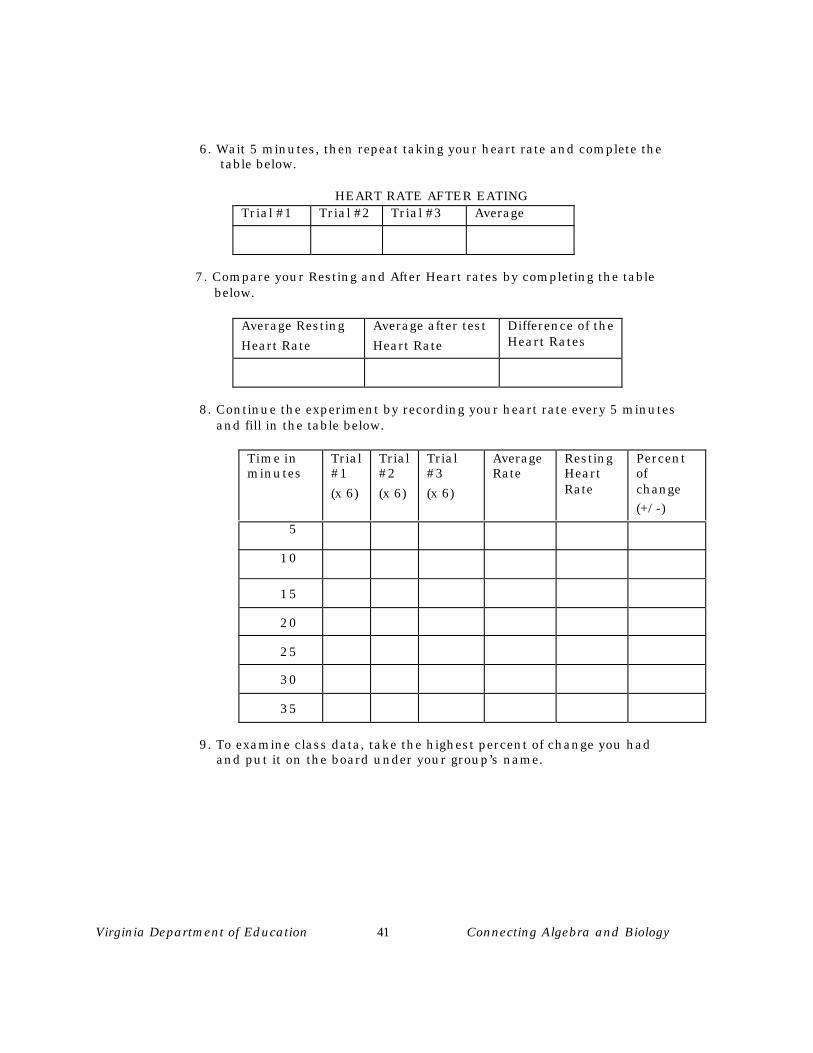
6. Wait 5 minutes, then repeat taking your heart rate and complete the table below.
HEART RATE AFTER EATINGTrial #1 Trial #2 Trial #3 Average
7. Compare your Resting and After Heart rates by completing the table below.
Average Resting
Heart Rate
Average after test
Heart Rate
Difference of theHeart Rates
8. Continue the experiment by recording your heart rate every 5 minutes and fill in the table below.
Time inminutes
Trial#1
(x 6)
Trial#2
(x 6)
Trial#3
(x 6)
AverageRate
RestingHeartRate
Percentofchange
(+/-)
5
10
15
20
25
30
35
9. To examine class data, take the highest percent of change you had and put it on the board under your group’s name.

Virginia Department of Education 42 Connecting Algebra and Biology
10. Fill in the table below from the board and find the average rate of increase for the substance tested.
CLASS DATA TABLESubstanceTested (X)
Group 1 Group 2 Group 3 Group 4 Group 5 Group 6
Decaf Soda
(X=1)
RegularSoda
(X=2)
Coffee
(X=3)
Tea
(X=4)
Chocolate
(X-5)
Graphing: Refer to the CASIO or TI instructions.
Virginia Department of Education 43 Connecting Algebra and Biology
Analysis and Conclusions
1. Was caffeine a stimulant or a depressant? ____________________
2. What was your proof for this answer?
3. What were the constants in this experiment?
4. What was the dependent variable in this experiment? ____________________
5. What was the reason for using diet beverages?
6. Which substance had the greatest effect on the heart rate? _________________
7. Which group had the greatest increase in heart rate? ______________________
8. What might be other contributing factors that could have altered the results of this experiment?
9. How might you change this experiment to remove these factors or keep them constant?
Virginia Department of Education 44 Connecting Algebra and Biology
CASIO 9850 G+ Graphing Instructions
1. Using the data make a histogram showing the heart rate increase (using averages) for each substance. (For example, if the average heart rate increase for decaf. soda was 8, then enter a 1 for x and 8 for y. If the average heart rate increase for soda was 5, then you enter 2 for x and 5 for y. Continue entering the data for coffee (x=3, y=average), tea (x=4, y=average), and chocolate (x=5, y=average). Set the viewing window to the following specifications: Xmin = .5, Xmax = number of groups in class + .5, Xscale = 1, Ymin = 0, Ymax = 15, and Yscale = 5.
Go to STAT Mode (#2). Make sure to clear out any existing lists.
• Enter in the new data by putting the x-axis values into List 1, and y-axis values into List 2.
• Press F1 (GRPH), and then F6 (SET).• Arrow down to highlight Graph Type. Press F6 (ω). Press F1 (Hist).• Arrow down to highlight XList. Press F1 (List 1).• Arrow down to highlight Frequency. Press F3 (List 2).• Choose any graph color you want. Press the EXIT key.
At this point, set the viewing window to the correct specifications.• Press the yellow SHIFT key, followed by the F3 (V-Window) key.• The Xmin should already be highlighted. Change it to .5, then press
the EXE key.• Xmax should now be highlighted. Change it to the number of five-
person groups in the class + .5, then press the EXE key.• Xscale should now be highlighted. Change it to 1, and then press the
EXE key.• Ymin should now be highlighted. Change it to 0, and then press the
EXE key.• Ymax should now be highlighted. Change it to 15, and then press
the EXE key.
• Yscale should now be highlighted. Change it to 5, and then press theEXE key.
• Press the EXE key again.• Press F1 (GRPH).• Press F4 (SEL). Make sure the only graph that is on is StatGraph1.
• Press F6 (DRAW). This is the Set Interval window.• Set the Start at 1. Press the EXE key. Set the pitch at 1. Press the
EXE key. Press F6 (DRAW).

Virginia Department of Education 45 Connecting Algebra and Biology
2. Make a histogram choosing one of the 5 substances and using all groups in the class for that substance. (Let x=1 for group 1, and y=average heart rate for group 1. Let x=2 for group 2, and y=average heart rate for group 2. Continue
inputting data until each group’s data has been included.) Set the viewing window as follows: Xmin = .5, Xmax = number of groups + .5, Xscale = 1, Ymin = 0, Ymax = 30, and Yscale = 5.
Virginia Department of Education 46 Connecting Algebra and Biology
TI-83 Graphing Information
Note: Refer to the Getting Started Setup Procedures to ensure the calculators have functions and STAT PLOTS cleared or turned off, STAT Editor Setup and Defaults set for Mode and Window Format.
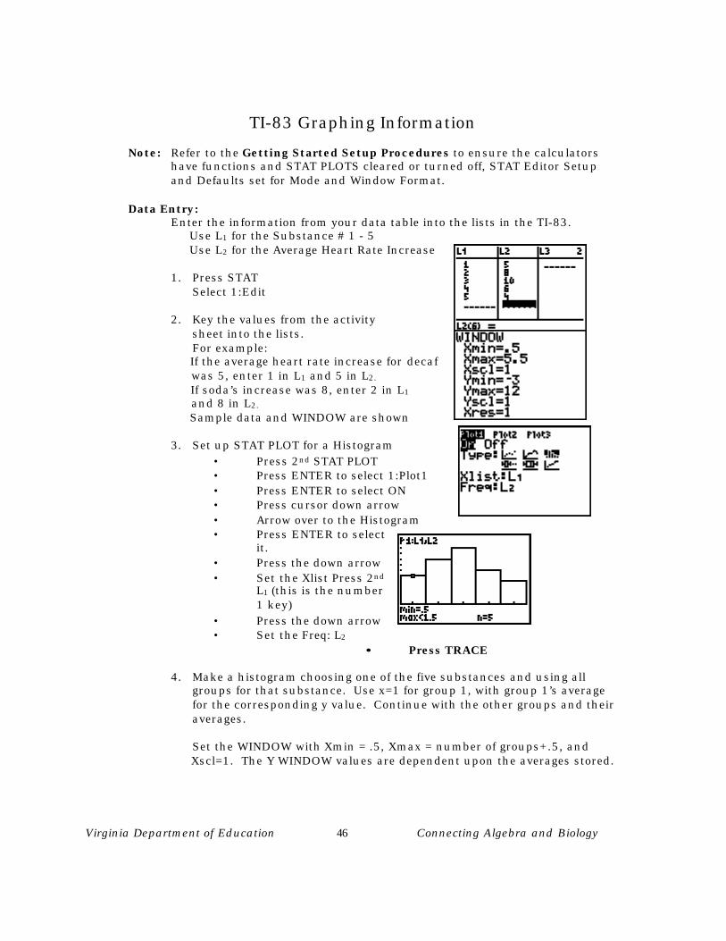
Data Entry: Enter the information from your data table into the lists in the TI-83.
Use L1 for the Substance # 1 - 5 Use L2 for the Average Heart Rate Increase
1. Press STATSelect 1:Edit
2. Key the values from the activitysheet into the lists.For example:
If the average heart rate increase for decaf was 5, enter 1 in L1 and 5 in L2.
If soda’s increase was 8, enter 2 in L1
and 8 in L2.
Sample data and WINDOW are shown
3. Set up STAT PLOT for a Histogram
• Press 2nd STAT PLOT • Press ENTER to select 1:Plot1 • Press ENTER to select ON • Press cursor down arrow • Arrow over to the Histogram • Press ENTER to select
it. • Press the down arrow • Set the Xlist Press 2nd
L1 (this is the number1 key)
• Press the down arrow • Set the Freq: L2
•• Press TRACE
4. Make a histogram choosing one of the five substances and using allgroups for that substance. Use x=1 for group 1, with group 1’s averagefor the corresponding y value. Continue with the other groups and theiraverages.
Set the WINDOW with Xmin = .5, Xmax = number of groups+.5, and Xscl=1. The Y WINDOW values are dependent upon the averages stored.

Virginia Department of Education 47 Connecting Algebra and Biology
The Hermit’s Epidemic
Related SOL: BIO.1, BIO.5, and A.18
Overview Six (unusually sociable) hermits live on an otherwise deserted island. An infectious disease strikes the island. The disease has a one-day infectious period and after that the person is immune (cannot get the disease again). Assume one of the hermits gets the disease (maybe from a piece of Skylab). He randomly visits one of the other hermits during his infectious period. If the visited hermit has not had the disease, he gets it and is infectious the following day. The visited hermit then visits another hermit. The disease is transmitted until an infectious hermit visits another hermit. The disease is transmitted until an infectious hermit visits an immune hermit, and the disease dies out. There is one hermit visit per day. Assuming this pattern of behavior, how many hermits can be expected, on the average, to get the disease?
Pre- Activity Questions
1. What is the least number of hermits that could get infected?
2. What is the greatest number of hermits that could get infected?
3. What sort of model could you use for this problem?
4. How would you solve this problem analytically?
5. How would changing the number of hermits on the island affect the expectednumber of infected hermits?
Procedure
1. Use a six-sided die where each side represents a hermit.
2. Roll the die to see which hermit gets the disease.
3. Roll the die again to see which hermit is visited and gets the disease.
4. Continue rolling until an immune hermit (one of the numbers that has already been rolled) is visited. NOTE: If the same number is rolled one after the other, ignore the second roll, since these hermits do not visit themselves.
5. Count how many different numbers were rolled (how many hermits got thedisease).

Virginia Department of Education 48 Connecting Algebra and Biology
6. Repeat steps 2 through 5 ten times.
Refer to the CASIO or TI-83 Information for an alternate method.
Virginia Department of Education 49 Connecting Algebra and Biology
CASIO CFX-9850 G+ Information
Method I:
• Go to the RUN Mode (#1).• Press the yellow SHIFT key, and then
the MENU key This will get into the SET UP.
• Arrow down to “Display” Press F1 (Fix). Press F1 (0) Press the EXIT key• Press the OPTN key. Press F6 (ω). Press F3 (PROB)• Type in the maximum random number minus one. For example, in this
simulation of rolling a die to utilize the numbers 1 through 6 (random number,6, minus 1).
• Press F4 (Ran#).• Press the addition symbol (+). Press the number 1. Hit the EXE key repeatedly
to produce as many random numbers as needed.
Method II:
• Go to the RUN Mode (#1).• Press the OPTN key. Press F6 (ω). Press
F4 (NUM). Press F2 (Int).Type in the maximum random number (6 in this case).
• Press the EXIT key.• Press F3 (PROB). Press F4 (Ran#).• Press the addition symbol (+), followed by the number 1.• Press the yellow SHIFT key. Press the MENU key. To go into SET UP.• Arrow down to “Display”. Press F1 (Fix). Press F1 (0). Press the EXIT key. Hit
the EXE key repeatedly to produce as many random numbers as needed.
Virginia Department of Education 50 Connecting Algebra and Biology
TI-83 Information
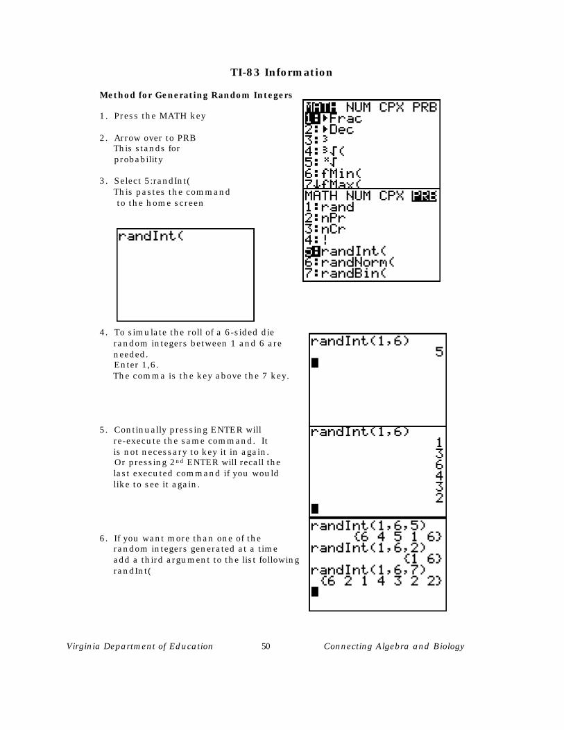
Method for Generating Random Integers
1. Press the MATH key
2. Arrow over to PRB This stands for probability
3. Select 5:randInt( This pastes the command to the home screen
4. To simulate the roll of a 6-sided die random integers between 1 and 6 are needed. Enter 1,6. The comma is the key above the 7 key.
5. Continually pressing ENTER will re-execute the same command. It is not necessary to key it in again. Or pressing 2nd ENTER will recall the last executed command if you would like to see it again.
6. If you want more than one of the random integers generated at a time add a third argument to the list following randInt(
Virginia Department of Education 51 Connecting Algebra and Biology
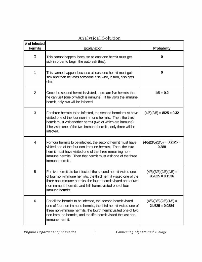
Analytical Solution# of Infected
Hermits Explanation Probability
0 This cannot happen, because at least one hermit must get 0sick in order to begin the outbreak (trial).
1 This cannot happen, because at least one hermit must get 0sick and then he visits someone else who, in turn, also getssick.
2 Once the second hermit is visited, there are five hermits that 1/5 = 0.2he can visit (one of which is immune). If he visits the immunehermit, only two will be infected.
3 For three hermits to be infected, the second hermit must have (4/5)(2/5) = 8/25 = 0.32visited one of the four non-immune hermits. Then, the thirdhermit must visit another hermit (two of which are immune).If he visits one of the two immune hermits, only three will beinfected.
4 For four hermits to be infected, the second hermit must have (4/5)(3/5)(3/5) = 36/125 =visited one of the four non-immune hermits. Then, the third 0.288hermit must have visited one of the three remaining non-immune hermits. Then that hermit must visit one of the threeimmune hermits.
5 For five hermits to be infected, the second hermit visited one (4/5)(3/5)(2/5)(4/5) =of four non-immune hermits, the third hermit visited one of the 96/625 = 0.1536three non-immune hermits, the fourth hermit visited one of twonon-immune hermits, and fifth hermit visited one of fourimmune hermits.
6 For all the hermits to be infected, the second hermit visited (4/5)(3/5)(2/5)(1/5) =one of four non-immune hermits, the third hermit visited one of 24/625 = 0.0384three non-immune hermits, the fourth hermit visited one of twonon-immune hermits, and the fifth hermit visited the last non-immune hermit.
Virginia Department of Education 52 Connecting Algebra and Biology
In order to solve this problem analytically, you must find the probability that eachpossible number of hermits will be infected. There will be at least two infected (one getsthe disease and visits another) and at most six infected (all get visited without anyonegetting visited twice). Look at each case separately.
Now we can find the expected value, E(x), by multiplying each value by its respectiveprobability and adding them all together.
E(x) = 0(0) + 1(0) + 2(1/5) + 3(8/25) + 4(36/125) + 5(96/625) + 6(24/625) =
0 + 0 + (2/5) + (24/25) + (144/125) + (480/625) + (144/625) =
(250/625) + (600/625) + (720/625) + (480/625) + (144/625) =
(2194/625) = 3.5104
Thus, by averaging all the trials from the model, you should get something near 3.5104as your answer.
Questions
1. Should the average of the trials from the model be exactly 3.5104?
2. Does an expected value of 3.5104 mean that we expect 3 whole hermits and onlypart of a fourth hermit to get sick each time?
3. How accurate are the answers from the models?
Extension
1. How could you model an island with 4 hermits? 10 hermits? 52 hermits?
2. What would the expected value of this problem be if there were 4 hermits?10 hermits?
Virginia Department of Education 53 Connecting Algebra and Biology
What’s The Change?
Related SOL: BIO.1, BIO.3, and A.17
OverviewMany textbooks teach that the rate of chemical change doubles for each10° C change in temperature. Although this is a good generalization,temperature does not affect all chemical changes the same, and the rateof increase of a chemical change with respect to temperature is anindividual thing for each different change.In the following reaction between Effervescent Aspirin Tablets and water,the rate of reaction is generally affected by the temperature of the water.The increase is exponential and can be graphed, but it will give less than
a doubling per each 10° C rise in temperature.
Materials
5 Effervescent Aspirin TabletsData Collector and Temperature ProbeIce or very cold waterRoom temperature waterBoiling or very hot water5 clear plastic cups or 5 250 mL beakersClock or watch (with a second hand)
Procedure
1. Place 150 mL of ice cold water (no ice) in one beaker, 150 mL of room temperaturewater in another beaker, and 150 mL of very hot water in another beaker.
2. Measure and record the temperature of the water in each container.
• Connect the graphing calculator to the Data Analyzer with a data link.• Attach temperature probe to Data Analyzer in CH1.• To operate the Data Analyzer manually, use the following keystrokes:
• Press the ON/OFF key. Press the SHIFT key, followed by the MODEkey to access the SETUP.
• Press the DataLOG key until 5.00 sec. appears on the screen. This isthe number of seconds between each sample taken.
• Press the TRIGGER key.• Press the DataLOG key until 20 appears on the screen. This is the
total number of samples to be taken. Press the TRIGGER key.
• Press the DataLOG key until 1 appears on the screen. This sets theanalyzer to record actual time. Press the TRIGGER key.
Virginia Department of Education 54 Connecting Algebra and Biology
• “Ready” should appear on the left side of the screen. To beginsampling data, press the TRIGGER key.
• When all samples have been taken, “Done” will appear on the screen.• To transfer the data from the Data Analyzer to the graphing calculator.
• Turn the graphing calculator ON. Go to the RUN Mode (#1).• Press the yellow SHIFT key, then the VARS key. This takes us into
the PRGM screen. Press F6 (ω). Press F4 (I/O). Press F4 (Recv). Theword “Receive” should now be on the screen.
• Press the OPTN key. Press F1 (LIST). Press F1 (List). Press thenumber 1. Press the end parenthesis key “)”.
• Press the EXE key. The calculator screen should now say, “DONE”.The time data has now been recorded into List 1.
• We now must input the temperature data into List 2. Press theyellow SHIFT key, then the VARS key. Press F6 (ω). Press F4 (I/O).Press F4 (Recv). Press OPTN. Press F1 (LIST). Press F1 (List). Pressthe number 2. Press the end parenthesis key “)”. Press the EXE key.
• Repeat the above keystrokes on the Data Analyzer to record thetemperature of each of the other beakers of water. Make sure youtransfer the data into Lists 3, 4, 5, and 6.
3. Have a timekeeper give a signal and drop an Effervescent Aspirin Tablet into eachbeaker all at the same time.
4. Record the time in seconds when the Effervescent Aspirin Tablet is completelydissolved (has stopped fizzing).

Virginia Department of Education 55 Connecting Algebra and Biology
5. Fill in the table below with the data you have collected:
Temperature (x) Time (y) Reaction Rate (time/sec.)
• To find the average temperature of each beaker that we sampled with theData Analyzer, we must study Lists 2, 4, and 6 in the graphing calculator.
• Go to RUN Mode (#1). Press OPTN key. Press F1 (LIST). Press F6(ω). Press F6 (ω). Press F1 (Sum). Press the EXIT key. Press F1(LIST). Press F1 (List). Press the number 2. Press the divisionsymbol key (¤). Press F3 (Dim). Press F1 (List). Press the number 2.Press the EXE key. The average temperature put into List 2 is nowon the screen.
• Repeat the above steps to get the average temperature in Lists 4 and6. Record the data in the table provided.
Virginia Department of Education 56 Connecting Algebra and Biology
Extension
1. Enter the data into a two-variable statistical data set within your graphingcalculator where temperature is the x and time is the y.
2. Draw a scatter plot for the data points in the range : Xmin = 0, Xmax = 100, Xscale= 10, Ymin = 0, Ymax = set this number a bit higher than the data you havecollected, and Yscale = 5.
3. Find the best fitting curve for the data.
4. Graph this curve and use the graphing calculator’s trace feature to predict theamount of time necessary for the reaction to be completed in water that is at atemperature about half-way between the hot and room temperature and half-waybetween the cold and room temperature.
5. In another beaker, mix 75 mL of the room temperature water with 75 mL of the coldwater and in another beaker, mix 75 mL of the room temperature water with 75 mLof the hot water.
6. Time and run the reaction, then add this information to the data table provided.
7. How close was this value to your predicted value?% error = ((predicted – measured) ¤ predicted) x 100

Virginia Department of Education 57 Connecting Algebra and Biology
TI-83 Information
Note: Refer to the Getting Started Setup Procedures to ensure the calculators havefunctions and STAT Plots cleared or turned off, STAT Editor Setup and Defaultsset for Mode and Window Format.
Data Entry
1. Enter the information from your data table into the lists in the TI-83.L1 will hold the temperature values (x).L2 will hold the time values (y).
• Go to the STATEditor
1. Press STAT 2. Select
1:Edit
• Key in the values from your data table on the lab sheet
2. Set up a STAT PLOT for reaction rate.• This will be a scatter plot of (temperature, time)
Make Xlist: L1
Ylist: L2
• Press 2nd STAT PLOT• Press ENTER to select 1:Plot1
• Press ENTER to selectON
• Press cursor down arrow
Press ENTER to select the scatter plot picture.
• Press the down arrow• Set the Xlist and Ylist if they are not correct. Press 2nd L1 (this is the number 1 key)
• Select whichever Mark you prefer. Generally the boxor + are best if there are not a lot of datapoints. The dot is best if there are a large number of data points.

Virginia Department of Education 58 Connecting Algebra and Biology
3. Establish a viewing window for the graph.• Press WINDOW key
The x values represent temperature in C°.Set the min and max values accordingly.
Use: Xmin = 0Xmax= 100Xscl = 10
The y values represent time in seconds for the fizzing to stop. Choose Ymax larger than the greatest time.
Use: Ymin = 0Yscl = 5
• Press GRAPH4. Return to the activity sheet for data interpretation.
5. Have the calculator find the Regression Equation which best models the timerequired for the reaction at a given temperature.Since the reaction rate is exponential and predicted to be about doublefor each 10°C rise in temperature, the time required for the tablet tofinish fizzing should be about halved for each 10°C change in temperature.This will still be an exponential regressionmodel.
The calculator can find an exponential regression model for you.
• Press STAT• Right arrow to CALC• Arrow down to ExpReg• Press ENTER (or press 0)
The calculator screen shown is ready to store the equation in Y1.
• Press 2nd L1 (over 1) Press the comma key
• Press 2nd L2
• Press the comma key• Press VARS
• Press right arrow to Y-VARS• Select Function Y1 Press ENTER
The calculator screen is set.
ACTIVITY 1
Virginia Department of Education 59 Connecting Algebra and Biology
FLAPPING GILLS
Related SOL: BIO .1, BIO.5, AND A.17
ObjectiveThe student will investigate how temperature affects the breathing rate of agoldfish.
OverviewWhat happens to the breathing rate as the body temperature increases? The body is able to adjust to the environment in order to maintain HOMEOSTASIS (tendency to maintain internal stability by responding and compensating for environmental changes). What about a fish, would it be able to maintain HOMEOSTASIS? In order to survive all living things must be able to respond to their environment. This laboratory deals with observing how a goldfish=s respiration rate responds to temperature variation in its habitat. What is the independent variable? What is the dependent variable?
Materials
100 ml beaker500 ml tap water at room temperature (leave out over night to remove chlorine)Dishpan with iceGoldfishStopwatchElectronic data collector with temperature probeGraphing calculator
Procedure
1. Pour 500 ml of tap water into a 1000 ml beaker.2. Place the temperature probe into the water and record water temperature.3. Place the goldfish in the beaker of tap water. Allow 5 minutes for the goldfish to stabilize.
Insert temperature probe into the water.4. Set the electronic data collector to record temperature for manual
intervals.5. Using the stopwatch, count the numbe r of gill flaps of the goldfish for
twelve 15-second intervals. At the end of each time interval, record thenumber of gill flaps and activate the temperature recorder.
6. Place the beaker containing the goldfish and temperature probe in thedish pan with ice.Be sure the ice covers the sides of the beaker.
7. Count the gill flaps in 15-second intervals for 10 minutes. Record gillflap counts and temperature at the end of each 15-second interval.
8. Enter data from the data collector and data tables into the graphingcalculator.
9. Using the data, construct graphs comparing temperature and breathingrates.
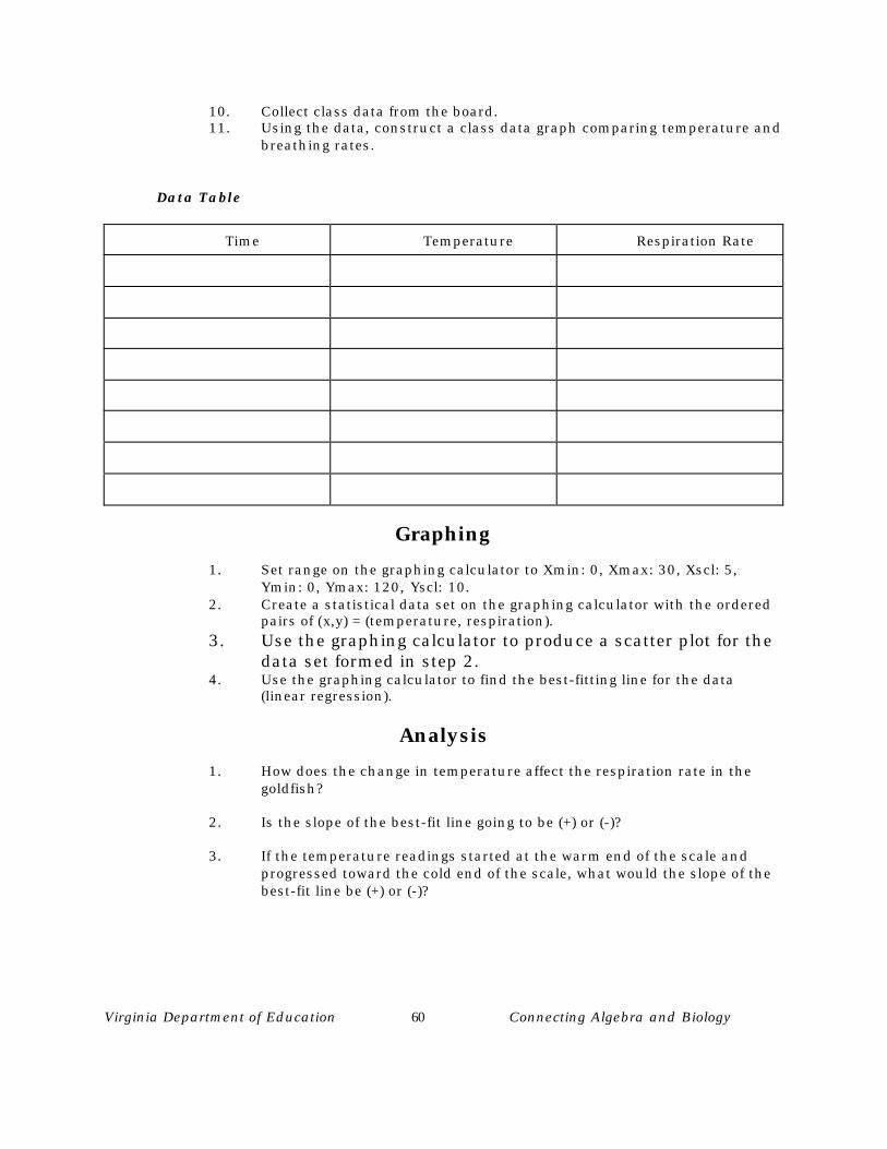
Virginia Department of Education 60 Connecting Algebra and Biology
10. Collect class data from the board.11. Using the data, construct a class data graph comparing temperature and
breathing rates.
Data Table
Time Temperature Respiration Rate
Graphing
1. Set range on the graphing calculator to Xmin: 0, Xmax: 30, Xscl: 5,Ymin: 0, Ymax: 120, Yscl: 10.
2. Create a statistical data set on the graphing calculator with the orderedpairs of (x,y) = (temperature, respiration).
3. Use the graphing calculator to produce a scatter plot for thedata set formed in step 2.
4. Use the graphing calculator to find the best-fitting line for the data(linear regression).
Analysis
1. How does the change in temperature affect the respiration rate in thegoldfish?
2. Is the slope of the best-fit line going to be (+) or (-)?
3. If the temperature readings started at the warm end of the scale andprogressed toward the cold end of the scale, what would the slope of thebest-fit line be (+) or (-)?

Virginia Department of Education 61 Connecting Algebra and Biology
4. Compare your individual graph with the class graph. Which graph is abetter indication of what is occurring? Explain why.
5. Name the two types of relationships that can exist in graphing variables.
6. What ultimately happens to goldfish in a pond as the water freezes?
CreditsRandolph Holland, Suffolk County Public SchoolsBill Lawrence, Danville City Public SchoolsWilburn Wilson, Suffolk County Public Schools
Virginia Department of Education 62 Connecting Algebra and Biology
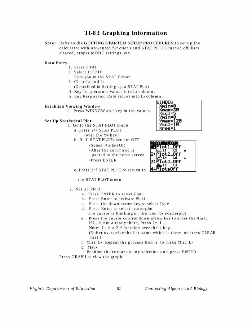
TI-83 Graphing Information
Note: Refer to the GETTING STARTED SETUP PROCEDURES to set up thecalculator with unwanted functions and STAT PLOTS turned off, listscleared, proper MODE settings, etc.
Data Entry 1. Press STAT
2. Select 1:EDITPuts you in the STAT Editor
3. Clear L1 and L2
(Described in Setting up a STAT Plot) 4. Key Temperature values into L1 column. 5. Key Respiration Rate values into L2 column.
Establish Viewing Window 1. Press WINDOW and key in the values.
Set Up Statistical Plot 1. Go to the STAT PLOT menu
a. Press 2nd STAT PLOT (over the Y= key)b. If all STAT PLOTs are not OFF
•Select 4:PlotsOff•After the command is
pasted to the home screen•Press ENTER
c. Press 2nd STAT PLOT to return to
the STAT PLOT menu
2. Set up Plot1 a. Press ENTER to select Plot1
b. Press Enter to activate Plot1c. Press the down arrow key to select Typed. Press Enter to select scatterplot
The cursor is blinking on the icon for scatterplot e. Press the cursor control down arrow key to enter the Xlist:
If L1 is not already there, Press 2nd L1.Note: L1 is a 2nd function over the 1 key.(Either overstrike the list name which is there, or press CLEAR first.)
f. Ylist: L2 Repeat the process from e. to make Ylist: L2
g. Mark Position the cursor on any selection and press ENTER
Press GRAPH to view the graph.
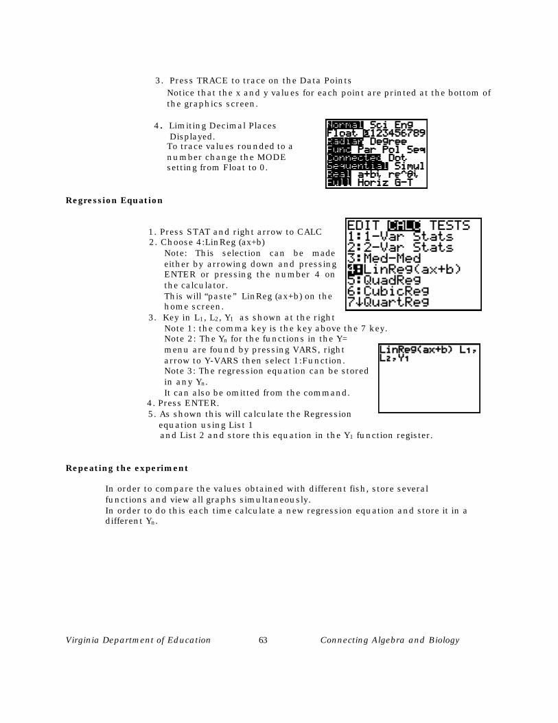
Virginia Department of Education 63 Connecting Algebra and Biology
3. Press TRACE to trace on the Data Points
Notice that the x and y values for each point are printed at the bottom of the graphics screen.
4. Limiting Decimal Places Displayed.To trace values rounded to anumber change the MODEsetting from Float to 0.
Regression Equation
1. Press STAT and right arrow to CALC 2. Choose 4:LinReg (ax+b)
Note: This selection can be madeeither by arrowing down and pressingENTER or pressing the number 4 onthe calculator.This will “paste” LinReg (ax+b) on thehome screen.
3. Key in L1, L2, Y1 as shown at the rightNote 1: the comma key is the key above the 7 key.Note 2: The Yn for the functions in the Y=menu are found by pressing VARS, rightarrow to Y-VARS then select 1:Function.Note 3: The regression equation can be storedin any Yn.
It can also be omitted from the command. 4. Press ENTER.
5. As shown this will calculate the Regression equation using List 1
and List 2 and store this equation in the Y1 function register.
Repeating the experiment
In order to compare the values obtained with different fish, store severalfunctions and view all graphs simultaneously.In order to do this each time calculate a new regression equation and store it in adifferent Yn.

Virginia Department of Education 64 Connecting Algebra and Biology
BRAIN STORM
Related SOL: BIO.1, BIO.2, BIO.3, BIO.9, A.7, A.15, A.17
Objective:The student will investigate and understand how populations evolve over time.
OverviewScientists have been able to study natural selection in peppered moths, Biston betularia, in England since the Industrial revolution. The peppered moth population was observed in the 1800's to be primarily made up of light-colored lichens covering the trees and rocks and found hiding places on the bark of the lichen-covered trees. With the rise of industry and the burning of fossil fuels, air pollution killed off the lichens and left the dark-colored bark exposed. What do you think happened in the population of light- and dark-colored moths over time? This laboratory will explore how to make predictions with the graphing calculator in order to test your hypothesis.
Materials
Graphing CalculatorDigital Camera...OptionalFlex Camera... Optional
Procedure
Use the table below to complete the list of activities.
TABLE #1:Year Number of light Number of dark
moths captured moths captured
2 537 1123 484 1984 392 2105 246 2816 225 3577 193 4128 147 5039 84 594
10 56 638

Virginia Department of Education 65 Connecting Algebra and Biology
ACTIVITIES:
1. Create a two variable statistical data set within the calculator with the ordered pair (x,y).
a) (x,y) = (year, number of light moths captured)b) (x,y) = (year, number of dark moths captured)
2. Use the graphing calculator to draw a scatter plot for each set of statistical data. Use the range Xmin = -1, Xmax = 12, Xscl = 1, Ymin = -1, Ymax = 640, Yscl = 1.
3. Use the graphing calculator to find the best fitting curve for the data. Try all regression equations available on the calculator, comparing the correlation coefficient (r) to determine which curve fits the data better.
y=_________________ r=__________________
4. Sketch the graph of the best fit curve of each.
5. Determine the slope of the line using the calculator. Then use the trace button to choose two points on the line. Use the slope formula to compute the slope manually. Compare the two answers.
6. Using the graph that represents the light moths captured, approximate in years and months when the light moths will become extinct. Explain your answer.
Credits:
Janece Bibby, Richmond City SchoolsMartha Cook, Richmond City SchoolsCatherine Robinson, Richmond City SchoolsDiane Williams, Richmond City Schools

Virginia Department of Education 66 Connecting Algebra and Biology
TI-83 Graphing Information
Note: Refer to the GETTING STARTED SETUP PROCEDURES to set up theCalculator with the unwanted functions and STAT PLOTS turned off,Lists cleared, proper MODE settings, etc.
Data Entry
1. Press STAT2. Select 1:EDIT
Goes into STAT Editor3. Clear L1, L2, L3
4. Enter Years into L1
5. Enter light moths into L2
6. Enter dark moths into L3
Set up STAT Plot1. Press 2nd STAT PLOT2. Press ENTER to select Plot13. Select scatter plot4. Enter L1 into Xlist5. Enter L2 into Ylist6. Press 2nd STAT PLOT7. Select Plot28. Enter L3 into Ylist
WINDOW Setting1. Press WINDOW2. Enter Xmin=0; Xmax=11; Xscl=1; Ymin=-50; Ymax=650; Yscl=50; Xres=1
Regression Equation1. Press STAT and right arrow to CALC2. Select #3 Med-Med.3. Key in L1, L2, Y1 to model the number of light moths.4. Press ENTER5. Press GRAPH to view the Eq superimposed on the STAT plot6. Repeat the process for List 1 and List 3 to get a model for the dark moths.7. Try other regression models to find a good fit.
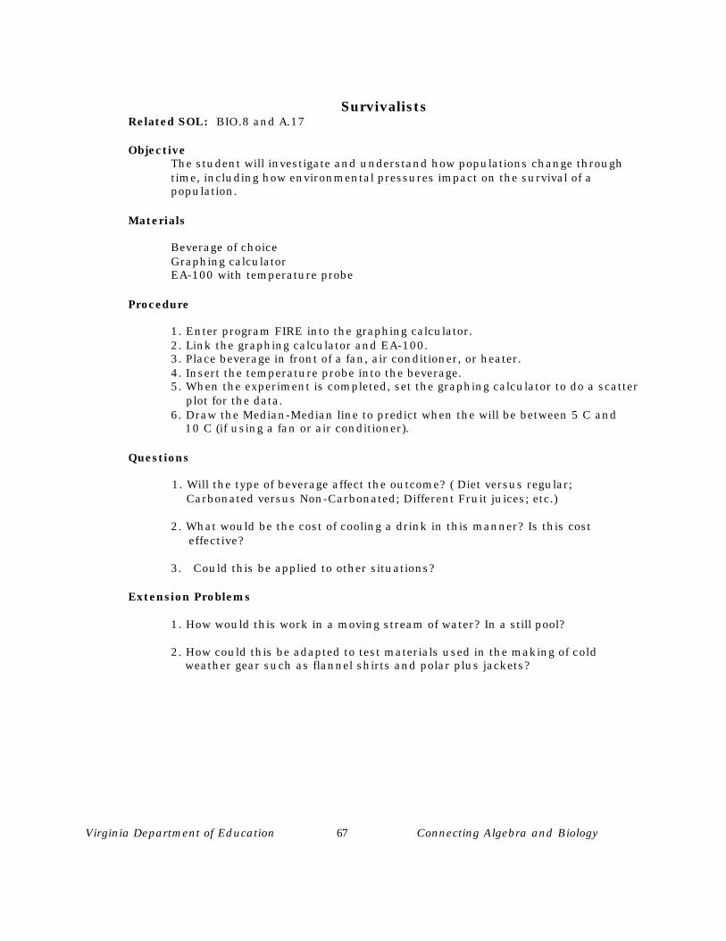
Virginia Department of Education 67 Connecting Algebra and Biology
SurvivalistsRelated SOL: BIO.8 and A.17
ObjectiveThe student will investigate and understand how populations change throughtime, including how environmental pressures impact on the survival of apopulation.
Materials
Beverage of choiceGraphing calculatorEA-100 with temperature probe
Procedure
1. Enter program FIRE into the graphing calculator.2. Link the graphing calculator and EA-100.3. Place beverage in front of a fan, air conditioner, or heater.4. Insert the temperature probe into the beverage.5. When the experiment is completed, set the graphing calculator to do a scatter plot for the data.6. Draw the Median-Median line to predict when the will be between 5 C and 10 C (if using a fan or air conditioner).
Questions
1. Will the type of beverage affect the outcome? ( Diet versus regular; Carbonated versus Non-Carbonated; Different Fruit juices; etc.)
2. What would be the cost of cooling a drink in this manner? Is this cost effective?
3. Could this be applied to other situations?
Extension Problems
1. How would this work in a moving stream of water? In a still pool?
2. How could this be adapted to test materials used in the making of cold weather gear such as flannel shirts and polar plus jackets?
Virginia Department of Education 68 Connecting Algebra and Biology
Problems and Solutions
1. Problem: The EA-100 would turn off prematurely Solution: Use the AC adaptor which will override the automatic turnoff.
2. Problem: The CFX-9850G Plus turns off prematurely. Solution: Press one of the directional keys every 20 - 30 minutes to keep it on.
3. Problem: The program starts but gives a command error.Solution: a) Check the program to make sure there are no errors in typing inlines of the program.
b) Check to make sure the set up of the equipment is right.
Credits
Nancy Bell, I.C. Norcom HSJ.Dianne Johnson, I.C. Norcom HSNancy Parker, John S. Battle HSWilliam Wynn III, Brunswick Sr. HS
Virginia Department of Education 69 Connecting Algebra and Biology
PROGRAM FIRE adapted for SURVIVALIST
{0}\->\List 6\Send(\List 6)\Cls{1,0}\->\List 6\Send(\List 6){1,1,7}\->\List 6\Send(\List 6)"PRESS TRIGGER ON DA""PUT PROBE IN CAN OF@ASODA UNTIL DONE@"PRESS EXE"{3,900,12,1}\->\List 6\Send(\List 6)\Disp\Receive(\List 1)\Receive(\List 2)\S-WindAuto\S-Gph1 \DrawOn,\Scatter,\List 1,\List 2,1,\Cross,\Blue\S-Gph2 \DrawOff\S-Gph3 \DrawOff\DrawStat0\->\Ymin0\->\Xmin30\->\Xscl5\->\Yscl\S-WindMan\DrawStat%End
%Header RecordFormat:TXTCommunication SW:0Data Type :PGCapacity:17File Name:RECEIVEGroup Name:Password:Option1:NLOption2:Option3:Option4:%Data Record\Receive(\List 1)\Receive(\List 2)
%End
Virginia Department of Education 70 Connecting Algebra and Biology
Hanging Around the Lake
ObjectiveThe student will investigate and understand how populations change with theirenvironment.
OverviewEven though we think of a lake as a single environment, it is actually made upof many smaller habitats. Each living thing in the lake has its own special needsfor survival- light, temperature, food, pH, oxygen levels, and water movement aresome examples. In this exercise, you will explore some of the physicalcharacteristics of a lake or pond and try to identify the type(s) of organisms thatlive in each of theses special habitats. You will learn how to identify and classifysome of the more common species found in the lake/pond.
Materials
Two small watercraftTwo graphing calculatorsA data collector interfaceA temperature probeA light probeA pH probeA ball of stringweights (100 g)Plastic bottlesPlankton netsSeine net (optional)White specimen traysMicroscope along with slides and cover slipsClassification books for reference
Procedure
1. Survey the lake and place the plastic bottles as float markers at points to be monitored.
Try to make measuring points at least fifty feet apart in all directions.2. Measure the water temperature, water pH and water clarity at each survey point.
Enter in data table.3. Measure depth of water at the survey point. Enter this information in the
data table.

Virginia Department of Education 71 Connecting Algebra and Biology
4. At each location identified,a. Collect some water with the plankton net to look at under the microscope.b. Use the identification books to try to identify any living organisms found.b. Use the seine net to trap larger organisms to identify. Set these in the
White specimen trays to study in the field or bring back to thelaboratory.
d. Remember to also collect and identify plant specimens.
5. As the lake is studied over several weeks, be sure to note any changes in the population(s) of any of the organisms.
Data Table
Survey Temp ofwater ©
PH inwater
Clarity ofwater
Depth ofwater (m)
No. of fish No. ofdifferentkinds ofspecies
Analysis
Use the graphing calculator:
1. Set the program of the graphing calculator on Receive to load data. In the program Receive, set-up List 1 - List 6.
2. Create a statistical data set on the graphing calculator using all six fileswhen reading data from the lake.

Virginia Department of Education 72 Connecting Algebra and Biology
3. Use the graphing calculator to produce a scatter plot for the data set for each
file.
4. If the class needs to see the graph from each reading, store each picture,Then recall each on File 6 to show the change in the data.
5. Use the graphing calculator to find the best-fit line for the points (med-med).
Questions
1. How would extreme temperature changes effect the aquatic population?
2. How will the slope of the temperature graph change as the temperature increases?
3. What effect would you expect with increasing water pH?
4. What is the relationship of the temperature and the pH?
.Credits
Alvin Coleman, Chesapeake City Public SchoolsMary Copeland, Chesapeake City Public SchoolsDonald Rima, Hampton City Public SchoolsEleanor Teed, Greene County Public Schools

Virginia Department of Education 73 Connecting Algebra and Biology
Let There Be LightObjectiveThe student will be able to define and recognize the slope of a lineThe student will be able to analyze data to form a conclusion about the effects oferosion.
OverviewWhen development occurs near waterways and ponds careful considerationshould be taken to prevent excess soil from entering the water. Sediment mixeswith the water, making the water turbid (cloudy/muddy).This turbidity reducesthe amount of sunlight entering the water by acting as a filter. The smallsubmerged aquatic vegetation (SAV) cannot obtain enough light for sufficientphotosynthesis activity. The result is the death of the SAVs. As they die anddecay, carbonic acid is produced. If many plants die, it may cause the water tobecome more acidic (lowering the pH). Another problem that may result from thedeath of SAVs is the increase of nitrogen compounds in the water. This acts as afertilizer and causes algal blooms. The decaying SAVs cause a reduction in theamount of dissolved oxygen (the amount of oxygen in the water available toanimals such as fish and zooplankton). Hence, a simple thing such as erosionmay have a major impact on the environment. In this activity, you will simulatethe effect of turbidity.
Materials
1 link cord Waterone plastic tub Soilflashlight 1 EA-100 and 1 light probemeasuring cup Spoon or stirring rod5 containers for water and soil Tapeblock or piece of styrofoam to stabilize the light probestopwatch or watch with a second hand 1 CFX-9850+ calculator
Procedure1. On a level surface, place the plastic tub.2. Plug light probe into Channel 1 of the EA-100.3. Position and secure the flashlight on the level surface of one side of the plastictub.4. Position and secure the light probe on the other side of the plastic tub. The l light probe should be the same level as the most intense beam of the flashlight. (Use the block of wood to raise the light probe to appropriate level if needed.)5. Fill 4 containers with 1/4 cup of dirt.
Virginia Department of Education 74 Connecting Algebra and Biology
6. Fill the 5th container with 3 quarts of water.7. Push the red ON button to activate the EA-100.8. Press SHIFT MODE to enter the setup.9. The first setting is the number of seconds wanted between samples. Use the dataLOG key to scroll forward through the choices until you reach 20 seconds . Press TRIGGER to make your choice.
10. The next setting is the total number of samples that desired. Use the dataLOG key to scroll through the choices until you reach 20. Press TRIGGER to make your choice.11. The final setting on the EA-100 is the time recording mode. Use the dataLOG key to choose A1" so the actual times will be recorded. PressTRIGGER to make your choice.12. NOTE: This lab is designed to take 3 samples every minute forapproximately 7 minutes. For the first minute your tub should be empty.After the first minute add water to the tub. During the next 4 minutes add one container of dirt each minute. DO NOT add dirt directly in front of the flash light because this could give a false reading.13. We are now ready to start the experiment.14. Turn on the flashlight.15. Press the TRIGGER to start sampling. The word Asampling@ should be flashing on the screen at this time. ADone@ will appear on the screen of the EA-100 when the sampling is complete.16. Connect the CFX-9850+ to the EA-100 with the link cord. Be sure the cables are pushed in securely. Turn the calculator ON.17. Select PRGM from the main menu and push EXE.18. Use the arrow key to locate your Receive program. F1(EXE). The little box in the right hand corner means that the calculator is thinking.19. When the screen says DONE, you are ready to view your graph. Choose STAT from the main menu and push EXE. F1(Grph); F6(SET); highlight Graph Type; F2(xy); scroll down to Mark Type; select F3( ); EXIT; SHIFT MENU(setup);highlight Stat Wind; F1(Auto);EXIT;F1(Grph). The graph should appear on the screen. Sketch the graph from the view window.
Analysis/Questions
1. Explain what happened in the data in the following portions of the lab and why
a. when the water was added? b. when the first 1/4 cup of soil was added?
c. When the last 1/4 cup of soil was added?
2. Sketch the graph in the space below. Now highlight the following with the appropriate color:
a. Use blue to show the location of a slope of 0.b. Use red to show the location of a negative slope.c. Use green to show the location of the positive slope.
Virginia Department of Education 75 Connecting Algebra and Biology
Compare your actual graph to that of your prediction in the Getting Readysection.
3. How many changes occurred in the graph and explain what happened to cause the change?
4. Based on the data from the graph, will the graph ever reach zero? Whatwould
be the difference between a graph of a pond and that of a river?
Extensions
1. If the graph were to start at the point of erosion, what type of function does the data resemble?
2. Based on your understanding of the effects of erosion on the clarity of water in rivers and streams, what do you anticipate will happen to the nekton and zooplankton in those areas? Write an informational letter to your local representative describing the ramifications of residential and commercial development on waterways.
Getting Ready
1. What are the two variables in this experiment? What is the independent variable? The dependent variable?
2. What type of graph do you anticipate with the following trials:*an empty tub?*a tub with water?*a tub with water and 1/4 cup of soil?*a tub with water and 1 cup of soil?
Sketch each graph below in a different color and label.
CreditsRobin Carey, west Point Public SchoolsAnne Fary, Gloucester County Public SchoolsTeresa Haskiell, Gloucester County Public SchoolsHelen Luster, Portsmouth City Public Schools

Virginia Department of Education 76 Connecting Algebra and Biology
TI-83 InformationCBL program
The following program for the CBL can be keyed into the TI-83 and then run. It will giveinstructions to the CBL and then get the data from the CBL. It is very basic, so thestudent will need to know what the lab is about, and that the CBL is simply gatheringthe light intensity and time data. The calculator will get the actual time data into listL1 and the corresponding light intensity data into list L2. As soon as the experiment iscomplete the calculator will display a scatterplot of the data (time, light intensity)
In order to enter a program•Press PRGM key•Right arrow to NEW
•Key in a name such as SOIL•Press ENTER•Key in the Program•Other students can
link.
:PlotsOff:FnOff:ClrHome:Send ({1,0}):Send ({1,1,12,0}):Disp “HIT [ENTER]”:Pause:Send({3,20,22,0,0,0,0,1,0}):Get (L2):Get (L1):Plot1(Scatter,L1,L2,+):ZoomStat
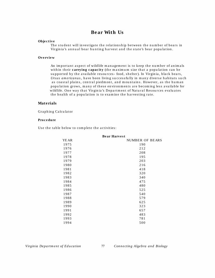
Virginia Department of Education 77 Connecting Algebra and Biology
Bear With Us
ObjectiveThe student will investigate the relationship between the number of bears inVirginia’s annual bear hunting harvest and the state’s bear population.
Overview
An important aspect of wildlife management is to keep the number of animalswithin their carrying capacity (the maximum size that a population can besupported by the available resources- food, shelter). In Virginia, black bears,Ursus americanus, have been living successfully in many diverse habitats such as coastal plains, central piedmont, and mountains. However, as the humanpopulation grows, many of these environments are becoming less available for
wildlife. One way that Virginia’s Department of Natural Resources evaluatesthe health of a population is to examine the harvesting rate.
Materials
Graphing Calculator
Procedure
Use the table below to complete the activities:
Bear Harvest YEAR NUMBER OF BEARS
1975 1901976 2121977 2081978 1951979 2031980 2161981 4181982 3201983 3401984 4751985 4801986 5251987 5401988 5791989 6251990 3231991 6571992 4831993 7811994 500

Virginia Department of Education 78 Connecting Algebra and Biology
Enter the data into the Graphing Calculator using the following steps:1. Go to STAT on the MENU screen2. Enter the years into List 1.3. Enter the number of bears into List 2.4. Make sure your pairs of years and bear harvest match.
Graphing
To make a Scatter Plot:1. Remain in STAT.2. Press F1 (Graph), F6 (SET)3. Enter choices: Graph 1 (F1)
Arrow down to Graph Type, press F1At x-List, press F1At y-List, press F2Arrow down to Frequency, press F1 and press EXEPress F1 (Graph1) and the scatter plot appears.
4. Press F2 for linear interpretation and F6 for best fit graph.5. Transfer the linear equation to the GRAPH menu for interpretation and predictions.
To make a Histogram from the data:1. Make sure you are in STAT.2. Press F1 (Graph), F6 (Set) and change Graph Type to Histogram (F6), press F13. At x-List, press F1.4. At Frequency, press F3 (List 2), press EXE, EXIT, then F6.5. Press F4 (SEL), make sure Graph 1 is ON (F1), press Draw (F6)6. Screen set interval appears. Change Pitch to 1, press EXE , press Draw (F6).
BEARO!----Your Histogram
Analysis/Questions
1. Based on the data what appears to be happening to the bear population inthe last 20 years?
2. As a result of the harvests predict what the harvest could be in the next 5 to 10 years.
3. What are some possible habitat changes that would affect the bearpopulation in VA?
4. What is the most likely region in VA where bears may still successfully reside in 10 years?
4. What wildlife management methods and policies could Virginia institute thatwould increase and/or stabilize Virginia’s bear population?
5. Considering the bear carrying capacity in Virginia, state one possiblereason why the bear harvest decreased from 1989 to 1990.
Virginia Department of Education 79 Connecting Algebra and Biology
Additional Bear Facts
1. Native Americans and the early Virginia settlers used bears for many valuablecommodities. Bear skins were made into heavy winter robes, moccasins, andblankets. Twisted bear gut was made into bowstrings. Teeth and claws wereused as ornaments. Bear fat was used as butter, body and hair oil, and in themaking of body paints.
2. The normal range an animal will frequent is called a home range. Home rangemust provide food, water, den sites, and adequate concealment for the bearpopulation. An adult male’s home range is approximately 15 sq. miles, anadult female’s is approximately 10 sq. miles.
3. Bears are omnivorous, and opportunistic feeders. They will readily feed on thefood that is available to them. In the spring, they will consume grasses, forbs,and other plants until soft mast, such as berries, pin cherries, etc. arepresent. Fall foods are generally hard mast, consisting of acorns, hickorynuts, and beechnuts.
Credits
Mildred Calhoun, B.T. Washington H.S., NorfolkSusan Currier, Petersburg H.S., PetersburgJacqueline Gooden-Seay, Petersburg H.S., PetersburgLarry Turner, Spotswood H.S. Rockingham County
Virginia Department of Education 80 Connecting Algebra and Biology
TI-83 Graphing Information
Note: Refer to the GETTING STARTED SETUP PROCEDURES to set up theCalculator with the unwanted functions and STAT PLOTS turned off,Lists cleared, proper MODE settings, etc.
Data Entry
7. Press STAT8. Select 1:EDIT
Goes into STAT Editor9. Clear L1, L2, L3
10. Enter Years into L1
11. Arrow over and up onto the L2 heading12. Key in L1-1975. Press ENTER to fill in the column13. Enter Bear Harvest values into L3
Set up STAT Plot9. Press 2nd STAT PLOT10. Press ENTER to select Plot111. Select scatter plot12. Enter L2 into Xlist13. Enter L3 into Ylist
WINDOW Setting3. Press WINDOW4. Enter Xmin=0; Xmax=20; Xscl=1; Ymin=0; Ymax=800; Yscl=100; Xres=15. Press GRAPH to view the graph
Regression Equation8. Press STAT and right arrow to CALC9. Select #3 Med-Med.10. Key in L2, L3, Y1
11. Press ENTER12. Press GRAPH to view the Eq superimposed on the STAT plot
Set up a Histogram1. Go to STAT Plot1 and turn it off2. Set up STAT Plot2 :
• Choose histogram as the TYPE (icon 3)• Xlist: L2
• Freq: L3
3. Press GRAPH4. Press TRACE. This will tell the number of bears in each year.
Virginia Department of Education 81 Connecting Algebra and Biology
An Interdisciplinary Deer and Human Population Study
ObjectiveThe student will investigate what environmental problems arise due to overpopulation and competition for resources.
OverviewEcology is the study of how organisms interact with their environment- both thebiotic (living) and the abiotic (non-living such as temperature and light).Climate, which is made up of temperature, light, wind, and water, affects wherea population may settle. Virginia falls mostly within the temperate forest climate.Deer do well in this type of environment, but so do many other animals. Thismay lead to competition between the deer themselves or competition between adifferent species for food, shelter, and other resources. A basic rule in ecology iscalled the competitive exclusion principle which is defined in Campbell’sFourth Edition Biology as: when the populations of two or more species competefor the same limited resources, one population will use the resources moreefficiently and have a reproductive advantage that will eventually lead to theelimination of the other population.In this laboratory, you will explore what happens to a deer population whenresource such as food becomes scarce. Is this due to a loss of habitat? To achange in climate? Or are we that other species?
Materials
Graphing CalculatorsCheckerboard Grid
Procedure
The following programs will be needed:Random Numbers:Menu (1), optn, F6, F4, F2, EXIT, (enter #), F3, F4 + 1, EXE
Note: To begin game use 2 and the first 32 numbers.
Graphing
Histogram:Menu (2), Highlight the List you want to use, F1 (graph), F6 (Set), F6, F1([Graph Type]-hist) F1([xList]-List1), EXIT, F1 (Set interval-chooseappropriate #s), F6 (Draw), F1 (view statistics)

Virginia Department of Education 82 Connecting Algebra and Biology
Teacher Notes:
This entire lesson plan may be down loaded at: http://www.gene.com.The original activity has been modified to make use of the graphing calculatortechnology. Tokens will be used instead of checkers. We recommend the use ofscripts to present the six events. The use of the random number generator onthe calculator will replace the random drawing of tokens and also will be used todetermine the sex of fawns. Instead of a hunting screen (as described in theoriginal plan) we will again use the random number generator to determinewhich of the 64 possible territories will be hunted. The number of huntersshould be determined by each group.
Migration is when a deer on the perimeter of the park occupying a light coloredsquare moves to an adjacent dark square or leaves the park. At that time anydeer occupying light squares should be considered to have starved to death andthe pieces should be removed. New deer occupy any dark perimeter squares.Then the final count for population is done and the data entered for themigration.
Credits
Rodney Berry, Richmond City Public SchoolsJames Gardner, Mecklenburg County Public SchoolsGlenn Gould, Liberty H.S., Fauquier CountyRobert A. Spain, Hampton City Public SchoolsJoseph D. Sweat, Hampton City Public Schools
Virginia Department of Education 83 Connecting Algebra and Biology
Examination of the Hardy-Weinberg Theorem
ObjectivesAt the completion of this laboratory, students should be able to:
1. Calculate allele and genotype frequencies using the Hardy-Weinberg theorem.
2. Discuss the effect of natural selection on allelic frequencies.
3. Discuss the relationship between evolution and changes in allele frequencies, as measured by the Hardy-Weinberg Law of Genetic Equilibrium.
Overview
In 1908 the Englishman G.H. Hardy and the German W. Weinbergindependently suggested that evolution could be viewed as changes in thefrequency of alleles (one member of a pair of genes) in a population of organisms.The Hardy-Weinberg Law of Genetic Equilibrium for a population states that thefrequency of the alleles or the genotypes in the gene pool (the total alleles in thepopulation at that time) remain constant unless factors other than the sheerrandomness of meiosis or fertilization occur.A population that is in equilibrium must meet these five criteria:
1. The population is very large.2. Mating is random.3. No mutation occurs.4. The population remains isolated-no migration or emigration.5. No natural selection occurs.
Materials
Graphing Calculator2 3"X5" index cards labeled a2 3"X5" index cards labeled Aextra cards labeled Aextra cards labeled ahandoutWriting utensil
Procedure
1. Record the number of people in the class who are tongue rollers and who arenot tongue rollers.
# of tongue rollers
Virginia Department of Education 84 Connecting Algebra and Biology
# of non-tongue rollers
2. Each member of the class will receive four cards. Two cards will have the letter A printed on them and the other two the letter a. A represents the dominant allele and a is a recessive allele. Each student will work with a partner. Each mate contributes one allele towards the next generations trait.
3. Turn the cards over, shuffle, and take the card on top to contribute to the production of the first offspring. Your partner should do the same. Put the two cards together. You are now the proud parents of the first offspring. One of you should record the genotype of this offspring in the Generation 1 row of the table. Each student pair must produce two offspring, so all four cards must be reshuffled and the process repeated to produce a second offspring.
4. Your partner should then record the genotype of the second offspring in his/her table. The very short reproductive career of this generation is over. You and your partner now become the next generation of the two offspring. That is, student 1 assumes the genotype of the first offspring and student 2 assumes the genotype of the second offspring.
5. Each student should obtain, if necessary, new cards representing the alleles in his/her respective gametes after the process of mating. Each participant should randomly seek out another person with whom to mate in order to produce the offspring for he next generation. The sex of your partner does not matter, nor does the genotype. You should follow the same mating procedures as for the first generation, being sure to record your new genotype after each generation in the table. Class data should be collected after each generation for five generations. At the end of each generation, remember to record the genotype that you have assumed. Class data will be collected and recorded after each generation by asking you to raise your hand to report your genotype.
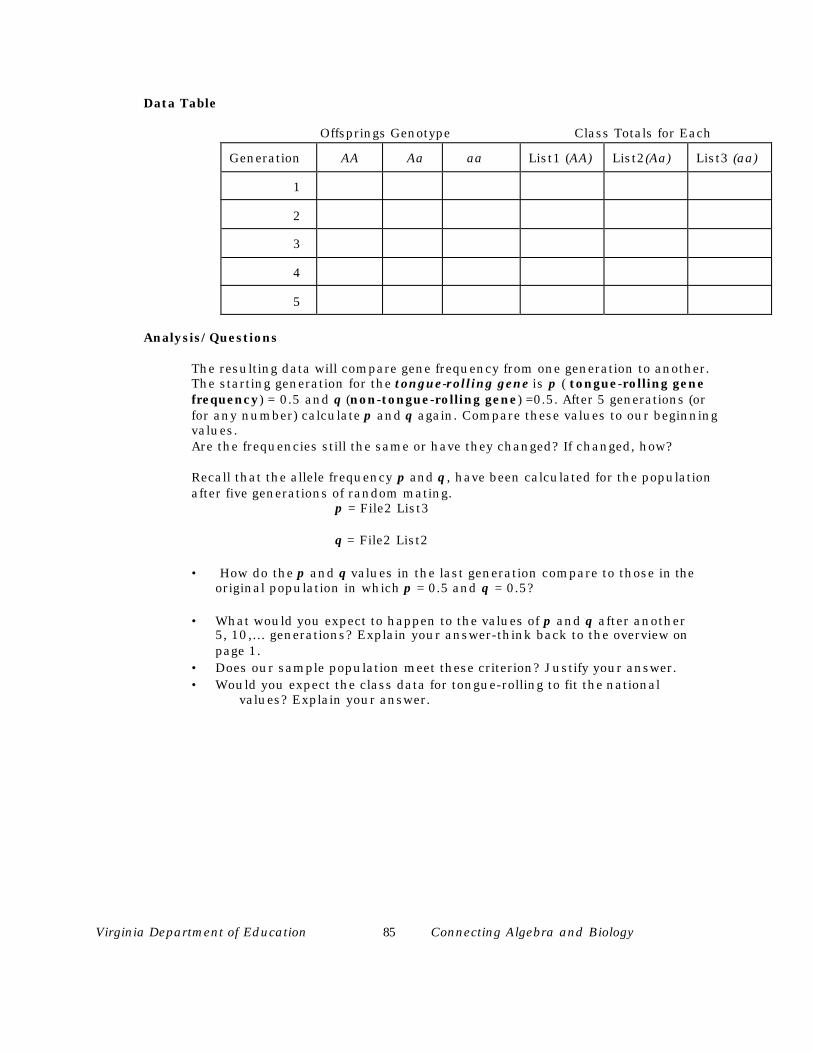
Virginia Department of Education 85 Connecting Algebra and Biology
Data Table
Offsprings Genotype Class Totals for Each
Generation AA Aa aa List1 (AA) List2(Aa) List3 (aa)
1
2
3
4
5
Analysis/Questions
The resulting data will compare gene frequency from one generation to another.The starting generation for the tongue-rolling gene is p ( tongue-rolling genefrequency) = 0.5 and q (non-tongue-rolling gene) =0.5. After 5 generations (orfor any number) calculate p and q again. Compare these values to our beginningvalues.Are the frequencies still the same or have they changed? If changed, how?
Recall that the allele frequency p and q, have been calculated for the populationafter five generations of random mating.
p = File2 List3
q = File2 List2
• How do the p and q values in the last generation compare to those in theoriginal population in which p = 0.5 and q = 0.5?
• What would you expect to happen to the values of p and q after another 5, 10,... generations? Explain your answer-think back to the overview on
page 1.• Does our sample population meet these criterion? Justify your answer.• Would you expect the class data for tongue-rolling to fit the national
values? Explain your answer.
Virginia Department of Education 86 Connecting Algebra and Biology
KEYSTROKES FOR ENTERING THE LISTS FOR HARDY-WEINBERG LAB
Use the LIST menu (4).
In File 1For List1: enter the data from your table List1 (AA); press EXE after eachentry.
For List2: enter the data from your table List2 (Aa); press EXE.
For List 3: enter the data from your table List3 (aa); press EXE.
For List 4 (frequency of AA):Arrow to the top of List 4 so that List 4 is highlighted. To insert the
equation, press OPTN F1, then F1 again to write List so that on yourscreen you enter List1/(List1 + List2 +List3). EXE.
For List 5 (frequency of Aa): Arrow to the top of List 5 so that List 5 is highlighted. To insert the
equation use F1 to write List so that on your screen you enter List2/(List1 + List2 + List3). EXE
For List 6 (frequency of aa): Arrow to the top of List 6 so that List 6 is highlighted. To insert the equation use F1 to write List so that on your screen you enter
List 3/(List1 + List2 + List3). EXE
Now we need to go to File 2 to create the rest of the needed Lists because wehave used all the lists in File 1. Since we cannot reference a list from File 1 touse in creating lists in another file, write List 6 from File 1 on a piece of paper.Change your calculator to File 2 by pressing SHIFT Menu F2 EXE.
In File 2
For List 1 (frequency of aa):Enter the handwritten data (File 1 List 6)
For List 2 ( a or q): Arrow to the top of List 2 so that List 2 is highlighted.
To insert the equation press SHIFT x^2 for the .Then OPTN F1 then F1 again to write List then 1 EXE.
For List 3 (p): Arrow to the top of list 3 so that List 3 is highlighted. To insert the equation, press 1 - F1 2 EXE.
For List 4 (p^2): Arrow to the top of List 4 so that List 4 is highlighted. To insert the equation, press F1 then 3 then x^2. EXE

Virginia Department of Education 87 Connecting Algebra and Biology
For List 5 ( 2pq):Arrow to the top of List 5 so that List 5 is highlighted. Insert theequation 2List3List2 EXE
For List 6 ( p^2 + 2pq + q^2):Arrow to the top of List 6 so that List 6 is highlighted. Insert theequation List4 + List5 + List1 EXE
Credits
Larry Arbogast, Orange County Public SchoolsDwight D. Pascal, Orange County Public SchoolsAmy Stone, Virginia Beach City Public SchoolsLynne Uebelhoer, Virginia Beach City Public Schools
Virginia Department of Education 88 Connecting Algebra and Biology
TI-83 Information
Note: Refer to the GETTING STARTED SETUP PROCEDURES to set up your calculator with unwanted functions and STAT PLOTS turned off, lists cleared, proper MODE settings, etc.
STAT Editor set up:
1. Press STAT2. Select 1:EDIT3. Clear L1 through L6
4. Arrow over to L6 and up onto the heading5. Press the right arrow one more time to open a new list position6. Press ENTER
The cursor will be blinking in the Name position at the bottom of the screen.
7. Press the ) key to record the L8. Press the ALPHA key to exit ALPHA mode9. Press the number 7. L7 is now set.10. Repeat the process in steps #5- #9 for setting up L8 through L10
Data Entry List 1: Enter the data from table List 1 (AA)
List 2: Enter the data from table List 2 (Aa) List 3: Enter the data from table List 3 (aa) List 4: Frequency of AA
• Arrow to the heading for List 4• Key in L1/(L1 + L2 + L3)• Press ENTER
List 5: Frequency of Aa• Arrow to the heading for List 5• Key in L2/(L1 + L2 + L3)• Press ENTER
List 6: Frequency of aa• Arrow to the heading for List 6• Key in L3/(L1 + L2 + L3)• Press ENTER
List 7: for p2
• Arrow to the top of L7
• Press 2nd 1 for L1
• Press the x2 key• Press ENTER
List 8: for 2pq
• Arrow to the top of L8
• Press 2* L1 L3
• Press ENTER

Virginia Department of Education 89 Connecting Algebra and Biology
List 9: for q2
• Arrow to the top of L9
• Press L3
• Press the x2 key• Press ENTER
List 10: for p2 + 2pq + q2
• Arrow to the top of L10
• Press L7 + L8 + L9
• Press ENTER

Virginia Department of Education 90 Connecting Algebra and Biology
Texas Instruments TI-83Data Analysis
I. Getting Started Setup Procedures
A. Calculator Display Contrast
1. Darken Display• Press and release the yellow 2nd key in the upper left corner of the
calculator.
• Press and hold down the “cursor move” up arrow key on the upper right side of the calculator key pad. The display should darken. 2. Lighten Display
• Press and release the yellow 2nd key.• Press and hold down the “cursor move” down arrow key.
3. Numerical Indicator•• A number between 0 and 9 will appear in the upper
right corner of the calculator screen.• The number will be increasing as the display
darkens/decreasing as the display lightens. 4. Repeat as necessary
•• This process can be repeated until the contrast is to your liking.• If the number is 8 or 9 you should change batteries soon.
B. Menu Selections
1. Pressing the number or pressing ENTER•• When making a selection from a menu you can either Press the # of the desired selection
or Down arrow to highlight the selection # and then press ENTER
Example: Print a random integer between 1 and 10. Press the MATH key Right arrow to PRB Down arrow or press 5
NOTE: Often this process will “paste” the command on the home screen of the calculator. The command is not executed until you press ENTER. If you press CLEAR it will be removed
from the screen without being executed.
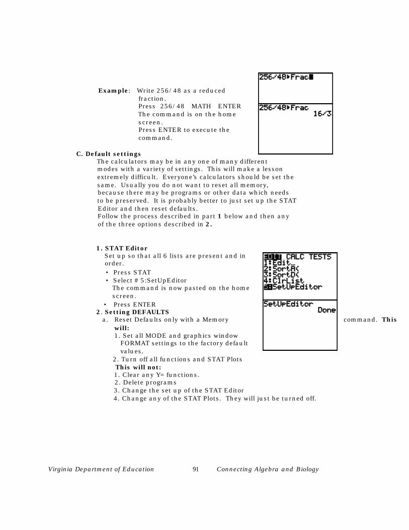
Virginia Department of Education 91 Connecting Algebra and Biology
Example: Write 256/48 as a reduced fraction. Press 256/48 MATH ENTER
The command is on the home screen. Press ENTER to execute the command.
C. Default settings The calculators may be in any one of many different modes with a variety of settings. This will make a lesson extremely difficult. Everyone’s calculators should be set the same. Usually you do not want to reset all memory, because there may be programs or other data which needs to be preserved. It is probably better to just set up the STAT Editor and then reset defaults. Follow the process described in part 1 below and then any of the three options described in 2.
1. STAT Editor Set up so that all 6 lists are present and in order.
• Press STAT • Select # 5:SetUpEditor The command is now pasted on the home screen. • Press ENTER
2. Setting DEFAULTSa. Reset Defaults only with a Memory command. This
will:1. Set all MODE and graphics window
FORMAT settings to the factory default values.
2. Turn off all functions and STAT Plots This will not:
1. Clear any Y= functions. 2. Delete programs 3. Change the set up of the STAT Editor 4. Change any of the STAT Plots. They will just be turned off.

Virginia Department of Education 92 Connecting Algebra and Biology
Reset Defaults:
• Press 2nd MEM (the + key)• Select #5: Reset• Select #2: Defaults• Select #2: Reset
b. Verify/Change all MODE and FORMAT settings individually.
• Press MODEArrow down and pressENTER on each line sothat all selections on theleft are highlighted.
• Press 2nd FORMAT(over the ZOOM key in thetop row)Arrow down and pressENTER on each line sothat all selections on theleft are highlighted.

Virginia Department of Education 93 Connecting Algebra and Biology
c. Run a Defaults program. One version is listed below
PROGRAM:DEFAULTS:Normal:Float:Radian:Func:Connected:Sequential:Real:Full:RectGC:CoordOn:GridOff:AxesOn:LabelOff:ExprOn:FnOff:PlotsOff:ClrDraw:ClrHome
II. Setting Up A STAT PLOT
A. Preliminaries
1. Set up STAT Editor and set Defaults as described in the previous section 2. Turn off or clear out
unwanted functions.• Press Y= key• To clear out functions:
Press CLEAR Down arrow and repeat
3. Deactivate functions• Position cursor over the =

Virginia Department of Education 94 Connecting Algebra and Biology
• Press ENTERIf the = ishighlighted,the function isactive.If the = is nothighlighted,
the function is turned off or deactivated.
4. Turn off all STAT PLOTS.
• Press 2nd STAT PLOT• Select 4:PlotsOff
This pastes command to the home screen.
• Press ENTER to execute the command
B. Establish a WINDOW
1. Review your experiment.2. Determine which is the independent
variable. This will be the Xlist
3. Determine which is the dependent variable. This will be the Ylist
4. Review the data values5. Set up the range of values for the horizontal
(X) and vertical (Y) axes.
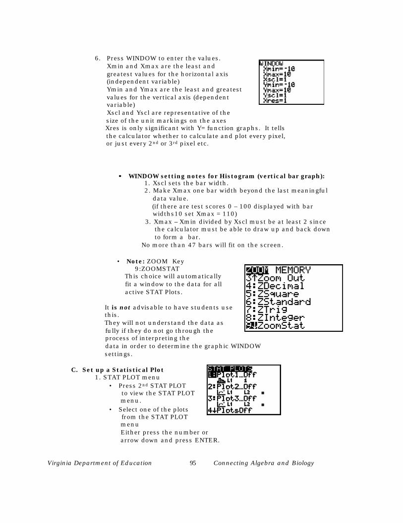
Virginia Department of Education 95 Connecting Algebra and Biology
6. Press WINDOW to enter the values.Xmin and Xmax are the least andgreatest values for the horizontal axis(independent variable)Ymin and Ymax are the least and greatestvalues for the vertical axis (dependentvariable)Xscl and Yscl are representative of the
size of the unit markings on the axes Xres is only significant with Y= function graphs. It tells
the calculator whether to calculate and plot every pixel, or just every 2nd or 3rd pixel etc.
•• WINDOW setting notes for Histogram (vertical bar graph): 1. Xscl sets the bar width.
2. Make Xmax one bar width beyond the last meaningful data value.
(if there are test scores 0 – 100 displayed with bar widths10 set Xmax = 110)
3. Xmax – Xmin divided by Xscl must be at least 2 since the calculator must be able to draw up and back down to form a bar.
No more than 47 bars will fit on the screen.
• Note: ZOOM Key 9:ZOOMSTAT
This choice will automatically fit a window to the data for all active STAT Plots.
It is not advisable to have students use this. They will not understand the data as
fully if they do not go through the process of interpreting the
data in order to determine the graphic WINDOW settings.
C. Set up a Statistical Plot 1. STAT PLOT menu
• Press 2nd STAT PLOT to view the STAT PLOT
menu.
• Select one of the plots from the STAT PLOT
menu Either press the number or arrow down and press ENTER.
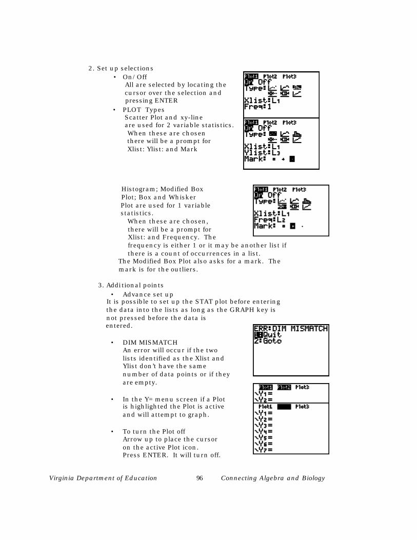
Virginia Department of Education 96 Connecting Algebra and Biology
2. Set up selections• On/Off
All are selected by locating the cursor over the selection and pressing ENTER
• PLOT Types Scatter Plot and xy-line
are used for 2 variable statistics. When these are chosen there will be a prompt for Xlist: Ylist: and Mark
Histogram; Modified Box Plot; Box and Whisker Plot are used for 1 variable statistics.
When these are chosen, there will be a prompt for Xlist: and Frequency. The frequency is either 1 or it may be another list if there is a count of occurrences in a list.
The Modified Box Plot also asks for a mark. The mark is for the outliers.
3. Addi tional points
• Advance set up It is possible to set up the STAT plot before entering the data into the lists as long as the GRAPH key is not pressed before the data is entered.
• DIM MISMATCH An error will occur if the two lists identified as the Xlist and Ylist don’t have the same number of data points or if they are empty.
• In the Y= menu screen if a Plotis highlighted the Plot is activeand will attempt to graph.
• To turn the Plot off Arrow up to place the cursor on the active Plot icon.
Press ENTER. It will turn off.
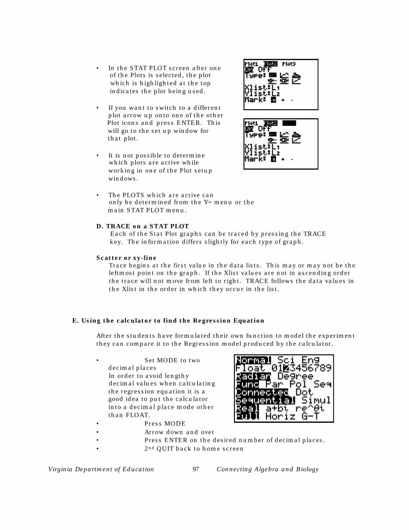
Virginia Department of Education 97 Connecting Algebra and Biology
• In the STAT PLOT screen after one of the Plots is selected, the plot
which is highlighted at the top indicates the plot being used.
• If you want to switch to a different plot arrow up onto one of the other Plot icons and press ENTER. This will go to the set up window for that plot.
• It is not possible to determine which plots are active while
working in one of the Plot setup windows.
• The PLOTS which are active can only be determined from the Y= menu or the
main STAT PLOT menu.
D. TRACE on a STAT PLOT Each of the Stat Plot graphs can be traced by pressing the TRACE key. The information differs slightly for each type of graph.
Scatter or xy-lineTrace begins at the first value in the data lists. This may or may not be theleftmost point on the graph. If the Xlist values are not in ascending orderthe trace will not move from left to right. TRACE follows the data values inthe Xlist in the order in which they occur in the list.
E. Using the calculator to find the Regression Equation
After the students have formulated their own function to model the experimentthey can compare it to the Regression model produced by the calculator.
• Set MODE to twodecimal places
In order to avoid lengthy decimal values when calculating the regression equation it is a good idea to put the calculator into a decimal place mode other
than FLOAT.• Press MODE• Arrow down and over• Press ENTER on the desired number of decimal places.• 2nd QUIT back to home screen
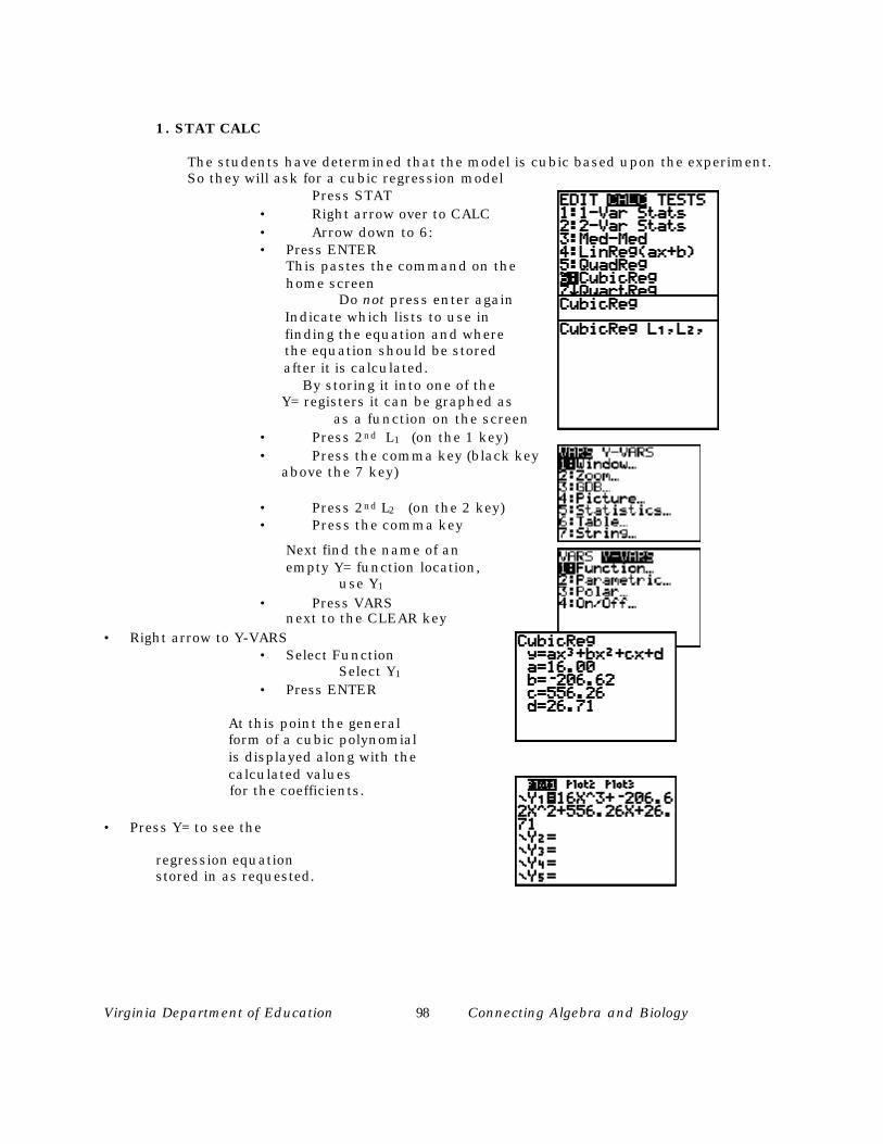
Virginia Department of Education 98 Connecting Algebra and Biology
1. STAT CALC
The students have determined that the model is cubic based upon the experiment.So they will ask for a cubic regression model
Press STAT• Right arrow over to CALC• Arrow down to 6:• Press ENTER
This pastes the command on thehome screen
Do not press enter again Indicate which lists to use in
finding the equation and where the equation should be stored after it is calculated.
By storing it into one of the Y= registers it can be graphed as
as a function on the screen• Press 2nd L1 (on the 1 key)• Press the comma key (black key above the 7 key)
• Press 2nd L2 (on the 2 key)• Press the comma key
Next find the name of anempty Y= function location,
use Y1
• Press VARSnext to the CLEAR key
• Right arrow to Y-VARS• Select Function
Select Y1
• Press ENTER
At this point the generalform of a cubic polynomialis displayed along with thecalculated values
for the coefficients.
• Press Y= to see the
regression equationstored in as requested.

Virginia Department of Education 99 Connecting Algebra and Biology
View the graphs of the STAT PLOT and the Regression Equation superimposed.
• Press GRAPH • Press TRACE The TRACE cursor will always go to the first
active STAT PLOT first.
• Press down arrow to TRACE on the function.
The following histogram and box and whisker plots are created with thesmall sample data set shown in List 4. Two screens are used to show all14 members of the data set.
Notice the Xmax value of the window is one full Xscl amount more than the last value so that all bars will be included. Otherwise the data point 80 which is included in the bar from 80 to <90 would not appear.
HistogramThe trace begins at the top center of the first bar. The trace cursor moves from thecenter of one bar to the next from left to right. At the bottom of the screen the min andmax values of the interval are reported along with n, the number of values which fall inthat interval.
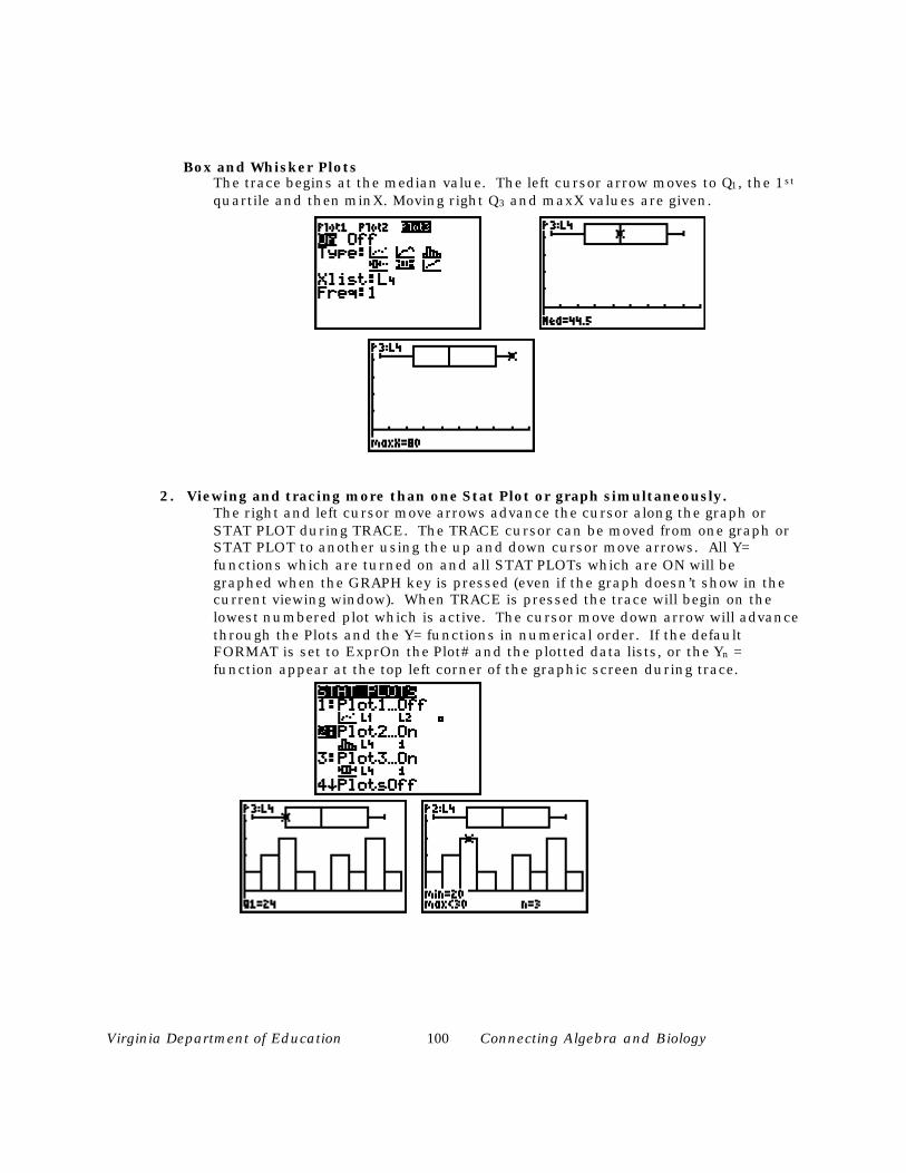
Virginia Department of Education 100 Connecting Algebra and Biology
Box and Whisker PlotsThe trace begins at the median value. The left cursor arrow moves to Q1, the 1st
quartile and then minX. Moving right Q3 and maxX values are given.
2. Viewing and tracing more than one Stat Plot or graph simultaneously.The right and left cursor move arrows advance the cursor along the graph orSTAT PLOT during TRACE. The TRACE cursor can be moved from one graph orSTAT PLOT to another using the up and down cursor move arrows. All Y=functions which are turned on and all STAT PLOTs which are ON will begraphed when the GRAPH key is pressed (even if the graph doesn’t show in thecurrent viewing window). When TRACE is pressed the trace will begin on thelowest numbered plot which is active. The cursor move down arrow will advancethrough the Plots and the Y= functions in numerical order. If the defaultFORMAT is set to ExprOn the Plot# and the plotted data lists, or the Yn =function appear at the top left corner of the graphic screen during trace.
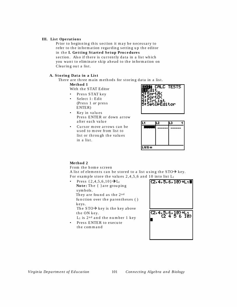
Virginia Department of Education 101 Connecting Algebra and Biology
III. List OperationsPrior to beginning this section it may be necessary torefer to the information regarding setting up the editorin the I. Getting Started Setup Proceduressection. Also if there is currently data in a list whichyou want to eliminate skip ahead to the information onClearing out a list.
A. Storing Data in a List There are three main methods for storing data in a list. Method 1
With the STAT Editor
• Press STAT key• Select 1: Edit
(Press 1 or press ENTER)
• Key in valuesPress ENTER or down arrowafter each value
• Cursor move arrows can beused to move from list tolist or through the valuesin a list.
Method 2From the home screenA list of elements can be stored to a list using the STOà key.For example store the values 2,4,5,6 and 10 into list L1
• Press { 2,4,5,6,10} ààL1
Note: The { } are grouping symbols. They are found as the 2nd
function over the parentheses ( ) keys.
The STOà key is the key above the ON key.
L1 is 2nd and the number 1 key• Press ENTER to execute
the command
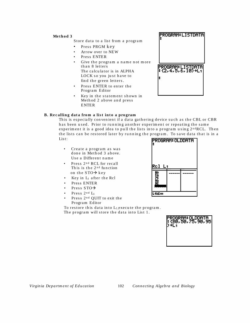
Virginia Department of Education 102 Connecting Algebra and Biology
Method 3Store data to a list from a program
• Press PRGM key• Arrow over to NEW• Press ENTER• Give the program a name not more
than 8 lettersThe calculator is in ALPHALOCK so you just have tofind the green letters.
• Press ENTER to enter theProgram Editor
• Key in the statement shown inMethod 2 above and pressENTER
B. Recalling data from a list into a programThis is especially convenient if a data gathering device such as the CBL or CBRhas been used. Prior to running another experiment or repeating the sameexperiment it is a good idea to pull the lists into a program using 2ndRCL. Thenthe lists can be restored later by running the program. To save data that is in aList:
• Create a program as wasdone in Method 3 above.Use a Different name
• Press 2nd RCL for recall This is the 2nd function
on the STOà key• Key in L1 after the Rcl• Press ENTER• Press STOà• Press 2nd L1
• Press 2nd QUIT to exit theProgram Editor
To restore this data into L1,execute the program. The program will store the data into List 1.
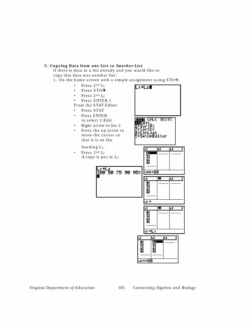
Virginia Department of Education 103 Connecting Algebra and Biology
C. Copying Data from one List to Another ListIf there is data in a list already and you would like tocopy this data into another list:1. On the home screen with a simple assignment using STOà.
• Press 2nd L1
• Press STOàà• Press 2nd L2
• Press ENTER 1From the STAT Editor• Press STAT• Press ENTER
to select 1:Edit• Right arrow to list 2• Press the up arrow to
move the cursor so that it is on the
heading L2.
• Press 2nd L1
A copy is put in L2
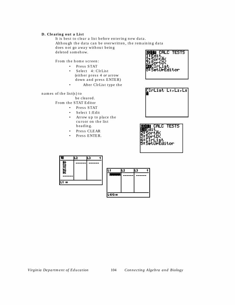
Virginia Department of Education 104 Connecting Algebra and Biology
D. Clearing out a ListIt is best to clear a list before entering new data.Although the data can be overwritten, the remaining datadoes not go away without being
deleted somehow.
From the home screen:
• Press STAT• Select 4: ClrList
(either press 4 or arrow down and press ENTER)
• After ClrList type the
names of the list(s) to be cleared.
From the STAT Editor• Press STAT• Select 1:Edit• Arrow up to place the
cursor on the listheading.
• Press CLEAR• Press ENTER.
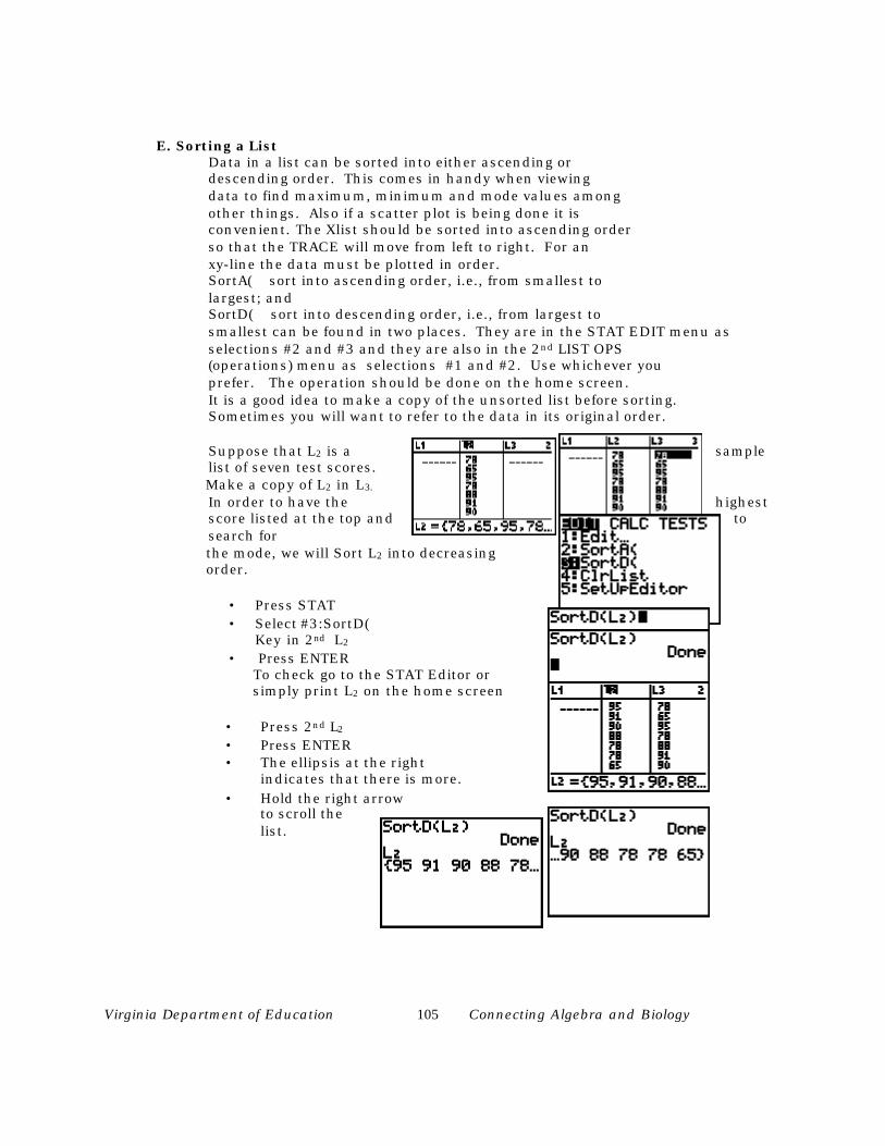
Virginia Department of Education 105 Connecting Algebra and Biology
E. Sorting a ListData in a list can be sorted into either ascending ordescending order. This comes in handy when viewing
data to find maximum, minimum and mode values among other things. Also if a scatter plot is being done it is convenient. The Xlist should be sorted into ascending order so that the TRACE will move from left to right. For an xy-line the data must be plotted in order.
SortA( sort into ascending order, i.e., from smallest to largest; and SortD( sort into descending order, i.e., from largest to
smallest can be found in two places. They are in the STAT EDIT menu asselections #2 and #3 and they are also in the 2nd LIST OPS(operations) menu as selections #1 and #2. Use whichever youprefer. The operation should be done on the home screen.It is a good idea to make a copy of the unsorted list before sorting.Sometimes you will want to refer to the data in its original order.
Suppose that L2 is a samplelist of seven test scores.
Make a copy of L2 in L3.
In order to have the highestscore listed at the top and tosearch for
the mode, we will Sort L2 into decreasing order.
• Press STAT• Select #3:SortD(
Key in 2nd L2
• Press ENTER To check go to the STAT Editor or
simply print L2 on the home screen
• Press 2nd L2
• Press ENTER • The ellipsis at the right
indicates that there is more.
• Hold the right arrow to scroll the list.
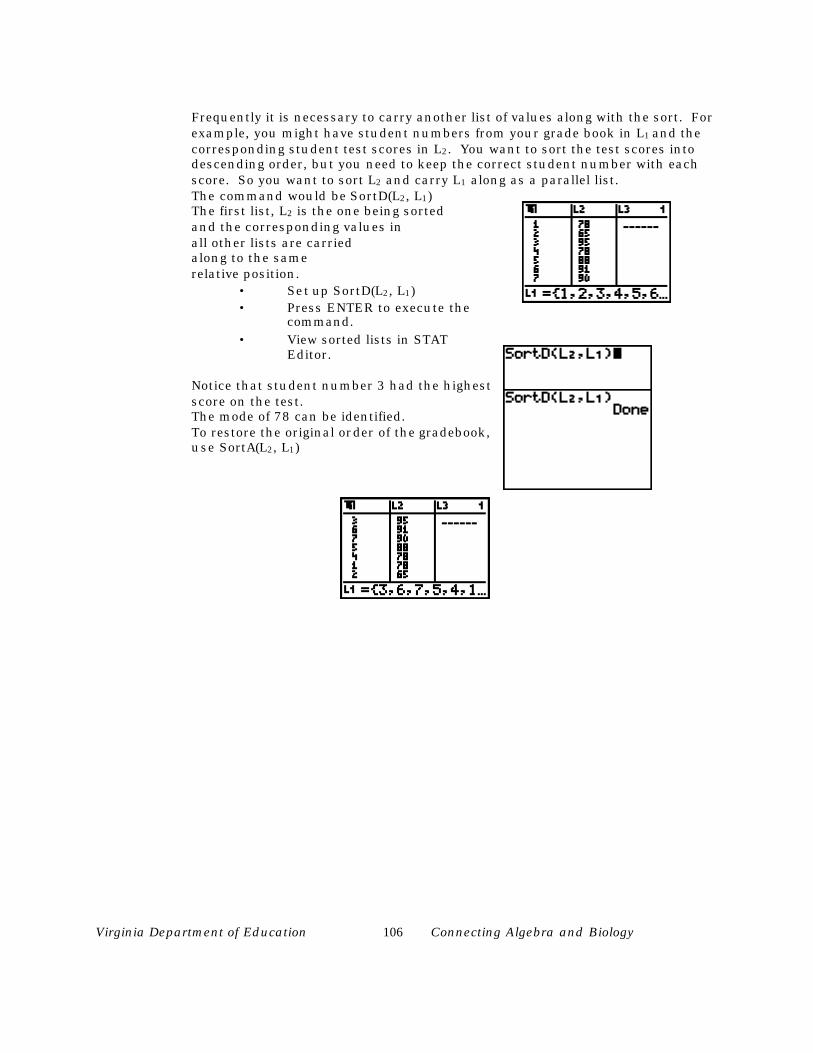
Virginia Department of Education 106 Connecting Algebra and Biology
Frequently it is necessary to carry another list of values along with the sort. Forexample, you might have student numbers from your grade book in L1 and thecorresponding student test scores in L2. You want to sort the test scores intodescending order, but you need to keep the correct student number with eachscore. So you want to sort L2 and carry L1 along as a parallel list.The command would be SortD(L2, L1)The first list, L2 is the one being sortedand the corresponding values in
all other lists are carried along to the same relative position.
• Set up SortD(L2, L1)• Press ENTER to execute the
command.
• View sorted lists in STATEditor.
Notice that student number 3 had the highest score on the test.
The mode of 78 can be identified. To restore the original order of the gradebook,
use SortA(L2, L1)
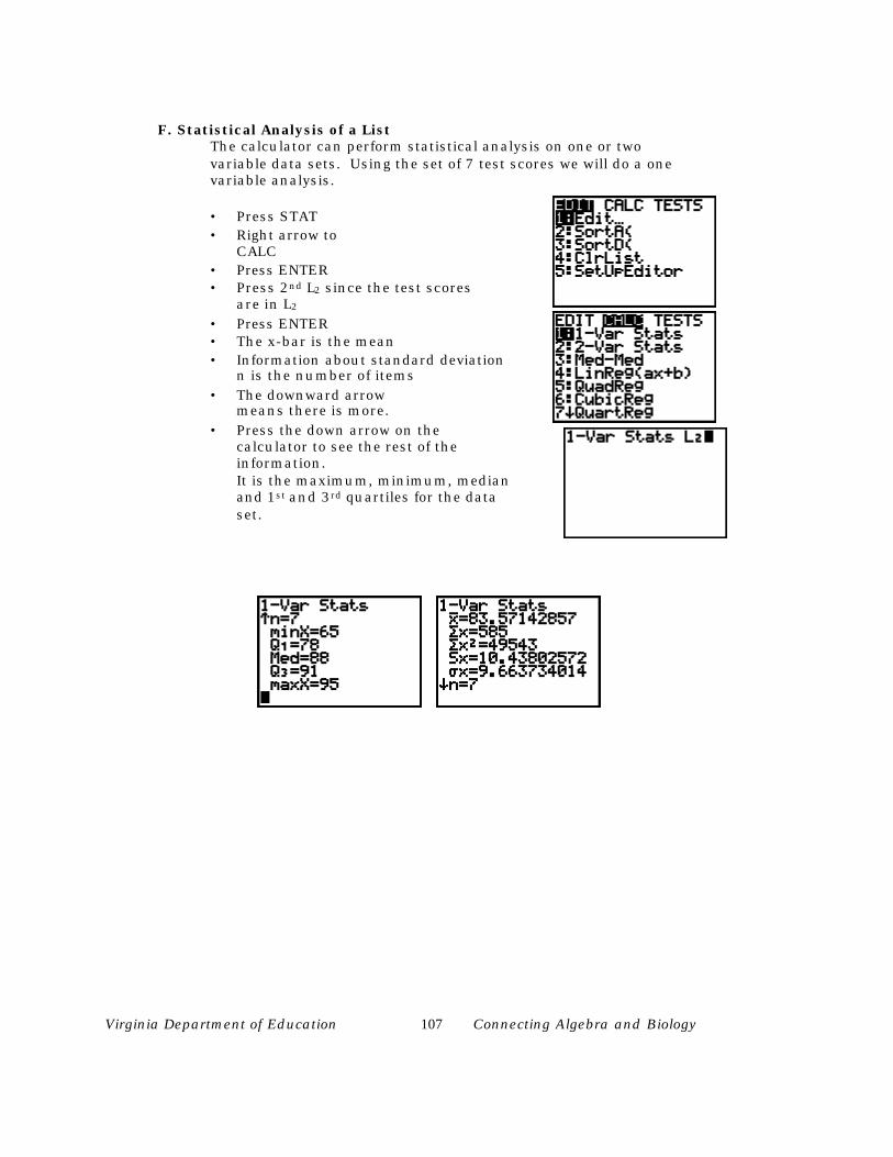
Virginia Department of Education 107 Connecting Algebra and Biology
F. Statistical Analysis of a ListThe calculator can perform statistical analysis on one or twovariable data sets. Using the set of 7 test scores we will do a onevariable analysis.
• Press STAT• Right arrow to
CALC• Press ENTER• Press 2nd L2 since the test scores
are in L2
• Press ENTER• The x-bar is the mean• Information about standard deviation
n is the number of items
• The downward arrow means there is more.
• Press the down arrow on thecalculator to see the rest of theinformation.It is the maximum, minimum, medianand 1st and 3rd quartiles for the dataset.
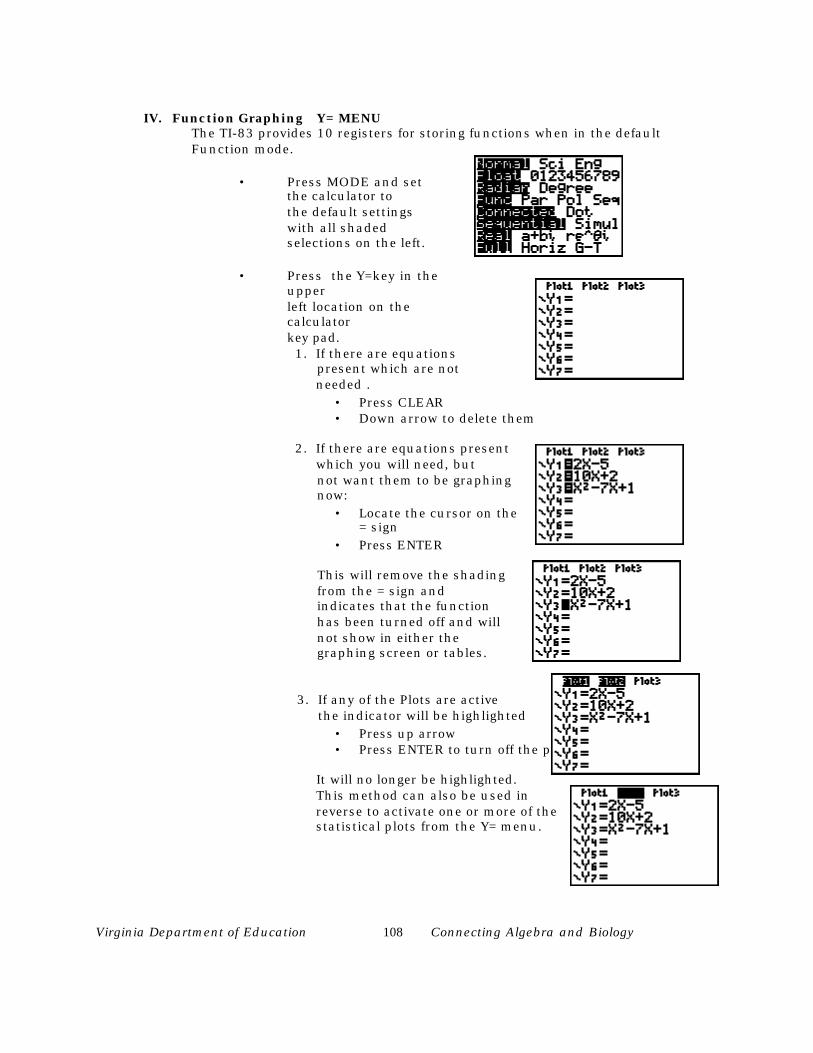
Virginia Department of Education 108 Connecting Algebra and Biology
IV. Function Graphing Y= MENUThe TI-83 provides 10 registers for storing functions when in the defaultFunction mode.
• Press MODE and set the calculator to
the default settings with all shaded
selections on the left.
• Press the Y=key in the upper
left location on the calculator
key pad. 1. If there are equations
present which are not needed .
• Press CLEAR• Down arrow to delete them
2. If there are equations present which you will need, but not want them to be graphing now:
• Locate the cursor on the= sign
• Press ENTER
This will remove the shading from the = sign and indicates that the function has been turned off and will not show in either the graphing screen or tables.
3. If any of the Plots are active the indicator will be highlighted
• Press up arrow• Press ENTER to turn off the plot
It will no longer be highlighted. This method can also be used in reverse to activate one or more of the statistical plots from the Y= menu.
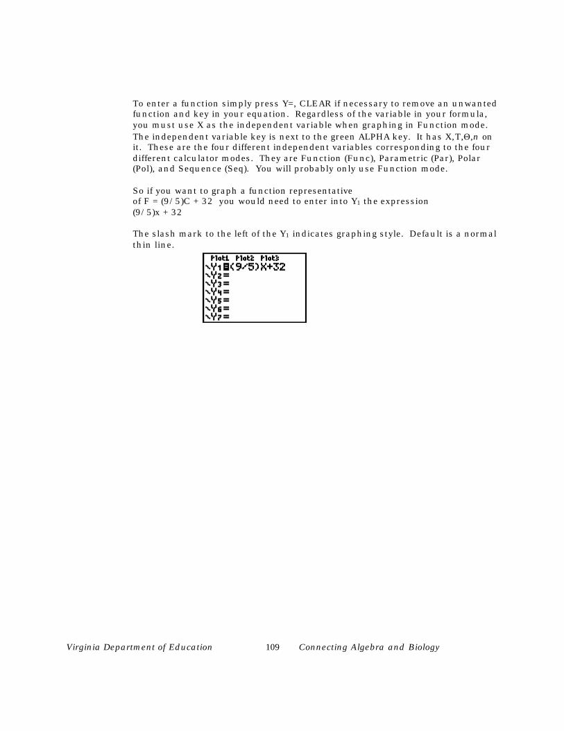
Virginia Department of Education 109 Connecting Algebra and Biology
To enter a function simply press Y=, CLEAR if necessary to remove an unwantedfunction and key in your equation. Regardless of the variable in your formula,you must use X as the independent variable when graphing in Function mode.The independent variable key is next to the green ALPHA key. It has X,T,Θ,n onit. These are the four different independent variables corresponding to the fourdifferent calculator modes. They are Function (Func), Parametric (Par), Polar(Pol), and Sequence (Seq). You will probably only use Function mode.
So if you want to graph a function representativeof F = (9/5)C + 32 you would need to enter into Y1 the expression(9/5)x + 32
The slash mark to the left of the Y1 indicates graphing style. Default is a normalthin line.

Virginia Department of Education 110 Connecting Algebra and Biology
V. Linking
A. Calculator to Calculator
The black link cable supplied with the calculator allows you to transfer datafrom one calculator to another. It is possible to transfer programs, lists,equations, etc., or even make one calculator an exact copy of the other by doinga back up.The process is described in the TI-83 users manual. Briefly it is as follows.
1. Press the link cable firmly into the link port in the bottom ofeach calculator. Push hard. Sometimes it does not go in allthe way at first.
2. Turn on both calculators.3. On the calculator which will be
receiving the data:
• Press 2nd LINK (it is over the independent
variable key (X,T,Θ,n)• Right arrow to RECEIVE• Press ENTER• Waiting…
4. On the sending calculator• Press 2nd LINK• Press the number of your
choice
• Press ENTER next to any item which you want to send. This will put a box next to that item indicating that it is selected.• Arrow over to TRANSMIT• Press ENTER
5. If the receiving calculator already has data in the named item whichis being sent the calculator will offer the options of
Rename, Overwrite, Omit, or Quit.

Virginia Department of Education 111 Connecting Algebra and Biology
B. Calculator to CBL Linking
The calculator is linked to the CBL with the same cord as is used for thecalculator to calculator linking. The link port for the CBL to calculatorlink is located at the bottom of the CBL in a place similar to where it ison the calculator. Both devices must be turned on. A program isnecessary to either send commands to the CBL or to receive data fromthe CBL into the calculator.
C. Calculator to Computer Linking
The TI-GRAPH LINK made by Texas Instruments is sold through alleducational dealers who carry TI products as well as at some local stores.If purchased from an educational dealer you will receive one link cablewith adapters which allow you to connect to either a MacIntosh or PCthrough the serial port. A manual and software are provided for bothoperating systems and for all of the Texas Instruments link-ablecalculators. The software is self-installing.
Advantages include:1. Programs and data can be saved on the computer or floppy so that there will be enough memory in the calculator for other activities.2. Special programs distributed by vendors along with activity workbooks can be loaded into the calculator.3. Graphs, data lists and other calculator screens can be printed by the teacher for activities.4. Graphs, data lists and other calculator screens can be printed by students for inclusion in lab reports.5. Data can be loaded into the computer for analysis with other software.6. Programs can be sent to the calculator after being downloaded from Web sites.
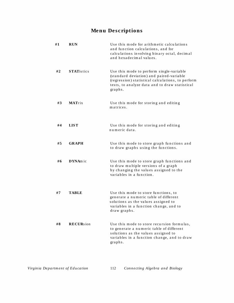
Virginia Department of Education 112 Connecting Algebra and Biology
Menu Descriptions
#1 RUN Use this mode for arithmetic calculations and function calculations, and for calculations involving binary octal, decimal and hexadecimal values.
#2 STATistics Use this mode to perform single-variable(standard deviation) and paired-variable(regression) statistical calculations, to performtests, to analyze data and to draw statisticalgraphs.
#3 MATrix Use this mode for storing and editing matrices.
#4 LIST Use this mode for storing and editing numeric data.
#5 GRAPH Use this mode to store graph functions and to draw graphs using the functions.
#6 DYNAmic Use this mode to store graph functions and to draw multiple versions of a graph by changing the values assigned to the
variables in a function.
#7 TABLE Use this mode to store functions, to generate a numeric table of different solutions as the values assigned to
variables in a function change, and todraw graphs.
#8 RECURsion Use this mode to store recursion formulas,to generate a numeric table of differentsolutions as the values assigned tovariables in a function change, and to drawgraphs.

Virginia Department of Education 113 Connecting Algebra and Biology
#9 CONICS Use this mode to draw graphs of implicitfunctions.
A EQUAtion Use this mode to solve linear equationswith two through six unknowns, quadraticequations, and cubic equations.
B PRoGraM Use this mode to store programs in theprogram area and to run programs.
C Time Value Use this mode to perform financialcalculations of Money and to draw cashflow and other types of graphs.
D LINK Use this mode to transfer memory contentsor back-up data to another unit.
E CONTrast Use this mode to adjust the color contrast of the display.
F MEMory Use this mode to check how much memoryis used and remaining, to delete data frommemory, and to initialize (reset) thecalculator.
Virginia Department of Education 114 Connecting Algebra and Biology
Measurement and Conversion
This activity is an introduction to the Casio 9850G-Plus. It serves as anoverview of some of the capabilities of this graphing calculator.
Materials
ü Casio 9850G-Plus graphing calculatorü Measuring tape (English)ü Measuring tape (Metric)ü Class data worksheet
Procedure
Get a partner.
You and your partner should use the appropriate measuring tapes tomeasure each other’s heights in both inches and centimeters.
Each person should record his/her height data on a group chart in the frontof the room.
Each person should copy the class data onto the attached class dataworksheet.
Follow the calculator procedure.
Calculator Procedure
NOTE: For the purpose of showing directions in this section, a set of data will be provided; your data will vary slightly from the sample data but
should show similar trends.
List 1: 65, 61, 57, 69, 63, 71, 68 inches
List 2: 165, 154, 145, 175, 160, 180, 173 centimeters
Virginia Department of Education 115 Connecting Algebra and Biology
1. To Clear Lists and FunctionsIn order to manipulate the class data, any existing data within the calculator
will have to be cleared.
A. To clear existing equations:
Go to the GRAPH mode (#5) on the calculator.
Select F2 (DEL), select F1 (YES). The second command hereallows you a second chance to say whether you really want to
delete the highlighted equation or not.
Press the down arrow key in order to highlight any other existingequations. Once each existing equation has been highlighted,select F2 (DEL), then select F1 (YES).
B. To clear data in existing lists:
Go to the STAT mode (#2) on the calculator.
Press the F6 (ω) key until you see the DEL-A option above the F4Function key.
Press the up arrow key in order to highlight the words “List 1”.Press F4 (DEL-A). All data in List 1 should now be highlighted. Press F1(YES) to finish the job of deleting List 1.
Use the right arrow key in order to highlight any other Lists thatcontain data. Select F4 (DEL-A), then select F1 (YES). It is important tomake sure that you initially highlight the name of the list at the top ofeach column and not the first piece of data in order to delete all data thatis contained in that list.
2. Now that the graphing calculator is cleared of equations and lists, it’s time to enter the New Data.
Go to the STAT Mode (#2) on the calculator. The cursor should be in thefirst position of List 1.
Enter the inch data into List 1 by keying in the digits of your firstmeasurement. Check your entry at the bottom of your screen on the left-hand side above the option labels before hitting the EXE key. Pressingthe EXE key will automatically move you to the next line ready for moredata input.

Virginia Department of Education 116 Connecting Algebra and Biology
Any data that has been input incorrectly can be easily fixed.
If the mistake is discovered before the EXE key is pressed, then usethe left arrow key to place the cursor under the incorrect digit(s) andthen press the DEL key. Now input the correct data and press theEXE key.
If the mistake is discovered after the EXE key is pressed, then usethe up arrow key to highlight the incorrect piece of data and simplytype in the corrected data and press the EXE key. The new data willnow appear.
A piece of data that has been inputted and is no longer needed inthat space will require a different set of key strokes. First of all, usethe up or down arrow key in order to highlight the extraneous pieceof data. Secondly, select F6 (ω). Lastly, select F3(DEL). The datashould now be gone. The rest of the data in the list will move up thecolumn accordingly.
Any data that has been accidentally omitted can be inserted in usingthese steps. Use the up or down arrow key to highlight the place
where the missing data belongs. Select F6 (ω), the select F5 (INS).Input the missing piece of data now. Press the EXE key. The rest ofthe data in the list will move down the column accordingly.
Once all of the inch data has been entered, use the right arrow key tomove over to List 2, position one. Enter the centimeter data into List 2.
3. To organize the data within the lists according to ascending value
Go to the STAT Mode (#2) on your calculator.
Press F6 (ω).
Select F1 (SRT-A). Sort the data in List 1.
At this point, the calculator is asking, “How Many Lists? (H)”. Press 1,and then EXE to sort one list.
The calculator is now asking, “Select List (L)”. Press 1, and then EXE.The data in List 1 should now be in ascending order.

Virginia Department of Education 117 Connecting Algebra and Biology
4. Analyze the data.
Go to the STAT Mode (#2) on the calculator.
Press F2 (CALC). This will bring up another row of options above the functionkeys.
Press F6 (SET). On the screen now is a listing of where the statistical data forthe calculation is located. For the purposes of this exercise, we only need to beconcerned with the first item that is already highlighted, “1Var XList : List1”.This is specifying List1 to be the list where single-variable statistic x-values(XList) are located. To change the specificity of the list to List2, List3, List4,List5, or List6, use the function keys that correlate with the option labels at thebottom of the screen. Now, make sure that for this exercise List1 has beenspecified.
Select the EXIT key. This moves back to the previous screen.
Select F1 (1VAR). This will give an analysis of the data in List1. Use the downarrow key to scroll down the screen and view the items that run off the bottom ofthe screen. The following describes the meaning of each of the parameters:
² …………. Mean of data ∑x ………… Sum of data
∑xâ ……….. Sum of squares xσÌ ………… Population standard deviation
xσÌý ………. Sample standard deviationÌ …………… Number of data itemsminx ……… MinimumQ1 ………… First QuartileMed ………. Median
²-xσÌ ……. Data mean – Population standard deviation²+xσÌ ……. Data mean + Population standard deviationQ3 ………… Third QuartilemaxX …….. Maximum
Mod ………. Mode

Virginia Department of Education 118 Connecting Algebra and Biology
5. Data can be analyzed in the RUN Mode (#1) as well.
Go to the RUN Mode (#1). This is a section of the calculator where basicfunctions (i.e. - addition, subtraction, multiplication, and division) can beaccomplished, as well as so much more.
Select the OPTN key. A row of icons appears at the bottom of the screen andabove the six function keys.
Select F1 (LIST). Another row of icons now appears. Select F6 (ω) to reveal moreicons.
At this point we could find out the Median of the data in List 1. Select F4 (Med).Select the EXIT key to go back to the previous screen of option icons. Select F1(LIST). Select F1 (List) again. Press the number 1 to denote finding the medianof List 1. Press the EXE key to execute the command. The answer shouldappear on the right-hand side of the screen.
The mean of List 1 could be found very similarly. Select F6 (ω). Select F3(Mean). Press the EXIT key. Select F1 (LIST). Select F1 (List). Press thenumber 1 and then the EXE key.
At this point, clear the screen by pressing the AC/ON key. Repeatedly press theEXIT key to clear the option icons at the bottom of the screen.
To find out how many pieces of data are in a list, press the OPTN key. Select F1(LIST). Select F3 (Dim). Select F1 (List). Press the number 1 and then the EXEkey.
To find the differences between successive terms in a list, in other wordscreating a delta list, do the following: Press F6 (ω), Press F6 (ω) again, Press F5(∆), Press the number 1 to denote List 1 and then the EXE key. Use the up anddown arrow keys to scroll up and down the delta list.
This delta list can even be stored in a different list as part of the STAT Mode(#2). Select F5 (∆). Press the number 1. Now before pressing the EXE key,press the Ü (send) key located above the AC/ON key. This is telling thecalculator to send the answer somewhere else. At this point, we need to type inwhere the answer should be sent. Press the EXIT key. Select F1 (LIST). SelectF1 (List). Press the number 3 to send the answer into List 3. Press the EXEkey. A message on the right-hand side of the screen says, “Done”. To see theanswer in List 3, press the MENU key. Go to STAT Mode (#2). Use the arrowkeys to scroll up and down List 3.

Virginia Department of Education 119 Connecting Algebra and Biology
To square the inches from List 1, go back to the Main Menu. Press the MENUkey. Select the RUN Mode (#1). Press the OPTN key. Select F1 (LIST). SelectF1 (List). Press the number 1. Press the x² key located to the right of the redALPHA key. Now select the Ü (send) key above the AC/ON key. Press F1 (List).Press the number 4 to send the answers to List 4. Press the EXE key. To seethe answers, press the MENU key. Select the STAT Mode (#2) key.
6. To look at the domain of the values in a list using a Box Plot:
Select STAT Mode (#2).
Press F1 (GRPH). This takes us into the Graph options.
Press F6 (SET). This will allow us to set up our Box Plot graph.
Use the down arrow key to highlight the Graph Type. Press F6 (ω). Select F2(Box). This will set the graph as a Box Plot.
Use the down arrow key to highlight the XList. Select F1 (List1). The Box Plot isto be drawn from the data in List 1
Use the down arrow key to highlight the Frequency. Select F1 (1).
Use the down arrow key to highlight the Graph Color. Choose any of the threecolors. Press F1 (Blue), F2 (Orng), or F3 (Grn).
Use the down arrow key to highlight the Outliers. Press F1 (On) to turn theoutliers on.
Press the EXE key to complete the set-up of our Box Plot.
Press F4 (SEL). This goes into another screen that gives the option of viewing upto three graphs at once. At this point, we only want to view StatGraph1. Usethe arrow keys to highlight StatGraph1. Press F1 (On). Highlight StatGraph2.Press F2 (Off). Highlight StatGraph 3. Press F2 (Off). Press F6 (DRAW) to drawour box plot.
Trace along the box plot to read the quartile data. Select the SHIFT key, thenpress the F1 (TRCE) key. Press the left and right arrow keys to read the quartiledata.
Virginia Department of Education 120 Connecting Algebra and Biology
7. To establish a histogram of the List 1 data, height of the class in inches:
From the Main Menu, choose STAT Mode (#2).
Press F6 (SET). Highlight the Graph Type. Press the F6 (ω) key. Select F1(Hist). Highlight the XList. Select F1 (List 1) to pull the data from List 1 tocreate the histogram. Highlight the Frequency. Select F1 (1). Highlight GraphColor. Choose any of the three colors. Press the EXE key.
Press F4 (SEL). Make sure only StatGraph1 is ON.
Select F6 (DRAW).
This is the Set Interval screen. “Start” refers to the histogram start point.“Pitch” refers to the bar spacing or the scale unit. The calculator canautomatically choose these settings or you can customize them. For thepurposes of this exercise, leave the Start setting alone, but change the pitch to3. Do this by highlighting the pitch setting. Press the number 3. Press the EXEkey. The EXE key must be pressed at this point, or the calculator willautomatically revert the pitch setting back to what it had wanted to set it at.Press F6 (DRAW).
Press the SHIFT key followed by F1 (TRCE). Use the left and right arrow keys toobtain values represented. Notice the height intervals defined by each portion ofthe bar graph; notice the number of people whose height fell within that intervalis defined under “f”.

Virginia Department of Education 121 Connecting Algebra and Biology
To practice the skills outlined in this lesson, examine the data in List 2, height incentimeters. It was not sorted with List 1 because it was not included in the sortcommand. Sort the data and answer the following questions using the techniquespresented in this exercise.
1. From the sorted list, what is the shortest height in centimeters?
2. From the sorted list, what is the tallest height in centimeters?
3. What is the sum of all the heights in List 2?
4. What is the sum of all the heights squared in List 2? What is the unit?
5. What is the standard deviation of List 2?
6. What is the mean height of List 2?
7. What is the median height of List 2?
8. Set up a box and whiskers plot of List 2. What is the lower quartile? What is the upperquartile?
9. What is the inner quartile difference in heights (Q3 – Q1)?
10. Construct a histogram of the data in List 2. Allow the calculator to set a pitch, as well as set a pitch of your choice. What is the most common height interval in the class?

Virginia Department of Education 122 Connecting Algebra and Biology
8. To establish a direct or inverse relationship between the measurements in inches andin centimeters,
A. Gather the data together in a scatter plot.
Go to the STAT Mode (#2) on the calculator.
Press F1 (GRPH). Press F6 (SET).
Use the down arrow key to highlight Graph Type. Select F1(Scat). Enter the appropriate list values as follows:
XList : List 1YList : List 2Frequency : 1Mark Type : Choose oneGraph Color : Choose one
Press EXE when all of the previous information has been entered in.
Select F4 (SEL). Make sure only StatGraph1 is on. Select F6 (DRAW).
B. Establish a regression equation which best fits experimental data.
The data appears to be linear by its scatter plot; therefore select F1 (x).The screen now shows the coefficients of a and b in linear regressionanalysis, y = ax + b; a is the slope of the line, b is the y intercept. Thelower case r is the regression coefficient, which indicates how close thescattered points fit the regression line. Values closer to one areconsidered a good fit! This data reflects the direct relationship betweenmeasurements made in metric and English. The slope of the resultingline will show the equivalency between centimeters and inches andshould be close to 2.54; 2.54 centimeters is approximately equal to 1.00inch.
Press F5 (COPY). This will transfer the equation directly to theGraph Function Y = screen. Press EXE. Press F6 (DRAW). Theline created from the equation is now drawn on the scatter plot.
Virginia Department of Education 123 Connecting Algebra and Biology
Understand the Casio Data Analyzer (EA-100) Keyboard
The keyboard has eight function keys and five additional shifted functions.
Description of Eight EA-100 Keys:
ON/OFF Turns Data Analyzer on and off.
SHIFT Used to access the functions printed above the keys in gold. The wordSHIFT appears in the upper right-hand corner of the screen.
MODE Shifts the Data Analyzer between the multimeter mode (the wordMULTIMETER appears in the lower left-hand corner of the screenwhen in this mode) and the communications mode; most oftenyou want to be in the communications mode.
TRIGGER Each press of this key while the Data Analyzer is in the READYstate takes a data sample. (The word READY appears on the left-hand side of the screen.)
CH-View Depends on the mode (e.g., changes which channel’s data aredisplayed). See pages 6 and 7 of the Data Analyzer manual.
• Communication• Multimeter• Internal• Data-Log Mode
INTERNAL Tells you the current voltage remaining in the Data Analyzer’s batteries.
DataLOG Allows you to scroll through data stored in the Data Analyzer.In the multimeter mode, this key changes the unit of
measurement for the displayed channel.
HALT Serves several functions (e.g., halts a sampling operation). Seepage 7 of the Data Analyzer manual.

Virginia Department of Education 124 Connecting Algebra and Biology
Description of Five Shift Functions (printed in gold above the keys):
SETUP Press SHIFT + MODE to enter the SETUP mode to usethe Data Analyzer as a stand-alone device to sample data(no program is needed for a calculator).
XMIT-9800 Sends data to a CFX-9800G calculator.
RESTART Pressing SHIFT + HALT clears any existing sampled data andreturns the Data Analyzer to the READY state to begin again.
NEXT In the Setup Mode and the DataLOG Mode, this key gives thenext choice in a sequence or the next data value.
ENTER The Trigger key serves as an “enter” key when selecting values forthe Setup mode.

Virginia Department of Education 125 Connecting Algebra and Biology
Casio Program-Link (FA-122)
Transferring files from the graphing calculator to the computer:
1. Install the Casio Program-Link into the computer’s hard drive. To retrieve it, go toPrograms on the hard drive.
2. Connect the communication cable to the computer’s COM1 or COM2 port.
3. Turn the calculator ON. Make sure to connect the communication cable from thecomputer to the calculator!
4. On the computer select LINK on the menu control bar. Scroll down to highlightReceive.
5. On the graphing calculator, go to LINK Mode (letter D). Press F1 (TRAN). Press F1(SEL). Highlight the data item you want to send. Press F6 (TRAN). Press F1 (YES).The data transfer should start at this time, with its progress indicated by a dialog boxon the computer screen. The message, “Transmit ERROR!” appears on the calculatorscreen if the computer is not set up to receive data.
6. When data transfer is complete, a new catalog window appears on the computer screen.Save the data as a file. On the computer, select FILE on the menu control bar. Scrolldown to highlight Save or Save As. Specify a file name and click OK to save it as acatalog file.
7. Double check the following items whenever data transfer is not performed correctly:
• Check for proper connection of the communication cable.
• Check that the port was correctly selected on the computer. Do this by selectingLINK on the menu control bar, and then scrolling down to highlightCommunications.
Virginia Department of Education 126 Connecting Algebra and Biology
Transferring files from the computer to the calculator:
1. Install the Casio Program-Link into your computer’s hard drive. To retrieve it, go toPrograms on the hard drive.
2. Connect the communication cable to the computer’s COM1 or COM2 port.
3. Turn the calculator ON. Make sure to connect the communication cable from thecomputer to the calculator!
4. On the computer select FILE on the menu control bar. Scroll down to highlight OPEN.A dialog box should appear. This dialog box can be used to specify a file name and alsoto specify a drive and directory.
5. Click on a group and item to select it for transfer.
6. Go to LINK mode (letter D) on the graphing calculator. Press F2 (RECV).
7. On the computer select LINK on the menu control bar. Scroll down to highlightTRANSMIT. Double check to make sure that both units are set up correctly for datatransfer and then click OK. Data transfer starts at this time, with its progress indicatedby a dialog box on the computer screen. If a received file has a name of a file alreadystored in calculator memory, a dialog box appears asking if you want to overwrite theexisting file. Select YES or NO in response to the dialog message. The message“Transmit ERROR” appears if the calculator is not set up to receive data.
8. When data transfer is complete, the dialog box closes.
9. Double check the following items whenever data transfer is not performed correctly:
• Check for proper connection of the communication cable.
• Check that the port was correctly selected on the computer. Do this by selectingLINK on the menu control bar, and then scrolling down to highlightCommunications.

Virginia Department of Education 127 Connecting Algebra and Biology
Capturing a screen to your computer:
1. Install the Casio Program-Link into your computer’s hard drive. To retrieve it, go toPrograms on the hard drive.
2. Connect the communication cable to the computer’s COM1 or COM2 port.
3. Turn the calculator ON. Make sure to connect the communication cable from thecomputer to the calculator!
4. Go to LINK Mode (letter D) on your calculator. Press F6 (IMGE ). Press F2 (MONO).Perform the necessary operations on the calculator to produce the desired screen.
5. On the computer, select LINK on the menu control bar. Scroll down to highlightScreen Capture.
6. On the graphing calculator, press the F↔↔ D key located above the number 8. The datatransfer should begin now, with its progress indicated by a dialog box on the computerscreen.
7. After the transfer is complete, the screen data appears on the computer screen.
8. Save the data in a file. Select FILE on the control menu bar. Scroll down to highlightSAVE or SAVE AS. Specify a file name and click OK to save it.
9. While the image is on the display, select FILE on the control menu bar. Scroll down tohighlight PRINT. Specify the printer, print options, number of copies, and enlargementfactors, and then start the printing. The preview function can be used to display animage of the printout on the screen.

Virginia Department of Education 128 Connecting Algebra and Biology