Conjugate-normal matrices: A survey

H. Faßbender a, Kh. D. Ikramov b,∗,1

aInstitut Computational Mathematics, TU Braunschweig, Pockelsstr. 14, D-38023Braunschweig, Germany.

bFaculty of Computational Mathematics and Cybernetics, Moscow StateUniversity, 119992 Moscow, Russia.

Abstract

Conjugate-normal matrices play the same important role in the theory of unitarycongruence as the conventional normal matrices do with respect to unitary similari-ties. However, unlike the latter, the properties of conjugate-normal matrices are notwidely known. Motivated by this fact, we give a survey of the properties of thesematrices. In particular, a list of more than forty conditions is given, each of whichis equivalent to A being conjugate-normal.

Key words: consimilarity, unitary congruence, coneigenvalue, coninvariantsubspace, conjugate-normal matrix, Youla theorem, concommutation2000 MSC: 15A21

1 Introduction

As justly noted in (HJ1, Section 2.5), the class of normal matrices is importantthroughout matrix analysis. It is especially important in matters related tosimilarity transformations and, even more specifically, to unitary similaritytransformations. Such significant matrix classes as Hermitian, skew-Hermitian,and unitary matrices are subclasses of normal matrices.

The importance of normal matrices explains the appearance of the survey(GJSW) in 1987. It contains 70 conditions, each equivalent to the original

∗ corresponding authorEmail addresses: h.fassbender@tu-bs.de (H. Faßbender),

ikramov@cs.msu.su (Kh. D. Ikramov).1 The work of this author has been supported by the Deutsche Forschungsgemein-schaft.

Preprint submitted to Elsevier 30 November 2007

definition of normality, i.e., to the relation

AA∗ = A∗A. (1)

One decade later, about twenty additional criteria for normality were presentedin (EI). For brevity, we refer to these two papers as the GJSW list and EI list,respectively.

If we are dealing with unitary congruences rather than unitary similarities,then normality is no longer a useful property, because it is not preserved byunitary congruence transformations. Is there a matrix class that can replacenormal matrices in this new context?

The answer is yes, and the required matrix class are the so-called conjugate-normal matrices.

Definition 1 A matrix A ∈ Mn(C) is said to be conjugate-normal if

AA∗ = A∗A. (2)

In particular, complex symmetric, skew-symmetric, and unitary matrices arespecial subclasses of conjugate-normal matrices.

It seems that the term ’conjugate-normal matrices’ was first introduced in(VHV), that is, 35 years ago. However, despite this respectable age, the prop-erties of these matrices are not known as broadly as they, in our opinion,deserve to be.

Our intention in this paper is to give a survey of properties of conjugate-normalmatrices. Moreover, we give a list of conditions equivalent to definition (2),which thus may be taken as condition 0 in this list. Citing (GJSW), ’since weknow of no similar list, our hope is that this will be generally useful to thematrix community.’

The paper is organized as follows. The necessary preliminary material is pre-sented in Section 2. It includes a discussion of distinctions between the theoriesof two matrix relations: similarity and consimilarity. Section 3 deals with el-ementary properties of conjugate-normal matrices and their canonical formswith respect to unitary congruences. The next two sections follow the patterngiven in (GJSW): first, about forty condition each equivalent to (2) are given,then brief proofs of or comments to these conditions are given in Section 5.Section 6 contains our concluding remarks.

We use the following notation. If A ∈ Mn(C), then AT , A, A∗ and A+ are thetranspose, the entrywise conjugate, the Hermitian adjoint, and the Moore-

2

Penrose inverse of A, respectively. The singular values of A are denoted bys1 ≥ s2 ≥ . . . ≥ sn, its spectral radius by ρ(A), and its spectrum by λ(A).The symbol Ck(A) stands for the kth compound matrix of A, (MM, p. 16).By Nn and CN n, we denote the classes of n×n normal and conjugate-normalmatrices, respectively. The subscript is omitted if the order of A is clear fromthe context or not relevant. Depending on the context, the symbol || · ||2 isused for the 2-norm of a vector or the spectral norm of a matrix; || · ||F denotesthe Frobenius matrix norm.

2 Preliminaries

The most important quantities related to similarity transformations of a ma-trix are its eigenvalues, eigenvectors, and, more generally, its invariant sub-spaces. Now, that we deal with consimilarity transformations (and unitarycongruences are a particular subclass of them), we should instead speak of’con’-analogues of these quantities.

Recall that matrices A, B ∈ Mn(C) are said to be consimilar if B = SAS−1

for a nonsingular matrix S (see (HJ1, Section 4.6)). The coneigenvalues of Aare the n scalars attributed to A that are preserved by any transformation ofthis kind. To give an exact definition, we introduce the matrices

AL = AA and AR = AA = AL. (3)

Although the products AB and BA need not be similar in general, AL isalways similar to AR (see (HJ1, p. 246, Problem 9 in Section 4.6)). Therefore,in the subsequent discussion of their spectral properties, it will be sufficientto refer to one of them, say, AL.

The spectrum of AL has two remarkable properties:

1. It is symmetric with respect to the real axis. Moreover, the eigenvalues λand λ are of the same multiplicity.

2. The negative eigenvalues of AL (if any) are necessarily of even algebraicmultiplicity.

For the proofs of these properties, we refer the reader to (HJ1, p. 252–253).

Let

λ(AL) = {λ1, . . . , λn}

3

be the spectrum of AL. The coneigenvalues of A are the n scalars µ1, . . . , µn

defined as follows: If λi ∈ λ(AL) does not lie on the negative real axis, thenthe corresponding coneigenvalue µi is defined as a square root of λi withnonnegative real part and the multiplicity of µi is set to that of λi :

µi = λ1/2i , Reµi ≥ 0.

The set {µ1, . . . , µn} is called the conspectrum of A and will be denoted bycλ(A).

Coneigenvectors are not as important in the theory of consimilarity as eigen-vectors are with respect to similarity transformations. The reason is that notevery matrix in Mn(C) has coneigenvectors; in fact, most matrices have noconeigenvectors. Let us expand on this point.

For a subspace L ∈ Cn define

L = {x | x ∈ L},

where x is the component-wise conjugate of the column vector x.

Definition 2 L is a coninvariant subspace of A if

AL ⊂ L. (4)

In particular, if dimL = 1, then every nonzero vector x ∈ L is called aconeigenvector of A.

The fundamental fact on coninvariant subspaces is the following theorem.

Theorem 1 Every matrix A ∈ Mn(C)(n ≥ 3) has a one- or two-dimensionalconinvariant subspace.

To better explain how two-dimensional subspaces come about in Theorem 1,we reproduce its proof as given in (FI1).

Proof: Let x be an eigenvector of AL; that is,

ALx = AAx = λx (5)

for some λ ∈ C. Define

y = Ax. (6)

4

Suppose that y and x are linearly dependent, i.e.,

Ax = µx (7)

for some µ ∈ C; then, x is a coneigenvector of A and L = span{x} is a one-dimensional coninvariant subspace. However, getting (7) is not a very likelyevent. Indeed, (7) would imply that

ALx = AAx = |µ|2x.

A comparison with (5) shows that the original eigenvalue λ must be nonnega-tive, whereas, for a randomly chosen A, the matrix AL would hardly have realeigenvalues.

Thus, assume that y and x are linearly independent. Then, (6), rewritten as

Ax = y,

and (5), rewritten as

Ay = λx, (8)

imply that L = span{x, y} is a two-dimensional coninvariant subspace of A.We can put it differently as the matrix relation

A[x y] = [x y]

0 λ

1 0

. (9)

2

The argument above begins with an eigenvector of AL. It turns out that thevector y defined by (6) is also an eigenvector of AL. Indeed, applying A toboth sides of (8), we obtain

ALy = AAy = λAx = λy. (10)

Observe that, while x is associated with the eigenvalue λ, the vector y corre-sponds to λ. We conclude that the two-dimensional subspace L in Theorem 1 isan invariant subspace of AL spanned by two of its eigenvectors correspondingto a pair of complex conjugate eigenvalues.

5

If λ 6= 0, we can make relation (9) to look more symmetrically. To this end,set µ =

√λ (taking any of the two values of the square root) and, instead of

(6), define y by the relation

y =1

µAx. (11)

Then, the same calculations as in Theorem 1 yield

Ax = µy, Ay = µx,

and

A[x y] = [x y]

0 µ

µ 0

. (12)

An important relation often encountered in the theory of similarity is commu-tation. For instance, definition (1) of a normal matrix is just a requirementthat A commute with its Hermitian adjoint A∗. Commutation relations arerespected by simultaneous similarities in the sense that, if

AB = BA

and

A = QAQ−1, B = QBQ−1,

then

AB = BA.

In the theory of consimilarity, commutation is often replaced by concommu-tation, i.e., by the relation

AB = BA. (13)

This can even be considered as a general principle of consimilarity transfor-mations.

Principle 1 Suppose that a problem P concerning similarity involves a com-mutation relation. Then, in the corresponding problem P concerning consim-ilarity, look for a concommutation relation.

6

As an illustration of this principle, consider the definition of a conjugate-normal matrix. Rewriting (2) as

AAT

= AT A, (14)

we see that this definition is nothing else than the requirement that A and AT

concommute. This example also reveals another general principle of consimi-larity transformations.

Principle 2 In most of the relations concerning consimilarity, the Hermitianadjoint A∗ is replaced by the transpose AT .

We will see a number of manifestations of both principles in the subsequentsections. Note that concommutation is respected by consimilarity transforma-tions: if (13) is fulfilled and

A = QAQ−1

, B = QBQ−1

,

then

AB = BA.

Now, from general consimilarity transformations, we turn to unitary congru-ences as the most interesting special case. There is an important theorem thatplays the same role in the theory of unitary congruence as the Schur triangu-larization theorem does with respect to unitary similarities. This is the Youlatheorem (Y).

Theorem 2 Any matrix A ∈ Mn(C) can be brought by a unitary congruencetransformation to a block triangular form with the diagonal blocks of orders 1and 2. The 1 × 1 blocks correspond to real nonnegative coneigenvalues of A,while each 2× 2 block corresponds to a pair of complex conjugate coneigenval-ues. This block triangular matrix is called the Youla normal form of A. It canbe upper or lower block triangular.

In the next section, we will see that, for a conjugate normal matrix A, theYoula normal form becomes a block diagonal matrix.

Two useful matrix decompositions used in connection with unitary similaritiesare the Toeplitz decomposition and the polar decomposition. The former isthe representation of A ∈ Mn(C) in the form

A = H + K, H = H∗, K = −K∗,

7

and is uniquely determined by A:

H =1

2(A + A∗), K =

1

2(A− A∗).

The polar decomposition

A = PU, P = P ∗ ≥ 0, UU∗ = I,

is determined uniquely for a nonsingular A. If A is singular, then the Hermitianpositive semidefinite factor is still determined uniquely, but the unitary factorA is not.

For unitary congruences, the Toeplitz decomposition is replaced by the repre-sentation

A = S + K, (15)

where S is symmetric and K is skew-symmetric. This SSS decomposition isuniquely determined by A:

S =1

2(A + AT ), K =

1

2(A− AT ). (16)

Instead of the polar decomposition, one uses the representation

A = SU, S = ST , UU∗ = I, (17)

called an SUPD (symmetric-unitary polar decomposition). Representation(17) exists for every matrix A ∈ Mn(C) but is never unique. More detailson the SUPD can be found in (FI2).

3 Conjugate-normal matrices

There is a close kinship between the properties of normality and conjugatenormality, which comes of no surprise considering how definitions (1) and (2)resemble each other. Some of the most straightforward relations between theseproperties are indicated in the following two propositions.

Theorem 3 If A ∈ CN n then AL ∈ Nn and AR ∈ Nn.

8

Proof: Using (14) and the conjugate equality

AAT = A∗A,

we have

ARA∗R = (AA)(AT A∗) = A(AAT )A∗ = A(A∗A)A∗ = (AA∗)2

and

A∗RAR = (AT A∗)(AA) = AT (A∗A)A = AT (AAT )A = (AT A)2 = (AA∗)2.

Thus, AR is normal. Hence, AL = AR is normal as well. 2

Remark 1 The reverse implication

AL, AR ∈ Nn ⇒ A ∈ CN n

is false. For instance, the matrices

A(1) =

0 1

0 0

and A(2) =

0 1

2 0

are not conjugate-normal, although

A(1)L = 0 and A

(2)R = 2I2

are normal matrices. Indeed,

{A(1)A(1)∗}11 = 1 6= 0 = {A(1)∗A(1)}11

and

{A(2)A(2)∗}11 = 1 6= 4 = {A(2)∗A(2)}11.

To state the next proposition, we associate with each matrix A ∈ Mn(C) thematrix

A =

0 A

A 0

. (18)

9

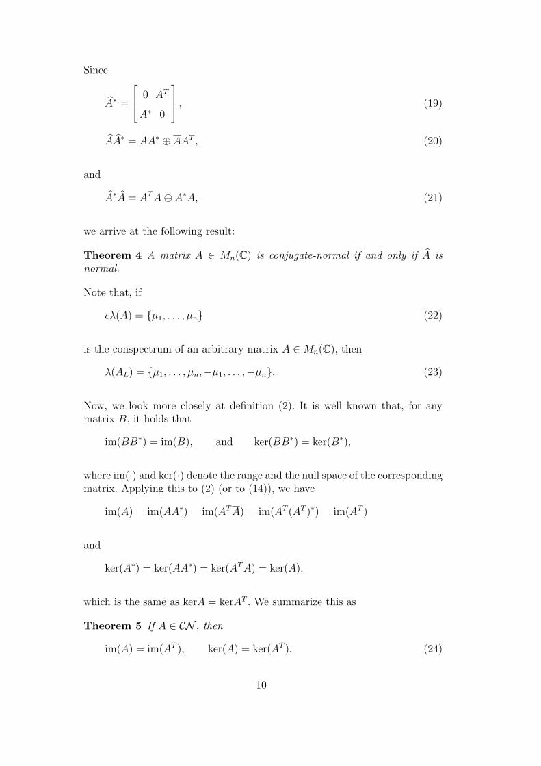
Since

A∗ =

0 AT

A∗ 0

, (19)

AA∗ = AA∗ ⊕ AAT , (20)

and

A∗A = AT A⊕ A∗A, (21)

we arrive at the following result:

Theorem 4 A matrix A ∈ Mn(C) is conjugate-normal if and only if A isnormal.

Note that, if

cλ(A) = {µ1, . . . , µn} (22)

is the conspectrum of an arbitrary matrix A ∈ Mn(C), then

λ(AL) = {µ1, . . . , µn,−µ1, . . . ,−µn}. (23)

Now, we look more closely at definition (2). It is well known that, for anymatrix B, it holds that

im(BB∗) = im(B), and ker(BB∗) = ker(B∗),

where im(·) and ker(·) denote the range and the null space of the correspondingmatrix. Applying this to (2) (or to (14)), we have

im(A) = im(AA∗) = im(AT A) = im(AT (AT )∗) = im(AT )

and

ker(A∗) = ker(AA∗) = ker(AT A) = ker(A),

which is the same as kerA = kerAT . We summarize this as

Theorem 5 If A ∈ CN , then

im(A) = im(AT ), ker(A) = ker(AT ). (24)

10

Below, we say more about the common properties of A and AT . For the mo-ment, we return to (2). Equating the entries on the left and the right, we findthat

{AA∗}ij =n∑

k=1

aikajk =n∑

k=1

akiakj = {A∗A}ij. (25)

The result obtained can be stated as follows.

Theorem 6 A matrix A ∈ Mn(C) is conjugate-normal if and only if relation(25) is fulfilled for each pair (i, j), 1 ≤ i, j ≤ n.

In other words, A ∈ CN n if and only if, for each pair (i, j), the scalar productof rows i and j is equal to the scalar product of columns i and j.

Corollary 1 If A ∈ CN n, then, for each i (1 ≤ i ≤ n), the 2-norm of row iis equal to the 2-norm of column i.

Corollary 2 Let Ai1,...,ik be the submatrix formed of rows i1, . . . , ik (i1 ≤ i2 ≤. . . ≤ ik) of a matrix A ∈ Mn(C). If A ∈ CN n, then

||Ai1,...,ik ||F = ||ATi1,...,ik

||F . (26)

Recall that a normal matrix A shares its invariant subspaces with the Hermi-tian adjoint A∗. We can prove an analogous fact for conjugate-normal matrices.

Theorem 7 Every coninvariant subspace of A ∈ CN n is also a coninvariantsubspace of AT .

Proof: Let Lk be a k-dimensional coninvariant subspace of A (1 ≤ k ≤n). Choose an orthonormal basis q1, . . . , qk in Lk, complement it to a basisq1, . . . , qk, qk+1, . . . , qn of the entire space Cn, and define

Q = [Q1︸︷︷︸k

Q2︸︷︷︸n−k

] = [q1 . . . qn],

B = QT AQ. (27)

Partition B in conformity with Q:

B =

B11 B12

B21 B22

.

11

Thus, B11 is a k × k block. Rewrite (27) as

AQ = QB. (28)

Then, the definition of a coninvariant subspace implies that

B21 = 0.

Since B ∈ CN , relation (26) yields

B12 = 0.

From (27), we derive

BT = QT AT Q

and

AT Q1 = Q1B11. (29)

Equality (29) means that Lk is a coninvariant subspace of AT . 2

Remark 2 The proof presented above gives more than just the assertion ofTheorem 7. Indeed, since B12 = 0, relation (28) yields

AQ2 = Q2B22.

Thus, L⊥ = span{qk+1, . . . , qn} is a coninvariant subspace of A.

We state this result as

Theorem 8 If L is a coninvariant subspace of a conjugate-normal matrix A,then L⊥ is also a coninvariant subspace of A.

Remark 3 Theorems 7 and 8 correspond to items 8 and 9 in the GJSW list.However, unlike the latter, they are not criteria, because the conditions inthese theorems do not imply that A is conjugate-normal.

Now, we examine the Youla form B of a conjugate-normal matrix A. Reasoningas in the proof of Theorem 7, we conclude that all the off-diagonal blocks inB are zero. Thus, the Youla form of A ∈ CN is a block diagonal matrix with1× 1 and 2× 2 diagonal blocks.

12

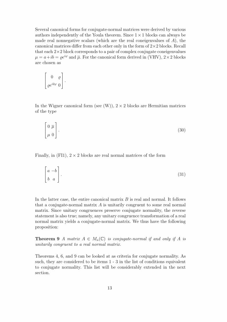
Several canonical forms for conjugate-normal matrices were derived by variousauthors independently of the Youla theorem. Since 1× 1 blocks can always bemade real nonnegative scalars (which are the real coneigenvalues of A), thecanonical matrices differ from each other only in the form of 2×2 blocks. Recallthat each 2×2 block corresponds to a pair of complex conjugate coneigenvaluesµ = a+ib = %eiϕ and µ. For the canonical form derived in (VHV), 2×2 blocksare chosen as

0 %

%ei2ϕ 0

.

In the Wigner canonical form (see (W)), 2× 2 blocks are Hermitian matricesof the type

0 µ

µ 0

. (30)

Finally, in (FI1), 2× 2 blocks are real normal matrices of the form

a −b

b a

. (31)

In the latter case, the entire canonical matrix B is real and normal. It followsthat a conjugate-normal matrix A is unitarily congruent to some real normalmatrix. Since unitary congruences preserve conjugate normality, the reversestatement is also true; namely, any unitary congruence transformation of a realnormal matrix yields a conjugate-normal matrix. We thus have the followingproposition:

Theorem 9 A matrix A ∈ Mn(C) is conjugate-normal if and only if A isunitarily congruent to a real normal matrix.

Theorems 4, 6, and 9 can be looked at as criteria for conjugate normality. Assuch, they are considered to be items 1 - 3 in the list of conditions equivalentto conjugate normality. This list will be considerably extended in the nextsection.

13

4 Conditions

In this section, we present a list of about forty conditions on a matrix A ∈Mn(C), each of which is equivalent to A being conjugate-normal. The firstcondition in this list is numbered 4 for the reasons explained at the end of theprevious section.

Some conditions involve an additional requirement of nonsingularity. In eachcase, such a restriction is indicated explicitly.

Most of the conditions in our list are counterparts of the appropriate conditionsin the GJSW or EI lists, and we indicate the locations of the latter in thoselists.

4. AT is conjugate-normal.5. A is conjugate-normal.6. A∗ is conjugate-normal.7. A−1 is conjugate-normal (for invertible A).

(Cf. condition 2 in the GJSW list.)8. A−1AT is unitary (for invertible A).

(Cf. condition 3 in the GJSW list.)9. A = A−T AA∗ (for invertible A). Thus, a matrix A ∈ CN is consimilar to

A, the transformation being specified by A∗.(Cf. condition 4 in the GJSW list.)

10. AA∗A = AT AA (or AAAT = AA∗A).(Cf. condition 74 in the EI list.)

11. AC = CA, where C = AA∗ − AT A.(Cf. condition 73 in the EI list. The matrix C is an analogue of theself-commutator [A, A∗] = AA∗ − A∗A.)

12. AB = BA implies that AT B = BA∗. In words, if A concommutes withsome matrix B, then AT concommutes with B as well.(Cf. condition 6 in the GJSW list.)

13. UT AU is conjugate-normal for any (or for some) unitary U .(Cf. condition 7 in the GJSW list.)

14. p(AA)A = Ap(AA) is conjugate-normal for any polynomial p with realcoefficients.(Cf. condition 1 in the GJSW list.)

15. There exists a polynomial p(z) with real coefficients such that

AT = p(AA)A = Ap(AA).

(Cf. condition 17 in the GJSW list.)16. The matrix A∗A− AA∗ is semidefinite.

(Cf. condition 20 in the GJSW list.)

14

The following eight conditions refer to the SSS decomposition of A (see (16).

17. SK = KS.(Cf. condition 21 in the GJSW list.)

18. AS = SA.(Cf. condition 22 in the GJSW list.)

19. AS + SA∗ = 2SS (or SA + A∗S = 2SS).(Cf. condition 23 in the GJSW list.)

20. AK = KA.(Cf. condition 24 in the GJSW list.)

21. AK −KA∗ = 2KK (or KA− A∗K = 2KK).(Cf. condition 25 in the GJSW list.)

22. S−1A+A∗S−1

= 2I (or AS−1 +S−1

A∗ = 2I), as long as S is nonsingular.(Cf. condition 26 in the GJSW list.)

23. K−1A− A∗K−1

= 2I (or AK−1 −K−1

A∗ = 2I), as long as K is nonsin-gular.(Cf. condition 27 in the GJSW list.)

24. SS −KK = AA∗.(Cf. condition 75 in the EI list.)

In the following conditions, cλ(A) = {µ, . . . , µn}, cλ(S) = {ζ1, . . . , ζn}, andcλ(K) = {iη1, . . . , iηn} (ηj ∈ R, 1 ≤ j ≤ n) are the conspectra of A, S, and K,respectively.

25. |µ1|2 + . . . + |µn|2 = ||A||2F .(Cf. condition 53 in the GJSW list.)

26. (Reµ1)2 + . . . + (Reµn)2 = ζ2

1 + . . . + ζ2n.

(Cf. condition 54 in the GJSW list.)27. (Imµ1)

2 + . . . + (Imµn)2 = η21 + . . . + η2

n.(Cf. condition 55 in the GJSW list.)

28. There exists a permutation δ ∈ Sn such that

cλ(A) = {ζj + iηδ(j)|j = 1, . . . , n}.

(Cf. condition 34 in the GJSW list.)29. Recλ(A) = {ζ1, . . . , ζn}.

(Cf. condition 35 in the GJSW list.)30. Imcλ(A) = {η1, . . . , ηn}.

(Cf. condition 36 in the GJSW list.)

The following conditions refer to symmetric-unitary polar decompositions (SUPDs)introduced in Section 2 (see (17)).

31. A and AT admit SUPDs A = SU and AT = SV with the same symmetricfactor S.(Cf. condition 71 in the EI list.)

15

32. There exists an SUPD of A such that AS = SA.(Cf. condition 39 in the GJSW list.)

33. There exists an SUPD of A such that USS = SSU.(Cf. condition 37 in the GJSW list.)

34. There exists an SUPD of A such that UA∗A = A∗AU.(Cf. condition 38 in the GJSW list.)

35. λ(AA∗) = {|µ1|2, . . . , |µn|2}.(Cf. condition 57 in the GJSW list.)

36. The singular values of A are |µ1|, . . . , |µn|.(Cf. condition 58 in the GJSW list.)

37. The coneigenvalues of the symmetric matrix S in any SUPD of A are|µ1|, . . . , |µn|.(Cf. condition 47 in the GJSW list.)

38. Suppose that the coneigenvalues µ1, . . . , µn of A are numbered so that|µ1| ≥ |µ2| ≥ . . . ≥ |µn|. Then,

s1 · · · sk = |µ1 · · ·µk|, 1 ≤ k ≤ n.

(Cf. condition 59 in the GJSW list.)39. A+ is conjugate normal.

(Cf. condition 60 in the GJSW list.)40. A+AT is a partial isometry.

(Cf. condition 61 in the GJSW list.)41. (Ax, Ay) = (AT x, AT y) for all x, y ∈ Cn.

(Cf. condition 62 in the GJSW list.)42. (Ax, Ax) = (AT x, AT x) for all x ∈ Cn.

(Cf. condition 63 in the GJSW list.)43. ||Ax||2 = ||AT x||2 for all x ∈ Cn.

(Cf. condition 64 in the GJSW list.)44. AT = UA for some unitary U .

(Cf. condition 65 in the GJSW list.)

For a matrix A with the conspectrum cλ(A) = {µ1, . . . , µn}, define the con-spectral radius as

cρ(A) = max1≤i≤n

|µi|.

45. ||Ck(A)||2 = cρ(Ck(A)), k = 1, 2, . . . , n− 1.(Cf. condition 88 in the EI list.)

5 Proofs and comments

Some of the conditions presented in Section 4 are obvious or can be verifiedby straightforward calculations. Several conditions are just restatements of the

16

others in the same list.

The main technical tool in proving most of the nontrivial conditions is The-orem 4. The following approach is used: for a given condition on A, find theappropriate condition on A in the GJSW or EI list. Since the latter conditionis equivalent to normality of A, the former is equivalent to A being conjugate-normal.

Let us illustrate this approach by several examples.

Proof of condition 12: Sufficiency is shown by setting B = A. Since AB =BA is trivially true for B = A, we must have AT A = AA∗, i.e., A is conjugate-normal. Now, let A ∈ CN , and let B concommute with A:

AB = BA. (32)

For

A =

0 A

A 0

and B =

0 B

B 0

,

we have

AB = AB ⊕ AB, BA = BA⊕BA.

In view of (32), A and B commute. Since A is normal, condition 6 in theGJSW list yields

A∗B = BA∗,

which is equivalent to

AT B = BA∗.

2

In this proof, the approach outlined above was used only in one direction. Letus consider a couple of examples where this approach is exploited in full.

Proof of condition 11: Formulas (18) - (21) show that the self-commutatorof A has the form

[A, A∗] = C ⊕ C,

17

where C = AA∗ −AT A. According to condition 73 in the EI list, A is normalif and only if A commutes with its self-commutator. Since

A

C 0

0 C

=

0 AC

AC 0

and

C 0

0 C

A =

0 CA

CA 0

,

the commutation condition amounts to the relation

AC = CA.

This relation is equivalent to A being conjugate-normal. 2

Proof of condition 40: It is easily verified that the Moore-Penrose inverseof A is given by

A+ =

0 A+

A+ 0

.

One possible way is to check four Moore-Penrose conditions defining the pseu-doinverse.

Condition 61 in the GJSW list says that A is normal if and only if A+A∗ is apartial isometry. Recall that a matrix B is called a partial isometry if B∗B isan orthoprojector. Since

A+A∗ =

A+AT 0

0 A+AT

,

we conclude that A+A∗ is a partial isometry if and only if A+AT is. Thus, thiscondition is equivalent to the conjugate normality of A. 2

Now that the approach involving A is clear, we discuss a few conditions forwhich this approach is inefficient.

Proof of condition 14: Sufficiency is easy: just set p(z) ≡ 1; then, p(AA)A =A is conjugate-normal. To prove necessity, consider a canonical form of theconjugate-normal matrix A. For definiteness, let B be the Wigner canonicalform of A. We should verify that p(BB)B is a matrix of the same blockdiagonal form as B. Each 1 × 1 block, i.e., a nonnegative scalar µ producesa scalar p(µ2)µ. The new scalars can be negative, but this is easily mended

18

by an additional congruence with a unitary diagonal transformation matrix.Each 2× 2 block in B (see (30)) transforms into

0 p(µ2)µ

p(µ2)µ 0

. (33)

Thus, p(BB)B is a canonical Wigner matrix, and p(BB)B (hence, p(AA)A)is conjugate-normal.

The assumption that p has real coefficients is important because, otherwise,the scalars p(µ2)µ and p(µ2)µ may not be conjugate. What is more important,they may have different moduli, which contradicts Corollary 1. 2

We are now going to prove condition 15, which corresponds to condition 17 inthe GJSW list. The latter reads ’there exists a polynomial p such that A∗ =p(A).’ It is not required that p have real coefficients. However, as shown byLaffey (L), one can always find a real polynomial p for the relation A∗ = p(A)with a normal A.

Proof of condition 15: Necessity. It is convenient to seek the desired poly-nomial p using the Wigner canonical form B of A. Thus, we want to have

BT = p(BB)B.

This yields

p(µ2)µ = µ (34)

for each real µ, which is automatically fulfilled if µ = 0 and is a nontrivialcondition for each positive coneigenvalue µ.

For 2× 2 blocks, we require that

0 p(µ2)µ

p(µ2)µ 0

=

0 µ

µ 0

(see (30)), which reduces to two scalar relations

p(µ2)µ = µ (35)

19

and

p(µ2)µ = µ. (36)

Now, relations (34) written for all distinct positive µ and relations (35)-(36)written for all distinct complex conjugate pairs (µ, µ) constitute a Vander-monde-like system of linear equations with respect to the coefficients of thepolynomial p. Thus, the system is solvable. Its solution is unique if we restrictthe degree of p by m− 1, where m is the number of equations.

The special feature of our system is that, along with an equation with com-plex coefficients, it contains the one with the conjugate coefficients. Since thesolution is unique, it must be real.

Sufficiency. From AT = p(AA)A, we derive

AA∗ = AAT = Ap(AA)A = Ap(AA)A

(note that the last equality uses the fact that p has real coefficients) and

A∗A = AT A = p(AA)AA = Ap(AA)A.

Thus, A ⊂ CN . 2

Proof of condition 31: Sufficiency. Let A = SU and AT = SV , where Uand V are unitary. Then,

AA∗ = (SU)(U∗S) = SS

and

A∗A = AT A = (SV )(V ∗S) = SS.

Hence, A is conjugate-normal.

Necessity. Perform a unitary congruence that transforms the conjugate-normalmatrix A into a real normal matrix B. Observe that, in the polar decomposi-tion of B, the symmetric factor P and the orthogonal factor W commute:

B = PW = WP.

It follows that

BT = PW T .

20

Performing the reverse congruence transformation, we obtain SUPDs for Aand AT having the same symmetric factor S. 2

Note that conditions 32 – 34 can be proved following the same pattern. Thedetails can be found in (FI2).

Proof of condition 44: Sufficiency. If AT = UA for a unitary U , then

(AT x, AT y) = (UAx, UAy) = (Ax, Ay) ∀x, y ∈ Cn.

By condition 41, A ∈ CN .

Necessity. First, bring A and AT by a unitary congruence transformation totheir Wigner canonical forms B and BT :

B = QAQT , BT = QAT QT . (37)

Then for each 2× 2 block 0 %e−iϕ

%eiϕ 0

in B (see (30)) form the diagonal matrix

ei2ϕ 0

0 e−i2ϕ

. (38)

The direct sum of matrices of type (38) complemented by an identity matrix(which corresponds to the 1× 1 blocks in B) yields a diagonal unitary matrixD such that

BT = DB.

Finally, we reverse transformation (37):

AT = Q∗BT Q = Q∗DBQ = (Q∗DQ)(Q∗BQ) = UA.

Thus, U = Q∗DQ is the desired unitary matrix. 2

21

Proof of condition 45: The coneigenvalues of Ck(A) squared are the ordi-nary eigenvalues of

Ck(A)Ck(A) = Ck(A)Ck(A) = Ck(AA). (39)

If µ1, . . . , µn (|µ1| ≥ |µ2| ≥ . . . ≥ |µn|) are the coneigenvalues of A, then theeigenvalues of matrix (39) are all the possible k-products

µ2i1µ2

i2· · ·µ2

ik

with 1 ≤ i1 < i2 < . . . < ik ≤ n (see (MM, p. 24)). It follows that

cρ(Ck(A)) = |µ1| · · · |µk|.

On the other hand,

||Ck(A)||2 = s1 · · · sk.

Thus, condition 45 is just a disguised form of condition 38. 2

6 Concluding remarks

The discussion presented above is not exhausting. Several interesting prop-erties of conjugate-normal matrices were left outside the scope of this paper.Here, we briefly mention one of these properties.

It is well known that normal matrices are perfectly conditioned with respect tothe problem of calculating their eigenvalues. A similar fact can be establishedfor the coneigenvalues of a conjugate-normal matrix. More on this can befound in (GI).

It was shown in Remark 1 that the normality of AL and AR does not implythat A is conjugate-normal. Matrices defined by the requirement that AL (orAR) be normal were introduced in (HLV) and were called congruence-normalmatrices there. This is an interesting matrix class standing farther from normalmatrices than conjugate-normal matrices. We intend to discuss this class in aseparate paper.

22

References

[EI] L. Elsner and Kh.D. Ikramov. Normal matrices: an update. LinearAlgebra Appl., 285:291–303, 1998.

[FI1] H. Faßbender and Kh.D. Ikramov. Some observations on theYoula form and conjugate-normal matrices. Linear Algebra Appl.,422:29–38, 2007.

[FI2] H. Faßbender and Kh.D. Ikramov. A note on an unusual type ofpolar decomposition. submitted 2007.

[GI] A. George and Kh.D. Ikramov. Conditionality and expected errorfor two methods of computing the coneigenvalues of a complexmatrix. Comput. Math. Math. Physics, 35:1403–1408, 1995.

[GJSW] R. Grone, C.R. Johnson, E.M. Sa and H. Wolkowicz. Normalmatrices. Linear Algebra Appl., 87:213–225, 1987.

[HLV] F. Herbut, P. Loncke and M. Vujicic. Canonical form for matricesunder unitary congruence transformations. II. Congruence-normalmatrices. SIAM J. Appl. Math., 26:794–805, 1974.

[HJ1] R.A. Horn and C.R. Johnson. Matrix Analysis. Cambridge,University Press, Cambridge, 1990.

[HJ2] R.A. Horn and C.R. Johnson. Topics in Matrix Analysis. Cam-bridge, University Press, Cambridge, 1991.

[L] T.J. Laffey. A normality criterion for an algebra of matrices.Linear Algebra Appl., 25:169–174, 1979.

[MM] M. Marcus and H. Minc. A survey of matrix theory and matrixinequalities. Dover, 1992.

[VHV] M. Vujicic, F. Herbut and G. Vujicic. Canonical form for matricesunder unitary congruence transformations. I. Conjugate-normalmatrices. SIAM J. Appl. Math., 23:225–238, 1972.

[W] E.P. Wigner Normal form of antiunitary operators. J. Math.Phys., 1:409–413, 1960.

[Y] D.C. Youla. A normal form for a matrix under the unitary con-gruence group. Canad. J. Math., 13:694–704, 1961.

23