Conical Pendulum Part 3: Further Analysis with Calculated ...

European J of Physics Education Volume 9 Issue 2 1309-7202 Dean

14

Conical Pendulum Part 3:

Further Analysis with Calculated Results of the

Period, Forces, Apex Angle, Pendulum Speed and

Rotational Angular Momentum

Kevin Dean

Physics Department,

Khalifa University of Science and Technology,

SAN Campus, PO Box 127788, Abu Dhabi,

United Arab Emirates

[email protected]

(Received: 25. 11. 2018, Accepted: 01. 12. 2018)

Abstract The conical pendulum provides a rich source of theoretical and computational analysis and the present work

presents a seamless continuation of the previous publication. The tension force FT and centripetal force FC are explored further in linearization analyses and the appropriate slopes are explained. A similar analysis is applied to the period as a visual confirmation of the expected linearity and the slope is explained. The apex angle is

considered as a function of both the conical pendulum period and angular speed. An analysis is presented of the conditions required for the constancy of the length of the adjacent side of the triangle defining the conical pendulum, which gives rise to an apparently counter-intuitive result and this is explained in detail. The speed

of the rotating conical pendulum mass is calculated as a function of the radius and also as a function of the apex angle. The rotational speed is then used in order to calculate the rotational angular momentum. In order to

maintain continuity of calculations from the previous work, the length range of the conical pendulum was

maintained to be 0.435 m L 2.130 m, the local acceleration due to gravity g = 9.789 ms-2

and with a mass

m = 0.1111 kg. This required the same limits for the string tension of approximately mg FT 12 N, the

calculations therefore covered an apex angular range from zero (string hanging vertically down) up to 85. Keywords: Conical pendulum, theoretical analysis, tension force, centripetal force, period, angular frequency, rotational speed, angular momentum, high-precision, computational analysis.

INTRODUCTION

The conical pendulum has been extensively studied both experimentally and theoretically, with

varying degrees of precision, accuracy, mathematical rigor, approximation and correctness. As

an example, for the situation where the orbital radius R is considered to be much smaller than the

length L of the conical pendulum string (R L), the orbital rotational period T was equated to the oscillation period of a standard simple pendulum (Richards, 1956). This approximation is

surprisingly good, for example with L = 1.000 m, R = 0.030 m and g = 9.789 ms-2

(the value used

throughout this paper), the simple pendulum equation gives an oscillation period of 2.008 s (to 4

significant figures). The correct equation (derived in Dean & Mathew, 2017 and also Dean,

2017) gives a conical pendulum period of 2.00777 s 2.008 s (again to 4 significant figures).

An electric motor-driven conical pendulum has been used to determine a value for the


15

acceleration due to gravity and was claimed to be repeatedly capable of yielding results with a

quoted precision of approximately 1% (Klostergaard, 1976).

When coupled to a computer-controlled data-acquisition system, (Moses and Adolphi, 1998),

experimental results can be obtained by students, which are very reproducible and have a short

acquisition time, thereby allowing time for further student exploration. An experiment has been

reported (Dupré and Janssen, 1999), which is suitable for undergraduate students to perform and

has a stated accuracy of approximately 0.1%, using a rotating rod and an appropriate data

measurement system. The conical pendulum has been used as an explanatory example of the

dynamics of circular motion (Czudková and Musilová, 2000), in order to highlight and answer

specific test questions relating to the mathematical and conceptual understanding of circular

motion. The fundamental physics laws of conservation of angular momentum and mechanical

energy have been very successfully demonstrated by using a variable length conical pendulum

and an experimentally unsophisticated apparatus, with a simple timing system (Bambill, Benoto

and Garda, 2004). The experiment was stated to produce results that were good enough to

illustrate the conservation laws and the experimental setup was a simple one to use.

An imaginative and successful conical pendulum experiment has been reported, based on the

circular motion of a tethered model aero-plane (Mazza, Metcalf, Cinson and Lynch, 2007). The

experiment utilized a digital video camcorder and video pointer as well as the usual mechanical

apparatus. The overall assessment of the success of this imaginative experiment, suggested that

the results obtained were satisfactory, with an accuracy stated to be close to 2%. An electric

motor-driven, small length (0.199 m) conical pendulum was investigated in detail with specific

reference to obtaining a value for the acceleration due to gravity. The average published value of

g was 9.97 ms – 2

which is in reasonable agreement with the accepted value.

Classical mechanics is applied to the detailed analysis of the conical pendulum (this being one

example among several that were considered). Dimensional analysis is used to facilitate the

derivation of elliptical precession and a suitable set of equations is derived (Deakin, 2012). A

complex three-dimensional analysis of the Foucault pendulum, with reference to the conical

pendulum, performed in a rotating frame of reference (Barenboim and Oteo, 2013) provides a

series of trajectory equations for the motional path. The theory of dynamic interactions of some

circular systems is investigated in detail (Lacunza, 2015), leading to the motion trajectory for the

mass of a conical pendulum, by using D’ Alembert’s principle for classical mechanics.

Regarding the present paper, in order to maintain complete continuity with previous work,

this extension of the conical pendulum analysis is based on the same figure (shown below) that

was used in the first two papers that form part of this multi-part series, (Dean & Mathew, 2017

and Dean, 2017). It is noted that the conical pendulum mass (which is considered to be a point-

mass) is maintained at m = 0.1111 kg, all theoretical calculations were performed using the local

value of the acceleration due to gravity g = 9.789 ms-2

(Ali, M.Y.et al., 2014). The conical

pendulum string was considered to be essentially of negligible mass (compared to the conical

pendulum mass) and also physically inextensible.


16

Figure 1. Conical Pendulum Schematic

To identify the lines that have been calculated and then plotted on the Excel charts, the reader

is referred to the Appendices that contain the chart legend, (except for Chart 3).

THEORETICAL RESULTS AND ANALYSIS

The analysis that follows in this section continues directly from the immediately preceding

publication relating to the conical pendulum (Dean, 2017). Inspection of the equation below

enables a reasonably good approximation to be obtained in the limit of (R L), such that the conical pendulum orbital period can be easily calculated from the oscillating period equation of a

simple pendulum. It is noted that this approximation is surprisingly good (up to 4 significant

figures), when (R 0.03L) i.e. for when R is close to 3% of the conical pendulum length L.

g

L

L

R

g

L

g

RL

g

LT

2122

cos2

2

222

The tension force FT has been shown (Dean, 2017) to be given by the equation below, which

can be readily plotted as a straight-line Chart, such that the slope has a value of (mg) providing

an experimental value for the local acceleration due to gravity.

2

cos

Lm

gmFT

(1)

(2)


17

Chart 1. FT against 1/cos ()

The centripetal force FC given by the equation below, can also be plotted as a straight line as

shown in Chart 2, where the slope again has the value of (mg), thus providing an alternative

experimental value for the gravitational acceleration.

2tan RmgmFC

Chart 2. FC against tan ()

(3)


18

Since the tension force FT and the centripetal force FC are seen to be trigonometric functions

of the apex angle (although different functions), it was considered as being visually useful to

calculate and plot the respective first derivatives (dFT /d and dFC / d ) of both forces:

coscostan

coscos

sin

cos

2

2

TCC

CTT

Fgm

d

FdgmF

Fgm

d

FdgmF

Close inspection of the above two derivative functions shows that for very small apex angles

that are asymptotically approaching zero degrees ( 0), the denominators of both derivative equations are approximately one. Therefore, (by considering the numerators of both derivative

equations), the calculated first derivative of the tension force (dFT /d ) asymptotically goes to

zero, whilst the calculated first derivative of the centripetal force (dFC /d ) asymptotically goes to the numerical value of (mg), as shown in Chart 3. It is also observed that both first derivative

functions progressively appear to merge together when 80 and this is especially noticeable

beyond 85. As an example, when = 85 the first derivative of the tension force (dFT /d ) has a value (stated to 4 significant figures and in the appropriate SI units) of 142.6, whereas the first

derivative of the centripetal force (dFC /d ) has a value of 143.2, which differ by only 0.4%.

Chart 3. Derivatives of FT and FC against Apex angle

(4)


19

The conical pendulum period has been studied in detail and an equation derived (Dean, 2017)

that shows the square of the period T 2 to be directly proportional to the square of the period for a

simple pendulum [TSP ] 2 multiplied by the cosine of the apex angle.

cos][coscos

2 22

SPSP TTTg

LT

This provides a straight line having a value for the slope equal to exactly 1 (Chart 4).

Chart 4. T 2 against (TSP) 2 cos ()

It is of interest to consider the dependence of the Apex angle as a function of the orbital

period of the conical pendulum squared T 2, by making a simple algebraic re-arrangement:

L

Tg

g

LT

g

LT

2

21

2

2

4cos

cos

4

cos2

This functional equation is plotted in Chart 5. The fact that all of the curves originate from a

calculated (although physically unrealizable) value of = 90 can be explained, by considering that the minimum possible value for the conical pendulum period must coincide with the

pendulum rotating at the highest possible orbital speed, which occurs in the mathematical limit

of 90. It is important to note that the curves calculated for this chart are representative of

the behavior of the arc-cosine function and do not take the practical physical limitations into

account. The variation of the two forces (tension and centripetal) can be inferred, by considering

the first two calculated charts.

(5)

(6)


20

As the period progressively increases, then the apex angle must correspondingly

progressively decrease, which is clearly shown in Chart 5.

Chart 5. Apex angle against T 2

An alternative (entirely equivalent) representation can be used where the angular frequency

squared 2 is taken as the horizontal axis parametric variable and plotted in Chart 6.

Chart 6. Apex angle against 2


21

The equation describing this parametric dependence is shown (7)

2

1

2

21 cos

4cos

L

g

L

Tg

When the angular frequency approaches the limit of a minimum vale min for each of the

calculated lines for the different length conical pendulums, then the apex angle correspondingly

decreases to the asymptotic limit of = 0 (being equivalent to the situation for an oscillating simple pendulum). As the angular frequency progressively increases, the apex angle must also

increase asymptotically towards the limiting value of 90 (this mathematical limit cannot be

achieved physically, since it would require the angular frequency to approach infinity).

A further straightforward re-arrangement of an earlier equation enables an alternative method

of obtaining an experimental value for the gravitational acceleration. The required equation is

obtained in the following way:

2

2

4cos

cos2

TgL

g

LT

Chart 7. L cos () against T 2

The experimental data consists of the conical pendulum period and the measured vertical

distance between the conical pendulum support point and the horizontal plane of rotation. As

shown in Chart 7, the calculated slope of the graphical straight line can provide an experimental

value the gravitational acceleration.

(7)

(8)


22

In order to extend the analysis further, the orbital speed was derived as a function of the

orbital radius, according to the self-explanatory analysis outlined in the equations below:

4/12222

22

2

2cos

2

RL

RgR

RL

g

T

Rv

g

RL

g

LT

Although the final equation (9) for the orbital speed appears to be somewhat complicated, it

is in fact very readily calculated and contains only a single parametric variable. For R = 0

(corresponding to the situation where the conical pendulum hangs vertically downwards), the

orbital speed must also be zero for all values of the conical pendulum length L. As the orbital

radius progressively increases, so that R L, the denominator asymptotically tends to zero, so

that the orbital speed v and this is clearly seen in Chart 8.

Chart 8. Orbital speed v against Radius R

The orbital speed can easily be re-expressed as an uncomplicated function of the apex angle,

which can then be readily calculated. Starting with equation (9) for the orbital speed and then

making appropriate trigonometric substitutions for the orbital radius R in the numerator and also

for the function of L 2

and R 2

that appears in the denominator, yields a simple equation that can

be used to calculate the functional dependence of the orbital speed v.

(9)


23

cos

sin

cos

sin4/122

LgL

Lg

RL

Rgv

Consideration of the numerator of this equation indicates that when the apex angle is zero,

the chart lines must all start at the origin of coordinates, so = 0 is equivalent to R = 0 for the

preceding chart (Chart 8), where the conical pendulum is observed to be vertical. As the apex

angle progressively increases 90 the denominator of the equation approaches zero, and so therefore the orbital speed increases and asymptotically tends to infinity (this mathematical limit

being physically unattainable). Chart 9 shows this for the angular range 0 < 90.

Chart 9. Orbital speed v against Apex angle

When the conical pendulum mass rotates in circular motion it possesses angular momentum,

that will be represented in scalar terms by the lower-case letter l = Rmv in the usual format. This

has been calculated as a function of the orbital radius as follows in the self-explanatory analysis

shown below:

4/122

2

4/122 RL

RgmvmRl

RL

Rgv

The dependence of the magnitude of the angular momentum as a function of the orbital

radius is shown in Chart 10. The fact that l varies according to the square of the orbital radius is

very clearly shown. The numerator of the equation indicates that for R = 0, all lines must start at

the coordinate origin (just as for the speed against orbital radius). The visual appearance of the

(10)

(11)


24

orbital speed curves and the angular momentum curves is very similar. However, the angular

momentum curves increase more rapidly and become asymptotic more far abruptly.

Chart 10. Angular Momentum against Radius R

In a similar way to the dependence of the orbital speed, the angular momentum was also

considered as function of the apex angle as shown in the derivation below:

cos

sin

cos

sinsin

cos

sin

22/3Lgml

LgmLvmRl

Lgv

It can be observed from Chart 11, which illustrates the functional shape of the angular

momentum curves, starting at the origin of coordinates (due to = 0 in the equation numerator)

and progressively increasing steeply until becoming asymptotic towards infinity at high angles,

which is to be expected from the square-root cosine term present in the denominator.

(12)


25

It can be observed from the series of Chart 11 curves, that the angular momentum steepens

progressively and very rapidly becomes near-vertical for apex angles 85. This is again a

direct consequence of the root cosine term that is present in the denominator.

Chart 11. Angular Momentum against Apex angle

From the mathematical representation of the physical parameters that have been investigated,

it becomes apparent that the conical pendulum period, forces, speeds and momentum equations

might possibly be combined and investigated further. One interesting example analysis is

presented below, which deals with the constancy of the length of the adjacent side of the

schematic triangular construction used for analyzing the conical pendulum (refer to Chart 7).

ANALYSIS (Length of adjacent side = constant)

By considering the conical pendulum period equation T, a straightforward analysis leads to an

interesting (and virtually counter-intuitive) result, which is explained in detail below:

cos2cos

22

22

Lgg

L

g

RLT

For any particular value of the conical pendulum period T, the following can be readily

obtained for two different conical pendulum lengths L1 and L

2 that have the same period:

2211

2

22211 coscos4

cos2

cos2

LLTg

Lg

Lg

T


26

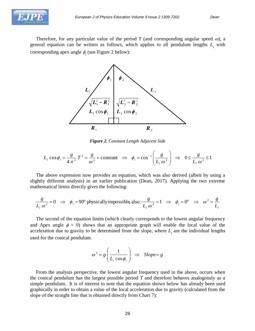
Therefore, for any particular value of the period T (and corresponding angular speed ), a

general equation can be written as follows, which applies to all pendulum lengths Li with

corresponding apex angle i (see Figure 2 below):

Figure 2. Constant Length Adjacent Side

10cosconstant4

cos22

1

2

2

2

ii

iiiL

g

L

ggT

gL

The above expression now provides an equation, which was also derived (albeit by using a

slightly different analysis) in an earlier publication (Dean, 2017). Applying the two extreme

mathematical limits directly gives the following:

i

i

i

i

i L

g

L

g

L

g 2

2201:also ,impossible physically900

The second of the equation limits (which clearly corresponds to the lowest angular frequency

and Apex angle = 0) shows that an appropriate graph will enable the local value of the

acceleration due to gravity to be determined from the slope, where Li are the individual lengths

used for the conical pendulum.

gSlopeL

gii

cos

12

From the analysis perspective, the lowest angular frequency used in the above, occurs when

the conical pendulum has the largest possible period T and therefore behaves analogously as a

simple pendulum. It is of interest to note that the equation shown below has already been used

graphically in order to obtain a value of the local acceleration due to gravity (calculated from the

slope of the straight line that is obtained directly from Chart 7):


27

2

2

2 44cos

gSlopeT

gL ii

DISCUSSION OF RESULTS AND CONCLUSIONS

The analysis and associated charts that are presented in this paper develop from the previously

published paper that discussed mathematically some of the fundamental physics involved in the

rotational motion of a conical pendulum. The tension and centripetal force are both shown to be

linear, as trigonometric functions of the apex angle (one being a reciprocal cosine and the other a

tangent). It is shown that for both of the associated charts, the respective straight-line slopes are

equal to the constant (mg), from which a value for the local acceleration due to gravity can be

readily obtained. The square of the conical pendulum period (derived in the previous paper) was

demonstrated to be linear with respect to the product of the square of the period of a simple

pendulum and the cosine of the apex angle. The functional dependence of the apex angle was

shown using two equivalent (but subtly different) time parameters as the horizontal axis, namely,

the square of the period and the square of the angular frequency. Both charts were explained in

detail, especially the point of origin of curves and any asymptotic behavior. A linear chart is

included, which shows that when the distance between the point of support and the rotational

plane is plotted as a function of the square of the period, the slope of the resulting straight line

provides another method to determine the acceleration due to gravity. The orbital speed and also

the corresponding rotational angular momentum were analyzed as functions of the orbital radius

and apex angle and appropriate charts were plotted and explained in detail.

APPENDIX

Chart legend for theory lines (except Chart 3)

Figure 3. Chart Legend


28

REFERENCES

Ali, M. Y., Watts, A. B., & Farid, A. (2014). Gravity anomalies of the United Arab Emirates:

Implications for basement structures and infra-Cambrian salt distribution. GeoArabia, 19(1),

85-112.

Bambill, H. C. R., Benito, M. R., & Garda, G. R. (2004). Investigation of conservation laws

using a conical pendulum. European journal of physics, 25(1), 31-35.

Barenboim, G., & Oteo, J. A. (2013). One pendulum to run them all. European Journal of

Physics, 34(4), 1049.

Czudková, L., & Musilová, J. (2000). The pendulum: A stumbling block of secondary school

mechanics. Physics Education, 35(6), 428.

Deakin, M. A. (2013). The ellipsing pendulum. International Journal of Mathematical Education

in Science and Technology, 44(5), 745-752.

Dean, K., Matthew, J. (2017). Conical Pendulum – Linearization Analysis . European Journal of

Physics Education, 8(1), 38-52.

Dean, K. J. (2017). Conical Pendulum: Part 2 A Detailed Theoretical and Computational

Analysis of the Period, Tension and Centripetal Forces. European Journal of Physics

Education, 8(1), 11-30.

Dupré, A. and Janssen, P. (1999). An accurate determination of the acceleration of gravity g in the

undergraduate laboratory. American Journal of Physics, 68, 704-711.

Klostergaard, H. (1976). Determination of gravitational acceleration g using a uniform circular

motion. American Journal of Physics, 44(1), 68-69.

Lacunza, J. C. (2015). The Pendulum of Dynamic Interactions. Journal of Applied Mathematics

and Physics, 3(09), 1186.

Mazza, A. P., Metcalf, W. E., Cinson, A. D., & Lynch, J. J. (2007). The conical pendulum: the

tethered aero-plane. Physics education, 42 (1), 62.

Moses, T. and Adolphi, N.L., (1998). A new twist for the conical pendulum. The Physics

Teacher, 36 (6), 372-373.

Richards, J.A., (1956). Conical pendulum. American Journal of Physics, 24 (9), 632.

Tongaonkar, S. S., & Khadse, V. R. (2011). Experiment with Conical Pendulum. European

Journal of Physics Education, 2(1), 1-4.

Conical Pendulum Part 3: Further Analysis with Calculated ...

Documents

Transcript of Conical Pendulum Part 3: Further Analysis with Calculated ...