Confounded coefficients: Accurately comparing logit and probit coefficients across

groups

Glenn Hoetker

College of Business Administration University of Illinois at Urbana-Champaign

350 Wohlers Hall 1206 S. Sixth Street

Champaign, IL 61820 Tel: 217-355-4891 Fax: 217-244-7969

E-mail: ghoetker@uiuc.edu

ABSTRACT

The logit and probit models are critical parts of the management researcher’s analytical

arsenal. We often want to know if a covariate has the same effect for different groups, e.g.,

foreign and domestic firms. Unfortunately, many attempts to compare the effect of covariates

across groups make the unwarranted assumption that each group has the same residual variation.

If this is not the case, comparisons of coefficients can reveal differences where none exist and

conceal differences that do exist. This article explains the statistical and substantive implications

of this assumption, introduces approaches to comparing coefficients that avoid making it, and

uses simulations to explore the practical significance of the assumption and the power of

approaches introduced to avoid it. As a practical example, I show that an apparent dramatic new

insight into the technology strategy of Japanese computer manufacturers is actually just a

manifestation of this problem. I close with implications for the practice of research.

Keywords: Logit, probit, discrete choice

INTRODUCTION

The logit and probit models have become critical parts of the management researcher’s

analytical arsenal. In strategy, marketing, and organizational economics, they are the primary

tool for analyzing the make-or-buy decision (Anderson and Schmittlein 1984; Masten 1984;

Shelanski and Klein 1995). International business researchers use them to analyze firms’ choice

of entry mode into a foreign country (Barkema and Vermeulen 1998; Chen and Hennart 2002).

Researchers have also applied them to study consumer purchasing behavior given the presence

of a store brand (Chintagunta, Bonfrer, and Song 2002), the likelihood of a person remaining in

the teaching profession (Stinebrickner 2001), and incumbent firms’ decision to enter an

emerging industrial subfield or not (Mitchell 1989).

Often it is of interest to know if a covariate has the same effect for different groups. For

example, Kim, Han and Srivastava (2002) asked whether Windows and Macintosh users gave

equal consideration to network externalities in their decision to upgrade their hardware. Long,

Allison, and McGinnis (1992) studied whether the number of articles published affected the

likelihood of promotion for male and female faculty equally.

Unfortunately, attempts to compare the effect of logit or probit coefficients across groups

require an assumption that is often false. Logit and probit coefficients are scaled by the unknown

variance of their residual variation. Naïvely comparing coefficients as one would in linear

models assumes that residual variation is the same across groups, though in many cases it may

not be. Differences in coefficients across groups may merely reflect the difference in residual

variation across groups, rather than real differences in the impact of covariates across groups.

Recently, Allison (1999a) drew attention to the pitfalls of assuming equal residual variation

across groups in the sociological literature, but most management research does not reflect

awareness of the issue. Yet the consequences of violating this assumption are severe. As Allison

expresses it, “Differences in the estimated coefficients tell us nothing about the differences in the

underlying impact of x on the two groups” (1999a:190). Worse yet, they may appear informative.

1

They can reveal differences where none exist, conceal differences that do exist, and even indicate

differences in the reverse direction of the actual situation.

This paper has four goals. First, it seeks to make researchers aware of the dangers of

comparing coefficients across groups while naively assuming their residual variation is the same.

Second, it equips researchers with a set of analytical techniques that avoid this assumption. Third,

it uses simulations to explore the practical significance of the ignoring the assumption of equal

residual variation and the power of alternative analytical techniques. To my knowledge, this is

the first time this has been done. Lastly, it brings together the first three points to suggest

implications for the practice of research.

The article proceeds as follows. After briefly reviewing the logit and probit models, I explain

the statistical implications of comparing coefficients across groups without accounting for

possible differences in the groups’ residual variation. I then use a simulated dataset to

demonstrate the substantive implications of doing so: even small differences in the groups’

residual variation can lead to extremely misleading results. Next, I introduce several approaches

for comparing coefficients that avoid the assumption of equal residual variation and explore their

power with simulated data. I demonstrate the importance and practical application of these

methods using actual data on the technology procurement strategies of U.S. and Japanese

notebook computer manufacturers. The paper concludes with a discussion of implications for the

practice of research using logit and probit.

IMPLICATIONS OF ASSUMPING EQUAL RESIDUAL VARATION ACROSS GROUPS

Statistical implication of the assumption

Since standard econometric texts (e.g., Greene 2000) and more specialized works (Allison

1999b; Long 1997; Maddala 1983; Train 1986) cover the logit and probit models, this section

will review the logit model only briefly, focusing on the elements relevant to this paper.

Suppose we are modeling which of two alternatives occurs, e.g., whether a firm makes or

buys a component. Without loss of generality, we assign a value of 0 to the dependent variable yi

for cases in which one alternative occurs and set yi equal to 1 for cases in which the other

2

alternative occurs. We assume that y equals 1 only if an unobserved, continuous variable y* is

greater than an unobserved threshold, τ. That is,

≤

>=

τ

τ*

*

if 0

if 1

i

ii y

yy

(1)

Further, we assume that y* is linearly related to the observed independent variables:

iiy ε+= αxi*

(2)

where xi is a vector of observed covariates and εi is a random disturbance independent of the

observed covariates. As in the linear model, the disturbance reflects the impact of differences

across cases in variables the researcher does not observe—residual variation.

Since y* is a latent variable, we cannot estimate its variance, mean, or the threshold, τ. In the

logit model, we assume ε has a logistic distribution and variance 1. In the probit case, we assume

ε is normally distributed with a variance of π2/3. Again, these arbitrary values are assigned

because they simplify calculations, however they cannot be confirmed by the data. τ and E(ε|x)

are typically assumed to be 0 as an identifying assumption.

These assumptions lead to the familiar logit modeli

βxi=

− i

i

pp

1log (3)

The β coefficients we obtain from estimating equation (3) are related to the α coefficients in

equation (2) as follows.

σαβ = (4)

where σ is the standard deviation of the residual variation, ε. This relationship is the heart of

the problem in comparing coefficients across groups. Since the true value of σ is unidentifiable,

we cannot recover α, the true effect of a covariate. When we arbitrarily set σ equal to 1, we also

arbitrarily set the scale of β. Accordingly, if σ varies between groups, the logit coefficient β will

also vary, even if the true effect of the covariate,α, is the same between groups.

3

Substantive implications of the assumption

In many contexts, it is reasonable to assume that residual variation differs across groups. For

example, institutional pressures may lead Japanese firms to be more similar in their strategy than

U.S. firms (Lincoln 2001). In labor mobility studies, there is evidence that women have more

heterogeneous career paths than men (Long and Fox 1995).

There is a heavy burden of proof on any author claiming that residual variation is the same

across groups, because the failure of this assumption can have serious consequences. To

demonstrate these consequences, consider the following hypothetical model, which uses a

simulated dataset. We wish to model the dichotomous variable y as a result of two independent

variables, x1 and x2. We are particularly interested in knowing whether the effect of x2 on the

likelihood of y=1 differs across two groups, which I unimaginatively label “Group 0” and

“Group 1”. I generated the data according to equation (5). ii

≤

>=

++=

0 if 0

0 if 1

2

*

*

21*

i

ii

iii

y

yy

xxy ε

x1, x2 ~ N(µ=0,σ=4) εgroup 0~N(µ=0, σ=2) εgroup 1~N(µ=0, σ=4)

(5)

Note that the actual impacts of x1 and x2 are the same for both groups. Only the residual

variation differs across groups. For simplicity, I assume the two groups are the same size and that

group membership is exogenous, e.g., gender or firm’s home country.iii

There are two common approaches to comparing coefficients across groups: comparing the

coefficients that result from estimating separate models for each group or estimating a single

model that interacts a variable for group membership with variables of interest. Table 1 reports

the results of the first approach. I estimated the following equation twice, once for each group.

221101log xx

pp

i

i βββ ++=

−

(6)

Naively comparing the results, we see an apparent difference in the impact of x2. It appears to

have almost twice as strong an effect (1.835/.922) for Group 0 as for Group 1. In a linear model,

4

we would use the Wald chi-squared statistic to determine if the difference in the estimated

coefficients is statistically significant. Assuming the coefficients for each group have

independent sampling distributions, the statistic is

( )( )[ ] ( )[ ]22

221

2

202

12

.... GG

GG

errstderrstd ββ

ββ

+

−, (7)

which has one degree of freedom. Applying it to the coefficients for x2 yields a statistic of 31.12,

which is highly significant (p<.001). We would thus conclude that the effect of x2 differs across

groups. This conclusion is, of course, false, since by construction the only difference between the

two groups is the standard deviation of their residual variation. Unfortunately, in a real world

application, we would not know the residual variation in each group and could not tell if

differences in coefficients indicate differences in actual effect.

Table 2 extends this simulation to show how severe the problem can become with even small

differences in the residual variation. I again generated data using Equation (5), but let the

standard deviation of Group 1’s residual variation range from 1 to 2 in increments of 0.2. I

generated 20 datasets of 1000 observations each for the five different standard deviations. The

table shows the results of estimating Equation (6) on each dataset. The first column shows that

the estimated value of β2 decreases quickly as the standard deviation increases, even though the

true value of the coefficient, α2, is exactly the same in each dataset. The next column uses

Equation (7) to test for the equality of β2 between Group1 and Group 0 (for which the standard

deviation was held at 1.0). When Group 1’s standard deviation was 1.2, the coefficients were

incorrectly found to differ at the five percent level of significance in 6 out of 20 cases. Larger

differences in the residual variation led to more false results, as one would expect. For example,

when the standard deviation of Group 1’s residual variation was 1.6, the coefficients were found

to differ in 17 out of 20 cases. This clearly illustrates the hazards of comparing coefficients

across groups if their residual variation might differ.

The second approach to comparing the effect of a covariate across groups is to estimate a

single regression for all observations (Aiken and West 1991; Pindyck and Rubinfeld 1991). A

5

dummy variable is set to one for one type of observation, e.g., Group1, and interacted with the

relevant covariates. Considering a linear model with only one variable, x, and letting the dummy

variable, G, be set to 1 for Group 1 firms, the equation would be of the form

iiii xGxy εβββ +++= )(210 (8)

An estimate of β2 significantly different from 0 indicates that the impact of x varies between

Group 0 and Group 1. The sign of β2 indicates whether the impact of x is diminished or increased

for Group 1.

As indicated by the presence of a single error term, εi, this approach assumes that the residual

variation for Group 0 and Group 1 is the same (Darnell 1994:111; Pindyck and Rubinfeld

1991:107). We can test this assumption in the linear model (Quandt 1960), but as discussed

above, we cannot test it in a logit model, because the standard deviation of the residual variation

cannot be identified and has been arbitrarily set to 1 (Long 1997:47; Maddala 1983:23).

Therefore, the single equation approach is inappropriate unless there are strong theoretical

reasons to believe that the residual variation is the same in both groups.

A variation of the above simulation demonstrates how misleading this sort of comparison can

be. I generated 20 simulated datasets of 1000 observations each, 500 each from Group 0 and

Group 1, according to the following equation.

=

≤

>=

+++=

1 groupfor 10 groupfor 0

0 if 0

0 if 1

)(5.2

*

*

221*

i

i

ii

iiiii

G

y

yy

xGxxy ε

x1, x2 ~ N(µ=0, σ=4) εgroup 1~N(µ=0, σ=1) εgroup 1~N(µ=0, σ=3)

(9)

I then estimated the equation

( )23221101log xGxx

pp

ii

i ββββ +++=

−

(10)

6

on each dataset. A significant coefficient for β3 would indicate that x2’s impact on the

dependent variable differs across groups. Even though x2’s effect is 25% greater for Group 1 by

design, estimating Equation (10) fails to find this difference. Figure 1 shows the point estimate

and 95% confidence intervals for β3 in each of the 20 simulated datasets. The 95% confidence

interval included the true value of the coefficient, 0.5, in only four datasets: 4, 7, 8 and 13. Of

those, the estimated coefficient was significant in only one dataset, number 4. Disturbingly, the

only other statistically significant estimate, dataset 9, is a highly erroneous -0.42, indicating a

diminished impact of x2, rather than the true increased impact.

This unfortunate outcome is not surprising. The likely outcome of using an interaction term

in a single equation despite differences in variance between the groups is that the slope

coefficients will be found not to differ, even if they actually do (Gujarati 1988: 527). However,

dataset 9 shows that it is also possible to find an effect contrary to reality. Clearly, the single

equation with interaction term strategy is no better than estimating each group separately.

In fact, it is even less informative. In the single equation model, it is impossible to determine

if the coefficient has a significant effect within a group. In contrast, the separate equations

reported in Table 1 show that β2 was statistically significant for both Group 0 and Group 1.

To summarize, we cannot compare coefficients across groups in a logit or probit model as we

would in a linear regression. Doing so, either by regressing each group separately and comparing

coefficients or by using an interaction term in a single equation, can lead to erroneous

conclusions. Insignificant differences can appear significant and significant differences can

appear insignificant. Clearly, we need a way to identify a difference in residual variation across

groups and to carry out accurate comparisons even in its presence.

IDENTIFYING AND ADJUSTING FOR UNEQUAL RESIDUAL VARIATION

Allison’s method

Allison (1999a) developed a set of related tests to determine if (a) the residual variation of

two groups differs significantly, (b) if there is evidence that the true effect of at least one

covariate differs significantly across groups, and (c) if the true effect of a specific covariate

7

differs across groups. I will only briefly sketch the underpinnings to this method, focusing on

demonstrating its power and relative ease of application. This section introduces Allison’s

method and uses simulations to test its power. The next section uses a practical example to

demonstrate its application in detail.

At the heart of the approach is rewriting the underlying model as a single equation that

allows the residual variation to vary across groups. Under the assumption that all coefficients are

equal across the groups, we can write the model as

1,1

11 groupfor 10 groupfor 01j

10*

−>+

=

=

+++= ∑>

δδ

σ

σβββ

ii

i

iiijjii

G

G

exGy

(11)

Arbitrarily setting σ equal to 1 for group 0, δ>0 implies that the residual variation is smaller

for Group 1 than Group 0. If δ<0, the residual variation is larger for Group 1 than Group 0. The

standard deviation of the residual variations differs by 100δ percent.

Combining this with Equation (3) leads to

( )ij

ijjii

i GxGp

pδβββ +

++=

− ∑

>

11

log1

10 , (12)

which can be estimated using code supplied by Allison.iv

The first test proceeds under the null hypothesis that the true values of the coefficients are the

same across groups, but that the residual variation differs. That is, it tests that the α terms are the

same, but that σ varies across groups. The test proceeds by estimating equation (12) and

examining . We can determine if is significantly different from zero by a Wald chi-square

test (the squared ratio of the estimate to its standard error). Alternatively, we can construct a log-

likelihood ratio test by taking twice the positive difference between the log-likelihood for this

model and the log-likelihood for an ordinary logit equation (equivalent to assuming δ=1). If is

not significant, the test provides no evidence that the residual variation differs between groups.

In this case, Allison suggests continuing with conventional methods for comparing coefficients.

δ̂ δ̂

δ̂

8

If, on the other hand, is significantly different from zero, it is evidence that the residual

variation differs across groups. The residual variation differs by 100 percent between groups,

with a positive value indicating that Group 1’s residual variation is greater than Group 0’s.

δ̂

δ̂

If we find unequal residual variation, the next step is to test the null hypotheses that the true

coefficients (the α terms) are the same across groups versus the alternative hypotheses that at

least one of them varies. Since the model estimated immediate above constrains the α terms to be

equal across groups, we need to compare it to an unconstrained model that allows the α

coefficients to vary across groups. We do so with a likelihood ratio test. We can obtain the log-

likelihood for the unconstrained model either by estimating an ordinary logit model that interacts

every covariate with the group membership dummy, G, or by adding together the log-likelihoods

obtained by estimating a separate logit model for each group.

I return to the earlier simulation to explore the power of this method. To improve on

conventional practice, it should meet three criteria. First, it should reveal when residual variation

differs significantly between groups. Second, it should detect when apparent differences in

coefficients across groups are merely the impact of differences in residual variation. Third, it

should allow us to detect true differences of coefficients across groups.

I first test the method’s performance when the underlying coefficients, the α’s in Equation

(3), are the same and only the residual variation varies across groups. I generated datasets of

1000 observations (500 of Group 0, 500 of Group 1) according the following equation:

≤

>=

++=

0 if 0

0 if 1

2

*

*

21*

i

ii

iii

y

yy

xxy ε

x1, x2 ~ N(µ=0, σ=4) εgroup 0~N(µ=0, σ=1)

εgroup 1~N(µ=0, σ=1,1.2, 1.4, 1.6, 1.8)

(13)

I varied the standard deviation of Group 1’s residual variation from 1 to 1.8. At each level, I

generated 20 datasets.

9

I then tested for differences in residual variation by estimating equation (12) on each dataset.

The first two columns of Table 3 report the results. The method does moderately well in meeting

the first criteria, detecting differences in residual variation between groups. When the standard

deviation of Group 1’s residual variation is 1.8 versus 1.0 for Group 0, is significantly

different from zero in 18 out of 20 cases (17 out of 20 using a likelihood ratio test). That is, the

method accurately indicated a difference in residual variation in the overwhelming majority of

cases. When the difference is more moderate, a standard deviation of 1.4 versus 1.0, both the

Wald and log-likelihood ratio tests indicate a significant difference in residual variation in about

half of the simulated data sets. Importantly, the test yields few false positives. When the residual

variation was equal across groups, the method indicated so in 17 out of 20 cases (Wald test).

That is, it falsely indicated that residual variation differed across groups in only 3 of the 20 cases.

δ̂

The third column shows the results of testing the null hypothesis that the true coefficients are

all equal across groups versus the alternative that at least one differs. Allison’s test correctly

indicated that there is no actual difference in the coefficients in 19 out of 20 cases at each level

of Group 1’s residual variation. That is, it incorrectly rejected the null hypothesis of no

difference in only 1 of 20 cases. To emphasize the improvement over conventional tests,

compare the results to Table 2. There, the conventional test incorrectly indicated that x2’s effect

differed across groups in 6 out of 20 cases when Group 1’s residual variation had a standard

deviation of 1.2, and in 14 out of 20 cases when the standard deviation was 1.4. Clearly, the test

meets the second criteria for improving on current practice.

I next test the method’s ability to detect true differences in the value of a coefficient across

groups, the third criteria. I again generated datasets of 500 Group 0 and 500 Group 1

observations, this time using Equation (14). It fixes the standard deviation of Group 1’s residual

variation slightly higher than that of Group 0 and varies γ, the additional impact of x2 for Group 1,

from 0 to 1 in 0.2 increments. Since the coefficient for x2 is 2 for Group 0, this range represents

an equal to fifty-percent greater effect for Group 1. For each value of γ, I generated 20 datasets.

10

( )

=

≤

>=

+++=

1 groupfor 10 groupfor 0

0 if 0

0 if 1

2

*

*

21*

i

i

ii

iiii

G

y

yy

xGxy εγ

x1, x2 ~ N(µ=0, σ=4) εgroup 0~N(µ=0, σ=1) εgroup 1~N(µ=0, σ=1.4)

γ =0, 0.2, 0.4, 0.6, 0.8, 1.0

(14)

The first two columns of Table 4 report on the method’s ability to detect differences in the

residual variation across groups. When x2 has the same effect in both groups, the method

accurately reports that the residual variation differs in just over half the sample datasets.

Unfortunately, the method becomes less able to detect the difference in residual variation across

groups as x2’s additional impact on Group 1 increases. When x2 has a 20% greater impact on

Group 1 (γ=.4), the method identifies the difference in residual variation in only 6 of 20 cases.

Since we know from Table 2 that this degree of difference in residual variation can lead to false

conclusions about differences in coefficients, this result raises concerns.

The third column of the table reports on the method’s ability to detect real difference in

coefficients across groups. When x2 has a 10% greater impact on Group 1 (γ=.2), the method

reports the difference in only 4 of 20 cases. However, when the difference is 20%, (γ= .4), it

detects the difference in 15 of 20 cases. It continues to improve as the difference increases, as

one would expect.

It is also theoretically possible to test the null hypothesis that all of the underlying

coefficients are the same against the alternative hypothesis that a specific coefficient, e.g., x2,

differs across groups. However, the test assumes that all of the coefficients not being tested are

the same across groups. We cannot test this assumption without engaging in circular logic. To

test whether the coefficients for x2 differ, we must assume that the coefficients for x1 are the

same. However, we cannot test that assumption without assuming that the coefficients for x2 are

11

the same. Given this limitation, the scope for applying this test is limited and I will not test its

power. I do, however, demonstrate its use in the practical example below.

In general, simulation results are somewhat reassuring about our ability to detect and resolve

the confounding effect of different residual variation across groups. However, even when the

difference in the standard deviation of the residual variation was forty percent, Allison’s method

failed to indicate this difference in almost half of the cases. Still, by identifying the difference in

even half the cases, it greatly improves on naïve comparison of coefficients and should be

routinely applied.v However, it is not a panacea. Therefore, I will present two other approaches.

Differences in the relative effect of covariates

Given the limitations of the method above, particularly its inability to show whether a

specific coefficient differs across groups, we may want to consider an approach that renders any

difference in residual variation irrelevant. Suppose we could frame our interest not as whether

the absolute effect of x2 differed across groups, but rather as whether the impact of x2 relative to

x1 differs across groups. To answer this question, we compare the ratio β2/β1 (Train 1998:237). If

this ratio were 2 for Group 0 and 3 for Group 1 it would mean that a “unit” of x2 has twice the

effect of a unit of x1 for Group 0 and thrice the effect of a unit of x1 for Group 1. Relative to x1, x2

has a stronger effect on Group 1.

When this sort of comparison is sensible and theoretically interesting, the nature of ratios

provides us a powerful benefit. Since β is the underlying coefficient, α, scaled by the standard

deviation of the residual variation, σ, we find that

1

2

1

2

1

2

1

2

αα

ασ

σα

σασ

α

ββ

=

== . (15)

By taking a ratio, we have removed the impact of residual variation and are left with a ratio

of the underlying effects of x2 and x1. We can compare this ratio across groups, since it is no

longer confounded by differences in residual variation.

12

The statistical significance of the difference in the ratios across groups can be computed with

a Wald chi-squared test (Greene 2000).vi Unfortunately, even large differences in ratios may not

be statistically significant, especially if one or more terms are estimated with poor precision. To

demonstrate this, I generated data according to Equation 14 above and then compared the ratio of

β2 to β1 resulting from estimating

221101log xx

pp

i

i βββ ++=

−

(16)

separately for each group.

Table 5 shows the results given sample sizes of 100 and 1000. When the true coefficient of x2

is 2.4 for Group 1 versus 2.0 for Group 0, the difference in the ratio β2/β1 across groups is

statistically significant in 15 of 20 simulated datasets of 1000 observations. With only 100

observations, however, we detect the difference in only 8 of 20 datasets. The difference becomes

more extreme when the true value of x2 rises to 2.8 for Group 1. With 1000 observations, we

detect the difference in β2/β1 across groups in every case. With only 100 observations, however,

we detect the difference in only twelve cases. Clearly, we need more precise estimates and thus

more observations to apply this technique than we need to compare individual coefficients.

Abandon direct comparisons

Given these challenges, a researcher may wish to simply abandon direct comparisons of

coefficients across groups. Even in this case, we can often make some analytical progress.

If we model the two groups separately, the coefficients and standard errors are consistent

within each group. The pattern of coefficient significance between the two models may provide

some information. If β1 were positive and highly significant for Group 0 and far from significant

for Group 1, it suggests that x1 has a stronger effect on Group 0 than on Group 1. While not a

formal test, the fact that the effect of x1 is indistinguishable from 0 for Group 1 strongly suggests

that x1 has a larger effect for Group 0. In essence, “not zero” is a larger effect than “zero”.

Obviously, this suggestion is stronger if the samples are of roughly the same size and the model

appears well specified. The suggestion is also stronger if the p-values do not straddle a particular

13

significance level. For example, it would be foolish to draw strong implications from one p-value

being .09 and the other .11, even though the latter does fall outside of the conventional 10% level

of significance.

Of course, if a coefficient is (in)significant for both groups, this approach does not provide

insight into relative effects. However, the researcher can at least report that, for example, x1 has a

significantly positive impact for both groups.

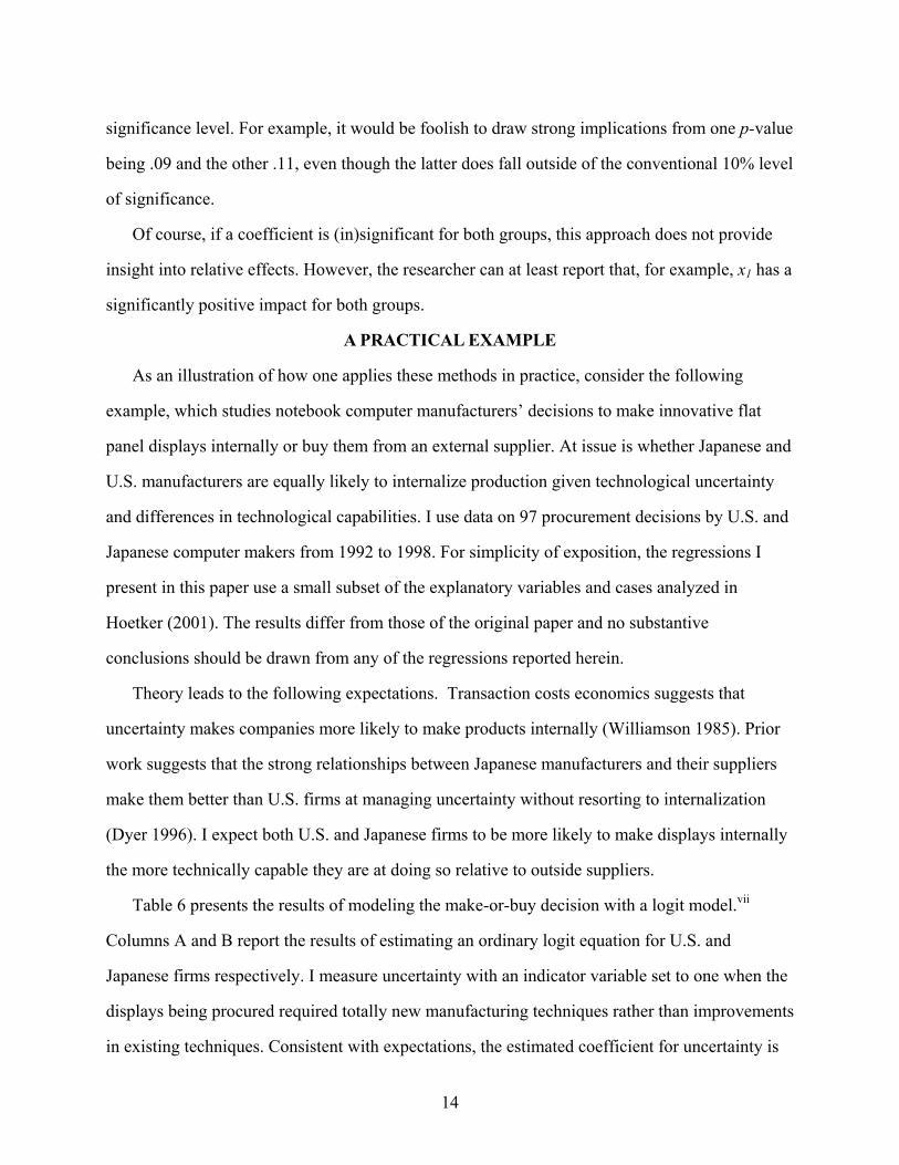
A PRACTICAL EXAMPLE

As an illustration of how one applies these methods in practice, consider the following

example, which studies notebook computer manufacturers’ decisions to make innovative flat

panel displays internally or buy them from an external supplier. At issue is whether Japanese and

U.S. manufacturers are equally likely to internalize production given technological uncertainty

and differences in technological capabilities. I use data on 97 procurement decisions by U.S. and

Japanese computer makers from 1992 to 1998. For simplicity of exposition, the regressions I

present in this paper use a small subset of the explanatory variables and cases analyzed in

Hoetker (2001). The results differ from those of the original paper and no substantive

conclusions should be drawn from any of the regressions reported herein.

Theory leads to the following expectations. Transaction costs economics suggests that

uncertainty makes companies more likely to make products internally (Williamson 1985). Prior

work suggests that the strong relationships between Japanese manufacturers and their suppliers

make them better than U.S. firms at managing uncertainty without resorting to internalization

(Dyer 1996). I expect both U.S. and Japanese firms to be more likely to make displays internally

the more technically capable they are at doing so relative to outside suppliers.

Table 6 presents the results of modeling the make-or-buy decision with a logit model.vii

Columns A and B report the results of estimating an ordinary logit equation for U.S. and

Japanese firms respectively. I measure uncertainty with an indicator variable set to one when the

displays being procured required totally new manufacturing techniques rather than improvements

in existing techniques. Consistent with expectations, the estimated coefficient for uncertainty is

14

positive for both U.S. and Japanese manufacturers, indicating that internalization is more likely

given higher uncertainty. However, it is only statistically significant for U.S. firms.

More striking is the difference in the estimated coefficients for relative technical strength,

which I measured as the ratio between the manufacturer’s display-related patents and the

maximum number of display-related patents held by any external supplier. We would expect a

positive effect, as firms are more likely to internalize production when they are technologically

stronger than available external suppliers. I find this result for U.S. firms, but not for Japanese

firms. Moreover, the estimated coefficient is much higher for U.S. firms (3.04) than Japanese

firms (.025). In the linear case, I would test the significance of the difference with a Wald chi-

squared test (Equation 7). Doing so in this case suggests that the difference is statistically

significant (chi-squared=7.11, p-value=0.007).

If true, this has profound implications. It means Japanese firms will tolerate a much larger

gap between their external supplier’s capabilities and their own before they internalize

production. While I might explain this result as evidence of Japanese firms’ strong commitment

to the outsourcing system, it suggests that Japanese firms use a very different calculus than do

U.S. firms when balancing the advantages of internal technological strength against the

bureaucratic costs of internalization. It also raises questions about why Japanese firms invest

almost as heavily in research and development as do U.S. firms (Ministry of Economy, Trade

and Industry (Japan) 2001), if they strongly prefer to outsource despite being technically strong

relative to external suppliers.

Before racing to declare my finding a breakthrough, I need to consider the possibility that

differences in residual variation have confounded my comparisons. I apply Allison’s method to

explore this possibility.

I first test if residual variation differs significantly between groups. Estimating equation (12)

yields an estimate of -0.87 for δ (Column D). This indicates that the standard deviation of the

residual variation is 87 percent lower for Japanese firms than U.S. firms. I compute the

significance of the δ coefficient with a Wald chi-squared test (the squared ratio of the estimate to

15

its standard error), which yields (.87/.17)2 =26.2 with one degree of freedom (p<.01).

Alternatively, I can use a standard log-likelihood ratio test to compare the model to an ordinary

logit model estimated on all firms, which constrains σ to be the same for both groups (Column

C). Calculating twice the positive difference between the log-likelihoods yields 2*(33.32-

28.43)=9.79. This has 2 degrees of freedom, since there are two more estimated coefficients in

the unconstrained equation than the constrained equation. Again, the result is significant (p=.07).

There is clear evidence that the residual variation differs across Japanese and U.S. companies.

Accordingly, I next test the null hypothesis that all of the underlying coefficients are the same for

U.S. and Japanese firms versus the alternative hypotheses that at least one coefficient varies. I do

this by comparing the log-likelihood of the most recent model (Column D), which constrains the

coefficients to be equal across groups while allowing the residual variation to differ, to a model

that interacts each variable with the Japanese-firm dummy. Conveniently, the log-likelihood of

the latter is equal to the sum of the log-likelihoods of the separate group regressions, Columns A

and B. The relevant calculation, 2*(28.43-(13.37+13.96)), yields a value of 2.2. This has one

degree of freedom, since the constrained model has five parameters and the unconstrained

models have six total parameters. This implies a p-value of .14. I am unable to reject the null

hypothesis that all of the underlying coefficients are the same across groups.

Therefore, I must conclude that the differences between the Japanese and U.S. coefficients

were merely the result of differences in the residual variation between the two groups of firms.

My dramatic original finding was a consequence of coefficients being confounded with residual

variation. Had I not tested for this possibility, I would have been misled about the behavior of

Japanese firms.

Purely for purposes of illustration, I next test whether the effect of relative technical strength

differs for Japanese companies. As noted above, this requires assuming that the effect of

uncertainty is the same across groups, an assumption I would not make in practice. Furthermore,

I have already found no evidence that any coefficient differs across groups. I proceed by

expanding the model in Column D to include an interaction between technical strength and

16

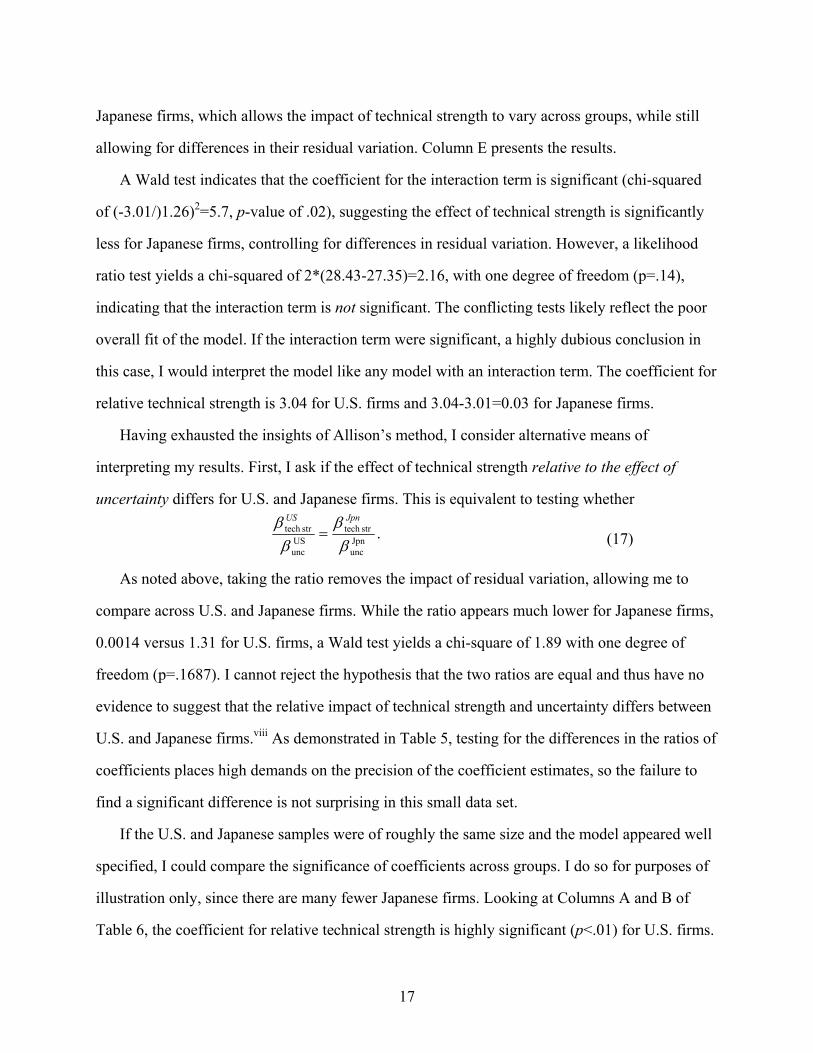
Japanese firms, which allows the impact of technical strength to vary across groups, while still

allowing for differences in their residual variation. Column E presents the results.

A Wald test indicates that the coefficient for the interaction term is significant (chi-squared

of (-3.01/)1.26)2=5.7, p-value of .02), suggesting the effect of technical strength is significantly

less for Japanese firms, controlling for differences in residual variation. However, a likelihood

ratio test yields a chi-squared of 2*(28.43-27.35)=2.16, with one degree of freedom (p=.14),

indicating that the interaction term is not significant. The conflicting tests likely reflect the poor

overall fit of the model. If the interaction term were significant, a highly dubious conclusion in

this case, I would interpret the model like any model with an interaction term. The coefficient for

relative technical strength is 3.04 for U.S. firms and 3.04-3.01=0.03 for Japanese firms.

Having exhausted the insights of Allison’s method, I consider alternative means of

interpreting my results. First, I ask if the effect of technical strength relative to the effect of

uncertainty differs for U.S. and Japanese firms. This is equivalent to testing whether

Jpnunc

strtech USunc

strtech

ββ

ββ JpnUS

= . (17)

As noted above, taking the ratio removes the impact of residual variation, allowing me to

compare across U.S. and Japanese firms. While the ratio appears much lower for Japanese firms,

0.0014 versus 1.31 for U.S. firms, a Wald test yields a chi-square of 1.89 with one degree of

freedom (p=.1687). I cannot reject the hypothesis that the two ratios are equal and thus have no

evidence to suggest that the relative impact of technical strength and uncertainty differs between

U.S. and Japanese firms.viii As demonstrated in Table 5, testing for the differences in the ratios of

coefficients places high demands on the precision of the coefficient estimates, so the failure to

find a significant difference is not surprising in this small data set.

If the U.S. and Japanese samples were of roughly the same size and the model appeared well

specified, I could compare the significance of coefficients across groups. I do so for purposes of

illustration only, since there are many fewer Japanese firms. Looking at Columns A and B of

Table 6, the coefficient for relative technical strength is highly significant (p<.01) for U.S. firms.

17

In contrast, for Japanese firms, it is far from significant ( p=.96). While not a formal test, a “more

than zero” effect for U.S. firms is likely larger than an “indistinguishable from zero” effect for

Japanese firms, suggesting that technical strength has a larger effect for U.S. firms.

Uncertainty is also significant for U.S. firms (p=.07), but not for Japanese firms (p=.13).

Even in the ideal case, however, I would not place much stock in this difference, given how close

the p-value for Japanese firms was to conventional significance levels.

In summary, this analysis initially appeared to offer a dramatic new insight into Japanese

technology strategy. It appeared that Japanese firms tolerate a much larger gap between their

external supplier’s capabilities and their own before they internalize production. However, more

appropriate analysis suggests that Japanese and U.S. firms probably do not differ in the impact of

technological strength on the probability of internalization. The apparent difference is actually

nothing more than the confounding of coefficients and differences in residual variation between

Japanese and U.S. firms.

IMPLICATIONS FOR RESEARCH

The implications for research using the logit or probit model are profound. Conclusions

drawn from comparing coefficients across groups while ignoring the possibility of coefficients

being confounded with residual variation are meaningless. The simulations in this paper have

shown that in the presence of even fairly small differences in residual variation, naïve

comparisons of coefficients can indicate differences where none exist, hide differences that do

exist, and even show differences in the opposite direction of what actually exists. As the U.S.–

Japan example shows, what appear to be dramatic new insights are likely to have no real basis.

This has implications for both gathering data and carrying out statistical testing.

Gathering as complete a set of covariates as possible is more important when using logit or

probit than when using linear regression. In the linear case, omitted variables are only significant

if they are correlated with included variables. However, in the logit or probit case, any variable

that helps explain the outcome variable is useful and should be gathered. The more variation we

18

control for, the less residual variation there is and the less it can vary across groups. We also

need a sizable sample to apply the ratio of coefficients technique.

Econometric theory and simulation results suggest that tests interacting coefficients with a

dummy variable for group membership in a single equation are particularly misleading. Forcing

observations from both groups to have the same residual variation yields coefficients that tell us

nothing about how a covariate’s impact varies across groups. Moreover, it yields no information

about the effect of the covariate on each group.

Estimating separate equations for each group at least offers the advantage of accurate

estimation within each group. However, before attempting to compare coefficients, researchers

must test for differences in residual variation. This will require a change in current practice, but

the test is simple to run in any statistical package.

If a difference in residual variation is found, the researcher has several options. Allison’s test

for determining if at least one coefficient differs between groups is powerful and makes few

assumptions. It will lead to more conservative results and may reveal that apparent differences

are not actually significant. If it reveals differences, the researcher can then test that a specific

coefficient differs. However, this test has a stringent assumption: the other coefficients must be

equal across the groups. Since it is not possible to test this, the researcher must judge the

probability of this assumption holding on theoretical grounds.

If it is theoretically relevant to compare the relative effects of two covariates across groups,

the researcher can compare the ratio of coefficients across groups. This has the advantage of

making no assumptions about the residual variation across groups. Offsetting this advantage are

two facts. First, an answer in terms of relative effects may not satisfy the theoretical question at

hand. Second, even large differences between ratios may not be statistically significant,

particularly if one or more terms are poorly estimated. This makes it more difficult, perhaps

artificially so, to identify cross-group differences.

Alternatively, the researcher can abandon attempts to compare the effects of covariates

directly. By modeling each group separately, the researcher can at least draw inferences about

19

the significance of coefficients within each group. Careful examination of the pattern of

coefficient significance across groups may suggest that a covariate has an impact in one group

and no impact in another.

In most cases, a combination of approaches will provide the most insight. For example,

suppose x2 is highly significant for Group 0, but far from significant for Group 1. Furthermore,

Allison’s test indicates that at least one covariate differs across groups. Lastly, the ratio β2/β1 if

significantly more for Group 0 than for Group 1. By several measures, we can argue that x2 plays

a more important role for Group 0 than Group 1.

Comparing coefficients across groups in logit or probit models requires that the researcher

apply careful judgment using his or her understanding of both statistical issues and the

underlying phenomenon. Ultimately, however, researchers may simply not be able to conduct

some of the comparisons they are accustomed to doing in the linear setting. While this is

frustrating, no results are surely superior to spurious results.

ACKNOWLEDGEMENTS

I gratefully acknowledge the helpful comments of Paul Allison, Tim Liao, and Steve Michael.

All errors remain my own.

20

Table 1: Apparent coefficient differences in simulated data

Group 0 Group 1X1 0.958*** 0.482***

(0.086) (0.041) X2 1.835*** 0.922***

(0.153) (0.062) Intercept 0.146 0.027

(0.147) (0.106)

Log likelihood -153.32 -287.68

N 1,000 1,000

Standard errors in parentheses*** p<0.01;** p<0.05; * p<0.1; two-tailed tests

Data generated according to the equation:

≤

>=

++=

0 if 0

0 if 1

2

*

*

21*

i

ii

iii

y

yy

xxy ε

x1, x2 ~ N(µ=0, σ=4)

εgroup 0~N(µ=0, σ=2)

εgroup 1~N(µ=0, σ=4)

21

Table 2: Differences in residual variation drive apparent differences in estimated coefficients

Standard deviation of

residual variation for

Group 1

Mean value of

estimated β2 for

Group 1

Number of times β2 was falsely found to differ across groups

(20 simulations, p=.05)

1.0 3.77 2 1.2 3.08 6 1.4 2.66 14 1.6 2.41 17 1.8 2.01 20 2.0 1.85 20

Data generated according to the equation:

≤

>=

++=

0 if 0

0 if 1

2

*

*

21*

i

ii

iii

y

yy

xxy ε

x1, x2 ~ N(µ=0, σ=4)

εgroup 0~N(µ=0, σ=1)

εgroup 1~N(µ=0, σ=1, 1.2, 1.4, 1.6, 1.8, 2.0)

22

Table 3: Allison's method accurately detects differences in residual variation and false differences in coefficients

Standard deviation of Group 1’s

residual variation

Does the standard deviation of the residual variation differ across

groups?

Number of positive tests out of 20 datasets (p=.05)

Do any of the coefficients differ across groups?

Number of positive tests out of 20 datasets (p=.05)

Wald chi-square testLog-

likelihood test Log-likelihood test 1.0 3 2 1 1.2 6 3 1 1.4 11 12 1 1.6 14 14 1 1.8 18 17 1

Data reflect estimating

221101log xx

pp

i

i βββ ++=

−

separately for Group 0 and Group 1 on data generated by

≤

>=

++=

0 if 0

0 if 1

2

*

*

21*

i

ii

iii

y

yy

xxy ε

x1, x2 ~ N(µ=0,σ=4)

εgroup 0~N(µ=0, σ=1)

εgroup 1~N(µ=0, σ=1.4)

23

Table 4: Allison's method also accurately detects true differences in coefficients

Additional impact of x2 on Group 1

Does the standard deviation of the residual variation differ across

groups?

Number of positive tests out of 20 datasets (p=.05)

Do any of the coefficients differ across groups?

Number of positive tests out of 20 datasets (p=.05)

Wald chi-square testLog-

likelihood test Log-likelihood test 0.0 11 12 1 0.2 8 7 4 0.4 6 5 15 0.6 2 3 18 0.8 2 3 20 1.0 2 2 20

Data reflect estimating

( )23221101log xGxx

pp

ii

i ββββ +++=

−

separately for Group 0 and Group 1 on data generated by ( )

=

≤

>=

+++=

1 groupfor 10 groupfor 0

0 if 0

0 if 1

2

*

*

21*

i

i

ii

iiii

G

y

yy

xGxy εγ

x1, x2 ~ N(µ=0, σ=4)

εgroup 0~N(µ=0, σ=1)

εgroup 1~N(µ=0, σ=1.4) γ ranges from 0 to 1

24

Table 5: Comparing the ratios of coefficients requires precise estimates of each coefficient

Additional impact of x2 on Group 1

Does the ratio 12 ββ differ across groups?

Number of positive

tests out of 20 datasets (p=.05)

N=100

Does the ratio 12 ββ differ across groups?

Number of positive

tests out of 20 datasets (p=.05)

N=1,000

0.0 5 1 0.2 8 3 0.4 8 15 0.6 10 18 0.8 12 20 1.0 14 20

Results reflect estimating

221101log xx

pp

i

i βββ ++=

−

separately for Group 0 and Group 1 on data generated by

( )

=

≤

>=

+++=

1 groupfor 10 groupfor 0

0 if 0

0 if 1

2

*

*

21*

i

i

ii

iiii

G

y

yy

xGxy εγ

x1, x2 ~ N(µ=0, σ=4),

εgroup 0~N(µ=0, σ=1)

εgroup 1~N(µ=0, σ=1.4) γ ranges from 0 to 1

25

Table 6: Probability of internalization for U.S. and Japanese manufacturers Ordinary logit Allison’s method (A) (B) (C) (D) (E)

U.S.

Firms Japanese

firms All firms Relative technical strength 3.041*** 0.025 1.56*** 2.99** 3.04**

(1.047) (0.555) .354 (1.04) (1.05) Uncertainty 2.306* 1.788 1.616** 2.5** 2.31*

(1.277) (1.193) .702 (1.26) (1.26) Intercept -7.04** -0.057 4.024*** -7.0 -7.04**

(2.15) (1.369) .760 (2.1) (2.16) Japanese firm 2.66 6.97**

(5.20) (2.77) δ (Japanese firm) -.87*** -.22

(.17) (.67) J. firm * rel. tech. strength -3.01**

(1.26) Log likelihood -13.37 -13.96 -33.32 -28.43 -27.35

N 74 23 97 97 97 Standard errors in parentheses. *** p<0.01;** p<0.05; * p<0.1; two-tailed tests

26

Figure 1: Estimates using an interaction term are highly misleading

True value of beta 3

Zero

-1-.7

5-.5

-.25

0.2

5.5

.75

1

Poi

nt e

stim

ate

and

95%

con

fiden

ce in

terv

alof

bet

a 3

1 2 3 4 5 6 7 8 9 10 11 12 13 14 15 16 17 18 19 20Simulated data set

Results reflect estimating

( )23221101log xGxx

pp

ii

i ββββ +++=

−

on data generated by

=

≤

>=

+++=

1 groupfor 10 groupfor 0

0 if 0

0 if 1

)(5.2

*

*

221*

i

i

ii

iiiii

G

y

yy

xGxxy ε

x1, x2 ~ N(µ=0, σ=4) εgroup 0~N(µ=0, σ=1) εgroup 1~N(µ=0, σ=3)

27

References

Aiken, L.S., and S.G. West. 1991. Multiple regression: testing and interpreting interactions.

Thousand Islands, CA: Sage Publications.

Allison, P.D. 1999a. Comparing logit and probit coefficients across groups. SMR/Sociological

Methods & Research 28(2): 186-208.

Allison, P.D. 1999b. Logistic regression using the SAS system: theory and application. Cary,

NC: SAS Institute.

Anderson, E., and D.C. Schmittlein. 1984. Integration of the sales force: an empirical

examination. The Rand Journal of Economics 15(3): 385-96.

Barkema, H.G., and F. Vermeulen. 1998. International Expansion Through Start-up or

Acquisition: a Learning Perspective. Academy of Management Journal 41(1): 7-26.

Chen, S.F.S., and J.F. Hennart. 2002. Japanese Investors' Choice of Joint Ventures Versus

Wholly- Owned Subsidiaries in the Us: the Role of Market Barriers and Firm Capabilities.

Journal of International Business Studies 33(1): 1-18.

Chintagunta, P., A. Bonfrer, and I. Song. 2002. Investigating the effect of store-brand

introduction on retailer demand and price behavior. Management Science 48(10): 1242-67.

Darnell, A.C. 1994. A dictionary of econometrics. Brookfield, VT: E. Elgar.

Dyer, J. 1996. Does governance matter? Keiretsu alliances and asset specificity as sources of

Japanese competitive advantage. Organization Science 7(6): 649-66.

Greene, W.H. 2000. Econometric analysis. 4th ed ed. Upper Saddle River, N.J. : Prentice Hall.

Gujarati, D. 1988. Basic econometrics. 2nd ed. New York: McGraw-Hill.

Hoetker, G.P. 2001. The impact of relational and technical capabilities on the procurement of

technically innovative components in the U.S. and Japan. Unpublished doctoral dissertation,

University of Michigan.

Kim, N., J.K. Han, and R.K. Srivastava. 2002. A dynamic IT adoption model for the SOHO

market: PC generational decisions with technological expectations. Management Science

28

48(2): 222-40.

Lincoln, E.J. 2001. Arthritic Japan : the slow pace of economic reform. Washington, D.C. :

Brookings Institution Press.

Long, J.S. 1997. Regression models for categorical and limited dependent variables. Advanced

Quantitative Techniques in the Social Sciences. Thousand Oaks, CA: Sage Publications.

Long, J.S., P.D. Allison, and R. McGinnis. 1992. Rank advancement in academic careers: sex

differences and the effects of productivity. American Sociological Review 58(5): 703-22.

Long, J.S., and M.F. Fox. 1995. Scientific career--universalism and particularism. Annual

Review of Sociology 21: 45-71.

Maddala, G.S. 1983. Limited-dependent and qualitative variables in econometrics. New York:

Cambridge University Press.

Masten, S.E. 1984. The organization of production: evidence from the aerospace industry.

Journal of Law and Economics 27(2): 403-17.

Ministry of Economy, Trade and Industry (Japan). 2001. Trends in Japan's industrial R&D

activities: Principal indicators and survey data. Tokyo: Ministry of Economy, Trade and

Industry.

Mitchell, W. 1989. Whether and when? Probability and timing of incumbents' entry into

emerging industrial subfields. Administrative Science Quarterly 34: 208-30.

Pindyck, R.S., and D.L. Rubinfeld. 1991. Econometric models and economic forecasts. 3rd ed.

New York: McGraw-Hill.

Quandt, R.E. 1960. Test of the hypothesis that a linear regression system obeys two separate

regimes. Journal of the American Statistical Association 55: 324-30.

Shaver, J.M. 1998. Accounting for endogeneity when assessing strategy performance: does entry

mode choice affect FDI survival? Management Science 44(4): 571-85.

Shelanski, H., and P.G. Klein. 1995. Empirical research in transaction cost economics: a review

and assessment. Journal of Law, Economics, and Organization, 11(2): 335-61.

Stinebrickner, T.R. 2001 . A dynamic model of teacher labor supply. Journal of Labor

29

Economics 19(1): 196-230.

Train, K. 1986. Qualitative choice analysis: theory, econometrics, and an application to

automobile demand. Cambridge, MA: MIT Press.

Train, K.E. 1998. Recreation demand models with taste differences over people. Land

Economics 74(2): 230-240.

Weesie, J. 1999. Seemingly unrelated estimation: an application of the cluster-adjusted sandwich

estimator. Stata Technical Bulletin 52.

Williamson, O.E. 1985. The economic institutions of capitalism. New York: Free Press.

30

)()( strtech USunc

Jpnuncstrtech

JpnUS ββββ =

ENDNOTES i Since the same development applies to both the logit and probit models, I subsequently limit my

discussion to the logit for simplicity. ii All data generation and estimation was performed using Stata version 8/SE. iii If group membership is endogenously determined, e.g., firms’ choice of entry mode into a

foreign market, selection bias must be addressed. See Shaver (1998) for details. iv In Allison’s original code, replace “$ml_y1” with “$ML_y1”, noting the capitalization. Code

in Stata (version 8) to automate all of the calculations discussed in this section is also available.

Type “net from http://www.cba.uiuc.edu/ghoetker” within Stata to being installing it. v Allison commented (personal communication, December 17, 2002) that the simulation results

“call into question my recommendation” to proceed with standard means of comparing

coefficients if the test fails to reject the hypothesis that the groups have equal residual variation.

Further research on this point is needed. A conservative course of action would be to test the null

hypothesis that none of the true coefficients vary across groups, even if the method does not

indicate a difference in the residual variation of the groups. vi In Stata, a combination of the suest and testnl commands simplifies this process, but the

necessary computations are possible in almost any statistical package (For detailed examples, see

Weesie 1999). suest was written by Jeroen Weesie of Utrecht University and is not a built-in

command in Stata version 7. From an updated version of Stata 7, type “findit suest” to begin the

installation process. suest has been integrated into the new Stata version 8. vii See footnote 4 above for information on Stata code to automate these calculations. viii I actually cross-multiplied the ratios and tested . The non-linear

Wald test is not invariant to representation. The multiplicative representation, being “more

linear” in the coefficients, is generally more accurate.

31