Conformal Geometry,

Representation Theory

and Linear Fields

Dissertation

zur

Erlangung des Doktorgrades (Dr. rer. nat)

der

Mathematisch-Naturwissenschaftlichen Fakultat

der

Rheinischen Friedrich-Wilhelms-Universitat Bonn

vorgelegt von

Tammo Diemer

aus

Essen

Bonn 1999

Angefertigt mit Genehmigung der Mathematisch-Naturwissenschaftlichen Fakultatder Rheinischen Friedrich-Wilhelms-Universitat Bonn

1. Referent: Prof. Dr. Hermann Karcher

2. Referent: Prof. Dr. Jens Franke

Datum der Promotion:

Contents

1 Densities and dimensional analysis 1

1.1 Linear algebra of densities . . . . . . . . . . . . . . . . . . . . . . . . . . . . 11.2 Physical dimensions and fundamental constants . . . . . . . . . . . . . . . . 21.3 Density bundles and divergence operators . . . . . . . . . . . . . . . . . . . . 51.4 Orientations and integration over submanifolds . . . . . . . . . . . . . . . . . 101.5 Scale invariance in functional analysis . . . . . . . . . . . . . . . . . . . . . . 121.6 Weyl derivatives . . . . . . . . . . . . . . . . . . . . . . . . . . . . . . . . . . 13

2 Elementary conformal geometry 15

2.1 Conformal vector spaces . . . . . . . . . . . . . . . . . . . . . . . . . . . . . 152.2 Special relativity and electromagnetism . . . . . . . . . . . . . . . . . . . . . 162.3 Conformal structure on manifolds . . . . . . . . . . . . . . . . . . . . . . . . 212.4 Elementary notions of representation theory . . . . . . . . . . . . . . . . . . 242.5 Bundles and curvature on conformal manifolds . . . . . . . . . . . . . . . . . 252.6 Changing the Weyl derivative . . . . . . . . . . . . . . . . . . . . . . . . . . 272.7 Differential Bianchi identities . . . . . . . . . . . . . . . . . . . . . . . . . . 30

3 Algebra of conformal geometry 35

3.1 Lie derivatives on affine space . . . . . . . . . . . . . . . . . . . . . . . . . . 353.2 Conformal Killing fields . . . . . . . . . . . . . . . . . . . . . . . . . . . . . 373.3 Tensorial twistors in conformal geometry . . . . . . . . . . . . . . . . . . . . 393.4 Projective light cone . . . . . . . . . . . . . . . . . . . . . . . . . . . . . . . 42

4 Differential conformal invariants 43

4.1 Conformal invariants along lightlike curves . . . . . . . . . . . . . . . . . . . 434.2 Conformal invariants along nonlightlike curves . . . . . . . . . . . . . . . . . 464.3 Weight one twistors and conservation laws . . . . . . . . . . . . . . . . . . . 484.4 First order conformal invariants . . . . . . . . . . . . . . . . . . . . . . . . . 534.5 Second order conformal invariants . . . . . . . . . . . . . . . . . . . . . . . . 59

5 Conformal linear field theories 67

5.1 Ingredients of a general field theory . . . . . . . . . . . . . . . . . . . . . . . 675.2 Charges in field theories . . . . . . . . . . . . . . . . . . . . . . . . . . . . . 685.3 Lienard Wiechert fields . . . . . . . . . . . . . . . . . . . . . . . . . . . . . . 715.4 General field theory . . . . . . . . . . . . . . . . . . . . . . . . . . . . . . . . 74

i

5.5 Fierz’s theory of gravity . . . . . . . . . . . . . . . . . . . . . . . . . . . . . 775.6 Bach’s theory of gravity . . . . . . . . . . . . . . . . . . . . . . . . . . . . . 805.7 Penrose’s theory of gravity . . . . . . . . . . . . . . . . . . . . . . . . . . . . 84

6 Bernstein Gelfand Gelfand theory 87

6.1 Verma modules and the holonomic jet operator . . . . . . . . . . . . . . . . 876.2 Homogeneous parabolic geometry . . . . . . . . . . . . . . . . . . . . . . . . 926.3 Eilenberg’s relative Lie algebra homology . . . . . . . . . . . . . . . . . . . . 956.4 Twisted deRham resolution . . . . . . . . . . . . . . . . . . . . . . . . . . . 1026.5 Projection on Verma cochains . . . . . . . . . . . . . . . . . . . . . . . . . . 1066.6 Bernstein Gelfand Gelfand resolution . . . . . . . . . . . . . . . . . . . . . . 1116.7 Adjoint homomorphisms . . . . . . . . . . . . . . . . . . . . . . . . . . . . . 113

7 Appendix: Elementary representation theory 117

ii

Introduction

The aim of this dissertation is to uncover and explore the intimate relation between threedifferent branches of mathematics: (A) local differential geometry on conformal manifolds,in particular conformally invariant linear and bilinear differential operators, (B) homomor-phisms and coproducts between induced modules in representation theory, and (C) interac-tions of particles and fields in classical relativistic linear field theories for electromagnetismand gravity in conformal Minkowski space.

The Mobius group G = O (p + 1, n − p + 1) of conformal diffeomorphisms acts transi-tively upon the conformal sphere Sn−p,p of signature (n − p, p); hence the sphere occurs ashomogeneous space Sn−p,p = G/P with a (parabolic) stabilizer group P . Representations Wof the Mobius group enter into all three contexts in a fundamental way. In conformal geom-etry (A), the vector bundle associated to a G-representation W carries a canonical covariantderivative (induced by the normal Cartan connection); on the conformal sphere, the covari-ant derivative is flat and the space of parallel sections is isomorphic to W . This is interpretedin representation theory (B) as a canonical surjection from the G-module induced by W ∗

as a P -representation onto W ∗ using Frobenius reciprocity. The physical significance (C) ofsuch representations W was discovered by Penrose, see [PR84], who called elements in Wtwistors . He identified W as the kernel of an overdetermined conformally invariant operator,called a twistor operator . In linear field theories twistors play the role of generalizations ofelectric charges such as gravitational masses, and they play a key role in this dissertation.

A second manifestation of the above relationship between conformal geometry, represen-tation theory and field theory, is the fact that variations of the deRham complex of exteriorderivatives between alternating forms occur in all three of them: (A) associated to any G-representation W is a locally exact complex of conformally invariant differential operatorsbetween sections of homogeneous bundles over Sn−p,p = G/P , see Eastwood Rice [ER87]or theorem 5.12, (B) any G-representation W is subject to the parabolic Bernstein GelfandGelfand resolution in terms of modules induced by P -representations, see Lepowsky [Lep77]or theorem 6.59, and (C) in n = 4 dimensions with Lorentzian signature (3, 1) any suchspace W characterizes a linear field theory based upon gauges, potentials and fields, see[PR84] or section 5.1. For the trivial representation W = R we recover electromagnetismsince Maxwell’s equations are based upon the deRham complex. The complexes occurringin (A), (B) and (C) are named after Bernstein, Gelfand and Gelfand, and are called BGGcomplexes for short. The first operator in such a complex is the twistor operator.

The main result of this dissertation is a new construction of the BGG complexes using aprojection S defined on twisted deRham complexes by an explicit finite power series. Thisprojection induces a homotopy equivalence between the twisted deRham complex and thecorresponding BGG complex, and has the additional benefit of revealing a new feature: notonly linear operators, but bilinear operators, generalizing the wedge product on the deRhamcomplex, are manifest at the interface of these three topics. In conformal geometry (A),the projection S translates the wedge product on alternating forms into bilinear differentialpairings on the BGG complexes. These pairings and operators in the BGG complex aresubject to a general Leibniz rule and hence induce a cup product on the BGG cohomology,see theorem 5.13. In algebraic terms (B), if g is a semisimple Lie algebra and p ⊂ g a parabolic

iii

subalgebra, then S is an explicit g-projection on the g-modules induced by Λk(g/p) ⊗W ∗,see corollary 6.55. The image of the projection S is isomorphic to the g-module induced bythe relative cohomology space Hk((g/p)∗,W ∗). The map S defines a homotopy equivalencebetween the deRham resolution twisted by W ∗ and the parabolic BGG resolution of W ∗,see theorem 6.59. The wedge coproduct induces a new coproduct on the BGG resolutionwhich satisfies a general co-Leibniz rule, see theorem 6.61. In linear field theories (C) thehelicity of a field theory is a number reflecting a particular polarization property of planewave solutions of that theory. For example electromagnetic waves have helicity one andgravitational waves are expected to have helicity two. The bilinear differential pairingsprovide a wide-reaching generalization of helicity raising and lowering between solutionsin different conformally invariant linear field theories, which leads, for example, to generalconstructions of conserved quantities, see the applications in section 5.4.

The motivation to study linear field theories other than the electromagnetic theory stemsfrom the quest for a better understanding of gravitational waves. This phenomenon is thegravitational analogue of electromagnetic waves—the latter have a satisfactory description interms of Maxwell’s equations. One way to study gravitational interactions is to set up a linearfield theory with fields subject to equations analogous to Maxwell’s equations and with a forcelaw which predicts the motion of gravitational particles within these fields. Einstein’s theoryof gravity is nonlinear and linearizations of the Einstein equation are obvious candidates fora linear theory of gravity. The naive linearization of the Einstein equation on the level of themetric, with Minkowski background, fails to be conformally invariant. Instead we take theelectromagnetic theory as a starting point for a development of general linear field theories.The guiding principle will be conformal invariance of the theory: gravitational waves areexpected to travel with the speed of light and the light cone geometry only determines aconformal structure.

A linear field theory describing gravitational interaction deals with the following physicalphenomenon: motion of gravitational masses produces fields which travel with the speed oflight and these fields influence the motion of gravitational masses. In particular acceleratedsources will produce gravitational wave solutions. Any G-representation W leads to such afield theory, but the expected polarization properties of plane gravitational waves rule outmost W leaving only three theories due to Fierz, Bach and Penrose, which we will recall insome detail, see sections 5.5, 5.6, 5.7. The mentioned generalizations of helicity raising andlowering allow us to suggest the beginning of a classical theory of motion i.e. a theory de-scribing the interaction of particles and fields in arbitrary field theories with conformally flatbackground: the elements in W play the role of generalized charges or gravitational masses inthe corresponding linear field theory. We will demonstrate how an arbitrary worldline withan associated gravitational mass (i.e. an element in W , a twistor) gives rise to a conserveddistributional source, see paragraph 5.6. Moreover we can solve the general field equationswith that right hand side: the Lienard Wiechert fields in electromagnetism are solutions ofMaxwell’s equations with a distributional source coming from an electrically charged point-like worldline. We will construct general Lienard Wiechert fields solving the general fieldequations with a distributional source representing a gravitational mass associated to an ar-bitrary worldline, see paragraph 5.11. In electromagnetism a straight worldline induces thestatic Coulomb field, see paragraph 2.15 and accelerated worldlines induce radiation fields,

iv

i.e. fields which fall of like 1/r where r is the (luminosity) distance to the source, see para-graph 5.10. Hence the general Lienard Wiechert fields provide solutions which model thephenomenon that motion of gravitational masses produces gravitational waves that travelwith the speed of light. On the other hand the Lorentz force law in electromagnetism predictsthe force which acts on an electrically charged test particle moving in an electromagneticfield, see paragraph 2.14. This force is proportional to the electric test charge. Similarlythe gravitational mass (i.e. the element in W ) of a test particle allows to define a force froma general field which we suggest to be the force of the field acting on the test particle, seeparagraph 5.7. This force law models the phenomenon that gravitational fields influence themotion of gravitational test particles. We claim that the above is the beginning of a theoryof motion for gravitational particles influencing each other through their gravitational fields.Notice that pointlike particles as sources in the theory obtained by a linearization of theEinstein equation are only conserved, if they follow a straight line, see Stephani [Ste91] p. 89or remark 4.27. This prevents a theory of motion of various particles influencing each otherin a linearized Einstein theory, since already their individual conservation laws forces themto follow straight lines.

Invariant differential operators are of interest in differential geometry: the Bianchi iden-tity of the curvature tensor or the Codazzi equation of the second fundamental form of ahypersurface are examples where differential operators occur in integrability conditions. Thefirst analytic question on a manifold with conformal structure is which differential operatorsare intrinsically defined. A classification of linear conformally invariant first order operatorshas been given by Fegan, Hitchin, Gauduchon [Feg76, Hit80, Gau91], see theorem 4.36. Sec-ond order operators were classified by Branson [Bra96, Bra98], see the examples 4.47, 4.48and proposition 4.51. Some of these operators are twistor operators, i.e. a section in thekernel of such an operator is the curved analogue of an element in a G-representation W ,see propositions 4.17, 4.24. Motivated by conservation of energy momentum in relativity, wewill explain, in a geometric context, how twistors give rise to new conserved properties alongconformal geodesics using bilinear differential pairings along curves, see propositions 4.19,4.22, 4.25. We extend the theory of first and second order conformally invariant operatorsby characterizing conformally invariant bilinear differential pairings by algebraic data andconstruct some new classes of simple examples, see 4.39, 4.42, 4.52 ff. First and second orderoperators and pairings are sufficient to do helicity raising and lowering between electromag-netism and the three linear theories of gravity as indicated in sections 5.5, 5.6, 5.7. Indeedit was these examples of conformally invariant bilinear pairings and Leibniz rules which ledus to conjecture the general existence of differential pairings imitating the wedge productbetween forms.

In this dissertation we will explore the new product structure in BGG complexes on ho-mogeneous parabolic geometries, i.e. on homogeneous spaces G/P where G is a semisimpleLie group and P is a parabolic stabilizer group. For an extension of our result to curvedparabolic geometries using Cartan connections see the article by Calderbank and the author[CD99]. Parabolic geometry includes for example conformal geometry in n ≥ 3 dimensions,Mobius geometry in n = 2 dimensions, projective geometry, Graßmannian geometry andCauchy Riemann geometry. The programme of parabolic invariant theory was initiated byFefferman and Graham [Fef79, FG85]. We will focus on G-equivariant differential operators

v

and pairings on G/P acting on sections of homogeneous bundles. Let p ⊂ g denote the Liealgebras of P ⊂ G. The intimate relation between geometry and algebra is given in this con-text by the fact that equivariant differential operators on G/P correspond to g-equivarianthomomorphisms between Verma modules induced by p-representations. First versions ofthis observation go back to Bernstein Gelfand Gelfand [BGG75] and Eastwood Rice [ER87]and were fully discovered independently by Baston Eastwood [BE89], Collingwood Shelton[CS90] and Soergel [Soe90]. The study of homomorphisms between Verma modules was initi-ated by Verma [Ver68] and continued by Bernstein Gelfand Gelfand [BGG71] and Lepowsky[Lep77]. In interesting special cases such as the conformal case all Verma module homomor-phisms are known due to Boe Collingwood [BC85], but in general a complete classificationhas not been achieved. The resolution of a g-representation in terms of induced parabolicVerma modules due to Bernstein Gelfand Gelfand [BGG71] and Lepowsky [Lep77] providesus with a complex of homomorphisms between Verma modules, which are called standardhomomorphisms. The corresponding sequence of invariant differential operators is a locallyexact complex. The problem with these standard homomorphisms constructed by Vermaand Bernstein Gelfand Gelfand is that they were only explicit in special cases, for instanceif the corresponding highest weights are related by a simple root reflection. In a sequence ofpioneering papers [Bas90, Bas91], Baston introduced a number of general methods to con-struct invariant differential operators in conformal geometry and a related class of parabolicgeometries, which he called almost hermitian symmetric structures. In the general parabolicsetting Cap, Slovak and Soucek constructed in [CSS99] the standard operators by an induc-tive process. In this context our main result is a new construction of the Bernstein GelfandGelfand resolution in terms of an explicit finite power series of simple endomorphisms. Theapplied method permits us to define the additional structure of a coproduct on the resolu-tion. The corresponding bilinear differential product on the sequence of differential operatorssatisfies a Leibniz rule.

The structure of this dissertation is as follows. The first chapter brings together dimen-sional analysis in physics and geometry. The following scalars: a length scale, an electriccharge, an inertial mass, or a volume density have different distinctive dimensions . Thereforewe will not treat all of them as real numbers, but as elements in different one dimensionalvector spaces, see definition 1.1. A choice of a unit corresponds to the choice of a basisvector in such a one dimensional space. The dimensional analysis, well known to physicists,carries over to geometry when a preferred length scale is not available. It allows to defineconformal structures invariantly, see definition 2.1, it determines the order of differentialoperators and pairings, and it provides a first hint towards the physical interpretation of agiven tensor—see the examples in section 1.2. In section 1.3 we recall the deRham complexits wedge product and Leibniz rule. The structure of this complex lies at the heart of thisdissertation since our main result proved in the last chapter 6 is an application and gener-alization of it. The last section 1.6 applies densities to differential geometry, i.e. defines acovariant derivative on these line bundles. These so called Weyl derivatives not only providea geometric interpretation of the first Maxwell equation, but also become fundamental inconformal geometry on manifolds.

Chapter 2 defines conformal structures on affine spaces and smooth manifolds and relatesit to electromagnetism and general relativity. It contains in section 2.2 an introduction to

vi

Minkowski’s relativistic formulation of electromagnetism emphasizing its conformally invari-ant aspects such as the electromagnetic constitutive relation in vacuum. In section 2.3 wedescribe how Weyl derivatives of the density bundle parameterize the covariant derivatives ofthe tangent bundle on conformal manifolds. A differential geometric construction involvinga choice of Weyl derivative is called conformally invariant, if it does not depend upon thatchoice. In particular for constructions involving higher derivatives, like the curvature tensor,we present, in section 2.6, a convenient way to study the dependence on the Weyl derivative.In section 2.7 we recall the first few integrability conditions of the conformal curvature ten-sor. These Bianchi identities motivate the field equations for geometric theories of gravity,such as Einstein’s or Bach’s theory.

Chapter 3 provides a link between the change of Weyl derivative and the Lie algebra g ofvector fields leaving the conformal affine structure invariant. In section 3.3 we identify thisMobius algebra as a linear Lie algebra g = so(p+1, n−p+1). This allows to use subspaces ofthe tensor algebra of Rp+1,n−p+1 as representations W for g. Elements ofW are called twistorsand they induce twistor fields on the affine conformal space, i.e. functions with values in thespace of coinvariants of W . This inclusion, twistors 7→ twistor fields, is the beginning ofthe conformal Bernstein Gelfand Gelfand complex. In chapter 4 we will construct invariantdifferential operators annihilating these twistor fields for W = Λk+1Rp+1,n−p+1. Hence sucha twistor operator is the next map in the BGG complex.

Chapter 4 splits into two parts. The first three sections 4.1, 4.2 and 4.3 deal with confor-mal invariants along curves. The invariance of the lightlike acceleration suggests a classicallaw of the interaction of an electromagnetic field with a light ray. This gives a classicalmodel for the light-light interactions predicted by quantum electrodynamics, although theseinteractions are expected to be very weak and so it remains a great challenge to observethem in the laboratory. Motivated by energy momentum conservation in general relativitywe present in section 4.3 a geometric interpretation of twistor fields: they lead to conservedproperties along conformal geodesics (circles) on arbitrary conformal manifolds. In confor-mal affine space this observation has the reinterpretation that a conformal geodesic (perhapswith an additional parallel tensor attached to it) induces a natural twistor up to scale. Thesecond part, sections 4.4 and 4.5, focuses on differential invariants up to order two for sec-tions of natural bundles on conformal manifolds. The main definition is a 2-jet operator4.44 in terms of a Weyl derivative. This operator transforms under a linear change of Weylderivative in a purely algebraic way, hence any second order conformal invariant known fromthe affine space translates into an invariant on an arbitrary conformal manifold. This al-lows to characterize linear and bilinear conformal invariants algebraically. We will give somegeneral examples of operators and pairings which were motivated from the study of linearfield theories for gravity, which are special cases of BGG complexes including their wedgeproduct structure.

Chapter 5 begins with a general analysis of the ingredients and principles a linear fieldtheory like electromagnetism should follow. In sections 5.2 and 5.3 we demonstrate howdifferential pairings and Leibniz rules support Penrose’s idea to view twistors as generalizedcharges. In section 5.4 we use our main result (which we will prove in chapter 6) to definethe notion of a conformally invariant linear field theory. In the following three sections 5.5,5.6 and 5.7 we investigate three particular field theories in connection with linear gravity.

vii

We will calculate the relevant pairings here in terms of a Weyl derivative. This happens inadvance of the main result to motivate and to engender a better understanding of pairings.

Chapter 6 develops the Bernstein Gelfand Gelfand resolution in the context of homoge-neous parabolic geometry. In section 3.4 we already observed that the conformal sphere isan example of parabolic geometry. In the first section 6.1 we define a jet operator encodingthe information of all derivatives of a section of a homogeneous bundle at a point into alinear form on an induced module, also called a Verma module . Invariant linear differentialoperators and bilinear pairings are then in one to one correspondence with homomorphismsand coproducts between Verma modules. In section 6.2 we fix the notion of a parabolicsubalgebra in the way we will use it in the next section 6.3 on finite dimensional relative Liealgebra homology. The operators of the BGG complex act between sections of homogeneousbundles associated to these relative Lie algebra homology spaces. In section 6.4 we rewritethe deRham complex in terms of homomorphisms between Verma modules. The key obser-vations are made in section 6.5 where we present a variation of Kostant’s Hodge theory ofLie algebra cohomology. This allows to define a projection S on the Verma modules inducedby the cochains which projects onto a submodule isomorphic to the Verma module inducedby the cohomology. This projection S translates the deRham homomorphism to the BGGhomomorphisms and the wedge coproduct to a BGG coproduct.

Acknowledgments

First of all I would like to thank my advisor Hermann Karcher for his help and support, hisconstant encouragement and his inspiring insight in relativity. It is also a great pleasure forme to thank David Calderbank with whom I have been discussing conformal geometry andlinear field theories for several years. My discussions with him have greatly influenced theapproach to differential conformal geometry taken here and it was him who conjectured aspecial case of my main result two years ago. I am equally indebted to Gregor Weingart whoover the last two years explained various aspects of representation theory to me, in particularEilenberg’s relative Lie algebra homology and the original approach to the Bernstein GelfandGelfand resolution. I have also benefitted from his understanding of geometric structuresand invariant operators. I would also like to thank Jens Franke who gave me the opportunityto talk and discuss in his algebra seminar and Andreas Kewenig for useful information andreferences on algebraic matters.

I am very grateful to the Deutsche Forschungsgemeinschaft, Sonderforschungsbereich 256,“Nichtlineare partielle Differentialgleichungen”, for providing financial support throughoutthe duration of this research and also to the Mathematisches Institut Bonn for a stimulatingenvironment in which to carry out my work. This manuscript was typeset in LaTeX2ε.

viii

Chapter 1

Densities and dimensional analysis

This chapter, although elementary and simple, illuminates the role played by scalar den-sities: we will bring together scale invariance in analysis, physics and geometry. To eachnumber w there is a one dimensional vector space Lw of elements with geometric dimension(length )w. These spaces will allow us to define conformal metrics intrinsically (see defini-tion 2.1) and to specify domain and target of conformally invariant differential operatorsproperly (see chapter 4 on differential conformal invariants). Here densities enable us todevelop a simple geometric dimensional analysis of arbitrary tensors. One novel feature isa discussion of the exemplary correspondence between physical dimensions and geometricdimensions: scalars of some particular physical dimension will be identified with elementsin a Lw. We will indicate how the Sobolev number in functional analysis also relates to Lw.Volume densities L−n allow to treat integration on manifolds globally without orientabilityassumptions. Particular applications are natural adjoints of differential operators, distri-butions and integral theorems, see paragraphs 1.18, 1.22 and 1.39. Adjoints, distributionsand integral theorems clarify fundamental constructions in physical field theories such asMaxwell’s equations 2.12 and sources from pointlike charges, see paragraph 5.6. We clarifythe distinction between integration over oriented and cooriented submanifolds in section 1.4,which allows to distinguish between electric and magnetic charge, see definitions 2.19 and2.21. We will recall the divergence theorem 1.39 on manifolds with boundaries since in fullgenerality it is less widely appreciated than the Stokes’ theorem, but is more natural sinceit avoids orientability assumptions. On manifolds the density bundles can be equipped witha Weyl derivative which illustrates the differential geometric aspect of densities and willbe pursued later in the context of conformal geometry. We view the mentioned conceptsof densities, dimensional analysis and Weyl derivatives as being as fundamental as tangentvectors or linear connections.

1.1 Linear algebra of densities

We begin this chapter with the linear algebra of densities and define a simple geometricdimensional analysis for tensors. From a representation theoretic view point the geometricdimension is characterized by the weight of the tensor representation restricted to the centreof the general linear group. The following explicit definition is taken from [Cal98b]:

1

Definition 1.1 Let V be a real n-dimensional vector space and w ∈ R a real number.A homogeneous map µ : ΛnV−{0} → R with the property µ(λω) = |λ|−w/nµ(ω) for allλ ∈ R−{0} and ω ∈ ΛnV−{0} is called a density of weight w .

The set of all densities of weight w forms a one dimensional vector space Lw(V ) orsimply Lw. This vector space is oriented, since a nontrivial density takes either positiveor negative values. The various vector spaces of densities satisfy canonical isomorphisms:Lw1 ⊗ Lw2 = Lw1+w2, Lw∗ = L−w and L0 = R.

Remark 1.2 The vector space Lw can equally well be characterized as the representationGL (V )→ GL (Lw) = R−{0} given by A 7→ | detA|w/n. Dilations (positive multiples of theidentity) A = λid act by multiplication with λw on Lw. The multiples of the identity formthe centre of GL (V ) and w is also called the central weight of Lw.

Elements of L1 may be thought of as scalars with dimensions of (length ). General tensorsof V , i.e. elements of Lk ⊗ V i ⊗ V ∗j will be said to have central weight w := k + i − j ordimensions of (length )k+i−j, since dilations λid naturally act upon them by multiplicationwith λk+i−j (hence w = k+ i− j is sometimes called the degree of homogeneity ). The centralweight of the tensor product of two tensors is given by the sum of individual central weights.

Example 1.3 Real numbers R = L0 are weightless and dimensionless. Vectors of V havecentral weight +1 and describe translations of dimensions (length ). A positive density ofweight −n assigns naturally a real number as volume to an n-dimensional parallelepipedand has dimension (length )−n. The tensor product L−n ⊗ ΛnV is the weightless space ofpseudoscalars . This one dimensional space naturally carries a norm given by |µ⊗ω| := |µ(ω)|.The two orientations of V are in one to one correspondence with the two unit elements ofL−n ⊗ ΛnV .

Remark 1.4 This definition of weight is in agreement with Gauduchon’s convention in[Gau91]. In the fundamental articles by Fegan [Feg76] and Hitchin [Hit80] the definition ofweight differ from ours by a minus sign. However, in parts of the literature the definitionof the weight is very different and those definitions of weight do not allow the satisfactorydimensional analysis as discussed in the next section. Eastwood in [Eas96] assigns k asweight to elements in Lk ⊗ V i ⊗ V ∗j. Similarly Bergmann [Ber76], Stephani [Ste91] andWeyl [Wey70] prefer to assign −k/n as weight for Lk ⊗ V i ⊗ V ∗j.

1.2 Physical dimensions and fundamental constants

.Physical quantities are measurable aspects of physical objects. The value of a scalar

quantity is the product of a real number and a chosen unit (e.g. a ruler has length 30cm). In-dependent of the unit is the dimension characterizing the type of the scalar quantity in ques-tion. From a basic set of dimensions like (length ), (time ), (inertial mass ), (electric charge ),(gravitational mass ) and (temperature ), one can generate derived dimensions as commuta-tive products and powers of these basic dimensions like (acceleration ) := (length )/(time )2.

2

Mathematically, different one dimensional real vector spaces can represent different basicdimensions. Scalar quantities of a given (derived) dimension are elements of the appropriatetensor product of these one dimensional vector spaces (and their duals). The choice of abasis in such a one dimensional space corresponds to a choice of a unit of that dimensionand this is called a gauge fixing . The one dimensional vector spaces Lw from definition 1.1are geometric examples of spaces carrying scalars of dimension (length )w.

For theoretical purposes one can reduce the number of basic dimensions by one, if onepostulates that a certain proportionality factor which appears in a (fundamental) law ofnature is a (fundamental) constant of nature. The first example is Newton’s law of mo-tion, which says that the force (e.g. of a spring) acting on a body is proportional to theinertial mass of the body times its acceleration: F = λma. The proportionality factorλ is universal. This factor is always set to unity, which turns Newton’s law in a combi-nation of a law of motion and a definition for the dimension of force (see [Par87] p. 239)(force ) = (inertial mass )(acceleration ).

Further examples of these laws are Einstein’s relation between energy and inertial massof massive particles E = mc2, Planck’s relation between energy and frequency of masslessparticles E = ~ω, Coulomb’s force law between two electric charges F = 1

4πε0

q1q2r2

, New-ton’s force law between two gravitational masses F = γm1m2

r2and Boltzmann’s law between

thermical energy per degree of freedom and temperature of a molecule E = 12kT . The

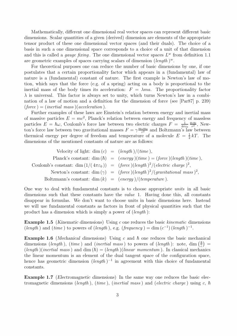
dimensions of the mentioned constants of nature are as follows:

Velocity of light: dim (c) = (length )/(time ),

Planck’s constant: dim (~) = (energy )(time ) = (force )(length )(time ),

Coulomb’s constant: dim (1/( 4πε0 )) = (force )(length )2/(electric charge )2,

Newton’s constant: dim (γ) = (force )(length )2/(gravitational mass )2,

Boltzmann’s constant: dim (k) = (energy )/(temperature ).

One way to deal with fundamental constants is to choose appropriate units in all basicdimensions such that these constants have the value 1. Having done this, all constantsdisappear in formulas. We don’t want to choose units in basic dimensions here. Insteadwe will use fundamental constants as factors in front of physical quantities such that theproduct has a dimension which is simply a power of (length ):

Example 1.5 (Kinematic dimensions) Using c one reduces the basic kinematic dimensions(length ) and (time ) to powers of (length ), e.g. (frequency ) = dim (c−1) (length )−1.

Example 1.6 (Mechanical dimensions) Using c and ~ one reduces the basic mechanicaldimensions (length ), (time ) and (inertial mass ) to powers of (length ): note, dim

(~

c

)=

(length )(inertial mass ) and dim (~) = (length )(linear momentum ). In classical mechanicsthe linear momentum is an element of the dual tangent space of the configuration space,hence has geometric dimension (length )−1 in agreement with this choice of fundamentalconstants.

Example 1.7 (Electromagnetic dimensions) In the same way one reduces the basic elec-tromagnetic dimensions (length ), (time ), (inertial mass ) and (electric charge ) using c, ~

3

and 14πε0

to powers of (length ). Notice that dim (~c) = (force )(length )2 and hence there is

a natural unit for electric charges since (electric charge )2 = ~c 4πε0 and electric charge qbecomes dimensionless (i.e. a real number) when divided by

√~c 4πε0 .

In electrostatics there are two basic quantities. The electric field strength E has di-mension dim (E) = (force )/(electric charge ). The dielectric displacement D has dimensiondim (D) = (electric charge )/(area ). Notice,

dim

(√4πε0

~cE

)= dim

(√1

4πε0 ~cD

)= (length )−2.

In magnetostatics there are also two basic quantities. It is convenient to introduce the di-mensions (current ) := (electric charge )/(time ) and (voltage ) := (energy )/(electric charge ).The magnetic flux B has dimension dim (B) = (voltage )(time )/(area ) and the magneticloop tension H has dimension dim (H) = (current )/(length ). Notice once more,

dim

(√4πε0 c

~B

)= dim

(√1

4πε0 ~c3H

)= (length )−2.

In relativistic electromagnetism, the electric field E and the magnetic flux B are sum-marized into a 2-form F , the so called Faraday form F . The first Maxwell equation dF = 0is expressed in terms of the natural exterior derivative see paragraphs 1.23 and 2.9. TheFaraday form therefore carries the geometric dimension (length )−2. Similarly, the dielectricdisplacement D and the magnetic loop tension H are summarized into a bivector density(denoted by G). The second Maxwell equation is expressed in terms of the natural exteriordivergence see paragraphs 1.24 and 2.9. The bivector density G therefore carries the geo-metric dimension (length )2−n, where n is the spacetime dimension. Hence with the abovechoice of fundamental constants and in n = 4 spacetime dimensions, the natural geometricdimensions and the physical dimensions are in full correspondence.

Example 1.8 (Gravitational dimensions) Analogously, using c, ~ and γ one reduces thebasic gravitational dimensions (length ), (time ), (inertial mass ) and (gravitational mass )to powers of (length ). A gravitational mass becomes dimensionless, when divided by

√~c/γ.

Example 1.9 (Thermodynamical dimensions) Using c, ~ and k one reduces the basic ther-modynamical dimensions (length ), (time ), (inertial mass ) and (temperature ) to powers of(length ).

Fundamental constants as factors allow scalars of any physical dimension to be viewed aselements in one of the geometrically defined spaces Lw of the previous chapter. Similarly, atensorial physical quantity is mathematically described by an element in the correspondingtensor space of the central weight according to its dimension.

Remark 1.10 The elementary electric charge e of the electron defines another natural unitof dimension (electric charge ). Hence the quotient e2/(~c 4πε0 ) determines a (dimensionless)real number, the so called electric fine structure constant . A gravitational analogue to anelementary electric charge has not been observed. We will not use the elementary electriccharge of the electron as a unit.

4

Remark 1.11 The equivalence principle formulated as the proportionality between inertialand gravitational mass of a massive particle leads to another constant which one could callGalilei’s constant g:

Galilei’s constant: dim (g) = (gravitational mass )/(inertial mass ).

For historical reasons, this constant is always set to unity (the common units for inertialmass are also used for gravitational mass). Using Galilei’s constant g together with c, ~

and γ Planck found natural units for all dimensions involved, in particular dim (g2~γc−3) =(length )2. We will not make use of the equivalence principle in that way, hence we will notuse Galilei’s constant and we will not use the resulting units of Planck. (We believe thatGalilei’s constant is not fundamental, instead it we would like to view it as a consequence ofa proper understanding of Mach’s principle.)

Remark 1.12 In Einstein’s theory of gravity one usually uses c, γ and Galilei’s constant gfrom above without Planck’s constant ~ to reduce the basic gravitational dimensions to pow-ers of (length ) (see [MW57], p. 596). With this choice of constants we have dim (gγc−2) =(length )/(gravitational mass ) instead of a natural unit for gravitational mass. Taking alsoCoulomb’s electric constant 1/( 4πε0 ) into account, one finds for electric charge in analogy

to gravitational mass dim(gc−2

√γ/( 4πε0 )

)= (length )/(electric charge ). Note that in

this case the electric field strength has dimension dim(gc−2√γ 4πε0E

)= (length )−1, so

that we would lose the correspondence between physical dimensions and natural geometricdimensions explained in paragraph 1.7.

1.3 Density bundles and divergence operators

Applying the construction in definition 1.1 of densities of weight w pointwise to the tangentspace of a n-dimensional manifold M leads to a family of natural real line bundles Lw =Lw(TM) over M . Alternatively one could use the (first order) frame bundle GL (M) of Mand the associated bundle construction for the representation | det |w/n of GL (Rn) to obtain:Lw(TM) = GL (M)×| det |w/n R. These line bundles are oriented and hence trivializable, butexcept for w = 0 do not carry a natural trivialization. The sections of L−n over M play therole of natural integrands. We will follow Calderbank [Cal96] to define natural adjoints ofdifferential operators and distributions. We apply this definition to the deRham complex toobtain the complex of exterior divergences.

Discussion 1.13 (Integration) We fix a notion of integration of smooth functions definedon a unit cube [0, 1]n in Euclidean n-space which satisfies linearity and the transformationformula under diffeomorphisms of the cube to itself. If F : [0, 1]n → M is smooth andµ ∈ C∞(M,L−n) is a density of weight −n then x ∈ [0, 1]n and (F ∗µ)x := µF (x)(∂Fx(.)∧ . . .∧∂Fx(.)) define a density on Rn. We say a real valued R-linear functional

∫M

: C∞o (M,L−n)→

R from densities of weight −n with compact support locally agrees with the Euclidean integralif for any F : [0, 1]n →M and any µ ∈ C∞

o (M,L−n) with supp(µ) ⊂ im (F ) we have:∫

M

µ =

∫

[0,1]nF ∗µ(e1 ∧ . . . ∧ en),

5

where ei is the standard basis in Rn. A partition of unity argument shows existence:

Proposition 1.14 There is a linear functional∫M

: C∞o (M,L−n) → R which locally agrees

with the Euclidean integral and which therefore is unique and invariant under diffeomor-phisms of M .

Discussion 1.15 (Divergence of vector fields) Let X ∈ C∞(M,TM) be a vector field andµ ∈ C∞(M,L−n) a positive density of weight −n. The Lie derivative LXµ is defined bydifferentiating the pull back of µ by the local flow of X. The divergence of X with respectto µ is a function on M defined by (divµX)µ = LXµ. The divergence can be interpreted asthe rate of volume expansion of the flow of X with respect to µ. Notice that for any functionf ∈ C∞(M,R) we have L(fX)µ = LX(fµ), such that the above formula defines a linear firstorder differential operator on vector field densities like µ⊗X:

div : C∞(M,L−n ⊗ TM)→ C∞(M,L−n).

A vector fieldX ∈ C∞o (M,TM) with compact support on the interior ofM has a complete

flow. The diffeomorphism-invariance of the integral leads to the following vanishing result:

Proposition 1.16 (Integration by parts) If X ∈ C∞o (M,TM) has compact support and

µ ∈ C∞(M,L−n) is positive then∫M

div(µ⊗X) = 0.

Definitions 1.17 (Jets, differential operators and pairings) Let EM → M be a vectorbundle. At a point x ∈M we define for any k ∈ N the vector space of sections which vanish upto order k at x to be Zk

x(EM) := {e ∈ C∞(M,EM) | e(x) = 0, de(X) = 0, . . . , dke(x) = 0}.The projection jetk(e)x of a section e ∈ C∞(M,EM) onto the quotient Jetk(EM)x :=C∞(M,EM)/Zk

x(EM) is called the k-jet of e at x . The vector bundle Jet k(EM) → M iscalled the k-jet bundle of EM . We have a bundle inclusion Sym kT ∗ ⊗ EM → Jetk(EM)defined at x ∈ M by a function f ∈ C∞(M,R) with f(x) = 0 as (∂f)k ⊗ e 7→ jetk(f ke).This is the beginning of a short exact sequence of bundle maps:

0→ Sym kT ∗ ⊗ EM → Jetk(EM)→ Jetk−1(EM)→ 0.

Let FM → M denote another vector bundle. A linear differential operator of order k is aR-linear map

∇ : C∞(M,EM)→ C∞(M,FM)

which factors through a bundle map π : Jet k(EM) → FM as ∇ = π ◦ jetk with nonzerosymbol defined to be the composite: Sym kT ∗ ⊗ EM → Jetk(EM) → FM . The universalk-jet operator jetk : C∞(M,EM) → C∞(M, Jetk(EM)) is a particular example. Similarlywe call a R-bilinear map

X : C∞(M,E1M)× C∞(M,E2M)→ C∞(M,FM)

which factors through a bundle map Q : Jet k(E1M) ⊗ Jetk(E2M) → FM as X(e1, e2) =Q(jetk(e1)⊗ jetk(e2)) a bilinear differential pairing of order k .

6

Discussion 1.18 (Adjoints) Let EM → M and FM → M be two vector bundles overM and ∇ : C∞(M,EM) → C∞(M,FM) be a linear differential operator. A differentialoperator ∇∗ : C∞(M,L−n ⊗ F ∗M) → C∞(M,L−n ⊗ E∗M) is called adjoint to ∇, if for allsections with compact support in the interior of M we have

∫M〈∇ e, φ〉 =

∫M〈e,∇∗ φ〉. If

∇∗ exists, it is unique. One way to proof adjointness of two given operators ∇ and ∇∗ is toconstruct a bilinear differential pairing

X∇ : C∞(M,EM)× C∞(M,L−n ⊗ F ∗M)→ C∞(M,L−n ⊗ TM),

such that a divergence formula holds:

div(X∇(e, φ)) = 〈∇ e, φ〉 − 〈e,∇∗ φ〉.

The differential order of the pairing is one less then the order of the operator. In particularfor first order operators the pairing is tensorial.

Definition 1.19 (Covariant derivative) A linear first order operator D : C∞(M,EM) →C∞(M,T ∗⊗EM) with symbol given by the identity on T ∗⊗EM is called covariant derivativeon EM .

Associated to a covariant derivative D is the Riemann curvature tensor RD . It definesthe local obstruction against the existence of parallel sections:

Proposition 1.20 (Curvature) Let D be a covariant derivative of a vector bundle EM . Thefollowing trilinear differential pairing RD : C∞(M,TM) ⊗ C∞(M,TM) ⊗ C∞(M,EM) →C∞(M,EM) defined by RD(X, Y )e := DX(DY e) − DY (DXe) − D[X,Y ]e (where X, Y arevector fields, e a section and the Lie bracket on functions is defined by ∂[X,Y ] = ∂X∂Y −∂Y ∂X)is indeed zero order and defines the curvature of D to be an endomorphism valued 2-formRD ∈ C∞(M,Λ2T ∗ ⊗ E∗ ⊗ EM).

Remark 1.21 A covariant derivative on EM induces a covariant derivative on the dualbundle E∗M by the product rule: ∂X(〈η, e〉) = 〈DXη, e〉 + 〈η,DXe〉, with a vector fieldX and sections e ∈ C∞(M,EM) and η ∈ C∞(M,E∗M). Consider the tensorial pairingEM ⊗ (L−n⊗ T ⊗E∗M)→ L−n⊗TM with e⊗Y ⊗ η 7→ Y 〈e, η〉. It satisfies the divergenceformula:

div(〈e, (Y ⊗ η)〉) = 〈DY e, η〉+ 〈e,DY η〉+ 〈e, η〉 div(Y ),

with Y ∈ C∞(M,L−n ⊗ TM). This shows that a covariant derivative has an adjointD∗ : C∞(M,L−n ⊗ T ⊗ E∗M) → C∞(M,L−n ⊗ E∗M) given by D∗(Y ⊗ η) = −DY η −div(Y )⊗ η.

Discussion 1.22 (Distributions) Let M be a n-dimensional manifold and EM → Ma vector bundle. The space of test functions C∞

o (M,L−n ⊗ E∗M) consists of smoothsections with compact support in the interior of M . The space of sections of the k-jetbundle C∞

o (M, Jetk(L−n ⊗ E∗M)) is equipped with the compact open topology and thispulls back under jetk : C∞

o (M,L−n ⊗ E∗M) → C∞(M, Jetk(L−n ⊗ E∗M)) to induce theCk-topology on C∞

o (M,L−n ⊗ E∗M). A distributional section of EM is a linear map

7

C∞o (M,L−n⊗E∗M)→ R which is continuous with respect to the Ck-topology for all k ∈ N.

The set of all such distributions is denoted by D(M,EM) := C∞o (M,L−n⊗E∗M)∗. Locally

integrable sections of EM , i.e. elements of L1local(M,EM) define distributions via pointwise

contraction and integration over M .Let ∇ : C∞(M,EM) → C∞(M,FM) be a linear differential operator. Its transpose in

terms of distributions always exists: ∇trans : D(M,L−n ⊗ F ∗M) → D(M,L−n ⊗ E∗M). Ifthe restriction of ∇trans to smooth sections gives smooth sections, then this restriction is theadjoint ∇∗ : C∞(M,L−n⊗F ∗M)→ C∞(M,L−n⊗E∗M). If this adjoint exists the operator

∇ can be extended to distributional sections ∇ : D(M,EM) → D(M,FM) via 〈〈∇ e, φ〉〉 =〈〈e,∇∗ φ〉〉 with a distribution e ∈ D(M,EM) and a test function φ ∈ C∞

o (M,L−n ⊗ F ∗M).Since a covariant derivative D of EM always has an adjoint, one can say that distribution

can infinitely often be differentiated.

Discussion 1.23 (Exterior derivative) On any manifold the exterior derivative on alternat-ing forms

d : C∞(M,ΛkT ∗M)→ C∞(M,Λk+1T ∗M)

defines a linear first order differential operator. The sequence of exterior derivatives buildsthe deRham complex : d ◦ d = 0. The resulting cohomology is called deRham cohomology .The deRham complex is locally exact in the sense that it becomes exact when restricted toa contractible open subset of M . The wedge product is a zero order bilinear pairing:

∧ : C∞(M,ΛkT ∗M)× C∞(M,ΛlT ∗M)→ C∞(M,Λk+lT ∗M),

subject to the following Leibniz rule :

d(α ∧ β) = dα ∧ β + (−1)kα ∧ dβ.

Hence the wedge product induces a cup product in the deRham cohomology.

For a vector space V we have a GL (V )-equivariant pairing 〈 , 〉 : ΛkV ∗ ⊗ ΛkV → R.We define interior multiplication by forms to be a linear map y : ΛkV ∗ ⊗ Λk+lV → ΛlVwhich is adjoint to the wedge product in the sense 〈α y a, β〉 = 〈a, α ∧ β〉, with α ∈ ΛkV ∗,a ∈ Λk+lV and β ∈ ΛlV . Similarly interior multiplication by multivectors is a linear mapy : ΛkV ⊗ Λk+lV ∗ → ΛlV ∗. On a n-dimensional manifold M the bundle of alternatingforms can be tensored with the bundle of pseudoscalars L−n⊗ΛnTM and the above interiormultiplication provides an isomorphism

ΛkT ∗ ⊗ (L−n ⊗ ΛnT )∼=−→ L−n ⊗ Λn−kT

α⊗ or 7→ α y or

to obtain the bundle of multivector densities. Likewise we can tensor the bundle of multivec-tor densities by the (dual) pseudoscalars Ln ⊗ ΛnT ∗M to recover the bundle of alternatingforms:

L−n ⊗ ΛkT ⊗ (Ln ⊗ ΛnT ∗)∼=−→ Λn−kT ∗

a⊗ or∗ 7→ a y or∗.

8

Discussion 1.24 (Exterior divergence) The bundle of dual pseudoscalar Ln⊗ΛnT ∗M overM has rank one, comes with a natural norm and hence with local sections or∗ which areparallel. The exterior divergence on multivector densities

div : C∞(M,L−n ⊗ ΛkTM)→ C∞(M,L−n ⊗ Λk−1TM),

is then defined in terms of the exterior derivative by

(div a) y or∗ := (−1)k+1d(a y or∗).

The sequence of divergences defines a complex div ◦ div = 0. The resulting homology iscalled deRham homology . Interior multiplication y is a zero order pairing

y : C∞(M,ΛkT ∗M)× C∞(M,L−n ⊗ Λk+lTM)→ C∞(M,L−nΛlTM).

For α ∈ C∞(M,ΛkT ∗M) and a ∈ C∞(M,L−n ⊗ Λk+lTM) we get from the Leibniz rule thefollowing divergence formula:

(−1)k div(α y a) = dα y a+ α ydiv a.

For that note (α y a) y or∗ = (−1)k(k+l+1)α ∧ (a y or∗). Hence the interior multiplicationdefines a cap product between deRham cohomology and homology. For l = 1 the abovedivergence formula shows that d and − div are adjoints.

Remark 1.25 For k = 0 we recover the divergence on vector fields from paragraph 1.15,since for functions f ∈ C∞(M,R) and vector fields X ∈ C∞(M,L−n⊗ TM) we clearly havethe divergence formula div(fX) = 〈df,X〉+ f div X.

Remark 1.26 Let D be a torsion-free covariant derivative of TM (see definition 1.19 andproposition 2.27). (Local coordinates induce torsion-free derivatives.) With a dual basis ti,θi of TM we like the exterior derivative on a form α to be dα =

∑i θ

i∧Dtiα. With the abovesign convention we obtain for a multivector a applied to the divergence div a =

∑i θ

i yDtia.

Remark 1.27 The divergence operator can also be defined invariantly on decomposablemultivector density fields using the Lie derivative: for k = 1 let µ denote a nonvanishingdensity of weight −n and X, Y vector fields then div(µ⊗X ∧ Y ) = (LXµ)⊗ Y − (LY µ)⊗X + µ⊗ [X, Y ].

Application 1.28 (Covariant exterior derivative) Let EM be again a vector bundle over MandD a covariant derivative on EM . Since the exterior derivative on forms is first order it canbe twisted by D to obtain a sequence of first order differential operators dD : C∞(M,ΛkT ∗⊗EM) → C∞(M,Λk+1T ∗ ⊗ EM) between forms with values in EM . As an example, if X,Y denote vector fields and α a 1-form with values in EM then dDα(X, Y ) := DX(α(Y ))−DY (α(X))− α([X, Y ]). The obstruction for the twisted deRham sequence to be a complexis the Riemann curvature: RD ∈ C∞(Λ2T ∗ ⊗ gl(EM)) which acts on a k-form to give a(k + 2)-form as

dD ◦ dDα =1

2

∑

i,j

θi ∧ θj ∧ RD(ti, tj)α =: RD ∧ α,

9

where ti, θi is a dual basis of TM . Clearly D induces also a derivative on gl(EM) and the

Leibniz rule gives

dD ◦ (dD ◦ dD)α = dDRD ∧ α + (−1)2RD ∧ dDα = dDRD ∧ α + (dD ◦ dD) ◦ dDα.

This observation proves the following (see e.g. [BGV91]):

Proposition 1.29 (Bianchi identity) The curvature tensor RD of a covariant derivative Don EM satisfies a first order integrability condition: 0 = dDRD.

1.4 Orientations and integration over submanifolds

We recall that the one dimensional space of pseudoscalars L−n(V )⊗ΛnV of a n-dimensionalreal vector space V comes with a natural norm |µ ⊗ v| = |µ(v)|. The two unit elementscorrespond to the two orientations of V : if v := t1 ∧ . . . ∧ tn with ti ∈ V is a positive basisof V then this induces or = µ ⊗ v with 0 < µ determined by µ(v) = 1. A unit elementor ∈ L−n(V ) ⊗ ΛnV induces a unique element or∗ ∈ Ln(V ) ⊗ ΛnV ∗ in the dual space by〈or∗, or〉 = 1. Alternatively, the above norm in the one dimensional space L−n(V ) ⊗ ΛnVinduces an inner product, which identifies it with its dual space: L−n(V )⊗ΛnV = Ln(V )⊗ΛnV ∗

Definition 1.30 (Orientation) A vector bundle EM → M of rank k over a n-dimensionalmanifold M is called orientable if the bundle of pseudoscalars L−k(EM)⊗ΛkEM is trivial-izable, i.e. if there is a global section or ∈ C∞(M,L−k(EM)⊗ΛkEM) of norm one |or| = 1.A choice of such a trivialization on an orientable bundle is called an orientation of EM andEM with such a choice is called oriented .

Remark 1.31 In general, if M is connected and x ∈ M a point then there is a group ho-momorphism π1(M,x) → {+1,−1} between the fundamental group and O (R) = {+1,−1}induced by parallel transport in L−k(EM) ⊗ ΛkEM . This homomorphism factors throughthe maximal Abelian quotient π1(M,x)Ab, hence the homomorphism corresponds to a co-homology class w1(EM) ∈ H1(M,Z/2Z). The vector bundle is orientable, iff this class istrivial. In particular if M is simply connected, π1(M,x) = 1, any vector bundle over M isorientable.

Definition 1.32 (Orientation and coorientation) Let S ↪→ M denote a k-dimensional im-mersed submanifold inside a n-dimensional manifold M . The submanifold S ↪→M is calledorientable iff its tangent bundle TS → S is orientable. The submanifold S ↪→ M is calledcoorientable iff the normal bundle (quotient bundle) TM/TS → S is orientable.

Remark 1.33 Points in M are always oriented and the manifold M itself is always coori-ented. The conventional (co)orientations are often denoted by +1, and the opposite orien-tation is denoted by −1.

10

Application 1.34 (Integration over oriented submanifolds) Let S ↪→ M by an immersionas in definition 1.32. If S is orientable and or a choice of orientation then any k-form F onM can be turned into a density 〈F, or〉 ∈ C∞(S, L−k(TS)) over S by means of the followingcontraction:

L−k(TS)⊗ ΛkTS ⊗ ΛkT ∗M → L−k(TS).

Hence 〈F, or〉 can be integrated naturally over S.

Proposition 1.35 If 0 → U → V → V/U → 0 is a short exact sequence of real vectorspaces U , V and V/U , then orientations of two of them induces an orientation of the third.Indeed if k = dim (U) denote the dimension we have the following canonical isomorphismsbetween one dimensional spaces:

L−k(U)⊗ ΛkU ⊗ L−(n−k)(V/U)⊗ Λn−k(V/U)∼=−→ L−n(V )⊗ ΛnV ,

ΛkU ⊗ Λn−k(V/U)∼=−→ ΛnV ,

L−k(U)⊗ L−(n−k)(V/U)∼=−→ L−n(V ).

Application 1.36 (Integration over cooriented submanifolds) Let S ↪→ M denote an im-mersion as in definition 1.32. If S is coorientable and coor ∈ C∞(M,Ln−k(TM/TS) ⊗Λn−k(TM/TS)∗) a choice of coorientation then any (n−k)-multivector density G on M canbe turned into a density 〈G, coor〉 ∈ C∞(S, L−k(TS)) over S, by means of the following map(we will use the notation TS⊥ = (TM/TS)∗):

L−n(TM)⊗ Λn−kTM ⊗ Ln−k(TM/TS)⊗ Λn−kTS⊥ → L−n(TM)⊗ Ln−k(TM/TS)∼= L−k(TS).

Hence 〈G, coor〉 can be integrated naturally over S.

Application 1.37 (Outer normal) If S is a manifold with boundary ∂S then the outernormal induces an orientation of the normal bundle of the boundary out ∈ L−1(TS/T∂S)⊗Λ1(TS/T∂S) with |out| = 1 along ∂S. Applying the proposition 1.35 for 0→ T∂S → TS →TS/T∂S → 0 and for 0 → TS/T∂S → TM/T∂S → TM/TS → 0 we have two inducedisomorphisms:

L−k(TS)⊗ Λk(TS) → L1−k(T∂S)⊗ Λk−1(T∂S),

Ln−k(TM/TS)⊗ Λn−k(TS)⊥ → Ln+1−k(TM/T∂S)⊗ Λn+1−k(T∂S)⊥.

Hence a (co-)orientation of S induces a (co-)orientation of ∂S.

Proposition 1.38 (Stoke’s theorem) If F ∈ C∞(M,ΛkT ∗M) is a smooth k-form on a n-manifold M , and Σ ↪→M an (immersed) compact oriented (k+ 1)-dimensional submanifoldwith boundary ∂Σ then ∫

∂Σ

〈F, or〉 =

∫

Σ

〈dF, or〉.

11

Proposition 1.39 (Divergence theorem) If G ∈ C∞(M,L−n⊗Λn−kTM) is a smooth (n−k)-multivector density on an n-manifold M , and Σ ↪→M an (immersed) compact cooriented(k + 1)-dimensional submanifold with boundary ∂Σ then

∫

∂Σ

〈G, coor〉 =

∫

Σ

〈div G, coor〉.

Remark 1.40 In the case of M being a manifold with boundary ∂M the outer normalalways induces a coorientation of ∂M and M itself is always cooriented. Hence the abovedivergence theorem applies to the whole of M without any orientability assumptions whichis called Gauß theorem , whereas Stoke’s theorem needs an orientable M .

1.5 Scale invariance in functional analysis

In real functional analysis the weight in definition 1.1 is related to the so called Sobolevnumber . To demonstrate this relation we will briefly recall Lebesgue and Sobolev spacesusing density valued functions. The dimensional analysis then gives an explanation of theHolder and Sobolev inequalities. Recall that the integral of a sections of the line bundle L−n

over a n-dimensional compact domain is invariant under diffeomorphisms of the domain.

Discussion 1.41 (Lebesgue spaces) A scalar function lives in the Lebesgue space Lp forsome p ∈ R if the pth power of its modulus is integrable. Therefore such a scalar functionshould be considered as a section of L−n/p, i.e. one assigns −n/p as the weight of thatfunction. Hence Lp can be called the space of integrable functions of weight w = −n/p . For0 < w (i.e. p < 0) this space of functions fails to be a vector space (local problem) and forw < −n (i.e. 0 ≤ p < 1) it fails to satisfy the triangle inequality. Therefore a natural rangefor w is −n ≤ w ≤ 0. We may denote the norm of an integrable function u of weight w by

||u||(w) :=

∫|u|−n/w.

Holder’s inequality implies that the product of two integrable functions of weight w1 and w2

respectively is integrable of weight w1 + w2.

Discussion 1.42 (Sobolev spaces) If a function has weight w then its kth derivative willhave weight w − k. If a function lives in the Sobolev space Wk,p then in particular its kthderivative is in Lp. Hence it is natural to assign w with w − k = −n/p as the weight ofthat function; w the equals the Sobolev number w = k − n/p. For a compact domain withsmooth boundary and in the case of the first derivative k = 1 we reformulate Sobolev’s andHolder’s inequality in terms of weights as follows: for (1 − n) ≤ w < 0 we have Sobolev’sinequality:

||u||(w) ≤ C(n, w)||∂u||(w−1),

with a constant C(n, w) depending on the domain and the weight w, similarly for 0 < w ≤ 1we have the Holder estimate:

|u(x)− u(y)| ≤ C(n, w)|x− y|w||∂u||(w−1).

Note how the dimensional analysis takes care of the correct exponents.

12

Example 1.43 If a differential operator ∇ of order k is selfadjoint then the pointwise innerproduct 〈∇φ, ψ〉 should be considered as a density of weight −n (since these are the naturalintegrands) leaving w = (k−n)/2 as natural weight for φ and ψ. This weight coincides withthe Sobolev number of the space Wk/2,2 which is the usual domain of ∇ in terms of its weakformulation.

If a partial differential equation has a geometric origin, the involved unknown functionmay have a natural geometric dimension (length )w. Such a natural or geometric weight wusually equals the critical Sobolev number , i.e. natural sections just fail to be integrable.(For example the Euclidean distance dist(Σ, .) to a submanifold Σ is geometrically given bya section of L1 which is always critical.)

Example 1.44 The Yamabe problem of finding a metric within a given conformal classwhich has constant scalar curvature (with respect to its own length scale) is a typical exampleof such a situation. The problem reduces to a nonlinear eigenvalue problem for the conformalLaplace operator (see example 4.47) ∆f (2−n)/2 = −f (−2−n)/2 with normalization

∫f−n = 1,

where f is a positive section of L1 playing the role of a length scale. The geometric contexthas already determined the Laplace operator to act on densities of weight w = (2 − n)/2,which agrees with the Sobolev number in the usual analytic setting in W1,2, see [LP87].

1.6 Weyl derivatives

Since the density line bundles Lw over a manifold M have no preferred trivialization (exceptfor w = 0) covariant derivatives on these line bundles are of differential geometric interest.We will indicate how densities and Weyl derivatives provide a way to geometrize electromag-netism. Any first order differential operator can be twisted by a Weyl derivative to definean operator on sections of arbitrary central weight. We apply this to the deRham complexand its adjoint.

Definition 1.45 (Weyl derivatives) A covariant derivative D of L1 is called a Weyl deriva-tive (see definition 1.19). It naturally induces covariant derivatives on all density bundlesLw (e.g. by means of parallel transport).

Definition 1.46 (Faraday curvature) The curvature (see proposition 1.20) of a Weyl deriva-tive D in L1 is an endomorphism valued 2-form which for a line bundle is determined by areal valued 2-form FD ∈ C∞(M,Λ2T ∗M).

The differential Bianchi identity, see proposition 1.29, applied to a given Weyl deriva-tive D means that FD is a closed 2-form, dFD = 0. Originally Weyl interpreted a Weylderivative as electromagnetic potential and its curvature as electromagnetic field, which thenautomatically satisfies the first Maxwell equation. Therefore we like to call the closed twoform FD the Faraday curvature . The induced curvature of Lw is given by wFD.

The Faraday curvature is the local obstruction for finding a parallel trivialization of L1.The Weyl derivative D is called closed if FD = 0. For a closed Weyl derivative one can findlocally positive sections of L1, which are D parallel. If there is a global positive D parallel

13

section µ of L1 then D is called exact . Conversely a positive section of L1 determines anexact Weyl derivative Dµ via Dµµ = 0.

The space of all Weyl derivatives forms an affine space modelled on the linear space ofsmooth 1-forms C∞(M,T ∗M): let D and D be two covariant derivatives in the line bundle

L1. They differ by an endomorphism valued 1-form D−D = γ which for a line bundle is justa real valued 1-form γ ∈ C∞(M,T ∗M). The induced derivatives in Lk differ by D−D = kγ.Closed and exact Weyl derivatives are affine subspaces modelled on closed and exact 1-formsrespectively.

Application 1.47 (Twisted exterior derivative) With the help of a Weyl derivative D theexterior derivative d can be extended to forms of arbitrary central weight (see paragraph1.28):

dD : C∞(M,Lw ⊗ ΛkT ∗M)→ C∞(M,Lw ⊗ Λk+1T ∗M).

The obstruction for the twisted deRham sequence to be a complex is the Faraday curvatureFD.

Application 1.48 (Twisted exterior divergence) Similarly a Weyl derivative D defines di-vergences on multivector field densities of arbitrary central weight

divD : C∞(M,Lw−n ⊗ ΛkTM)→ C∞(M,Lw−n ⊗ Λk−1TM).

For example if µ denotes a density of weight w and X a vector field of central weight 1− n,then divD(µ⊗X) = tr(Dµ⊗X) + µ⊗ div X.

Remark 1.49 Lie derivative, Weyl derivative and twisted divergence are related as follows:for a density µ of weight w and a vector field K we have LKµ = DKµ− w

nµ divDK.

The vector field K generates diffeomorphisms which leave a given Weyl derivative Dinvariant, iff it satisfies the following linear partial differential equation of second order:0 = LKD. Here LKD denotes a real valued 1-form defined with the help of vector field Xand a length scale µ ∈ L1 by

(LKD)Xµ = LK(DXµ)−DLKXµ−DX(LKµ)

= FD(K,X)µ+1

nµ ∂X(divDK).

14

Chapter 2

Elementary conformal geometry

This chapter provides the elementary background in relativity, representation theory anddifferential geometry which we will use in the sequel. In the first two sections we define aconformal structure on a vector space and apply this to relativistic kinematics and electro-magnetism in Minkowski space. The freedom of choosing a particular inner product in theconformal class corresponds to the free choice of a unit for the dimension (length ). Lightrays, relative velocity of observers, conservation of momentum in collision experiments andthe electromagnetic constitutive relation in vacuum only depend upon a conformal structure.Perihelion advance illustrates the impact of special relativity on the motion in a central forcefield. In section 2.3 we recall how manifolds can be equipped with a conformal structure.There is no preferred covariant derivative on a conformal manifold: instead the space ofWeyl derivatives parameterizes compatible derivatives of the tangent bundle. In sections2.4 and 2.5 we recall how vector bundles are associated to the orthogonal frame bundle anddetermine their curvature properties. In section 2.6 we adapt Branson’s method to Weylderivatives, which reduces the question of conformal invariance to a linear question. In thelast section we recall the first few integrability conditions of the conformal curvature tensors.These Bianchi identities motivate the field equations for Einstein’s and Bach’s theories ofgravity.

2.1 Conformal vector spaces

Conformal geometry concerns the concept of angle without that of absolute length. Aconformal structure of a vector space is an equivalence class of inner products with the samenotion of orthogonality. Hence two such inner products differ by a multiplicative factor infront. Since there is no preferred inner product in the class we give the following invariantdefinition which is taken from [Cal98b]:

Definition 2.1 (Conformal vector space) A conformal structure c of a real vector space Vis a normalized inner product on the weightless space L−1 ⊗ V . Normalized means that onΛn(L−1 ⊗ V ) = L−n ⊗ΛnV the canonical inner product and the inner product induced by c

coincide: | det c| = 1. Alternatively c can be viewed as a normalized L2 valued inner producton V . If A is an affine space over the conformal vector space V then A carries a conformal

15

structure.

Remark 2.2 A conformal structure can also be defined as an equivalence class of innerproducts: a positive element µ ∈ L1 is called a length scale and it determines by µ−2

c a (realvalued) inner product on V with µ−n as volume density. On the other hand, given a (realvalued) inner product g on V then g represents a conformal structure given by c := µ(g)2g,where µ(g) is the length scale of g (equivalently µ−n(g) is the volume density of g).

Notation 2.3 We will use the conformal metric to identify V with its dual, precisely, wewill use the isomorphisms ] : Lk ⊗ V ∗ → Lk−2 ⊗ V and [ : Lk ⊗ V → Lk+2 ⊗ V ∗ sometimeswithout denoting them.

The following remark is a bit technical. We will use it to integrate sections in L−1 alongnonlightlike curves (application 4.26) and to recover the electric field and the magnetic fluxfrom a Faraday 2-form, see remark 2.10.

Remark 2.4 (Pull back of densities) If ι : U → V denotes a subspace of dimension kon which the induced conformal inner product stays nondegenerated, then we have an in-duced map ι∗ : L−k(V ) → L−k(U): for µ ∈ L−k(V ), u ∈ ΛkU , sign(µ) = ±1 we de-fine ι∗(µ)(u) := sign(µ)

√c(µ⊗ ι(u), µ⊗ ι(u)), where c is the induced inner product on

Λk(V 0). More generally for all weights w we have ι∗ : Lw(V ) → Lw(U) with ι∗(µ)(u) =sign(µ)(|(|µ|)−k/w ⊗ u|c)−w/k.

2.2 Special relativity and electromagnetism

The simplest geometrical model of physical spacetime is an affine space A over a real n = 4dimensional vector space V . Points in A are called events and an observer living for sometime traces out a worldline in A. In principle an (infinitesimal) observer v ∈ V along hisworldline can measure the angle between two direction and can decide whether two rulershave equal length (at the same time). Hence (infinitesimal) spacelike measurements takeplace in a conformal class of (Euclidean) metrics (of the three dimensional quotient V/Rv).Note, that the focus on conformal metrics also corresponds to the following physical principle:

Discussion 2.5 (Constant velocity of light) Lightrays travel through spacetime in a waywhich is independent of the motion of the emitter. In the geometrical model these naturallygiven lightrays form double cones through each (emitting) event. In special relativity theselight cones come from a conformal class c of inner products in V with Lorentzian signature(3, 1). Note that such a lightcone {v ∈ V | c(v, v) = 0} characterizes its conformal metric.

The geometry of lightcones describes the causal relation between events:

Definition 2.6 (Causality) Vectors v ∈ V inside the lightcone c(v, v) < 0 of an eventx ∈ A are called timelike , vectors v with c(v, v) > 0 are called spacelike and vectors v withc(v, v) = 0 are called lightlike .

16

Similarly a (piecewise) differentiable path is called timelike (respectively spacelike orlightlike), if all velocity vectors are timelike (respectively spacelike or lightlike). We say thattwo events x and x + v with v timelike are in causal relation . A lightlike or timelike pathjoining two events x and x+ v with v spacelike needs to change its time direction.

Observers are smooth curves c(t) ∈ A with timelike velocity vectors c. The pointsin the intersection of the forward lightcone of c(t0 − τ) with the backward lightcone ofc(t0 + τ) are called simultaneous events relative to c . The three dimensional linear spacec(t0)

⊥ := {v ∈ V | c(v, c(t0)) = 0} perpendicular to c(t0) describes the space of simultaneousevents infinitesimally.

Remark 2.7 (Relative velocity) Relativistic kinematics of particles is also based upon theconformal Lorentzian metric: let U ∈ V 0 := L−1⊗V be a unit tangent vector to a worldlineof an observer, hence U is timelike and normalized c(U, U) = −1, see also 4.10. A secondobserver N with c(N,N) = −1 meeting U at an event x points into the same time directionas U , if c(U,N) < 0. In that case N measures a relative velocity ~u ∈ N⊥ ⊂ V 0 (asmultiple of the velocity of light, example 1.5) in his infinitesimal space of simultaneous eventsc(~u,N) = 0 given by the condition N + ~u ∼ U , hence N + ~u = −U/ c(U,N). Squaring thisequation gives |~u|2 = 1− 1/ c(U,N)2.

Remark 2.8 (Collision experiments) If two (pointlike) bodies collide at an event in space-time then their initial velocities N1 and N2 (weightless and normalized) and inertial massesm1 and m2 are related to their final velocities N ′

1 and N ′2 (weightless and normalized) and

final inertial masses m′1 and m′

2 as m1N1 +m2N2 = m′1N

′1 +m′

2N′2 (see [Par87] p. 18ff). Note

that this conservation law at the (idealized) event of collision only depends upon the confor-mal structure. From the dimensional analysis of example 1.6 we think of inertial masses aselements in L−1 and m1N1 ∈ V ∗ is called the linear momentum of the body.

Electromagnetism deals with the following physical phenomenon: motion of electriccharges produces fields which travel with the speed of light and these fields influence themotion of charged particles . The theory describing electromagnetic interactions is basedupon Maxwell’s equations. In their relativistic form due to Minkowski the field equationsare part of the deRham sequence of the exterior derivative and its adjoint the sequence ofexterior divergences:

Definition 2.9 (Electromagnetic field theory) A vector field j of central weight 1 − nrepresents the charge current density . It plays the role of the source and has to satisfya conservation law : div j = 0. We have to distinguish between two realizations of the fielditself, the dynamic and the kinematic field. The dynamic field G is represented by a bivectordensity field of central weight 2 − n and it is coupled to the source by the second Maxwellequation j = div G. The kinematic field F is represented by a 2-form of central weight−2 the so called Faraday 2-form and satisfies an integrability condition dF = 0 the firstMaxwell equation.

Remark 2.10 (E and B field) Relative to an observer c(N,N) = −1 with its space ofsimultaneous events N⊥ ⊂ V 0 the kinematic field F splits into two tensors of central weight−2 in N⊥. We make secret use of the remark 2.4 and define a 1-form the electric field strength

17

E(~u) := F (N,~u) and a 2-form the magnetic flux B(~u,~v) := F (~u,~v) with ~u,~v ∈ N⊥. Similarlythe dynamic field G splits into the dielectric displacement D(~u) := G(N,~u), a vector on N⊥

of central weight −2 and the magnetic loop tension H(~u,~v) := G(~u,~v) a bivector on N⊥ ofcentral weight −2. For the physical dimensions see example 1.7.

Discussion 2.11 (Constitutive relation) Dynamic and kinematic fields are related by theso called constitutive relation which depends upon the matter in which the field propa-gates. In vacuum (and in n = 4 dimensions) the constitutive relation between F and G issimply given by a conformal structure c of Lorentzian signature (n − 1, 1), i.e. F (X, Y ) =∑

i,j c(X, ti) c(Y, tj)G(θi, θj), where X, Y are vectors and ti, θi is a dual basis of V .

Since the kinematic field F is closed there (locally) exists a 1-form A of central weight−1, called potential , such that F = dA. This potential is not uniquely determined by F ,instead it is subject to (local) transformations A 7→ A + df , where f is a function, called agauge function .

Summary 2.12 To summarize, the electromagnetic field theory in vacuum takes place inan (affine) space modelled on a four dimensional vector space V with conformal metric ofLorentzian signature. The kinematic sequence is given by the beginning of the deRhamsequence of the exterior derivative:

gauge potential kinematic field

C∞(A,R)d→ C∞(A, V ∗)

d→ C∞(A,Λ2V ∗)d→ C∞(A,Λ3V ∗)

f A F 0

The dynamic sequence is given by the end of the sequence of the exterior divergence:

0 j G

C∞(A, L−n)div← C∞(A, L−n ⊗ V )

div← C∞(A, L−n ⊗ Λ2V )div← C∞(A, L−n ⊗ Λ3V )

source dynamic field

The conformal metric is the constitutive relation between kinematic and dynamic field.Hence the Maxwell equations in vacuum are linear and conformally invariant given by:

F = G via the conformal structure c,0 = div j and j = div G,

0 = dF and F = dA and A 7→ A+ df .

Remark 2.13 Note that the second Maxwell equation div G = j between the dynamic fieldand the source already determines all other differential operators which are involved: theintegrability condition for div G = j gives the conservation of the source 0 = div div G =div j, adjoint to this conservation law is the operator for the gauge transformation A+ df ,these transformations are in the kernel of the equation between potential and kinematic fieldF = dA = d(A+df) (which is also adjoint to div G = j), finally the integrability of dA = Fgives the first Maxwell equation 0 = ddA = dF .

18

Discussion 2.14 (Lorentz force law) Galilei’s principle of inertia means that a free massiveparticle with initial velocity N in spacetime has the tendency to stick to that spacetimedirection, i.e. in the affine model of spacetime a free massive particle moves along straighttimelike lines: DNN = 0, where D denotes the affine derivative. Obviously the principle ofinertia isn’t conformally invariant, since it involves the affine derivative. If an electromagneticfield F is present, an electrically charged particle q ∈ R is no longer free, instead it isinfluenced by F : a simple relativistic law of motion is then given by

mDNN = q](F (N)),

where m ∈ L−1 is the inertial mass of the charged particle and N is viewed as a test particle(q/m is small compared to F ).

Example 2.15 (Coulomb field) Coulomb’s (nonrelativistic) law determines the force be-tween two charges q and Q which are at rest relative to the laboratory to be qQ/r2.Viewing one charge q as test particle and the other Q as source, the Lorentz force lawmDNN = qF (N) determines the corresponding Faraday 2-form F which solves Maxwell’sequations - the Coulomb field: let N be the unit timelike vector of the two charges andidentify the conformal affine spacetime A with V by taking an event o ∈ A along thestraight worldline of the source as origin. If P : V → N⊥ ⊂ V denotes the projectionv 7→ v−〈v,N〉/〈N,N〉N the radial distance r : A→ L1 to the source is given by r(c) := |x|,where x = x(c) := P (c − o) ∈ N⊥ is the spacelike location of the test particle. Coulomb’sforce law on the one hand and Lorentz force law on the other hand gives qQ/r2 ~r = qF (N),where ~r = x/|x| = gradD r denotes the unit radial field, which is the gradient of the distancefunction with respect to the (usual) affine derivative D. Therefore if F : A→ Λ2V ∗ is a pureelectric field for N then it is given by

F = FCoul := Q/r2 (〈~r, .〉N − 〈N, .〉~r).

Discussion 2.16 (Motion in a central field) Next we like to study the relativistic motionof a test particle c : R → A subject to the Lorentz force in the Coulomb field. For that wesolve the ordinary differential equation

c = −a/r2 (〈~r, c〉N − 〈N, c〉~r),

where a ∈ R is a number. Clearly 〈c, c〉 is a constant of motion. For the projection x := P (c)we have

x = P (c) = −a/r2(−〈c, N〉)~r.The function −〈c, N〉 satisfies ∂

∂t(−〈c, N〉) = a ∂

∂t(1/r), hence

−〈c, N〉 = b+ a/r,

where b = −〈c(0), N〉−a/r(0) depends on the initial conditions only. Hence we can introducethe central potential U : R+ → R defined by

U(r) := −ab/r − (1

2a2)/r2,

19

and (with U(x) = U(|x|)) the differential equation becomes

x = − grad Ux = −U ′(|x|)x/|x|r(t) = |x(t)|c(t) = x(t) + (b+ a/r(t))N.

We have the usual conserved quantities in a central potential: angular momentum ~l := x∧xwith length squared l2 = 〈x, x〉r2− (rr)2 and energy E := 1

2〈x, x〉+U(|x|) = 1

2r2 + 1

2l2/r2 +

U(r). The conservation of the bivector ~l means that the solution curve for x(t) lies in a planex = r(cos(φ), sin(φ)) and for the polar angle φ we have φ = l/r2. Note 〈c, c〉 = 2E − b2.

Discussion 2.17 (Perihelion advance) In the case of a Coulomb field of a charge Q andan opposite test charge q with inertial mass m we have a = −Qq/m > 0, i.e. an attractivepotential. A timelike solution curve 〈c, c〉 = −1 = 2E − b2 which directs into the same time0 < −〈c, N〉 is guaranteed if b > 0. If in addition −1/2 < E < 0 and a2 < l2 < a2/(−2E) wehave bounded orbits 0 ≤ (r)2 = 2E − 2U(r)− l2/r2 hence rP ≤ r ≤ rA with rA/P = r0 ± q,(−2E)r0 := ab and (−2E)q2 := a2/(−2E)− l2. Since (r)2 = (−2E)(rA − r)(r − rP )/r2 thepolar angle satisfies

φ′(r) =φ

r=

l

r2r=

l√−2E

1

r√

(rA − r)(r − rP ),

hence with φ(rP ) = 0 we find

φ(r) =l√

(−2E)rArParccos

(rP rA − r0r

qr

).

Finally φ(rA) = πl/√

(−2E)rArP and the total angle between two perihelion constellations(moment of nearest approach to the centre) is given by:

2πl√

(−2E)rArP= 2π

1√1− (a/l)2

≈ 2π(1 +1

2(a/l)2 +

3

8(a/l)4 + . . .).

(We could compare the above special relativistic perihelion advance with the perihelionadvance in the Schwarzschild model (see e.g. [ONe83] p. 379): the qualitative behavior issimilar, since the leading term is in both cases given by (a/l)2, but the special relativisticfactor in front is 1

2whereas in the Schwarzschild model it is 3.)

Discussion 2.18 (Charge) In physical situations where a smooth source j models thecharge distribution with a dynamic field G subject to div G = j we deduce from the diver-gence theorem that the integral of j over a cooriented (n− 1)-dimensional ball

∫B〈j, coor〉 =∫

B〈div G, coor〉 =

∫∂B〈G, coor〉 only depends upon the boundary ∂B rather then the span-

ning B. This leads to the definition 2.19 of charge represented by G for the case of G beingsmooth in a region away from supp(j) even if j is distributional. We remark that the integral∫∂B〈G, coor〉 only depends upon the homology class of ∂B as will be explained in proposition

2.20. In what follows we let M ⊂ A be an open region away from supp(j) where the field Gis smooth.

20

Definition 2.19 (Electric charge) If G denotes a smooth divergence-free bivector densitywe define the electric charge (represented by G) contained in an (immersed) cooriented(n− 2)-dimensional sphere Sn−2 ↪→M by:

Qe :=

∫

Sn−2

〈G, coor〉.

As is well known, this quantity satisfies a conservation law, which follows from the diver-gence theorem:

Proposition 2.20 If Sn−2 = ∂Σ is the boundary of an (immersed) compact cooriented(n − 1)-dimensional submanifold Σ ↪→ M , then Qe = 0. Consequently, if Sn−2, coor andSn−2′, coor ′ are two immersed spheres, such that there is an (immersed) compact cooriented(n − 1)-dimensional submanifold Σ, coor with these two spheres as boundary: ∂Σ, coor =Sn−2, coor ∪ Sn−2′,−coor ′, then Sn−2 and Sn−2′ contain the same amount of electric charge.

For completeness we will also define magnetic charge represented by a Faraday 2-form:

Definition 2.21 (Magnetic charge) If F denotes a smooth closed 2-form we define themagnetic charge (represented by F ) contained in an (immersed) oriented 2-dimensionalsphere S2 ↪→M by:

Qm :=

∫

S2

〈F, or〉.

This quantity satisfies a conservation law, which follows from Stoke’s theorem:

Proposition 2.22 If S2 = ∂Σ is the boundary of an (immersed) compact oriented 3-dimensional submanifold Σ ↪→ M , then Qm = 0. Consequently, if S2, or and S2′, or ′ aretwo immersed spheres, such that there is an (immersed) compact oriented 3-dimensionalsubmanifold Σ, or with these two spheres as boundary: ∂Σ, or = S2, or ∪ S2′,−or ′, then S2

and S2′ contain the same amount of magnetic charge.

Remark 2.23 The differential equations of electromagnetism make sense on any conformalmanifold. Source-free electromagnetic fields can then give rise to charge due to nontrivialtopology of the underlying manifold. See the joint article by Hadley and the author [DH99]for a review and extension of this idea.

2.3 Conformal structure on manifolds

In this section we follow Weyl [Wey70], Bergmann and Einstein [Ber76] to define conformalstructures and related geometries on arbitrary smooth manifolds. A Riemannian metricdefines a conformal class of metrics, but there is no preferred metric within such a class.Consequently we define a conformal structure invariantly as a single Riemannian metric ofthe weightless tangent bundle. There is no preferred covariant derivative on a conformalmanifold instead we deal with an affine space of derivatives modelled on the space of smooth1-forms.

21

Definition 2.24 A conformal structure on a manifoldM is a (smooth) normalized L2 valuedinner product c on TM (see definition 2.1). It can be viewed as a nondegenerate normalized(real valued) inner product on the weightless tangent bundle L−1⊗TM . This inner productbetween vector fields X and Y will also be denoted by 〈X, Y 〉 = c(X, Y ).

Definition 2.25 (Conformal geometry) A conformal structure c defines a conformal geom-etry on M . Naively, a construction is called conformally invariant, if it only depends uponc, i.e. if the construction is defined using an additional choice one needs to show that theconstruction is indeed independent of that choice.

Definition 2.26 (Conformal Killing fields) A vector field K on a conformal manifold Mgenerates diffeomorphisms which leave the conformal structure c invariant iff 0 = LKc. Asolution to this linear first order partial differential equation is called a conformal Killingfield .

Proposition 2.27 (Torsion) Let D be a covariant derivative of the tangent bundle TM .The following bilinear differential pairing TD : C∞(M,TM)⊗C∞(M,TM)→ C∞(M,TM)defined by TD(X, Y ) := DXY − DYX − [X, Y ] (where X, Y are vector fields and the Liebracket on functions is defined by ∂[X,Y ] = ∂X∂Y − ∂Y ∂X) is indeed zero order and definesthe torsion of D to be a vector valued 2-form TD ∈ C∞(M,Λ2T ∗ ⊗ TM).

A covariant derivative D on TM is called torsion-free if TD = 0. A covariant derivativeD on TM induces covariant derivatives on all tensor bundles including Lw (for instance bymeans of parallel transport or via the induced connection on the first order frame bundleGL (M)). The covariant derivative on L1 is called a Weyl derivative, see definition 1.45.The derivative D is called compatible with the conformal structure if Dc = 0.

Theorem 2.28 (Fundamental theorem of conformal geometry) On a conformal manifoldMthere is a one to one correspondence between covariant derivatives on L1 and derivatives onTM , which are torsion-free and compatible with the conformal structure c. Such derivativeswill be called Weyl derivatives and for vector fields X,Y ,Z the Koszul formula holds:

2 c(DXY, Z) = DX( c(Y, Z)) +DY ( c(Z,X))−DZ( c(X, Y ))

+ c([X, Y ], Z)− c([Y, Z ], X) + c([Z,X ], Y ).

Proof: The arguments needed here are the same as those used in Riemannian geome-try: first of all if a covariant derivative D is torsion-free and Dc = 0 then the aboveKoszul formula holds. Furthermore, if f ∈ C∞(M,R) is a function then D defined by theKoszul formula satisfies DfXY = fDXY and DX(fY ) = (∂Xf)Y + fDXY since [ fX, Y ] =f [X, Y ]− (∂Y f)X. 2

Definition 2.29 (Riemannian geometry) A length scale, i.e. a positive section µ of L1 plusa conformal structure c defines a Riemannian geometry on M . Let D be the (exact) Weylderivative which leaves the length scale parallel. The induced derivative on TM is then theLevi-Civita derivative of the metric µ−2

c.

22

A vector field K on a n-dimensional manifold M with Riemannian geometry, generatesdiffeomorphisms which leave the geometry invariant, iff K is a conformal Killing field whichleaves the length scale invariant i.e. 0 = LKc and 0 = LKµ. The second condition says thatthe vector field is divergence-free (with respect to the length scale). Using the Levi-Civitaderivative, the two equations can be summarized by saying that DK is a skew symmetricendomorphism field.

Definition 2.30 (Weyl geometry) A Weyl derivative D in L1 plus a conformal structure c

defines a Weyl geometry on M .

A vector field K on a n-dimensional manifold M with Weyl geometry, generates diffeo-morphisms which leave the geometry invariant, iff K is a conformal Killing field which leavesthe Weyl derivative invariant i.e. 0 = LKc and 0 = LKD = FD(K, ) + 1

n∂ divDK. The

conformal Killing equation can be rewritten in terms of the Weyl derivative D:

(LKc)(X, Y ) = LK( c(X, Y ))− c(LKX, Y )− c(X,LKY )

= c(DXK, Y ) + c(X,DYK)− 2

n(divDK) c(X, Y ).

A vector field solving both equations is called a Weyl Killing field . Its 2-jet is alreadydetermined from its 1-jet, since for the induced derivative D on TM we clearly have 0 = LKDand

(LKD)XY = LK(DXY )−DLKXY −DXLKY= DKDXY −DDXYK −D[K,X ]Y −DXDKY +DXDYK

= RDK,XY +D2

X,YK.

Remark 2.31 (Weyl’s unified theory of electromagnetism and gravity) Einstein’s theoryof gravity models the spacetime by a four dimensional manifold M with a Lorentzian metricg. Its divergence-free Ricci curvature, see remark 2.63, is coupled to the energy density ofthe matter in question. Electromagnetism is then modelled by an additional field F on M(which might contribute to the matter energy). In contradistinction Weyl geometry providesa geometric model of spacetime where the electromagnetic field is intrinsically representedby the Faraday curvature FD, see [Wey70] and the next remark 2.32.

Remark 2.32 (Twin paradox) In case of Weyl geometry with Lorentzian signature we saythat the parameterization of a timelike worldline c : R → M is proportional to the propertime of the observer c if 〈Dcc, c〉 = 0. If two different worldlines c1 and c2 start at thesame point x = c1(0) = c2(0) with the same unit of proper time 〈c1, c1〉(0) = 〈c2, c2〉(0) andboth are parameterized proportional to their proper time, it is clear that if they meet againy = c1(t1) = c2(t2) the two proper times t1, t2 will be different. This is called the twinparadox. In the context of Weyl geometry with nontrivial Faraday curvature FD not onlyare the two parameters t1, t2 different, but also the two time units 〈c1, c1〉(t1) and 〈c2, c2〉(t2)are different. Similar, a parallel transported length scale along the two worldlines will bedifferent at y even if it is the same at x. The two twins starting at x and meeting at y not

23

only have different ages, but also different sizes, and they will age at different rates. Thisdependence on past history was the main reason why Weyl geometry as a unified theoryof gravity and electromagnetism was rejected. This does not rule out the possibility of avery small coupling constant λ between the Faraday curvature FD and the correspondingelectromagnetic field λF = FD.

2.4 Elementary notions of representation theory

In this section we recall that Lie groups and their Lie algebras can act on vector spacesby linear maps. This is called a representation and we will use the basic definitions in thenext section only to give a unified treatment of all relevant vector bundles on a conformalmanifold.

Notation 2.33 The group of linear isomorphisms preserving the conformal structure c willbe denoted by CO (V ) := {A ∈ GL (V ) | c.A = c}. It is a direct product CO (V ) =R+idV×O (V ) with one dimensional centre. Its Lie algebra is given by co(V ) = Rid V⊕so(V ).

CO (V ) and co(V ) is an example of a Lie group with its Lie algebra. In general let G bea real Lie group and g be its real (or complexified) Lie algebra.

Definition 2.34 (Group representations) A real vector space W is called a right repre-sentation space for G if there is a group action from the right Θ : W × G → W by linearmaps. It will also be denoted by Θ(w,A) := w.A and satisfies w.A.B = w.(AB) for allA,B ∈ G and w ∈ W . A left action of G on W would be denoted by G×W →W satisfyingA.B.w = (AB).w. Every left action has an associated right action defined by w.A = A−1.wand vice versa. If W is a right representation of G then the dual space W ∗ carries a left G-representation (defined without inverting group elements): 〈A.ω, w〉 = 〈ω,w.A〉 for ω ∈ W ∗

and all w ∈ W .

Definition 2.35 (Lie algebras) Let F be a field (we are interested in the cases F = R

and F = C). A finite dimensional vector space g over F with a skew symmetric bilinearmultiplication g⊗ g→ g, denoted on X, Y ∈ g by X ⊗ Y 7→ [X, Y ] is called a Lie algebra ,if it satisfies the Jacobi identity : for all X, Y, Z ∈ g we have [X, [Y, Z ] ] + [Y, [Z,X ] ] +[Z, [X, Y ] ] = 0.

Remark 2.36 If G denotes a real Lie group and g the space of left invariant vector fieldson G, then g carries a real Lie algebra structure induced by the Lie bracket of vector fields.

If p ⊂ g is a subspace, such that X, Y ∈ p implies [X, Y ] ∈ p, then p is called a subalgebraof g. A linear map φ : g→ h between two Lie algebras is called a Lie algebra homomorphism ,if φ([X, Y ]) = [φ(X), φ(Y ) ] for all X, Y ∈ g (this condition is nonlinear in φ similar to theorthogonality condition for a linear transformation).

Example 2.37 The space of endomorphisms End (V ) = gl(V ) of a vector space V over thefield F carries a natural Lie algebra structure by [A,B ] := A ◦ B − B ◦ A and is called thegeneral linear Lie algebra .

24

Definition 2.38 (Modules) If g denotes a Lie algebra over F, a vector space W is said tocarry a right g-module structure or W is called a right g-representation space , if there isa linear map θ : W ⊗ g → W denoted by θ(w ⊗ X) =: w.X such that for Y ∈ g we havew.[X, Y ] = w.X.Y − w.Y.X.

A g-representation from the left θ : g ⊗W → W will be denoted by θ(X ⊗ w) = X.wand satisfies [X, Y ].w = X.Y.w − Y.X.w. Every left action has an associated right actiondefined by w.X = −X.w and vice versa. If W is a right module then W ∗ is a left moduledefined (without signs) by 〈X.ω, w〉 = 〈ω,w.X〉 for ω ∈ W ∗ and all w ∈ W .

Remark 2.39 If G denotes a real Lie group with Lie algebra g. Let W ×G→W be a rightgroup representation, then this induces a right representation of the Lie algebra W⊗g→ W .

Examples 2.40 (Adjoint representation) For any Lie algebra g the Jacobi identity shows,that the Lie bracket itself induces a left representation on g itself, called adjoint representa-tion ad : g ⊗ g → g, ad(X)Y := [X, Y ]. The kernel of the adjoint representation is givenby the centre ker ad = Z(g). The coadjoint representation coad : g ⊗ g∗ → g∗ is given by:coad := −ad∗.

Constructions 2.41 If W ⊗ g→W is a finite dimensional right representation and X ∈ g

then the action .X is an endomorphism of W . Any F multiple of tr( .X) : F → F defines a1-dimensional representation. If W1 ⊗ g → W1 and W2 ⊗ g→ W2 are representations, then.X⊕ .X induces a representation on the direct sum W1⊕W2. Similarly .X⊗idW2

+idW1⊗ .X

induces a representation on the tensor product W1 ⊗W2.

2.5 Bundles and curvature on conformal manifolds

In this section we construct all relevant vector bundles on a conformal manifold. Riemann’scurvature tensor can be defined in Weyl geometry as in Riemannian geometry and it definesan obstruction against local flatness.

Construction 2.42 (Associated vector bundles) Let M be a real n-dimensional confor-mal manifold (modelled on V ). Denote by CO (M) → M the bundle of conformal frames,i.e. the set of all orthogonal frames of equal length: for x ∈M we have CO (M)x = {f : V →TxM | f linear, f ∗

cx = c}. The group CO (V ) acts naturally on CO (M) from the right. Aright representation Θ : E × CO (V ) → E leads to a vector bundle over M by the asso-ciated bundle construction : EM := CO (M) ×Θ E := {{(fA, e.A) |A ∈ CO (V )} | f ∈CO (M), e ∈ E}.

If E and F are CO (V )-representation with associated bundles EM and FM and φ : E →F is a CO (V )-equivariant map, then φ induces a bundle map φ : EM → FM . The action ofthe Lie algebra E ⊗ co(V )→ E is an example leading to the bundle map EM ⊗ co(TM)→EM .

Discussion 2.43 Let M be a conformal manifold with an associated vector bundle EM →M coming from a CO (V )-representation space E. Any Weyl derivative D on the line bundle

25

L1 induces a covariant derivative on the tangent bundle TM (which is torsion-free andcompatible with the conformal structure). Hence D induces a connection on the conformalframe bundle CO (M). Therefore D also induces covariant derivatives on all associatedbundles EM . These derivatives are also denoted by D : C∞(M,EM) → C∞(M,T ∗M ⊗EM). The target bundle T ∗M ⊗ EM is associated to V ∗ ⊗ E.

Discussion 2.44 (Curvature in Weyl geometry) Let M be a conformal manifold and D aWeyl derivative. Let EM be an associated vector bundle with induced derivative D. Thecurvature of EM is a section RE,D ∈ C∞(M,Λ2T ∗ ⊗ gl(EM)) defined on vector fields X, Yand e ∈ C∞(M,EM) by

RE,DX,Y e := DXDY e−DYDXe−D[X,Y ]e.

It is given by the Lie algebra action of the curvature RD := RT,D ∈ C∞(M,Λ2T ∗⊗ co(TM))of the tangent bundle as RE,D

X,Y e = RDX,Y .e.

SinceD is torsion-freeRD satisfies the first Bianchi identity: 0 = RDX,YZ+RD

Y,ZX+RDZ,XY .

Two tensorial contractions of RD are possible. The contraction of the last two indices givesback the Faraday curvature :

FD(X, Y ) =1

ntrRD

X,Y .

The Ricci curvature ric ∈ C∞(M,T ∗M ⊗ T ∗M) is defined to be the (natural) trace of thecurvature of the weightless tangent bundle RL−1⊗T,D = RD − FD ⊗ id :

ricD(Y, Z) := tr(RL−1⊗T,D,Y Z) = tr(RD

,YZ − FD( , Y )Z).

Since D is torsion-free, the skew part of ricD is determined by FD as follows:

ricD(Y, Z)− ricD(Z, Y ) = −(n− 2)FD(Y, Z).

Remark 2.45 In addition to the curvature terms in Riemannian geometry, the Faradaycurvature FD occurs as a new ingredient. It is the local obstruction of finding a parallelmetric in the conformal class.

In the linear algebraic context of conformal vector spaces we will define a CO (V )-equivariant projection from gl(V ) → co(V ). In the rest of this chapter it will occur asa useful short hand notation. The reason why we denote this projection by a Lie bracketwill become clear in section 3.2:

Definition 2.46 For a conformal vector space V we define a co(V )-equivariant map:

[ , ] : V ∗ ⊗ V → co(V ); [α, v ] := α(v)idV + α⊗ v − [v ⊗ ]α.

This projection satisfies the following properties: since it has values in co(V ) it acts onany representation, moreover it has the following symmetries: v, w ∈ V and α, β ∈ V ∗

[α, v ].w = [α,w ].v

[α, v ].β = [ β, v ].α.

26

Proposition 2.47 (Splitting the curvature) There is a natural splitting of RE,D into twoparts:

RE,DX,Y e = (Wc

X,Y −[ rD(X), Y ] + [ rD(Y ), X ]).e,

whererD ∈ C∞(M,T ∗M ⊗ T ∗M)

is the normalized Ricci bilinear form , and

Wc ∈ C∞(M,Λ2T ∗M � so(TM))

is the Weyl curvature tensor . The fact, that Wc takes values in the Cartan tensor productmeans, that it satisfies the first Bianchi identity (separately) and all traces applied to Wc

vanish. Hence, in two and three dimensions the Weyl curvature is zero.

Proof: The canonical Ricci curvature mostly used in Riemannian geometry was definedabove by ricD(Y, Z) := tr(RD

,YZ −FD( , Y )Z). The so called normalized Ricci curvature rD

is much more appropriate in conformal geometry and related to the canonical Ricci as

ricD = (n− 2) rD + sD c.

Here we use the splitting of V ∗ ⊗ V ∗ into symmetric trace-free, trace and skew part:

rD = rD0 +1

nsD c− 1

2FD,

where2(n− 1) sD := trc ricD

denotes the scalar curvature and

(n− 2) rD0 (Y, Z) :=1

2ricD(Y, Z) +

1

2ricD(Z, Y )− 1

ntrc(ric

D)〈Y, Z〉

denotes the symmetric and trace-free Ricci curvature. In n = 2 dimensions scalar andFaraday curvature together determine the whole curvature tensor, hence in that case rD =12

sD c − 12FD. We refer to Calderbank [Cal98a] for more details. In n = 3 dimensions the

Ricci curvature determines the whole curvature tensor. The Ricci curvature written as cur-vature tensor −[ rD(X), Y ].Z+[ rD(Y ), X ].Z satisfies the first Bianchi identity (separately),hence so does Wc. 2

2.6 Changing the Weyl derivative

Recall that a Weyl derivative is a covariant derivative of the line bundle L1. The set of allWeyl derivatives forms an affine space modelled on the space of 1-forms. On a conformalmanifold any Weyl derivative induces a covariant derivative on the tangent bundle. Let ∇D

be a linear differential operator defined using a Weyl derivative D and the conformal structurec. The curvature tensors RD and rD are particular (zero order) examples of this situation.

27

The aim of this section is to study the behavior of such differential operators under a changeof the Weyl derivative. Such operators which are independent of the choice of Weyl derivativeare conformally invariant . We adapt Branson’s method to Weyl derivatives, which reducesthe question of conformal invariance to a linear question, and more generally, provides amethod for computing explicitly the dependence on D of an operator which is polynomial inD and its jets. We will recall that the Weyl part of the curvature tensor only depends uponthe conformal class.

Proposition 2.48 (Linearized Koszul formula) Let D and D be two covariant derivatives

in L1 and γ ∈ C∞(M,T ∗M) the 1-form such that D − D = γ. For X, Y ∈ C∞(M,TM)the Koszul formula 2.28 determines the change of the induced covariant derivatives in thetangent bundle to be:

DXY −DXY = [ γ,X ].Y := γ(X)Y + γ(Y )X − c(X, Y )]γ.

Corollary 2.49 Let EM be a vector bundle associated to the conformal frame bundle ande ∈ C∞(M,EM) a section, then the induced change of covariant derivatives induced byγ ∈ C∞(M,T ∗M) is given by the Lie algebra action as

DXe−DXe = [ γ,X ].e = −e.[ γ,X ].

Discussion 2.50 (Fundamental theorem of calculus) Let ∇D be a linear differential oper-ator defined using a Weyl derivative D and the conformal structure c. If D(s) is a smoothcurve of Weyl derivatives parameterized by s ∈ [0, 1] then ∇D(s) defines a curve of operators.The difference ∇D(1)−∇D(0) can be calculated using the fundamental theorem of calculus

∇D(1)−∇D(0) =

∫

[0,1]

∂

∂s∇D(s) dσ.

The velocity of D(s) will be called γ := ∂∂sD. Hence ∇D is independent of the choice of

D iff the derivative (∂γ ∇)D := ∂∂s ∇D(s) vanishes for all γ ∈ C∞(M,T ∗M) and all Weyl

derivatives D. Hence the proof that a construction depending on a choice of Weyl derivativeis indeed conformally invariant can be simplified to a linear situation.

Examples 2.51 (First order) The Weyl derivative itself, the exterior derivative and theexterior divergence are first order operators depending on a Weyl derivative: the inducedderivative D on an associated bundle EM itself depends affinely on the Weyl derivative Dby the Koszul formula, and we simply have

∂γD = [ γ, ].

Since the exterior derivative, see applications 1.47, on multilinear forms of arbitrary centralweight w,

dD : C∞(M,Lw+k ⊗ ΛkT ∗M)→ C∞(M,Lw+k ⊗ Λk+1T ∗M),

is simply the invariant d twisted by the Weyl derivative on Lw+k, we get

∂γdD = (w + k) γ ∧ .

28

Similarly for the exterior divergence, see applications 1.48, on multivector densities of arbi-trary central weight w,

divD : C∞(M,Lw−k ⊗ ΛkTM)→ C∞(M,Lw−k ⊗ Λk−1TM),

we have∂γ divD = (w − k + n) γ y .

Examples 2.52 (Second order) For the induced second derivative D2X,Y e := DXDY e −

DDXY e on an associated EM we find

∂γ(D2)X,Y e = (∂γD)XDY e +DX((∂γD)Y e)− (∂γD)DXY e−D(∂γD)XY e

= (∂γD)XDY e + (∂DXγD)Y e) + (∂γD)YDXe−D(∂γD)XY e

= [ γ,X ].DY e+ [DXγ, Y ].e+ [ γ, Y ].DXe−D[ γ,X ].Y e.

In particular the curvature tensor RE,D is defined to be the skew part of the second derivativewhich simply gives

(∂γRE,D)X,Y e = [DXγ, Y ].e− [DY γ,X ].e.

Application 2.53 Notice that the curvature tensor only changes in its Ricci part, whichalready shows that the Weyl curvature is conformally invariant, i.e. Wc only depends uponthe conformal structure.

Example 2.54 (Linear change of Ricci curvature) More explicitly we can calculate thelinear change of the Faraday and Ricci curvature terms:

(∂γFD)X,Y = tr([DXγ, Y ]− [DY γ,X ])

= dγ(X, Y ),

(∂γ ricD)Y,Z = tr(∂γRD,YZ − ∂γFD( , Y )Z)

= tr([Dγ, Y ].Z − [DY γ, ].Z)− dγ(Z, Y )

= (2− n)DY γ(Z)− c(Y, Z)divD γ,

(∂γ rD)Y,Z = −DY γ(Z).

I like to thank D. Calderbank for pointing out to me the following observation:

Discussion 2.55 (Taylor’s theorem of calculus) Let ∇D be again a linear differential op-erator defined using a Weyl derivative D and the conformal structure c. For a smoothcurve D(s) of Weyl derivatives parameterized by s ∈ [0, 1] we defined the first derivative atD = D(0) by (∂γ ∇)D := ∂

∂s ∇D(s) with γ = D′(0). Similarly we can define higher derivativesas

(∂2γ,γ ∇)D =

∂

∂s(∂γ ∇)D(s), etc.

Since ∇D is assumed to be of finite order, all higher derivatives will vanish eventually. ThenTaylor’s theorem applies to give

∇D+γ = ∇D +(∂γ ∇)D +1

2(∂2γ,γ ∇)D +

1

3!(∂3γ,γ,γ ∇)D + . . . .

29

Example 2.56 (Ricci curvature) We can calculate the change of the Ricci curvature asquadratic polynomial in γ: we only need to differentiate (∂γ rD)Y,Z = −DY γ(Z) once moreto obtain (∂2

γ,γ rD)Y,Z = −[ γ, Y ].γ(Z) and finally

rD+γ(Y, Z) = rD(Y, Z)−DY γ(Z) +1

2γ([ γ, Y ]Z).

2.7 Differential Bianchi identities

The Riemann curvature tensor of a covariant derivative D of a vector bundle EM satisfies afirst order integrability condition, proposition 1.29. Since there is no prefered derivative on aconformal manifold we will construct conformally invariant operators annihilating the Weylcurvature tensor. In n = 3 dimensions the Weyl curvature vanishes and the Cotton Yorkcurvature defined below is a first invariant obstruction against local flatness in three dimen-sions. In this section we will follow Gauduchon’s notes [Gau90], personal communicationswith Calderbank and his paper [Cal98b].

Definition 2.57 (Cotton York tensor) For any Weyl derivative D on a conformal manifoldM define the Cotton York tensor CD to be the skew derivative of the normalized Riccicurvature: CD := dD rD, where rD is viewed as a covector valued 1-form and CD is acovector valued 2-form. On vector fields X, Y , Z we have

CDX,Y (Z) := DX rD(Y, Z)−DY rD(X,Z).

Proposition 2.58 The linear change of the Cotton York tensor under a change of Weylderivative is given by the Weyl curvature tensor as:

(∂γC)D = γ(Wc).

Since the linear change is independent of the Weyl derivative D we can even conclude CD+γ−CD = γ(Wc).

Proof: The calculation is a straight forward application of the method developed in theprevious chapter:

(∂γC)DX,Y = [ γ,X ]. rD(Y )− [ γ, Y ]. rD(X)−D2X,Y γ +D2

Y,Xγ

= [ rD(Y ), X ].γ − [ rD(X), Y ].γ − RDX,Y .γ

= −Wc

X,Y .γ.

The final remark is elementary calculus e.g. paragraph 2.50 or 2.55. 2

Corollary 2.59 The Cotton York tensor is conformally invariant in n = 3 dimensions sincethen the Weyl curvature vanishes. Hence in three dimensions the Cotton York tensor is aninvariant obstruction against conformal flatness.

30

Discussion 2.60 (Second Bianchi identity) The differential Bianchi identity of the Rie-mann curvature tensor RD of the tangent bundle of a Weyl manifold reads:

0 = dDRDX,Y,Z := DXR

DY,Z +DYR

DZ,X +DZR

DX,Y .

With the splitting RDX,Y = Wc

X,Y −[ rD(X), Y ] + [ rD(Y ), X ] in proposition 2.47 of RD intoWeyl and Ricci part we can rewrite the Bianchi identity using the Cotton York tensor:

dDRDX,Y,Z = dD Wc

X,Y,Z −[ CDX,Y , Z ]− [ CD

Y,Z, X ]− [ CDZ,X , Y ].

A first contraction of this expression gives a covector valued 2-form (note trWc = 0 anddFD = 0):

0 = trdDRDY,Z

= trDWc

Y,Z −(n− 3)CY,Z

+ [Z ⊗ trcD rD(Y )− [Y ⊗ trcD rD(Z)− [Z ⊗DY sD + [Y ⊗DZ sD .

One further contraction using c shows (note trc Wc = 0):

0 = −(n− 3) trcD rD(Z) + (n− 3)DZ sD

+ trcD rD(Z)− n trcD rD(Z)−DZ sD +nDZ sD

= −(2n− 4) trcD rD(Z) + (2n− 4)DZ sD .

We summarize these calculations in the following:

Proposition 2.61 (Contracted Bianchi identity) The derivative of the normalized scalarcurvature is a divergence of the normalized Ricci curvature:

trcD rD(Z) = DZ sD,

and a multiple of the Cotton York tensor is a divergence of the Weyl curvature:

divD Wc

Y,Z := trDWc

Y,Z = (n− 3)CY,Z.

Remark 2.62 The first equation means that the Cotton York tensor is trace-free and bydFD = 0 it is also alternating-free, hence we have identified CD as a section of CD ∈C∞(M,Λ2T ∗ � T ∗M).

Remark 2.63 (Einstein equation) In closed Weyl geometry, i.e. FD = 0, the Ricci curva-ture is symmetric and rD− sD c is a symmetric bilinear form, which is divergence-free bythe above contracted Bianchi identity. General relativity models spacetime by a n = 4 di-mensional conformal manifold of Lorentzian signature together with a closed (usually exact)Weyl derivative D. The geometry is coupled to the matter in question by the Einsteinequation rD− sD c = T where T is the central weight −2 symmetric and divergence-free en-ergy momentum stress density tensor of the matter. The dimensional analysis uses Galilei’sconstant as was explained in paragraph 1.12.

31

By the second part of the above proposition 2.61 together with paragraph 2.60, it isclear that the Weyl curvature tensor satisfies its own first order Bianchi identity in n ≥ 5dimensions: 0 = Bianchi(Wc) with the operator Bianchi given by the following:

Proposition 2.64 (First order Bianchi identity) The following linear first order differentialoperator

Bianchi : C∞(M,Λ2T ∗ � so(TM))→ C∞(Λ3T ∗ � so(TM)),

defined on W ∈ C∞(M,Λ2T ∗ � so(TM)) by

Bianchi(W )X,Y,Z := dDWX,Y,Z−1

n− 3([ divDWX,Y , Z ]+[ divDWY,Z, X ]+[ divDWZ,X , Y ]),

is nonzero and conformally invariant in n ≥ 5 dimensions. It provides an integrabilitycondition for the Weyl curvature tensor in n ≥ 5 dimensions: 0 = Bianchi(Wc).

Proof: That this definition is independent of the choice of the Weyl derivative D is alengthy but elementary calculation. It is also a special case of Fegan’s result, theorem 4.36.In n = 4 dimensions this operator is zero. 2

The next aim will be to find a conformally invariant second order Bianchi identity inn = 4 dimensions.

Proposition 2.65 (Third Bianchi identity) The Cotton York tensor viewed as a covectorvalued 2-form satisfies on vector fields X, Y , Z and U the following equation:

dDCDX,Y,Z(U) + rD(X,Wc

Y,Z U) + rD(Y,Wc

Z,X U) + rD(Z,Wc

X,Y U) = 0.

Proof: Applying dD to dD rD gives RD. ∧ rD, i.e. cyclic permutations like:

dDCDX,Y,Z = (RD

X,Y . rD)(Z) + cyc (X, Y, Z)

= RDX,Y .(r

D(Z)) + cyc (X, Y, Z),

by the first Bianchi identity for RD. The splitting of RD gives

RDX,Y .(r

D(Z)) = Wc

X,Y .(rD(Z))− [ rD(X), Y ].(rD(Z)) + [ rD(Y ), X ].(rD(Z)).

Summing the cyclic permutations of the last two terms gives zero because [α, v ].β is sym-metric in α and β. 2

Remark 2.66 In three dimensions the Weyl curvature vanishes and the Cotton York tensoris conformally invariant. Hence the above leads to a first order integrability condition dC = 0for the Cotton York tensor, where the operator d : C∞(M,Λ2T ∗�T ∗)→ C∞(M,Λ3T ∗�T ∗)is also conformally invariant (either by an elementary calculation or by theorem 4.36).

The contracted Bianchi identity (n − 3)CDX,Y U = divD Wc

X,Y U together with the thirdBianchi identity gives:

32

Corollary 2.67 The Weyl curvature tensor is in the kernel of a second order differentialoperator:

(dD divD Wc)X,Y,ZU + (n− 3)(rD(X,Wc

Y,Z U) + rD(Z,Wc

X,Y U) + rD(Y,Wc

Z,X U)) = 0.

In n = 4 this is a conformally invariant Bianchi identity since the above operator isconformally invariant which we will prove in proposition 4.51, see also [Bra98]:

Proposition 2.68 (Second Order Bianchi identity) For n = 4 dimensions there is a sec-ond order conformally invariant differential operators: Bianchi : C∞(M,Λ2T ∗�so(TM))→C∞(M,Λ3T ∗ � T ∗M) given on an endomorphism valued 2-form W by

Bianchi(W )X,Y,Z := (dD divDW )X,Y,Z + rD(X,WY,Z) + rD(Y,WZ,X) + rD(Z,WX,Y ).

It provides an integrability condition for the Weyl curvature tensor in n = 4 dimensionsBianchi(Wc) = 0.

Remark 2.69 We have presented a number of integrability conditions on Weyl manifoldsand conformal manifolds. As was remarked before the Bianchi identity provides a motivationfor the Einstein equation in the Riemannian case. It is not clear to us how to couple matterto Weyl’s geometric theory of gravity and electromagnetism (briefly described in remark2.31), i.e. it is not clear how to relate the curvature invariants in Weyl geometry to thematter energy density.

We will finish this section by introducing the Bach tensor Bc in n = 4 dimension whichis a curvature invariant of quartic order. In fact Bc is obtained by applying a conformallyinvariant second order operator to the Weyl curvature tensor. The invariance of the followingoperator will be proved in proposition 4.51, see also [Bra98]:

Proposition 2.70 In arbitrary dimensions n ≥ 3 there is a second order conformally invari-ant differential operator: Bach : C∞(M,L4−n⊗Λ2T ∗�so(TM))→ C∞(M,L2−n⊗T ∗�T ∗M)given on an endomorphism valued 2-form W by

Bach(W )Y,U :=∑

i,j

(D2ti,tj

+ rD(ti, tj)) c(W (θi, Y )U, θj) + sym (Y, U),

where ti, θi is a dual basis of TM .

Definition 2.71 (Bach tensor) On a four dimensional conformal manifold we define theBach tensor to be Bc := Bach(Wc), which is a trace-free symmetric tensor of central weight−4.

Proposition 2.72 The Bach tensor on a conformal four manifold is divergence-free: 0 =div Bc, where div : C∞(M,L2−n ⊗ T ∗ � T ∗M) → C∞(M,L−n ⊗ T ∗M) is invariant, seetheorem 4.36.

33

Proof: This is an application of the Bianchi identities. For simplicity choose a flat Weylderivative FD = 0, then rD is symmetric. Weyl curvature and Cotton York tensor are trace-free and alternating-free. For n = 4 we have from proposition 2.61 that divD Wc = CD andfrom proposition 2.65 we know

∑iDtiC

DY,Z]θ

i = 0. A lengthy but elementary calculationshows the result. 2

Remark 2.73 (Bach’s theory of gravity) A couple of years after Weyl published his unifiedtheory of electromagnetism and gravity, Bach obtained in [Bac21] his conformal curvatureinvariant Bc together with its conservation law div Bc = 0 on a n = 4 dimensional conformalmanifold. Using fundamental constants as in paragraph 1.8 the Bach tensor Bc has thedimension (energy )/(volume ). The field equation in Bach’s conformal theory of gravity isBc = T where T is the conserved energy momentum stress tensor of the matter in question.This theory is nonlinear in the conformal structure c since c 7→Wc is nonlinear. Bach’s fieldequation is fourth order in the conformal structure. This was one reason for most physiciststo reject this theory. The induced conformal structure of the Schwarzschild geometry solvesthe source free Bach equation. On the other hand, the cosmological models due to FriedmannRobertson Walker in Einstein’s theory are conformally flat and hence only provide trivial orflat solutions of Bach’s equation.

34

Chapter 3

Algebra of conformal geometry

This chapter uses the Taylor expansion of smooth functions to determine in section 3.1 and3.2 all vector fields on an affine conformal space A over V which leave the (flat) conformalmetric c invariant. The space of these fields forms the conformal Lie algebra g, which isalso called the Mobius Lie algebra . The algebra structure provides a link between V ∗, theinfinitesimal translations at infinity of A, and the linear change of a Weyl derivative on acurved conformal manifolds, see remark 3.4. The Mobius algebra acts on smooth polynomialfunctions through the Lie derivative, see paragraph 3.7. The above mentioned link to linearchanges of Weyl derivatives guides the search for higher jet operators on conformal manifolds,see proposition 4.45.

In section 3.3 we identify the Mobius Lie algebra as a linear Lie algebra g = so(V ), whereV is a natural vector space associated to a conformal affine space A. This allows to use tensorproducts of V as representations W for g. An element of such a representation space is calleda twistor and it induces a twistor field on A, i.e. a polynomial with values in the vectorspace WV ∗ of coinvariants of W . Twistors and twistor fields have a vivid history and playthe key role in this dissertation. They occur here in their most elementary context. Theinclusion W → C∞(A,WV ∗) is the beginning of the conformal Bernstein Gelfand Gelfandcomplex, see theorem 5.12. In the last section 3.4 we will identify the conformal sphere as ahomogeneous space.

3.1 Lie derivatives on affine space

Let A be an affine space modelled on a vector space V . Let F be a finite dimensionalright representation space of gl(V ) (convention: for A,B ∈ gl(V ) we have [A,B ] = A ◦B − B ◦ A). Denote by f ∈ C∞(A, F ) a function on A with values in F (i.e. a sectionof F ). If F ⊗ gl(V ) → F comes from a group representation F × GL (V ) → F and ifφ : A → A is a (local) diffeomorphism, then the pull back of f with respect to φ is definedto be φ∗f(x) := f(φ(x)).(∂φ|

x). For any vector field X ∈ C∞(A, V ) let φt be its local

flow, i.e. ∂∂tφt(x) = X|

φt(x). We define the Lie derivative of f in the direction of X by

(convention):

LXf :=∂

∂t|t=0φt

∗f = ∂Xf + f.∂X.

35

Here ∂ denotes the affine derivative on A in V and F . In particular, if Y ∈ C∞(A, V ) isanother vector field, then LXY = ∂XY − ∂YX. The space of smooth vector fields forms aLie algebra under L. This Lie algebra structure turns the space of sections with the aboveLie derivative L into a left representation of C∞(A, V ), since

LXLY f − LYLXf = LLXY f.

In what follows we like L to be a right representation of C∞(A, V ) hence we will use inthis section the opposite Lie bracket between smooth vector fields: [X, Y ] := −LXY =∂YX − ∂XY . With these convention every right gl(V ) representation F induces a rightC∞(A, V )-representation:

L : C∞(A, F )⊗ C∞(A, V )→ C∞(A, F ).

Discussion 3.1 (Taylor expansion) We fix a point x ∈ A. Any smooth section f ∈C∞(A, F ) has a Taylor expansion at x: if v ∈ V denotes a direction then (f + ∂vf +. . . + 1

k!∂kvkf)|

xis a polynomial in v of degree k. We assume, that F has a certain central

weight w ∈ R. We will label tensors in Sym k(V ∗) ⊗ F by their central weight w − k. Anelement

f = (fw, fw−1, . . . , fw−k) ∈ Sym (V ∗)⊗ F := (R⊕ V ∗ ⊕ Sym 2V ∗ ⊕ . . .)⊗ Fcan be viewed as an F -valued polynomial on V (of finite degree k) given by (ev = 1 + v +12v2 + . . .):

v 7→ f(ev) := fw + fw−1(v) + . . .+1

k!fw−k(v

k).

The Lie derivative of smooth sections in the direction of smooth vector fields LXf =∂Xf + f.∂X induces a natural right action of polynomial vector fields X = (X1, X0, . . .) ∈Sym (V ∗)⊗ V on polynomial sections:

(Sym (V ∗)⊗ F ) ⊗ (Sym (V ∗)⊗ V )→ Sym (V ∗)⊗ F,given by f ⊗X 7→ LXf . We use the symmetric algebra Sym (V ) where the product of a andb is denoted by ab and ev is viewed as a formal element ev = 1+v+ 1

2v2 + . . .. Then we find:

LXf(ev) = f(X(ev)ev) + f(ev).(X(ev)).

The Lie derivative on smooth vector fields C∞(V, V ) induces a Lie algebra structure onSym (V ∗)⊗ V . Note, that the Lie algebra Sym (V ∗)⊗ V comes with a natural grading, suchthat elements in Sym k(V ∗) ⊗ V are labled by 1 − k. We will specialize the above formulato the Lie bracket [X, Y ] = −LXY (note that the right action of gl(V ) on V is given byv.A = −A(v)):

[X1, Y1 ] = 0,

[X0, Y1 ] = X0(Y1),

[X−1, Y1 ](v) = X−1(Y1, v),

[X0, Y0 ](v) = X0(Y0(v))− Y0(X0(v)),

[X−1, Y0 ](v, v) = 2X−1(Y0(v), v)− Y0(X−1(v, v)),

[X−1, Y−1 ](v, v, v) = 3X−1(Y−1(v, v), v)− 3Y−1(X−1(v, v), v).

36

In general we have

[X, Y ](ev) = X(Y (ev)ev)− Y (X(ev)ev).

3.2 Conformal Killing fields

Let A be an affine space modelled over the vector space V which is equipped with a conformalinner product c (see definition 2.1). In this chapter we characterize polynomial vector fieldsK on A which have local diffeomorphisms leaving the conformal structure of the affine spaceinvariant: LKc = 0. Such vector fields are called conformal Killing fields and represent theinfinitesimal symmetries of conformal geometry. In n ≥ 3 dimensions the space of thesefields forms a finite dimensional Lie algebra.

Proposition 3.2 The following sub space g of quadratic vector fields on a conformal vectorspace V , c

g := V ⊕ co(V )⊕ V ∗ ⊂ V ⊕ V ∗ ⊗ V ⊕ Sym 2V ∗ ⊗ V,with inclusion V ∗ ↪→ Sym 2V ∗ ⊗ V defined by

α 7→ ((v, w) 7→ α(v)w + α(w)v − c(v, w)]α = [ [α, v ], w ]),

defines a Lie algebra of polynomial vector fields K, which leave the conformal structureinvariant: LKc = 0.

Proof: If (a, A, α) and (b, B, β) denote elements in g = V ⊕co(V )⊕V ∗ then the Lie bracketin Sym (V ∗)⊗ V under the above inclusion is given by:

[ a, b ] = 0,

[A, b ] = Ab,

[α, b ] = α(b)id + α⊗ b− [b⊗ ]α,[A,B ] = A ◦B − B ◦ A,[α,B ] = α ◦B,[α, β ] = 0.

This shows that g is indeed a subalgebra. Since the conformal structure on affine spaceis parallel we know Lac = 0. Also LAc = c.A = 0 by definition of co(V ). FinallyLαc(v) = c.[α, v ] = 0. 2

Note, that the Lie algebra g inherits the grading from Sym (V ∗) ⊗ V namely g1 := V ,g0 := co(V ) and g−1 := V ∗. The subalgebra of vector fields which vanish at the origin willbe called p := co(V )⊕ V ∗.

Remark 3.3 (Translations at infinity) The Abelian subalgebra V ∗ generates local diffeo-morphisms which can be called translations at infinity : if µ ∈ L1 is a length scale andg = µ−2

c a Euclidean metric then the inversion at the unit sphere I is defined to be a

37

map V \ {x | c(x, x) 6= 0} → V with I(x) := xg(x,x)

. It leaves the conformal structure in-

variant I∗c = c and is idempotent I2 = id . Finally, for α ∈ V ∗ define x 7→ I(I(x) + α),which is independent of µ and defines a group homomorphism between V ∗,+ and conformaldiffeomorphisms of V .

Remark 3.4 (Change of Weyl derivative) The Lie bracket [ γ, v ] between a linear formγ ∈ V ∗ and a vector v ∈ V is an element in co(V ) and hence acts on any representationof CO (V ). The corresponding bundle map on a conformal manifold coincides with thelinearized Koszul formula 2.48, where γ represents a (linear) change of Weyl derivative andv a direction in which to differentiate. Hence the translations at infinity on the affine spacecan be interpreted as linear changes of Weyl derivatives on a curved conformal manifold.

Proposition 3.5 For n ≥ 3 the Lie subalgebra of all polynomial vector fields K with LKc =0 is finite dimensional and given by the above g := V ⊕ co(V )⊕ V ∗.

Proof: If K ∈ Sym kV ∗⊗V with k ≥ 1 represents a polynomial vector field, then 0 = LKc

forces K to be in the kernel of the map

Sym kV ∗ ⊗ V → Sym k−1V ∗ ⊗ (V ∗ � V ),

where V ∗�V denote the endomorphisms of V which are symmetric and trace-free, i.e. V ∗⊗V = (V ∗ � V )⊕ co(V ). For n ≥ 3 and k ≥ 3 the above map is injective. For k = 2 we havea short exact sequence

0→ V ∗ → Sym 2V ∗ ⊗ V → V ∗ ⊗ (V ∗ � V )→ 0. 2

Remark 3.6 Conformal geometry in two dimensions n = 2 is different reflected by therichness of holomorphic functions (which are conformal diffeomorphisms at points where thefirst derivative is nonzero). Indeed for n = 2 and all k ≥ 2 we have a short exact sequence

0→ Sym k−10 V ∗ → Sym kV ∗ ⊗ V → Sym k−1V ∗ ⊗ (V ∗ � V )→ 0,

where Sym k−10 V ∗ is the two dimensional space of trace-free symmetric forms. Consequently

the Lie algebra of polynomial vector fields is infinite dimensional and given by

V ⊕ co(V )⊕ V ∗ ⊕ Sym 20V

∗ ⊕ Sym 30V

∗ ⊕ . . . .

This dissertation only covers the n ≥ 3 dimensional case. Conformal vector fields on a twodimensional conformal space which also leave the additional choice of a Mobius structureinvariant (see [KP88] for the flat case, and [Cal98a] for the curved case) are then again onlygiven by the above quadratic polynomials.

Discussion 3.7 (g-action on functions) Let F ⊗ co(V ) → F be a right representation. Asbefore we assume, that F has a certain central weight w ∈ R. Polynomials with valuesin F are elements f = (fw, fw−1, . . . , fw−k) ∈ Sym (V ∗) ⊗ F (of finite degree k) given byv 7→ f(ev) := fw + fw−1(v) + . . . + 1

k!fw−k(v

k). The Lie derivative L induces a right actionof (a, A, α) ∈ g = V ⊕ co(V )⊕ V ∗ on f ∈ Sym (V ∗)⊗ F :

L : Sym (V ∗)⊗ F ⊗ (V ⊕ co(V )⊕ V ∗)→ Sym (V ∗)⊗ F,

38

given by

Laf(ev) = f(aev),

LAf(ev) = f((Av)ev) + f(ev).A,

Lαf(ev) = f(1

2([α, v ]v)ev) + f(ev).[α, v ].

3.3 Tensorial twistors in conformal geometry

Penrose discovered the physical significance of elements in a representation space of theLie algebra of conformal Killing fields g. He called these elements twistors (see [PR84])and in the present context of affine conformal geometry any such element induces a specialsection of a certain bundle, a twistor field . Constant functions and conformal Killing fieldsare particular examples. Twistors play a central role in this dissertation and occur here aspolynomials. Later on they will be realized as solutions of overdetermined partial differentialequations and will play the role of generalized charges (such as gravitational masses) in linearfield theories.

Definition 3.8 (Conformal twistors) LetW be a right representation space of the conformalLie algebra g = V ⊕ co(V )⊕ V ∗. An element of W is called a conformal twistor .

Our first aim is to construct such representations W by identifying g as a linear Liealgebra: if V is a vector space then we denote by V 0 := L−1⊗V the weightless vector space.

Definition 3.9 If V carries a conformal structure c with signature sig(c) = (p, n− p) thenthe (n+ 2)-dimensional space

V := L1 ⊕ V 0 ⊕ L−1

carries a natural (real valued) inner product of signature sig(c) + (1, 1) = (p+ 1, n− p+ 1).It is given on two vectors v = (v1, v0, v−1) and w = (w1, w0, w−1) in V by

〈v, w〉 := v1w−1 + c(v0, w0) + v−1w1.

The space Skew (V ) = so(V ) of skew symmetric endomorphisms of V forms a Lie algebraunder [ A, B ] = A ◦ B − B ◦ A.

Proposition 3.10 The following identification:

V ⊕ co(V )⊕ V ∗ '−→ so(V ) ; (a, A, α) 7→ A

defined on v = (v1, v0, v−1) ∈ V by

Av :=

(1

n(trA)v1 + c(a, v0) , A0v0 − a⊗ v−1 − α⊗ v1 , α(v0)−

1

n(trA)v−1

),

is a Lie algebra isomorphism, where A = A0 + 1n

trAid.

39

Tensor products of V = L1 ⊕ V 0 ⊕ L−1 are therefore examples of representations forg = V ⊕ co(V )⊕ V ∗. Let A be an affine space over V and x ∈ A a point. Each element ofso(V ) (the right adjoint representation) induces a polynomial vector field on A, a so calledconformal Killing field via so(V ) = V ⊕ co(V ) ⊕ V ∗ → Sym (V ∗) ⊗ V → C∞(A, V ). Ingeneral if W is a right representation of g = V ⊕ co(V ) ⊕ V ∗ then W ⊗ g → W induces amap W ⊗ V ∗ → W with image denoted by W.V ∗ ⊂ W .

Definition 3.11 (Coinvariants) Elements of the quotient space WV ∗ := W/W.V ∗ are calledcoinvariants of W with respect to V ∗.

Since the map W ⊗ V ∗ → W is p = co(V ) ⊕ V ∗ equivariant the space of coinvariantsWV ∗ is indeed a p-representation. The nilpotent part V ∗ of p acts trivially on WV ∗.

Examples 3.12 If W is an irreducible subspace of a tensor product of V = L1 ⊕ V 0 ⊕ L−1

with itself, then W splits under the action of the centre of co(V ) into a direct sum ofsubspaces with elements of the same central weight W = Ww ⊕ Ww−1 ⊕ . . . ⊕W−w. Thelinear action of elements in V ∗ lowers the central weight by −1. From this it is clear thatthe space of coinvariants WV ∗ is isomorphic to Ww as co(V )-representation (we will use thefollowing notation: if E is a co(V )-representation of central weight wE, then we denote byEw := Lw−wE ⊗ E the same so(V )-representation but of central weight w):

W = V = L1 ⊕ V 0 ⊕ L−1, hence WV ∗ = L1,

W = so(V ) = V ⊕ co(V )⊕ V ∗, hence WV ∗ = V,

W = Λk+1(V ) = (ΛkV )1 ⊕ Λk−1V 0 ⊕ Λk+1V 0 ⊕ (ΛkV )−1, hence WV ∗ = Lk+1 ⊗ ΛkV ∗,

W = Sym 20(V ) = L2 ⊕ V ⊕ Sym 2V 0 ⊕ V ∗ ⊕ L−2, hence WV ∗ = L2.

Remark 3.13 Suppose that a finite dimensional irreducible representation W of so(V ) ischaracterized by a Young diagram (see [FH91]) for V . In that case, the coinvariants WV ∗

as so(V )-representation can be characterized by the Young diagram for V which arises afterdeleting the first row. The central weight of WV ∗ is given by the number of entries of the firstrow, which determines WV ∗ as co(V )-representation. The nilpotent part of p = co(V )⊕ V ∗

will act trivially on WV ∗.

Each element of W induces (in a linear way) a section with values in WV ∗. More precisely:

Proposition 3.14 (Conformal twistor fields) The following linear inclusion is equivariantunder the right g-actions:

ι : W → Sym (V ∗)⊗WV ∗; ι(w)(vk) = [w(.v)k]V ∗.

The resulting sections of C∞(A,WV ∗) are called conformal twistor fields induced by W .

Proof: Let (a, A, α) ∈ g be a conformal Killing field then

La(ι(w))(ev) = ι(w)(aev) = [w.a.ev]V ∗ = ι(w.a)(ev).

40

As elements acting from the right on W (alternatively in the universal enveloping algebraU(g)) we have .A.ev = [A, v ].ev + .ev.A from which we get

LA(ι(w))(ev) = ι(w)((Av)ev) + ι(w)(ev).A

= [w.[A, v ].ev + w.ev.A]V ∗

= [w.A.ev]V ∗ = ι(w.A)(ev).

Finally for the action of α note .α.ev = .(12[α, v ]v).ev + .ev.[α, v ] + .ev.α hence

Lα(ι(w))(ev) =1

2ι(w)(([α, v ]v)ev) + ι(w)(ev).[α, v ]

= [1

2w.([α, v ]v).ev + w.ev.[α, v ]]V ∗

= [w.α.ev − w.ev.α]V ∗

= [w.α.ev]V ∗ = ι(w.α)(ev). 2

Example 3.15 The conformal twistor fields induced by W = Λk+1V with k = 0 . . . n arequadratic polynomials with values in Lk+1 ⊗ ΛkV ∗. In the case k = 0 the scalar valuedpolynomial coming from a = (a1, a0, a−1) ∈ L1 ⊕ V 0 ⊕ L−1 is a called a Fierz twistor (forgravity) and is given by

ι(a)(ev) = [a + a.v +1

2a.v.v + . . .]V ∗

= a1 − c(a0, v)−1

2a−1 c(v, v).

In the case k = 1 we reproduce the conformal Killing fields : the element A = (a, A, α) ∈V ⊕ co(V )⊕ V ∗ induces

ι(A)(ev) = [A + A.v +1

2A.v.v + . . .]V ∗

= [A + [ A, v ] +1

2[ [ A, v ], v ]]V ∗

= a + Av +1

2[α, v ]v.

In the case k ≥ 2 the twistor fields induced by A = (A1, A−0 , A

+0 , A−1) ∈ (ΛkV )1⊕(Λk−1V )0⊕

(Λk+1V )0 ⊕ (Λk)−1 are given by

ι(A)(ev) = [A+ A.v +1

2A.v.v + . . .]V ∗

= A1 + v ∧ A−0 + v yA+

0 +1

2c(v, v)A−1.

41

3.4 Projective light cone

A projective model of conformal geometry can be constructed as follows: let V be a (n+2)-dimensional vector space with inner product of signature (p+1, n−p+1). A nonzero vectorl ∈ V is called lightlike , null or isotropic , if 〈l, l〉 = 0. The set of light like vectors forms thelight cone Cone := {l ∈ V−{0} | 〈l, l〉 = 0}.

Definition 3.16 (Conformal sphere) The set of null lines S := Cone/R× = {Rl | l ∈ Cone}defines a compact real smooth manifold and will be called the real conformal sphere ofsignature (p, n− p) .

Remark 3.17 The real conformal sphere is diffeomorphic to a product of spheres Sp ×Sn−p/ ∼ where points like (x, y) ∼ (−x,−y) are identified. It plays the role of the flat modelof conformal geometry. The case p = n−1 and n = 4 refers to the real conformal Minkowskispace of special relativity.

From this definition there are various tautological vector bundles over S: the trivialbundle V × S has two natural sub bundles: the canonical real line bundle denoted byCan→ S with fibre Rl over Rl ∈ S and the bundle of tangent spaces to the light cone withfibre at Rl ∈ S given by TlCone = {j ∈ V | 〈j, l〉 = 0}. Since the canonical line sits insidethe tangent cone Can ⊂ TCone the quotient bundle TCone/Can is also natural. Indeedall intrinsic tensor bundles of S can naturally be rediscovered: for the tangent, cotangentand density bundles we have TS = Can∗ ⊗ TCone/Can, T ∗S = Can ⊗ (TCone/Can)∗ andLw = Lw(TS) = Can−w.

Notice that the weightless tangent bundle L−1⊗TS = TCone/Can inherits a Riemannianmetric of signature (p, n − p) from V , and this defines a conformal inner product on eachtangent space of S, i.e. a conformal structure on S.

Theorem 3.18 (Mobius group) The orthogonal group O (V ) acts linearly upon V and leavesthe light cone invariant, which induces a smooth transitive action on the conformal sphereO (V ) × S → S by conformal diffeomorphisms, the so called Mobius transformations . Forn ≥ 3 all conformal diffeomorphisms of S come from O (V ).

For a proof of the last part of this theorem we refer to [KP88].

Remark 3.19 Let G := O (V ) be a short hand for the Mobius transformations and Rl ∈ Sbe a point, then P := {g ∈ G |Rgl = Rl} denotes the stabilizer sub group. By use of theorbit stabilizer theorem S can be identified as homogeneous space S = G/P . In the caseV = L1 ⊕ V 0 ⊕ L−1 the sub line L−1 is null and the stabilizer group of Rl = L−1 can beidentified with P = CO (V )nV ∗.

42

Chapter 4

Differential conformal invariants

The aim of this chapter is to study local differential invariants on conformal manifolds. Theconformal metric itself and the Weyl curvature are simple examples. We are concernedhere with first and second order invariants in n ≥ 3 dimensions. On conformal manifoldsof indefinite signature lightlike geodesics are well known to be invariant and because oftheir physical significance we investigate them in the first section. Conformal geodesicsgeneralize circles to curved conformal manifolds. We derive new conserved properties alongconformal geodesics using twistors. In the last two sections we discuss differential invariantsfor sections of associated bundles. We recall Fegan’s classification of linear conformallyinvariant differential operators of first order and apply it to give new bilinear invariants.These bilinear invariants are crucial when dealing with linear field theories as we will explainin the next chapter. The key tool to study second order invariants is the definition 4.44 ofa 2-jet operator in terms of a Weyl derivative, which behaves well under a change of Weylderivative. With this operator in hand all second order invariants of the affine space haveanalogues on curved conformal manifolds.

4.1 Conformal invariants along lightlike curves

A curve α : R → M in a conformal manifold of indefinite signature is called lightlike if〈α, α〉 = 0. Lightlike curves play the role of light rays in relativistic geometric optics. Ifthe acceleration Dαα is proportional to the tangent vector Dαα ∼ α the curve is calleda lightlike geodesic . The above condition is independent of the parameterization and ofthe choice of the Weyl derivative D. Hence lightlike geodesics are conformally invariant.Together with the conformal invariance of electromagnetism we suggest a simple law howan electromagnetic field can influence a light ray. Unfortunately it is very difficult to verifysuch a law in a laboratory, since the interaction is expected to be very weak. Motivated byastronomical distance measurements we will define a new invariant distance on a conformalmanifold along the backward lightcone of an observer.

One way to see the conformal invariance of lightlike acceleration is to attach a nevervanishing vector field Lα ∈ Lw−1 ⊗ TαM of central weight w along α which is proportionalto the tangent vector Lα ∼ α. For the acceleration in terms of L we find for a 1-form γ

43

representing a linear change of Weyl derivative, see example 2.51:

∂γDLL = wγ(L)L+ γ(L)L− 〈L, L〉]γ,

hence for a lightlike L of central weight w = −1 the accelerationDLL is conformally invariant.

Definition 4.1 (Lightlike geodesic) A lightlike curve α : R → M with an attached cotan-gent vector 0 6= Lα ∈ T ∗

αM with Lα ∼ α is called a lightlike geodesic if DLL = 0.

Remark 4.2 (Frequency) Lightlike acceleration being conformally invariant for vectors L ofcentral weight −1 corresponds to the fact that in physics one usually attaches the dimension(frequency ) to the tangent vector L: with the velocity of light as fundamental constant thishas geometric dimension (length )−1, see paragraph 1.5. Indeed the frequency of L measuredby an observer N (with 〈N,N〉 = −1) is defined to be −〈L,N〉. This is a way to normalizelightlike vectors in a conformally invariant and physically meaningful way.

Proposition 4.3 (Conservation law along lightlike geodesics) If K denotes a conformalKilling field on M and L is the attached covector of a lightlike geodesic, then 〈L,K〉 is aweightless conformally invariant constant of motion.

Proof: This is a simple application of the product rule:

∂L(〈L,K〉) = 〈DLL,K〉 + 〈L,DLK〉

= 〈DLL,K〉 + 〈L,Kill(K)(L)〉 + 1

n〈L, L〉 divDK,

and all three summands are zero by assumption. 2

The conformal invariance of the lightlike acceleration DLL can be used to suggest aninteraction between L and a Faraday 2-form F as follows:

Remark 4.4 (Interaction with 2-forms) Let F ∈ C∞(M,Λ2T ∗M) denote a closed 2-form.A conformally invariant interaction between a lightlike curve L and F is given by DLL =λ](F (L)), where λ ∈ R is a coupling constant. If F is a kinematic electromagnetic field, thenthe above is a simple description of a light-light interaction in terms of classical geometricoptics. The number λ needs to be determined by experiment: according to the above law amonochromatic laser light ray of (low) frequency ν should bend in a (small) circle of radiusR when moving through a (strong) homogeneous magnetic field B such that:

R =1

λ

√~

4πε0 c3ν

B.

Remark 4.5 If K ∈ C∞(M,TM) denotes a vector field and A ∈ C∞(M,T ∗M) a (local)potential of F = dA then q := 〈L,K〉 − λA(K) is a weightless function along the light rayof L, which satisfies

∂Lq = 〈DLL,K〉+ 〈L,DLK〉 − λ∂L(K yA)

= −λ(K y dA)(L) + 〈L,Kill(K)(L)〉 − λd(K yA)(L)

= −λLKA(L) + 〈L,Kill(K)(L)〉.

44

Hence if K is a conformal Killing field representing a symmetry of A, i.e. LK(A) = 0, thenq is a conformally invariant conserved quantity along L.

Remark 4.6 (Redshift and bending of light) We will apply the study of motion in aCoulomb field, see paragraph 2.15, also to the case of a lightlike solution curve L = cand 〈c, c〉 = 0 subject to the equation DLL = λF (L). The variables a, b, E, l are de-fined in paragraph 2.16 and we will use their properties here. The law of motion fixes theparameter a to be a = −λQ. The frequency of L measured by the static observer N is−〈c, N〉 = b + a/r hence b > 0 has the interpretation of the frequency at infinity. In thecase of an attractive potential a > 0 the light has a higher frequency (it gains energy)when it comes nearer to the centre (when it looses potential energy). This is a redshiftphenomenon. From 0 = 〈c, c〉 we know 2E = b2 and the extremal distances r0 with r = 0satisfy E = 1

2l2/r2

0 + U(r0), i.e. r0 = (−a ± l)/b which has exactly one positive solution ifl > |a| > 0 given by r0 = (l − a)/b. In the case l > |a| the light ray passes the centre andcomes nearest at t = 0 with distance r0. The total polar angle is given by

φ(∞)− φ(−∞) = 2(φ(∞)− φ(0))

= 2

∫ ∞

r0

φ(t)

rdr = 2

∫ ∞

r0

l

r2rdr = 2

∫ ∞

0

1

cosh(x)− a/l dx

=4√

1− (a/l)2arctan

( ex − a/l√1− (a/l)2

)∣∣∣∞

0

≈ π + 2(a/l) +π

2(a/l)2 + . . . .

The qualitative behavior of this bending depends on the sign of a = −λQ. Moreover froml = a + br0 we find φ(∞) − φ(−∞) ≈ π + 2a/(br0) which shows that the bending alsodepends upon the frequency b of the light. The bending of light in the Schwarzschild model(see e.g. [ONe83] p. 384) does not depend upon the frequency (in consistency with theequivalence of energy and gravitational mass) and is given by φ(∞)−φ(−∞) ≈ π+4(a/r0).

Remark 4.7 (Luminosity distance) In special relativity the intensity of electromagneticradiation (also called luminosity) falls off like 1/r2 where r is the (retarded) spacelike distanceto the source (the intensity is an energy density quadratic in the field). This fall off behaviorallows one to measure astronomical distances of shining stars by comparing their radiationintensity to that of comparable stars with known distance. In special relativity this so calledluminosity distance satisfies a differential equation (see paragraph 5.10) which generalizes tothe following equation on a (curved) conformal manifold: along a lightlike geodesic α : R→M with DLL = 0 we can define a section rα ∈ L1

α subject to DLDLr + rD(L, L)r = 0,where the initial conditions r(0) = 0 and DLr(0) = −〈L,N〉 depend upon the choice of anobserver 〈N,N〉 = −1 at α(0) and rD is the normalized Ricci curvature of D, see proposition2.47. The resulting length scale along α is called the luminosity distance with respect tothe observer N , the latter can be thought of as the radiation source or as the measuringastronomer.

Definition 4.8 A vector field L of central weight −1 on a conformal manifold of indefinitesignature is called lightlike if 〈L, L〉 = 0. It is called geodetic if DLL = 0 (which is also a

45

conformally invariant condition). The frequency measured by an observer N with 〈N,N〉 =−1 is a density of weight −1 defined to be −〈L,N〉.

Example 4.9 (Light from a point source) Let c(t) be a parameterized timelike curve rep-resenting an emitter. Let M be a neighborhood of the worldline c such that the space-time double lightcone of each point x ∈ M intersects the worldline c twice: once withthe forward lightcone at c(φ+(x)) and once with the backward lightcone at c(φ−(x)). Thisdefines two function φ± : M → R (advanced and retarded parameter). The two gradi-ents L± := − grad φ± are lightlike geodetic vector fields. Along the worldline c we havet = φ±(c(t)) which gives 1 = ∂φ±(c) = −〈L±, c〉, hence L± are fields pointing in the sametime direction as c and the emitted frequency (relative to c) is incorporated into the param-eterization of c.

4.2 Conformal invariants along nonlightlike curves

In this section we focus on invariants along timelike or spacelike curves. The Riemanniangeodesic equation is not conformally invariant, but there is a conformally invariant thirdderivative of a curve. Curves which are uniformly accelerated are called conformal geodesics .The Fermi transport along arbitrary curves is a simpler example of an invariant, which wewill need in the next section to construct conserved properties along conformal geodesics.None of the results of this section are new, although we simplified the conformal geodesicequation to a single third order equation, which will turn out to be useful in the next section.

Discussion 4.10 (Geometry of curves) Let c : R → M with t 7→ c(t) be a parameterizednonlightlike curve 〈c, c〉 6= 0 on a conformal manifold M . The parameterization induces apositive section ν of L−1 along c defined by ±1 = ν2〈c, c〉. The normalized weightless tangentvector N := νc is independent of the parameterization. Given a Weyl derivative D we callDNN the acceleration of c. The skew symmetric endomorphism KD ∈ L−1

c ⊗ so(TcM)defined by 〈N,N〉KD := N 4DNN = 〈 , N〉DNN − 〈 , DNN〉N is called the curvature of cwith respect to D.

Definition 4.11 (Fermi derivative along curves) Let X be a vector field along a nonlightlikecurve c, then N splits X into tangential and normal partsX = X>+X⊥, where 〈N,N〉X> :=〈X,N〉N . The Fermi derivative with respect to a Weyl derivative D is defined by

FermiDN X := (DNX>)> + (DNX

⊥)⊥

= DNX −KD(X).

This definition on vector fields extends to arbitrary sections associated to a co(V )-representation by means of the left KD action. The Fermi derivative leaves the conformalstructure and the projections on tangential respectively normal parts parallel. A vector fieldX with 0 = FermiDN X is called minimally rotating or Fermi parallel .

Proposition 4.12 The Fermi derivative is conformally invariant for weightless tensors andtherefore weightless tensors can be transported in a conformally invariant way along anycurve.

46

Proof: Let Z a vector field of central weight w along c. Under a linear change of Weylderivative γ, the Fermi derivative of Z in the direction N changes as follows:

∂γ FermiDN Z = ∂γDNZ − ∂γKD(Z)

= wγ(N)Z. 2

On the conformal sphere S (see definition 3.16) circles are preferred curves, since theyare mapped onto circles under all Mobius transformations. In Euclidean geometry, circleshave constant geodesic curvature, i.e. their third derivative is proportional to their velocity.On an arbitrary conformal manifold M , c with n ≥ 3 dimensions, there is a conformallyinvariant third derivative for non lightlike curves c : R → M : denote by Nc the normalizedtangent vector and choose a Weyl derivative D. From 〈N,N〉 = ±1 we have 〈DNN,N〉 = 0and for the tangential component of DNDNN we find 〈DNDNN,N〉 = −〈DNN,DNN〉.

Proposition 4.13 (Conformal geodesics) In n ≥ 3 dimensions the following parameterindependent third derivative of c

GeodN := (DNDNN − 〈N,N〉] rD(N))⊥

is conformally invariant. A nonlightlike curve c with GeodN = 0 is called a conformalgeodesic .

Proof: Under a linear change γ of the Weyl derivative D the normal component of thethird derivative changes like the normalized Ricci curvature, see example 2.54:

∂γ(DNDNN)⊥ = ([ γ,N ].DNN)⊥ + (DN([ γ,N ].N))⊥

= −γ(N)DNN + (DN(γ(N)N − 〈N,N〉]γ))⊥= 〈N,N〉(−DN]γ)

⊥

= 〈N,N〉(]∂γ rD(N))⊥. 2

Remark 4.14 The above third derivative occurs as Abraham vector in the Lorentz Diracequation for the classical motion of a charged particle influenced by its own electromagneticfield in four dimensional Minkowski space (see Rohrlich [Roh65]).

Remark 4.15 In a conformal affine space A with base point x0 we could use the translationsat infinity φ : A → A with φ(x) := x0 + I(I(x − x0) + α) with α ∈ V ∗ and the inversion I(see paragraph 3.3) to produce general conformal geodesics t 7→ φ(x0 + tN) i.e. (hyperbolic)circles out of straight lines t 7→ x0 + tN . The conformal invariance of electromagnetismallows to pull back the Coulomb field FCoul, see paragraph 2.15, associated to the straightworldline x0+tN to produce a solution of Maxwell’s equations φ∗FCoul with source supportedalong the conformal geodesic φ(x0 + tN). These solutions are called radiation fields fromuniformly accelerated charges see Rohrlich [Roh65]. They are special cases of the LienardWiechert fields discussed in paragraph 5.10.

47

4.3 Weight one twistors and conservation laws

This section contains new conserved conformal invariants along conformal geodesics. InRiemannian geometry it is well known that a Killing field LKg = 0 (leaving the Riemannianmetric invariant) can be contracted with the velocity of a curve g(c, Kc) to produce a numberalong c which is constant if c = Dcc = 0, i.e. if c is a Riemannian geodesic (see also paragraph4.3). We will present such pairings in conformal geometry where we need to consider bilineardifferential pairings rather then just tensorial contractions as in g(c, K). Moreover we will usea class of twistor fields rather than only Killing fields to construct these conserved invariants.

In the case of an affine conformal space A over V we already constructed conformaltwistor fields in proposition 3.14 which were induced by elements in a representation spaceW for the Lie algebra of conformal Killing fields g = so(V ), with V = L1 ⊕ V 0 ⊕ L−1.Differential operators annihilating such twistor fields are also called twistor operators . Inthis section we define twistor operators covering the cases W = Λk+1V for k = 0 . . . n. Thetwistor fields take values in the coinvariants WV ∗ = Lk+1⊗ΛkV ∗, see the examples followingdefinition 3.11. These twistor operators annihilating the twistor fields on affine space makesense on any (curved) conformal manifold. Hence we will define twistor fields on manifoldsto be sections of the bundle Lk+1 ⊗ ΛkT ∗M which lie in the kernel of the twistor operator.The existence of a nontrivial twistor places constraints on the curvature.

The Fermi derivative is defined on weightless tensors and the above mentioned twistorfields f (including Killing fields) have central weight +1. Along conformal geodesics wewill construct weightless Fermi parallel tensors out of twistor fields. From the dimensionalanalysis we expect first order pairings between f and N the normalized weightless tangentvector.

We begin with the defining g-representation W = V = L1 ⊕ V 0 ⊕ L−1. In the conformalaffine space the resulting twistor fields are scalar valued quadratic polynomials with valuesin L1, see paragraph 3.15. There is no restriction on the linear part of these polynomials, butthe quadratic part has to be tracelike. Therefore the annihilating operator must be secondorder:

Discussion 4.16 (Second derivative on scalars) Let D be a Weyl derivative on a conformalmanifold M and γ a 1-form. The linear change ∂γD

2 of the second covariant derivative D2

applied to scalar densities f of weight w is given in terms of vector fields X, Y by example2.52:

∂γD2X,Y f = [ γ,X ].DY f + [DXγ, Y ].f + [ γ, Y ].DXf −D[ γ,X ].Y f

= wγ(X)DY f + wDXγ(Y )f + wγ(Y )DXf −Dγ(X)Y +γ(Y )X−〈X,Y 〉]γf

= (w − 1)γ(X)DY f + wDXγ(Y )f + (w − 1)γ(Y )DXf + 〈X, Y 〉D]γf.

To find conformally invariant parts of the second derivative we like to add on the rightamount of Ricci curvature to kill the Dγ term in the above expression. This is possible inn ≥ 3 dimensions:

∂γ(D2 + w rD)X,Y f = (w − 1)γ(X)DY f + (w − 1)γ(Y )DXf + 〈X, Y 〉D]γf.

This proves the following:

48

Proposition 4.17 (Conformal Hessian) For scalar densities of weight w = +1 in n ≥ 3dimensions the trace-free part of the Ricci corrected second covariant derivative is a confor-mally invariant differential operator called conformal Hessian :

Hesse : C∞(M,L1)→ C∞(M,L1 ⊗ Sym 20 T

∗M),

Hesse f (X, Y ) := Sym 20(D

2 + rD)f (X, Y )

=1

2(D2

X,Y f +D2Y,Xf)− 1

ntrcD

2f c(X, Y ) + rD0 (X, Y )f.

In the case of a conformal affine space this operator annihilates the twistor fields comingfrom W = V , hence Hesse is a twistor operator.

Remark 4.18 (Einstein metrics from the conformal class) Sections f of L1 which are in thekernel of Hesse are also called Fierz twistors (for gravity): Hesse(f) = 0. In a region wherea Fierz twistors is positive f > 0, it defines a length scale and induces a metric g = f−2

c

from the conformal structure which is Einstein : for the induced exact Weyl derivative Dwe have Df = 0, hence 0 = Hesse(f) = Sym 0(D

2f + rD f) = 1n−2

f ricD0 . Hence the Riccicurvature of g is a constant multiple of g.

Proposition 4.19 (Conservation law along conformal geodesics) Let f ∈ C∞(M,L1) be adensity of weight +1 and c a nonlightlike curve with normalized weightless tangent vector N ,then

f.N := 〈N,N〉(gradD f)⊥ + fDNN

is independent of the Weyl derivative D and hence defines a conformally invariant weightlessvector field along c perpendicular to N . For the Fermi derivative we have

FermiN f.N = f Geod(N) + 〈N,N〉(]Hesse f(N))⊥.

Hence if f is a twistor field Hesse f = 0 and c is a conformal geodesic, then the induced f.Nis Fermi parallel.

Proof: The term f.N changes under a change of Weyl derivative by the 1-form γ as

∂γ(f.N)D = 〈N,N〉]γ ⊗ f − γ(N)fN + fγ(N)N − f〈N,N〉]γ = 0.

It is straight forward to calculate the Fermi derivative of f.N :

FermiN(f.N) = (DN(f.N))⊥

= 〈N,N〉(DN gradD f)⊥ − (DNf)DNN +DNfDNN + f(DNDNN)⊥

= 〈N,N〉](D2Nf + rD(N))⊥ + f(DNDNN − 〈N,N〉 rD(N))⊥

= 〈N,N〉](Hesse f(N))⊥ + f Geod(N). 2

Application 4.20 In the case of an affine conformal space A we have an injection ι : V →C∞(A, L1) form the (n + 2) dimensional vector space V = L1 ⊕ V 0 ⊕ L−1 into the kernelof the conformal Hessian. If c is a conformal geodesic and J a Fermi parallel vector field

49

along c, then 〈J, ι(v).N〉 is a constant real number linear in v ∈ V . Hence a given conformalgeodesic with attached Fermi parallel vector field induces a linear from on V . Since V isequipped with an inner product the conformal geodesic with attached Fermi parallel vectorfield provides us with a unique twistor.

Definition 4.21 Conformal Killing fields K ∈ C∞(M,TM) are in the kernel of the con-formal Killing operator Kill : C∞(M,TM) → C∞(M,L2 ⊗ Sym 2

0(T∗M)) which in terms of

a Weyl derivative D is given by

Kill(K)(X, Y ) :=1

2(LKc)(X, Y )

=1

2〈DXK, Y 〉+

1

2〈X,DYK〉 −

1

n(divDK)〈X, Y 〉

= 〈DXK, Y 〉 −1

2dD([K)(X, Y )− 1

n(divDK)〈X, Y 〉,

where X,Y are vector fields.

Proposition 4.22 Let K ∈ C∞(M,TM) be a vector field (of central weight +1) and c anonlightlike curve with normalized weightless tangent vector N . Let ti, θ

i be a dual basis ofTcM , then

K.N := K⊥ ∧DNN +1

2〈N,N〉

∑

i

(DtiK)⊥ ∧ (]θi)⊥

is independent of the Weyl derivative D and hence defines a conformally invariant weightlessbivector field along c perpendicular to N . For the Fermi derivative of K.N we have:

FermiN(K.N) = K⊥ ∧Geod(N) + Kill(K).N + 〈N,N〉∑

i

(Wc

N,ti K)⊥ ∧ (]θi)⊥,

where Kill(K).N is another conformally invariant bilinear combination along c: if h ∈C∞(M,L2 ⊗ Sym 2

0(T∗)) is a weightless bilinear form then define:

h.N := (]h(N))⊥ ∧DNN + 〈N,N〉∑

i

(]Dtih(N))⊥ ∧ (]θi)⊥.

Hence if K is a conformal Killing field KillK = 0 in n = 3 dimensions (where Wc = 0) andc is a conformal geodesic, then the induced K.N is Fermi parallel.

Proof: The term K.N changes under a change of Weyl derivative by the 1-form γ as

∂γ(K.N)D = −K⊥ ∧ 〈N,N〉(γ)⊥ +1

2〈N,N〉

∑

i

([ γ, ti ]K)⊥ ∧ (θi)⊥

= −〈N,N〉K⊥ ∧ (γ)⊥ + 〈N,N〉K⊥ ∧ (γ)⊥ + 0 = 0.

Let U be a weightless vector and t a vector of central weight +1, then

[ γ, t ].h(N,U) = −h([ γ, t ].N, U)− h(N, [ γ, t ].U)

= −γ(N)h(t, U) + 〈t, N〉h(γ, U)− γ(U)h(N, t) + 〈t, U〉h(N, γ).

50

Hence we find

∂γ(h.N)D = −〈N,N〉(h(N))⊥ ∧ γ⊥ + 〈N,N〉∑

i

([ γ, ti ].h(N))⊥ ∧ (]θi)⊥

= −〈N,N〉(h(N))⊥ ∧ γ⊥ − 〈N,N〉γ⊥ ∧ (h(N))⊥ = 0.

Let ti and θi be Fermi parallel with respect to D, hence 0 = DN ti − KD(ti). The claimedidentification of the Fermi derivative of K.N is an elementary application of the product ruleusing the above Fermi parallel basis. 2

On a conformal vector space V we define the Cartan product of a 1-form α ∈ V ∗ witha k-form β ∈ ΛkV ∗ to be an element α � β ∈ V ∗ ⊗ ΛkV ∗ which is alternating-free andtrace-free: evaluation on v ∈ V gives

(α� β)(v) := α(v)β − 1

k + 1v yα ∧ β − 1

n− (k − 1)

∑

i

c(v, ti)θi ∧ (]α yβ).

The subspace spanned by these elements is denoted by V ∗ � ΛkV ∗.

Definition 4.23 (First order operator on forms) In terms of a Weyl derivative D we definea linear first order operator acting on alternating k-forms (with k ≥ 1) of central weight was follows:

TwistD : C∞(M,Lw+k ⊗ ΛkT ∗)→ C∞(M,Lw+k ⊗ T ∗ � ΛkT ∗);

TwistD(f) :=∑

i

θi �Dtif.

Proposition 4.24 (Conformal twistor operator for weight one) For w = 1 the above op-erator is conformally invariant. In case of conformal affine space it annihilates the twistorfields coming from W = Λk+1V , hence Twist is a twistor operator.

Proof: The linear change under a change of Weyl derivative is given by:

∂γ TwistD(f)(X) = [ γ,X ].f − w + k

k + 1X y(γ ∧ f)− w − k + n

n− (k − 1)〈X, 〉 ∧ (γ y f)

= wγ(X)f + 〈X, 〉 ∧ (γ y f)− γ ∧ (X y f)

−w + k

k + 1X y(γ ∧ f)− w − k + n

n− (k − 1)〈X, 〉 ∧ (γ y f)

= (w − 1)(γ(X)f − 1

k + 1X y γ ∧ f − 1

n− (k − 1)〈X, 〉 ∧ (γ y f))

= (w − 1)(γ � f)(X). 2

Proposition 4.25 Let f ∈ C∞(M,L3 ⊗ Λ2T ∗M) be a 2-form of central weight +1 and c anonlightlike curve with normalized weightless tangent vector N , then

f.N := f(DNN,N) +1

n− 1〈N,N〉 divD f(N)

51

is independent of the Weyl derivative D and hence defines a conformally invariant realnumber along c. For the derivative of f.N we have

∂N f.N = f(Geod(N), N) + (Twist f).N,

where (Twist f).N is another invariant pairing: for a section h ∈ C∞(M,L3 ⊗ T ∗ � Λ2T ∗)the following scalar of weight −1 is invariant:

h.N := h(N,DNN,N) +1

n− 2〈N,N〉 trDh(N,N),

with trDh(N,N) :=∑

iDtih(N, ]θi, N). Hence if f is a twistor field Twist f = 0 and c is a

conformal geodesic, then the induced f.N is constant.

Proof: The term f.N changes under a change of Weyl derivative by the 1-form γ as

∂γ(f.N)D = −〈N,N〉f(γ,N) +1− (2− n)

n− 1〈N,N〉f(γ,N) = 0.

To calculate the derivative of f.N notice

Twist f(N,DNN,N) = DNf(DNN,N) +1

n− 1〈N,N〉 divD f(DNN),

and

trDTwist f(N,N) = (n− 2)(f(rD(N), N) +1

n− 1DN divD f(N)).

Finally we obtain:

∂N f.N

= DNf(DNN,N) + f(DNDNN,N)

+1

n− 1〈N,N〉DN divD f(N) +

1

n− 1〈N,N〉 divD f(DNN)

= Twist f(N,DNN,N) + f(DNDNN,N) +1

n− 1〈N,N〉DN divD f(N)

= Twist f(N,DNN,N) + f(Geod(N), N) +1

n− 2〈N,N〉 trDTwist f(N,N). 2

Application 4.26 Any nonlightlike curve c induces a distributional section J of L−n−3 ⊗TM�Λ2TM as follows: the evaluation on a test section h ∈ C∞

0 (M,L3⊗T ∗M �Λ2T ∗M) isdefined by 〈〈J, h〉〉 :=

∫ch.N . (Note that h.N is a section in L−1(TM) which can be integrated

over c using the conformal structure to identify L−1(Tc) ∼= L−1(TM), see remark 2.4). Theabove theorem shows that for any f ∈ C∞

0 (M,L3 ⊗ Λ2T ∗M) we have

〈〈J,Twist f〉〉 =

∫

c

(Twist f).N = −∫

c

f(Geod(N), N).

Hence the distributional J is divergence-free Twist∗ J = 0 iff c is a conformal geodesic.

52

Remark 4.27 (Pointlike sources in Einstein’s theory) The above application is a conformalanalogue of a well known observation in general relativity: a curve gives rise to a distribu-tional symmetric tensor T (of central weight 1 − n) defined by 〈〈T, α〉〉 :=

∫cα(N,N) and

T is divergence-free iff c is a geodesic DNN = 0. If m denotes a mass then mT has theinterpretation being an energy momentum tensor of the particle. Viewed as a source forgravity, the conservation law 0 = divD(mT ) forces the particle to move along a geodesic.

Remark 4.28 For twistors induced by W = Λk+1V with k ≥ 2 (i.e. elements in the kernelof the above defined operator Twist on k-forms) it is possible to construct an invariantweightless (k − 2)-form and a weightless (k + 1)-form along a curve. In the flat case theyare Fermi parallel along conformal geodesics, but on a curved conformal manifold the Weylcurvature prevents a true conservation law. An example of this phenomenon was given inproposition 4.22 with Killing fields in n > 3 dimensions.

4.4 First order conformal invariants

The previous three sections dealt with conformal invariants along curves. We will now focuson conformal differential invariants for sections of associated bundles. We begin with the firstorder linear invariants of Fegan [Feg76], who classified all conformally invariant differentialoperators of first order. For the proof we will follow Gauduchon [Gau91]. We will apply thisresult to give new bilinear invariants: a favourite example of such a pairing is the Lie bracketbetween vector fields:

[ , ] : C∞(M,TM)× C∞(M,TM)→ C∞(M,TM).

Another examples is a pairing between two scalars to give a 1-form of weight +1:

∨ : C∞(M,L1)× C∞(M,L1)→ C∞(M,L2 ⊗ T ∗M),

which is defined on scalar densities f1 and f2 by

f1 ∨ f2 := Df1 ⊗ f2 − f1 ⊗Df2.

Here D is a chosen Weyl derivative, but ∨ is indeed independent of that choice: if D = D+γis another Weyl derivative, then Df1 −Df1 = γ ⊗ f1 and Df2 −Df2 = γ ⊗ f2. These twoexamples of pairings in fact only need the smooth structure, whereas we are interestedin invariants involving the conformal structure as well: note that the Lie bracket of twoconformal Killing fields is a conformal Killing field, since the following product rule holds:

L[X,Y ]c = LXLY c− LYLXc.

Likewise the above pairing ∨ between scalar densities gives a vector field which can be appliedto the Killing operator Kill(X) = 1

2LXc = Sym 2

0DX (see definition 4.21) to give:

Kill(f1 ∨ f2) = Kill(Df1 ⊗ f2 − f1 ⊗Df2)

= (Sym 20D

2f1)⊗ f2 +Df1 �Df2 −Df1 �Df2 − f1 ⊗ Sym 20D

2f2

= (Hesse f1)⊗ f2 − f1 ⊗ (Hesse f2).

53

(The two individual Ricci corrections for Hesse, see proposition 4.17, cancel in the difference).In particular two Fierz twistors f1, f2 (in the kernel of the conformal Hessian) induce aconformal Killing field. In the case of an affine conformal space A over V we alreadyconstructed conformal twistor fields in proposition 3.14 which were induced by elements ina representation space W for the Lie algebra of conformal Killing fields g = so(V ). Fierztwistors are induced by elements in the defining representation V (see remark 4.18) andKilling fields are induced by elements in the adjoint representation so(V ). On the algebraiclevel we have a skew symmetric g-equivariant map

V ⊗ V → so(V ),

and the above pairing ∨ is an extension of that map to curved conformal manifolds. Likewisethe Lie bracket between smooth vector fields is an extension of the algebraic Lie bracket

so(V )⊗ so(V )→ so(V ).

From these two examples where algebraic pairings correspond to differential pairings we alsoexpect a differential pairing corresponding to so(V ) ⊗ V → V . This is given by the Liederivative of a scalar density in the direction of a vector field:

L : C∞(M,TM)× C∞(M,L1)→ C∞(M,L1).

The induced product rule Hesse(LXf) = . . . becomes more involved, since not only a secondorder pairing will be needed on the right hand side (between KillX and f) but there willbe also an additional curvature term. This and the next section cover first and second orderoperators and pairings. More examples of product rules can be found in chapter 5 on linearfield theories. We obtain a general result on the conformal affine space, see theorems 5.12and 5.13.

We turn now to a systematic study of first order invariants: in terms of a Weyl derivativeD we will define a first order differential operator, encoding, in a trivial fashion, all theinformation of the 1-jet of a section: jet1(e) ∈ C∞(M, Jet1(EM)). It will turn out that theoperator behaves well if we would change the Weyl derivative by a 1-form γ ∈ C∞(M,T ∗M)in the sense that the first order information transforms as expected from the algebraic actionof V ∗ ⊂ g on affine functions (polynomials of degree 1) see paragraph 3.7. This allows toclassify algebraically all first order invariants discussed here.

Definition 4.29 A Weyl derivative D induces a first order jet operator defined by

jet1,D : C∞(M,EM)→ C∞(M,E ⊕ T ∗ ⊗ EM); jet1,De := e⊕De.Any linear first order differential operator ∇ : C∞(M,EM) → C∞(M,FM) between

associated bundles in Weyl geometry is given by a CO (V )-equivariant linear map E⊕V ∗⊗E → F , which is nontrivial on V ∗⊗E. This in terms gives a bundle map π : EM ⊕ T ∗M ⊗EM → FM and finally the differential operator ∇ e = π ◦ jet1,D. If E and F are irreduciblethen E and F have central weights wE and wF and V ∗ ⊗ E → F being nontrivial implieswF = wE − 1 and E → F is trivial. Hence in Weyl geometry the study of first orderoperators between irreducible representations reduces to the classification of irreducible subrepresentations of V ∗ ⊗ E: an application of Weyl’s character formula in representationtheory (see [Feg76] or [FH91]) gives the following

54

Proposition 4.30 If E is a finite dimensional irreducible representation of co(V ), then V ∗⊗E splits under the action of co(V ) into a direct sum of pairwise nonisomorphic irreduciblerepresentations.

Example 4.31 Let E be a co(V )-representation of central weight wE, then we denote byEw := Lw−wE⊗E the same so(V )-representation but of central weight w. With this notationwe give the following examples to the above proposition (to ensure irreducibility of all thebelow representations we may assume n > 5 and n > 2(k + 1)):

V ∗ ⊗ Lw = V w−1,

V ∗ ⊗ V w = Lw−1 ⊕ (Λ2V ∗)w−1 ⊕ (Sym 20(V

∗))w−1,

V ∗ ⊗ (ΛkV ∗)w = (Λk−1V ∗)w−1 ⊕ (Λk+1V ∗)w−1 ⊕ (V ∗ � ΛkV ∗)w−1.

Definition 4.32 (Stein Weiss operators) Let E and F be a finite dimensional irreducibleCO (V )-representation and denote by Hom CO (V )(V

∗ ⊗ E, F ) the space of CO (V )-equi-variant linear maps π : V ∗ ⊗ E → F . Associated to a nontrivial π is a linear first orderdifferential operator on a conformal manifold M with Weyl derivative D:

∇D : C∞(M,EM)→ C∞(M,FM); ∇D(e) := π(De).

Remark 4.33 A Stein Weiss operator as above on a Weyl manifold always has an adjointwhich is also Stein Weiss: the zero order pairing X : E ⊗ L−n ⊗ F ∗ → L−n ⊗ V is givenby the symbol X(e, φ) :=

∑i ti ⊗ 〈π(θi ⊗ e), φ〉 with a dual basis ti and θi. The divergence

formula follows

div(X(e, φ)) = 〈π(De), φ〉+∑

i

〈π(θi ⊗ e), Dtiφ〉

= 〈∇D e, φ〉 − 〈e,∇∗Dφ〉.

The next aim is to study the behavior of a Stein Weiss operator ∇D under a changeof Weyl derivative. In example 2.51 we already observed that on a conformal manifold Mthe covariant derivative of an associated bundle EM changes under a linear change of Weylderivative γ ∈ C∞(M,T ∗M) as:

(∂γD)Xe = [ γ,X ].e,

where e ∈ C∞(M,EM) is a section and X ∈ C∞(M,TM) is a vector field. As was explainedin paragraph 3.7 for a conformal vector space V any co(V )-representation E induces a g =V ⊕ co(V ) ⊕ V ∗ representation on Sym V ∗ ⊗ E via the Lie derivative. In what follows welike to view E as a left co(V )-representation and we will use the induced left action of g onSymV ∗ ⊗ E. The restriction of this action to the Abelian subalgebra V ∗ ⊂ g is then givenby

L : V ∗ ⊗ Sym k−1V ∗ ⊗ E → Sym kV ∗ ⊗ E,with

1

k!Lγf(vk) :=

1

(k − 1)![ γ, v ].(f(vk−1))− 1

2(k − 2)!f(([ γ, v ]v)vk−2).

55

Special cases are as follows:

k = 0 : Lγf = L(γ ⊗ f) = 0,

k = 1 : Lγf(v) = L(γ ⊗ f)(v) = [ γ, v ].f.

The cases k = 0 and k = 1 show the following:

Proposition 4.34 Under a change of Weyl derivative the linear change of the above firstjet operator is given by the Lie derivative applied to the zero jet of the section (with a dualbasis ti, θ

i of TM):

(∂γ jet1,D)(e) = Lγe = 0⊕

∑

i

θi ⊗ [ γ, ti ].e.

For a Stein Weiss operator ∇D we get (∂γ ∇D)(e) = π ◦ (∂γD)(e) = π ◦ L(γ ⊗ e).Those operators which do not change ∂γ ∇D = 0 for all γ and D are conformally invariant.Algebraically this question reduces to the study of the composition:

V ∗ ⊗ E L−→ V ∗ ⊗ E π−→ F :

Proposition 4.35 The equivariant linear maps π ∈ Hom CO (V )(V∗ ⊗ E, F ) with π ◦ L = 0

classify all conformally invariant linear first order operators between bundles associated toirreducible CO (V )-representations E and F .

Following Gauduchon [Gau91] we will split [ γ,X ] ∈ co(V ) into its trace and skew part:if wE denotes the central weight of E (under the action of the centre of co(V )) then defineB to be the induced so(V )-action

B : V ∗ ⊗ E → V ∗ ⊗ E; L(γ ⊗ e) =∑

i

θi ⊗ [ γ, ti ].e = wE γ ⊗ e+B(γ ⊗ e),

where ti, θi is a dual basis of V . Explicitly B(γ ⊗ e) =

∑i θ

i ⊗ (γ ⊗ ti − [ti ⊗ ]γ).e.According to proposition 4.30 the tensor product V ∗ ⊗ E splits into a direct sum of

pairwise nonisomorphic co(V )-sub representations F k ⊂ V ∗ ⊗ E with k = 1 . . . N . We willuse the inclusions ιk : F k → V ∗ ⊗ E and projections πk : V ∗ ⊗ E → F k with normalizationπk ◦ ιk = idF k . For any co(V )-equivariant map B ∈ gl(V ∗ ⊗ E) we know that πl ◦ B ◦ ιk istrivial for l 6= k, since the F k are irreducible and pairwise nonisomorphic. In case l = k weapply Schur’s lemma (see e.g. [FH91]) to get multiples of the identity: πk ◦B ◦ ιk = bkidF k.Therefore any such co(V )-equivariant map B is determined by its eigenvalues bk:

B =

N∑

k=1

bkπk ◦ ιk.

Theorem 4.36 (Fegan’s first order conformal invariants) Let E and F be irreducible rep-resentations of CO (V ) and π ∈ Hom CO (V )(V

∗ ⊗ E, F ) a nontrivial map. The associatedStein Weiss operator ∇D = π ◦D changes under a change of Weyl derivative D by γ as

∇D+γ e−∇D e = ∂γ ∇D(e) = π ◦ L(γ ⊗ e) != (wE + b)π(γ ⊗ e),

56

where e is a section of EM , wE is the central weight of E and b is a number directly associatedto the two so(V )-representations E and F . Conformally invariant linear first order operatorsare characterized by wE = −b.

Proof: After writing B in terms of its eigenvalues B =∑N

k bkπk ◦ ιk on the invariantsubspaces F k ⊂ V ∗ ⊗ E we find for the difference (with F = F l):

π ◦ L(γ ⊗ e) = π ◦∑

i

θi ⊗ [ γ, ti ].e

= π ◦ (wE γ ⊗ e+B(γ ⊗ e))= (wE + bl)π ◦ (γ ⊗ e). 2

Remark 4.37 The Killing form on so(V ) is proportional to the inner product induced fromthe defining representation V which is given by 〈A,B〉 := − 1

2tr(A ◦B) with A,B ∈ so(V ).

An orthonormal basis in so(V ) is given by Eij := 〈ei, 〉ej − 〈ej, 〉ei ∈ so(V ) with 1 ≤ i <j ≤ n and ei ∈ V an orthonormal basis of V . With this convention the Casimir elementCas ∈ Z(U(so(V ))) is Cas =

∑i<j EijEij. Denote by Cas(W ) ∈ End (W ) the induced

endomorphism on the so(V )-representation W . Applied to the defining representation wefind Cas(V ) = (1−n)idV and Cas(ΛkV ) = k(k−n)id . In general, if W is irreducible then bySchur’s lemma Cas(W ) is a multiple of the identity and that multiple is called the Casimirvalue Cas(W ) = cas(W )idW . Fegan observed, that the endomorphism B can be written interms of various images of the Casimir element:

B =1

2(Cas(V ∗ ⊗ E)− idV ∗ ⊗ Cas(E)− Cas(V ∗)⊗ idE).

This allows to calculate eigenvalues of B once the Casimir values of the irreducible subrepresentations F k ⊂ V ∗ ⊗ E are known:

bk =1

2(cas(F k)− cas(E)− (1− n)).

Discussion 4.38 (First order pairings) The next aim is to study first order bilinear pairingsin general. In the introduction of this chapter we mentioned two simple examples. In generalsuppose E1, E2 and F are CO (V )-representations with a CO (V )-equivariant linear map

Q : (E1 ⊕ V ∗ ⊗ E1)⊗ (E2 ⊕ V ∗ ⊗ E2)→ F,

then ∨D : C∞(M,E1M)×C∞(M,E2M)→ C∞(M,FM) defined by e1∨De2 := Q(jet1,D(e1)⊗jet1,D(e2)) is a bilinear differential pairing of first order in Weyl geometry. We will considerthose pairings which are truly first order in both e1 and e2, hence we assume such a Q to benontrivial when restricted to (V ∗ ⊗E1)⊗ (E2 ⊕ V ∗ ⊗ E2) and (E1 ⊕ V ∗ ⊗E1)⊗ (V ∗ ⊗ E2).If E1, E2 and F are irreducible the action of the centre of CO (V ) determines such a Q tobe nontrivial only on the following subspace

Q : (V ∗ ⊗ E1 ⊗ E2)⊕ (V ∗ ⊗ E1 ⊗ E2)→ F.

57

The corresponding pairing is then clearly given by

e1 ∨D e2 := Q(∑

i

θi ⊗Dtie1 ⊗ e2 ⊕∑

i

θi ⊗ e1 ⊗Dtie2).

This dependence of ∨D on the Weyl derivative leads to study the following composition ofmaps:

V ∗ ⊗ E1 ⊗ E2

L⊗idE2⊕idE1

⊗L−→ (V ∗ ⊗ E1 ⊗ E2)⊕ (V ∗ ⊗ E1 ⊗ E2)Q−→ F,

where the first map is given by γ ⊗ e1⊗ e2 7→∑

i θi⊗ [ γ, ti ].e1 ⊗ e2⊕

∑i θ

i⊗ e1⊗ [ γ, ti ].e2.

Proposition 4.39 Conformally invariant bilinear first order differential pairings

∨ : C∞(M,E1M)× C∞(M,E2M)→ C∞(M,FM),

between associated bundles from irreducible CO (V )-representations E1, E2 and F are clas-sified by equivariant linear maps

Q ∈ Hom CO (V )(V∗ ⊗ E1 ⊗ E2 ⊕ V ∗ ⊗ E1 ⊗ E2, F ),

such that Q ◦ (L ⊗ idE2⊕ idE1

⊗ L) = 0.

A simple subclass of examples is given in the following case:

Definition 4.40 (Simple projections) Suppose that E1, E2 and F ⊂ V ∗ ⊗ E1 ⊗ E2 areirreducible CO (V )-representations with irreducible F1 ⊂ V ∗ ⊗ E1 and F2 ⊂ V ∗ ⊗ E2, suchthat the projection

Q : V ∗ ⊗ E1 ⊗ E2 → F

factors through F1 ⊗ E2 → F and E1 ⊗ F2 → F . Such a map Q will be called simple .

Remark 4.41 If F has multiplicity one inside V ∗⊗E1⊗E2, i.e. 1 = dim (Hom CO (V )(V∗⊗

E1⊗E2, F )) then there are unique spaces F1, F2 as required above and Q : V ∗⊗E1⊗E2 → Fis simple.

Proposition 4.42 (Simple conformally invariant first order pairings) Suppose that Q : V ∗⊗E1⊗E2 → F is simple. Then there is a conformally invariant first order differential pairing

∨ : C∞(M,E1M)× C∞(M,E2M)→ C∞(M,FM),

which in terms of a Weyl derivative D applied to sections e1 and e2 is given by

e1 ∨ e2 := (w2 + b2)Q(∑

i

θi ⊗Dtie1 ⊗ e2)− (w1 + b1)Q(∑

i

θi ⊗ e1 ⊗Dtie2),

where w1, w2 are the central weights of E1, E2 (the central weight of F is clearly w1 +w2−1)and −b1, −b2 are the weights for which the Stein Weiss operators associated to E1, F1 andE2, F2 are conformally invariant.

Proof: Applying Fegan’s result, theorem 4.36, the following composition is zero:

((w2 + b2)Q⊕ (−w1 − b1)Q) ◦ (L ⊗ idE2⊕ idE1

⊗ L)(γ ⊗ e1 ⊗ e2)= (w2 + b2)(w1 + b1)Q(γ ⊗ e1 ⊗ e2)− (w1 + b1)(w2 + b2)Q(γ ⊗ e1 ⊗ e2) = 0. 2

58

4.5 Second order conformal invariants

In terms of a Weyl derivative D we will define a second order differential operator, encodingall the information of the 2-jet of a section: jet 2(e) ∈ C∞(M, Jet2(EM)). We will use theRicci curvature to correct the second covariant derivative such that this operator behaveswell if we change the Weyl derivative by a 1-form γ ∈ C∞(M,T ∗M). This allows to classifyalgebraically all second order operators and pairings. We will give examples which willbecome relevant in the next chapter on linear field theories for gravity.

In example 2.52 we already observed that on a conformal manifoldM the second covariantderivative of an associated bundle EM changes under a change of Weyl derivative as:

(∂γD2)X,Y e = [ γ,X ].DY e+ [DXγ, Y ].e + [ γ, Y ].DXe−D[ γ,X ].Y e,

where e ∈ C∞(M,EM) is a section, X, Y ∈ C∞(M,TM) are vector fields and γ ∈C∞(M,T ∗M) is the change of the Weyl derivative D. The Dγ term can be expressedas the linear change of the normalized Ricci curvature:

(∂γ rD)X,Y = −DXγ(Y ).

Definition 4.43 . For a Weyl derivative D we call

D2X,Y e+ [ rD(X), Y ].e

the Ricci corrected second Weyl derivative of the bundle EM .

The skew part of the above Ricci corrected second Weyl derivative is given by the Weylcurvature tensor, hence

D2X,Y e + [ rD(X), Y ].e− 1

2Wc

X,Y .e

is symmetric in X and Y . Note that this is not simply the symmetric part of the secondderivative. Instead it is characterized by the fact that under a linear change of the Weylderivative only first order terms algebraic in γ and no Dγ terms occur. In terms of a Weylderivative D we will next define a linear second order operator containing all the informationof the 2-jet of a section jet2(e) ∈ C∞(M, Jet2(EM)) (we will use the following notation:Sym ≤kV ∗ := R⊕ V ∗ ⊕ . . .⊕ Sym kV ∗):

Definition 4.44 (Second jet operator) In Weyl geometry we define the 2-jet operator tobe the following linear differential operators of second order:

jet2,D : C∞(M,EM)→ C∞(M, Sym ≤2T ∗ ⊗ EM),

with

jet2,De := e⊕De⊕D2e+ [ rD, ].e− 1

2Wc .e .

59

Any linear second order differential operator ∇ : C∞(M,EM) → C∞(M,FM) betweenassociated bundles in Weyl geometry is given by a linear map (Sym ≤2V ∗)⊗ E → F , whichis CO (V )-equivariant and nontrivial on Sym 2V ∗ ⊗ E. This in terms gives a bundle mapand the differential operator ∇D = π ◦ jet2,D.

If E and F are irreducible then E and F have central weights wE and wF and Sym 2V ∗⊗E → F being nontrivial implies wF = wE − 2 and E → F as well as V ∗ ⊗ E → Fare trivial. Hence in Weyl geometry the study of second order operators between irreduciblerepresentations reduces to the classification of irreducible sub representations of Sym 2V ∗⊗E.Hence given a nonzero CO (V )-equivariant linear map π : Sym 2V ∗ ⊗E → F with E and Firreducible we get a differential operator ∇D := π ◦ (D2 + [ rD, ].− 1

2Wc .).

As for the 1-jet in Weyl geometry, the linear change of the curvature corrected secondderivative under a change of Weyl derivative is given by the algebraic Lie derivative:

L : V ∗ ⊗ Sym k−1V ∗ ⊗ E → Sym kV ∗ ⊗ E,

withk = 2 : Lγf(v2) = L(γ ⊗ f)(v2) = 2[ γ, v ].(f(v))− f([ γ, v ]v).

Proposition 4.45 (Linear change of the second jet) Under a change of Weyl derivative thelinear change of the above jet operator is given by the Lie derivative applied to the lower jet:

(∂γ jet2,D)(e) = Lγ(jet1,De) = 0⊕ [ γ, ].e⊕ ([ γ, ].De + [ γ, ].De−D[ γ, ] e).

The linear change of a second order operator ∇D between irreducible E, F is then∂γ(∇D)(e) = π ◦ Lγ(De). Hence ∇D is conformally invariant if the following composition ofmaps is zero:

V ∗ ⊗ (V ∗ ⊗ E)L−→ Sym 2V ∗ ⊗ E π−→ F :

Proposition 4.46 The linear equivariant maps π ∈ Hom CO (V )(Sym 2V ∗ ⊗ E, F ) with π ◦L = 0 classify all conformally invariant linear second order operators between bundles asso-ciated to irreducible CO (V )-representations E and F .

Such a classification has been given by Branson in [Bra96] and [Bra98]. Instead ofpresenting the full classification, we will only construct examples directly or with the helpof Fegan’s result.

Example 4.47 (Conformal Laplacian) For E = Lw and F = Lw−2 the only map Sym 2V ∗⊗E → F is given by (multiples of) the conformal structure: π(α2 ⊗ µ) = c(α, α)µ. In termsof a Weyl derivative D this defines a Laplace operator

∆D : C∞(M,Lw)→ C∞(M,Lw−2),

given by

∆D(e) = trc jet2,D(e) = trcD2e+ trc[ r

D, ].e = trcD2e+ w trc

rD⊗e= trcD

2e+ w sD e,

60

with the normalized scalar curvature sD := trcrD. For the linear change we directly find:

∂γ∆D(e) =

∑

i,j

c(θi, θj)([ γ, ti ].Dtje+ [ γ, tj ].Dtie−D[ γ,ti ]tje)

= 2(w − (2− n)/2)D]γe.

Hence for w = (2− n)/2 this composite is zero and we get a conformally invariant Laplaceoperator

∆ : C∞(M,L(2−n)/2)→ C∞(M,L(−2−n)/2).

Example 4.48 (Branson’s operator on forms) We will define Branson’s operator actingbetween k-forms for k ≥ 1 which is part of his classification [Bra96]. There are threeStein Weiss operators defined on k-forms according to the decomposition V ∗ ⊗ ΛkV ∗ =Λk+1V ∗⊕L−2⊗Λk−1V ∗⊕V ∗�ΛkV ∗, which are the exterior derivative dD, exterior divergencedivD and the twistor operator TwistD see definition 4.23. The second order operator we arelooking for is based upon a linear combination of dD ◦ divD and divD ◦dD acting on k-formsf ∈ C∞(M,Lw+k ⊗ ΛkT ∗M) of central weight w. Hence the symbol is a linear combinationof ∧(idV ∗ ⊗ y) and y(idV ∗ ⊗∧) which we will apply to the Ricci corrected second derivative.For the individual linear changes we find using co(V )-equivariance and the examples in 2.51:

∂γ ∧ (idV ∗ ⊗ y)(D2 + [ rD, ])f

= (w + k − 2) γ ∧ divD f − (w + n− k) γ ydDf + (w + n− k)D]γf,

∂γ y(idV ∗ ⊗ ∧)(D2 + [ rD, ])f

= −(w + k) γ ∧ divD f + (w + n− k − 2) γ ydDf + (w + k)D]γf.

The linear combination killing the D]γf terms is called Branson’s operator :

BranD : C∞(M,Lw+k ⊗ ΛkT ∗M)→ C∞(M,Lw−2+k ⊗ ΛkT ∗M);

BranD := ((w + k) ∧ (idV ∗ ⊗ y)− (w + n− k) y(idV ∗ ⊗ ∧))(D2 + [ rD, ]).

The linear change under changing the Weyl derivative is therefore:

∂γ BranD = ((w + k)(w + k − 2) + (w + n− k)(w + k))γ ∧ divD f

−((w + k)(w + n− k) + (w + n− k)(w + n− k − 2))γ y dDf

= (2w + n− 2)((w + k)γ ∧ divD f − (w + n− k)γ ydDf

).

Hence for w = (2− n)/2 we obtain a conformally invariant operator

Bran : C∞(M,L(2−n)/2+k ⊗ ΛkT ∗M)→ C∞(M,L(−2−n)/2+k ⊗ ΛkT ∗M).

The last two examples where selfadjoint operators. The conformal Hessian from propo-sition 4.17, the Bianchi and Bach operator in n = 4 dimensions, see propositions 2.68 and2.70, are examples of the following definition:

61

Definition 4.49 (Simple projection) Suppose that E, F and G are irreducible CO (V )-representations with irreducible F ⊂ V ∗⊗E and G ⊂ Sym 2

0V∗⊗E, such that the projection

πG : V ∗ ⊗ V ∗ ⊗ E → G

factors through the projection πF : V ∗ ⊗ E → F . Such a map πG will be called simple .

Associated to a simple πG : V ∗ ⊗ V ∗ ⊗ E → G is a second order operator on a Weylmanifold defined by the projected Ricci corrected second derivative on EM :

∇D := πG(D2 + [ rD, ]) : C∞(M,EM)→ C∞(M,GM).

Such operators will be called simple second order operators .

Remark 4.50 Using Fegan’s result, theorem 4.36 the Ricci curvature correction simplifiesin the simple second order case to

∇D e = πG(X, Y 7→ D2X,Y e+ [ rD(X), Y ].e)

= πG(X, Y 7→ D2X,Y e+ (wE + b) rD(X, Y )⊗ e)

= πG(D2e) + (wE + b)πG(rD⊗ e),where wE is the central weight of E and −b is the weight on which the Stein Weiss operatorassociated to E and F is conformally invariant. The significance of the Ricci correction fora composite of two Stein Weiss operators as above was pointed out to me by D. Calderbank.This has been generalized here to a Ricci correction of the full second derivative, definition4.43.

Proposition 4.51 (Simple second order differential operators) Let ∇D be a simple secondorder operator associated to E, F , G and denote by wE the central weight of E. Let −b bethe weight on which the Stein Weiss operator associated to E and F is conformally invariant(see theorem 4.36). The linear change of ∇D under changing the Weyl derivative is thengiven by

(∂γ ∇D)e = ∂γπG(D2e+ [ rD, ].e)!= 2(wE + b− 1)πG(γ ⊗De).

Hence, conformally invariant simple second order operators are characterized by wE = 1− band the Ricci correction simplifies to:

∇ e = πG(D2e + rD⊗ e).Proof: This is a direct computation using proposition 4.45 and theorem 4.36:

∂γπG(X, Y 7→ D2X,Y e + [ rD(X), Y ].e)

= πG(X, Y 7→ [ γ,X ].DY e + [ γ, Y ].DXe−D[ γ,X ]Y e)

= πG(X, Y 7→ 2[ γ,X ].DY e−D2γ(X)Y e)

= πG(X, Y 7→ 2(wE + b− 1)γ(X)DY e). 2

We now turn to the study of second order bilinear differential pairings. The generaltheory is slightly more involved than in the first order case. For this reason we start withthree examples of pairings:

62

Example 4.52 (Laplace pairing) There is a conformally invariant bilinear differential pair-ing between scalar densities

∨ : C∞(M,Lw1)× C∞(M,Lw2)→ C∞(M,Lw1+w2−2).

It is based upon the Laplace operator example 4.47 and it is defined in terms of a Weylderivative by

e1 ∨ e2 := w2q2 (∆De1)⊗ e2 − 2q1q2 c(De1, De2) + w1q1 e1 ⊗ (∆De2),

where q1 := (w1 − (2 − n)/2) and q2 := (w2 − (2 − n)/2). The linear change of the Weylderivative is zero, since

∂γ(e1 ∨D e2)= w2q2(2q1)Dγe1 ⊗ e2 − 2q1q2w1e1 ⊗Dγe2 − 2q1q2w2Dγe1 ⊗ e2 + w1q1(2q2) e1 ⊗Dγe2

= (2w2q2q1 − 2q1q2w2)Dγe1 ⊗ e2 − (2q1q2w1 − 2w1q1q2)e1 ⊗Dγe2.

Example 4.53 (Branson pairing) There is also a scalar valued pairing between k-formsbased upon Branson’s operator, example 4.48:

∨ : C∞(M,Lw1+k ⊗ ΛkT ∗M)× C∞(M,Lw2+k ⊗ ΛkT ∗M)→ C∞(M,Lw1+w2−2).

In terms of a Weyl derivative it is given by

f1 ∨ f2 := p2q2r2 c(BranD f1, f2) + p1q1r1 c(f1,BranD f2)

−2p1p2r1r2 c(divD f1, divD f2) + 2q1q2r1r2 c(dDf1, dDf2),

with p1 := w1 − (−k), q1 := w1 − (k − n), r1 := w1 − (2− n)/2 and similar for the index 2.It is straight forward to check that the linear change by changing the Weyl derivative is zerousing the results in examples 4.48 and 2.51.

Example 4.54 (Hesse pairing) There is a conformally invariant bilinear differential pairingbetween scalar densities to give trace-free symmetric bilinear forms:

∨ : C∞(M,Lw1)× C∞(M,Lw2)→ C∞(M,Lw1+w2 ⊗ Sym 20T

∗M).

It is based upon the Hessian operator, proposition 4.17, and it is defined in terms of a Weylderivative by

e1 ∨ e2 := w2q2 (HesseD e1)⊗ e2 − 2q1q2De1 �De2 + w1q1 e1 ⊗ (HesseD e2),

where q1 := w1 − 1 and q2 := w2 − 1.

The last example is a special a case of a class of pairings associated to simple secondorder operators:

Definition 4.55 (Simple projection) Let E1, E2 be irreducible CO (V )-representation andG ⊂ Sym 2

0V∗ ⊗ E1 ⊗ E2 an irreducible subrepresentation. If there are irreducible subrepre-

sentations F1 ⊂ V ∗ ⊗ E1 and F2 ⊂ V ∗ ⊗ E2 such that Q : V ∗ ⊗ V ∗ ⊗ E1 ⊗ E2 → G factorsthrough V ∗ ⊗ F1 ⊗ E2 and through V ∗ ⊗ E1 ⊗ F2 then Q is called simple .

63

Proposition 4.56 (Simple conformally invariant second order pairings) Let Q be a simpleprojection as above and denote by w1 and w2 the central weights of E1 and E2. Let −b1respectively −b2 be the weights for which the Stein Weiss operators associated to E1, F1

respectively E2, F2 are conformally invariant. Then the following differential pairing isconformally invariant:

∨ : C∞(M,E1M)× C∞(M,E2M)→ C∞(M,GM),

which in terms of a Weyl derivative D applied to sections e1 and e2 is given by

e1 ∨ e2 := (w2 + b2)(w2 + b2 − 1)Q((D2 + [ rD, ])e1 ⊗ e2)−2(w1 + b1 − 1)(w2 + b2 − 1)Q(De1 ⊗De2)+(w1 + b1)(w1 + b1 − 1)Q(e1 ⊗ (D2 + [ rD, ])e2).

Proof: From the propositions 4.51 and 4.36 we immediately have:

Q (∂γ((D2 + [ rD, ])e1 ⊗ e2)) = 2(w1 + b1 − 1)Q(γ ⊗De1 ⊗ e2),

Q (∂γ(e1 ⊗ (D2 + [ rD, ])e2)) = 2(w2 + b2 − 1)Q(e1 ⊗ γ ⊗De2),

Q (∂γ(De1 ⊗De2)) = (w1 + b1)Q(γ ⊗ e1 ⊗De2) + (w2 + b2)Q(De1 ⊗ γ ⊗ e2). 2

Discussion 4.57 (Second order pairings) We now turn to the study of second order bilineardifferential pairings in general. Suppose E1, E2 and F are CO (V )-representations and

Q : (Sym ≤2V ∗ ⊗ E1)⊗ (Sym ≤2V ∗ ⊗ E2)→ G

is CO (V )-equivariant, then ∨D : C∞(M,E1M)× C∞(M,E2M)→ C∞(M,GM) defined bye1 ∨D e2 := Q(jet2,D(e1)⊗ jet2,D(e2)) is a bilinear differential pairing of second order in Weylgeometry. As in the first order case we will consider those pairings which are truly secondorder in both e1 and e2. If E1, E2 and G are irreducible the action of the centre of CO (V )determines such a Q to be nontrivial only on the following subspace

Q : (Sym 2V ∗ ⊗ E1 ⊗ E2)⊕ (V ∗ ⊗ V ∗ ⊗ E1 ⊗ E2)⊕ (Sym 2V ∗ ⊗ E1 ⊗ E2)→ G.

The corresponding pairing is then clearly given by

e1 ∨D e2 := Q(((D2 + [ rD, ])e1 ⊗ e2)⊕ (De1 ⊗De2)⊕ (e1 ⊗ (D2 + [ rD, ])e2)).

The dependence of ∨D on the Weyl derivative leads to study the following map:

Lbi : V ∗ ⊗ (V ∗ ⊗ E1 ⊗ E2 ⊕ V ∗ ⊗ E1 ⊗ E2)

→ (Sym 2V ∗ ⊗ E1 ⊗ E2)⊕ (V ∗ ⊗ V ∗ ⊗ E1 ⊗ E2)⊕ (Sym 2V ∗ ⊗ E1 ⊗ E2)

which is given by

Lbi(γ ⊗ ((α1 ⊗ e1 ⊗ e2)⊕ (e1 ⊗ α2 ⊗ e2))):= (L(γ ⊗ α1 ⊗ e1)⊗ e2)

⊕(L(γ ⊗ e1)⊗ α2 ⊗ e2 + α1 ⊗ e1 ⊗ L(γ ⊗ e2))

⊕(e1 ⊗ L(γ ⊗ α2 ⊗ e2)).

64

We summarize the above observations in the following:

Proposition 4.58 Conformally invariant bilinear second order differential pairings

∨ : C∞(M,E1M)× C∞(M,E2M)→ C∞(M,GM),

between associated bundles from irreducible CO (V )-representations E1, E2 and G are clas-sified by CO (V )-equivariant linear maps

Q : (Sym 2V ∗ ⊗ E1 ⊗ E2)⊕ (V ∗ ⊗ V ∗ ⊗ E1 ⊗ E2)⊕ (Sym 2V ∗ ⊗ E1 ⊗ E2)→ G,

such that Q ◦ Lbi = 0.

65

66

Chapter 5

Conformal linear field theories

Soon after Weyl developed differential conformal geometry and his unified theory of elec-tromagnetism and gravity (see [Wey70], or remark 2.31) Bach came up with a nonlinearconformally invariant geometric theory of gravity (see [Bac21], or remark 2.73). We willpresent its linearized version here. Fierz in [Fie39] invented a class of theories which sharesanalogous properties to electromagnetism, except these theories fail to be conformally invari-ant. We will give a variation of Fierz’s theory for gravity which is conformally invariant. Theso called zero rest mass field equations due to Penrose (see [PR84]) are conformally invariantand provide another large class of field equations analogous to Maxwell’s equations. We willdiscuss Penrose’s linear theory of gravity here. I like to thank D. Calderbank for drawingmy attention to the fact that these conformal field theories are Bernstein Gelfand Gelfandcomplexes—the latter were studied in Minkowski space by Eastwood and Rice in [ER87].

The aim of this chapter is to analyse the structure of Maxwell’s equations and the Lorentzforce law to extract general principles a linear field theory should follow. This happens inthe first three sections. The key ingredient which extends the basic field equations arebilinear differential pairings imitating the exterior and interior multiplication of forms andmultivectors known from electromagnetism. These pairings allow us to suggest the beginningof a theory of motion: charged particles induce fields which travel with the speed of lightand these fields influence the motion of charged particles. This is summarized in section 5.4.In the last three sections we investigate the three field theories in connection with lineargravity. We explicitly define the field equation and bilinear pairings needed and hence provespecial cases of theorem 5.13, on an elementary level. These explicit results and calculationsarose out of joint efforts with D. Calderbank to understand conformal linear field theories.

5.1 Ingredients of a general field theory

We would like a general linear field theory to share the following ingredients and propertieswith electromagnetism: a tensor field represents the source and satisfies a conservation law .A charged particles along an arbitrary worldline naturally gives rise to a conserved source.We distinguish between two realizations of the field itself, the dynamic and the kinematicfield . The dynamic field is coupled to the source by the dynamic field equation . Thekinematic field satisfies an integrability condition . Kinematic and dynamic fields are related

67

by a constitutive relation , which in vacuum only involves the conformal structure. It is thekinematic field which determines the motion of charged test particles by a general force law.The integrability condition of the kinematic field means that it is (locally) in the image of alinear differential operator applied to a potential . This potential is not uniquely determined,instead it is subject to (local) gauge transformations . The operator of the dynamic fieldequation is adjoint to the potential operator, similarly the operator for the conservation lawof the source is adjoint to the operator between gauges and potentials.

To summarize, a relativistic linear field theory in vacuum takes place on a n = 4 di-mensional conformal manifold M of Lorentzian signature. The beginning of a complex ofconformally invariant linear differential operators defines the kinematic sequence of the the-ory:

gauge potential kinematic field

C∞(M,H0)dH→ C∞(M,H1)

dH→ C∞(M,H2)dH→ C∞(M,H3)

Here Hk denote associated vector bundles in which the fields (gauges, potentials, kinematicfields) take their values. Adjoint to this is the end of a complex defining the dynamic sequenceof the theory. Sources and dynamic fields take values in L−n ⊗Hk with Hk = Hk

∗:

C∞(M,L−n ⊗H0)divH← C∞(M,L−n ⊗H1)

divH← C∞(M,L−n ⊗H2)divH←

source dynamic field

To be consistent with electromagnetism we like − divH to be adjoint to dH , i.e. according toparagraph 1.18 we postulate the existence of bilinear differential pairings

yH : C∞(M,Hk)× C∞(M,L−n ⊗Hk+1)→ C∞(M,L−n ⊗ TM),

such that the following divergence formula holds:

divH (α yH a) = 〈dH α, a〉+ 〈α, divH a〉.

5.2 Charges in field theories

We will follow Penrose who interpreted the kernel of the gauge operator

W := ker dH : C∞(M,H0)→ C∞(M,H1)

as the space of charges which characterize the field theory in question. In case M = A beinga conformal affine space W is a representation space for the Mobius Lie algebra so(V ) ofconformal Killing fields in M , since dH is conformally invariant. Penrose calls dH the twistoroperator of the theory and the solutions W are called twistors . In electromagnetism electriccharges are real numbers, and we have R = ker d : C∞(M,R) → C∞(M,T ∗M). For thelinearized conformal geometry, remark 2.73, the charges are given by the space of conformalKilling fields in affine background given by so(V ) = ker Kill. In case of a linear theory forgravity W has the interpretation as space of gravitational masses . This interpretation is notentirely obvious and this section is only a first step towards this task: we will show how adynamic field represents an element in W by integrating it over a cooriented sphere, how

68

a worldline with associated element in W naturally gives rise to a conserved distributionalsource and how a kinematic field induces an acceleration on a test particle with associatedelement in W . To make these three constructions work in a general field theory we needbilinear pairings imitating the interior and exterior multiplication known from the deRhamcomplex and its adjoint (electromagnetism).

Remark 5.1 As will be explained in section 5.4, twistors in W behaves more like magneticcharges whereas dual twistors , i.e. elements in W ∗, behave more like electric charges, seedefinitions 2.19 and 2.21. Since W is a so(V ) representation it carries an inner productwhich allows to identify W with its dual W ∗. Hence we will not distinguish twistors fromdual twistors until section 5.4.

Discussion 5.2 (Charge represented by dynamic fields) We recall that in electromagnetismthe electric charge generating a field G can be rediscovered from G by integration: Maxwell’ssecond equation div G = j allows to define the charge contained inside a cooriented (n− 2)-dimensional sphere Sn−2 (away from the source supp(j)) to be q =

∫Sn−2〈G, coor〉. The

divergence theorem provides a conservation law for this integral. To make a similar con-struction work for a general field theory we need the following bilinear differential pairings :

yH : C∞(M,H0)× C∞(M,L−n ⊗H2) → C∞(M,L−n ⊗ Λ2TM),

yH : C∞(M,H1)× C∞(M,L−n ⊗H2) → C∞(M,L−n ⊗ TM),

yH : C∞(M,H0)× C∞(M,L−n ⊗H1) → C∞(M,L−n ⊗ TM),

such that for sections f ∈ C∞(M,H0) and g ∈ C∞(M,H2) the following codimension onedivergence formula holds:

div(f yH g) = (dH f) yH g + f yH divH g.

In that case we say that the gauge operator dH : C∞(M,H0)→ C∞(M,H1) and the operatorof the dynamic field equation divH : C∞(M,L−n⊗H2)→ C∞(M,L−n⊗H1) are codimensionone adjoints (see the general definition below). From this its clear that for a charge q ∈W = ker dH and in a regions where the dynamic field G satisfies divH G = 0 we can producea divergence-free bivector field q yH G. Hence if Sn−2 is a cooriented sphere (away fromsupp(j)), then

∫Sn−2〈q yH G, coor〉 is a real number linear in q. This determines an element

in the dual space∫Sn−2〈. yH G, coor〉 ∈ W ∗. As was already mentioned in the affine case

M = A the space W is a representation of the Mobius Lie algebra, hence it can carry aninvariant inner product to identify W with its dual W ∗.

Definition 5.3 (Codimension one adjoints) Let EM , FM and GM be vector bundles overM and ∇1 : C∞(M,EM) → C∞(M,FM) and ∇2 : C∞(M,FM) → C∞(M,GM) be twodifferential operators of order d1 and d2 respectively. Suppose that both operators haveadjoints ∇∗

1 : C∞(M,L−n ⊗ F ∗M)→ C∞(M,L−n ⊗E∗M) and ∇∗2 : C∞(M,L−n ⊗G∗M)→

C∞(M,L−n⊗F ∗M) coming from L−n⊗TM valued bilinear differential pairings X1 and X2,such that

div(X1(e, φ)) = 〈∇1 e, φ〉 − 〈e,∇∗1 φ〉, and

div(X2(f, ψ)) = 〈∇2 f, ψ〉 − 〈f,∇∗2 ψ〉.

69

Then ∇1 and ∇∗2 are called codimension one adjoints if there is a L−n ⊗ Λ2TM valued

bilinear differential pairing Y of order d1 + d2 − 2 between sections of EM and sections ofL−n ⊗G∗M , such that

div(Y (e, ψ)) = X2(∇1 e, ψ) +X1(e,∇∗2 ψ).

Remark 5.4 Applying the operator div once more to the codimension one divergence for-mula we obtain a necessary condition to hold for codimension one adjoints. This is satisfiedif ∇1, ∇2 from a complex, i.e. ∇2 ◦∇1 = 0 and hence also ∇∗

1 ◦∇∗2 = 0.

Remark 5.5 A complex of first order Stein Weiss operators always has codimension oneadjoints: We assume that the operators are given in terms of a Weyl derivative D andsymbols π1 : T ∗⊗E → F and π2 : T ∗⊗F → G as ∇1 = π1 ◦D and ∇2 = π2 ◦D. With a dualbasis ti, θ

i of TM the zero order pairings are X1(e, φ) =∑

i ti ⊗ 〈π1(θi ⊗ e), φ〉 and similar

X2. For α, β ∈ T ∗M we note that the symbol of ∇2 ◦∇1 is π21(α⊗α⊗e) = π2(α⊗π1(α⊗e)).Since 0 = ∇2 ◦∇1 we know that π21(α ⊗ β ⊗ e) = π2(α ⊗ π1(β ⊗ e)) needs to be skew in αand β, which defines Y (e, ψ) := 1

2

∑i,j ti ∧ tj〈π21(θ

j ⊗ θi ⊗ e), ψ〉.

Discussion 5.6 (Charged particles as sources) An oriented worldline c : R→ M , t 7→ c(t)of an electrically charged particle q ∈ R gives rise to a distributional source j ∈ D(M,L−n⊗TM) in electromagnetism: 〈〈j, α〉〉 :=

∫Rqα(c) with α ∈ C∞

o (M,T ∗M). This source isdivergence-free, since for a real valued test function f ∈ C∞

o (M,R) we have 〈〈j, df〉〉 :=∫Rqdf(c) =

∫R

∂∂t

(qf(c(t))) = 0. A similar construction works for a general linear fieldtheory if it is equipped with two further bilinear differential pairings

∧H : C∞(M,H0)× C∞(M,H0) → C∞(M,R),

∧H : C∞(M,H1)× C∞(M,H0) → C∞(M,T ∗M),

such that the following product rule holds for any f, g ∈ C∞(M,H0):

d(f ∧H g) = (dH f) ∧H g + f ∧H (dH g).

If c : R → M is an oriented worldline and q ∈ W an associated charge then this gives riseto a conserved distributional source j ∈ D(M,L−n ⊗H1) of the general linear field theory:〈〈j, α〉〉 :=

∫R(q ∧H α)(c), where α ∈ C∞

o (M,H1) is a test section. This source is conserved,since for a test gauge section f ∈ C∞

o (M,H0) we find

〈〈j, dH f〉〉 =

∫

R

(q ∧H dH f)(c)

=

∫

R

d(q ∧H f)(c)− ((dH q) ∧H f)(c)

= 0.

Discussion 5.7 (Lorentz force law in general field theories) A worldline c with normalizedtimelike tangent vector N , associated electric charge q ∈ R and inertial mass m ∈ L−1

can represent a test particle moving in an electromagnetic field F . The Lorentz force law

70

determines the acceleration on c to be mDNN = q](F (N)) (in terms of a Weyl derivative Dwith Dm = 0). To establish a simple force law in a general linear field theory we need threefurther bilinear differential pairings:

∧H : C∞(M,H0)× C∞(M,H2) → C∞(M,Λ2T ∗M),

∧H : C∞(M,H1)× C∞(M,H2) → C∞(M,Λ3T ∗M),

∧H : C∞(M,H0)× C∞(M,H3) → C∞(M,Λ3T ∗M),

such that for sections f ∈ C∞(M,H0) and F ∈ C∞(M,H2) the following product rule holds:

d(f ∧H F ) = (dH f) ∧H F + f ∧H (dH F ).

From this its clear that for a charge q ∈ W = ker dH and a kinematic field F subject tothe integrability condition dH F = 0 we can produce a closed 2-form q ∧H F . Hence a testparticle with inertial mass m and charge q ∈ W is accelerated due to the kinematic field Fas

mDNN = ]((q ∧H F )(N)),

where D denotes a Weyl derivative of M with Dm = 0.

5.3 Lienard Wiechert fields

The long history of electromagnetism provides us with a long list of solutions of the fieldequations which have elaborated physical interpretations. In this chapter we will describehow bilinear differential pairings imitating the wedge product of the deRham complex allowto generate solutions in general field theories from solutions of Maxwell’s equations. Inparticular a single electrically charged particle along a worldline produces an electromagneticfield. The corresponding solution of Maxwell’s equation is due to Lienard and Wiechert. Wewill describe how analogous solutions can be obtained in any general linear field theory.

Discussion 5.8 (Kinematic helicity raising) We begin with a general field theory basedupon the following kinematic sequence:

W → C∞(M,H0)→ C∞(M,H1)→ C∞(M,H2)→ . . .

Suppose there are bilinear differential pairings like

∧H : C∞(M,H0)× C∞(M,T ∗M)→ C∞(M,H1),

∧H : C∞(M,H0)× C∞(M,Λ2T ∗M)→ C∞(M,H2),

∧H : C∞(M,H1)× C∞(M,T ∗M)→ C∞(M,H2),

so that for sections f ∈ C∞(M,H0) and A ∈ C∞(M,T ∗M) the following product rule holds:

dH(f ∧H A) = (dH f) ∧H A+ f ∧H (dA).

71

The first two pairings allow to produce a general potential f ∧H A respectively a generalkinematic field f ∧H F from an electromagnetic potential A respectively from an electro-magnetic field F with the help of a general gauge f . If the gauge is indeed a general chargedH f = 0 then the product rule ensures that the general kinematic field comes from thegeneral potential: f ∧H F = dH(f ∧H A) if F = dA. Such a translation of solutions fromelectromagnetism to a general field theory is called helicity raising (where the helicity of afield theory is a number reflecting a particular polarization property of plane wave solutionsof that theory - for example electromagnetic waves have helicity one and gravitational wavesare expected to have helicity two).

Discussion 5.9 (Dynamic helicity raising) For the dynamic sequence of a general fieldtheory

C∞(M,L−n ⊗H0)← C∞(M,L−n ⊗H1)← C∞(M,L−n ⊗H2)← . . .

suppose there are bilinear differential pairings like

yH : C∞(M,H0)× C∞(M,L−n ⊗ Λ2TM)→ C∞(M,L−n ⊗H2),

yH : C∞(M,H0)× C∞(M,L−n ⊗ TM)→ C∞(M,L−n ⊗H1),

yH : C∞(M,H1)× C∞(M,L−n ⊗ Λ2TM)→ C∞(M,L−n ⊗H1),

so that for sections f ∈ C∞(M,H0) and G ∈ C∞(M,L−n ⊗ Λ2TM) the following productrule holds:

divH (f yH G) = (dH f) yH G+ f yH (div G).

The first two pairings allow to produce a general dynamic field f ∧HG respectively a generalsource f ∧H j from an electromagnetic field G respectively from an electromagnetic sourcej with the help of a general gauge f . If the gauge is indeed a general charge dH f = 0then the product rule ensures that the general source comes from the general dynamic field:f ∧H j = divH (f ∧H G) if j = div G.

Discussion 5.10 (Electromagnetic Lienard Wiechert fields) In affine conformal Minkowskispace A modelled over the vector space V let c : R→ A; t 7→ c(t) be a timelike curve, whichrepresents an emitter of light rays. The backward lightcone of each point x ∈ A intersectsthe worldline at c(φ(x)), which defines a function φ : A → R the retarded parameter. Itsgradient L := − grad φ is a lightlike geodetic vector field in A (compare example 4.9). Thisfunction φ satisfies 0 = 〈x−c(φ(x)), x−c(φ(x))〉 and differentiating along a curve x : R→ A;s 7→ x(s) gives 0 = 〈x′− c(φ(x))∂x′φ|x, x−c(φ(x))〉, hence the lightlike vector field is explicit:

Lx =x− c(φ(x))

−〈c(φ(x)), x− c(φ(x))〉 .

Let N = νc ∈ V 0 with ν ∈ L−1 along c denote the normalized tangent vector 〈N,N〉 = −1,whereas ν depends upon the parameterization of c. It can be viewed as being the emittedfrequency of L with respect to N , since ν = −〈L,N〉. The luminosity distance to theworldline r : A→ L1 (compare remark 4.7) is defined by

r(x) := −〈Nc(φ(x)), x− c(φ(x))〉.

72

Along the light rays r has initial conditions r(c(t)) = 0, DLr(c(t)) = −〈L,N〉 = ν andsatisfies DLDLr = 0 with the affine derivative D.

With this in hand we can define the electromagnetic Lienard Wiechert potential A : A→V ∗ in n = 4 dimensions to be

A(x) := qN

r,

where q ∈ R is a constant number. From the potential we have the kinematic LienardWiechert field F = dA and its dynamic field G = F (identified using the conformal struc-ture). The source of the dynamic field is a distribution with support on the worldline givenby (see [Thi90]):

〈〈div G,α〉〉 = 4π

∫

R

qα(c).

Hence the Lienard Wiechert field solves Maxwell’s equation with a single charged particlealong a worldline as source. The Coulomb field (compare paragraph 2.15) is the case whenthe worldline follows a straight line.

Discussion 5.11 (Distributional sources and general Lienard Wiechert fields) In paragraph5.9 we explained what pairings were needed to raise a smooth electromagnetic field G withsources j = div G to a general field q yH G with source q yH j = divH (q yH G). We used thefollowing pattern of pairings:

yH : C∞(M,Hk)× C∞(M,L−n ⊗ Λk+lTM)→ C∞(M,L−n ⊗H l),

with k = 0, 1 and k + l = 1, 2. In paragraph 5.6 we considered pairings like

∧H : C∞(M,Hk)× C∞(M,Hl) → C∞(M,Λk+lT ∗M),

(with k = 0, 1 and l = 0) to construct conserved distributional sources from worldlines withan attached charge q ∈ W . More generally if j ∈ D(M,L−n ⊗ TM) is a distributionalsource in electromagnetism, then J ∈ D(M,L−n ⊗ H1) defined by 〈〈J, α〉〉 = 〈〈j, q ∧H α〉〉with α ∈ C∞

o (M,H1) is conserved if j is conserved. To make the smooth and distributionalconstruction of sources consistent we need the operators q∧H and q yH to be adjoint in thesense that there is a trilinear differential pairing:

X : C∞(M,H0)× C∞(M,L−n ⊗ ΛlTM)× C∞(M,Hl)→ C∞(M,L−n ⊗ TM),

such thatdiv(X(q, a, α)) = 〈q yH a, α〉 − 〈a, q ∧H α〉,

for l = 1. Moreover for l = 2 such a pairing guarantees 〈〈divH(q yH G), α〉〉 = 〈〈div G, q∧H α〉〉since then the following calculation holds

〈〈divH(q yH G), α〉〉 = −〈〈q yH G, dH α〉〉= −〈〈G, q ∧H dH α〉〉= −〈〈G, d(q ∧H α)− (dH q) ∧H α〉〉= 〈〈div G, (q ∧H α)〉〉.

With such pairings in hands the electromagnetic Lienard Wiechert fields of the last paragraph5.10 can be raised into any general field theory, and the sources of these general LienardWiechert fields are the expected ones.

73

5.4 General field theory

This section begins with quoting a special case of a general result which we will prove atthe end of this dissertation. The first of these theorems is due to Eastwood and Rice [ER87]whereas the second statement concerning differential pairings is new: let A be an affinespace modelled on a n = 4 dimensional vector space V with conformal metric c. We alreadyidentified the Mobius Lie algebra (of vector fields on A leaving the affine conformal structureinvariant) with the graded Lie algebra g = V ⊕ co(V )⊕V ∗ and also with the orthogonal Liealgebra g = so(V ) where V = L1 ⊕ V 0 ⊕ L−1.

Theorem 5.12 (Conformal Bernstein Gelfand Gelfand complex) Associated to any finitedimensional representation W of the Lie algebra g is a sequence of finite dimensional co(V )-representations denoted by Hk(W ) with k = 0 . . . n, beginning with the coinvariants H0(W ) =WV ∗ of W with respect to V ∗. The natural inclusion ιH : W → C∞(A,WV ∗) is the beginningof a locally exact complex of g-equivariant linear differential operators:

WιH→ C∞(A, H0(W ))

dH→ C∞(A, H1(W ))dH→ C∞(A, H2(W ))

dH→ . . . .

This theorem provides us with a kinematic sequence of a general linear field theorycharacterized by W . For the trivial representation W = R we recover the deRham complexHk(R) = ΛkV ∗. The next theorem guarantees the existence of bilinear pairings imitatingthe wedge product on forms in electromagnetism:

Theorem 5.13 (Conformal exterior pairings) If W1, W2 and W3 are three finite dimen-sional g-representations and F : W1 ⊗W2 →W3 is a linear g-equivariant map, then there isa g-equivariant bilinear differential exterior pairing

∧H : C∞(A, Hk(W1))× C∞(A, Hl(W2))→ C∞(A, Hk+l(W3)).

For k = l = 0 this pairing is an extension of F since it satisfies ∧H ◦ (ιH ⊗ ιH) = ιH ◦ F .More generally for s ∈ C∞(A, Hk(W1)) and t ∈ C∞(A, Hl(W2)) the following Leibniz ruleholds:

dH(s ∧H t) = (dH s) ∧H t + (−1)ks ∧H (dH t).

To construct an adjoint dynamic sequence we quote the relation between Hk(W ) and itsdual space Hk(W ∗) := (Hk(W ))∗ which is given by the following observation which will alsobe proved later:

Proposition 5.14 (Duality) For the sequence of co(V )-representation Hk(W∗) we have

natural isomorphisms

y : Hk(W ∗)⊗ ΛnV ∗ ∼=→ Hn−k(W∗).

Remark 5.15 For the natural pairing F : W ⊗W ∗ → R the bilinear differential pairing ∧Hin degrees with k + l = n is indeed zero order and induced by the above duality rewrittenas: Hk(W )⊗Hn−k(W

∗) = ΛnV ∗.

74

The duality allows to twist the kinematic sequence dH induced by W ∗ with the bundleof pseudoscalar L−n ⊗ ΛnV as in paragraph 1.24:

Definition 5.16 In analogy to the exterior divergence we define the divergence operatorsassociated to W : divH : C∞(M,L−n ⊗Hk(W ∗))→ C∞(M,L−n ⊗Hk−1(W ∗)), by

(divH a) y or∗ := (−1)k+1 dH(a y or∗),

where or∗ ∈ Ln ⊗ ΛnV ∗ is a parallel element of the (dual) space of pseudoscalars and theoperator dH : C∞(M,Hn−k(W

∗)) → C∞(M,Hn−k+1(W∗)) is induced by W ∗, see theorem

5.12. Moreover, ifW1, W2 andW3 are three finite dimensional g-representations and F : W1⊗W2 →W3 is a linear g-equivariant map, then we define bilinear differential interior pairings

yH : C∞(A, Hk(W1))× C∞(A, L−n ⊗Hk+l(W2))→ C∞(A, L−n ⊗H l(W3)),

by

(α yH a) y or∗ := (−1)k(k+l+1)α ∧H (a y or∗).

Corollary 5.17 The resulting sequence of differential operators divH

C∞(A, L−n ⊗H0(W ∗))divH← C∞(A, L−n ⊗H1(W ∗))

divH← C∞(A, L−n ⊗H2(W ∗))divH← . . .

defines a locally exact complex which for W = R reduces to the exterior divergence. Forthe interior pairing yH induced by F : W1 ⊗W2 → W3 we obtain from the Leibniz rule thefollowing formula:

(−1)k divH(α yH a) = (dH α) yH a+ α yH (divH a),

with α ∈ C∞(M,Hk(W1)) and a ∈ C∞(M,L−n ⊗ Hk+l(W2)). In particular applied to thenatural pairing W ⊗W ∗ → R with l = 1 the above formula shows that dH of W and theabove − divH are adjoints.

Proof: Unraveling the definitions and using the above two theorems gives

divH(divH(a)) yH or∗ = −(−1)k−1 dH(div(a) yH or∗)

= − dH(dH(a yH or∗)) = 0.

Similarly for the divergence formula note

(−1)k(divH(α yH a)) yH or∗

= −(−1)k+l dH((α yH a) yH or∗)

= (−1)(k+1)(k+l+1) dH(α ∧H (a yH or∗))

= (−1)(k+1)(k+l+1)(dH α) ∧H (a yH or∗) + (−1)(k+1)(k+l+1)+kα ∧H dH(a yH or∗)

= ((dH α) yH a) yH or∗ + (−1)k(k+l)α ∧H ((divH a) yH or∗)

= ((dH α) yH a) yH or∗ + (α yH (divH a)) yH or∗.

75

For F : W ⊗ W ∗ → R the interior pairing yH between β ∈ C∞(A, Hk(W )) and b ∈C∞(A, L−n ⊗ Hk(W ∗)) takes values in C∞(A, L−n) and is zero order and induced by thenatural pairing Hk(W ) ⊗ Hk(W ∗) → R. Hence the pairings yH on the right hand side ofthe divergence formula for l = 1 are simple contractions. 2

We will now apply the above results to put the ideas of the previous two sections 5.2and 5.3 into proper definitions: Dynamic helicity lowering is based upon the contractionW ⊗W ∗ → R inducing the following interior pairing:

yH : C∞(A, Hk(W ))× C∞(A, L−n ⊗Hk+l(W ∗))→ C∞(A, L−n ⊗ ΛlV ).

Definition 5.18 (General electric charge) (Compare paragraphs 2.19 and 5.2) For a dy-namic field G ∈ C(A, L−n ⊗ H2(W ∗)) of the theory associated to W we define the generalelectric charge (represented by G) contained in an cooriented (n − 2)-dimensional sphereSn−2 ⊂ A to be the following element in W ∗:

W → R; q 7→∫

Sn−2

〈q yH G, coor〉.

In regions where divH G = 0 this charge satisfies the conservation law from the divergencetheorem, see proposition 2.20. Kinematic helicity lowering is based upon the contractionW ∗ ⊗W → R inducing the exterior pairing:

∧H : C∞(A, Hk(W∗))× C∞(A, Hl(W ))→ C∞(A,Λk+lV ∗).

Definition 5.19 (General magnetic charge) (Compare paragraph 2.21) For a kinematicfield F ∈ C(A, H2(W )) of the theory associated to W we define the general magnetic charge(represented by F ) contained in an oriented 2-dimensional sphere S2 ⊂ A to be the followingelement in W :

W ∗ → R; q 7→∫

S2

〈q ∧H F, or〉.

In regions where dH F = 0 this charge satisfies the conservation law from Stoke’s theorem,see proposition 2.22.

Definition 5.20 (General Lorentz force law) (Compare paragraphs 2.14 and 5.7) The forceof a kinematic field F felt by a test particle N with an attached dual twistor q ∈ W ∗

(interpreted as general electric test charge) is given by (q ∧H F )(N).

Definition 5.21 (General particles as sources) (Compare paragraph 5.6) A dual twistorq ∈ W ∗ (a general electric charge) attached to an oriented worldline t 7→ c(t) induces adistributional source j ∈ D(A, L−n ⊗ H1(W ∗)) = (C∞

o (A, H1(W )))∗ by 〈〈j, α〉〉 :=∫

R(q ∧H

α)(c).

The induced exterior pairing from scalar multiplication W ⊗ R → W allows kinematichelicity raising , as in paragraph 5.8, from electromagnetism to the general field theoryassociated to W :

∧H : C∞(A, Hk(W ))⊗ C∞(A,ΛlV ∗)→ C∞(A, Hk+l(W )).

76

This establishes Lienard Wiechert fields in general field theories. The interior pairing fromscalar multiplication W ⊗R→W allows dynamic helicity raising , as in paragraph 5.9, fromelectromagnetism to the general field theory associated to W :

yH : C∞(A, Hk(W ))⊗ C∞(A, L−n ⊗ Λk+lV )→ C∞(A, L−n ⊗H l(W ∗)).

5.5 Fierz’s theory of gravity

The next three sections study in some detail the three linear field theories which are candi-dates for a conformally invariant linear field theory for gravity. To relate physical dimensionsand central weights of tensors we will use fundamental constants as in example 1.8. Thethree theories are based upon the representations W = ΛkV with k = 1, 2, 3. Hence wewill prove special cases of the claims about sequences of differential operators and pairingsquoted in the last section. The conformal differential geometry developed in chapters 2 and4 is sufficient to develop these theories on an arbitrary conformal manifold rather than onthe conformal affine space. The presence of curvature introduces some phenomena that donot arise in the flat case.

Twistor fields induced by elements in the defining representation V of the Mobius Liealgebra are the gravitational masses of Fierz’s theory of gravity. Hence Fierz gravitationalmasses occur as sections f of the density bundle L1 which lie in the kernel of the conformalHessian Hesse f = 0, see proposition 4.17. The theory is based upon the following kinematicsequence of differential operators: (we will use the following short hand notations T 0 :=L1 ⊗ T ∗M and C(L1) = C∞(M,L1) etc.)

charge gauge potential kinematic field

V → C(L1)Hesse→ C(T ∗ � T 0)

Coda→ C(Λ2T ∗ � T 0)Fierz→ C(Λ3T ∗ � T 0)

f A F

The gauges are scalar densities of weight +1, the potentials are symmetric trace-free bilinearforms of weight −1, the kinematic fields are covector valued 2-forms of weight −2 whichare alternating-free and trace-free. To summarize: H0(V ) = L1, H1(V ) = V ∗ � V andH2(V ) = Λ2V ∗ � V 0. The gauge operator is second order and given by the conformalHessian. Potential and kinematic field operator are first order Stein Weiss operators 4.32and hence their conformal invariance is given by Fegan’s result, theorem 4.36. We will definethem explicitly in terms of a Weyl derivative D with symmetric and trace-free normalizedRicci curvature rD0 : let X, Y, Z and U be vector fields, then

Hesse f(X,U) :=1

2(D2

X,Uf +D2U,Xf)− 1

n

∑

i

(D2ti,θif) c(X,U) + f rD0 (X,U),

CodaA(X, Y, U) := DXA(Y, U) +1

n− 1

∑

i

DtiA(θi, X) c(Y, U)− sym (X, Y ),

Fierz F (X, Y, Z, U) := DXF (Y, Z, U)− 1

n− 2

∑

i

DtiF (Y, Z, θi) c(X,U) + cyc (X, Y, Z).

77

It is elementary to check that this defines a complex in a conformally flat Wc = 0 spacetime.However, in a curved background this is just a sequence of operators and the Weyl curvatureis the obstruction for being a complex. The dynamic sequence is given by:

0 j G

C(L−n−1)divdiv← C(L−n ⊗ T � T 0)

Symdiv← C(L−n ⊗ Λ2T � T 0)Fierzdiv← C(L−n ⊗ Λ3T � T 0)

source dynamic field

The operators are explicitly defined by:

Fierzdiv Q(X, Y, U) :=∑

i

DtiQ(θi, X, Y, U)− 1

3

∑

i

DtiQ(X, Y, U, θi),

Symdiv G(X,U) :=1

2(∑

i

DtiG(θi, X, U) +∑

i

DtiG(θi, U,X)),

divdiv j :=∑

i,j

(D2ti,tj

j(θi, θj) + rD0 (ti, tj)⊗ j(θi, θj)).

The constitutive relation in vacuum and in n = 4 dimensions is given by the conformalstructure, which identifies kinematic and dynamic fields.

Remark 5.22 Note that the conservation law for the source is second order. This is aconsequence of conformal invariance of the theory. In the original noninvariant version Fierzin [Fie39] used a first order divergence as a candidate for a conservation law. His sourcesgiven by Symdiv G, where G = F = CodaA are only conserved divD Symdiv G = 0 if thepotential A satisfies an additional strong gauge condition divD A = 0 (which is also notconformally invariant).

Discussion 5.23 (Product rules for adjoints) To see that those two sequences are adjointto each other we observe the following pairings and divergence formulas. Note, that thecentral weights of the bundles determine the order of operators and pairings. The operatorsHesse and divdiv are second order and the required pairing is a simple first order pairing,see proposition 4.42:

yH : C∞(M,L1)× C∞(M,L−n ⊗ T � T 0)→ C∞(M,L−n ⊗ T ),

f yH j :=∑

i

Dtif ⊗ j(θi, )−∑

i

f ⊗Dtij(θi, ),

div(f yH j) = 〈Hesse f, j〉+ 〈f,− divdiv j〉.

The pairing between potentials and dynamic fields is purely tensorial:

yH : (T ∗ � T 0)⊗ (L−n ⊗ Λ2T � T 0)→ L−n ⊗ T,− div(A yH G) = 〈CodaA,G〉+ 〈A, Symdiv G〉.

The pairing for the kinematic integrability operator is also tensorial:

yH : (Λ2T ∗ � T 0)⊗ (L−n ⊗ Λ3T � T 0)→ L−n ⊗ T,(−1)2 div(F yH J) = 〈Fierz F, J〉+ 〈F,Fierzdiv J〉.

78

Discussion 5.24 (Mass represented by dynamic Fierz fields) To rediscover the gravitationalmass, i.e. a Fierz twistor, represented by a dynamic Fierz field we need the following pairingsand product rules: the pairing between gauges and dynamic Fierz fields is simple first order,see proposition 4.42:

yH : C∞(M,L1)× C∞(M,L−n ⊗ Λ2T � T 0)→ C∞(M,L−n ⊗ Λ2T ),

f yH G :=∑

i

(Dtif)G( , , θi)− 1

2f∑

i

DtiG( , , θi),

yH : (T ∗ � T 0)⊗ (L−n ⊗ Λ2T � T 0)→ (L−n ⊗ T ),

yH : C∞(M,L1)× C∞(M,L−n ⊗ T � T 0)→ C∞(M,L−n ⊗ T ),

div(f yH G) = Hesse f yH G+ f yH Symdiv G− f 1

2

∑

i,j,k

G(θi, θj, θk) Wc

ti,tj tk.

Note that the third pairing needed is the first order pairing from the above paragraph 5.23and that the appearance of the Weyl curvature tensor prevents a true codimension onedivergence formula in the curved case. As was explained in paragraph 5.2 the first pairingtogether with a cooriented (n − 2)-sphere S and a dynamic Fierz field G induces a linearform on the kernel of the conformal Hessian ker (Hesse) 3 f 7→

∫S〈f yH G, coor〉. In the

affine case this linear form represents a Fierz twistor using the inner product from definition3.9 on V .

The next operators in the kinematic and dynamic sequences are true codimension oneadjoints, see definition 5.3 even in the curved case, since the pairing is purely tensorial andthe operators are first order:

yH : (T ∗ � T 0)⊗ (L−n ⊗ Λ3T � T 0)→ L−n ⊗ Λ2T,

− div(A yH J) = CodaA yH J + A yH Fierzdiv J.

Discussion 5.25 (Fierz particles as sources) To view a Fierz twistor along a worldline as apointlike source for gravity, as in paragraph 5.6, we need a pairing between Fierz potentialsand Fierz gauges to give 1-forms, which is simple first order:

∧H : C∞(M,L1)× C∞(M,T ∗ � T 0)→ C∞(M,T ∗),

f ∧H A := f ⊗ divD A− (n− 1) gradD f yA.

Given f ∈ ker (Hesse) along an oriented worldline c we define a distributional source j ∈D(M,L−n ⊗ T � T 0) = (C∞

o (M,T ∗ � T 0))∗ by evaluating it on α ∈ C∞o (M,T ∗ � T 0) as

〈〈j, α〉〉 :=∫

R(f ∧H α)(c) dt. To check that this source is conserved we need a pairing between

Fierz gauges and Fierz gauges to give functions, which is a Laplace pairing, example 4.52:

∧H : C∞(M,L1)× C∞(M,L1)→ C∞(M,R),

f ∧H g :=n− 1

n

((∆Df)⊗ g − n c(Df,Dg) + f ⊗ (∆Dg)

).

To verify the product rule notice (D2 +rD)f = Hesse f + 1n

(∆Df)c and recall the contractedsecond Bianchi identity, proposition 2.61: DX sD = trc D rD(X). Together this gives

DX∆Df = (2− n) rD(X, gradD f) + divD Hesse f(X) +1

nDX∆Df,

79

and finallyd(f ∧H g) = (Hesse f) ∧H g + f ∧H (Hesse g).

Discussion 5.26 (Kinematic Fierz fields as accelerations) The Lorentz force law in Fierztheory is based upon a pairing between Fierz gauges (gravitational test masses) and kinematicFierz fields to give a 2-form. This pairing is simple first order:

∧H : C∞(M,L1)× C∞(M,Λ2T ∗ � T 0)→ C∞(M,Λ2T ∗),

(f ∧H F )(X, Y ) := (n− 2)F (X, Y, gradD f)− f ⊗∑

i

DtiF (X, Y, θi).

Discussion 5.27 (Lienard Wiechert fields in Fierz’s theory) Given a solution of the Max-well equation Fem = dAem, like the Lienard Wiechert field, the following pairing betweena Fierz twistor and a 1-form respectively a 2-form induces a Fierz potential respectively aFierz field: the pairings are simple first order:

∧H : C∞(M,L1)× C∞(M,T ∗)→ C∞(M,T ∗ � T 0),

(f ∧H Aem) := (−2)Aem �Df − f ⊗ KillD Aem,

∧H : C∞(M,L1)× C∞(M,Λ2T ∗)→ C∞(M,Λ2T ∗ � T 0),

(f ∧H Fem) := (−3)Fem �Df − f ⊗ TwistD Fem,

where � and TwistD are defined in definition 4.23.

5.6 Bach’s theory of gravity

Linearized conformal geometry and Linearized Bach’s theory of gravity are the same inn = 4 dimensions. This theory is a linearization of Bach’s conformal theory of gravity whichwe briefly recalled in remark 2.73. It is based upon the adjoint representation W = g,hence elements in W have the geometric interpretation as being conformal Killing fields andplay the role of gravitational masses in Bach’s theory of gravity. The first operator in thekinematic sequence is the conformal Killing operator:

Kill =1

2Lc : C∞(M,TM)→ C∞(M,L2 ⊗ Sym 2

0T∗M),

with H0(g) := TM and H1(g) := L2 ⊗ Sym 20T

∗M . Vector fields play the role of gaugesand the potentials h ∈ C∞(M,H1(g)) are weightless symmetric bilinear forms and have theinterpretation of linearized conformal metrics : if ct denotes a family of conformal structureson M with c0 := c being the background conformal structure, then c := ∂

∂tct|t=0

is trace-freewith respect to c0, since all ct are normalized | det ct| = 1. To understand the next operator inthe kinematic sequence (n ≥ 4) note that each conformal metric ct has an associated Weylcurvature tensor Wct and the linearization of this process ct 7→ Wct defines a differentialoperator LinWeyl(c) := ∂

∂tWct with

LinWeyl : C∞(M,L2 ⊗ Sym 20T

∗M)→ C∞(M,Λ2T ∗ � so(TM)),

80

where H2(g) := Λ2T ∗M � so(TM) is the bundle of Weyl tensors of central weight −2,where the kinematic fields take their values. This is the beginning of a complex only if thebackground metric is conformally flat, otherwise the Weyl curvature is an obstruction: if Xis an arbitrary vector field with (local) flow Φt, then

LinWeyl ◦Kill(X) =1

2LinWeyl(

∂

∂tΦ∗t c) =

1

2

∂

∂tWΦ∗

t c =1

2

∂

∂tΦ∗t (W

c0)

=1

2LXWc0

If the background conformal structure c0 = c has zero Weyl curvature Wc = 0 then this Liederivative vanishes. The Weyl curvature tensor Wct on a conformal manifold M, ct satisfies adifferential Bianchi identity Bianchict(W

ct) = 0, see propositions 2.64, 2.68. Here Bianchict

is a linear conformally invariant operators which (as any invariant operator) depends uponthe conformal structure (in a nonlinear way). Hence the kinematic integrability conditionon Weyl tensors is given by the differential Bianchi identity: for n ≥ 5 dimensions this is

Bianchi : C∞(M,Λ2T ∗ � so(TM))→ C∞(M,Λ3T ∗ � so(TM)),

and in n = 4 dimension this is a second order operator:

Bianchi : C∞(M,Λ2T ∗ � so(TM))→ C∞(M,Λ3T ∗ � T ∗M).

For the composite Bianchi ◦LinWeyl note that for all t we know Bianchict Wct = 0 anddifferentiating gives:

0 =∂

∂t(Bianchict Wct)

=∂

∂tBianchict Wc0 +

∂

∂tBianchic0 Wct

= (∂

∂tBianchict)W

c0 + Bianchic0 ◦LinWeyl(c).

Hence we have Bianchi ◦LinWeyl(c) = −( ∂∂t

Bianchict) Wc, which is zero in the flat case.The beginning of the kinematic sequence:

Killing fields vector fields lin. conf. metrics Weyl fields

so(V ) → C(T )Kill−→ C(L2 ⊗ Sym 2

0T∗)

LinWeyl−→ C(Λ2T ∗ � so(T ))Bianchi−→ ,

has and adjoint providing the end of the dynamic sequence:

C(L−n−2 ⊗ T )div← C(L−n−2 ⊗ Sym 2

0T )Bach← C(L−n ⊗ Λ2T � so(T )),

source dynamic field

where the adjoint of Kill is a first order divergence operator div acting on symmetric bilinearforms of central weight −n and the operator adjoint to LinWeyl is second order and calledthe Bach operator , see 2.70, acting on Weyl tensors of central weight 2 − n. In n = 4

81

dimensions the constitutive relation in vacuum between kinematic and dynamic fields issimply the conformal structure, since both fields are Weyl tensors of central weight −2.

For convenience we will write down the linearized Weyl operator which is simple secondorder, proposition 4.51, and associated to E := V ∗�V , F := Λ2V ∗�V , G := Λ2V ∗�so(V ):the aim is to make the projection πW : V ∗ ⊗ V ∗ ⊗ E → G explicit. For this we write πW asa composition πW := πL ◦ (idV ∗ ⊗ πC) with πC : V ∗ ⊗ E → F and πL : V ∗ ⊗ F → G. TheStein Weiss operator of these projections are called Codazzi operator and Lanczos operatorand are given by (X, Y , U , V are vector fields):

CodaD h(X, Y, U) := πC ◦Dh(X, Y, U)

= DXh(Y, U) +1

n− 1

∑

i

Dtih(θi, X) c(Y, U)− sym (X, Y ),

LancD A(X, Y, U, V ) := πL ◦DA(X, Y, U, V )

= DXA(U, V, Y )−DYA(U, V,X) +DUA(X, Y, V )−DVA(X, Y, U)

− 2

n− 2

(SymdivD A(Y, V ) c(X,U)− SymdivD A(X, V ) c(Y, U)

− SymdivD A(Y, U) c(X, V ) + SymdivD A(X,U) c(Y, V )),

SymdivD A(X,U) :=1

2(trDL( , X, U) + trDL( , U,X)),

LinWeyl h := πL(id ⊗ πC)(D2h + rD⊗ h).

The Bach operator is adjoint to this and therefore given by:

BachDW (Y, U) :=∑

i,j

(D2ti,tj

+ rD(ti, tj))W (θi, Y, U, θj)− sym (Y, U).

Discussion 5.28 (Product rules for adjoints) To see that those two sequences are adjoint toeach other we remark that first order Stein Weiss operators like Kill always have an obviousdivergence formula, see remark 4.33. For convenience we will write out the tensorial pairingbetween vector fields and Bach sources:

yH : T ⊗ (L−n−2 ⊗ T � T )→ L−n ⊗ T,f yH j :=

∑

i

c(f, ti)j(θi, ),

div(f yH j) = 〈Kill f, j〉+ 〈f, div j〉.

The second order operators LinWeyl and Bach need the following simple first order pairing:

yH : C(M,L2 ⊗ T ∗ � T ∗)× C(M,L−n ⊗ Λ2T � so(T ))→ C(M,L−n ⊗ T ),

h yHW :=1

2

∑

i,j,k

h(tj, tk)DtiW (θj, θk)θi −Dtih(tj, tk)W (θj, θk)θi,

− div(h yHW ) = 〈LinWeyl h,W 〉+ 〈h,−BachW 〉.

82

Discussion 5.29 (Mass represented by dynamic Bach fields) To rediscover the gravitationalmass, a Killing field, represented by a dynamic Bach field, a Weyl tensor, we need thefollowing pairings and product rules: the pairing between gauges and dynamic Bach fieldsis simple first order:

yH : C∞(M,T )× C∞(M,L−n ⊗ Λ2T � so(T ))→ C∞(M,L−n ⊗ Λ2T ),

f yHW :=∑

i,j

Dtif(θj)〈W ( , , tj), θi〉 − 2f(θj)〈DtiW ( , , tj), θ

i〉,

yH : C∞(M,L2 ⊗ T ∗ � T ∗)× C∞(M,Λ2T ∗ � so(T ))→ C∞(M,L−n ⊗ T ),

yH : T ⊗ (Λ2T ∗ � so(T ))→ (L−n ⊗ T ),

div(f yHW ) = Kill f yHW + f yH (−BachW ) + 〈W ⊗K,Wc〉.

Note that the second pairing is the first order pairing from the above paragraph 5.28. Theappearance of the Weyl curvature tensor prevents a true codimension one divergence formulain the curved case. As was explained in paragraph 5.2 the first pairing together with acooriented (n− 2)-sphere S and a dynamic Bach Weyl field W induces a linear form on thekernel of the conformal Killing equation ker (Kill) 3 f 7→

∫S〈f yHW, coor〉. In the affine

case this linear form represents a Killing field using the Killing form on so(V ).

Discussion 5.30 (Bach particles as sources) To view a Killing field along a worldline as apointlike source for gravity we need a pairing between vector fields and linearized metrics togive 1-forms:

∧H : C∞(M,T )× C∞(M,L2 ⊗ T ∗ � T ∗)→ C∞(M,T ∗).

This pairing is second order and not simple. Its existence follows from the general theory,theorem 5.13, applied to so(V )⊗so(V )→ R. To check that this source is conserved we needthe Branson pairing, example 4.53, with k = 1.

Discussion 5.31 (Kinematic Bach fields as accelerations) The Lorentz force law in Bach’stheory is based upon a pairing between Killing fields and kinematic Bach fields to give a2-form. This pairing is simple first order:

∧H : C∞(M,T )× C∞(M,Λ2T ∗ � so(T ))→ C∞(M,Λ2T ∗),

(f ∧H W )(X, Y ) := (n− 2)F (X, Y, gradD f)− f ⊗∑

i

DtiF (X, Y, θi).

Discussion 5.32 (Lienard Wiechert fields in Bach’s theory) Given a solution of the Max-well equation F = dA, like the Lienard Wiechert field, a tensorial pairing between a Killingfield and a 1-form induces a Bach potential:

∧H : T ⊗ T ∗ → L2 ⊗ T ∗ � T ∗,

(f ∧H A) := f � A.

83

5.7 Penrose’s theory of gravity

Twistor fields induced by elements in the representation on trivectors Λ3V of the MobiusLie algebra so(V ) are the gravitational masses of Penrose’s theory of gravity. Hence Penrosegravitational masses are 2-forms f of central weight +1 in the kernel of the Twistor operatorTwist f = 0, see definition 4.23. The theory is based upon the following kinematic sequence:

charge gauge potential kinematic field

Λ3V → C(Λ2T 0 ⊗ L1)Twist→ C(T ∗ � Λ2T 0 ⊗ L1)

Lanc→ C(Λ2T ∗ � Λ2T 0 ⊗ L1) →f A F

The kinematic fields are Weyl tensors of central weight −1. The two operators above arefirst order Stein Weiss operators, see definition 4.32, and were already defined in the lastsection 5.6. It is a beginning of a complex in the flat case. They have natural adjoints:

j G

C(L−n−1 ⊗ Λ2T 0)Skewdiv← C(L−n−1 ⊗ T � Λ2T 0)

div← C(L−n−1 ⊗ Λ2T � Λ2T 0) ←source dynamic field

Note the the dynamic field is a Weyl tensor of central weight −3, whereas the kinematic fieldis a Weyl tensor of central weight −1. Hence the constitutive relation in vacuum is moreinvolved, since we can’t use the conformal metric to identify kinematic and dynamic fields asin electromagnetism or Fierz’s and Bach’s theory. Theorem 5.12 yields in n = 4 dimensionsan additional third order operator from potential to fields, since H2(Λ

3V ) splits into a directsum, see example 6.30:

H2(Λ3V ) = Λ2V ∗ � Λ2V 0 ⊗ (L1 ⊕ L−1).

Hence in n = 4 dimensions there is an invariant third order differential operator

UltraLanc : C∞(M,T ∗ � Λ2T 0 ⊗ L1)→ C∞(M,Λ2T ∗ � Λ2T 0 ⊗ L−1),

which annihilates the image of Twist in the flat case, i.e. UltraLanc ◦Twist = 0. This allowsto suggest that kinematic and dynamic Weyl field F and G come from the same kinematicpotential A ∈ C∞(M,T ∗ � Λ2T 0 ⊗ L1) using

F := Lanc A,

G := UltraLanc A,

which can be interpreted as a conformally invariant constitutive relation in n = 4 dimensions,since it does not depend upon the choice of the potential. This third order operator is relatedto the kinematic integrability condition for F , which is also third order, since by example6.30: H3(Λ

3V ) = Λ3V ∗ � Λ2V 0 ⊗ L−1, which has central weight −4.

Discussion 5.33 (Mass represented by dynamic Penrose Weyl fields) To rediscover thegravitational mass, i.e. a Penrose twistor, represented by a dynamic Penrose Weyl field we

84

just need a zero order pairing:

yH : (Λ2T 0 ⊗ L1)⊗ L−1−n ⊗ Λ2T � Λ2T 0)→ L−n ⊗ Λ2T,

f yH G :=1

2

∑

i,j

f(ti, tj)G( , , θi, θj),

div(f yH G) = Twist f yH G + f yH div G.

This divergence formula and related product rules based upon zero order pairings were firstobserved by Penrose [PR84]. As was explained in paragraph 5.2 this pairing together witha cooriented (n− 2)-sphere S and a dynamic Penrose Weyl field G induces a linear form onthe kernel of the twistor operator ker (Twist) 3 f 7→

∫S〈f yH G, coor〉. In the affine case this

linear form represents a twistor using the inner product on Λ3V .

Discussion 5.34 (Penrose particles as sources) To view a Penrose twistor along a worldlineas a pointlike source for gravity, as in paragraph 5.6, we need a pairing between Penrosegauges and Penrose potentials to give 1-forms, which is second order, but not simple. Werefer to the general theory, theorem 5.13, applied to Λ3V ⊗ Λ3V → R:

∧H : C∞(M,Λ2T 0 ⊗ L1)× C∞(M,T ∗ � Λ2T 0 ⊗ L1)→ C∞(M,T ∗).

Given f ∈ ker (Twist) along an oriented worldline c we define a distributional source j ∈D(M,L−n−1 ⊗ T � Λ2T 0) = (C∞

o (M,T ∗ � Λ2T 0 ⊗ L1)∗ by evaluating it on α as 〈〈j, α〉〉 :=∫R(f ∧H α)(c) dt. The product rule which ensures conservation of this source involves a

pairing between Penrose gauges and Penrose gauges to give functions, which is a Bransonpairing, example 4.53.

Discussion 5.35 (Kinematic Penrose Weyl fields as accelerations) The Lorentz force law inPenrose’s theory is based upon a pairing between Penrose gauges (gravitational test masses)and kinematic Penrose Weyl fields to give a 2-form. This pairing is second order and notsimple. We refer to the general theory, theorem 5.13, applied to Λ3V ⊗ Λ3V → R:

∧H : C∞(M,Λ2T 0 ⊗ L1)× C∞(M,Λ2T ∗ � Λ2T 0 ⊗ L1)→ C∞(M,Λ2T ∗).

Discussion 5.36 (Lienard Wiechert fields in Penrose’s theory) Given a solution of theMaxwell equation F = dA, like the Lienard Wiechert field, a tensorial pairing between aPenrose twistor and a 1-form respectively a 2-form induces a Penrose potential respectivelya kinematic Penrose field:

∧H : (Λ2T 0 ⊗ L1)⊗ T ∗ → (T ∗ � Λ2T 0 ⊗ L1),

∧H : (Λ2T 0 ⊗ L1)⊗ Λ2T ∗ → (Λ2T ∗ ⊗ Λ2T 0 ⊗ L1).

Remark 5.37 (Schwarzschild Weyl field) Penrose’s linear theory of gravity provides a di-rect link to Newton’s theory of gravity via the Weyl tensor of the Schwarzschild solution.The Schwarzschild geometry in Einstein’s theory is static and spherically symmetric. It’sRiemann curvature tensor only has a Weyl curvature part. Linearizing the Schwarzschildsolution (by the mass parameter) with Minkowski background we obtain a tensor with the

85

symmetries of a Weyl tensor in Minkowski space. It is divergence-free by the contracted sec-ond Bianchi identity 2.61. On the other hand, let c(t) := c0 + tN be the straight worldlinein the affine space representing the pointlike gravitational source. The Schwarzschild Weylfield is (up to scale) uniquely determined to be the dynamic Penrose Weyl field GSchw whichis static and spherically symmetric and satisfies divH(GSchw) = 0 away from the worldline c:

GSchw =M

r3(~r ∧N)� (~r ∧N),

where M ∈ R is a parameter interpreted as gravitational mass of the source, r is the lu-minosity distance to the source, ~r := gradD r is the spacelike radial vector field and D isthe affine derivative. The Schwarzschild Weyl field falls off like 1/r3 in agreement with thecentral weight of GSchw being −3. It has a potential ASchw and a kinematic field FSchw givenby

ASchw = M(~r ∧N)�N,

FSchw = Lanc ASchw =M

r(~r ∧N)� (~r ∧N),

GSchw = UltraLanc ASchw.

Note that c is in particular a conformal geodesic and along a conformal geodesic any Penrosetwistor in Λ3V induces a constant real number along c according to proposition 4.25. Theinner product on Λ3V turns this linear form on Λ3V into a Penrose twistor fSchw induced byc. This twistor is up to scale the unique static and spherically bivector field in the kernel ofthe twistor operator Twist given by the linear polynomial

fSchw := r (~r ∧N).

Obviously it is this twistor which can be used to raise the Coulomb potential and field tothe Schwarzschild potential and kinematic field: ASchw = ACoul� (MfSchw) with ACoul = 1

rN

and FSchw = FCoul � (MfSchw) with FCoul = 1r2~r ∧ N . To calculate the predicted force of

FSchw on a test particle we assume a multiple of fSchw to be the gravitational mass of the testparticle, like mfSchw, with m ∈ R. Although we haven’t calculated the relevant second orderpairing (mfSchw)∧H FSchw we know that the resulting closed 2-form is static and sphericallysymmetric, hence a multiple of FCoul:

(mfSchw) ∧H FSchw =mM

r2~r ∧N.

(The second order pairing is in this case only first order, since fSchw is linear, which alsoexplains why the force falls off like 1/r2.) Hence the general Lorentz force law from 5.35specializes to the Newtonian force law in the spherically symmetric case. Paragraph 2.17applies also to this gravitational force law and predicts a perihelion advance in this lineartheory of gravity.

86

Chapter 6

Bernstein Gelfand Gelfand theory

In this chapter we develop the Bernstein Gelfand Gelfand resolution together with its co-product. This chapter is algebraic in flavour and the link to differential geometry is given inthe first section 6.1. For a Lie group G with closed subgroup P ⊂ G, we define an invariantjet operator, see 6.9, acting on sections of a homogeneous bundle over the homogeneous spaceG/P . This jet operator encodes the information of all derivatives of a section at a pointinto an algebraic object, a linear form on the induced module . This jet operator allows totranslate differential operators into homomorphisms and differential pairings into coproductsbetween induced modules. From section 6.2 on we deal with a semisimple G and a parabolicP . Parabolic subgroups contain a further subgroup L ⊂ P ⊂ G which can be thought ofas the structure group of the reduced frame bundle of G/P . For instance for the conformalsphere G/P we have L := CO (V ) and P := CO (V )nV ∗, see section 3.4. Note that ingeneral a P -representation leads to vector bundle over G/P which is not associated to theL-reduction of the linear frame bundle of G/P . Only those P -representations on which V ∗

acts trivially lead to tensor bundles. The most substantial piece of representation theory thatwe will need is relative Lie algebra homology. The elementary definitions and properties arepresented in section 6.3 with detailed proofs. If p ⊂ g denote the Lie algebras with V := g/p,then the chains of the homology theory are ΛkV ⊗W , where W is a G-representation. Thehomologies Hk(W ) are examples of P -representations on which V ∗ acts trivially. In section6.4 we twist the exterior deRham complex by a representation W of G. The resulting com-plex is too big to be geometrically relevant, since V ∗ acts nontrivially on ΛkV ∗ ⊗ W . Insection 6.5 we construct a projection S onto the homologies and the BGG complex betweensections in the homology occurs as homotopy equivalent to the twisted deRham complexbetween sections of the chains. Adjoint operators can also be studied purely algebraically,which we will do in section 6.7.

6.1 Verma modules and the holonomic jet operator

Let G denote a (real) Lie group with closed subgroup P ⊂ G and Lie algebras g ⊂ p. Weare interested in invariant differential operators and pairings on the following manifold:

Definition 6.1 (Homogeneous model) The quotient G/P where P acts as subgroup on G

87

from the right is called a Kleinian or homogeneous model .

The differential operators and pairings act between homogeneous vector bundles : anyP -representation E from the right leads to a bundle G ×P E := G × E/ ∼ where pairs(g, e) ∼ (gp, e.p) in the orbit of p ∈ P are identified. Sections of that bundle can be viewedas P -equivariant functions on G with values in E: C∞(G,E)P := {e ∈ C∞(G,E) | e(gp) =e(g).p}. On these bundles we have various group action which we need to distinguish:

Definition 6.2 (Regular right G-actions) The map Rh : C∞(G,E)→ C∞(G,E) for h ∈ Gdefined on functions e by right multiplication Rhe(g) := e(gh) is called the regular rightaction . This is a G-action from the left:

R : G× C∞(G,E)→ C∞(G,E).

Definition 6.3 (Induced left P -action) A function e is P -equivariant, if Rpe = e.p for allp ∈ P . Hence e is P -equivariant, if it is invariant under the following induced left P -action :

P × C∞(G,E)→ C∞(G,E),

defined by p.e := Rpe.p−1, i.e. (p.e)(g) := e(gp).p−1.

Definition 6.4 (Regular left G-action) The map Lh : C∞(G,E) → C∞(G,E) for h ∈ Gdefined on functions e by left multiplication Lhe(g) := e(hg) is called the regular left action .This is a G-action from the right:

L : C∞(G,E)×G→ C∞(G,E).

Remark 6.5 Regular right and left action commute, hence if E is a right P -representation,and a section e is P -equivariant, then so is Lh(e). I.e. we have a right G-action on sectionsof the homogeneous bundle:

L : C∞(G,E)P ×G→ C∞(G,E)P .

Associated to a Lie algebra g is the universal enveloping algebra U(g), which is associativeand has a unit (see Appendix). The algebra U(g) can be interpreted as the algebra of scalardifferential operators on G which are equivariant under the regular left G-action. This ishow we will use it in proposition 6.9, when we define a universal jet operator on G/P , whichis the aim of the next paragraphs.

The Lie algebra g acts upon U(g) by multiplication from the left, from the right and byconjugation:

l : g⊗ U(g)→ U(g) ; lX(U) = XU,

r : g⊗ U(g)→ U(g) ; rX(U) = −UX,ad : g⊗ U(g)→ U(g) ; adX(U) = (lX − rX)(U) = XU − UX.

In what follows it is the left action which is the action of g on U(g) and other actions willbe mentioned explicitly.

88

Definition 6.6 (Induced modules or Verma modules) If p is a subalgebra of g and E∗ is aleft p-module, then U(g)⊗ E∗ contains an induced left U(g) ideal generated by

I(g, p, E∗) := <X ⊗ η − 1⊗X.η |X ∈ p, η ∈ E∗>.

The quotient

Verma (g, p, E∗) := U(g)⊗U(p) E∗ := U(g)⊗ E∗/I(g, p, E∗),

is called the induced left g-module by the left p-module E∗. The action of g on U(g) bymultiplication from the left clearly leaves the ideal invariant and descends to a left g-actionon Verma (g, p, E∗).

Definition 6.7 (P -actions on Verma modules) Let P ⊂ G be Lie groups with Lie algebrasp ⊂ g. The group G acts upon U(g) by the adjoint action, which corresponds to the actionof g by conjugation on U(g). If E∗ is a left P -representation, then P as subgroup acts uponU(g) by the adjoint action and hence on the tensor product:

Ind : P × U(g)⊗ E∗ → U(g)⊗ E∗,Indp(U ⊗ η) := Adp(U)⊗ p.η.

This action leaves the induced ideal I(g, p, E∗) invariant, since it maps generators to genera-tors: Indp(X⊗η−1⊗X.η) = (Adp(X)⊗p.η−1⊗p.X.η) = (Adp(X)⊗p.η−1⊗Adp(X).p.η).Hence the action descends to the quotient

P × Verma (g, p, E∗)→ Verma (g, p, E∗).

Remark 6.8 Infinitesimally we get a left p-action

ind : p⊗ U(g)⊗ E∗ → U(g)⊗ E∗,indX(U ⊗ η) := adX(U)⊗ η + U ⊗X.η,

leaving the ideal I(g, p, E∗) invariant: indX(Y ⊗ η− 1⊗Y.η) = (adX(Y )⊗ η+Y ⊗X.η− 1⊗X.Y.η) = ([X, Y ]⊗ η− 1⊗ [X, Y ].η) + (Y ⊗X.η− 1⊗ Y.X.η). The corresponding p-actionon Verma (g, p, E∗) is indeed the restriction of the g-action by left multiplication, since

indX(U ⊗U(p) η) = (XU − UX)⊗U(p) η + U ⊗U(p) X.η

= XU ⊗U(p) η.

Following Weingart [Wei99] we will use the induced module Verma (g, p, E∗) by a rightP -representation E to define a jet operator for sections of the homogeneous bundle G×P Eover G/P : the left action on functions R : G × C∞(G,E) → C∞(G,E); Rhe(g) := e(gh),induces a left representation of the Lie algebra g and hence a left action RX by elements ofthe universal enveloping algebra X ∈ U(g):

R : U(g)⊗ C∞(G,E)→ C∞(G,E).

89

Proposition 6.9 (Jet operator) The linear differential operator:

jet∞ : C∞(G,E)→ C∞(G, (U(g)⊗ E∗)∗)

given by〈jet∞(e)(g), U ⊗ η〉 := 〈(RUe)(g), η〉 = (RU〈e, η〉)(g)

is G-equivariant under the regular action and P -equivariant under the induced left action.Its restriction to P -invariant sections vanishes on the induced ideal I(g, p, E∗):

jet∞ : C∞(G,E)P → C∞(G,Verma (g, p, E∗)∗)P .

Proof: The operator jet∞ is G-equivariant since regular left and right multiplication com-mute: Lh ◦RU = RU ◦ Lh for h ∈ G. To show P -equivariance note for p ∈ P :

〈p.(jet∞(e))(g), U ⊗ η〉 = 〈(jet∞(e))(gp).p−1, U ⊗ η〉= 〈(jet∞(e))(gp),Adp−1U ⊗ p−1.η〉= 〈(RAdp−1Ue)(gp), p

−1.η〉= 〈RU(Rpe)(g), p

−1.η〉= 〈RU((Rpe).p

−1)(g), η〉= 〈RU(p.e)(g), η〉= 〈jet∞(p.e)(g), U ⊗ η〉.

A function e ∈ C∞(G,E) is P -equivariant, if Rpe = e.p for all p ∈ P , which infinitesimallymeans RXe = e.X for X ∈ p. That shows 〈jet∞(e)(g), I(g, p, E∗)〉 = 0. 2

Using this operator, we will present next the result, independently due to Baston East-wood Rice [BE89], [ER87], Collingwood Shelton [CS90] and Soergel [Soe90], that G-equi-variant linear differential operators are in one to one correspondence with g-equivarianthomomorphisms between the induced Verma modules:

Discussion 6.10 (Correspondence between operators and homomorphisms) Let E and Fbe two right P -representations. The above jet operator translates g-equivariant homomor-phisms between the induced Verma modules

∇ : Verma (g, p, F ∗)→ Verma (g, p, E∗)

into a G-equivariant differential operator

∇ : C∞(G,E)P → C∞(G,F )P

as follows: if e ∈ C∞(G,E) is a P -equivariant section, φ ∈ F ∗ an element of the dual spaceand g ∈ G a point, then

〈(∇ e)(g), φ〉 = 〈jet∞(e)(g),∇(1⊗U(p) φ)〉.

This is a one to one correspondence.

90

Hence the geometric question of finding G-equivariant differential operators between sec-tions of homogeneous bundles has been translated into the algebraic question of findinghomomorphisms between Verma modules. Similarly, if E1 and E2 are two right P represen-tations, then a G-equivariant differential pairing

∨ : C∞(G,E1)P × C∞(G,E2)

P → C∞(G,F )P ,

corresponds to a g-equivariant coproduct:

∨ : Verma (g, p, F ∗)→ Verma (g, p, E∗1)⊗ Verma (g, p, E∗

2).

We will finish this section with some general remarks about g-homomorphisms betweenVerma modules:

Remark 6.11 Let W ∗ be some (finite or infinite dimensional) left g-representation andE∗ a left p-representation. Clearly, any g-homomorphism W ∗ → U(g) ⊗ E∗ induces a g-homomorphism W ∗ → Verma (g, p, E∗) by projection into the quotient.

Proposition 6.12 (Frobenius reciprocity) Let E∗ be a left p-representation and W ∗ a leftg-representation. Any p-equivariant linear map φ0 : E∗ → W ∗ induces a g-equivariant ho-momorphism φ : Verma (g, p, E∗) → W ∗ via φ(U ⊗U(p) η) := U.(φ0(η)), with U ∈ U(g) andη ∈ E∗. This defines an isomorphism:

Hom p(E∗,W ∗)

∼=−→ Hom g(Verma (g, p, E∗),W ∗); φ0 7→ φ.

Proof: Any linear map φ0 : E∗ → W ∗ induces a g-homomorphism φ : U(g)⊗E∗ →W ∗ viaφ(U ⊗ η) := U.(φ0(η)). If φ0 is p-equivariant then φ0(X.η) = X.(φ0(η)) for all X ∈ p.In that case φ vanishes on the generators of the induced ideal I(g, p, E∗) since φ(X ⊗η − 1 ⊗ X.η) = X.(φ(1 ⊗ η)) − φ(1 ⊗ X.η) = X.(φ0(η)) − φ0(X.η). Hence φ descendsto the quotient φ : Verma (g, p, E∗) → W ∗. On the other hand, given a g-homomorphismφ : Verma (g, p, E∗)→W ∗, there is an induced φ0 : E∗ →W ∗ defined by φ0(η) = φ(1⊗U(p) η)and φ0 satisfies φ0(X.η) = φ(1⊗U(p)X.η) = φ(X⊗U(p)η) = X.(φ(1⊗U(p)η)) = X.(φ0(η)). 2

Let E∗ and F ∗ be two left p-representations. In the sequel we will construct g-homo-morphisms between Verma modules like Verma (g, p, F ∗) → Verma (g, p, E∗) which lift tog-homomorphism between U(g)⊗F ∗ → U(g)⊗E∗. In general a g-homomorphism φ : U(g)⊗F ∗ → U(g)⊗E∗ induces a homomorphism between the corresponding Verma modules, iff φmaps the induced ideal into the induced ideal: φ(I(g, p, F ∗)) ⊂ I(g, p, E∗). To evaluate φon the ideal we summaries the relevant left p-actions on U(g) ⊗ E∗ as follows: for X ∈ p,U ∈ U(g) and η ∈ E∗ we have

lX(U ⊗ η) := XU ⊗ η,rX(U ⊗ η) := −UX ⊗ η,

adX(U ⊗ η) := XU ⊗ η − UX ⊗ η,indX(U ⊗ η) := XU ⊗ η − UX ⊗ η + U ⊗X.η,

(ind− l)X(U ⊗ η) := −UX ⊗ η + U ⊗X.η.

91

Notice that the last action maps onto the ideal I(g, p, E∗). We will often use the followingcriterion:

Proposition 6.13 A g-homomorphism φ : U(g) ⊗ F ∗ → U(g) ⊗ E∗ descends to a homo-morphism between the corresponding Verma modules iff its commutator with the inducedp-actions maps into the induced ideal: im [φ, indX ] ⊂ I(g, p, E∗) with X ∈ p.

Proof: The action of (ind− l)X maps onto the induced ideal, hence φ descends iff φ◦(ind−l)X takes values in the ideal. Since φ commutes with the left lX action we have:

φ ◦ (ind− l)X = [φ, (ind− l)X ] + (ind− l)X ◦ φ= [φ, indX ] + (ind− l)X ◦ φ,

where the second summand already is in the ideal. 2

6.2 Homogeneous parabolic geometry

We will now focus on the class of parabolic homogeneous spaces G/P which will be char-acterized algebraically on the level of the Lie algebras p ⊂ g. We will use the followingdefinition which emphasizes exactly the properties which we will need in the sequel:

Definition 6.14 (Parabolic geometry) Let g be a finite dimensional semisimple Lie algebra,which splits as vector space into a direct sum g = V ⊕ l⊕V ∗, where V , l, V ∗ are subalgebras,V ∗ and V are dual to each other (via the Killing form of g), and we have the following prop-erties of the Lie bracket: [V, l ] ⊂ V , [V ∗, l ] ⊂ V ∗. Denote by p := l⊕V ∗ the complementarysubalgebra to V . Such a Lie algebra g = V ⊕ l ⊕ V ∗ characterizes a so called parabolicgeometry . If V is Abelian, then this is called the Abelian or almost Hermitian case. If Gdenotes a Lie group with Lie algebra g (e.g. G = Aut (g)) then P := {g ∈ G |Adg(p) = p}is a closed subgroup with Lie algebra p and we refer to G/P as the homogeneous model ofparabolic geometry .

Remark 6.15 In the above situation l is reductive, V and V ∗ are nilpotent and p is aparabolic subalgebra. Alternatively, if g is semisimple and p ⊂ g a parabolic subalgebra, theng splits into a direct sum as explained above. Hence a parabolic geometry is characterizedby a semisimple g and a choice of a parabolic p ⊂ g. In the Abelian case Z(l), the centre ofl, is one dimensional. For completeness we mention the dual parabolic subalgebra, definedby p∗ := V ⊕ l.

Example 6.16 (Conformal geometry) Let V be an n-dimensional conformal vector space.The Mobius Lie algebra g = V ⊕ co(V ) ⊕ V ∗ with p := co(V ) ⊕ V ∗ is a special case of aparabolic geometry. In view of the isomorphism g = so(V ) with V := L1 ⊕ V 0 ⊕ L−1 wecan take as Mobius group G := O (V ) and as subgroup P = CO (V )nV ∗ (see also section3.4). For positive definite signature we obtain the sphere Sn = G/P as homogenous modelof parabolic geometry.

92

Example 6.17 (Projective geometry) Let V be an n-dimensional vector space. The Liealgebra of projective geometry is g = V ⊕ gl(V ) ⊕ V ∗ with p = gl(V ) ⊕ V ∗, where the Liebracket on (a, A, α), (b, B, β) ∈ g is given by

[ a, b ] = 0,

[A, b ] = Ab,

[α, b ] = −α(b)id − α⊗ b,[A,B ] = A ◦B − B ◦ A,[α,B ] = α ◦B,[α, β ] = 0.

We have a Lie algebra isomorphism ψ : g → sl(V ) where V := L−n/(n+1) ⊗ V ⊕ L−n/(n+1) is(n+ 1)-dimensional and

ψ(a, A, α)(v, t) := (at− 1

n + 1tr(A)v + Av,− 1

n + 1tr(A)t + α(v)),

with v ∈ L−n/(n+1) ⊗ V and t ∈ L−n/(n+1). The central element idV ∈ gl(V ) acts asψ(idV )(v, t) = (1/(n+1)v,−n/(n+1)t) which explains the choice of weights in the definition.V is equipped with a canonical density. As Lie group we can take the Lie group G := SL (V )leaving this density invariant and P := GL (V )nV ∗. As homogeneous model we obtain n-dimensional projective space G/P = RP n.

Construction 6.18 (Penrose’s twistor fields) Let W be a right G-representation. Thisclearly induces a right g-action on W . Elements of W are called parabolic twistors . Thespace of coinvariants WV ∗ := W/WV ∗ obviously defines a right P -representation. Eachtwistor w ∈ W induces (in a linear way) a section of the homogeneous bundle G×P WV ∗, aso called twistor field by mapping g ∈ G to [wg]V ∗ ∈ WV ∗ . This gives a G-equivariant linearinclusion:

ιH : W → C∞(G,WV ∗)P ,

i.e. ιH(wh) = Lh(ιH(w)) for all h ∈ G.

The aim of the next sections is to identify the twistor fields as solution of a G-equivariantlinear differential operator. For this we assume W to be finite dimensional. In fact the aboveinclusion ιH is the beginning of a G-equivariant differential complex:

Theorem 6.19 (Parabolic Bernstein Gelfand Gelfand complex) If we denote by Hk(V∗,W )

the relative Lie algebra homology spaces defined in the next section in paragraph 6.23, thenHk(V

∗,W ) are right P -representations and there is a locally exact complex

0→W ιH→ C∞(G,H0(V∗,W ))P

dH→ C∞(G,H1(V∗,W ))P

dH→ C∞(G,H2(V∗,W ))P

dH→ . . . ,

of G-equivariant linear differential operators.

93

In particular we have H0(V∗,W ) = WV ∗. Such a complex can be viewed as a variation of

the deRham complex of alternating multilinear forms. So we denoted the resulting differentialoperators by dH where the subscript H stands for homology. The first differential operatorC∞(G,H0(V

∗,W ))P → C∞(G,H1(V∗,W ))P will be called the twistor operator . On the

deRham complex we have the wedge product on forms and the exterior derivative satisfiesthe Leibniz rule. Similarly we have the following:

Theorem 6.20 If W1, W2 and W3 are three finite dimensional G-representations from theright and F : W1 ⊗ W2 → W3, is a linear (nontrivial) G-equivariant map, then there is aG-equivariant bilinear differential pairing

∧H : C∞(G,Hk(V∗,W1))

P ⊗ C∞(G,Hl(V∗,W2))

P → C∞(G,Hk+l(V∗,W3))

P .

For k = l = 0 this pairing is an extension of F since it satisfies

∧H ◦ (ιH ⊗ ιH) = ιH ◦ F.

More generally for s ∈ C∞(G,Hk(V∗,W1))

P and t ∈ C∞(G,Hl(V∗,W2))

P the followingLeibniz rule holds:

dH(s ∧H t) = (dH s) ∧H t + (−1)ks ∧H (dH t).

Examples 6.21 Such pairings between G-representations are as follows: the G-equivariantcontraction W ⊗W ∗ → R, the trivial multiplication W ⊗ R → W , the Lie algebra actiong⊗W →W and its dual W ⊗W ∗ → g.

We will prove the above results not on the level of differential operators acting on sections(differential geometric picture). Instead we will work in the dual (algebraic) picture withhomomorphisms between induced modules, see definition 6.6. In the parabolic context,when g is semisimple and p is parabolic, the induced module Verma (g, p, E∗) is also calleda parabolic Verma module .

Remark 6.22 (Universal lowest weight modules) The case when b is a Borel subalgebra ofa semisimple g containing a Cartan subalgebra h ⊂ b ⊂ g is a special (non Abelian) parabolicgeometry g = V ⊕ l ⊕ V ∗ with l = h, p = b = h ⊕ n− and n− = V ∗. Let W ∗ be a left g-representation. An element λ ∈ h∗ is called a weight of W ∗ if the corresponding weight spaceW ∗

λ = {ω ∈ W ∗ |H.ω = λ(H)ω, ∀H ∈ h} is nontrivial. Nonzero elements of nontrivial weightspaces are called weight vectors . A weight vector ω ∈ W ∗

λ is called lowest weight vector ifn− ⊂ g acts trivially on it: n−.ω = 0. A representation W ∗ is called lowest weight module ifit is generated by a lowest weight vector ω, i.e. W ∗ = U(g)ω. In this context Verma definedin [Ver68] to each weight λ ∈ h∗ a universal lowest weight module as quotient U(g)/I(g, b, λ),where I(g, b, λ) is the left U(g) ideal generated by n− and <X − λ(X) |X ∈ h>. This definesa lowest weight module which is universal in the sense that it maps onto all other lowestweight modules of weight λ. Indeed all finite dimensional irreducible g-representations occuras quotients. Lepowsky in [Lep77] generalized this notion to the above parabolic Vermamodules.

94

6.3 Eilenberg’s relative Lie algebra homology

In case of a parabolic geometry p ⊂ g see definition 6.14, we will consider a p-equivariantrelative Lie algebra homology theory with values in a right g-representation W : the boundaryoperator is a map between

δV ∗ : ΛkV ∗ ⊗W → Λk−1V ∗ ⊗W,

where the subscript V ∗ denotes the Lie algebra which effectively acts. The homology spacesHk(V

∗,W ) will define the right p-representations relevant in the sequence of differential op-erators (geometric picture). Completely dual to the above homology theory is a cohomologytheory with values in W ∗:

dV ∗ = δ∗V ∗ : ΛkV ⊗W ∗ → Λk+1V ⊗W ∗.

This coboundary operator will define left p-representations Hk(V ∗,W ∗) = Hk(V∗,W )∗ which

occur when the differential operators are expressed in terms of Verma module homomor-phisms (algebraic picture).

In addition we like to mention another boundary operator

δV : ΛkV ⊗W ∗ → Λk−1V ⊗W ∗

which will appear in the next section as zero order part of the twisted deRham homomor-phism. Therefore we define it here, although its p∗-equivariant homology theory is not rele-vant in our context. For completeness we also like to mention its dual coboundary operator,which is the zero order part of the twisted deRham operator (geometric picture):

dV = δ∗V : ΛkV ∗ ⊗W → Λk+1V ∗ ⊗W.

Definition 6.23 (V ∗ homology with values in W ) Let W be a right representation of g.We denote the right action of X ∈ g on w ∈ W by w.X ∈ W . The k-chains are defined by

Ck(V∗,W ) := ΛkV ∗ ⊗W.

Note that p acts upon V ∗ by the adjoint representation (from the right) and therefore p actson ΛkV ∗ by the product rule: let ti, θ

i be a dual basis of V , then we have for X ∈ p andα ∈ ΛkV ∗:

α.X :=∑

i

[ θi, X ] ∧ ti yα.

In the Abelian case the action of V ∗ ⊂ p on ΛkV ∗ is trivial. Clearly p as subalgebra of g actsalso on W from the right and hence Ck(V

∗,W ) is a right p-representation Ck(V∗,W )⊗ p→

Ck(V∗,W ): for w ∈ W we have: (α⊗ w).X := (α.X)⊗ w + α⊗ (w.X). Next we define the

boundary operator δV ∗ where the subscript denotes the Lie algebra which effectively actsupon W in the following definition: δV ∗ : Ck(V

∗,W )→ Ck−1(V∗,W );

δV ∗(α⊗ w) :=1

2

∑

i

(ti yα).θi ⊗ w +∑

i

(ti yα)⊗ w.θi.

For k = 0, 1 this definition means δV ∗(w) = 0 and δV ∗(α⊗ w) = w.α.

95

Proposition 6.24 This defines a complex δV ∗ ◦ δV ∗ = 0, which is equivariant under theright action of X ∈ p, i.e. [ .X, δV ∗ ] := .X ◦ δV ∗ − δV ∗ ◦ .X = 0. Hence the kernel, imageand homology of δV ∗ give right p-representations:

Zk(V∗,W ) := ker δV ∗ : Ck(V

∗,W )→ Ck−1(V∗,W ),

Bk(V∗,W ) := im δV ∗ : Ck+1(V

∗,W )→ Ck(V∗,W ),

Hk(V∗,W ) := Zk(V

∗,W )/Bk(V∗,W ).

For γ ∈ V ∗ and c ∈ Ck(V ∗,W ) we have Cartan’s identity:

δV ∗(γ ∧ c) + γ ∧ (δV ∗c) = c.γ.

Hence, V ∗ acts trivially on Hk(V∗,W ), such that Hk(V

∗,W ) can equally well be viewed asa right l-representation extending trivially to a p-representation.

Proof: To do these calculation we remark the following formulas: the right adjoint actionof V ∗ on V ∗ is clearly given by θ.γ = [ θ, γ ]. Hence for the right coadjoint action of V ∗ on Vwe have v.γ =

∑k tk〈v.γ, θk〉 =

∑k tk〈v, γ.θk〉 =

∑k tk〈v, [ γ, θk ]〉, with v ∈ V . The identity

on V is invariant under this action 0 = idV .γ =∑

i(θi ⊗ ti).γ. To show δ2

V ∗ = 0 note thatthe square of the first summand in the definition of δV ∗ has to be zero separately, since thisis the only summand in case of a trivial g-representation W . This follows from the Jacobiidentity in V ∗:

∑

i,j

(tj y(ti yα).θi).θj =∑

i,j

(tj y ti yα).θi.θj − (tj.θi y ti yα).θj

=1

2

∑

i,j

(tj y ti yα).[ θi, θj ]−∑

i,k

(tk y ti yα).[ θi, θk ]

=1

2

∑

i,j

(ti y tj yα).[ θi, θj ]

=1

2

∑

i,j,k

[ θk, [ θi, θj ] ] ∧ (tk y ti y tj yα) = 0.

In general we have

δV ∗(δV ∗(α⊗ w)) =1

4

∑

i,j

(tj y(ti yα).θi).θj ⊗ w +1

2

∑

i,j

tj y(ti yα).θi ⊗ w.θj

+1

2

∑

i,j

(tj y ti yα).θj ⊗ w.θi +∑

i,j

(tj y ti yα)⊗ w.θi.θj

= 0 +1

2

∑

i,j

(tj y ti yα).θi ⊗ w.θj − 1

2

∑

i,j

(tj.θi y ti yα)⊗ w.θj

+1

2

∑

i,j

(tj y ti yα).θj ⊗ w.θi + 1

2

∑

i,j

(tj y ti yα)⊗ w.[ θi, θj ]

= −1

2

∑

i,k

(tk y ti yα)⊗ w.[ θi, θk ] +1

2

∑

i,j

(tj y ti yα)⊗ w.[ θi, θj ] = 0.

96

For the equivariance under X ∈ p note once more v.X =∑

k tk〈v, [X, θk ]〉. The followingcalculation shows p-equivariance in case of a trivial g-representation W :

(∑

i

(ti yα).θi).X −∑

i

(ti y(α.X)).θi =∑

i

(ti yα).θi.X − (ti yα).X.θi + (ti.X yα).θi

=∑

i

(ti yα).[ θi, X ] +∑

k

(tk yα).[X, θk ] = 0.

In general we have

[ .X, δV ∗ ](α⊗ w)

= (δV ∗(α⊗ w)).X − δV ∗(α.X ⊗ w)− δV ∗(α⊗ w.X)

=1

2

∑

i

(ti yα).θi.X ⊗ w +1

2

∑

i

(ti yα).θi ⊗ w.X +∑

i

(ti yα).X ⊗ w.θi

+∑

i

(ti yα)⊗ w.θi.X − 1

2

∑

i

(ti yα.X).θi ⊗ w − 1

2

∑

i

(ti yα).θi ⊗ w.X

−∑

i

(ti yα.X)⊗ w.θi −∑

i

(ti yα)⊗ w.X.θi

= 0 +∑

i

(ti.X yα)⊗ w.θi +∑

i

(ti yα)⊗ w.θi.X −∑

i

(ti yα)⊗ w.X.θi

=∑

k

(tk yα)⊗ w.[X, θk ] +∑

i

(ti yα)⊗ w.[ θi, X ] = 0.

Cartan’s identity is a straight forward calculation: c = α⊗ w,

δV ∗(γ ∧ c) + γ ∧ (δV ∗c)

=1

2

∑

i

(ti y(γ ∧ α)).θi ⊗ w +∑

i

ti y(γ ∧ α)⊗ w.θi

+1

2

∑

i

γ ∧ (ti yα).θi ⊗ w +∑

i

γ ∧ (ti yα)⊗ w.θi

=1

2α.γ ⊗ w − 1

2

∑

i

(γ ∧ ti yα).θi ⊗ w + α⊗ w.γ −∑

i

γ ∧ ti yα⊗ w.θi

+1

2

∑

i

γ ∧ (ti yα).θi ⊗ w +∑

i

γ ∧ (ti yα)⊗ w.θi

=1

2α.γ ⊗ w − 1

2

∑

i

γ.θi ∧ ti yα⊗ w + α⊗ w.γ

= α.γ ⊗ w + α⊗ w.γ. 2

Remark 6.25 If G is a (real) Lie group with (complexified) Lie algebra g and if W isindeed a right G-representation, then all the above constructed p-representation are alsoP -representation with P = {g ∈ G |Adg(p) = p}.

97

Definition 6.26 The zero homology H0(V∗,W ) is also called the space of coinvariants of

W with respect to V ∗, since in that case Z0(V∗,W ) = W and B0(V

∗,W ) = im (W ⊗ V ∗ →W ) = W.V ∗, i.e. H0(V

∗,W ) = W/W.V ∗ =: WV ∗ .

Example 6.27 (Maxwell’s homology) The homology for the trivial representation W = R

in the Abelian case gives back the usual multilinear forms:

Hk(V∗,R) = ΛkV ∗.

Example 6.28 (Fierz’s homology) In case of V being a conformal vector space, the con-formal Lie algebra g is given by g = V ⊕ co(V )⊕ V ∗, which is semisimple, since we have anisomorphism g = so(V ) with V := L1⊕V 0⊕L−1. In particular V itself is a g-representation:

H0(V∗, V ) = L1,

Hk(V∗, V ) = ΛkV ∗ � V 0,

Hn(V∗, V ) = ΛnV ∗ ⊗ L−1.

Here elements in the Cartan product ΛkV ∗ � V ∗ are tensors in ΛkV ∗ ⊗ V ∗ which arealternating-free and trace-free.

Example 6.29 (Linearized conformal geometry, Bach’s homology) The adjoint represen-tation W = g = V ⊕ co(V )⊕ V ∗ in the conformal case gives:

H0(V∗, g) = V,

H1(V∗, g) = V ∗ � V,

Hk(V∗, g) = ΛkV ∗ � so(V ),

Hn−1(V∗, g) = Λn−1V ∗ � V ∗,

Hn(V∗, g) = ΛnV ∗ ⊗ V ∗.

Elements in the homology for k = 0, 1, 2 have immediate geometric interpretations as vectors,linearized conformal metrics and conformal Weyl curvature tensors.

Example 6.30 (Penrose’s homology) The representation on trivectors W = Λ3V in theconformal case gives for n > 4:

H0(V∗,W ) = Λ2V 0 ⊗ L1,

H1(V∗,W ) = V ∗ � Λ2V 0 ⊗ L1,

H2(V∗,W ) = Λ2V ∗ � Λ2V 0 ⊗ L1,

Hk(V∗,W ) = ΛkV ∗ � Λ3V 0,

Hn−2(V∗,W ) = Λn−2V ∗ � Λ2V 0 ⊗ L−1,

Hn−1(V∗,W ) = Λn−1V ∗ � Λ2V 0 ⊗ L−1,

Hn(V∗, g) = ΛnV ∗ ⊗ Λ2V 0 ⊗ L−1.

For n = 4 the middle dimensional homology becomes:

H2(V∗,W ) = Λ2V ∗ � Λ2V 0 ⊗ (L1 ⊕ L−1).

98

Example 6.31 (Spinor homology) In the even dimensional conformal case n = 2l let S+

and S− be the two (weightless) (fundamental) spinor representations for co(V ) (on whichthe centre acts trivially). The spinor representation of central weight w will be denoted by

S+,w and S−,w. Then (by periodicity) S+ := S+, 12 ⊕ S−,− 1

2 and S− := S−, 12 ⊕ S+,− 1

2 are thetwo spinor representations for so(V ). For the homology we find:

Hk(V∗, S+) = ΛkV ∗ � S+, 1

2 .

The elements in the Cartan product ΛkV ∗ � S are elements in the tensors product whichare in the kernel of the Clifford multiplication.

Example 6.32 (Linearized projective geometry) The adjoint representation W = g =V ⊕ gl(V )⊕ V ∗ in the projective case gives:

H0(V∗, g) = V,

H1(V∗, g) = Sym 2V ∗ � V,

Hk(V∗, g) = ΛkV ∗ � sl(V ),

Hn−1(V∗, g) = Λn−1V ∗ � V ∗ � V,

Hn(V∗, g) = ΛnV ∗ ⊗ V ∗.

Elements in the Cartan product are in the kernel of the gl(V ) equivariant alternation or con-traction. Elements in the homology for k = 0, 1, 2 have immediate geometric interpretationsas vectors, linearized torsion-free derivatives (up to projective equivalence) and projectiveWeyl curvature tensors.

Discussion 6.33 (V ∗ cohomology with values in W ∗) Secondly we describe the V ∗ coho-mology with values in W ∗ and here we like to view W ∗ as a left g-representation. It is thencompletely dual to the above homology theory: the k-cochains are defined by

Ck(V ∗,W ∗) := ΛkV ⊗W ∗ = (Ck(V∗,W ))∗.

The left action of X ∈ p on v ∈ V is given by projecting the adjoint action onto V :[X, v ]V = X.v =

∑k〈θk, X.v〉tk =

∑k〈θk.X, v〉tk =

∑k〈[ θk, X ], v〉tk. This extends as

derivation on ΛkV , hence the left action of X ∈ p on a⊗ ω ∈ Ck(V ∗,W ∗) is therefore givenby:

X.(a⊗ ω) :=∑

i

([X, ti ]V ∧ θi y a)⊗ ω + a⊗X.ω

=∑

j

tj ∧ ([ θj, X ] y a)⊗ ω + a⊗X.ω.

We define the coboundary operator dV ∗ : Ck(V ∗,W ∗) → Ck+1(V ∗,W ∗) to be dual to theboundary operator dV ∗ = δ∗V ∗:

dV ∗(a⊗ ω) :=1

2

∑

i

(ti ∧ θi.a)⊗ ω +∑

i

(ti ∧ a)⊗ θi.ω.

99

Therefore it satisfies dV ∗ ◦ dV ∗ = 0 and it is equivariant under the action of X ∈ p, i.e.[X., dV ∗ ] = 0. Hence the kernel, image and cohomology of dV ∗ give left p-representations:

Zk(V ∗,W ∗) := ker dV ∗ : Ck(V ∗,W ∗)→ Ck+1(V ∗,W ∗),

Bk(V ∗,W ∗) := im dV ∗ : Ck−1(V ∗,W ∗)→ Ck(V ∗,W ∗),

Hk(V ∗,W ∗) := Zk(V ∗,W ∗)/Bk(V ∗,W ∗).

The zero cohomology H0(V ∗,W ∗) is also called the space of invariants of W ∗ with respectto V ∗, since in that case B0(V ∗,W ∗) = 0 and H0(V ∗,W ∗) = Z0(V ∗,W ∗) = W ∗V ∗

withW ∗V ∗

= {ω ∈ W ∗ | γ.ω = 0 ∀γ ∈ V ∗}. Again V ∗ acts trivially on Hk(V ∗,W ∗) since Cartan’sidentity holds for γ ∈ V ∗ and c ∈ Ck(V ∗,W ∗):

dV ∗(γ y c) + γ y(dV ∗c) = γ.c.

Proposition 6.34 (Poincare duality) For dimV = n there is a canonical isomorphismy : ΛkV ∗ ⊗ ΛnV → Λn−kV which induces isomorphisms Ck(V

∗,W ) ⊗ ΛnV ∼= Cn−k(V ∗,W )and

Hk(V∗,W )⊗ ΛnV ∼= Hn−k(V ∗,W )

= Hn−k(V∗,W ∗)∗.

Proof: Let v ∈ ΛnV be nontrivial and θ ∈ V ∗. For the action of θ on the volume elementv note v.θ = trV ∗(α 7→ α.θ)v =

∑k〈θk.θ, tk〉v = 〈θ,

∑k tk.θ

k〉v. Then we find that y vintertwines dV ∗ and δV ∗ :

(δV ∗(α⊗ w)) y v

=1

2

∑

i

((ti yα).θi ⊗ w + 2ti yα⊗ w.θi) y v

=1

2

∑

i

(ti.θi yα⊗ w + ti yα.θ

i ⊗ w + 2ti yα⊗ w.θi) y v

=1

2(−1)k

∑

i

(ti.θi ∧ (α y v)⊗ w + ti ∧ (α.θi y v)⊗ w + 2ti ∧ (α y v)⊗ w.θi)

=1

2(−1)k

∑

i

(ti ∧ (α y v).θi ⊗ w + 2ti ∧ (α y v)⊗ w.θi)

=1

2(−1)k+1

∑

i

(ti ∧ θi.(α y v)⊗ w + 2ti ∧ (α y v)⊗ θi.w)

= (−1)k+1dV ∗((α⊗ w) y v). 2

Discussion 6.35 (V homology with values in W ∗) Thirdly we discuss the V homology withvalues in W ∗ viewed as a left g-representation: the k-chains are defined by

Ck(V,W∗) := ΛkV ⊗W ∗ = Ck(V ∗,W ∗)

100

Note, that p∗ acts upon V by the adjoint representation and therefore p∗ acts on Ck(V,W∗):

for Y ∈ p∗ and a ∈ ΛkV , ω ∈ W ∗:

Y.(a⊗ ω) :=∑

i

[Y, ti ] ∧ θi y a⊗ ω + a⊗ Y.ω.

The boundary operator δV : Ck(V,W∗)→ Ck−1(V,W

∗) is defined to be

δV (a⊗ ω) := −1

2

∑

i

ti.(θi y a)⊗ ω −

∑

i

(θi y a)⊗ ti.ω.

It satisfies δV ◦ δV = 0 and is equivariant under the action of Y ∈ p∗, i.e. [Y., δV ] = 0.

Remark 6.36 The commutator on the spaces Ck(V ∗,W ∗) = Ck(V,W∗) = ΛkV ⊗W ∗ of δV

with the left X ∈ p action is given by

[X., δV ] = −∑

i

[X, ti ]p.(θi y⊗idW ∗).

To check this we recall that the left action of X ∈ p on v ∈ V is given by projecting theadjoint action onto V , see paragraph 6.33. The extention as derivation on a ∈ ΛkV is thengiven by X.a =

∑i[X, ti ]V ∧ θi y a =

∑k tk ∧ [ θk, X ] y a. Notice the following commutator

rules on ΛkV for t ∈ V and θ ∈ V ∗:

[X., t∧ ] = [X, t ]V∧ ,[X., θ y ] = [X, θ ] y .

Then we get:

[X., δV ] = [X.,−1

2

∑

i,j

[ ti, tj ] ∧ θj y θi y⊗idW ∗ −∑

i

θi y⊗ti. ]

= −1

2

∑

i,j

[X, [ ti, tj ] ]V ∧ θj y θi y⊗idW ∗ − 1

2

∑

i,j

[ ti, tj ] ∧ [X, θj ] y θi y⊗idW ∗

−1

2

∑

i,j

[ ti, tj ] ∧ θj y[X, θi ] y⊗idW ∗ −∑

i

[X, θi ] y⊗ti.−∑

i

θi y⊗[X, ti ].

= −∑

i,j

[ [X, ti ], tj ]V ∧ θj y θi y⊗idW ∗ −∑

i,j

[ ti, tj ] ∧ [X, θj ] y θi y⊗idW ∗

−∑

i

[X, θi ] y⊗ti.−∑

i

θi y⊗[X, ti ].

= −∑

i,j

[ [X, ti ]p, tj ]V ∧ θj y θi y⊗idW ∗ −∑

i

[X, θi ] y⊗ti.−∑

i

θi y⊗[X, ti ].

= −∑

i

[X, ti ]p.(θi y)⊗ idW ∗ −

∑

i

[X, θi ] y⊗ti.−∑

i

θi y⊗[X, ti ].

= −∑

i

[X, ti ]p.(θi y⊗idW ∗).

101

6.4 Twisted deRham resolution

Let p ⊂ g be again a Cartan geometry with g = V ⊕ l⊕ V ∗ and p = l⊕ V ∗. Let ti, θi be a

dual basis of V . The exterior deRham operator on differential forms is given in terms of ag-equivariant homomorphism between Verma modules by the following:

Definition 6.37 We define a g-homomorphism δdR : U(g)⊗ΛkV → U(g)⊗Λk−1V generatedon a ∈ ΛkV by

δdR(1⊗ a) :=∑

i

ti ⊗ θi y a+1

2

∑

i,j

1⊗ [ ti, tj ] ∧ θi y θj y a.

For low degrees k = 1, 2 the above definition of δdR means

δdR(a) = a⊗ 1,

δdR(a ∧ b) = a⊗ b− b⊗ a− 1⊗ [ a, b ].

In general we notice that the deRham homomorphism and the boundary operator δV of theV homology with values in the trivial R, from paragraph6.35, are related as:

δdR(1⊗ a) =∑

i

ti ⊗ θi y a−1

2

∑

i,j

1⊗ ti.(θi y a)

=∑

i

ti ⊗ θi y a + δV a.

Proposition 6.38 (deRham resolution) The homomorphism δdR maps the induced idealI(g, p,ΛkV ) to I(g, p,Λk−1V ) and thus induces a g-homomorphism

δdR : Verma (g, p,ΛkV )→ Verma (g, p,Λk−1V ).

This leads to the deRham complex δdR ◦ δdR = 0. In zero degree k = 0 we can replace thetrivial δdR = 0 by ev : U(g)⊗R→ R (with R as trivial g-representation) given by 1⊗ 1 7→ 1and still obtain a complex:

0← Rev← Verma (g, p,R)

δdR

← Verma (g, p, V )δdR

← Verma (g, p,Λ2V )← . . . .

Proof: The homomorphism δdR maps the induced ideal I(g, p,ΛkV ) into I(g, p,Λk−1V )since for the commutator with the induced action of X ∈ p we find:

[ δdR, indX ] = [∑

i

rti ⊗ θi y +1⊗ δV ,−rX ⊗ idCk + 1⊗X. ]

= [∑

i

rti ⊗ θi y,−rX ⊗ idCk ] + [∑

i

rti ⊗ θi y, 1⊗X. ] + [ 1⊗ δV , 1⊗X. ]

=∑

i

r[ ti,X ] ⊗ θi y +∑

i

rti ⊗ [ θi, X ] y +1⊗ [ δV , X. ]

=∑

i

−r[X,ti ]p ⊗ θi y+1⊗ [X, ti ]p.(θi y).

102

Hence δdR : Verma (g, p,ΛkV ) → Verma (g, p,Λk−1V ) is well defined. For the composite wehave:

δdR ◦ δdR = δdR ◦∑

i

ti ⊗ θi y +1

2δdR ◦

∑

i,j

1⊗ [ ti, tj ] ∧ θi y θj y

=∑

i,j

titj ⊗ θj y θi y +1

2

∑

i,j,k

ti ⊗ [ tj, tk ] ∧ θj y θk y θi y

+1

2

∑

i,j,k

tk ⊗ θk y ([ ti, tj ] ∧ θi y θj y )

+1

4

∑

i,j,k,l

1⊗ [ tk, tl ] ∧ θk y θl y ([ ti, tj ] ∧ θi y θj y )

=1

2

∑

i,j,k

ti ⊗ [ tj, tk ] ∧ θj y θk y θi y −1

2

∑

i,j,k

tk ⊗ [ ti, tj ] ∧ θk y θi y θj y

+1

4

∑

i,j,k,l

1⊗ [ tk, [ ti, tj ] ] ∧ θk y θi y θj y

−1

4

∑

i,j,k,l

1⊗ [ tk, tl ] ∧ θk y ([ ti, tj ] ∧ θl y θi y θj y )

= −1

4

∑

i,j,k,l

1⊗ [ tk, tl ] ∧ [ ti, tj ] ∧ θk y θl y θi y θj y = 0.

For the last statement note ev(δdR(1⊗ a)) = ev(a⊗ 1) = a.1 = 0. 2

Remark 6.39 If G is a Lie group with Lie algebra g and P := {g ∈ G |Adg(p) = p} the(closed) sub group with Lie algebra p, then the above homomorphism δdR induces the exteriorderivative as differential operator on G/P : indeed the Verma module homomorphism δdR

corresponds to a differential operator like

d : C∞(G,Λk−1V ∗)P → C∞(G,ΛkV ∗)P ,

which on a (k− 1)-form F ∈ C∞(G,Λk−1V ∗)P can be evaluated on a k-multivector a ∈ ΛkVat g ∈ G to give

〈(dF )(g), a〉 = 〈jet∞(F )(g), δdR(1⊗U(p) a)〉

= 〈jet∞(F )(g),∑

i

ti ⊗U(p) θi y a+

1

2

∑

i,j

1⊗U(p) [ ti, tj ] ∧ θi y θj y a〉

=∑

i

Rti〈θi ∧ F, a〉(g) +1

2

∑

i,j

〈θj ∧ θi ∧ [ ti, tj ] yF, a〉(g).

Remark 6.40 A complex of homomorphisms is called a resolution , if it is exact. From localexactness of the deRham complex, the Poincare lemma, we deduce with the above remarkthat the deRham homomorphisms of proposition 6.38 form a resolution of R.

103

Discussion 6.41 (Hopf map) The universal enveloping algebra U(g) of a Lie algebra g isan associative algebra, hence U(g) ⊗ U(g) carries an obvious algebra structure. Moreoverthere is a coproduct, the Hopf map :

4 : U(g)→ U(g)⊗ U(g),

defined to be an algebra homomorphism induced by

1 7→ 1⊗ 1 and X 7→ X ⊗ 1 + 1⊗X,for X ∈ g. Similarly if W ∗

1 and W ∗2 are left g-representations then their tensor product

W ∗1 ⊗W ∗

2 is a left U(g)⊗ U(g) module, hence U(g) acts upon W ∗1 ⊗W ∗

2 through 4.

Proposition 6.42 (Co-Leibniz rule) The wedge coproduct 4kl : Λk+lV → ΛkV ⊗ ΛlV de-fined on c ∈ Λk+lV with the help of α ∈ ΛkV ∗ and β ∈ ΛlV ∗ by:

〈4kl c, α⊗ β〉 := 〈c, α ∧ β〉,is p-equivariant. This induces g-equivariant pairings

4kl : U(g)⊗ Λk+lV → (U(g)⊗ ΛkV )⊗ (U(g)⊗ ΛlV ), 4kl(U ⊗ c) := 4U ⊗4klc,

and4kl : Verma (g, p,Λk+lV )→ Verma (g, p,ΛkV )⊗ Verma (g, p,ΛlV ).

This pairing is compatible with the deRham homomorphisms in the sense that the followingco-Leibniz rule holds:

4kl ◦ δdR = (δdR ⊗ id) ◦ 4k+1,l + (−1)k(id ⊗ δdR) ◦ 4k,l+1.

Proof: The p-equivariance of 4kl is clear. To verify the Co-Leibniz rule note that theassociativity of the wedge product with θ ∈ V ∗ means 4kl ◦ θ y = (θ y⊗id) ◦ 4k+1,l =(−1)k(id ⊗ θ y) ◦ 4k,l+1. Similar the interior multiplication by t ∈ V is a derivation hence4kl ◦ t∧ = (t ∧ ⊗id) ◦ 4k−1,l + (−1)k(id ⊗ t∧) ◦ 4k,l−1. With this in hands we find:

4kl ◦ δdR =∑

i

(ti ⊗ 1 + 1⊗ ti)⊗4kl ◦ θi y+1

2

∑

i,j

(1⊗ 1)⊗4kl ◦ [ ti, tj ] ∧ θi y θj y

=∑

i

(ti ⊗ 1)⊗ (θi y⊗id) ◦ 4k+1,l + (−1)k∑

i

(1⊗ ti)⊗ (id ⊗ θi y) ◦ 4k,l+1

+1

2

∑

i,j

(1⊗ 1)⊗ ([ ti, tj ] ∧ θi y θj y⊗id) ◦ 4k+1,l

+1

2(−1)k

∑

i,j

(1⊗ 1)⊗ (id ⊗ [ ti, tj ] ∧ θi y θj y) ◦ 4k,l+1

= (δdR ⊗ id) ◦ 4k+1,l + (−1)k(id ⊗ δdR) ◦ 4k,l+1. 2

In what follows we will twist the deRham homomorphism and the wedge coproduct by aleft g-representation W ∗. This is easily done after appreciating the following proposition: ifW ∗ is a left g-representation, then g acts on (U(g)⊗E∗)⊗W ∗ by the product rule. Also W ∗

is a left p-representation by restriction and therefore (E∗ ⊗W ∗) is a left p-representation.

104

Proposition 6.43 There is an isomorphism between g-representations:

Ψ : U(g)⊗ (E∗ ⊗W ∗)∼=−→ (U(g)⊗ E∗)⊗W ∗,

induced by 1⊗ (η⊗ω) 7→ (1⊗η)⊗ω. For X ∈ g this means Ψ(X⊗ (η⊗ω)) = (X⊗η)⊗ω+(1⊗η)⊗X.ω and hence Ψ−1((X⊗η)⊗ω) = X⊗ (η⊗ω)−1⊗ (η⊗X.ω). This isomorphismmaps I(g, p, (E∗ ⊗W ∗)) onto I(g, p, E∗)⊗W ∗ and hence descends to an isomorphism

Ψ : Verma (g, p, E∗ ⊗W ∗)∼=−→ Verma (g, p, E∗)⊗W ∗.

Definition 6.44 (Twisted deRham homomorphism) If W ∗ is a left g-representation, thenδdR⊗idW ∗ leads with the above isomorphism to the so called twisted deRham homomorphismbetween the Verma modules induced by Ck(V ∗,W ∗) := ΛkV ⊗W ∗:

δ := Ψ−1 ◦ (δdR ⊗ idW ∗) ◦Ψ : U(g)⊗ (ΛkV ⊗W ∗)→ U(g)⊗ (Λk−1V ⊗W ∗).

Proposition 6.45 The twisted deRham homomorphism is induced by the g-homomorphismdefined on a⊗ ω ∈ ΛkV ⊗W ∗ by

δ(a⊗ ω) =∑

i

ti ⊗ θi y a⊗ ω + 1⊗ δV (a⊗ ω),

where δV is the boundary operator of paragraph 6.35. The ideal I(g, p, (ΛkV ⊗W ∗)) is mappedinto I(g, p, (Λk−1V ⊗W ∗)) hence we have and induced map

δ : Verma (g, p, Ck(V ∗,W ∗))→ Verma (g, p, Ck−1(V ∗,W ∗)).

Proof: We simply have to unravel the definitions:

δ(a⊗ ω) = Ψ−1 ◦ (δdR ⊗ idW ∗) ◦Ψ(a⊗ ω)

= Ψ−1 ◦ (δdR ⊗ idW ∗)(a⊗ ω)

= Ψ−1(δdRa⊗ ω)

= Ψ−1(∑

i

ti ⊗ θi y a⊗ ω +1

2

∑

i,j

1⊗ [ ti, tj ] ∧ θi y θj y a⊗ ω)

=∑

i

(ti ⊗ θi y a⊗ ω − 1⊗ θi y a⊗ ti.ω) +1

2

∑

i,j

1⊗ [ ti, tj ] ∧ θi y θj y a⊗ ω

=∑

i

ti ⊗ θi y a⊗ ω + 1⊗ δV (a⊗ ω).

For the commutator with the induced action of X ∈ p we have:

[ δ, indX ] =∑

i

−r[X,ti ]p ⊗ θi y +1⊗ [X, ti ]p.(θi y). 2

Remark 6.46 Note that Ck(V ∗,W ∗) = Ck(V,W∗) and that in this formula the p∗-equivar-

iant boundary operator δV of the V homology with values in W ∗ occurs as zero order part:the twisted deRham homomorphism can therefore be viewed as a p-equivariant extension ofδV : Ck(V ∗,W ∗)→ Ck−1(V ∗,W ∗) to δ : Ck(V ∗,W ∗)→ Verma (g, p, Ck−1(V ∗,W ∗))

105

Proposition 6.47 (Twisted deRham resolution) The twisted deRham homomorphisms de-fine a complex δ ◦δ = 0. In degree zero k = 0 we can replace the trivial homomorphism δ = 0by the g-equivariant evaluation ev : Verma (W ∗)→W ∗ generated by 1⊗U(p) ω 7→ ω and stillobtain a complex:

0←W ∗ ev← Verma (g, p,W ∗)δ← Verma (g, p, V ⊗W ∗)

δ← Verma (g, p,Λ2V ⊗W ∗)← . . . .

Proposition 6.48 (Twisted Co-Leibniz rule) Let W ∗1 , W ∗

2 and W ∗3 be three g-representa-

tions and F ∗ : W ∗3 → W ∗

1 ⊗W ∗2 be a (non trivial) g-equivariant homomorphism. Then F ∗

together with the wedge coproduct4kl : Λk+lV → ΛkV⊗ΛlV defines a p-equivariant coproducton the level of the cochains 4kl ⊗ F ∗ : Ck+l(V ∗,W ∗

3 )→ Ck(V ∗,W ∗1 )⊗ C l(V ∗,W ∗

2 ) and thusinduces a g-equivariant pairing:

4kl : Verma (g, p, Ck+l(V ∗,W ∗3 ))→ Verma (g, p, Ck(V ∗,W ∗

1 ))⊗ Verma (g, p, C l(V ∗,W ∗2 )).

For k = l = 0 this coproduct satisfies

F ∗ ◦ ev = (ev ⊗ ev) ◦ 400,

and for general k, l the following Co-Leibniz rule holds for the twisted deRham operators:

(4kl ⊗ F ∗) ◦ δ = (δ ⊗ id) ◦ (4k+1,l ⊗ F ∗) + (−1)k(id ⊗ δ) ◦ (4k,l+1 ⊗ F ∗).

6.5 Projection on Verma cochains

From now on we assume that the left g-representation W ∗ is a finite dimensional representa-tion. In that case Kostant’s Hodge theory provides a splitting of Ck(V ∗,W ∗) := ΛkV ⊗W ∗

(the chains of the V ∗ cohomology with values in W ∗) into a direct sum, where one summandis isomorphic to Hk(V ∗,W ∗). This splitting is not p-invariant, but only l-invariant. Thebasic ingredient is the so called quabla operator defined by the following anti commutator:

�l := dV ∗ ◦ δV + δV ◦ dV ∗ : Ck(V ∗,W ∗)→ Ck(V ∗,W ∗).

Since dV ∗ is p-equivariant and δV is p∗ equivariant, the quabla operator is only l = p ∩p∗ equivariant. Clearly quabla commutes with dV ∗, in particular quabla maps the imageBk(V ∗,W ∗) := im (dV ∗) to itself.

Theorem 6.49 (Kostant’s inversion) For a finite dimensional g-module W ∗, Kostant’s qua-bla operator �l = dV ∗δV + δV dV ∗ is invertible on the image of the coboundary operatorim (dV ∗) = Bk(V ∗,W ∗).

Proof: In [Kos61] Kostant demonstrates that �l is diagonalizable. He calculates the eigen-values of �l which are nonzero on the image of dV ∗. 2

106

Corollary 6.50 The above proposition allows to define a homomorphism like

Ql := �l−1 ◦ dV ∗ : Ck−1(V ∗,W ∗)→ Ck(V ∗,W ∗),

which maps into Bk(V ∗,W ∗). Furthermore we define a map

Sl = id − δV ◦Ql −Ql ◦ δV : Ck(V ∗,W ∗)→ Ck(V ∗,W ∗),

which satisfies the following properties:

dV ∗ ◦ Sl = 0,

Sl ◦ dV ∗ = 0,

proj ◦ S ◦ repr = id : Hk(V ∗,W ∗)→ Hk(V ∗,W ∗),

where proj : Zk(V ∗,W ∗)→ Hk(V ∗,W ∗) denotes the p-equivariant projection from the kernelof dV ∗ to cohomology and repr means the choice of a representative of the cohomology class.Furthermore we have

Sl ◦ Sl = Sl,

δV ◦ Sl = Sl ◦ δV .

Proof: The properties have simple verifications:

dV ∗Sl = dV ∗ − dV ∗δV �l−1dV ∗ = dV ∗ −�l�l

−1dV ∗ = 0,

SldV ∗ = dV ∗ −�l−1dV ∗δV dV ∗ = dV ∗ −�l

−1�ldV ∗ = 0.

For z ∈ Zk(V ∗,W ∗) (i.e. dV ∗z = 0) we have proj (Sl(z)) = proj (z − δVQl(z) − QlδV (z)) =proj (z), since Ql(z) = �l

−1dV ∗z = 0 and im (Ql) ⊂ im (dV ∗). For the projection propertynote:

QlδVQl = �l−1dV ∗δV �l

−1dV ∗ = �l−1

�l�l−1dV ∗ = Ql,

which gives:

SlSl = (id − δVQl −QlδV )2

= id − δVQl −QlδV − δVQl + (δVQl)2 − δVQlQlδV −QlδV +QlδV δVQl + (QlδV )2

= Sl,

δV Sl = δV − δVQlδV = SlδV . 2

Corollary 6.51 The projection Sl provides a splitting

Ck(V ∗,W ∗) = ΛkV ⊗W ∗ = ker Sl ⊕ imSl,

with im (Sl) ⊂ ker (dV ∗) and the natural projection proj : im (Sl) → Hk(V ∗,W ∗) into coho-mology is an isomorphism.

107

The next aim is to modify Kostant’s l-equivariant projection from cochains to cohomologyinto a g-equivariant projection from the Verma module induced by the cochains to the Vermamodule induced by cohomology. In analogy we will construct a map

S : Verma (g, p, Ck(V ∗,W ∗))→ Verma (g, p, Ck(V ∗,W ∗)),

with the following properties: S maps to the kernel of the coboundary operator dV ∗ , itvanishes on the image of dV ∗, it is an extension of the canonical projection from the kernelof dV ∗ onto the cohomology of dV ∗, and it commutes with the deRham homomorphism δ.

Remark 6.52 Recall that given a linear map between p-representations φ0 : F ∗ → E∗ wehave an induced g-homomorphism φ := id ⊗ φ0 : U(g) ⊗ F ∗ → U(g) ⊗ E∗. This descendsto the corresponding Verma modules iff φ0 is p-equivariant. Therefore the boundary oper-ator dV ∗ : Ck(V ∗,W ∗) → Ck+1(V ∗,W ∗) gives a g-homomorphism between Verma modules,whereas the coboundary operator δV : Ck(V ∗,W ∗)→ Ck−1(V ∗,W ∗) does not since δV is onlyl-equivariant. Therefore Kostant’s quabla operator �l : C

k(V ∗,W ∗) → Ck(V ∗,W ∗) inducesa g-equivariant homomorphism: �l : U(g) ⊗ Ck(V ∗,W ∗) → U(g) ⊗ Ck(V ∗,W ∗), but thishomomorphism does not descend to the Verma module.

Definition 6.53 The anti commutator of the twisted deRham homomorphism δ and thecoboundary operator dV ∗ defines a quabla operator

� := dV ∗ ◦ δ + δ ◦ dV ∗ : U(g)⊗ Ck(V ∗,W ∗)→ U(g)⊗ Ck(V ∗,W ∗),

which descends to the corresponding Verma modules. Clearly � commutes with dV ∗, so itmaps the image of dV ∗ to itself:

� : U(g)⊗Bk(V ∗,W ∗)→ U(g)⊗ Bk(V ∗,W ∗).

Theorem 6.54 The difference between the two quabla operators Al := � − �l commuteswith dV ∗, so also Al maps U(g) ⊗ Bk(V ∗,W ∗) to itself. Al is given by the action of V ∗ oncochains as:

Al = �−�l =∑

i

rti ⊗ θi.

For a finite dimensional W ∗ the composite (�l−1 ◦ Al)

m(1 ⊗ c) vanishes for a large m ∈ N

depending on c ∈ Bk(V ∗,W ∗) and �−1 defined by the following Neumann series

�−1 :=

∑

m=0

(−1)m(�l−1 ◦ Al)

m ◦�l−1,

gives a two sided inverse of � which leaves the ideal I(g, p, Bk(V ∗,W ∗)) invariant and hencedescends to an endomorphism of the corresponding Verma module Verma (g, p, Bk(V ∗,W ∗)).

Proof: We will use the symbol {, } for the anti commutator of two maps. The differenceAl is given by the following:

Al = {dV ∗, δ} − {dV ∗, δV }

108

= {dV ∗, (δ − δV )}=

∑

i

ti ⊗ {dV ∗, (θi y⊗idW ∗)}

=∑

i

ti ⊗ θi. ,

where we used Cartan’s identity in the last equality. The action of V ∗ on Ck(V ∗,W ∗)lowers the Z(l) weight in Ck(V ∗,W ∗). Now �l

−1 restricted to Bk(V ∗,W ∗) = im dV ∗ is l-equivariant, and hence when applied leaves the weight invariant. Consequently �l

−1 ◦ Al

also lowers the weight. Since ΛkV ⊗W ∗ is a finite sum of lowest weight modules it followsthat (�l

−1 ◦Al)m(1⊗ c) vanishes for large enough m ∈ N for all c ∈ Bk(V ∗,W ∗). Obviously

�−1 maps U(g)⊗Bk(V ∗,W ∗) to itself (since so do �l

−1 and Al). Then its clear that restrictedto U(g)⊗ Bk(V ∗,W ∗) we find �

−1 ◦� = id and � ◦�−1 = id . We recall the commutators

between the relevant operators and the induced p-action:

[ dV ∗ , indX ] = 0,

[ δ, indX ] =∑

i

(ind− l)[X,ti ]p ◦ (1⊗ θi y),

[ �, indX ] = [ {dV ∗, δ}, indX ] = {dV ∗, [ δ, indX ]}= {dV ∗,

∑

i

(ind− l)[X,ti ]p ◦ (1⊗ θi y)}

=∑

i

(ind− l)[X,ti ]p ◦ (1⊗ {dV ∗, θi y})

=∑

i

(ind− l)[X,ti ]p(1⊗ θi.),

[ �−1, indX ] = −�−1[ �, indX ]�−1.

From the last two equations we deduce:

�−1(ind− l)X = (ind− l)X�

−1 +∑

i

�−1(ind− l)[ ti,X ]p(1⊗ θi.)�−1.

We now iterate this equation to obtain:

�−1(ind− l)X= (ind− l)X�

−1

+

M−1∑

m=1

∑

i1,...,im

(ind− l)[ tim ,...[ ti1 ,X ]p... ]p�−1(1⊗ θim .) . . .�−1(1⊗ θi1 .)�−1

+∑

i1,...,iM

�−1(ind− l)[ tiM ,...[ ti1 ,X ]p... ]p(1⊗ θiM .)�−1 . . . (1⊗ θi1 .)�−1.

For a large M the last sum is zero, since p has a highest Z(l) weight with respect to theadjoint V action. Hence the commutator with the induced p-action is:

[ �−1, indX ] =∑

m=1

∑

i1,...,im

(ind− l)[ tim ,...[ ti1 ,X ]p... ]p�−1(1⊗ θim .) . . .�−1(1⊗ θi1 .)�−1 ,

109

which maps into the ideal I(g, p, Bk(V ∗,W ∗)). 2

Corollary 6.55 (Projection map) From above we have a well defined g-equivariant homo-morphism

Q := �−1 ◦ dV ∗ : Verma (g, p, Ck−1(V ∗,W ∗))→ Verma (g, p, Ck(V ∗,W ∗)).

The homomorphism S from Verma (g, p, Ck(V ∗,W ∗)) to itself defined by

S := id − δ ◦Q−Q ◦ δ,

satisfies the following properties:

dV ∗ ◦ S = 0,

S ◦ dV ∗ = 0,

proj ◦ S ◦ repr = id on Verma (g, p, Hk(V ∗,W ∗)),

where proj : Zk(V ∗,W ∗)→ Hk(V ∗,W ∗) denotes the p-equivariant projection from the kernelof dV ∗ to cohomology and repr means the choice of a representative of the cohomology class.Furthermore we have

S ◦ S = S,

δ ◦ S = S ◦ δ,ev ◦ S = ev in degree k = 0.

Proof: The calculations are the same as in the presented version of Kostant’s Hodge theoryfor Sl. For dV ∗z = 0 we know Sz = z −Q ◦ δ(z) and Q maps into Verma (g, p, Bk(V ∗,W ∗)),hence proj (Sz) = proj (z). For k = 0 note S = id − δ ◦Q and ev ◦ δ = 0, hence ev ◦S = ev .2

Corollary 6.56 The projection S provides a splitting

Verma (g, p, Ck(V ∗,W ∗)) = ker S ⊕ imS,

with im (S) ⊂ Verma (g, p, Zk(V ∗,W ∗)) and the natural projection

proj : im (S)→ Verma (g, p, Hk(V ∗,W ∗))

is an isomorphism onto cohomology.

Remark 6.57 The projection S can be viewed as a chain map from the twisted deRhamcomplex to itself, since δ◦S = S ◦δ. From the definition of S the map Q is a chain homotopybetween S and id such that the induced map of S in the twisted deRham homology is theidentity.

110

6.6 Bernstein Gelfand Gelfand resolution

Again W ∗ is a finite dimensional module for a semisimple g and p ⊂ g is a parabolic subal-gebra with complement V ⊕p = g, see definition 6.14. In this context we have constructed aprojection S : Verma (g, p,ΛkV ⊗W ∗)→ Verma (g, p,ΛkV ⊗W ∗), see corollary 6.55, betweenthe Verma modules, see definition 6.6, induced by the twisted forms ΛkV ⊗W ∗. On theseforms Ck(V ∗,W ∗) := ΛkV ⊗W ∗ acts the p-equivariant coboundary operator dV ∗, with coho-mology spaces denoted by Hk(V ∗,W ∗), see paragraph 6.33. The two additional propertiesdV ∗ ◦ S = 0 and S ◦ dV ∗ = 0 allow to define two p-equivariant homomorphisms

proj ◦ S : Verma (g, p, Ck(V ∗,W ∗))→ Verma (g, p, Hk(V ∗,W ∗)), and

S ◦ repr : Verma (g, p, Hk(V ∗,W ∗))→ Verma (g, p, Ck(V ∗,W ∗)),

where proj : Zk(V ∗,W ∗)→ Hk(V ∗,W ∗) denotes the p-equivariant projection from the kernelof dV ∗ to cohomology and repr means the choice of a representative of the cohomology class.

In the dual geometric picture Cap, Slovak and Soucek in [CSS99] constructed the ho-momorphism proj ◦ S even in curved rather then homogeneous parabolic geometry. Theirconstruction of this map is given by an inductive process. Our construction involves a Neu-mann series. Moreover to construct bilinear pairings we need the full S rather then justproj ◦ S.

Definition 6.58 (Bernstein Gelfand Gelfand homomorphisms) From the twisted deRhamresolution, see proposition 6.47,

0←W ∗ ev← Verma (g, p,W ∗)δ← Verma (g, p, V ⊗W ∗)

δ← Verma (g, p,Λ2V ⊗W ∗)δ← . . . ,

we can now define g-homomorphisms between the induced Verma modules corresponding tothe cohomology spaces:

δH := proj ◦ S ◦ δ ◦ S ◦ repr : Verma (g, p, Hk(V ∗,W ∗))→ Verma (g, p, Hk−1(V ∗,W ∗)).

The zero cohomology H0(V ∗,W ∗) = W ∗V ∗

is the space of invariants in W ∗ with respect toV ∗. This is a p-invariant subspace, so that the inclusion H0(V ∗,W ∗) ↪→ W ∗ is p-equivariant,inducing a g-equivariant homomorphism:

evH : Verma (g, p, H0(V ∗,W ∗))→W ∗,

which could also be viewed as evH = ev ◦ repr .

Theorem 6.59 (Parabolic Bernstein Gelfand Gelfand resolution) The resulting sequence

0←W ∗ evH←− Verma (g, p, H0(V ∗,W ∗))δH← Verma (g, p, H1(V ∗,W ∗))

δH← . . . ,

defines a complex δH ◦ δH = 0, evH ◦ δH = 0 and evH is surjective. The two homomorphismsS ◦ repr and proj ◦ S are chain maps going back and forth between the twisted deRhamcomplex and the Bernstein Gelfand Gelfand complex (on W ∗ the chain map is given bythe identity). These chain maps induce an isomorphism between the homologies of the twocomplexes. Since twisted deRham is a resolution, so is the BGG complex.

111

Proof: Unraveling the definitions and using S2 = S, [S, δ ] = 0, ev ◦S = ev and ev ◦ δ = 0gives:

δH ◦ δH = (proj ◦ S ◦ δ ◦ S ◦ repr ) ◦ (proj ◦ S ◦ δ ◦ S ◦ repr )

= (proj ◦ S ◦ δ ◦ S ◦ δ ◦ S ◦ repr )

= (proj ◦ S ◦ δ ◦ δ ◦ S ◦ repr ) = 0,

evH ◦ δH = (ev ◦ repr ) ◦ (proj ◦ S ◦ δ ◦ S ◦ repr )

= ev ◦ S ◦ δ ◦ S ◦ repr

= ev ◦ δ ◦ S ◦ repr = 0.

The evaluation ev : Verma (g, p,W ∗) → W ∗ is surjective and evH ◦ proj ◦ S = ev , hence sois evH . The two homomorphisms S ◦ repr and proj ◦ S are chain maps since

δH ◦ (proj ◦ S) = (proj ◦ S ◦ δ ◦ S ◦ repr ) ◦ (proj ◦ S)

= proj ◦ S ◦ δ ◦ S= (proj ◦ S) ◦ δ,

evH ◦ (proj ◦ S) = id ◦ ev ,

(S ◦ repr ) ◦ δH = (S ◦ repr ) ◦ (proj ◦ S ◦ δ ◦ S ◦ repr )

= S ◦ δ ◦ S ◦ repr

= δ ◦ (S ◦ repr ),

id ◦ evH = ev ◦ (S ◦ repr ).

These chain maps induce an isomorphism between the homologies of the two complexes,since (proj ◦ S) ◦ (S ◦ repr ) = proj ◦ S ◦ repr = id . 2

Conjecture 6.60 The complex constructed above is equivalent to the resolution of W ∗ interms of Verma modules, which was originally constructed by Verma [Ver68] and BernsteinGelfand Gelfand [BGG71] in the case where p ⊂ g is a Borel subalgebra and later wasgeneralized by Lepowsky [Lep77] to the case where p is a parabolic subalgebra.

Theorem 6.61 (Co-Leibniz rule) Let W ∗1 , W ∗

2 and W ∗3 be three g-representations which are

finite sums of lowest weight modules. Let F ∗ : W ∗3 →W ∗

1 ⊗W ∗2 be a (nontrivial) g-equivariant

homomorphism. Then F ∗ together with the wedge coproduct 4kl : Λk+lV → ΛkV ⊗ ΛlV andthe projection S define a g-equivariant coproduct on the Verma modules from cohomology

4klH : Verma (g, p, Hk+l(V ∗,W ∗

3 ))→ Verma (g, p, Hk(V ∗,W ∗1 ))⊗ Verma (g, p, H l(V ∗,W ∗

2 )),

given by4klH := (proj ◦ S ⊗ proj ◦ S) ◦ (4kl ⊗ F ∗) ◦ (S ◦ repr ).

This is an extension of F ∗ in the sense that for k = l = 0 this coproduct satisfies

F ∗ ◦ evH = (evH ⊗ evH) ◦ 400H .

112

For general k, l the coproduct satisfies the following Co-Leibniz rule with the BernsteinGelfand Gelfand homomorphisms:

4klH ◦ δH = (δH ⊗ id) ◦ 4k+1,l

H + (−1)k(id ⊗ δH) ◦ 4k,l+1H .

Proof: The result demonstrates the flexibility of using S, since it follows directly from theCo-Leibniz rule of the twisted deRham complex:

(evH ⊗ evH) ◦ 400H = (ev ⊗ ev) ◦ (S ⊗ S) ◦ (400 ⊗ F ∗) ◦ (S ◦ repr )

= (ev ⊗ ev) ◦ (400 ⊗ F ∗) ◦ (S ◦ repr )

= F ∗ ◦ ev ◦ (S ◦ repr )

= F ∗ ◦ ev ◦ repr

= F ∗ ◦ evH .

Similarly:

(δH ⊗ id)4k+1,lH + (−1)k(id ⊗ δH)4k,l+1

H

= (projSδS repr ⊗ id)(projS ⊗ projS)4k+1,l(S repr )

+(−1)k(id ⊗ projSδS repr )(projS ⊗ projS)4k,l+1(S repr )

= (projS ⊗ projS)(δ ⊗ id)4k+1,l(S repr )

+(−1)k(projS ⊗ projS)(id ⊗ δ)4k,l+1(S repr )

= (projS ⊗ projS)4k,lδ(S repr )

= (projS ⊗ projS)4k,lS repr projSδ(S repr )

= 4k,lH δH . 2

6.7 Adjoint homomorphisms

For a left p-representation E∗ we have a p-equivariant map ΛnV → E∗⊗ (E⊗ΛnV ) inducedby the identity: if em, ηm is a dual basis of E then ΛnV 3 a 7→ ∑

m ηm ⊗ (em ⊗ a). The

coproduct 4 : U(g)→ U(g)⊗ U(g) then induces a coproduct

4⊗ idE⊗ΛnV : U(g)⊗ ΛnV → (U(g)⊗ E∗)⊗ (U(g)⊗ (E ⊗ ΛnV )),

which descends to the corresponding Verma modules.

Definition 6.62 Let E∗, F ∗ be left p-representations and

φ : U(g)⊗ F ∗ → U(g)⊗ E∗

be a g-homomorphism. A g-homomorphism

φ∗ : U(g)⊗ (E ⊗ ΛnV )→ U(g)⊗ (F ⊗ ΛnV )

113

is called an adjoint to φ if there is a g-equivariant coproduct

Xφ : U(g)⊗ Λn−1V → (U(g)⊗ E∗)⊗ (U(g)⊗ (F ⊗ ΛnV )),

such that with the deRham homomorphism

δdR : U(g)⊗ ΛnV → U(g)⊗ Λn−1V

the following codivergence formula holds:

Xφ ◦ δdR = (φ⊗ id) ◦ (4⊗ idF⊗ΛnV )− (id ⊗ φ∗) ◦ (4⊗ idE⊗ΛnV ).

A similar definitions holds for g-homomorphisms descending to the corresponding Vermamodules.

Remark 6.63 In view of the definition of adjoint differential operators in paragraph 1.18 weremark that adjoint Verma module homomorphisms have corresponding differential operatorson the homogeneous space G/P which are adjoint after one of them is twisted by the bundleof pseudoscalars L−n⊗ΛnV . The Lie algebra p acts trivially on L−n⊗ΛnV , so we used ΛnVin the above algebraic definition rather then Ln.

Example 6.64 A derivative D : U(g) ⊗ (E∗ ⊗ V ) → U(g) ⊗ E∗ is defined to be generatedby

D :=∑

i

rti ⊗ idE∗ ⊗ 〈θi, 〉.

It has an adjoint homomorphism D∗ : U(g)⊗ (E⊗ΛnV )→ U(g)⊗ (E⊗V ∗⊗ΛnV ) given by

D∗ := −∑

i

rti ⊗ (idE ⊗ θi ⊗ idΛnV )−∑

i

1⊗ (idE ⊗ θi ⊗ ti ∧ δV ).

The coproduct XD is generated by the wedge product Λn−1V 7→ (E∗)⊗ (E ⊗ V ∗⊗ΛnV ), asXD := 4◦

∑i 1⊗ (idE ⊗ θi⊗ ti∧). For the composite XD ◦ δdR note t∧ (θ y) = θ(t) on ΛnV

and 4 ◦ rt = (rt ⊗ 1)4+ (1⊗ rt)4, hence:

XD ◦ δdR =∑

i,j

4 ◦ (1⊗ idE ⊗ θi ⊗ ti∧) ◦ (rtj ⊗ θj y +δV )

=∑

i

(rti ⊗ 1)4(idE ⊗ θi ⊗ idΛnV ) + (1⊗ rti)4(idE ⊗ θi ⊗ idΛnV )

+∑

i

(1⊗ θi ⊗ ti ∧ δV )4idE

= (D ⊗ 1)4⊗ idE⊗V ∗⊗ΛnV − (1⊗D∗)4⊗ idE⊗ΛnV .

Example 6.65 (Adjoints of deRham homomorphisms) Notice once more the canonical iso-morphism y : ΛkV ∗ ⊗ ΛnV → Λn−kV . Consequently, for the identity idΛkV ∗⊗ΛnV we havewith the cowedge product: y ◦idΛkV ∗⊗ΛnV = 4k,n−k : ΛnV → ΛkV ⊗Λn−kV . The Co-Leibnizrule shows that the adjoint of the deRham homomorphism

δdR : Verma (g, p,ΛkV )→ Verma (g, p,Λk−1V )

δdR∗: Verma (g, p,Λk−1V ∗ ⊗ ΛnV )→ Verma (g, p,ΛkV ∗ ⊗ ΛnV )

114

satisfies y δdR∗= (−1)kδdR ◦ y with the deRham homomorphism acting on degree (n−k+1)

since

4k−1,n−k ◦ δdR = (δdR ⊗ id) ◦ 4k,n−k + (−1)k−1(id ⊗ δdR) ◦ 4k−1,n−k+1.

Example 6.66 For the twisted deRham homomorphism we have F ∗ = ΛkV ⊗ W ∗ andF ⊗ ΛnV = Λn−k ⊗W . The twisted Co-Leibniz rule applied to the three g-representationsR→W ∗ ⊗W shows that δ on ΛkV ⊗W ∗ is adjoint to (−1)kδ on Λn−kV ⊗W .

Example 6.67 (Adjoints of Bernstein Gelfand Gelfand homomorphisms) Poincare dualityapplied to F ∗ = Hk(V ∗,W ∗) gives F ⊗ ΛnV = Hn−k(V ∗,W ). The Co-Leibniz rule appliedto the three g-representations R → W ∗ ⊗ W shows that δH on Hk(V ∗,W ∗) is adjoint to(−1)kδH on Hn−k(V ∗,W ).

Remark 6.68 Let G∗ be another left p-representations and

ψ : U(g)⊗G∗ → U(g)⊗ F ∗

another g-homomorphism with adjoint

ψ∗ : U(g)⊗ (F ⊗ ΛnV )→ U(g)⊗ (G⊗ ΛnV ),

then φ ◦ ψ has an adjoint given by ψ∗ ◦ φ∗ with the coproduct

Xφψ : U(g)⊗ Λn−1V → (U(g)⊗ E∗)⊗ (U(g)⊗ (G⊗ ΛnV )),

given byXφψ := (φ⊗ id) ◦Xψ + (id ⊗ ψ∗) ◦Xφ.

Remark 6.69 The above remark indicates that the projection

S : Verma (g, p, Ck(V ∗,W ∗))→ Verma (g, p, Ck(V ∗,W ∗)),

as composite of operators which all have adjoints, also has an adjoint. A candidate for suchan adjoint is the projection S induced by W in complementary degree:

S : Verma (g, p, Cn−k(V ∗,W ))→ Verma (g, p, Cn−k(V ∗,W )).

115

116

Chapter 7

Appendix: Elementary representation

theory

In this appendix we summarize basic notions of the representations theory of Lie algebras.It is taken from [FH91].

Definition 7.1 (Lie algebras) Let F be a field (we are interested in the cases F = R and F =C). A finite dimensional vector space g over F with a skew symmetric bilinear multiplicationg ⊗ g → g, denoted on X, Y ∈ g by X ⊗ Y 7→ [X, Y ] is called a Lie algebra , if it satisfiesthe Jacobi identity : for all X, Y, Z ∈ g we have [X, [Y, Z ] ] + [Y, [Z,X ] ] + [Z, [X, Y ] ] = 0.

If p ⊂ g is a subspace, such that X, Y ∈ p implies [X, Y ] ∈ p, then p is called a subalgebraof g. A linear map φ : g→ h between two Lie algebras is called a Lie algebra homomorphism ,if φ([X, Y ]) = [φ(X), φ(Y ) ] for all X, Y ∈ g (this condition is nonlinear in φ similar to theorthogonality condition for a linear transformation).

Example 7.2 The space of endomorphisms End (V ) = gl(V ) of a n-dimensional vectorspace V over the field F carries a natural Lie algebra structure by [A,B ] := A ◦B −B ◦ Aand is called the general linear Lie algebra . It has dimension dim gl(V ) = n2

Lie algebras which are isomorphic to subalgebras of some gl(V ) are called linear Lie alge-bras . Lie algebras with trivial Lie bracket are called Abelian Lie algebras . One dimensionalLie algebras are necessarily Abelian.

Definition 7.3 (Modules) If g denotes a Lie algebra over F, a vector space W (finite orinfinite dimensional) is said to carry a right g-module structure or W is called a right g-representation space , if there is a linear map θ : W ⊗ g→ W denoted by θ(w ⊗X) =: w.Xsuch that for Y ∈ g we have w.[X, Y ] = w.X.Y − w.Y.X.

A g-representation from the left θ : g ⊗W → W will be denoted by θ(X ⊗ w) = X.wand satisfies [X, Y ].w = X.Y.w − Y.X.w. Every left action has an associated right actiondefined by w.X = −X.w and vice versa. If W is a right module then W ∗ is a left moduledefined (without signs) by 〈X.ω, w〉 = 〈ω,w.X〉 for ω ∈ W ∗ and all w ∈ W .

117

Example 7.4 Let V be a vector space over R or C and g ⊂ gl(V ) a Lie sub algebra. Clearly,V is a g-representation, also its dual V ∗ and all tensor products Lk ⊗ V i ⊗ V ∗j includingdensities Lk for i, j ∈ N and k ∈ R.

Example 7.5 (Adjoint representation) For any Lie algebra g the Jacobi identity shows, thatthe Lie bracket itself induces a left representation on g itself, called adjoint representationad : g ⊗ g → g, ad(X)Y := [X, Y ]. The kernel of the adjoint representation is given bythe centre ker ad = Z(g). The coadjoint representation coad : g ⊗ g∗ → g∗ is given by:coad := −ad∗.

Definition 7.6 (Enveloping algebra) Let g be a Lie algebra over the field F. An envelopingalgebra of g is a pair (U, i) consisting of an associative algebra U over F with 1 and a linearmap i : g→ U satisfying i([X, Y ]) = i(X)i(Y )− i(Y )i(X) for all X, Y ∈ g.

The universal enveloping algebra U(g) for g satisfies the following property: for anyenveloping algebra A, j there exists a unique homomorphism of algebras φ : U(g)→ A (send-ing 1 to 1) such that φ ◦ i = j. The universal enveloping algebra U(g) can be realized asU(g) := T (g)/I, where T (g) is the graded tensor algebra and I is the two sided T (g) idealgenerated by <X ⊗ Y − Y ⊗X − [X, Y ] |X, Y ∈ g>. This ideal respects the filtration ofT (g) which induces a filtration of the quotient U(g) = T (g)/I. IfW ∗ is a left g-representation,then U(g) acts as algebra on W ∗: for XY ∈ U(g) we define (XY ).ω := X.Y.ω with X, Y ∈ g

and ω ∈ W ∗.

Definition 7.7 (Invariant submodules) A subspace W ′ ⊂ W of a g-representation θ : g →gl(W ) is called g-invariant, if w′ ∈ W ′ and X ∈ g implies θ(X)(w′) ∈ W ′. A vector w ∈ Wis called g-fix or g-invariant, if for all X ∈ g we have θ(X)(w) = 0. The set of g-invariantvectors forms a g-invariant subspace denoted by W g ⊂ W .

Application 7.8 (Linear Lie algebras defined by invariant tensors) Let V be a vector spaceover F and T ∈ V i ⊗ V ∗j a nonzero tensor. Then gl(V ) acts on T as an element of therepresentation space V i ⊗ V ∗j, hence T induces a linear map gl(V ) → V i ⊗ V ∗j. Definethe kernel of that map to be g(V, T ) := {A ∈ gl(V ) |T.A = 0}. This clearly defines a Liesubalgebra. The representation space V is then called the defining representation g(V, T )→gl(V ).

Let V be a n-dimensional vector space over F. The following Lie algebras defined byinvariant tensors are called classical Lie algebras :

Definition 7.9 (Special linear Lie algebra) Let α ∈ ΛnV ∗ denote a nonzero volume form,then define sl(V, α) := {A ∈ gl(V ) | 0 = α.A = α(A , . . . , ) + . . . + α(. . . , A ) = tr(A)α}.This space of trace-free endomorphisms is clearly independent of the choice of α hencesl(V ) := sl(V, α) is called the special linear Lie algebra and has dimension dim sl(V ) = n2−1.

Definition 7.10 (Symplectic Lie algebra) If n is even and ω ∈ Λ2V ∗ denotes a nondegen-erated bilinear skew form then sp(V, ω) := {A ∈ gl(V ) |ω.A = ω(A , ) + ω( , A ) = 0} iscalled symplectic Lie algebra and has dimension dim sp(V, ω) = n(n + 1)/2. Obviously, forn = 2 we have sl(V ) = sp(V ).

118

Definition 7.11 (Orthogonal Lie algebra) If g ∈ Sym 2V ∗ denotes a nondegenerate bilinearsymmetric form then so(V, g) := {A ∈ gl(V ) | g.A = g(A , ) + g( , A ) = 0} is called theorthogonal Lie algebra and has dimension dim so(V, g) = n(n− 1)/2.

Remark 7.12 The special linear group sl(n) is (n2−1)-dimensional. On sl(n) the followingsymmetric bilinear form g is invariant and non degenerated: g(A,B) := trA ◦B. Hence theadjoint representation induces a map ad : sl(n)→ so(sl(n), g) which defines an isomorphismfor n = 2 when sl(2) is three dimensional.

Remark 7.13 Let V be a n = 2l even dimensional vector space with nondegenerated skewbilinear form ω ∈ Λ2V ∗. The space of trace-free bivectors (with respect to ω) Λ2

0V forms a((n(n − 1) − 2)/2)- dimensional space, which carries a nondegenerated symmetric bilinearform g induced by:

g(v1 ∧ v2, w1 ∧ w2) := ω(v1, w1)ω(v2, w2)− ω(v1, w2)ω(v2, w1).

The defining representation V of sp(n) clearly leaves g-invariant. For n = 4 the space Λ20V

is five dimensional and this defines an isomorphism sp(V, ω) = so(Λ20V, g).

Remark 7.14 Let V be a n = 2l even dimensional vector space with nonzero volume formα ∈ ΛnV ∗. The wedge product induces a non degenerated symmetric bilinear form g onΛlV : g(a, b) := α(a∧ b) which is invariant under sl(V ). The defining representation inducesa map sl(V )→ so(ΛlV, g). This is an isomorphism for n = 4 when dim ΛlV = 6.

Definitions 7.15 (Automorphisms and derivations) A linear isomorphism φ : g → g of aLie algebra g such that φ([X, Y ]) = [φ(X), φ(Y ) ] for allX, Y ∈ g is called an automorphism .The set of all automorphisms builds a group Aut (g) ⊂ GL (g). A linear map δ : g → g

is called a derivation , if δ([X, Y ]) = [ δ(X), Y ] + [X, δ(Y ) ] for all X, Y ∈ g (this is thelinearized automorphism condition). The set of all derivations builds a Lie algebra der(g) ⊂gl(g). The kernel of a derivation defines a subalgebra.

Definition 7.16 (Ideals) A sub space I ⊂ g of a Lie algebra g over the field F is called anideal of g, if X ∈ g and Y ∈ I implie [X, Y ] ∈ I. The kernel of a Lie algebra homomorphismis an ideal. The centre of g is defined to be Z(g) := {Z ∈ g | [X,Z ] = 0, X ∈ g} and definesa natural ideal. The derived algebra [ g, g ] := {[X, Y ] |X, Y ∈ g} ⊂ g is another exampleof an ideal. If I ⊂ g is an ideal then the quotient space g/I inherits a natural Lie algebrastructure.

Definition 7.17 (Simple Lie algebras and ideals) A non Abelian Lie algebra g is calledsimple , if {0} and g are the only ideals of g. An ideal I ⊂ g of a Lie algebra is called simpleif {0} and I are the only sub ideals of g in I.

Proposition 7.18 Among the complex classical Lie algebras the following are simple: sl(V )for n ≥ 2, so(V ) for n = 3 and n ≥ 5, sp(V ) for n ≥ 2.

119

Definition 7.19 A finite dimensional g-representation g⊗W → W is called semisimple , iffor any g-invariant subspace W ′ ⊂ W there is a g-invariant complement in W . A Lie algebrag is called semisimple , if any finite dimensional representation is semisimple.

Definition 7.20 (Trace form) If θ : g → gl(W ) denotes a finite dimensional g-representa-tion, then θ induces a bilinear symmetric form on g, the so called trace form Trθ ∈ Sym 2(g∗),defined by Trθ(X, Y ) := tr(θ(X) ◦ θ(Y )).

The trace form Trθ is an example of a g-invariant vector under the representationSym 2(−ad∗) : g→ Sym 2(g∗). The radical of Tθ is the space {X ∈ g |Trθ(X, Y ) = 0, Y ∈ g}and defines an ideal in g. If the radical is zero, then the trace from is non degenerated, i.e. itdefines an inner product on W and the representation takes values in θ : g→ so(W,Trθ).

Definition 7.21 (Killing form) The trace from Trad corresponding to the adjoint represen-tation ad : g→ gl(g) is called the Killing form .

Examples 7.22 Let V be a n-dimensional vector space over F. The Killing form for gl(V )is given by Trad(A,B) = (2n) tr(A ◦ B) − 2 tr(A) tr(B). For the (complex) classical Liealgebras, the Killing form is a multiple of the trace form of the defining representation,the later is nondegenerate: for sl(n) we get Trad(A,B) = (2n) tr(A ◦ B), for so(n) we getTrad(A,B) = (n − 2) tr(A ◦ B) and for sp(n) we get Trad(A,B) = (n + 2) tr(A ◦ B). Thisshows, that the Killing form for most of the classical Lie algebras is nondegenerated.

Theorem 7.23 A Lie algebra is semisimple iff its Killing form Trad ∈ Sym 2(g∗) is nonde-generated. Hence a simple Lie algebra is semisimple.

Definition 7.24 (Reductive Lie algebra) Let g be a Lie algebra. g is called reductive , ifthe derived algebra [ g, g ] is semisimple and we have a decomposition g = Z(g)⊕ [ g, g ].

120

Bibliography

[Bac21] R. Bach: Zur Weylschen Relativitatstheorie und der Weylschen Erweiterungdes Krummungstensorbegriffs, Math. Z. 9 (1921), pp. 110–135.

[Bas90] R.J. Baston: Verma modules and differential conformal invariants, J. Differ-ential Geometry 32 (1990), pp. 851–898.

[Bas91] R.J. Baston: Almost Hermitian symmetric manifolds I: Local twistor theory,Duke Math. J. 63 (1991), pp. 81–111. Almost Hermitian symmetric manifolds II:Differential invariants, Duke Math. J. 63 (1991), pp. 113–138.

[BE89] R.J. Baston and M.G. Eastwood: The Penrose transform, Oxford Uni-versity Press, Oxford, (1989).

[Ber76] P. G. Bergmann: Introduction to the theory of relativity, Dover Publications,New York, (1976).

[BGV91] N. Berline, E. Getzler and M. Vergne: Heat Kernels and Dirac Opera-tors, Springer Verlag, Berlin Heidelberg, (1991).

[BGG71] I.N. Bernstein, I.M. Gelfand and S.I. Gelfand: Structure of represen-tations generated by vectors of highest weight (english translation), FunctionalAnal. Appl. 5 (1971), pp. 1–8.

[BGG75] I.N. Bernstein, I.M. Gelfand and S.I. Gelfand: Differential operatorson the base affine space and a study of g-modules, in I.M. Gelfand, Ed.: Liegroups and their representations, Adam Hilger Ltd, London, (1975).

[BC85] B.D. Boe and D.H. Collingwood: A comparison theory for the structure ofinduced representations I, J. Algebra 94 (1985), pp. 511-545. A comparison theoryfor the structure of induced representations II, Math. Z. 190 (1085), pp. 1–11.

[Bra96] T. Branson: Nonlinear phenomena in the spectral theory of geometric lineardifferential operators, Proc. Symposia Pure Mathematics 59 (1996), pp. 27–65.

[Bra98] T. Branson: Second order conformal covariants, Proc. American Math. Soc.126, 4 (1998), pp. 1031–1042.

[Cal96] D.M.J. Calderbank: Clifford analysis for Dirac operators on manifolds withboundary, Preprint Bonn MPI 96-131 (1996).

121

[Cal98a] D.M.J. Calderbank: Mobius structures and two dimensional Einstein-Weylgeometry, J. reine angewandte Math. 504 (1998), pp. 37–53.

[Cal98b] D.M.J. Calderbank: The Faraday 2-form in Einstein-Weyl geometry, toappear in: Math. Scand.

[CD99] D.M.J. Calderbank and T. Diemer: Differential bilinear invariants oncurved Bernstein Gelfand Gelfand sequences, Edinburgh preprint (1999).

[CSS99] A. Cap, J. Slovak and V. Soucek: Bernstein Gelfand Gelfand sequences,Vienna ESI 722 (1999), ftp: ftp.esi.ac.at.

[CS90] D.H. Collingwood and B. Shelton: A duality theorem for extensions ofinduced highest weight modules, Pacific J. Math. 146, no. 2 (1990), pp. 227–237.

[DH99] T. Diemer and M. Hadley: Charge and the topology of spacetime, to appearin: Classical and Quantum Gravity.

[Eas96] M.G. Eastwood: Notes on conformal differential geometry, Rendiconti delCircolo Matematico di Palermo II, 43 (1996), pp. 57–76.

[ER87] M.G. Eastwood and J.W. Rice: Conformally invariant differential opera-tors on Minkowski space and their curved analogues, Commun. Math. Phys. 109(1987), pp. 207–228.

[Fef79] C. Fefferman: Parabolic invariant theory in complex analysis, Adv. Math.31 (1979), pp. 131–262.

[FG85] C. Fefferman and C.R. Graham: Conformal invariants, in The mathe-matical heritage of Elie Cartan, Asterisque (1985), pp. 95–116.

[Feg76] H. D. Fegan: Conformally invariant first order differential operators, Quat.J. Math. Oxford (2), 27 (1976), pp. 371–378.

[Fie39] M. Fierz: Uber die relativistische Theorie kraftefreier Teilchen mit beliebigemSpin, Helv. Phys. Acta XII (1939), pp. 3–37.

[FH91] W. Fulton and J. Harris: Representation theory, Springer Verlag, NewYork-Heidelberg-Berlin, (1991).

[Gau90] P. Gauduchon: Connexion canonique et structures de Weyl en geometrie con-forme, Preprint (1990).

[Gau91] P. Gauduchon: Structures de Weyl et theoremes d’annulation sur une varieteconforme autoduale, Ann. Sc. Norm. Sup. Pisa 18 (1991), pp. 563–629.

[Hit80] N.J. Hitchin: Linear field equations on selfdual spaces, Proc. R. Soc. LondonA 370 (1980), pp. 173–191.

122

[Kos61] B. Kostant: Lie algebra cohomology and the generalized Borel Weil theorem,Ann. Math. 74 (1961), pp. 329–387.

[KP88] R.S. Kulkarni and U. Pinkall (Eds.): Conformal Geometry, Aspectsof mathematics, Max Planck Institut fur Mathematik Bonn, Friedr. Viehweg &Sohn, Braunschweig-Wiesbaden, (1988).

[LP87] J.M. Lee and T.H. Parker: The Yamabe problem, Bull. Amer. Math. Soc.(N.S.) 17, no. 1 (1987), pp. 37–91.

[Lep77] J. Lepowsky: A generalization of the Bernstein Gelfand Gelfand resolution, J.Algebra 49 (1977), pp. 496–511.

[MW57] C.W. Misner and J.A. Wheeler: Classical physics as geometry, Annals ofPhysics 2 (1957), pp. 525–603.

[ONe83] B. O’Neill: Semi-Riemannian Geometry, Academic Press, Inc. , Orlando,(1983).

[Par87] S. Parrot: Relativistic electrodynamics and differential geometry, SpringerVerlag, New York-Berlin-Heidelberg, (1986).

[PR84] R. Penrose and W. Rindler: Spinors and space-time, Cambridge UniversityPress, Cambridge, (1984).

[Roh65] F. Rohrlich: Classical charged particles, Addison-Wesley Publishing, Reading,(1965).

[Soe90] W. Soergel: The prime spectrum of the enveloping algebra of a reductive Liealgebra, Math. Z. 204 (1990), pp. 559–581.

[Ste91] H. Stephani: Allgemeine Relativitatstheorie, Deutscher Verlag der Wis-senschaften, Berlin, (1991).

[Thi90] W. Thirring: Lehrbuch der mathematischen Physik, Springer Verlag, WienNew York, (1990).

[Ver68] D.-N. Verma: Structure of certain induced representations of complex semisim-ple Lie algebras, Bull. Amer. Math. Soc. 74 (1968), pp. 160–166.

[Wei99] G. Weingart: Geometric structures on manifolds, in preparation (1999).

[Wey70] H. Weyl: Raum, Zeit, Materie, Springer Verlag, Berlin-Heidelberg, (1970).

123