Conformal and Nearly Conformal

Theories at Large N

Grigory M. Tarnopolskiy

A Dissertation

Presented to the Faculty

of Princeton University

in Candidacy for the Degree

of Doctor of Philosophy

Recommended for Acceptance

by the Department of

Physics

Advisers: Professors Igor R. Klebanov and Alexander M. Polyakov

September 2017

c© Copyright by Grigory M. Tarnopolskiy, 2017.

All rights reserved.

Abstract

In this thesis we present new results in conformal and nearly conformal field theories

in various dimensions. In chapter two, we study different properties of the conformal

Quantum Electrodynamics (QED) in continuous dimension d. At first we study

conformal QED using largeNf methods, whereNf is the number of massless fermions.

We compute its sphere free energy as a function of d, ignoring the terms of order

1/Nf and higher. For finite Nf we use the ε expansion. Next we use a large Nf

diagrammatic approach to calculate the leading corrections to CT , the coefficient of

the two-point function of the stress-energy tensor, and CJ , the coefficient of the two-

point function of the global symmetry current. We present explicit formulae as a

function of d and check them versus the expectations in 2 and 4− ε dimensions.

In chapter three, we discuss vacuum stability in 1 + 1 dimensional conformal field

theories with external background fields. We show that the vacuum decay rate is

given by a non-local two-form. This two-form is a boundary term that must be

added to the effective in/out Lagrangian. The two-form is expressed in terms of a

Riemann-Hilbert decomposition for background gauge fields, and is given by its novel

“functional” version in the gravitational case.

In chapter four, we explore Tensor models. Such models possess the large N limit

dominated by the melon diagrams. The quantum mechanics of a real anti-commuting

rank-3 tensor has a large N limit similar to the Sachdev-Ye-Kitaev (SYK) model. We

also discuss the quantum mechanics of a complex 3-index anti-commuting tensor and

argue that it is equivalent in the large N limit to a version of SYK model with

complex fermions. Finally, we discuss models of a commuting tensor in dimension

d. We study the spectrum of the large N quantum field theory of bosonic rank-3

tensors using the Schwinger-Dyson equations. We compare some of these results with

the 4− ε expansion, finding perfect agreement. We also study the spectra of bosonic

theories of rank q − 1 tensors with φq interactions.

iii

Acknowledgements

I am deeply grateful to my advisers, Igor Klebanov and Alexander Polyakov.

For the past five years, I have had the privilege of collaborating with Igor Kle-

banov on various amazing projects in theoretical physics. I first met Igor in the

Labyrinth Books store five years ago, when I was buying a book in preparation for

taking his class on String Theory. In this class, I was impressed by Igor’s outstanding

ability to explain complicated concepts in a simple manner. His lectures always had

a very clear structure and logic. His remarkable intuition in physics has always made

our discussions both interesting and inspiring. Additionally, his deep knowledge of

physics, history and literature, combined with his wonderful sense of humor, has made

for many enjoyable hours of conversation. Igor has invested an extraordinary amount

of time and care in my education. Without the steady guidance, constant encour-

agement and generous support he has provided throughout my time at Princeton, I

would not be where I am today.

I am also very grateful to Alexander Markovich Polyakov for sharing his time

and amazing ideas with me. In my second year I had the good fortune of taking his

class on Quantum Field Theory. I was so impressed with this learning experience

that I have since taken the same class every year; if I had more time at Princeton, I

would have continued to do so. Each year this class is full of new striking ideas and

topics in quantum field theory. Working with Alexander Markovich is an exciting

experience; he can be relied upon to divine intuitively solutions to problems that

normally require several pages of mathematical calculations to resolve. His physical

perception and physical approach to theoretical problems in quantum field theory is

nothing short of incredible.

I would also like to express my sincerest gratitude to Simone Giombi, with whom

I have collaborated on many projects during my time at Princeton. I have extensively

enjoyed doing physics with Simone, whose insight and deep knowledge of theoretical

iv

physics have always motivated me. I am additionally very grateful to Simone for

agreeing to be a reader of this thesis.

It also has been a wonderful experience collaborating with Ksenia Bulycheva, Shai

Chester, Kenan Diab, Lin Fei, Luca Iliesiu, Mark Mezei, Alexey Milekhin, Silviu Pufu,

Guilherme Pimentel and Benjamin Safdi.

I would like to thank Daniel Marlow and Herman Verlinde for serving on my thesis

committee.

I am extremely grateful to my previous adviser, Alexander Belavin, for educat-

ing me in quantum field theory and theoretical physics at the Landau Institute for

Theoretical Physics, Moscow.

I would also like to thank the Graduate School and Physics Department for

awarding me with the Myhrvold-Havranek scholarship and Kusaka Memorial Prize

in Physics.

I would like to thank my friends and colleagues in the Physics Department: Vasily

Alba, Ilya Belopolski, Farzan Beroz, Ksenia Bulycheva, Shai Chester, Will Coul-

ton, Kolya Dedushenko, Kenan Diab, Yale Fan, Lin Fei, Joshua Hardenbrook, Huan

He, Po-Shen Hsin, Luca Iliesiu, Jiaqi Jiang, Vladimir Kirilin, Dima Krotov, Aitor

Lewkowycz, Aaron Levy, Jeongseog Lee, Mark Mezei, Lauren McGough, Debayan

Mitra, Alexey Milekhin, Victor Mikhaylov, Sarthak Parikh, Fedor Popov, Justin Rip-

ley, Zach Sethna, Yu Shen, Siddharth Mishra Sharma, Joaquin Turiaci, Bin Xu,

Zhenbin Yang and Sasha Zhiboedov.

Finally, I would like to express gratitude to my family for their love and support. I

would especially like to express my heartfelt thanks to my cousin, Misha Gorokhovich,

who supported me during all my time at Princeton. These years would have been

much harder without his constant encouragement and help.

v

To my parents

vi

Contents

Abstract . . . . . . . . . . . . . . . . . . . . . . . . . . . . . . . . . . . . . iii

Acknowledgements . . . . . . . . . . . . . . . . . . . . . . . . . . . . . . . iv

1 Introduction 1

1.1 Quantum Field Theory and Critical Phenomena . . . . . . . . . . . . 1

1.2 Landau theory . . . . . . . . . . . . . . . . . . . . . . . . . . . . . . . 3

1.3 Wilson’s approach to the Renormalization Group . . . . . . . . . . . 5

1.4 Wilson-Fisher critical point and ε expansion . . . . . . . . . . . . . . 9

1.5 Large N approximation . . . . . . . . . . . . . . . . . . . . . . . . . . 11

1.6 Conformal Quantum Electrodynamics . . . . . . . . . . . . . . . . . 13

1.7 Tensor models . . . . . . . . . . . . . . . . . . . . . . . . . . . . . . . 14

1.8 Overview of the thesis . . . . . . . . . . . . . . . . . . . . . . . . . . 17

2 Conformal QED 20

2.1 Introduction and Summary . . . . . . . . . . . . . . . . . . . . . . . . 20

2.1.1 Conformal Quantum Electrodynamics . . . . . . . . . . . . . 20

2.1.2 Sphere free energy and the F -theorem in QED . . . . . . . . 22

2.1.3 Two point function of the stree-energy tensor in QED . . . . . 24

2.2 Sphere free energy of Maxwell theory on Sd . . . . . . . . . . . . . . 28

2.3 Conformal QED at large N . . . . . . . . . . . . . . . . . . . . . . . 34

2.4 Sphere free energy of the QED at large N . . . . . . . . . . . . . . . 36

vii

2.4.1 Comments on d > 4 . . . . . . . . . . . . . . . . . . . . . . . . 41

2.5 Sphere free energy of the QED in the ε expansion . . . . . . . . . . . 43

2.6 Padé approximation and the F -theorem . . . . . . . . . . . . . . . . 48

2.7 Calculation of CJ1 and CT1 . . . . . . . . . . . . . . . . . . . . . . . 53

2.8 CtopJ for the Topological Current in d = 3 . . . . . . . . . . . . . . . . 59

2.9 4− ε Expansion of CJ and CT . . . . . . . . . . . . . . . . . . . . . 60

2.10 Another Estimate for Symmetry Breaking in QED3 . . . . . . . . . . 63

2.11 CT for Large Nf QCDd . . . . . . . . . . . . . . . . . . . . . . . . . . 64

2.12 Appendix A. Eigenvalues of the kernel Kµν . . . . . . . . . . . . . . . 67

2.13 Appendix B. Zonal spherical harmonics in continuous dimesion . . . . 70

2.13.1 Rank 0 zonal harmonics . . . . . . . . . . . . . . . . . . . . . 71

2.13.2 Rank 1 zonal harmonics . . . . . . . . . . . . . . . . . . . . . 72

2.13.3 Computations in stereographical coordinates . . . . . . . . . . 73

2.13.4 Rank 1 kernel decomposition . . . . . . . . . . . . . . . . . . . 77

2.14 Appendix C. Calculation of G2 and G4 . . . . . . . . . . . . . . . . . 78

2.15 Appendix D. Calculation of ZT . . . . . . . . . . . . . . . . . . . . . 82

2.16 Appendix E. Results for 〈JJ〉 and 〈TT 〉 diagrams . . . . . . . . . . . 87

3 Particle Production in 1 + 1 CFT 91

3.1 Introduction . . . . . . . . . . . . . . . . . . . . . . . . . . . . . . . . 91

3.2 Vacuum decay in an Abelian background . . . . . . . . . . . . . . . . 93

3.3 Vacuum decay in a non-Abelian background . . . . . . . . . . . . . . 97

3.4 Vacuum decay in the gravitational field . . . . . . . . . . . . . . . . . 102

3.5 Appendix A. Boundary conditions on induced currents and alternative

derivation of the boundary actions . . . . . . . . . . . . . . . . . . . . 106

3.6 Appendix B. Gauge-gravity duality in two dimensions . . . . . . . . . 110

3.7 Appendix C. Non-Abelian and gravitational corrections to Caldeira-

Leggett formula . . . . . . . . . . . . . . . . . . . . . . . . . . . . . . 112

viii

4 Tensor Models 115

4.1 Introduction . . . . . . . . . . . . . . . . . . . . . . . . . . . . . . . . 115

4.2 Melonic Dominance in the O(N)3 Symmetric Theories . . . . . . . . 121

4.3 O(N)3 Quantum Mechanics and the SYK Model . . . . . . . . . . . . 125

4.3.1 Models with a Complex Fermion . . . . . . . . . . . . . . . . 132

4.4 O(N)3 bosonic tensors . . . . . . . . . . . . . . . . . . . . . . . . . . 134

4.4.1 Spectrum of two-particle operators . . . . . . . . . . . . . . . 136

4.4.2 Spectrum of higher-spin operators . . . . . . . . . . . . . . . . 139

4.4.3 Complex Large N Fixed Point in d = 4− ε . . . . . . . . . . . 142

4.4.4 Generalization to Higher q . . . . . . . . . . . . . . . . . . . . 145

4.4.5 Higher spin operators . . . . . . . . . . . . . . . . . . . . . . . 148

4.4.6 A Melonic φ6 Theory in 2.99 Dimensions . . . . . . . . . . . . 149

4.5 Appendix A. Matrix model in d = 4− ε dimension . . . . . . . . . . . 151

Bibliography 154

ix

Chapter 1

Introduction

1.1 Quantum Field Theory and Critical Phenomena

Various physical systems containing large numbers of particles can be well described

by Statistical Mechanics. In many cases it can be described by weakly interacting

constituents which are called quasiparticles. Amazingly, this approximation often

gives very good and precise results. Nevertheless, there are phenomena in Nature,

which cannot be approximated by non-interacting or weakly-interacting particles.

One well-known example of this kind is a phase transition. In this case, near the

critical point where the transition occurs, the interactions become huge. And it

does not even make sense to think about independent particles or excitations as a

description of such a state.

In everyday life, we observe different phase transitions such as the melting of

ice or evaporation of water. These are first order phase transitions, and they are

characterized by a sharp change of physical parameters such as density. Less common

are so-called second order phase transitions. Such a phase transition is near the critical

point of the water phase diagram, depicted in Fig. 1.1.

1

Pressure

Temperature

Solid

Liquid

Gas

Critical point

Coexistence curve

(ρliquid − ρgas) ∼ (Tc − T )β

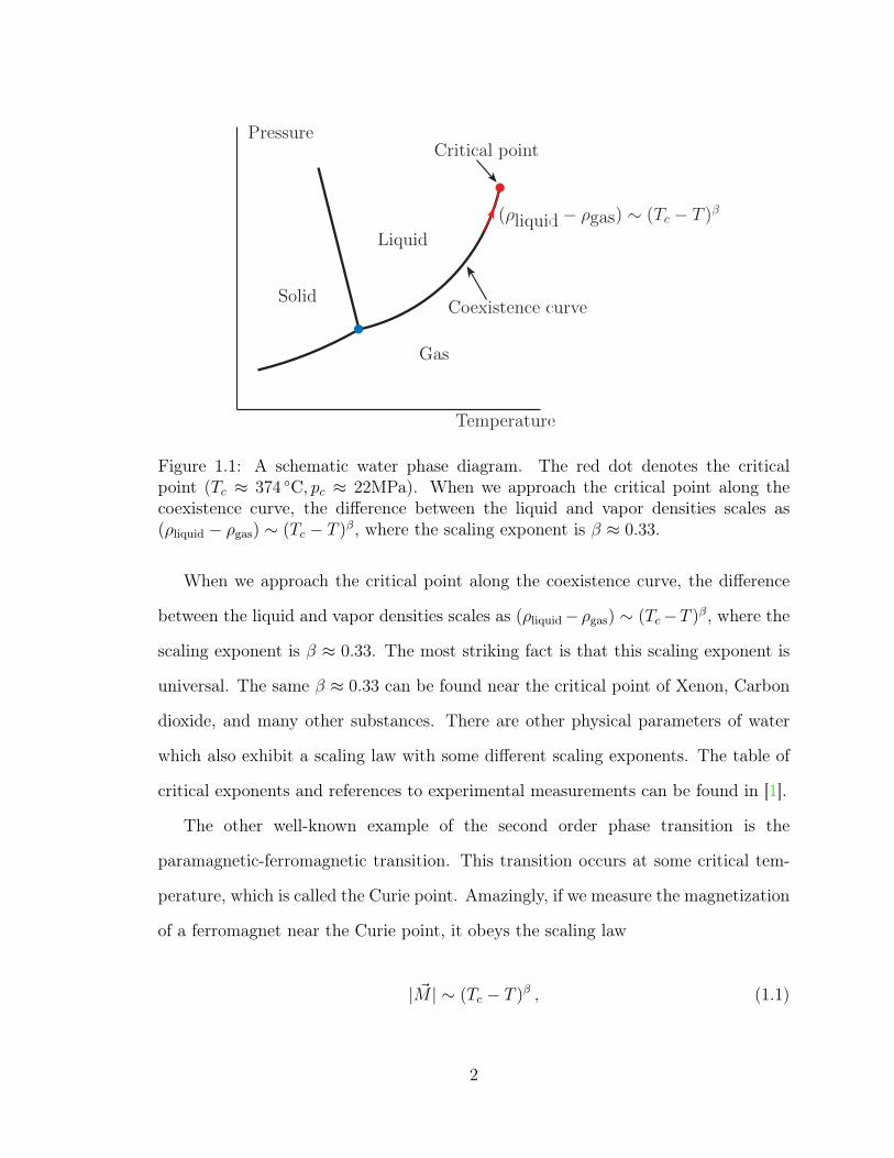
Figure 1.1: A schematic water phase diagram. The red dot denotes the criticalpoint (Tc ≈ 374 C, pc ≈ 22MPa). When we approach the critical point along thecoexistence curve, the difference between the liquid and vapor densities scales as(ρliquid − ρgas) ∼ (Tc − T )β, where the scaling exponent is β ≈ 0.33.

When we approach the critical point along the coexistence curve, the difference

between the liquid and vapor densities scales as (ρliquid−ρgas) ∼ (Tc−T )β, where the

scaling exponent is β ≈ 0.33. The most striking fact is that this scaling exponent is

universal. The same β ≈ 0.33 can be found near the critical point of Xenon, Carbon

dioxide, and many other substances. There are other physical parameters of water

which also exhibit a scaling law with some different scaling exponents. The table of

critical exponents and references to experimental measurements can be found in [1].

The other well-known example of the second order phase transition is the

paramagnetic-ferromagnetic transition. This transition occurs at some critical tem-

perature, which is called the Curie point. Amazingly, if we measure the magnetization

of a ferromagnet near the Curie point, it obeys the scaling law

| ~M | ∼ (Tc − T )β , (1.1)

2

where again β ≈ 0.33. This is a manifestation of the universality principle.

From a quantitative point of view, it is extremely difficult to obtain theoretical

predictions for the scaling exponents. This problem in Statistical Mechanics is closely

related to Quantum Field Theory, as we will see below. And this is still work in

progress, though much progress has been made in this direction. From a qualitative

point of view, second order phase transitions can be understood using the Landau

theory.

1.2 Landau theory

In 1937, in the seminal paper ”On the theory of phase transitions" [2], Landau for-

mulated a theory which gives a very good qualitative description of the second order

phase transition. Here we briefly repeat the main steps of this theory.

Consider the free energy F ( ~M, T ) of some magnetic material, where ~M is the

magnetization and T is the temperature. At high enough temperature, we expect

the magnetization to be very small, and therefore we can expand the free energy in a

Taylor series

F ( ~M, T ) = F0(T ) + a(T ) ~M2 + b(T )( ~M2)2 + . . . . (1.2)

The equilibrium magnetization can be found from the equation

∂F ( ~M, T )

∂ ~M= 0 . (1.3)

Obviously, when a(T ) > 0, the solution of this equation is ~M = 0. On the other

hand, if a(T ) < 0, the solution is | ~M | =√−a(T )2b(T )

. The Landau theory assumes that

near the critical point Tc, one can write a(T ) ≈ a0(T − Tc) and b(T ) ≈ b0. Thus it

3

gives for the magnetization

| ~M | ∼ (Tc − T )1/2, T < Tc and | ~M | = 0, T > Tc . (1.4)

So we see that though the Landau theory captures some basic properties of the second

order phase transition, it gives an incorrect prediction for the scaling exponent β,

which is not 0.5, but ≈ 0.33.

The Landau theory does not take into account fluctuations of the magnetization,

which become very important near the critical point. To improve this theory, one has

to assume that each configuration has its Boltzmann statistical weight

W ( ~M) = e− 1kBT

F ( ~M,T ). (1.5)

Also, we assume that the magnetization ~M is not a constant and may depend on

coordinates: ~M(x). Thus the free energy now can depend on derivatives of ~M(x) and

we have to consider the functional

F [ ~M(x), T ] =

∫d3x F ( ~M(x),∇ ~M(x), . . . , T ) . (1.6)

The Taylor expansion of the free energy now takes the form

F [ ~M(x), T ] =

∫d3x

(F0(T ) + a(T ) ~M2(x) + b(T )( ~M2(x))2 + c(T )(∇ ~M(x))2 + . . .

).

(1.7)

Finally the partition function, which is the sum over all different configurations with

the Boltzmann statistical weight, is

Z =

∫D ~M(x)e

− 1kBT

F [ ~M(x),T ]. (1.8)

4

After simple rescaling of the magnetization ~M(x) = z~φ(x) with a specially chosen

constant z, we arrive at the functional integral which describes the quantum field

theory of the scalar field ~φ

Z =

∫D~φ(x)e−S[~φ(x)] , (1.9)

with the Euclidean three-dimensional action

S[~φ(x)] =

∫d3x

(1

2(∇~φ)2 +

1

2m2~φ2 +

g

4!(~φ2)2 + . . .

). (1.10)

In the case of a magnet, ~φ is the vector with N = 3 components. For simplicity, we

can consider a theory where we have only one component:

S[φ(x)] =

∫d3x

(1

2(∇φ)2 +

1

2m2φ2 +

g

4!φ4 + . . .

). (1.11)

Theoretical analysis of this quantum field theory reveals the existence of the critical

point. And gives an extremely precise estimate for the critical exponents. In partic-

ular, it predicts β to be equal to 0.326 ± 0.003. The first quantitatively successful

result was achieved only in 1971 in the famous work of Wilson and Fisher [3]. In their

paper, they obtained β ≈ 0.306, which is already close to up-to-date results [4, 5].

1.3 Wilson’s approach to the Renormalization Group

In this section we briefly review Wilson’s approach to the Renormalization Group

(RG) [6] . We consider φ4 theory in general d dimensions. The action of the theory

reads

S[φ(x)] =

∫ddx

(1

2(∇φ)2 +

1

2m2φ2 +

g

4!φ4

). (1.12)

5

Assuming that the coupling constant g is small, we can expand the exponential of

the interaction tern in a Taylor series. Each order in perturbation theory can be

graphically represented by Feynman diagrams. If we try to compute these diagrams,

we find that they have divergences at short distances (UV divergences). Of course,

in real materials we have to cut off our integrals at the scale of a lattice size a, which

in the momentum representation, implies that all momenta are less than Λ ∼ 1/a.

Thus the Fourier transform of the field φ(x) is

φ(x) =

∫|k|<Λ

ddk

(2π)dφ(k)eikx . (1.13)

So the physically well-defined problem is to compute different correlation functions

in the theory with the cutoff Λ and the action (1.12):

〈φ(x1) . . . φ(xn)〉SΛ,Λ =1

Z

∫[Dφ]Λφ(x1) . . . φ(xn)e−SΛ[φ(x)] . (1.14)

Now we are going to perform Wilson’s renormalization procedure. Suppose now

we would like to integrate over all high-frequency fields from the frequency Λ1 to Λ,

where Λ1 < Λ. Namely, we can decompose the field φ(k) into a sum of two fields

φ(x) = φ1(x) + ϕ(x) , (1.15)

where φ1(x) and ϕ(x) are “slow” and “fast” fields defined through their Fourier trans-

forms

φ(x) =

∫|k|<Λ1

ddk

(2π)dφ(k)eikx, ϕ(x) =

∫Λ1<|k|<Λ

ddk

(2π)dφ(k)eikx . (1.16)

6

Next, we assume that the fields in the correlation function (1.14) have small Fourier

momenta, so we can replace these fields by the “slow” fields. Therefore we get

〈φ(x1) . . . φ(xn)〉SΛ,Λ =1

Z

∫[Dφ1]Λ1φ1(x1) . . . φ1(xn)

∫[Dϕ]e−SΛ[φ1+ϕ] . (1.17)

The new effective action SΛ1 is defined as

e−SΛ1[φ1] = c

∫[Dϕ]e−SΛ[φ1+ϕ] , (1.18)

where c is some unimportant constant, because we also have

Z =

∫[Dφ1]Λ1 [Dϕ]e−SΛ[φ1+ϕ] = c

∫[Dφ1]Λ1e

−SΛ1[φ1] = cZ1. (1.19)

Thus we finally obtain the following equality

〈φ(x1) . . . φ(xn)〉SΛ,Λ = 〈φ1(x1) . . . φ1(xn)〉SΛ1,Λ1 . (1.20)

In other words, it means that if we are interested only in low-momenta correlation

functions, the theory with the action SΛ and the cutoff Λ is equivalent to the theory

with the action SΛ1 and the cutoff Λ1.

What does the new action SΛ1 [φ1] look like? To compute it, one has to evaluate

a series of Feynman diagrams using the propagator of the “fast” field

〈ϕ(k)ϕ(−k)〉 =Θ(k)

k2 +m2, (1.21)

where Θ(k) = 1 if Λ1 < |k| < Λ and Θ(k) = 0 otherwise. It is not possible to

compute all Feynman diagrams, but analysis of the first few diagrams shows that the

new action SΛ1 [φ1] will contain infinitely many terms, which are powers of the field

7

φ1 and its derivatives:

SΛ1 [φ1] =

∫ddx

(1

2f0(∇φ1)2 +

1

2g2φ

21 +

∞∑n=2

g2n

(2n)!φ2n

1 (x) +∞∑n=1

f2n

(2n)!φ2n

1 (∇φ1)2 + . . .

).

(1.22)

Notice that in the action (1.11) we have dots, which represent higher terms in the

Taylor expansion of the functional (1.6). We omitted these higher terms in the action

(1.12), which has only a single φ4 interaction term. But after Wilson’s renormalization

procedure, we obtain the action (1.22), which again contains infinitely many terms.

The next step of Wilson’s procedure is to rescale coordinates x → x/l, where

l = Λ/Λ1 > 1. Namely, we make the variable transformation

φ1(x) = Z−1/2(l)φ′(x/l) , (1.23)

where Z(l) is some factor, which in principle can be arbitrary. This transformation

brings the cutoff parameter to its original value Λ and gives the new action

S ′Λ[φ′(x)] = SΛ1 [Z−1/2(l)φ′(x/l)] . (1.24)

Therefore, after Wilson’s full renormalization procedure, we obtain

〈φ(x1) . . . φ(xn)〉SΛ,Λ = Z−n/2(l)〈φ(x1/l) . . . φ(xn/l)〉S′Λ,Λ . (1.25)

Schematically, the RG transformation from the action SΛ to the action S ′Λ can be

written as

S ′ = RGt(S) , (1.26)

8

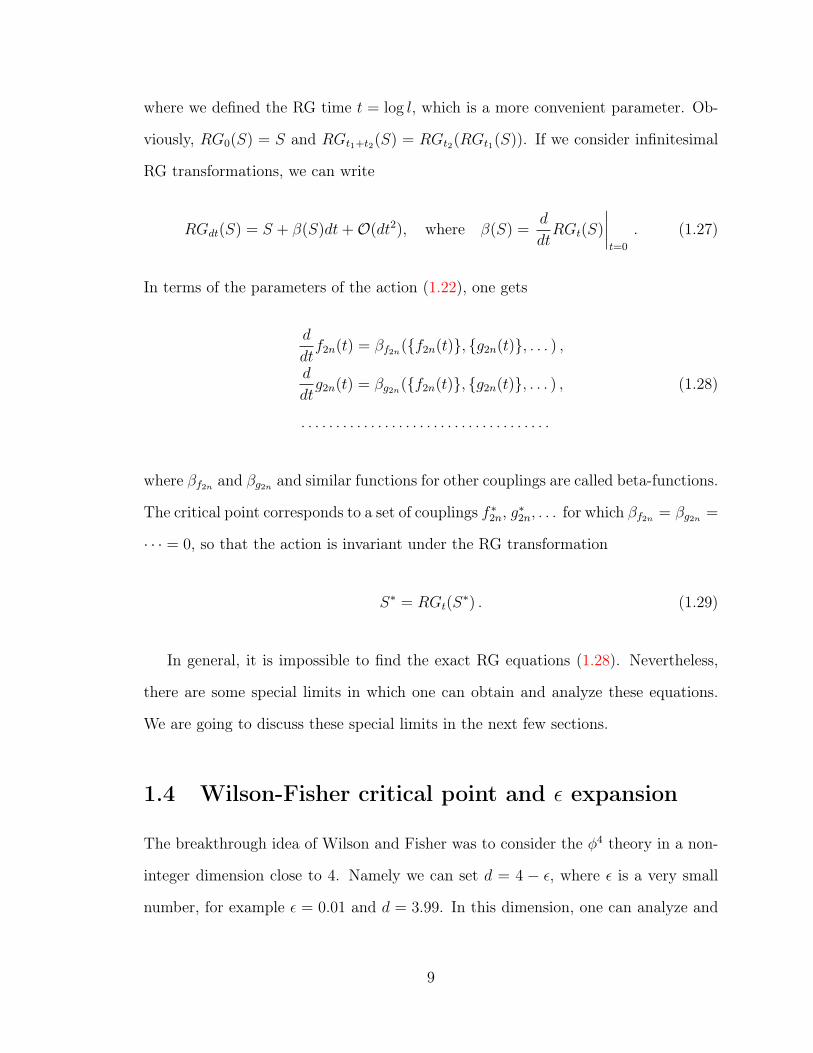
where we defined the RG time t = log l, which is a more convenient parameter. Ob-

viously, RG0(S) = S and RGt1+t2(S) = RGt2(RGt1(S)). If we consider infinitesimal

RG transformations, we can write

RGdt(S) = S + β(S)dt+O(dt2), where β(S) =d

dtRGt(S)

∣∣∣∣t=0

. (1.27)

In terms of the parameters of the action (1.22), one gets

d

dtf2n(t) = βf2n(f2n(t), g2n(t), . . . ) ,

d

dtg2n(t) = βg2n(f2n(t), g2n(t), . . . ) , (1.28)

. . . . . . . . . . . . . . . . . . . . . . . . . . . . . . . . . . . .

where βf2n and βg2n and similar functions for other couplings are called beta-functions.

The critical point corresponds to a set of couplings f ∗2n, g∗2n, . . . for which βf2n = βg2n =

· · · = 0, so that the action is invariant under the RG transformation

S∗ = RGt(S∗) . (1.29)

In general, it is impossible to find the exact RG equations (1.28). Nevertheless,

there are some special limits in which one can obtain and analyze these equations.

We are going to discuss these special limits in the next few sections.

1.4 Wilson-Fisher critical point and ε expansion

The breakthrough idea of Wilson and Fisher was to consider the φ4 theory in a non-

integer dimension close to 4. Namely we can set d = 4 − ε, where ε is a very small

number, for example ε = 0.01 and d = 3.99. In this dimension, one can analyze and

9

solve the equations (1.28). Namely, the one-loop computation gives

d

dtg2 =

(2− g4

(4π)2+O(g2

4))g2 ,

d

dtg4 = εg4 −

3g24

(4π)2+O(g3

4) ,

d

dtg6 = (−2 + 2ε+O(g4))g6 , (1.30)

. . . . . . . . . . . . . . . . . . . . . . . . . . . . . .

Equations for the other couplings will have a similar form. Amazingly, these equations

have the fixed-point solution

g∗2 = 0, g∗4 =(4π)2

3ε+O(ε2), g∗6 = 0, . . . (1.31)

This one-loop approximation is legitimate because ε is a small parameter and includ-

ing higher-loop Feynman diagrams would give corrections to g∗4 of order ε2 and higher.

This critical point is called the Wilson-Fisher (WF) fixed point.

Now if we start with the critical point action S∗ and perturb it by operators φ

and φ2 1

S = S∗ + δg

∫ddxφ(x) + δm2

∫ddxφ2(x) (1.32)

we can compute their RG flow and get

d

dt〈φ〉 = ∆φ〈φ〉 ,

d

dtm2 = ∆m2m2 , (1.33)

1Here we use notation δm2 instead of δg2.

10

where the anomalous dimensions are

∆φ =(

1− ε

2+

(g∗4)2

12(4π)4+O(ε3)

), ∆m2 =

(2− g∗4

(4π)2+O(ε2)

). (1.34)

The equations (1.33) have a simple solution

〈φ(t)〉 = 〈φ0〉e∆φt, m2(t) = δm2e∆m2 t . (1.35)

Therefore we finally obtain

〈φ(t)〉 ∼ (m2(t))∆φ

∆m2 . (1.36)

In fact 〈φ〉 is proportional to the magnetization, while m2 is proportional to the

deviation of the temperature from the critical value. Therefore, the formula (1.36)

gives

| ~M | ∼ (Tc − T )β, β =∆φ

∆m2

=1− ε

2+ ε2

108

2− ε3

. (1.37)

Now the magic trick is to set ε = 1 and obtain the result for the three-dimensional

theory: β = 0.306. The trick works because the ε- expansion converges very fast and

higher powers of ε don’t change the result considerably.

1.5 Large N approximation

The idea of the large N approximation is to replace a single scalar field φ by a vector

φi, where i = 1, . . . , N . So the action for the vector field φi takes the form

S[φi(x)] =

∫ddx

(1

2(∇φi)2 +

1

2m2φiφi +

g

4(φiφi)2

). (1.38)

11

We notice that this action is invariant under global O(N) transformations of the

vector field φi →M ijφj, where M is an orthogonal matrix.

When N is large, it is possible to develop an expansion in 1/N . At leading order,

one needs to sum only diagrams which look like a chain of bubbles, see figure 1.2.

Figure 1.2: An example of a Feynman diagrams dominating at the large N limit.

Using this one can compute anomalous dimensions of the operators φi and φiφi

as series in 1/N . In fact, it is possible to obtain the coefficients of this series for

arbitrary dimension d. The results are

∆φ =d− 2

2+

2 sin(πd2

)Γ(d− 2)

πΓ(d2− 2)

Γ(d2

+ 1) 1

N+O(1/N2) ,

∆φ2 = 2 +4 sin

(πd2

)Γ(d)

πΓ(d2− 1)

Γ(d2

+ 1) 1

N+O(1/N2) . (1.39)

In the case of d = 3, these formulas give

∆φ =1

2+

4

3π2

1

N+O(1/N2) ,

∆φ2 = 2− 32

3π2

1

N+O(1/N2) . (1.40)

One also finds for the scaling exponent β:

β =∆φ

3−∆φ2

=1 + 8

3π21N

2(1 + 323π2

1N

), (1.41)

where we used that ∆m2 = d − ∆φ2 . Quite surprisingly, setting N = 1, we obtain

β = 0.305, which is not far from the correct result. In this case we should not expect

12

that setting N = 1 gives a precise result because the 1/N series converges slowly and

subleading 1/N corrections become small only for big enough N .

We also note that today the most accurate method of finding anomalous di-

mensions of the O(N) model for arbitrary N belongs to the Bootstrap approach

[7, 8, 9, 10, 4]. By imposing crossing relations on the four-point functions of fields φ

and φ2 it is possible to determine an allowed region for ∆φ and ∆φ2 . The accuracy

of this method is phenomenal and is equal to five digits after the decimal point! The

bootstrap results are ∆φ = 0.51816 and ∆φ2 = 1.41267, which gives β = 0.32643.

1.6 Conformal Quantum Electrodynamics

The four-dimensional Quantum Electrodynamics coupled to Nf Dirac fermions is an

original model of Quantum Field Theory; its predictions have been verified experimen-

tally with high accuracy. If the fermions are massless, then the theory is conformally

invariant for zero charge e, but the interaction effects are well known to break the

conformal invariance. They produce a positive β function for e, which means that

the theory becomes free at long distances.

The physics of QED is different in d 6= 4. Then the free Maxwell action 14FµνF

µν is

not conformally invariant [11], but the one loop fermion vacuum polarization diagram

induces a scale invariant quadratic term proportional to

Fµν(−∇2)d2−2F µν , (1.42)

which is in general non-local. For d < 4 this term dominates at long distances, and

well-known examples of such “induced QED” are the Schwinger model [12] in d = 2

and the conformal phase of QED3 [13, 14]. In d = 4− ε the conformal QEDd theory

13

may be studied using the ε expansion, because the β function

β = − ε2e+

4Nf

3

e3

(4π)2+O(e5) (1.43)

has a weakly coupled IR fixed point at e2∗ = 6επ2/Nf +O(ε2) [15]. The ε expansion

of various operator dimensions in QEDd was introduced in [16, 17].

Among the important physical applications of the conformal QED is the theory in

d = 3 coupled to massless Dirac fermions and/or complex scalars. An early motivation

to study QED3 came from work on the high temperature behavior of four-dimensional

gauge theory [13]. More recently, its various applications to condensed matter physics

have been explored as well (see, for example, [18, 19, 20]). Work on QED3 has

uncovered a variety of interesting phenomena, which include chiral symmetry breaking

and interacting conformal field theory [21, 22, 14]. Both of these phases of the theory

are consistent with the Vafa-Witten theorem [23], which requires the presence of

massless modes for Nf > 3. Yet, some questions remain about the infrared behavior

of the theory.

1.7 Tensor models

In the section (1.5) we replaced a scalar field φ by a vector φi, where i = 1, . . . , N .

Taking the large N limit we saw that only a special set of diagrams contributing.

It is possible to compute all the diagrams in this set and obtain results as a series

in 1/N . The next logical step is to promote a vector field φi to a matrix φij with

i, j = 1, . . . , N . The action for such a matrix can take the form

S[φij(x)] =

∫ddx

(1

2(∇φij)2 +

1

2m2φijφij +

g1

4(φijφij)2 +

g2

4(φi1j1φi1j2φi2j1φi2j2)

).

(1.44)

14

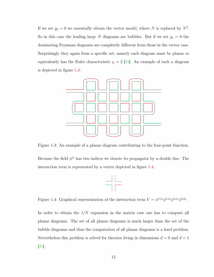
If we set g2 = 0 we essentially obtain the vector model, where N is replaced by N2.

So in this case the leading large N diagrams are bubbles. But if we set g1 = 0 the

dominating Feynman diagrams are completely different from those in the vector case.

Surprisingly they again form a specific set, namely each diagram must be planar or

equivalently has the Euler characteristic χ = 2 [24]. An example of such a diagram

is depicted in figure 1.3.

Figure 1.3: An example of a planar diagram contributing to the four-point function.

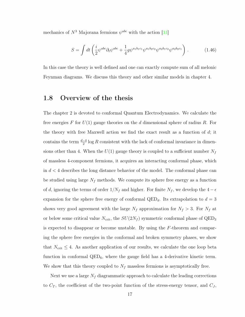
Because the field φij has two indices we denote its propagator by a double line. The

interaction term is represented by a vertex depicted in figure 1.4.

Figure 1.4: Graphical representation of the interaction term V = φi1j1φi1j2φi2j1φi2j2 .

In order to obtain the 1/N expansion in the matrix case one has to compute all

planar diagrams. The set of all planar diagrams is much larger than the set of the

bubble diagrams and thus the computation of all planar diagrams is a hard problem.

Nevertheless this problem is solved for theories living in dimensions d = 0 and d = 1

[25].

15

The next obvious step in our discussion is to add one more index to the matrix

φij promoting it to a tensor φijk, where i, j, k = 1, . . . , N . In this case one can find a

new fascinating large N limit for the interaction [26, 27, 28]

V = φi1j1k1φi1j2k2φi2j1k2φi2j2k1 . (1.45)

Its graphical representation is depicted in figure 1.5.

Figure 1.5: Graphical representation of the interaction term V =φi1j1k1φi1j2k2φi2j1k2φi2j2k1 .

In this case the leading large N limit is dominated by a specific set of diagrams,

which are called melonic diagrams [29, 30]. An example of a melonic diagram con-

tributing to the four-point function is depicted in figure 1.6. Here we denote each

propagator by a single line. One can also represent diagrams in stranded way, where

propagators are triple lines and vertices look like in the matrix case, but with two

additional crossing lines.

Figure 1.6: An example of a melonic diagram contributing to the four-point function.

Unfortunately the interaction (1.45) for bosonic fields is not bounded from below.

This leads to instability of the theory. Nevertheless one can consider a quantum16

mechanics of N3 Majorana fermions ψabc with the action [31]

S =

∫dt

(i

2ψabc∂tψ

abc +1

4gψa1b1c1ψa1b2c2ψa2b1c2ψa2b2c1

). (1.46)

In this case the theory is well defined and one can exactly compute sum of all melonic

Feynman diagrams. We discuss this theory and other similar models in chapter 4.

1.8 Overview of the thesis

The chapter 2 is devoted to conformal Quantum Electrodynamics. We calculate the

free energies F for U(1) gauge theories on the d dimensional sphere of radius R. For

the theory with free Maxwell action we find the exact result as a function of d; it

contains the term d−42

logR consistent with the lack of conformal invariance in dimen-

sions other than 4. When the U(1) gauge theory is coupled to a sufficient number Nf

of massless 4-component fermions, it acquires an interacting conformal phase, which

in d < 4 describes the long distance behavior of the model. The conformal phase can

be studied using large Nf methods. We compute its sphere free energy as a function

of d, ignoring the terms of order 1/Nf and higher. For finite Nf , we develop the 4− ε

expansion for the sphere free energy of conformal QEDd. Its extrapolation to d = 3

shows very good agreement with the large Nf approximation for Nf > 3. For Nf at

or below some critical value Ncrit, the SU(2Nf ) symmetric conformal phase of QED3

is expected to disappear or become unstable. By using the F -theorem and compar-

ing the sphere free energies in the conformal and broken symmetry phases, we show

that Ncrit ≤ 4. As another application of our results, we calculate the one loop beta

function in conformal QED6, where the gauge field has a 4-derivative kinetic term.

We show that this theory coupled to Nf massless fermions is asymptotically free.

Next we use a large Nf diagrammatic approach to calculate the leading corrections

to CT , the coefficient of the two-point function of the stress-energy tensor, and CJ ,

17

the coefficient of the two-point function of the global symmetry current. We present

explicit formulae as a function of d and check them versus the expectations in 2 and 4−

ε dimensions. Using our results in higher even dimensions we find a concise formula for

CT of the conformal Maxwell theory with higher derivative action Fµν(−∇2)d2−2F µν .

In d = 3, QED has a topological symmetry current, and we calculate the correction

to its two-point function coefficient, CtopJ . We also show that some RG flows involving

QED in d = 3 obey CUVT > CIR

T and discuss possible implications of this inequality

for the symmetry breaking at small values of N .

In chapter 3 we study vacuum stability in 1 + 1 dimensional Conformal Field

Theories with external background fields. We show that the vacuum decay rate is

given by a non-local two-form. This two-form is a boundary term that must be added

to the effective in/out Lagrangian. The two-form is expressed in terms of a Riemann-

Hilbert decomposition for background gauge fields, and its novel “functional” version

in the gravitational case.

In chapter 4 we study the tensor models. Certain tensor models with rank-3 ten-

sor degrees of freedom possess a novel large N limit, where g2N3 is held fixed. In this

limit the perturbative expansion in the quartic coupling constant, g, is dominated by

a special class of “melon" diagrams. We study “uncolored" models of this type, which

contain a single copy of real rank-3 tensor. Its three indices are distinguishable; there-

fore, the models possess O(N)3 symmetry with the tensor field transforming in the

tri-fundamental representation. Such uncolored models also possess the large N limit

dominated by the melon diagrams. The quantum mechanics of a real anti-commuting

tensor therefore has a similar large N limit to the Sachdev-Ye-Kitaev (SYK) model,

but does not require disorder. Gauging the O(N)3 symmetry in our quantum mechan-

ical model removes the non-singlet states; therefore, one can search for its well-defined

gravity dual. We point out, that the model possesses a vast number of gauge-invariant

operators involving higher powers of the tensor field, suggesting that the complete

18

gravity dual will be intricate. We also discuss the quantum mechanics of a complex

3-index anti-commuting tensor, which has U(N)2 × O(N) symmetry and argue that

it is equivalent in the large N limit to a version of SYK model with complex fermions.

Finally, we study the spectrum of the large N quantum field theory of bosonic

rank-3 tensors, whose quartic interactions are such that the perturbative expansion

is dominated by the melonic diagrams. We use the Schwinger-Dyson equations to

determine the scaling dimensions of the bilinear operators of arbitrary spin. Using

the fact that the theory is renormalizable in d = 4, we compare some of these results

with the 4 − ε expansion, finding perfect agreement. This helps elucidate why the

dimension of operator φabcφabc is complex for d < 4: the largeN fixed point in d = 4−ε

has complex values of the couplings for some of the O(N)3 invariant operators. We

show that a similar phenomenon holds in the O(N)2 symmetric theory of a matrix

field φab, where the double-trace operator has a complex coupling in 4− ε dimensions.

We also study the spectra of bosonic theories of rank q−1 tensors with φq interactions.

In dimensions d > 1.93 there is a critical value of q, above which we have not found

any complex scaling dimensions. The critical value is a decreasing function of d, and

it becomes 6 in d ≈ 2.97. This raises a possibility that the large N theory of rank-

5 tensors with sextic potential has an IR fixed point which is free of perturbative

instabilities for 2.97 < d < 3.

19

Chapter 2

Conformal QED

This chapter is an edited version of ref. [32] and [33] written in collaboration with

Simone Giombi and Igor Klebanov. The first part of the chapter is devoted to com-

putation of the sphere free energy in the conformal QED in d dimensions. In the

second part we compute CT and CJ in the conformal QED in d dimensions.

2.1 Introduction and Summary

2.1.1 Conformal Quantum Electrodynamics

In this chapter we study infrared behavior of QED using the relatively new tools

provided by the F -theorem [34, 35, 36, 37]. Our analysis is similar in spirit to that

of [38, 39], although some of our reasoning is different. We will work with the U(1)

gauge theory coupled to Nf massless 4-component Dirac fermions ψj. The lagrangian

of this theory has SU(2Nf ) global symmetry, which is often referred to as the “chiral

symmetry.” In QED3 the fine structure constant α = e2

4πhas dimension of mass; this

makes the theory super-renormalizable. At short distances we find a weakly interact-

ing theory of massless fermions and photons, where the field strength Fµν has scaling

dimension 3/2. The short distance limit of QED3 is scale invariant, but not confor-

20

mal. This is because the free Maxwell action 14FµνF

µν is not conformally invariant in

three dimensions [11]. The lack of conformal invariance of the free Maxwell theory

translates into the fact that its three-sphere free energy F depends logarithmically on

the sphere radius R [40]. In section 2.2 we will generalize this result to free Maxwell

theory on Sd and show that its free energy contains the term d−42

logR. We will refer

to the short distance limit of QED3 as the UV theory. The fact that its F value, FUV,

diverges is important for consistency of the RG flows with the F -theorem.

As QED3 flows to longer distances, the effective interaction strength grows and

various interesting phenomena become possible. The one loop fermion vacuum polar-

ization diagram induces a non-local quadratic term (1.42) for Aµ, which dominates

in the IR over the Maxwell term [13]. Due to this effect, the theory flows to an

interacting conformal field theory in the large Nf limit where e2Nf is held fixed. In

the CFT the scaling dimension of Fµν is 2. The scaling dimensions of other operators

can be calculated as series in 1/Nf (see, for example, [41, 42, 43]).

A different possibility is the spontaneous breaking of the SU(2Nf ) global symme-

try due to generation of vacuum expectation value of the operator∑Nf

j=1 ψjψj (it is

written using the 4-d notation for spinors ψi and gamma-matrices). This operator

preserves the 3-d parity and time reversal symmetries, but it breaks the global sym-

metry to SU(Nf ) × SU(Nf ) × U(1). This mechanism was proposed in [21], where

it was argued using Schwinger-Dyson equations to be possible for any Nf ; however,

for large Nf the scale of the VEV becomes exponentially small compared to α. Sub-

sequently, modified treatments of the Schwinger-Dyson equations [14] suggested that

the chiral symmetry breaking is possible only for Nf ≤ Ncrit. The estimates of Ncrit

typically range between 2 and 10 [44, 45, 46, 17].

It is widely believed that the QED3 must be in the conformal phase for Nf >

Ncrit, but a nearly marginal operator may appear in the spectrum of the CFT as

Nf is reduced towards Ncrit. This operator must respect the SU(2Nf ) and parity

21

symmetries of the theory, and natural candidates are the operators quartic in the

fermion fields [17] (see also [43, 46]).1

When the quartic operator is slightly irrelevant, it should give rise to a nearby UV

fixed point; there is a standard argument for this using conformal perturbation theory,

which we present in section 2.6. We will call this additional fixed point QED∗3. For

Nf = Ncrit it merges with QED3, and for Nf < Ncrit both fixed points may become

complex [44, 48, 49, 46]. In this “merger and annihilation of fixed points" scenario,

for Nf < Ncrit the UV theory flows directly to the broken symmetry phase.

Alternatively, both fixed points may stay real and go through each other. Then the

QED3 fixed point continues to exist even after the appearance of a relevant operator;

this relevant operator may create flow from QED3 to the broken symmetry phase.

If so, the edge of the conformal window may be associated with the dimension of

some operator in QED3 becoming so small that it violates the unitarity bound. This

would be analogous to what happens at the lower edge of the conformal window in

the N = 1 supersymmetric gauge theory [50].

2.1.2 Sphere free energy and the F -theorem in QED

We will attempt to shed new light on the transition from the conformal to the sym-

metry breaking behavior by using the F -theorem and performing more precise calcu-

lations of F . Here F = − logZS3 is the 3-sphere free energy [34, 35] or, equivalently,

the long-range Entanglement Entropy across a circle [36, 37]. The theorem states that

for Renormalization Group (RG) flow from fixed point 1 to fixed point 2, F1 > F2.

A proof of this inequality has been found using properties of the Renormalized En-

tanglement Entropy in relativistic field theories [51] (see also [52]).1 In the compact theory, monopole operators may also become relevant as one lowers Nf [47];

however, these operators transform in non-trivial representations of the SU(2Nf ) flavor symme-try, and so they are not expected to be generated along the RG flow if the UV theory has exactSU(2Nf ) symmetry. Monopoles may still condense, i.e. they may acquire expectation values in thespontaneously broken phase.

22

In order to apply the F -theorem to RG flows among different phases of QED3, it

is important to know their F -values. This is especially challenging for the interacting

CFT phase of the theory. In [40] this calculation was performed using the 1/Nf

expansion with the result

Fconf = Nf

(log(2)

2+

3ζ(3)

4π2

)+

1

2log

(πNf

4

)+O(

1

Nf

) . (2.1)

The first term on the RHS is the F -value of Nf free Dirac fermions, NfFfree−ferm.

Even though Fconf − NfFfree−ferm grows without bound for large Nf , the F -theorem

inequality FUV > Fconf is satisfied. This is because FUV is infinite due to the diver-

gent contribution of the free Maxwell theory. In section 2.3 we review the large N

description of conformal QED and generalize the result (2.1) by computing Fconf as

a function of d.

Since we will be quite interested in Fconf for small Nf , in this paper we will apply

a different approximation method [53, 54]. This method consists of developing the ε

expansion of F = − sin(πd/2)FSd for d = 4−ε. It relies on the perturbative renormal-

ization of the field theory on the sphere S4−ε and requires inclusion of counter terms

that involve the curvature tensor [55, 56, 57, 58, 59]. Applications of this method

to the Wilson-Fisher O(N) symmetric CFTs have produced high-quality estimates

of FO(N) in d = 3; they are found to be only 2 − 3% below the F values for the

corresponding free UV fixed points of these theories [53, 54].

In this chapter, we will perform a similar ε expansion for F of the conformal QED,

building on earlier work which developed the perturbative renormalization of QED

on S4−ε [60, 61, 59, 62, 63]. This calculation is presented in section 2.5, and our main

23

result is

Fconf = Nf Ffree-ferm −1

2sin(

πd

2) log(

Nf

ε)

+31π

90− 1.2597ε− 0.6493ε2 + 0.8429ε3 +

0.4418ε2

Nf

− 0.6203ε3

Nf

− 0.5522ε3

N2f

+O(ε4) .

(2.2)

Extrapolating this to d = 3 using Padé approximants produces results very close to

the large Nf formula (2.1) already for Nf > 3, see figure 2.4.

Applying the F -theorem, we find that RG flow from the conformal to the broken

symmetry phase is impossible when Fconf < FSB. This puts an upper bound on the

value Ncrit where the conformal phase can become unstable [38]. Using our resummed

ε expansion results for Fconf , we find that the value of Nf where Fconf = FSB rather

robustly lies between 4 and 5, and our best estimate is Nf ≈ 4.4. If we restrict to

integer values of Nf , this means that for Nf ≥ 5 the QED3 theory must be in the

SU(2Nf ) symmetric conformal phase. Therefore, our results give the upper bound

Ncrit ≤ 4. The same upper bound is obtained if we use the large Nf approximation

(2.1) to Fconf , which was derived in [40]. The results obtained using the ε expansion

of quartic operator dimensions [17], as well as computations in lattice gauge theory

[64, 65], are consistent with our upper bound.

2.1.3 Two point function of the stree-energy tensor in QED

The other important observables in Conformal Field Theory (CFT) is CT , the coef-

ficient of the two-point function of the stress-energy tensor Tµν , defined via [66]

〈Tµν(x1)Tλρ(x2)〉 = CTIµν,λρ(x12)

(x212)d

, (2.3)

24

where

Iµ ν,λρ(x) ≡ 1

2(Iµλ(x)Iνρ(x) + Iµρ(x)Iνλ(x))− 1

dδµνδλρ ,

Iµν(x) ≡ δµν − 2xµxνx2

. (2.4)

If the CFT has a global symmetry generated by conserved currents Jaµ , then another

interesting observable is CJ , the coefficient of their two-point functions:

〈Jaµ(x1)J bν(x2)〉 = CJIµν(x12)

(x212)d−1

δab . (2.5)

In CFTs with a large number of degrees of freedom, N , these observables typically

admit 1/N expansions of the form

CJ = CJ0

(1 +

CJ1

N+CJ2

N2+O(1/N3)

),

CT = CT0

(1 +

CT1

N+CT2

N2+O(1/N3)

). (2.6)

The values of CJ1 and CT1 have been calculated in a variety of models. Petkou [67]

has used large N methods and operator products expansions to calculate them as a

function of d in the scalar O(N) model. Very recently, these results were reproduced

using the large N diagrammatic approach in [68], where the same technique was also

used to calculate CJ1 and CT1 as a function of d in the conformal Gross-Neveu model.

An important feature of the diagrammatic approach, which was uncovered in [68],

is the necessity, in the commonly used regularization scheme [69, 70, 71, 72, 73], of

a divergent multiplicative “renormalization" ZT for the stress-energy tensor. This

factor is required by the conformal Ward identities in the regularized theory.

In this chapter we extend the methods of [68] to calculate CJ1(d) and CT1(d) in

the conformal QED in d dimensions. This theory, which is reviewed in section 2.3,

may be thought of as the Maxwell field coupled to Nf massless 4-component Dirac

25

fermions continued from 4 dimensions to a more general dimension d. The large N

expansion in this model runs in powers of the total number of fermionic components,

which is N = 4Nf . In the physically interesting dimension d = 3, this corresponds to

an even number 2Nf of two-component Dirac fermions.

Our main results are

CJ1(d) = ηm1

(3d(d− 2)

8(d− 1)Θ(d) +

d− 2

d

), (2.7)

CT1(d) = ηm1

(3d(d− 2)

8(d− 1)Θ(d) +

d(d− 2)

(d− 1)(d+ 2)Ψ(d)− (d− 2)(3d2 + 3d− 8)

2(d− 1)2d(d+ 2)

),

(2.8)

Θ(d) ≡ ψ′(d/2)− ψ′(1) , Ψ(d) ≡ ψ(d− 1) + ψ(2− d/2)− ψ(1)− ψ(d/2− 1) ,

where ψ(x) = Γ′(x)/Γ(x). Here ηm1(d) encodes the electron mass anomalous dimen-

sion; it is [74]2

ηm1(d) = − 2(d− 1)Γ(d)

Γ(d2)2Γ(d

2+ 1)Γ(2− d

2). (2.9)

In the physically interesting case of d = 3 we find

CJ1(3) =736

9π2− 8 ≈ 0.285821 ,

CT1(3) =4192

45π2− 8 ≈ 1.43863 . (2.10)

A nontrivial check of our results (2.7) and (2.8) comes from comparing them with

the known exact values in d = 2 and the 4 − ε expansions, see sections 2.7 and 2.9.

Had we not included ZT , there would be no agreement with the 4 − ε expansion.

In higher even d, the conformal QED reduces to a free theory of N fermions and a2We define the anomalous dimension of the electron mass operator Om = ψψ as ∆Om = d−1+ηm,

where ηm = ηm1/N +O(1/N2).

26

conformal higher-derivative Maxwell theory with the action (see e.g. [33])

Fµν(−∇2)d2−2F µν . (2.11)

Using the value of CT1 in general even dimensions, we extract the CT of this conformal

Maxwell theory

Cconf. MaxwellT |even d = (−1)

d2d

S2d

(d

d2− 1

), (2.12)

where Sd = 2πd/2

Γ(d/2).

In d = 3 the QED has a special “topological" U(1) symmetry current jtop = 12π∗F .

In section 2.8 we calculate its two-point function to order 1/N2, and obtain the

associated CtopJ coefficient, in the normalization (2.5), to be

CtopJ =

16

π4N

(1 +

1

N

(8− 736

9π2

)+O(1/N2)

), (2.13)

where N = 4Nf is twice the number of two-components Dirac fermions. The leading

order term is in agreement with [75, 76].

As we already mentioned above the QED3 Lagrangian also has an enhanced

SU(2Nf ) global symmetry, and for small Nf this symmetry may be broken spon-

taneously to SU(Nf )×SU(Nf )×U(1). In section 2.10 we present a new estimate for

the critical value of Nf above which the symmetry breaking cannot occur by using

the RG inequality CUVT > CIR

T . It implies that the chiral symmetry cannot be broken

for Nf > 1 +√

2. The status of this conclusion is uncertain, since there are known

violations of the inequality in some supersymmetric RG flows [77]. Nevertheless, it is

interesting that the critical value of Nf it yields is close to other available estimates

[44, 45, 46, 17] and our estimate from the F -theorem and is consistent with the results

available from lattice gauge theory [64, 65].

27

2.2 Sphere free energy of Maxwell theory on Sd

The action for Maxwell theory on a curved manifold is

S =

∫ddx√g

1

4e2FµνF

µν =1

2e2

∫ddx√gAν

(−δµν∇2 +Rµ

ν +∇ν∇µ)Aµ , (2.14)

where we have used Fµν = ∇µAν − ∇νAµ and [∇µ,∇ν ]Aµ = RµνAµ. On a round Sd

of radius R, we have Rµν = d−1

R2 δµν and so the action is

S =

∫Sdddx√g

1

2e2Aν(δµν (−∇2 +

d− 1

R2) +∇ν∇µ

)Aµ . (2.15)

The partition function is given by

Z =1

vol(G)

∫DAe−S(A) , (2.16)

where G is the volume of the group of gauge transformations. One way to proceed is

to split the gauge field into transverse and pure gauge part3

Aµ = Bµ + ∂µφ , ∇µBµ = 0 . (2.17)

Following [40], we have

DA = DBD(dφ) = DBD′φ√

det′(−∇2)

vol(G) = 2π√

vol(Sd)

∫D′φ , vol(Sd) =

2πd+1

2

Γ(d+1

2

)Rd ≡ ΩdRd ,

(2.18)

3Equivalently, one can use Feynman gauge by adding a gauge fixing term Lfix = 12 (∇µAµ)2.

This gauge is more convenient for perturbative calculations when interactions with matter fields areincluded, and we will use it in Section 2.5.

28

where prime means that the constant mode is not included. Then, the partition

function can be written as

Z =

√det′(−∇2)

2π√

vol(Sd)

∫DBe−

∫Sd

ddx√g 1

2e2Bµ(−∇2+ d−1

R2 )Bµ

=1

2π√

vol(Sd)

√det′(−∇2)√

detT (−∇2+(d−1)/R2

2πe2), (2.19)

where the subscript ‘T ’ indicates that the determinant is taken on the space of trans-

verse vector fields.

The eigenvalues of the sphere Laplacian −∇2 acting on a transverse vector and

corresponding degeneracies are known to be (see e.g. [78, 79])

λ(1)` =

1

R2(`(`+d−1)−1) , g

(1)` =

`(`+ d− 1)(2`+ d− 1)Γ (`+ d− 2)

Γ (`+ 2) Γ (d− 1), ` ≥ 1 .

(2.20)

For a scalar field, one has

λ(0)` =

1

R2`(`+ d− 1) , g

(0)` =

(2`+ d− 1)Γ (`+ d− 1)

Γ (`+ 1) Γ (d), ` ≥ 0 . (2.21)

In the case of the scalar field, ` = 0 corresponds to the constant mode which is to be

excluded in our case. Using these results, the free energy of Maxwell theory on Sd,

FMaxwell = − logZ, can be written as

FMaxwell =1

2

∞∑`=1

g(1)` log(

(`+ 1)(`+ d− 2)

2πe2R2)

− 1

2

∞∑`=1

g(0)` log(

`(`+ d− 1)

R2) + log(2π

√vol(Sd)) . (2.22)

29

In dimensional regularization, the following results for the sum over vector and scalar

degeneracies hold

∞∑`=1

g(1)` = 1,

∞∑`=0

g(0)` = 0 , →

∞∑`=1

g(0)` = −1 . (2.23)

These can be obtained for example by evaluating the sums for sufficiently negative d

where they converge, and analytically continuing to positive values of d. Using these

regularized identities, one can readily extract the radius dependence of the Maxwell

free energy (2.22) to be

FMaxwell = −1

2log(e2R4−d) + F

(0)Max.(d) , (2.24)

where F (0)Max.(d) is a radius independent function of d (with simple poles at even d).

In particular, we see that FMaxwell → +∞ in the short distance limit for d < 4. The

function F (0)Max.(d) can be evaluated in continuous d by computing the non-trivial sums

in (2.22), as we explain below.

We first find it convenient to rewrite the free energy in the following way

FMaxwell = Fvector − 2Fmin−sc + Fmeasure , (2.25)

where we have defined

Fvector =1

2

∞∑`=1

g(1)` log(

(`+ 1)(`+ d− 2)

2πe2R2) +

1

2

∞∑`=1

g(0)` log(

`(`+ d− 1)

R2) ,

Fmin−sc =1

2log det′(−∇2) =

1

2

∞∑`=1

g(0)` log(

`(`+ d− 1)

R2) ,

Fmeasure = log(2π√

vol(Sd)) .

(2.26)

The grouping of terms in (2.25) is essentially equivalent to doing the calculation in

Feynman gauge, where one has an unconstrained vector and a complex minimally

30

coupled scalar ghost. To proceed, we use the identity

log(y) =

∫ ∞0

dt

t

(e−t − e−yt

). (2.27)

Then, using the dimensionally regularized identities (2.23), one can rewrite the vector

contribution as

Fvector =− 1

2

∫ ∞0

dt

t

[∞∑`=1

g(1)` (e−(`+1)t + e−(`+d−2)t) + g

(0)` (e−`t + e−(`+d−1)t)

]

− 1

2log(2πe2) . (2.28)

Note that the radius dependence in Fvector, and the terms proportional to e−t, have

dropped out due to (2.23). The sum over ` can now be evaluated analytically, leading

to elementary functions of e−t. To perform the t-integral, it is convenient to use the

identity1

t=

1

1− e−t∫ 1

0

due−ut . (2.29)

This allows for an analytical evaluation of the t integral, and after some algebra and

using gamma function identities such as Γ(x)Γ(1 − x) = π csc(πx), we arrive at the

result

Fvector =

∫ 1

0

du

[(d2 + 1− 3d(1 + u) + 2u(u+ 2)) sin(

π

2(d− 2u))

× Γ (d− 2− u) Γ (1 + u)

2 sin(πd2

)Γ (d)− d− 2

(d− 2)2 − u2

]− 1

2log(2πe2) . (2.30)

To evaluate the ghost contribution Fmin−sc by similar methods, we can introduce a

small regulator to deal with the zero mode, so that we can extend the sum over all

modes and make use of (2.23)

Fmin−sc = limδ→0

[−1

2

∫ ∞0

dt

t

∞∑`=0

g(0)` (e−(`+δ)t + e−(`+d−1)t)− 1

2log(

δ(d− 1)

R2)

]. (2.31)

31

Performing first the sum over `, using (2.29) and evaluating the t-integral, we obtain,

after sending δ → 0 at the end4

Fmin−sc = −∫ 1

0

du

[(d− 2u) sin(

π

2(d− 2u))

Γ (d− u) Γ (u)

2 sin(πd2

)Γ (d+ 1)− 1

2u

]−1

2log(

(d− 1)

R2) .

(2.32)

We can now put everything together in (2.25) and obtain the radius independent

part of the Maxwell free energy (2.24). We find

F(0)Max.(d) =

1

2log(2π(d− 1)2Ωd

)− 1

sin(πd2

)

∫ 1

0

dufd(u) , (2.33)

where the form of fd(u) can be read off from the above results, and it is equal to

fd(u) = −(d2 + 1− 3d(1 + u) + 2u(u+ 2)) sin(π

2(d− 2u))

Γ (d− 2− u) Γ (1 + u)

2Γ (d)

+sin(πd

2)(d− 2)

(d− 2)2 − u2− (d− 2u) sin(

π

2(d− 2u))

Γ (d− u) Γ (u)

Γ (d+ 1)+

sin(πd2

)

u. (2.34)

Here the first line comes from the vector contribution (2.30), and the second line from

the ghost contribution (2.32). Note that the the UV divergences of the free energy

are fully accounted for by the overall sine factor in front of the integral in (2.33).

Equivalently, in terms of F we have

FMaxwell =1

2sin(

πd

2) log(e2R4−d)− 1

2sin(

πd

2) log

(2π(d− 1)2Ωd

)+

∫ 1

0

dufd(u) ,

(2.35)

which is a finite smooth function of continuous d.

As a test of this result, we can check that in d = 4 F reproduces the known value

of the conformal anomaly a-coefficient for the Maxwell theory. From (2.35), we obtain

F d=4Maxwell =

π

12

∫ 1

0

du(1− u)(u3 − u2 − 11u+ 12) =π

2· 31

45(2.36)

4We use log(δ) = −∫ 1

0du 1

u+δ + log(1 + δ).

32

corresponding to the correct a anomaly coefficient, a = 3145

(we use units where a = 190

for a 4d conformal scalar field).

In other even values of d, the Maxwell theory is not conformal and F cannot be

interpreted as an anomaly coefficient. Nevertheless, F still yields the coefficient of

the 1/ε pole in dimensional regularization, which fixes the coefficient of the curvature

counterterm in the renormalized free energy. From (2.35), we find for instance

F d=6Maxwell = −π

2· 1271

1890, F d=8

Maxwell =π

2· 4021

6300, F d=10

Maxwell = −π2· 456569

748440, . . . . (2.37)

The d = 6 result agrees with the value obtained in Appendix of [80]. For other even

d values, we have checked that our results are in agreement with the coefficient of the

logarithmic divergence for a massless spin 1 field obtained by zeta function methods

on Euclidean AdS2n [79].

As a further check, in d = 3 we obtain the result

F d=3Maxwell = −1

2log

(e2R

16π3

)−∫ 1

0

du

[1

1− u2+

1

u− π

12(2u3 + 3u2 − 23u+ 12) cot(πu)

]= −1

2log(e2R) +

ζ(3)

4π2(2.38)

in agreement with [40]. In d = 3, the Maxwell theory is Hodge dual to a compact

minimally coupled scalar field. Note that from (2.32) we can read off the F -value for

a (non-compact) minimal scalar in d = 3, with zero mode removed, to be

F d=3min−sc =

1

2log(π) +

ζ(3)

4π2+ log(R) . (2.39)

This result agrees with the one obtained in [40, 81], and after carefully relating the

radius of the compact scalar to the electric charge e, one can verify equality of the

partition functions under Hodge duality.

33

In d = 5, we find for F = −F :

F d=5Maxwell =

1

2log

(e2

32π4R

)+

∫ 1

0

du

[1

u− 3

u2 − 9− π

240

(6u5 − 35u4

+ 275u2 − 486u+ 240)

cot(πu)

]=

1

2log

(e2

4π2R

)+

5ζ(3)

16π2+

3ζ(5)

16π4. (2.40)

It would be interesting to reproduce this result from a massless 2-form B2 on S5,

which is related by Hodge duality to the Maxwell theory.

2.3 Conformal QED at large N

The action for Maxwell theory coupled to Nf massless charged fermions in flat space

is (in Euclidean signature)

S =

∫ddx

1

4e2F µνFµν −

Nf∑i=1

ψiγµ(∂µ + iAµ)ψi

. (2.41)

Here the fermions ψi are assumed to be four-component complex spinors. These

correspond to Nf usual Dirac fermions in d = 4, while in d = 3 they can be viewed

as 2Nf 3d Dirac fermions. In particular, in d = 3 the model has the enhanced

flavor symmetry SU(2Nf ). We define the dimensional continuation of the theory by

keeping the number of fermion components fixed. In other words, we take γµ to be

4 × 4 matrices satisfying γµ, γν = 2δµν 1, with tr1 = 4. All vector indices are

formally continued to d dimensions, i.e. gµνgµν = d, γµγµ = d · 1, etc.

One may develop the 1/N expansion of the theory by integrating out the fermions.

This produces an effective action for the gauge field of the form

Seff =

∫ddx

1

4e2F µνFµν−

∫ddxddy

(1

2Aµ(x)Aν(y)〈Jµ(x)Jν(y)〉0 +O(A3)

), (2.42)

34

where

Jµ = iψiγµψi (2.43)

is the conserved U(1) current. Using the fermion propagator

〈ψi(x)ψj(0)〉 = −δijΓ(d2

)2π

d2

γµxµ

(x2)d2

= iδij

∫ddp

(2π)dγµpµp2

eipx (2.44)

the current two-point function in the free fermion theory is found to be

〈Jµ(x)Jν(0)〉0 = CJgµν − 2xµxν

x2

x2(d−1), CJ = NfTr1

(Γ(d2

)2π

d2

)2

. (2.45)

In momentum space, one finds5

〈Jµ(p)Jν(−p)〉0 =

∫ddxe−ipx〈Jµ(x)Jν(0)〉0

= −CJ23−dπd/2Γ

(2− d

2

)Γ(d)

(gµν −

pµpνp2

)(p2)

d2−1 . (2.46)

Thus, when d < 4, one sees that the non-local kinetic term in (2.42) is dominant in

the low momentum (IR) limit compared to the two-derivative Maxwell term. Hence,

the latter can be dropped at low energies, and one may develop the 1/N expansion

of the critical theory by using the induced quadratic term

Scrit QED =

∫ddp

(2π)d

(1

2Aµ(p)〈Jµ(p)Jν(−p)〉0Aν(−p)− ψi i/p ψi− iψiγµAµψi

). (2.47)

Note that this effective action is gauge invariant as it should, due to conservation of

the current.

The induced photon propagator is obtained by inverting the non-local kinetic term

in (2.47). As usual, this requires gauge-fixing. Working in a generalized Feynman5More generally, for a spin 1 primary operator of dimension ∆, one has 〈Jµ(x)Jν(0)〉 =

CJgµν−2

xµxν

x2

x2∆ and 〈Jµ(p)Jν(−p)〉 = CJ2d−2∆πd/2(∆−1)Γ( d2−∆)

Γ(∆+1)

(gµν − 2∆−d

∆−1pµpνp2

)(p2)∆− d2 .

35

gauge, the propagator is

Dµν(p) =CA

N(p2)d2−1+∆

(δµν − (1− ξ)pµpν

p2

), (2.48)

where ξ is an arbitrary gauge parameter (ξ = 0 corresponds to Landau gauge ∂µAµ =

0). The normalization constant CA is given by

CA =(4π)

d2 Γ(d)

2Γ(d2)2Γ(2− d

2)

(2.49)

and in (2.48) we have introduced, as in [68], a regulator ∆ to handle divergences

[69, 70, 71, 72, 73], which should be sent to zero at the end of the calculation. This

makes the interaction vertex in (2.47) dimensionful, and one should introduce a renor-

malization scale µ so that Svertex = −iµ∆∫ψiγ

µAµψi.

The Feynman rules of the model are summarized in figure 2.1.

µ ν= Dµν(p) = iγµi j

= δijG(p)

p µ

Figure 2.1: Feynman rules for the Large N QED .

2.4 Sphere free energy of the QED at large N

To compute the sphere free energy, we need to conformally map to Sd and choose an

appropriate gauge fixing. As in the previous section, we may gauge fix by splitting

Aµ = Bµ+∂µφ, where ∇µBµ = 0. Then, following the same steps as in (2.16), (2.19),

the sphere free energy is given by

F = NfFfree−ferm(d)+1

2log detT

(Kµν

2π

)−1

2log det′(−∇2)+log

(2π√

vol(Sd))

+O(1

Nf

) ,

(2.50)

36

where Kµν = −〈JµJν〉 is the non-local induced kinetic term, and Ffree−ferm is the

contribution of a free four-component Dirac fermion [53]

Ffree−ferm(d) = − 4

sin(πd2

)Γ (1 + d)

∫ 1

0

du cos(πu

2

)Γ

(1 + d+ u

2

)Γ

(1 + d− u

2

).

(2.51)

The ghost contribution was already computed in the previous section, and is given

in (2.32). To evaluate the contribution of the transeverse vector, we first conformally

map the current two-point function to the sphere of radius R, on which we choose

the conformally flat metric

ds2 =4R2dxµdxµ

(1 + x2)2. (2.52)

Introducing the vielbein emµ (x) = 2R(1+x2)

δmµ , the two-point function for a spin 1 primary

operator of dimension ∆ can be written as

〈Jµ(x)Jν(y)〉 = CJemµ (x)enν (y)

(δmn − 2 (x−y)m(x−y)n

|x−y|2

)s(x, y)2∆

, s(x, y) =2R|x− y|

(1 + x2)1/2(1 + y2)1/2,

(2.53)

where in our case ∆ = d − 1, corresponding to a conserved current. The spin 1

determinant in (2.50) may be computed by expanding in a basis of vector spherical

harmonics [82, 40, 83]. Splitting the vector Aµ in transverse and longitudinal parts,

the spin 1 and spin 0 eigenvalues of Kµν = −〈JµJν〉 turn out to be, in the case of

general conformal dimension ∆ (see Appendix 2.12):

λ(1)` = −CJ

2d−2∆πd/2(∆− 1)Γ(d2−∆

)Γ(∆ + 1)

Γ (`+ ∆)

Γ (`+ d−∆)

1

R2∆−d ,

λ(0)` =

d− 1−∆

∆− 1λ

(1)` ,

(2.54)

with degeneracies given in (2.20) and (2.21). For ∆ = d − 1 the longitudinal eigen-

values vanish as expected, due to gauge invariance. The spin 1 contribution in (2.50)

37

is then

1

2log detT

(Kµν

2π

)=

1

2log

(Nf

Γ(2− d

2

)Γ(d2

)2

2d−2πd2

+1Γ (d)Rd−2

)+

1

2

∞∑`=1

g(1)` log

(Γ (`+ d− 1)

Γ (`+ 1)

),

(2.55)

where we have used the dimensionally regularized identity (2.23) to extract the con-

stant prefactor in the eigenvalues, and used CJ = 4Nf

(Γ( d2)2π

d2

)2

. From this expression,

we immediately see that the free energy contains a term 12

log(Nf ), independently of

dimension. This can be traced back to the trivial constant gauge transformations on

the sphere, or equivalently to ghost zero modes [83]. Note also that the radius depen-

dence cancels out against the ghost and measure contributions in (2.50), as expected

by conformal invariance. The remaining non-trivial sum may be evaluated directly

for instance by using the integral representation

log Γ(z) =

∫ ∞0

dt

(z − 1− 1− e−(z−1)t

1− e−t)e−t

t(2.56)

and following similar steps as described in the previous section. A compact form of

the final answer for the sum is suggested by the results of [83], where a formula for

the change in F due to a deformation by the square of a spin s operator of dimension

∆ was computed using higher spin fields in AdSd+1 with non-standard boundary

conditions. For spin 1, that result implies:

1

2

∞∑`=1

g(1)` log

(Γ (`+ ∆)

Γ (`+ d−∆)

)+

1

2

∞∑`=1

g(0)` log

(d− 1−∆

∆− 1

Γ (`+ ∆)

Γ (`+ d−∆)

)=

−1

sin(πd2

)Γ (d)

∫ ∆− d2

0

du u(d2 − 4u2) sin(πu)Γ

(d

2− 1 + u

)Γ

(d

2− 1− u

).(2.57)

38

Taking carefully the limit of ∆ = d− 1, and using [84, 53] (note that the sum starts

from ` = 0 here):

1

2

∞∑`=0

g(0)` log

(Γ (`+ ∆)

Γ (`+ d−∆)

)=

= − 1

sin(πd2

)Γ (d+ 1)

∫ ∆− d2

0

du u sin(πu)Γ

(d

2+ u

)Γ

(d

2− u)

(2.58)

we finally obtain the result

1

2

∞∑`=1

g(1)` log

(Γ (`+ d− 1)

Γ (`+ 1)

)=

1

2log

(Γ (d− 1)

2

)

−∫ 1

0

du

[(d− 2)2(d− 1)u

(4 + d2 − (d− 2)2u2

) sin(π(d−2)u

2

)Γ(

(d−2)(1−u)2

)Γ(

(d−2)(1+u)2

)16 sin

(πd2

)Γ(d+ 1)

+1

2(1− u)

]. (2.59)

We have explicitly verified that this agrees with a direct evaluation of the sum

using (2.56).

Putting everything together, the final result for the sphere free energy F , or equiv-

alently for F = − sin(πd2

)F , takes the form6

F = Nf Ffree−ferm(d)− 1

2sin(

πd

2) log

(− Nf

sin(πd2

)

)+ A0(d) +O(

1

Nf

) , (2.60)

where

A0(d) =− sin(πd

2)

[1

2

∞∑`=1

g(1)` log

(Γ (`+ d− 1)

Γ (`+ 1)

)− 1

2

∞∑`=1

g(0)` log (`(`+ d− 1))

+1

2log

(25−2dπ3(d− 2)

Γ(d+1

2

)2

)](2.61)

6Note that, due to the factor log(−Nf/ sin(πd2 )

), the free energy is real for 2 ≤ d ≤ 4, it has an

imaginary part for 4 < d < 6, then it is real again for 6 ≤ d ≤ 8, etc. This is essentially due to thefact that the Maxwell term yields a contribution − 1

2 log(e2R4−d) to F , and at the RG fixed pointe2∗ is positive for 2 < d < 4, negative for 4 < d < 6, etc.

39

and the sums can be given the integral representations in (2.32) and (2.59). The

resulting A0(d) is a smooth, finite function of d which is independent of R and Nf .

In d = 3 it evaluates to

A0(d = 3) =1

2log(π

4

)(2.62)

and so we find agreement with (2.1). For comparison to the perturbative calculation

in the ε expansion given in the next section, it is also useful to expand (2.61) in

d = 4− ε. We find

A0(d = 4− ε) =31π

90− 0.905ε− 0.64931ε2 + 0.374025ε3 +O(ε4) . (2.63)

The leading term correctly reproduces the a-anomaly coefficient of the d = 4 Maxwell

field, as expected. In the next section we will reproduce the terms to order ε3 from a

perturbative calculation on S4−ε.

Let us also note that in d = 2 we find

A0(d = 2) = −π6

(2.64)

corresponding to a shift of the central charge by −1. This is as expected, since

in d = 2 we get the Schwinger model coupled to Nf massless fermions; via the non-

abelian bosonization [85] one finds that at low energies it is a CFT with central charge

c = 2Nf −1 [86, 87]. This result is exact (all the 1/Nf corrections to F should vanish

as d→ 2), and we will make use of it in Section 2.6 to impose a boundary condition

on the Padé extrapolations of our ε expansion results. A plot of the function A0(d)

is given in Fig. 2.2.

40

2 3 4 5 6 7 8d

- π6

12logπ

4

0.5

31π90

- 55π168

A0(d)

Figure 2.2: Plot of the smooth function A0(d) from eq. (2.60). It has values F =−55π/168 (a = −55/84) in d = 6, F = 31π/90 (a = 31/45) in d = 4, and F = −π/6(c = −1) in d = 2.

2.4.1 Comments on d > 4

In d > 4, one still formally finds a conformal electrodynamics in the large momentum

(UV) limit, see eq. (2.46), but the corresponding CFT’s are non-unitary. For instance,

in d = 6 the induced kinetic term (2.46) corresponds to the conformal spin 1 gauge

field with Lagrangian L ∼ Fµν∂2F µν [88, 83, 89]. The a-anomaly coefficient for this

conformal field can be extracted from our general result (2.60) setting d = 6, which

yields

(F −Nf Ffree−ferm)|d=6 =

=π

240

∫ 1

0

du(213u6 + 6u5 − 630u4 + 160u3 − 183u2 + 314u− 120

)= −π

2· 55

84. (2.65)

corresponding to a = −5584

(in units where a = 1756

for a 6d conformal scalar). This

agrees with the result for the a-anomaly of the 6d conformal spin 1 field, which

can be obtained from one-loop determinants in AdS7 with non-standard boundary

conditions [83, 90], or by a direct computation on S6 [89]. Note that this is not

41

equal to the coefficient of the logarithmic divergence for a ordinary Maxwell field in

d = 6, eq. (2.37). As recently observed in [80], this conformal spin 1 field is part

of a non-unitary N = (1, 0) conformal multiplet including a Weyl fermion with 3-

derivative kinetic term and 3 conformal scalar fields, whose total a anomaly coefficient

is a = −251360

, which turns out to be the value assigned by definition in [91] to a

N = (1, 0) vector multiplet in d = 6.

For finite Nf , one approach to the conformal QED in d > 4 is to use the d = 4 + ε

expansion. From the one-loop beta function (1.43), one sees that there are UV fixed

points at imaginary values of the coupling. The largeNf limit considerations discussed

above strongly suggest that these UV fixed points have a UV completion in d = 6− ε

as the IR fixed points of the higher derivative renormalizable gauge theory

S =

∫ddx

(1

4e20

Fµν(−∇2)F µν − ψiγµ(∂µ + iAµ)ψi), (2.66)

where ψi are Nf 6d Weyl fermions. To get an anomaly free theory, we may add

Nf Weyl fermions of the opposite chirality, so that the model includes Nf 6d Dirac

fermions. The one-loop beta function for this theory can be computed by evaluating

the correction to the gauge field propagator due to the fermion loop, which is given

by (2.46) for general d. Expanding in d = 6 − ε, one finds a pole that fixes the

charge renormalization, and for the theory with Nf Dirac fermions, we obtain the

beta function

βe = − ε2e− Nf

120π3e3 +O(e5) . (2.67)

Unlike the case of QED4, this theory is asymptotically free in d = 6. It would be

interesting to compute the beta function for the non-abelian version of this model. By

analogy with d = 4, we expect that in this case the pure glue should give a positive

contribution to the beta function, while matter gives negative contributions. The

pure glue theory may then have IR fixed points for positive g2 that could provide

42

a UV completion of the Yang-Mills theory in d = 4 + ε. Also, in the theory with

gauge group SU(Nc) and Nf massless fermions, one may contemplate the existence

of a conformal window directly in d = 6.

2.5 Sphere free energy of the QED in the ε expansion

The action for massless QED in d = 4− ε on a general curved Euclidean manifold is

S =

∫ddx√gx

( 1

4e20

FµνFµν +

1

2(∇µA

µ)2 −Nf∑i=1

ψiγµ(∇µ + iAµ)ψi

+ a0W2 + b0E + c0R2/(d− 1)2

), (2.68)

where ψi are Nf four-component Dirac fermions, and we have added a Feynman gauge

fixing term, which we find most convenient for the perturbative calculation below.

Here ∇µ is the curved space covariant derivative (when it acts on fermions, it includes

the spin connection term as usual). Finally, R denotes the Ricci scalar, W 2 is the

square of the Weyl tensor and E is the Euler density:

W 2 = RµνλρRµνλρ − 4

d− 2RµνRµν +

2

(d− 2)(d− 1)R2,

E = RµνλρRµνλρ − 4RµνRµν +R2. (2.69)

The action includes all terms that are marginal in d = 4, and e0, a0, b0, c0 are the

corresponding bare coupling parameters. Renormalizability of the theory on an ar-

bitrary manifold implies that the divergencies of the free energy can be removed by

a suitable renormalization of the bare parameters which is independent of the back-

ground metric. The renormalization of the electric charge is fixed by the flat space

43

theory and reads, in minimal subtraction scheme [15]:

e0 =µε2

(e+

4Nf

3ε

e3

(4π)2+(8N2

f

3ε2+

2Nf

ε

) e5

(4π)4

+

(160N3

f

27ε3+

88N2f

9ε2− 2Nf (22Nf + 9)

27ε

)e7

(4π)6+ . . .

), (2.70)

where e is the renormalized coupling, and the corresponding beta function is7

β =− ε

2e+

4Nf

3

e3

(4π)2+

4Nfe5

(4π)4− 2Nf (22Nf + 9)

9

e7

(4π)6

− 2Nf (4Nf (154Nf + 2808ζ(3)− 855) + 5589)e9

243(4π)8. (2.71)

Then, one finds an IR stable perturbative fixed point at

e∗ =π

√6ε

Nf

(1− 9

16Nf

ε+3(44Nf + 207)

512N2f

ε2

+(2464N2

f + 44928Nfζ(3)− 45756Nf − 62937)

24576N3f

ε3 +O(ε4)). (2.72)

The first few terms in the renormalization of the curvature couplings have been

obtained in [61] for Nf = 1, and in [59] for the general case. In our conventions, they

read8

a0 = µ−ε(a+

Nf + 2

20ε(4π)2+

7Nf

72ε

e2

(4π)4+ . . .

),

b0 = µ−ε(b− 11Nf + 62

360ε(4π)2+Nf

6ε

e4

(4π)6+(2N2

f

9ε2− (16Nf + 9)Nf

108ε

) e6

(4π)8+ . . .

),

c0 = µ−ε(c−

N2f

9ε

e6

(4π)8+ . . .

).

(2.73)7The terms of order e9 that we have omitted from (2.70) can be reconstructed from (2.71) if

desired.8The term of order e6/ε in b0 is scheme dependent in the sense that it depends on the definition

of the Euler density E in d = 4 − ε. Our conventions for E in (2.69) differ from [59] by an overalld-dependent factor. One can verify that the free energy at the fixed point is not affected by thisconvention dependence.

44

and the corresponding beta functions for the renormalized parameters a, b, c are

βa = εa+Nf + 2

20(4π)2+

7Nf

36

e2

(4π)4+ . . . ,

βb = εb− 11Nf + 62

360(4π)2+Nf

2

e4

(4π)6− (16Nf + 9)Nf

27

e6

(4π)8+ . . . ,

βc = εc−4N2

f

9

e6

(4π)8+ . . . .

(2.74)

We are interested in computing the free energy of the theory on a round sphere Sd

of radius R, for which one hasW 2 = 0, E = d(d−1)(d−2)(d−3)/R4,R = d(d−1)/R2.

In particular, the renormalization of the Weyl square coupling a0 will not play any

role in this calculation. After renormalization, the sphere free energy F (e, b, c, µR)

is a finite function for any value of the renormalized couplings e, b, c. By standard

arguments, it satisfies the Callan-Symanzik equation

(µ∂

∂µ+ βe

∂

∂e+ βb

∂

∂b+ βc

∂

∂c

)F (e, b, c, µR) = 0 . (2.75)

As explained in [54], it follows that to obtain the radius independent free energy at

the IR fixed point we should set not only βe = 0, but also the curvature beta functions

βb = βc = 0. The corresponding fixed point values in d = 4− ε are given by e = e∗ in

eq. (2.72), and

b∗ =1

ε

(11Nf + 62

360(4π)2− Nf

2

e4∗

(4π)6+

(16Nf + 9)Nf

27

e6∗

(4π)8

)+O(ε4) ,

c∗ =1

ε

4N2f

9

e6∗

(4π)8+O(ε4) ,

(2.76)

and the free energy at the fixed point is the radius independent quantity

Fconf(ε) = F (e∗, b∗, c∗, µR) . (2.77)

45

Note that at the free field level, the effect of (2.76) is simply to remove the coupling

independent part of the curvature terms. The fixed point free energy has then a pole

due to the free field determinants, but F = − sin(πd/2)F is finite in the d→ 4 limit

and reproduces the a anomaly of the 4d theory [53, 54].

To perform the explicit calculations, we find it convenient to follow [92, 93, 60,

94] and describe the sphere by flat embedding coordinates ηa, a = 1, 2, . . . , d + 1

satisfying∑

a,b δabηaηb = R2. In this approach, one also introduces Dirac matrices αa

of dimension 2d/2 satisfying the Clifford algebra in d+ 1 dimensions αa, αb = 2δab,

a, b = 1, ..., d+ 1. In this embedding formalism, the vertex in (2.68) is given by

Γa(η) = ie0Qab(η)αb, Qab(η) = δab −ηaηbR2

, (2.78)

where we have rescaled the gauge field to bring the coupling constant in the ver-

tex. One advantage of using embedding coordinates is that the propagators take a

relatively simple form [60]. The photon propagator in the Feynman gauge is

Dab(η1, η2) = δabD(η1, η2) = δabΓ(d− 2)

(4π)d2Rd−2Γ(d

2)

2F1

(1, d− 2,

d

2, 1− (η1 − η2)2

4R2

)(2.79)

and the fermion propagator is

Sij(η1, η2) = −δijΓ(d

2)

2πd2

α · (η1 − η2)

|η1 − η2|d. (2.80)

Introducing the integrated n-point functions

Gn =

∫ n∏k=1

ddηk〈ψi1Γa1Aa1ψi1(η1) . . . ψinΓanA

anψin(ηn)〉conn0 (2.81)

46

the free energy is given by

FQEDd = NfFfree−ferm(d) + F(0)Max.(d)− 1

2log(e2

0R4−d) +

1

2!e2

0G2 −1

4!e4

0G4 + . . .

+ ΩdRd−4(d(d− 1)(d− 2)(d− 3)b0 + d2c0

),

(2.82)

where Ωd = 2πd+1

2 /Γ(d+12

) is the volume of the unit sphere, the free fermion free

energy is given in (2.51), and we have separated out the coupling dependent part

−12

log(e20R

4−d) of the free Maxwell free energy, see eq. (2.24), (2.33). This term

plays an important role in the renormalization procedure upon using (2.70), and its

presence is necessary for cancellation of poles and to obtain a radius independent free

energy at the fixed point.

The technical details of the calculation of G2 and G4 are given in Appendix 2.14.

To the order needed here, we find that their ε expansion is given by

G2 =Nf

( 1

6π2ε+

4(5 + 3(log(4πR2) + γ)

)122π2

+18π2 + 124 + 4

(5 + 3(log(4πR2) + γ)

)2

123π2ε+O(ε2)

), (2.83)

and

G4 =N2f

6π4ε2+Nf

(8Nf (5 + 3(log(4πR2) + γ))− 18

)122π4ε

+1

123π4

(16N2

f

(5 + 3(log(4πR2) + γ)

)2 − 72Nf

(5 + 3(log(4πR2) + γ)

)+ 4(77 + 9π2)N2

f + 9Nf (72ζ(3)− 47))

+O(ε) . (2.84)

Plugging these results into (2.82), as well as the coupling renormalization (2.70) and

(2.73), we find that all poles indeed cancel for arbitrary e, b, c. In particular, our

calculation provides an independent check on the curvature counterterms (2.73) to

order e4.

47

We can now compute the free energy at the IR fixed point by plugging in the

critical couplings (2.72), (2.76). Defining

Fconf(ε) = FQEDd(e∗, b∗, c∗, µR) (2.85)

we find

Fconf = NfFfree−ferm(d) + F(0)Max.(d) +

1

2log( Nf

6π2ε

)+(

40 + 24(γ + log(4π)) +27

Nf

) ε96

+(π2 +

47

9− 9(8Nfζ(3)− 4Nf + 5)

4N2f

) ε232

+O(ε3) .

(2.86)

Note that the result is indeed independent of the radius R, consistently with conformal

invariance and the Callan-Symanzik equation (2.75).

Using the explicit ε expansion of the free Maxwell contribution, which can be

obtained from (2.33)

F(0)Max.(d) = − 1

sin(πd2

) (31π

90+ 1.946ε− 2.524ε2 − 1.216ε3 +O(ε4)

)(2.87)

we then obtain our final result for Fconf = − sin(πd2

)Fconf given in eq. (2.2). As a test

of this result, one can verify that to order N0f it precisely agrees with the large Nf

prediction, eq. (2.60) and (2.63).

2.6 Padé approximation and the F -theorem

A novel feature of the result (2.86) compared to the sphere free energy for the O(N)

Wilson-Fisher fixed points [54], is the appearance of the log(ε) behavior in d = 4− ε.

This makes it difficult to apply standard resummation techniques like Padé approx-

imants. To circumvent this problem, we isolate the logarithmic term 12

log(Nf/ε) in

48

F , which we treat exactly, and perform a Padé extrapolation on the function

δFd(Nf ) ≡ Fconf −Nf Ffree-ferm +1

2sin(

πd

2) log(

Nf

ε) . (2.88)

In d = 2, the IR fixed point of QEDd is the Schwinger model with 2Nf massless

two-component Dirac fermions. In the infrared it is described, via the non-abelian

bosonization [85], by the level 1 SU(2Nf ) WZW model [86, 87]. This is a CFT with

c = 2Nf − 1 corresponding to F = π6(2Nf − 1). Therefore, it is natural to use a

two-sided Padé approximant subject to the constraints:

δFd(Nf ) =

−π

6, d = 2 ,

31π90− 1.26ε− 0.65ε2 + 0.84ε3 + 0.44ε2

Nf− 0.62ε3

Nf− 0.55ε3

N2f, d = 4− ε .

(2.89)

This allows us to use Padé approximants Padé[m,n] of total order 4. The results for

d = 3 using these two-sided approximants Padé[2,2] and Padé[1,3] are given in table

2.1. For comparison, we also present the results using one-sided approximant Padé[1,2]

obtained without assuming the boundary condition at d = 2 (we see, however, that its

agreement with the large Nf expansion is not as good as that of both two-sided Padé

approximants). We also plot the Padé[1,3] approximant for different Nf in figure 2.3,

Nf 1 2 3 4 5 6 10Padé[2,2] - -0.1512 -0.1284 -0.1237 -0.1223 -0.1218 -0.1217Padé[1,3] -0.2743 -0.1462 -0.1284 -0.1228 -0.1204 -0.1192 -0.1176

Padéaverage - -0.1487 -0.1284 -0.1232 -0.1213 -0.1205 -0.1196Padé[1,2] - -0.1856 -0.1259 -0.1072 -0.0986 -0.0937 -0.0861

ε-expansion -0.7148 -0.2113 -0.1049 -0.0632 -0.0418 -0.0291 -0.0074

Table 2.1: Various Padé approximations and the unresummed ε-expansion of δFd(Nf )at d = 3. The two-sided approximants Padé[2,2] and Padé[1,3] are obtained assumingthe value −π

6at d = 2, while Padé[1,2] does not use this assumption. Row 3 is the

average of the two-sided approximants, i.e. of the first two rows. At large Nf weexpect to find δFd=3 = 1

2log(π

4) ≈ −0.1208.

49

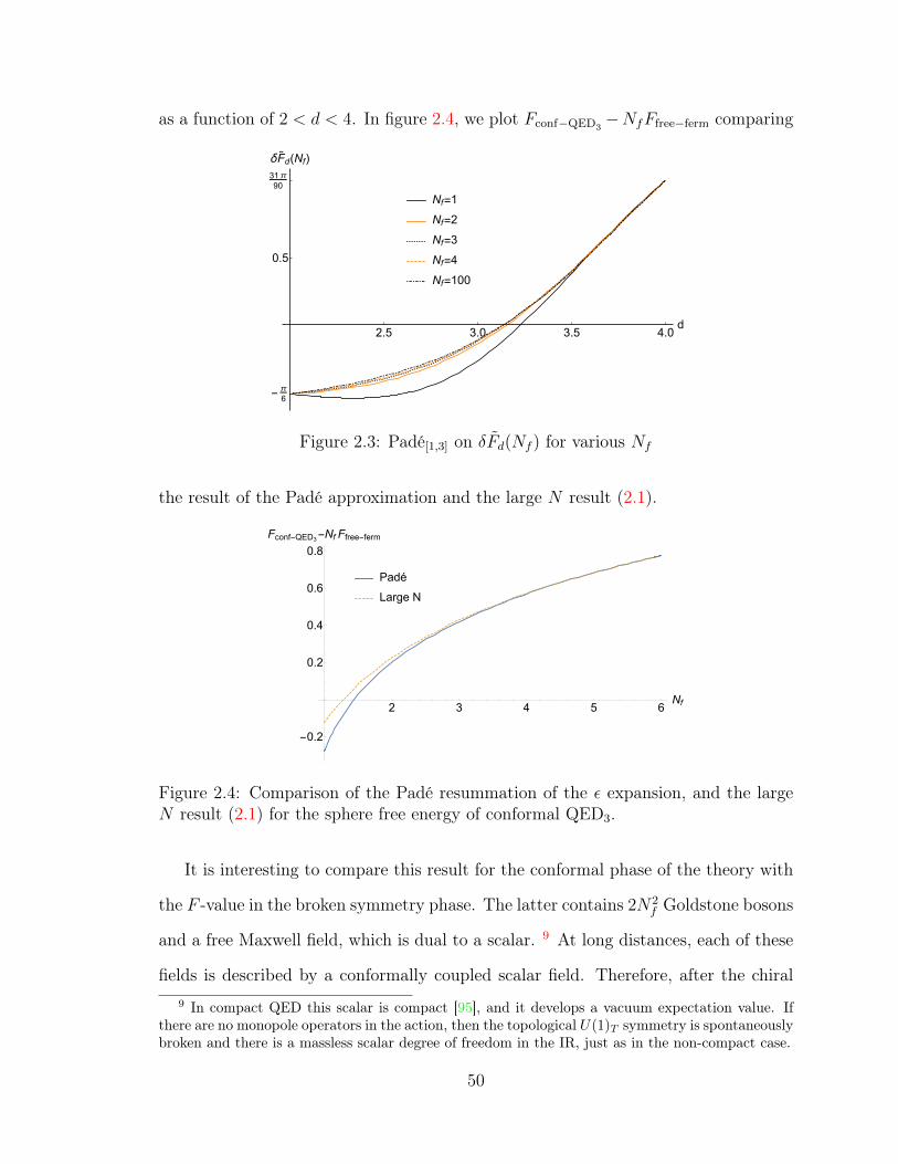
as a function of 2 < d < 4. In figure 2.4, we plot Fconf−QED3−NfFfree−ferm comparing

Nf=1

Nf=2

Nf=3

Nf=4

Nf=100

2.5 3.0 3.5 4.0d

- π6

0.5

31π90

δF˜d(Nf)

Figure 2.3: Padé[1,3] on δFd(Nf ) for various Nf

the result of the Padé approximation and the large N result (2.1).

Padé

Large N

2 3 4 5 6Nf

-0.2

0.2

0.4

0.6

0.8

Fconf-QED3-Nf Ffree-ferm

Figure 2.4: Comparison of the Padé resummation of the ε expansion, and the largeN result (2.1) for the sphere free energy of conformal QED3.

It is interesting to compare this result for the conformal phase of the theory with

the F -value in the broken symmetry phase. The latter contains 2N2f Goldstone bosons

and a free Maxwell field, which is dual to a scalar. 9 At long distances, each of these

fields is described by a conformally coupled scalar field. Therefore, after the chiral9 In compact QED this scalar is compact [95], and it develops a vacuum expectation value. If

there are no monopole operators in the action, then the topological U(1)T symmetry is spontaneouslybroken and there is a massless scalar degree of freedom in the IR, just as in the non-compact case.

50

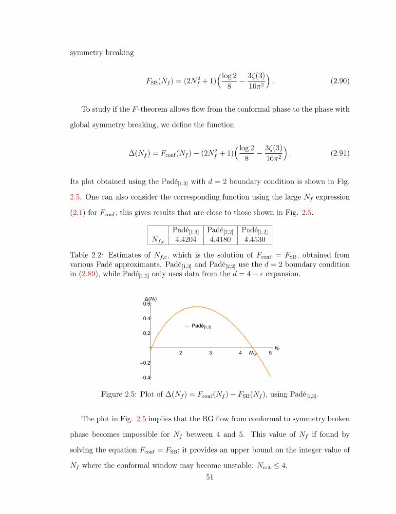
symmetry breaking

FSB(Nf ) = (2N2f + 1)

( log 2

8− 3ζ(3)

16π2

). (2.90)

To study if the F -theorem allows flow from the conformal phase to the phase with

global symmetry breaking, we define the function

∆(Nf ) = Fconf(Nf )− (2N2f + 1)

( log 2

8− 3ζ(3)

16π2

). (2.91)

Its plot obtained using the Padé[1,3] with d = 2 boundary condition is shown in Fig.

2.5. One can also consider the corresponding function using the large Nf expression

(2.1) for Fconf ; this gives results that are close to those shown in Fig. 2.5.

Padé[1,3] Padé[2,2] Padé[1,2]

Nf,c 4.4204 4.4180 4.4530

Table 2.2: Estimates of Nf,c, which is the solution of Fconf = FSB, obtained fromvarious Padé approximants. Padé[1,3] and Padé[2,2] use the d = 2 boundary conditionin (2.89), while Padé[1,2] only uses data from the d = 4− ε expansion.

Padé[1,3]

2 3 4 5Nf,cNf

-0.4

-0.2

0.2

0.4

0.6Δ(Nf)

Figure 2.5: Plot of ∆(Nf ) = Fconf(Nf )− FSB(Nf ), using Padé[1,3].

The plot in Fig. 2.5 implies that the RG flow from conformal to symmetry broken

phase becomes impossible for Nf between 4 and 5. This value of Nf if found by

solving the equation Fconf = FSB; it provides an upper bound on the integer value of

Nf where the conformal window may become unstable: Ncrit ≤ 4.51

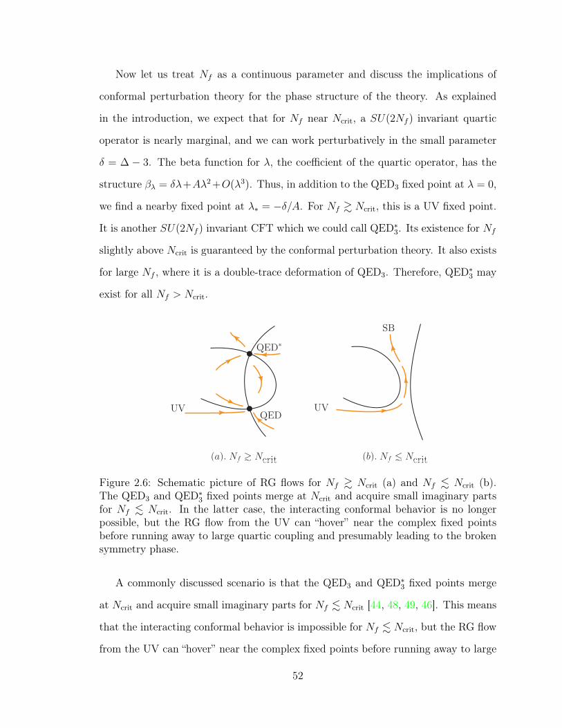
Now let us treat Nf as a continuous parameter and discuss the implications of

conformal perturbation theory for the phase structure of the theory. As explained

in the introduction, we expect that for Nf near Ncrit, a SU(2Nf ) invariant quartic

operator is nearly marginal, and we can work perturbatively in the small parameter

δ = ∆ − 3. The beta function for λ, the coefficient of the quartic operator, has the

structure βλ = δλ+Aλ2 +O(λ3). Thus, in addition to the QED3 fixed point at λ = 0,

we find a nearby fixed point at λ∗ = −δ/A. For Nf & Ncrit, this is a UV fixed point.

It is another SU(2Nf ) invariant CFT which we could call QED∗3. Its existence for Nf

slightly above Ncrit is guaranteed by the conformal perturbation theory. It also exists

for large Nf , where it is a double-trace deformation of QED3. Therefore, QED∗3 may

exist for all Nf > Ncrit.

UV

QED∗

QED

(a). Nf ! Ncrit

SB

UV

(b). Nf " Ncrit

Figure 2.6: Schematic picture of RG flows for Nf & Ncrit (a) and Nf . Ncrit (b).The QED3 and QED∗3 fixed points merge at Ncrit and acquire small imaginary partsfor Nf . Ncrit. In the latter case, the interacting conformal behavior is no longerpossible, but the RG flow from the UV can “hover” near the complex fixed pointsbefore running away to large quartic coupling and presumably leading to the brokensymmetry phase.

A commonly discussed scenario is that the QED3 and QED∗3 fixed points merge

at Ncrit and acquire small imaginary parts for Nf . Ncrit [44, 48, 49, 46]. This means

that the interacting conformal behavior is impossible for Nf . Ncrit, but the RG flow

from the UV can “hover” near the complex fixed points before running away to large

52

quartic coupling and presumably leading to the broken symmetry phase (see figure

2.6). During the hovering F can be made parametrically close to Fconf(Ncrit). This

is why the F -theorem requires Fconf(Ncrit) > FSB (a similar argument involving the

continuity of F was given in [38]). As we have seen, this gives a rather stringent

bound Ncrit . 4.4.

An alternate possibility is that both fixed points stay real and go through each

other. Then the QED3 fixed point continues to exist even after the appearance of a

relevant operator; this relevant operator may create flow from QED3 to the broken

symmetry phase. Therefore, the F -theorem bound on Ncrit is the same as with the

“merger and annihilation” scenario.

2.7 Calculation of CJ1 and CT1

In what follows we calculate the two-point function of the SU(Nf ) current and stress-

energy tensor, which are given by10

Jaν = −ψi(ta)ijγνψj ,

Tµν = −1

4

(ψiγ(µDν)ψ

i −D∗(µψiγν)ψi), (2.92)

where γ(µDν) ≡ γµDν + γνDµ and Dµ = ∂µ + iAµ. Note that there is no Maxwell

term contribution in Tµν , as this term was dropped in (2.47) in the critical limit.

We will work in flat Euclidean d-dimensional metric and introduce a null vector

zµ, which satisfies

z2 = zµzνδµν = 0 . (2.93)

10As it was pointed out in [96], for correlation functions with only gauge invariant operators wecan omit the gauge fixing part and ghost part of the stress-energy tensor. This was explicitly checkedin QCD in d = 4 up to three-loops in [97].

53

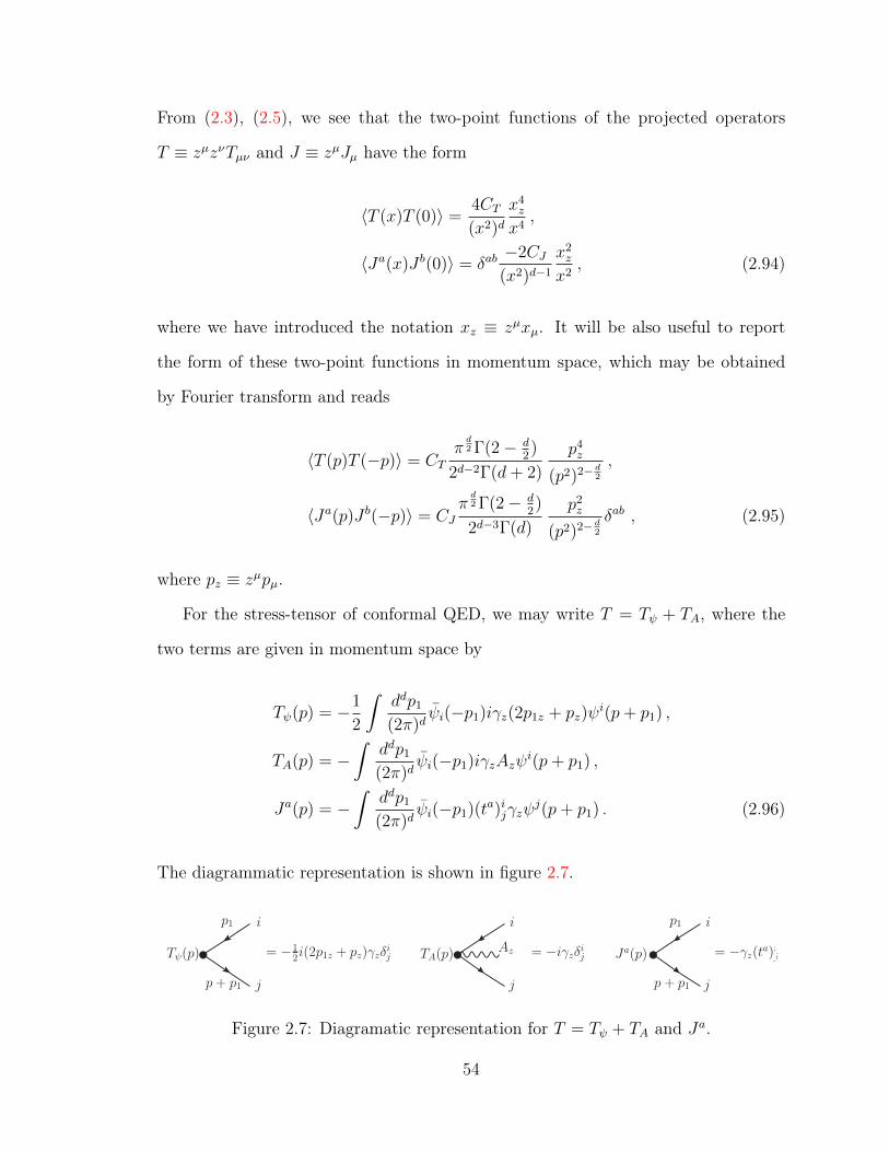
From (2.3), (2.5), we see that the two-point functions of the projected operators

T ≡ zµzνTµν and J ≡ zµJµ have the form

〈T (x)T (0)〉 =4CT(x2)d

x4z

x4,

〈Ja(x)J b(0)〉 = δab−2CJ

(x2)d−1

x2z

x2, (2.94)

where we have introduced the notation xz ≡ zµxµ. It will be also useful to report

the form of these two-point functions in momentum space, which may be obtained

by Fourier transform and reads

〈T (p)T (−p)〉 = CTπd2 Γ(2− d

2)

2d−2Γ(d+ 2)

p4z

(p2)2− d2

,

〈Ja(p)J b(−p)〉 = CJπd2 Γ(2− d

2)

2d−3Γ(d)

p2z

(p2)2− d2

δab , (2.95)

where pz ≡ zµpµ.

For the stress-tensor of conformal QED, we may write T = Tψ + TA, where the

two terms are given in momentum space by

Tψ(p) = −1

2

∫ddp1

(2π)dψi(−p1)iγz(2p1z + pz)ψ

i(p+ p1) ,

TA(p) = −∫

ddp1

(2π)dψi(−p1)iγzAzψ

i(p+ p1) ,

Ja(p) = −∫

ddp1

(2π)dψi(−p1)(ta)ijγzψ

j(p+ p1) . (2.96)

The diagrammatic representation is shown in figure 2.7.

Ja(p)

p1

p + p1

= −γz(ta)i

j

i

j

Tψ(p)

p1

p + p1

= −12i(2p1z + pz)γzδ

ij

i

j

TA(p) = −iγzδij

i

j

Az

Figure 2.7: Diagramatic representation for T = Tψ + TA and Ja.

54

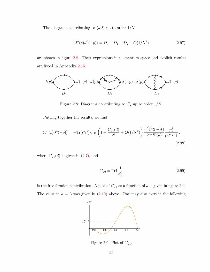
The diagrams contributing to 〈JJ〉 up to order 1/N

〈Ja(p)J b(−p)〉 = D0 +D1 +D2 +O(1/N2) (2.97)

are shown in figure 2.8. Their expressions in momentum space and explicit results

are listed in Appendix 2.16.

J(p) J(−p)

D0 D1 D2

J(p) J(−p)J(p) J(−p)

Figure 2.8: Diagrams contributing to CJ up to order 1/N .

Putting together the results, we find

〈Ja(p)J b(−p)〉 = −Tr(tatb)CJ0

(1 +

CJ1(d)

N+O(1/N2)

)πd2 Γ(2− d

2)

2d−3Γ(d)

p2z

(p2)2− d2

,

(2.98)

where CJ1(d) is given in (2.7), and

CJ0 = Tr11

S2d

(2.99)

is the free fermion contribution. A plot of CJ1 as a function of d is given in figure 2.9.

The value in d = 3 was given in (2.10) above. One may also extract the following

2.0 2.5 3.0 3.5 4.0

7369π2

-8

Figure 2.9: Plot of CJ1.

55

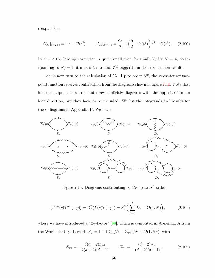
ε-expansions

CJ1|d=2+ε = −ε+O(ε2), CJ1|d=4−ε =9ε

2+

(9

2− 9ζ(3)

)ε2 +O(ε3) . (2.100)

In d = 3 the leading correction is quite small even for small N ; for N = 4, corre-

sponding to Nf = 1, it makes CJ around 7% bigger than the free fermion result.

Let us now turn to the calculation of CT . Up to order N0, the stress-tensor two-

point function receives contribution from the diagrams shown in figure 2.10. Note that

for some topologies we did not draw explicitly diagrams with the opposite fermion

loop direction, but they have to be included. We list the integrands and results for

these diagrams in Appendix B. We have

Tψ(−p)Tψ(p)

D4

Tψ(−p)TA(p)

D3

D0

Tψ(−p)Tψ(p) Tψ(−p)Tψ(p)

D1

D6

TA(−p)TA(p)

D7

TA(p) TA(p)

Tψ(−p)TA(p)

D5

Tψ(−p)Tψ(p)

D2

D8

TA(p) TA(p)

Figure 2.10: Diagrams contributing to CT up to N0 order.

〈T ren(p)T ren(−p)〉 = Z2T 〈T (p)T (−p)〉 = Z2

T

( 8∑n=0

Dn +O(1/N)), (2.101)

where we have introduced a “ZT -factor" [68], which is computed in Appendix A from

the Ward identity. It reads ZT = 1 + (ZT1/∆ + Z ′T1)/N +O(1/N2), with

ZT1 = − d(d− 2)ηm1

2(d+ 2)(d− 1), Z ′T1 = − (d− 2)ηm1

(d+ 2)(d− 1), (2.102)

56

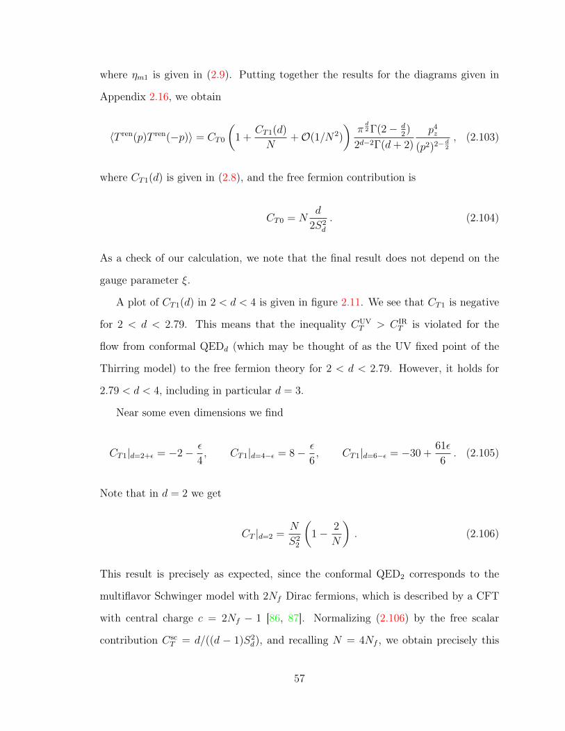
where ηm1 is given in (2.9). Putting together the results for the diagrams given in

Appendix 2.16, we obtain

〈T ren(p)T ren(−p)〉 = CT0

(1 +

CT1(d)

N+O(1/N2)

)πd2 Γ(2− d

2)

2d−2Γ(d+ 2)

p4z

(p2)2− d2

, (2.103)

where CT1(d) is given in (2.8), and the free fermion contribution is

CT0 = Nd

2S2d

. (2.104)

As a check of our calculation, we note that the final result does not depend on the

gauge parameter ξ.

A plot of CT1(d) in 2 < d < 4 is given in figure 2.11. We see that CT1 is negative

for 2 < d < 2.79. This means that the inequality CUVT > CIR

T is violated for the

flow from conformal QEDd (which may be thought of as the UV fixed point of the

Thirring model) to the free fermion theory for 2 < d < 2.79. However, it holds for

2.79 < d < 4, including in particular d = 3.

Near some even dimensions we find

CT1|d=2+ε = −2− ε

4, CT1|d=4−ε = 8− ε

6, CT1|d=6−ε = −30 +

61ε

6. (2.105)

Note that in d = 2 we get

CT |d=2 =N

S22

(1− 2

N

). (2.106)

This result is precisely as expected, since the conformal QED2 corresponds to the

multiflavor Schwinger model with 2Nf Dirac fermions, which is described by a CFT

with central charge c = 2Nf − 1 [86, 87]. Normalizing (2.106) by the free scalar

contribution CscT = d/((d − 1)S2

d), and recalling N = 4Nf , we obtain precisely this

57

central charge. In section 2.9 we will see that CT1|d=4−ε also agrees with the 4 − ε

expansion.

2.0 2.5 3.0 3.5 4.0

-2

-8+ 419245π2

8

Figure 2.11: Plot of CT1.

Near even dimensions the QEDd theory is expected to be described by the free

fermions weakly coupled to a U(1) gauge theory with the local kinetic term (2.11).

For example, in d = 6 this higher-derivative theory was explored in [98, 99, 100, 101,

80, 33, 102]. We may use (2.8) to extract the CT coefficient for the conformal Maxwell

theory (2.11). From (2.8) it follows that

CQEDT1 |even d =

2(−1)d2d!

(d2− 1)!(d

2+ 1)!

= 2(−1)d2

(d

d2− 1

). (2.107)

Recalling that the contribution of the free massless fermions is given by (2.104), we

find that the CT of the conformal Maxwell theory is

Cconf. MaxwellT |even d =

d

2S2d

CQEDT1 |even d = (−1)

d2d

S2d

(d

d2− 1

). (2.108)

In d = 4, 6, 8, 10, . . . this formula gives 16,−90, 448,−2100, . . . times 1/S2d . In d =

4 this agrees with the standard answer for the Maxwell theory. In d = 6, 8, . . .,

eq. (2.108) gives new results for the values of CT in the free conformal theory with

the higher-derivative action (2.11).

58

2.8 CtopJ for the Topological Current in d = 3

In d = 3, it is interesting to compute CtopJ for the “topological" U(1) current

jµtop =i

4πεµνλFνλ , (2.109)

where the factor of i arises because we are working in Euclidean signature, and the

normalization is such that the associated charges are integers. The diagrams con-

tributing to the current two-point function up to order 1/N2 are shown in figure 2.12.

The diagrams D1 and D2 have the same structure as the corresponding ones in fig.

D1 D2

jµtop(p) jν

top(−p)jνtop(−p)jµ

top(p)jµtop(p)

D0

jνtop(−p)

Figure 2.12: Diagrams contributing to CtopJ up to 1/N2 order.

2.9 for the SU(Nf ) current,11 with the difference that at the external points we now

have the gauge U(1) current, to which we attach the two induced photon propagators.

Thus, using the results from Appendix 2.16, we find

〈jµtop(p)jνtop(−p)〉 = − 1

(4π)2εµρσeντλ〈(pρAσ(p)− pσAρ(p))(pτAλ(−p)− pλAτ (−p))〉

= − |p|4π2

CAN

(1− CJ1(3)

N+O(1/N2)

)(δµν −

pµpνp2

), (2.110)

where CA and CJ1(d) are given in (2.49) and (2.7), which yield CA|d=3 = 32 and the

value of CJ1(3) given in (2.100). Therefore, we finally get

〈jµtop(p)jνtop(−p)〉 = − 8|p|π2N

(1 +

1

N

(8− 736

9π2

)+O(1/N2)

)(δµν −

pµpνp2

). (2.111)

11In fact these diagrams can be extracted from the evaluation of the polarization operator, whichwas computed in case of QCD in [103].

59

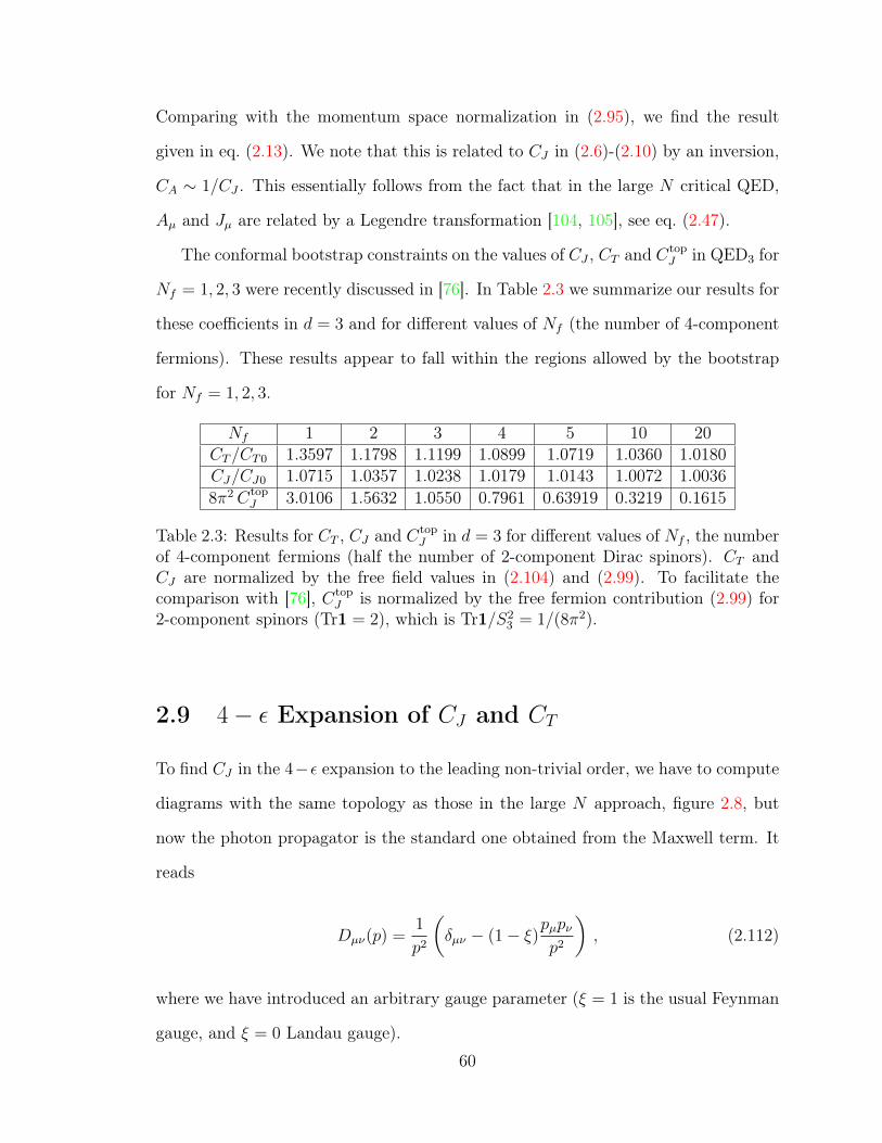
Comparing with the momentum space normalization in (2.95), we find the result

given in eq. (2.13). We note that this is related to CJ in (2.6)-(2.10) by an inversion,

CA ∼ 1/CJ . This essentially follows from the fact that in the large N critical QED,

Aµ and Jµ are related by a Legendre transformation [104, 105], see eq. (2.47).

The conformal bootstrap constraints on the values of CJ , CT and CtopJ in QED3 for

Nf = 1, 2, 3 were recently discussed in [76]. In Table 2.3 we summarize our results for

these coefficients in d = 3 and for different values of Nf (the number of 4-component

fermions). These results appear to fall within the regions allowed by the bootstrap

for Nf = 1, 2, 3.

Nf 1 2 3 4 5 10 20CT/CT0 1.3597 1.1798 1.1199 1.0899 1.0719 1.0360 1.0180CJ/CJ0 1.0715 1.0357 1.0238 1.0179 1.0143 1.0072 1.00368π2Ctop

J 3.0106 1.5632 1.0550 0.7961 0.63919 0.3219 0.1615

Table 2.3: Results for CT , CJ and CtopJ in d = 3 for different values of Nf , the number

of 4-component fermions (half the number of 2-component Dirac spinors). CT andCJ are normalized by the free field values in (2.104) and (2.99). To facilitate thecomparison with [76], Ctop

J is normalized by the free fermion contribution (2.99) for2-component spinors (Tr1 = 2), which is Tr1/S2

3 = 1/(8π2).

2.9 4− ε Expansion of CJ and CT

To find CJ in the 4−ε expansion to the leading non-trivial order, we have to compute

diagrams with the same topology as those in the large N approach, figure 2.8, but

now the photon propagator is the standard one obtained from the Maxwell term. It

reads

Dµν(p) =1

p2

(δµν − (1− ξ)pµpν

p2

), (2.112)

where we have introduced an arbitrary gauge parameter (ξ = 1 is the usual Feynman

gauge, and ξ = 0 Landau gauge).

60

The renormalization of the electric charge is well-known, and in minimal subtrac-

tion scheme it reads [15]:

e0 = µε2

(e+

4Nf

3ε

e3

(4π)2+(8N2

f

3ε2+

2Nf

ε

) e5

(4π)4+ . . .

), (2.113)

where e is the renormalized coupling, and the corresponding beta function is

β = − ε2e+

4Nf

3

e3

(4π)2+

4Nfe5

(4π)4− 2Nf (22Nf + 9)

9

e7

(4π)6+ . . . . (2.114)

Then, one finds an IR stable perturbative fixed point at

e∗ = π

√6ε

Nf

(1− 9

16Nf

ε+3(44Nf + 207)

512N2f

ε2 +O(ε3)

). (2.115)

Computing the diagrams in figure 2.8 with the photon propagator (2.112), taking a

Fourier transform to coordinate space, and setting e = e∗ at the end, we obtain in

d = 4− ε

CJ/CfreeJ = 1 +

9ε

8Nf

+O(1/N2f ) . (2.116)

which precisely agrees with (2.100) (recall that in this case we have N = NfTr1 =

4Nf ).

To calculate the 4 − ε expansion of CT to order ε, we will use as a shortcut the

fact that in d = 4 the CT coefficient may be obtained as (see e.g. [106, 107])

CT =640

π2βa , (2.117)

where βa is the beta function for the Weyl-squared term, which is known to be [61, 59]

βa =Nf + 2

20(4π)2+

7Nf

36

e2

(4π)4+ . . . . (2.118)

61

The first term corresponds to the contributions of the free fermions and of the Maxwell

field, while the second one encodes the leading interaction corrections. The second

term, when evaluated at the IR fixed point (2.115) in d = 4−ε, gives 7ε6(16π)2 . However,

this is not the only contribution of order ε because the free field contributions need to

be evaluated in 4− ε dimensions. The contribution of free massless fermions is given

in (2.104). The contribution of the Maxwell field is more subtle, since this theory is

scale invariant but not conformal away from four dimensions [11]. However, defining

the projected stress-tensor TMaxwell = zµzνFµαFαν (this selects the traceless part of

Tµν), and using the field strength two-point function [11]

〈Fµν(x)Fρσ(0)〉 =(2d− 4)Γ

(d2− 1)

4πd2 (x2)d/2

[(δµρ −

d

2

xµxρx2

)(δνσ −

d

2

xνxσx2

)− µ↔ ν

](2.119)

we find that 〈TMaxwell(x)TMaxwell(0)〉 takes the form (2.94), just as in a conformal field

theory, with the normalization given by

CMaxwellT =

d2(d− 2)

2S2d

. (2.120)

This serves as the natural definition of CT for the Maxwell theory (in d = 4, it agrees

with the well-known result [66]). Putting these results together we find

CQEDT = C free ferm

T

(1 +

d(d− 2) + 35ε/6

N+ . . .

)= C free ferm

T

(1 +

8− ε/6N

+ . . .

),

(2.121)

which exactly agrees with (2.105). This gives a highly non-trivial test of the dimension

dependence of CT1.

62

2.10 Another Estimate for Symmetry Breaking in

QED3

In d = 3, the QED Lagrangian has SU(2Nf ) global symmetry. For Nf < Nf,crit it may

be broken via the generation of vacuum expectation value of the operator∑Nf

j=1 ψjψj

(this is written using the 4-component spinors ψi and gamma-matrices) [21, 14]. This

operator preserves the 3-d time reversal symmetry, but it breaks the global symmetry

to SU(Nf )× SU(Nf )× U(1).

In an earlier paper [33], using the F -theorem inequality FUV > F IR [34, 36, 37,

35, 51] we showed that theories with Nf = 5 and higher must be in the conformal

phase. The F -theorem method is inconclusive, however, for theories with Nf ≤ 4.

There is lattice evidence that theories with Nf = 1, 2 are not conformal [64, 65],12

but little is known about theories with Nf = 3, 4.

Let us now consider a different RG inequality:

CUVT > CIR

T , (2.122)

which is sometimes called “the CT theorem". While there is a known d = 3 counter-

example to this inequality [77], which involves theories with N = 2 supersymmetry,

many known RG flows appear to obey (2.122). For example, it is obeyed for flows

involving the scalar O(N) [67, 68] and the Gross-Neveu model [68]. If we think of

the conformal QED3 theory as the UV fixed point of the Thirring model, then the

inequality (2.122) is obeyed by the flow to the free fermion theory because CT1(3) > 0.

We may also test this inequality for the flow from the QED theory in the extreme

UV, which consists of the free decoupled Maxwell field and Nf 4-component fermions,12See, however, the recent lattice work [108] suggesting that they are conformal.

63

to the conformal QED3. For the former we find using (2.120) and (2.104)

CUVT =

12Nf + 9

32π2. (2.123)

For the interacting conformal phase, using our result (2.10), we have

CIRT =

6Nf

16π2

(1 +

419245π2 − 8

4Nf

+O(1/N2f )

). (2.124)

We see that at large Nf (2.122) is obeyed to order N0f because 9 > 3

(419245π2 − 8

)≈ 4.32.

Let us now try applying (2.122) to the d = 3 flow from QED in the extreme UV

to the broken symmetry phase. For the former we have (2.123). The latter is a free

conformal field theory of 2N2f + 1 scalar fields; therefore, it has

CIRT =

3(2N2f + 1)

32π2. (2.125)

We find that the two expressions are equal for Nf = Nf,crit = 1 +√

2 ≈ 2.414. This

suggests that theories with Nf = 3 and higher are in the conformal phase. The

inequality (2.122), however, does not require the Nf = 1, 2 theories to be conformal,

and indeed there is lattice evidence that they are not [64, 65].13

2.11 CT for Large Nf QCDd

To the leading nontrivial order, the large Nf computations for QCD look similar to

those in the QED case. The results for large Nf QCD at the critical point can be13 A more stringent value Nf,crit = 3/2 follows from the RG inequality based on the coefficient

of the thermal free energy [109]. This appears to be in contradiction with the lattice gauge theorywork [65] claiming that the Nf = 2 theory is not conformal. However, both Nf,crit = 3/2 andNf,crit = 1 +

√2 ≈ 2.414 are consistent with the recent paper [108] claiming that the symmetry

breaking does not take place even for Nf = 1.

64

deduced from the lagrangian [110, 111, 102, 112, 113, 114, 103, 73, 115]

Lcrit QCD = −ψiγµ(∂µ + iAaµta)ψi +

Nf

2ξ((d−4)/2∂A)2 + ∂µc

a∂µca + fabc∂µcaAbµcc ,

(2.126)

where ψi with i = 1, .., Nf are the quark fields belonging to the fundamental represen-

tation of the colour group G, Aaµ is the gluon field and ca and ca are the ghost fields

in the adjoint representation of the colour group. We will use the following notation

for the Casimirs of the Lie group generators ta ([ta, tb] = ifabctc):

Tr(tatb) = C(r)δab, tata = C2(r) · I, facdf bcd = C2(G) · I (2.127)

and also tr(I) = d(r) and δabδab = d(G). The stress-energy tensor is (2.92) with

Dµ = ∂µ + iAaµta, and as we mentioned above we can omit the gauge fixing and ghost

parts of Tµν when computing correlation functions of gauge invariant operators. The

diagrams contributing to CT to order 1/Nf are the same as in the QED case (see figure

2.10). It is not hard to show that the relations between QED and QCD diagrams are

DQCD0 = d(r)DQED

0 , DQCDn = d(G)DQED

n , n = 1, .., 8 , (2.128)

where for some diagrams we used the identity d(r)C2(r) = d(G)C(r). Therefore, we

find

CQCDT = d(r)CT0

(1 +

1

N

d(G)

d(r)CT1 +O(1/N2)

), (2.129)

65

where CT0 and CT1 are the results for QED given in (2.104) and (2.8). For SU(Nc)

gauge group we have d(r) = Nc and d(G) = N2c − 1, thus

CQCDT = NcCT0

(1 +

1

N

N2c − 1

Nc

CT1 +O(1/N2)

). (2.130)

Let us check that this agrees with the known exact result for central charge in

d = 2 gauge theory with massless flavors. The conformal limit of SU(Nc) gauge

theory has central charge [85, 86, 87, 116]

c = cfree −(N2

c − 1)k

k +Nc

. (2.131)

The subtraction of the second term is due to the gauging of the SU(Nc) Kac-Moody

algebra with level k. Since there are 2Nf 2-d Dirac flavors in the fundamental

representation of SU(Nc), we have k = 2Nf . This theory may be described by a

SU(2Nf )Nc × U(1) WZW model [86, 87]. Its central charge is

c = 2Nf2NfNc + 1

2Nf +Nc

= NfNc −2(N2

c − 1)Nf

2Nf +Nc

= 2NfNc

(1− 1

2Nf

N2c − 1

Nc

+ . . .

),

(2.132)

which is in agreement with (2.130) evaluated in d = 2. For a general gauge group G

we have

c = 2Nfd(r)− 2d(G)Nf

2Nf + d(r)= 2Nfd(r)

(1− 1

2Nf

d(G)

d(r)+ . . .

), (2.133)

which agrees with (2.129). Analogously, one can easily see that we have the same

relation between CJ in QCD and QED:

CQCDJ = d(r)CJ0

(1 +

1

N

d(G)

d(r)CJ1 +O(1/N2)

), (2.134)

66

where CJ0 and CJ1 are the results for QED given in (2.99) and (2.7). The value of CT

for the d = 6 conformal Maxwell theory was calculated directly in [117]. The result

is in agreement with our (2.108), providing a check of our methods.

2.12 Appendix A. Eigenvalues of the kernel Kµν

On the Sd in stereographical coordinates the kernel Kµν = −〈JµJν〉 has the form

Kµν(x, y) = −CJ4R2

(1 + x2)(1 + y2)

(δµν − 2 (x−y)µ(x−y)ν

|x−y|2)

s(x, y)2∆. (2.135)

We need to decompose the kernel on a sum of vector spherical harmonics:

Kµν(x, y) =∑`,m

∑s

λ(s)` Y

(s)∗µ,`m(x)Y

(s)ν,`m(y) , (2.136)

where s denotes different types of vector spherical harmonics, ` is the principal angular

quantum number and the range of m for given ` and s is g(s)` (see (2.20)-(2.21)). The

eigenvalue λ(s)` has no m dependence because of rotational invariance. Because of

vector spherical harmonics are orthonormal to each other we have14

λ(s)` =

∫ddxddy

√gx√gyK

µν(x, y)Y(s)µ,`m(x)Y

(s)∗ν,`m(y) . (2.137)

We first consider longitudinal vector harmonics [78]

Y(0)µ,`m(x) =

∇µY`m(x)√`(`+ d− 1)

, (2.138)

14We assume that∫ddx√gxY

(s)∗µ,`m(x)Y

µ(s′)`′m′ (x) = δ``′δmm′δss′ .

67

where Y`m(x) are usual scalar spherical harmonics15. Integrating by parts in (2.137)

we get

λ(0)` =

1

`(`+ d− 1)

∫ddxddy

√gx√gy∇µ∇νK

µν(x, y)1

g(0)`

∑m

Y`m(x)Y ∗`m(y) , (2.139)

where we sum over m and divide by the degeneracy g(0)`

16. We use that 17

1

g(0)`

∑m

Y`m(x)Y ∗`m(y) =1

vol(Sd)C

(d−1)/2` (1− s2(x, y)/2R2)

C(d−1)/2` (1)

, (2.140)

where C(d−1)/2` (x) is the Gegenbauer polynomial. Now due to rotational invariance

we may choose y = 0 and find18

∇µ∇νKµν(x, 0) = − 2CJ

(4R2)∆+1(∆− d+ 1)(2− d+ 2∆ + x2d)

(1 + x2)∆

(x2)∆+1. (2.141)

Therefore we obtain

λ(0)` =− CJ(∆− d+ 1)

2∆R2∆−d`(d+ `− 1)

vol(Sd−1)

C(d−1)/2` (1)

×∫ 1

−1

dz(1 + z)d−2

2 (1− z)d2−∆−2(2 + 2∆− d− (1− z)(1 + ∆− d))C

(d−1)/2` (z) ,

(2.142)

15We assume that ∇2Y`m = −`(`+ d− 1)R−2Y`m and∫ddx√gxY`m(x)Y ∗`′m′(x) = δ``′δmm′ .

16We are allowed to do this sum because on the l.h.s λ(0)` doesn’t depend on m.

17Notice that the Y`m(x) harmonics have a factor of R−d/2, which is consistent with the formula(2.140) because vol(Sd) = 2π

d+12 Rd/Γ(d+1

2 ) and Y (s)µ,`m have a factor of R−d/2+1.

18Notice that we can not just take y = 0 in (2.139) without having the sum over m.

68

where we have changed the variable x2 = (1− z)/(1 + z). Calculating the integral we

get19

λ(0)` = −CJ

2d−2∆πd/2(∆− 1)Γ(d2−∆

)Γ(∆ + 1)

d−∆− 1

∆− 1

Γ(l + ∆)

Γ(d+ l −∆)

1

R2∆−d . (2.143)

The eigenvalues λ(1)` for transverse spherical harmonics can be easily found for

∆ = d− 1, using the embedding formalism. In this case the kernel has the form [60]

Kab(η1, η2) = −CJR−2

(2d− 4)(d− 1)Pac

δcb|η1 − η2|2d−4

, (2.144)

where the operator Pac ≡ 12L2δac +LadLdc− (d− 1)Lac acts on η1, and Lab ≡ ηa

∂∂ηb−

ηb∂∂ηa

and L2 ≡ LabLab . Now using the decomposition [60]

δcb|η1 − η2|2d−4

=∑l,m

∑s

(2R)4−dπd2

Γ(2− d2)Γ(`+ d− 2)

Γ(d− 2)Γ(`+ 2)Y

(s)c,`m(η1)Y

(s)b,`m(η2) (2.145)

and the property of the operator Pab: PabY(s)b,`m = 0 for s 6= 1 and PabY

(1)b,`m = −(` +

1)(`+ d− 2)Y(1)a,`m, we find

Kab(η1, η2) =∑`,m

CJ(2R)4−dπ

d2 (`+ 1)(`+ d− 2)Γ(2− d

2)Γ(`+ d− 2)

R2(2d− 4)(d− 1)Γ(d− 2)Γ(`+ 2)Y

(1)a,`m(η1)Y

(1)b,`m(η2) ,

(2.146)

therefore for λ(1)` we get

λ(1)` = CJ

πd2 Γ(2− d

2

)Γ(`+ d− 1)

2d−3Γ(d)Γ(`+ 1)

1

Rd−2, (2.147)

19Here we used the integral∫ 1

−1dz(1 + z)ν−

12 (1 − z)βCν` (z) =

(−1)`2β+ν+ 1

2 Γ(β+1)Γ(ν+ 12 )Γ(2ν+l)Γ(β−ν+ 3

2 )

`!Γ(2ν)Γ(β−ν−`+ 32 )Γ(β+ν+`+ 3

2 ), which can be found with the help of [118] 7.311.3

and the relation Cν` (z) = (−1)`Cν` (−z). Also we used that Cd−1

2

` (1) = (`+d−2)!`!(d−2)! .

69

which coincides with (2.54) for ∆ = d− 1.

2.13 Appendix B. Zonal spherical harmonics in con-

tinuous dimesion

In this appendix we give more detailed derivation of the formula (2.54). As we already

saw in the case of the conformal QED on the sphere in some physical computations

one encounters a problem of decomposition of some kernel on the sphere Sd into a

sum over tensor spherical harmonics [119, 83, 120]. In general it is quite difficult

task to perform analytically. But in many cases the kernel in question has rotational

invariance, which drastically simplifies the calculations.

We consider a decomposition of some general kernel

Kµ1....µr,ν1....νr(n, n′) =

∑`,m,s

λ(s)` Y

(s)µ1...µr,`m

(n)Y(s)∗ν1,...,νr,`m

(n′) , (2.148)

where n, n′ are vectors on the sphere with unit radius, and Y (s)µ1...µr,`m

are tensor spher-

ical harmonics of type s. The eigenvalues λ(s)` depend only on ` due to rotational

invariance of K 20 and have degeneracy g(s)` .

Since all tensor spherical harmonics orthonormal to each other21

∫ddnY

(s)µ1...µr,`m

(n)Yµ1...µr,(s′)∗`′m′ (n) = δ``′δmm′δss′ (2.149)

we find for the eigenvalues

λ(s)` =

∫ddnddn′Kµ1....µr,ν1....νr(n, n′)Y

(s)µ1...µr,`m

(n)Y(s)∗ν1,...,νr,`m

(n′) . (2.150)

20This means that Kµ1...µr;ν1...νr depends only on z = n · n′ or equivalentlyKµ1...µr;ν1...νr (On,On

′) = Oα1µ1...OαrµrO

β1ν1...OβrνrKα1...αr;β1...βr (n, n

′), where O is orthogonal matrix21Here the summation over indices µ1, ..., µr is assumed. The indices are raised and lowered by

metric tensor gµν on the sphere.

70

We can sum over m in the r.h.s of (2.150) and divide by the degeneracy of m: g(s)` ,

so we get

λ(s)` =

1

g(s)`

∫ddnddn′Kµ1....µr,ν1....νr(n, n′)Z

(s)µ1...µr,ν1...νr,`

(n, n′) , (2.151)

where we have introduced tensor zonal harmonics of spin s:

Z(s)µ1...µr,ν1...νr,`

(n, n′) ≡∑m

Y(s)µ1...µr,`m

(n)Y(s)∗ν1,...,νr,`m

(n′) . (2.152)

The important property of Z(n, n′) is that it is rotational invariant and thus depends

only on z = n · n′. Therefore in the integral (2.151) we may put n′ to the north pole

and integrate only over the angle between n and n′[83]:

λ(s)` =

vol(Sd)vol(Sd−1)

g(s)`

∫ 1

−1

dz(1− z2)d2−1Kµ1....µr,ν1....νr(z)Z

(s)µ1...µr,ν1...νr,`

(z) . (2.153)

Also we notice that zonal harmonics obey completeness condition

∑s

∑`

Z(s)µ1...µr,ν1...νr,`

(n, n′) = gµ1ν1 ...gµrνrδ(n− n′) . (2.154)

In the next subsections we find the explicit expressions for the tensor zonal spherical

harmonics of rank zero and one.

2.13.1 Rank 0 zonal harmonics

In scalar case the zonal harmonics are known

Z`(n, n′) =

∑m

Y`m(n)Y ∗`m(n′) ≡ g`vol(Sd)

C(d−1)/2` (n · n′)C

(d−1)/2` (1)

, (2.155)

71

where C(d−1)/2` (z) is the Gegenbauer polynomial and g` is degeneracy of m in scalar

case.

2.13.2 Rank 1 zonal harmonics

In vector case we have two types of the vector spherical harmonics. One type is

longitudinal harmonics, for which we know the explicit form in terms of the scalar

harmonics [121]

Y(0)µ,`m =

∇µY`m√`(`+ d− 1)

. (2.156)

The other type is the transverse vector harmonics Y (1)µ,`m, ∇µY

(1)µ,`m = 0. The explicit

form for the transverse vector harmonics is not known. Using that −∇2Y`m = `(` +

d− 1)Y`m we can find

Z(0)µ,ν′,`(n, n

′) =1

`(`+ d− 1)

∑m

∇µY`m(n)∇ν′Y∗`m(n′) = −∇µ∇ν′

1

∇2Z`(n, n

′) .

(2.157)

Let us now try to find Z(1)µ,ν,`(n, n

′). We know that it depends only on z = n · n′,

and it must obey the equation

−∇2Z(1)µ,ν′,`(n, n

′) = (`(`+ d− 1)− 1)Z(1)µ,ν′,`(n, n

′) . (2.158)

and the same for −∇′2 (but it is automaticaly fulfilled, because everything depends

only on the relative angle between n and n′). Also we must have ∇µZ(1)µ,ν′,`(n, n

′) =

∇ν′Z(1)µ,ν′,`(n, n

′) = 0.

72

2.13.3 Computations in stereographical coordinates

We consider the sphere of unit radius. In the stereographical coordinates the metric

on the sphere is

gµν =4δµν

(1 + x2)2, gµν =

(1 + x2)2

4δµν . (2.159)

One can find the Cristoffel symbols

Γλµν = − 2

(1 + x2)(xµδλν + xνδλµ − xλδµν) , (2.160)

therefore

Γνµν = − 2d xµ(1 + x2)

, Γλµµ =2(d− 2)

1 + x2xλ . (2.161)

The Riemann and Ricci tensors are given by the expressions

Rµνλρ = gµλgνρ − gνλgµρ, Rµν = (d− 1)gµν (2.162)

and one can find for the Laplacian of the scalar

∇2φ =(1 + x2)2

4

(∂2µ −

2(d− 2)

1 + x2xµ∂µ

)φ . (2.163)

We denote the chordal distance by s(x, y):

u = s(x, y)2 =4(x− y)2

(1 + x2)(1 + y)2, (2.164)

where (x− y)2 = δµν(x− y)µ(x− y)ν . Then we have for z = n · n′:

z = 1− 1

2s(x, y)2 . (2.165)

73

We will use the following formulas22

∇2z = −dz ,

(∂µz)(∂µz) = 1− z2 ,

∇µ∂νz = −gµνz ,

(∂µz)(∇µ∂ν∂ν′z) = −(∂νz)(∂ν′z) ,

(∂µz)(∂µ∂ν′z) = −z∂ν′z ,

(∂µ∂µ′z)(∂µ∂ν′z) = gµ′ν′ − (∂µ′z)(∂ν′z) ,

∇µ∂ν∂ν′z = −gµν∂ν′z . (2.166)

And the additional identity

zµµ′zµνν′ = −zνµ′zν′ , (2.167)

where zµ1...µnν′1...ν′n≡ ∇µ1 ...∇µn∇ν′1

...∇ν′nz.

For the longitudinal zonal harmonics we find

Z(0)µν′,`(u) = − 1

`(`+ d− 1)

(∂µz∂ν′zZ

′′` (z) + ∂µ∂ν′zZ

′`(z)

). (2.168)

Using that

Z`(u) =g

(0)`

vol(Sd)C

(d−1)/2` (z)

C(d−1)/2` (1)

, (2.169)

22One has ∂µu = 2u(

(x−y)µ(x−y)2 − xµ

1+x2

), ∂ν′u = 2u

((y−x)ν′(x−y)2 − yν′

1+y2

)

74

and also that ∂zCα` (z) = 2αCα+1

`−1 (z) we may write23

Z(0)µν′,`(z) =

g(0)`

dC(d+1)/2`−1 (1)vol(Sd)

(∂µz∂ν′z(d+ 1)C

(d+3)/2`−2 (z) + ∂µ∂ν′zC

(d+1)/2`−1 (z)

).

(2.170)

Now to find Z(1)µν′,`(z) we adopt the following ansatz

Z(1)µν′,`(z) = ∂µz∂ν′zA`(z) + ∂µ∂ν′zB`(z) . (2.171)

We can find functions A and B by solving the eqauations for Z(1)µν′,`(u):

∇2Z(1)µν′,`(z) = −(`(`+ d− 1)− 1)Z

(1)µν′,`(z) ,

∇µZ(1)µν′,`(z) = 0 . (2.172)

We find

∇2(∂µ∂ν′zB`) =((1− z2)B′′` − dzB′` −B`

)∂µ∂ν′z − 2∂µz∂ν′zB

′` ,

∇µ(∂µ∂ν′zB`) = −∂ν′z(zB′` + dB`) (2.173)

and also

∇2(∂µz∂ν′zA`) =((1− z2)A′′` − (d+ 4)zA′` − (d+ 1)A`

)∂µz∂ν′z − 2z∂µ∂ν′zA` ,

∇µ(∂µz∂ν′zA`) = ∂ν′z((1− z2)A′` − (d+ 1)zA`

). (2.174)

23We use that C(d−1)/2` (1) = (`+d−2)!

`!(d−2)!

75

So we obtain

(1− z2)A′` − (d+ 1)zA` − zB′` − dB` = 0 ,

(1− z2)A′′` − (d+ 4)zA′` − (d+ 1)A` − 2B′` = −(`(`+ d− 1)− 1)A` ,

(1− z2)B′′` − dzB′` −B` − 2zA` = −(`(`+ d− 1)− 1)B` . (2.175)

The explicit result in d = 3 helps to find the exact solution of these equations

A` = c((d+ 1)zC

(d+3)/2`−2 (z) + (d− 1)C

(d+1)/2`−1 (z)

),

B` = c((d+ 1)(1− z2)C

(d+3)/2`−2 (z)− (d− 1)zC

(d+1)/2`−1 (z)

)(2.176)

and Z(1)µν′,`(z) = ∂µz∂ν′zA`(z) + ∂µ∂ν′zB`(z). We can find normalization constant c by

considering zonal harmonics for n = n′, so in general we have

∫ddnZ

(s),µ1...µrµ1...µr,`

(1) =∑m

∫ddnY

(s)µ1...µr,`m

(n)Yµ1...µr,(s)∗`m (n) = g

(s)` , (2.177)

therefore

Z(s),µ1...µrµ1...µr,`

(1) =g

(s)`

vol(Sd). (2.178)

In case of rank 1 we have

Z(1),µµ,` (1) = dB`(1) =

g(1)`

vol(Sd)(2.179)

where we used that gµν′∂µz∂ν′z|z=1 = 0 and gµν′∂µ∂ν′z|z=1 = d. Thus we find

c = − g(1)`

d(d− 1)C(d+1)/2`−1 (1)vol(Sd)

. (2.180)

76

Therefore finally we have

Z(1)µν′,`(z) =− g

(1)`

d(d− 1)C(d+1)/2`−1 (1)vol(Sd)

(∂µz∂ν′z

((d+ 1)zC

(d+3)/2`−2 (z) + (d− 1)C

(d+1)/2`−1 (z)

)+ ∂µ∂ν′z

((d+ 1)(1− z2)C

(d+3)/2`−2 (z)− (d− 1)zC

(d+1)/2`−1 (z)

)). (2.181)

2.13.4 Rank 1 kernel decomposition

We have the following kernel in stereographical coordinates

Kµν′(x, y) = −CJ4

(1 + x2)(1 + y2)

(δµν′ − 2

(x−y)µ(x−y)ν′|x−y|2

)s(x, y)2∆

, (2.182)

We put y = 0 and get

Kµν′(x, 0) = −CJ(1 + x2)∆+1

4∆+1(x2)∆

(δµν′ − 2

xµxν′

x2

). (2.183)

Then one can find at y = 0:

∂µz = − 4xµ(1 + x2)2

, ∂ν′z =4xν′

1 + x2,

∂µz∂ν′z = − 42xµxν′

(1 + x2)3, ∂µ∂ν′z =

4

1 + x2

(δµν′ −

2xµxν′

1 + x2

). (2.184)

Therefore we obtain

Kµν′(x, 0)∂µz∂ν′z = −CJ2−∆(1− z)−∆+1(1 + z) ,

Kµν′(x, 0)∂µ∂ν′z = CJ2−∆(1− z)−∆(1 + z − d) , (2.185)

where we used that x2 = (1− z)/(1 + z). Then we have

λ(s)` =

vol(Sd)vol(Sd−1)

g(s)`

∫ 1

−1

dz(1− z2)d2−1Kµ,ν′(z)Z

(s)µ,ν′,`(z) , (2.186)

77

where [122, 78, 123]

g(0)` =

(2`+ d− 1)(`+ d− 2)!

`!(d− 1)!, g

(1)` =

`(`+ d− 1)(2`+ d− 1)(`+ d− 3)!

(d− 2)!(`+ 1)!.

(2.187)

Using expressions (2.170) and (2.181) we find

λ(0)` =

CJ2−∆vol(Sd−1)

dC(d+1)/2`−1 (1)

(1 + ∆− d)

∫ 1

−1

dz(1 + z)d2 (1− z)

d2−∆−1C

(d+1)/2`−1 (z),

λ(1)` = − CJ2−∆vol(Sd−1)

d(d− 1)C(d+1)/2`−1 (1)

(d− 1)(∆− 1)

∫ 1

−1

dz(1 + z)d2 (1− z)

d2−∆−1C

(d+1)/2`−1 (z) .

(2.188)

Calculating the integrals we finally get24

λ(0)` = −CJ

2d−2∆πd/2(∆− 1)Γ(d2−∆

)Γ(∆ + 1)

Γ (`+ ∆)

Γ (`+ d−∆)

d− 1−∆

∆− 1,

λ(1)` = −CJ

2d−2∆πd/2(∆− 1)Γ(d2−∆

)Γ(∆ + 1)

Γ (`+ ∆)

Γ (`+ d−∆). (2.189)

which is in agreement with (2.54).

2.14 Appendix C. Calculation of G2 and G4

Using the propagators and vertex in (2.80),(2.79), (2.78) we find for the two-point

function

G2 = −Nf

∫ddη1d

dη2 Tr(Qab(η1)αbS(η1, η2)Qcd(η2)αdS(η2, η1))Dac(η1, η2) . (2.190)

24Here we used the integral∫ 1

−1dz(1 + z)ν−

12 (1 − z)βCν` (z) =

(−1)`2β+ν+ 1

2 Γ(β+1)Γ(ν+ 12 )Γ(2ν+l)Γ(β−ν+ 3

2 )

`!Γ(2ν)Γ(β−ν−`+ 32 )Γ(β+ν+`+ 3

2 ), which can be found with the help of [118] 7.311.3

and the relation Cν` (z) = (−1)`Cν` (−z).

78

After calculation we obtain

G2 = −(NfTr1)Γ(d2)Γ(d− 2)

2d+2π3d2 Rd−2

∫ddη1d

dη2

(d− 2 + 1

2R2 (η1 − η2)2)

|η1 − η2|2d−2 2F1(1, d− 2,d

2, 1− (η1 − η2)2

4R2) .

(2.191)

Due to rotational invariance we can put η2 to the north pole of the sphere and get in

stereographic coordinates

G2 = −(NfTr1)R4−dΓ(d− 2)

(16π)d−1

2 Γ(d+1

2

) ∫ ∞0

dx

(1 + x2)xd−1

(d− 2

1 + x2

)2F1(1, d− 2,

d

2,

1

(1 + x2)) .

(2.192)

Now introducing the variable z = 1/(1 + x2) we find

G2 = −(NfTr1)R4−dΓ(d− 2)

2(16π)d−1

2 Γ(d+1

2

) ∫ 1

0

dzzd2−1(1− z)−

d2 (d− 2z) 2F1(1, d− 2,

d

2, z) .

(2.193)

The integral can be calculated exactly and we obtain25

G2 = − (NfTr1)R4−dΓ(d− 1)

(d− 3)4d+2

2 (4π)d−3

2 sin(πd2

)Γ(d+1

2

) . (2.194)

25G2 was also computed in [62, 63] by different methods.

79

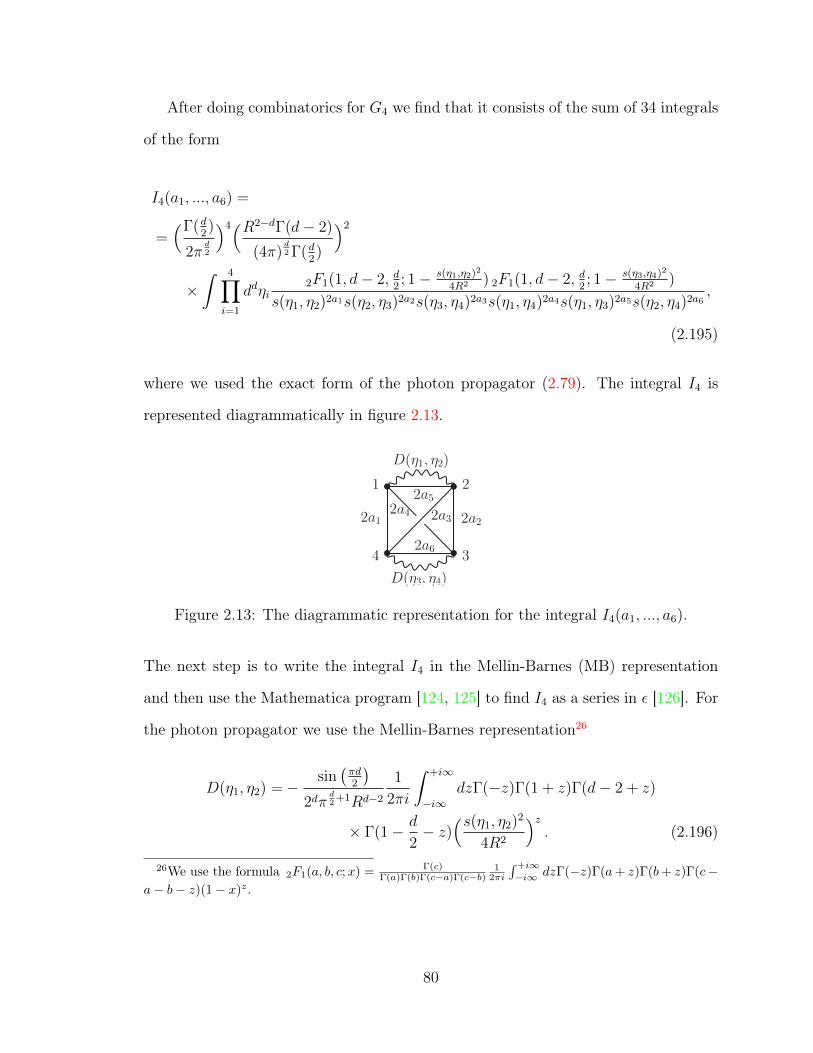
After doing combinatorics for G4 we find that it consists of the sum of 34 integrals

of the form

I4(a1, ..., a6) =

=(Γ(d

2)

2πd2

)4(R2−dΓ(d− 2)

(4π)d2 Γ(d

2)

)2

×∫ 4∏

i=1

ddηi2F1(1, d− 2, d

2; 1− s(η1,η2)2

4R2 ) 2F1(1, d− 2, d2; 1− s(η3,η4)2

4R2 )

s(η1, η2)2a1s(η2, η3)2a2s(η3, η4)2a3s(η1, η4)2a4s(η1, η3)2a5s(η2, η4)2a6,

(2.195)

where we used the exact form of the photon propagator (2.79). The integral I4 is

represented diagrammatically in figure 2.13.

2a1 2a2

2a5

2a6

2a4 2a3

1 2

34

D(η1, η2)

D(η3, η4)

Figure 2.13: The diagrammatic representation for the integral I4(a1, ..., a6).

The next step is to write the integral I4 in the Mellin-Barnes (MB) representation

and then use the Mathematica program [124, 125] to find I4 as a series in ε [126]. For

the photon propagator we use the Mellin-Barnes representation26

D(η1, η2) =− sin(πd2

)2dπ

d2

+1Rd−2

1

2πi

∫ +i∞

−i∞dzΓ(−z)Γ(1 + z)Γ(d− 2 + z)

× Γ(1− d

2− z)

(s(η1, η2)2

4R2

)z. (2.196)

26We use the formula 2F1(a, b, c;x) = Γ(c)Γ(a)Γ(b)Γ(c−a)Γ(c−b)

12πi

∫ +i∞−i∞ dzΓ(−z)Γ(a+ z)Γ(b+ z)Γ(c−

a− b− z)(1− x)z.

80

Then using methods similar as discussed in [54] one can write the general MB form

for the integral

I4(a1, ..., a6) =sin2(πd

2)Γ(d

2)4

2d+7π12

(5d+3)Γ(d+12

)(2R)2d+4−2

∑6i=1 ai

1

(2πi)5

∫ 5∏i=1

dziΓ(−z1)Γ(−z2)Γ(z1 + 1)

× Γ(z2 + 1)Γ(d− 2 + z1)Γ(1− d

2− z1)Γ(d− 2 + z2)Γ(1− d

2− z2)

× Γ2(d− a145 + z1, a1, a5 − z1|z3, z4, z5)

× Γ0(d− a235 + z1 − z4, d− a136 + z2 − z3, a3 − z5) , (2.197)

where amnk... ≡ am + an + ak + ... and Γ-blocks are

Γ0(a1, a2, b) =πd

Γ(d2)

Γ(d2− b)Γ(a1 + b− d

2)Γ(a2 + b− d

2)Γ(a1 + a2 + b− d)

Γ(a1)Γ(a2)Γ(a1 + a2 + 2b− d),

Γ2(a, b1, b2|z1, z2, z3) =

πd/23∏i=1

Γ(−zi)Γ(a+ b1 + b2 − d2

+∑3

i=1 zi)

Γ(a)Γ(b1)Γ(b2)Γ(d− a− b1 − b2)Γ(b1 + z1 + z3)

× Γ(b2 + z2 + z3)Γ(d− a− 2b1 − 2b2 − z1 − z2 − 2z3) . (2.198)

For some values of a1, ..., a6 the MB representation (2.197) is divergent or exactly

zero for any d (due to the term Γ(0)). To handle this problem we used an additional

regulator δ, so we were consistently calculating the integrals

Ireg4 (a1, ..., a6) = I4(a1 + δ, ..., a6 + δ) . (2.199)

Each integral out of 34 in G4 depends on δ and ε. But the G4 itself is free of δ and

depends only on ε as it should.

In general MB approach gives a result in terms of a series in ε and δ and each

coefficient of this series is a sum of convergent Melling-Barnes integrals, which are

independent of ε and δ and can be calculated numerically. The numerical result is

usually equal to some exact combinations of constants like π4, ζ(3), e.t.c. To get an

81

exact answer we used integer relation search algorithm PSLQ [127]. The final result

reads

G4 =N2f

6π4ε2+Nf

(8Nf (5 + 3(log(4πR2) + γ))− 18

)122π4ε

+1

123π4

(16N2

f

(5 + 3(log(4πR2) + γ)

)2

− 72Nf

(5 + 3(log(4πR2) + γ)

)+ 4(77 + 9π2)N2

f + 9Nf (72ζ(3)− 47)).

(2.200)

Note that in this calculation of G4 we have used d = 4− ε and N = Nf tr1 = 4Nf .

2.15 Appendix D. Calculation of ZT

In this appendix we present the computation of the ZT factor for the stress-energy

tensor in the theory of Critical QED. As we show below, a non-trivial ZT is required

for the Ward identity to hold. We define the “renormalized” stress-energy tensor T renµν

by

T renµν (x) = ZTTµν(x) , (2.201)

where ZT = 1 + (ZT1/∆ + Z ′T1)/N + O(1/N2), and Tµν is the “bare" stress-tensor.

To find ZT we will use the three-point function 〈T renµν (x1)Oren

m (x2)Orenm (x3)〉, where

Orenm = ZOmOm is the electron mass operator, ZOm is its renormalization constant

and the bare operator is

Om = ψψ . (2.202)

This three point function is gauge invariant. So using conformal invariance and

conservation of the stress-tensor, one has the general expression for the three-point

82

function

〈T renµν (x1)Oren

m (x2)Orenm (x3)〉 =

=−CTOmOm

(x212x

213)

d2−1(x2

23)∆Om−d2

+1

((X23)µ(X23)ν −

1

dδµν(X23)2

), (2.203)

where

(X23)ν =(x12)νx2

12

− (x13)νx2

13

. (2.204)

The conformal Ward identity gives

CTOmOm =1

Sd

d∆Om

d− 1COm , (2.205)

where COm and ∆Om are two-point constant and anomalous dimension of the operator

Om in coordinate space:

〈Orenm (x)Oren

m (0)〉 =COm

(x2)∆Om. (2.206)

Taking the Fourier transform of (2.203) and setting the momentum of the stress-

energy tensor to zero for simplicity, one finds in terms of the projected stress tensor

T = zµzνTµν

〈T ren(0)Orenm (p)Oren

m (−p)〉 = (d− 2∆Om)COmp2z

(p2)d2−∆Om+1

, (2.207)

where COm is the two-point constant of 〈Orenm Oren

m 〉 correlator in the momentum space:

〈Orenm (p)Oren

m (−p)〉 =COm

(p2)1− d2−ηm

, (2.208)

83

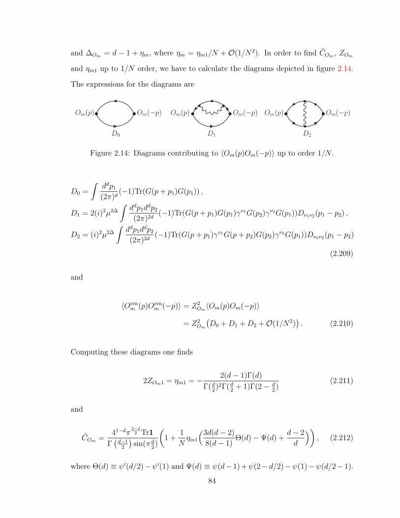
and ∆Om = d − 1 + ηm, where ηm = ηm1/N + O(1/N2). In order to find COm , ZOm

and ηm1 up to 1/N order, we have to calculate the diagrams depicted in figure 2.14.

The expressions for the diagrams are

Om(p) Om(−p)

D0 D2

Om(p) Om(−p)

D1

Om(p) Om(−p)

Figure 2.14: Diagrams contributing to 〈Om(p)Om(−p)〉 up to order 1/N .

D0 =

∫ddp1

(2π)d(−1)Tr(G(p+ p1)G(p1)) ,

D1 = 2(i)2µ2∆

∫ddp1d

dp2

(2π)2d(−1)Tr(G(p+ p1)G(p1)γν1G(p2)γν2G(p1))Dν1ν2(p1 − p2) ,

D2 = (i)2µ2∆

∫ddp1d

dp2

(2π)2d(−1)Tr(G(p+ p1)γν1G(p+ p2)G(p2)γν2G(p1))Dν1ν2(p1 − p2)

(2.209)

and

〈Orenm (p)Oren

m (−p)〉 = Z2Om〈Om(p)Om(−p)〉

= Z2Om

(D0 +D1 +D2 +O(1/N2)

). (2.210)

Computing these diagrams one finds

2ZOm1 = ηm1 = − 2(d− 1)Γ(d)

Γ(d2)2Γ(d

2+ 1)Γ(2− d

2)

(2.211)

and

COm =41−dπ

3−d2 Tr1

Γ(d−1

2

)sin(π d

2)

(1 +

1

Nηm1

(3d(d− 2)

8(d− 1)Θ(d)−Ψ(d) +

d− 2

d

)), (2.212)

where Θ(d) ≡ ψ′(d/2)−ψ′(1) and Ψ(d) ≡ ψ(d− 1) +ψ(2− d/2)−ψ(1)−ψ(d/2− 1).

84

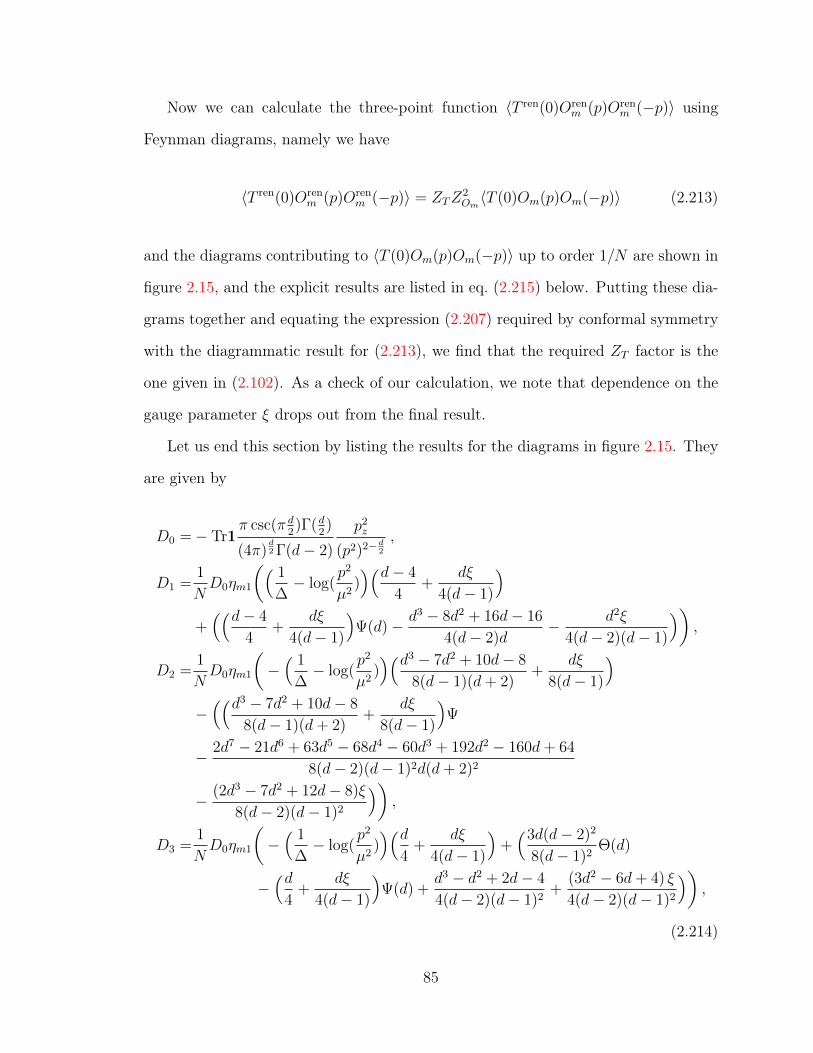
Now we can calculate the three-point function 〈T ren(0)Orenm (p)Oren

m (−p)〉 using

Feynman diagrams, namely we have

〈T ren(0)Orenm (p)Oren

m (−p)〉 = ZTZ2Om〈T (0)Om(p)Om(−p)〉 (2.213)

and the diagrams contributing to 〈T (0)Om(p)Om(−p)〉 up to order 1/N are shown in

figure 2.15, and the explicit results are listed in eq. (2.215) below. Putting these dia-

grams together and equating the expression (2.207) required by conformal symmetry

with the diagrammatic result for (2.213), we find that the required ZT factor is the

one given in (2.102). As a check of our calculation, we note that dependence on the

gauge parameter ξ drops out from the final result.

Let us end this section by listing the results for the diagrams in figure 2.15. They

are given by

D0 =− Tr1π csc(π d

2)Γ(d

2)

(4π)d2 Γ(d− 2)

p2z

(p2)2− d2

,

D1 =1

ND0ηm1

(( 1

∆− log(

p2

µ2))(d− 4

4+

dξ

4(d− 1)

)+((d− 4

4+

dξ

4(d− 1)

)Ψ(d)− d3 − 8d2 + 16d− 16

4(d− 2)d− d2ξ

4(d− 2)(d− 1)

)),

D2 =1

ND0ηm1

(−( 1

∆− log(

p2

µ2))(d3 − 7d2 + 10d− 8

8(d− 1)(d+ 2)+

dξ

8(d− 1)

)−((d3 − 7d2 + 10d− 8

8(d− 1)(d+ 2)+

dξ

8(d− 1)

)Ψ

− 2d7 − 21d6 + 63d5 − 68d4 − 60d3 + 192d2 − 160d+ 64

8(d− 2)(d− 1)2d(d+ 2)2

− (2d3 − 7d2 + 12d− 8)ξ

8(d− 2)(d− 1)2

)),

D3 =1

ND0ηm1

(−( 1

∆− log(

p2

µ2))(d

4+

dξ

4(d− 1)

)+(3d(d− 2)2

8(d− 1)2Θ(d)

−(d

4+

dξ

4(d− 1)

)Ψ(d) +

d3 − d2 + 2d− 4

4(d− 2)(d− 1)2+

(3d2 − 6d+ 4) ξ

4(d− 2)(d− 1)2

)),

(2.214)

85

D4 =1

ND0ηm1

(( 1

∆− log(

p2

µ2))(d− 4

8+

dξ

8(d− 1)

)+((d− 4

8+

dξ

8(d− 1)

)Ψ(d)

+3d3 − 16d2 + 32d− 16

8(d− 2)(d− 1)d− d2ξ

8(d− 2)(d− 1)2

)),

D5 =1

ND0ηm1

(−( 1

∆− 2 log(

p2

µ2))( (d− 2)2

4(d− 1)(d+ 2)

)−( (d− 2)2

2(d− 1)(d+ 2)Ψ(d)

− (d− 2) (5d4 − 9d3 + 4d2 + 28d− 16)

4(d− 1)2d(d+ 2)2− (d− 2)ξ

2(d− 1)2

)),

D6 =1

ND0ηm1

(3d(d− 2)

8(d− 1)2Θ(d) +

d− 2

4(d− 1)− (d− 2)ξ

2(d− 1)2

),

D7 =1

ND0ηm1

(3d(d− 2)

8(d− 1)2Θ(d) +

1

2(d− 1)− ξ

2(d− 1)

),

D8 =1

ND0ηm1

(( 1

∆− log(

p2

µ2))( d− 2

2(d− 1)

)+( (d− 2)

2(d− 1)Ψ(d)

− d2 − 3d+ 4

2(d− 1)d+

ξ

2(d− 1)

)),

D9 =1

ND0ηm1

(−( 1

∆− 2 log(

p2

µ2))( d− 2

4(d− 1)

)−( (d− 2)

2(d− 1)Ψ(d)

− d3 − 3d2 + 5d− 4

2(d− 1)2d+

(d− 2)ξ

2(d− 1)2

)),

D10 =1

ND0ηm1

(− 3d(d− 2)

8(d− 1)2Θ(d)− 2d− 3

2(d− 1)2+

(d− 2)ξ

2(d− 1)2

), (2.215)

where Θ(d) ≡ ψ′(d/2)−ψ′(1) and Ψ(d) ≡ ψ(d− 1) +ψ(2− d/2)−ψ(1)−ψ(d/2− 1)

and ηm1 is given in (2.211). We notice that

D7 +D8 +D9 +D10 =D0ηm1

N∆

(d− 2)

4(d− 1). (2.216)

86

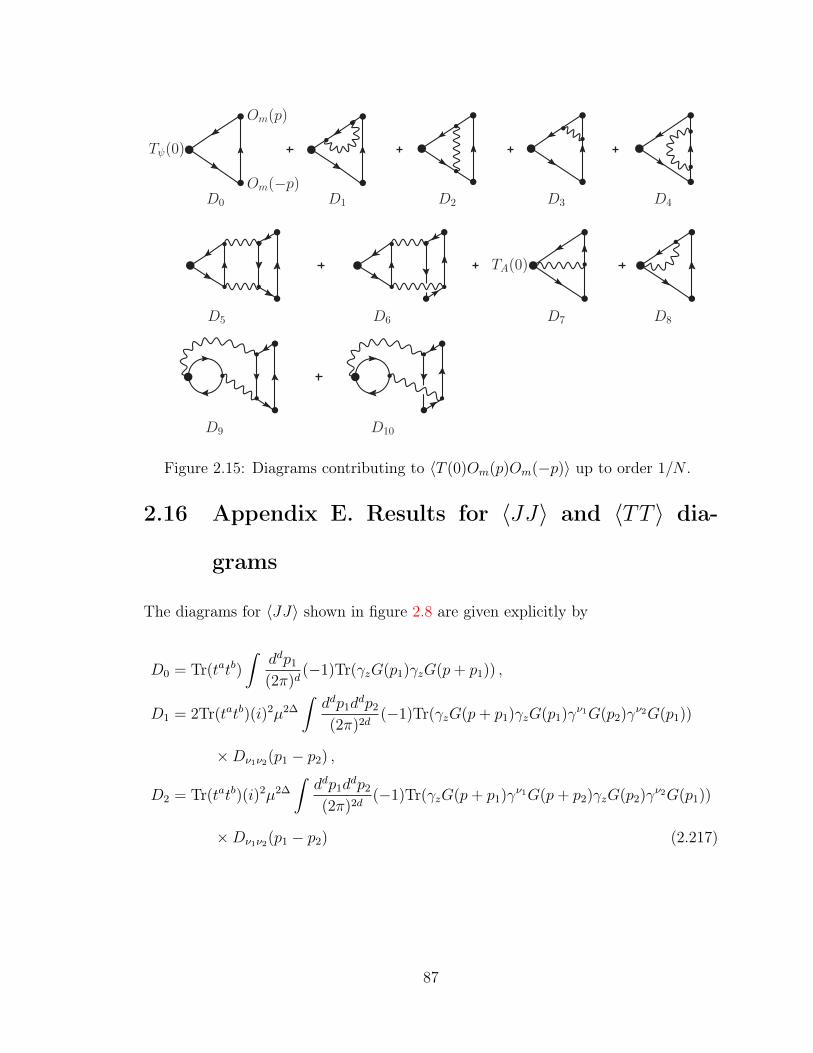
Tψ(0)

Om(p)

Om(−p)D0 D1 D2 D3 D4

TA(0)

D7 D8

D9 D10

D5 D6

Figure 2.15: Diagrams contributing to 〈T (0)Om(p)Om(−p)〉 up to order 1/N .

2.16 Appendix E. Results for 〈JJ〉 and 〈TT 〉 dia-

grams

The diagrams for 〈JJ〉 shown in figure 2.8 are given explicitly by

D0 = Tr(tatb)∫

ddp1

(2π)d(−1)Tr(γzG(p1)γzG(p+ p1)) ,

D1 = 2Tr(tatb)(i)2µ2∆

∫ddp1d

dp2

(2π)2d(−1)Tr(γzG(p+ p1)γzG(p1)γν1G(p2)γν2G(p1))

×Dν1ν2(p1 − p2) ,

D2 = Tr(tatb)(i)2µ2∆

∫ddp1d

dp2

(2π)2d(−1)Tr(γzG(p+ p1)γν1G(p+ p2)γzG(p2)γν2G(p1))

×Dν1ν2(p1 − p2) (2.217)

87

and the results are

D0 = Tr(tatb)Tr1π csc

(πd2

)Γ(d2

)(4π)

d2 (d− 1)Γ(d− 2)

p2z

(p2)2− d2

,

D1 =1

ND0ηm1

(( 1

∆− log(

p2

µ2))(d− 4

4+

dξ

4(d− 1)

)+((d− 4

4+

dξ

4(d− 1)

)Ψ(d)

+3d3 − 16d2 + 32d− 16

4(d− 2)(d− 1)d− d2ξ

4(d− 2)(d− 1)2

)),

D2 =1

ND0ηm1

(−( 1

∆− log(

p2

µ2))(d− 4

4+

dξ

4(d− 1)

)−((d− 4

4+

dξ

4(d− 1)

)Ψ(d)

− 3d(d− 2)

8(d− 1)Θ(d)− (d− 4)d

4(d− 2)(d− 1)− d2ξ

4(d− 2)(d− 1)2

)). (2.218)

The diagrams for 〈TT 〉 depicted in figure 2.10 are given explicitly by

D0 =Nf

(−i2

)2∫

ddp1

(2π)d(2p1z + pz)

2(−1)Tr(γzG(p+ p1)γzG(p1)),

D1 =2Nfµ2∆(−i

2

)2(i)2

∫ddp1d

dp2

(2π)2d(2p1z + pz)

2(−1)Tr(γzG(p+ p1)γzG(p1)γν1

×G(p2)γν2Gp1)Dν1ν2(p1 − p2) ,

D2 =Nfµ2∆(−i

2

)2(i)2

∫ddp1d

dp2

(2π)2d(2p1z + pz)(2p2z + pz)(−1)Tr(γzG(p+ p1)γν1

×G(p+ p2)γzG(p2)γν2Gp1)Dν1ν2(p1 − p2) ,

D3 =N2fµ

4∆(−i

2

)2(i)4

∫ddp1d

dp2ddp3

(2π)3d(2p1z + pz)(−1)Tr(γzG(p+ p1)γν1G(p1 − p3)

× γν2G(p1))Dν1ν3(p+ p3)Dν2ν4(p3)(2p2z + pz)

× (−1)Tr(γzG(p2)γν4G(p2 − p3)γν3G(p+ p2)) + . . . ,

(2.219)

88

D4 =2Nfµ2∆(−i

2

)(−i)(i)

∫ddp1d

dp2

(2π)2d(2p1z + pz)(−1)Tr(γzG(p+ p1)γzG(p2)

× γν1G(p1))Dν1z(p1 − p2) ,

D5 =2N2fµ

4∆(−i

2

)(−i)(i)3

∫ddp1d

dp2ddp3

(2π)3d(−1)Tr(γzG(p1 − p3)γν1G(p1))Dν1ν2(p3)

×Dzν3(p+ p3)(2p2z + pz)(−1)Tr(γzG(p2)γν2G(p2 − p3)γν3G(p+ p2)) + . . . ,

D6 =Nfµ2∆(−i)2

∫ddp1d

dp2

(2π)2d(−1)Tr(γzG(p+ p2)γzG(p1))Dzz(p1 − p2) ,

D7 =N2fµ

4∆(−i)2(i)2

∫ddp1d

dp2ddp3

(2π)3d(−1)Tr(γzG(p1 − p3)γν1G(p1))Dzz(p+ p3)

×Dν1ν2(p3)(−1)Tr(γzG(p2)γν2G(p2 − p3)) ,

D8 =N2fµ

4∆(−i)2(i)2

∫ddp1d

dp2ddp3

(2π)3d(−1)Tr(γzG(p1 − p3)γν1G(p1))Dν1z(p3)

×Dzν2(p+ p3)(−1)Tr(γzG(p2 − p3)γν2G(p+ p2)) , (2.220)

where dots mean that there is also an expression which corresponds to the opposite

direction of the fermion loop. After carrying out the momentum integrals using

techniques similar to the ones described in the appendices of [68], we find

D0 =−N π1− d2 csc(π d

2)Γ(d

2)

4d2

+1(d− 1)(d+ 1)Γ(d− 2)

p4z

(p2)2− d2

,

D1 =1

ND0ηm1

(( 1

∆− log(

p2

µ2))(d− 4

4+

dξ

4(d− 1)

)+((d− 4

4+

dξ

4(d− 1)

)Ψ(d)

+2d4 − 10d3 + 15d2 + 4d− 8

2(d− 2)(d− 1)d(d+ 1)− d(2d− 1)ξ

2(d− 2)(d− 1)2(d+ 1)

)),

D2 =1

ND0ηm1

(−( 1

∆− log(

p2

µ2))(d3 − 7d2 + 10d− 8

4(d− 1)(d+ 2)+

dξ

4(d− 1)

)+(3d(d− 2)

8(d− 1)Θ(d)−

(d3 − 7d2 + 10d− 8

4(d− 1)(d+ 2)+

dξ

4(d− 1)

)Ψ(d)

+5d5 − 27d4 + 44d3 − 30d2 − 12d+ 16

2(d− 2)(d− 1)2d(d+ 1)(d+ 2)− (d3 − 4d2 + 2) ξ

2(d− 2)(d− 1)2(d+ 1)

)),

D3 =1

ND0ηm1

(−( 1

∆− 2 log(

p2

µ2))( (d− 2)2

2(d− 1)(d+ 2)

)+( 2(d− 2)

(d− 1)(d+ 2)Ψ(d)

− d (d3 − 8d+ 11)

(d− 1)2(d+ 1)(d+ 2)+

ξ

2(d− 1)

))+ dD0/(2N) , (2.221)

89

and

D4 =1

ND0ηm1

(( 1

∆− log(

p2

µ2))(d− 2

d− 1

)+((d− 2)Ψ(d)

d− 1− d4 − 4d3 + 5d2 + 2d− 2

(d− 1)2d(d+ 1)+

ξ

d− 1

)),

D5 =1

ND0ηm1

(−( 1

∆− 2 log(

p2

µ2))( d− 2

2(d− 1)

)−((d− 2)Ψ(d)

d− 1

− d4 − 4d3 + 5d2 + 2d− 2

(d− 1)2d(d+ 1)+

ξ

d− 1

))− dD0/N ,

D6 =1

ND0ηm1

(− ξ − 1

2(d− 1)

),

D7 =1

ND0ηm1

(ξ − 1

2(d− 1)

),

D8 =dD0/(2N) , (2.222)

where Θ(d) ≡ ψ′(d/2)−ψ′(1) and Ψ(d) ≡ ψ(d− 1) +ψ(2− d/2)−ψ(1)−ψ(d/2− 1)

and ηm1 is given in (2.211). We notice that

D4 +D5 +D6 +D7 +D8 =D0ηm1

N∆

(d− 2)

2(d− 1)− dD0/(2N) . (2.223)

90

Chapter 3

Particle Production in 1 + 1 CFT

This chapter is an edited version of ref. [128] written in collaboration with Guilherme

Pimentel and Alexander Polyakov.

3.1 Introduction

In this chapter we discuss vacuum decay in 1 + 1 dimensional Conformal Field The-

ories with external fixed background fields. As an example, we consider a theory of

massless fermions in 1+1 dimensions coupled to Abelian, non-Abelian or gravitational

background fields. The computation of the vacuum decay rate involves evaluating the

effective action, which is given by the logarithm of the determinant of the quantum

fields in the fixed background. The pioneering example, due to Schwinger [129], is

of fermions in a constant background electric field. The example we study in our

paper is interesting, as we can find formulas for vacuum decay in generic field profiles

(which satisfy a few technical assumptions that we state below). Some exact results

for generic field profiles were also obtained in [130, 131], in 1 + 1 dimensional QED.

Let us briefly review a case with no particle production. Consider free massless

fermions interacting with a fixed non-Abelian gauge field background. The effective

action is obtained by the Gaussian integration over the fermion fields, and is given

91

by a one loop determinant. If the field profile satisfies a “good" behavior, that we

specify later, the effective action is real and is expressed [132] in terms of the Wess-

Zumino-Novikov-Witten (WZNW) action [133, 134, 135]. In this case particles are

not created, since the vacuum decay rate is nonzero only when the effective action

has an imaginary part.

Our goal is to determine the effective action for background fields that do lead

to particle production. In this case, we have to discuss the in/out effective action

which has an imaginary part, reflecting vacuum decay. The imaginary piece in the

effective action is determined by a careful treatment of the Feynman iε prescription

in a massless theory.

Our main result is that the effective action is modified by the inclusion of extra

boundary terms, which are complex, and whose imaginary part gives the vacuum

decay rate. The boundary term is a two-form which appears to be novel. To compute

the boundary terms we need a certain Riemann-Hilbert decomposition. While the

Abelian and non-Abelian decompositions are standard Riemann-Hilbert problems,

the gravitational case has not been considered before. The vacuum decay rate for

Abelian background fields is given by the same formula of dissipative quantum me-

chanics obtained by Caldeira and Leggett [136, 137]. Our results generalize their

formulas for non-Abelian and gravitational backgrounds.

The rest of the chapter is organized as follows. In section 3.2 we compute the

effective action and the new boundary term for an Abelian gauge field and discuss

the general logic of the computation, which helps in the more complicated cases. In

section 3.3 we find the effective action and the new boundary term for the non-Abelian

gauge field. Finally, in section 3.4 we find the effective action and the new boundary

term in the case of the gravitational field. In appendix 3.5, we discuss an alternative

method of computation of the boundary terms. In appendix 3.6, we review the

gauge-gravity duality between the non-Abelian and gravitational cases [138, 139, 140].

92

Finally, in appendix 3.7, we show the first perturbative correction to the Caldeira-

Leggett formula coming from non-Abelian and gravitational backgrounds.

3.2 Vacuum decay in an Abelian background

To set the stage, let us look at the Abelian case first. The Lagrangian is

L = ψγµ(i∂µ + Aµ)ψ = ψ−(i∂+ + A+)ψ− + ψ+(i∂− + A−)ψ+, (3.1)

where the metric is ηµν = (1,−1), and we introduced light cone coordinates x± =

(x0±x1)/√

2. From the Lagrangian it is clear that the left movers ψ+ and right movers

ψ− are sourced by A− and A+ fields, respectively. Therefore, the determinant will

split into a right-moving piece, a left-moving piece, and a contact term that ensures

gauge invariance [132]1

S(A+, A−) = log det(γµ(i∂µ + Aµ)) = W+(A+) +W−(A−)− 2

∫d2xA+A− . (3.2)

The contact term comes from short distance cutoff regulators; it is not related to

particle production. In the case of strong fields which lead to particle production,

W+ and W− have imaginary parts. The vacuum decay rate factorizes and is given by

|out〈0|0〉in|2 = e−2ImS(A) = e−2ImW+e−2ImW− . (3.3)

Let us compute the contribution to the effective action coming from A+. We will treat

x+ as a time coordinate, while in the x− direction we assume that A+(x+, x−) → 0

as x− → ±∞. An easy calculation of the diagram

1In this section we write the effective action up to an unimportant overall factor − e2

4π . In otherwords, we set e2 = −4π. The charge e can be restored by the substitution Aµ → eAµ.

93

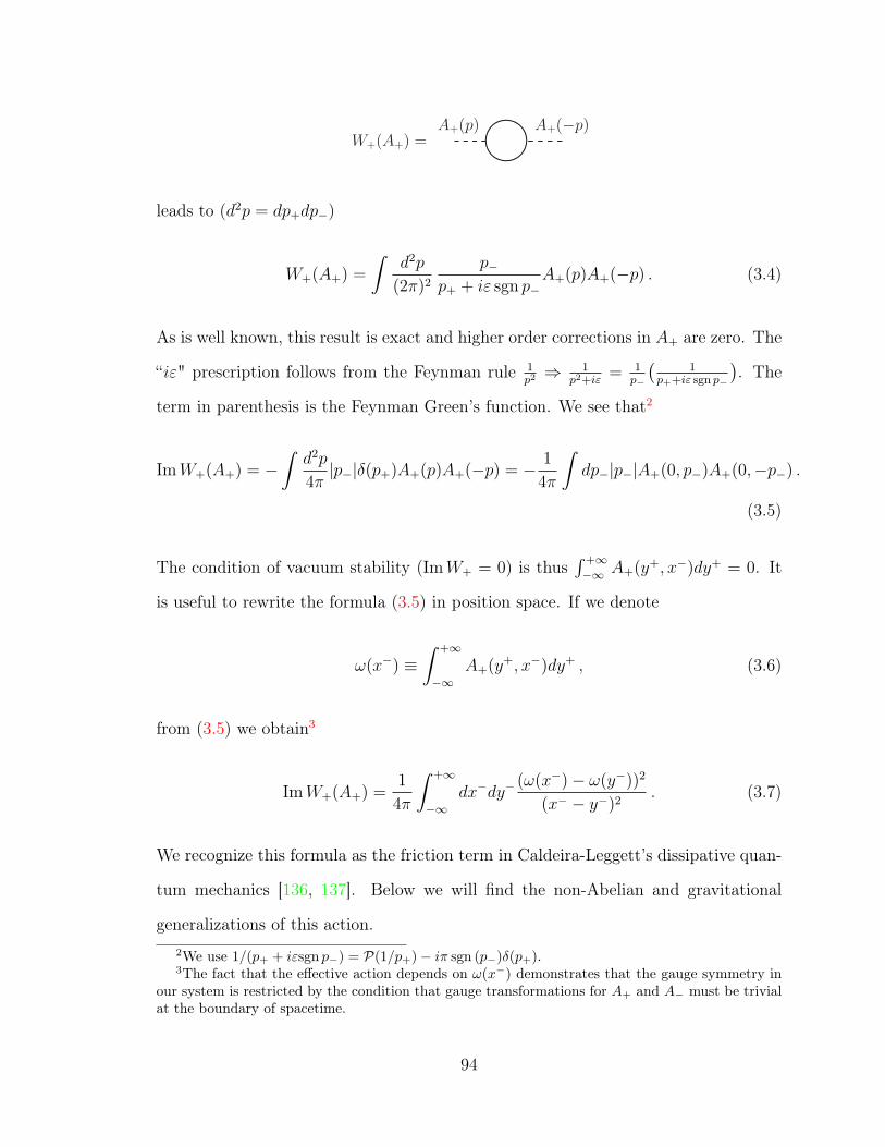
W+(A+) =A+(p) A+(−p)

leads to (d2p = dp+dp−)

W+(A+) =

∫d2p

(2π)2

p−p+ + iε sgn p−

A+(p)A+(−p) . (3.4)

As is well known, this result is exact and higher order corrections in A+ are zero. The

“iε" prescription follows from the Feynman rule 1p2 ⇒ 1

p2+iε= 1

p−

(1

p++iε sgn p−

). The

term in parenthesis is the Feynman Green’s function. We see that2

ImW+(A+) = −∫d2p

4π|p−|δ(p+)A+(p)A+(−p) = − 1

4π

∫dp−|p−|A+(0, p−)A+(0,−p−) .

(3.5)

The condition of vacuum stability (ImW+ = 0) is thus∫ +∞−∞ A+(y+, x−)dy+ = 0. It

is useful to rewrite the formula (3.5) in position space. If we denote

ω(x−) ≡∫ +∞

−∞A+(y+, x−)dy+ , (3.6)

from (3.5) we obtain3

ImW+(A+) =1

4π

∫ +∞

−∞dx−dy−

(ω(x−)− ω(y−))2

(x− − y−)2. (3.7)

We recognize this formula as the friction term in Caldeira-Leggett’s dissipative quan-

tum mechanics [136, 137]. Below we will find the non-Abelian and gravitational

generalizations of this action.2We use 1/(p+ + iεsgn p−) = P(1/p+)− iπ sgn (p−)δ(p+).3The fact that the effective action depends on ω(x−) demonstrates that the gauge symmetry in

our system is restricted by the condition that gauge transformations for A+ and A− must be trivialat the boundary of spacetime.

94

It is instructive to rewrite (3.7) in a slightly different form. Let us introduce two

complex functions ωup(x−) and ωdown(x−), which are analytic in the upper and lower

half-planes, respectively. They are related to ω(x−) as

ωup(x−)− ωdown(x−) = ω(x−) (3.8)

for real x−. This decomposition of the function ω(x−) is called the scalar Riemann-

Hilbert problem and the explicit solution in this case is given by

ωup/down(x−) =1

2πi

∫ +∞

−∞

ω(y−)dy−

y− − x− ∓ iε . (3.9)

In terms of ωup/down, the imaginary part of the effective action can be written as

ImW+(A+) = Im∫ +∞

−∞dx− (ωdown∂−ωup) . (3.10)

The generalization of the formula (3.10) for the strong non-Abelian and gravitational

cases is the main goal of this paper.

There is yet another way of obtaining (3.10), which will be useful below. We can

parametrize A+ as

A+(x+, x−) = ∂+φ(x+, x−) (3.11)

and we notice that the “Wilson line" φ(x+, x−) has residual gauge invariance φ →

φ+ u(x−). We say that φ = φR(x+, x−) is in retarded gauge if it obeys the boundary

condition φR(−∞, x−)→ 0 and therefore

φR(x+, x−) =

∫ x+

−∞A+(y+, x−)dy+ . (3.12)

95

We see that φR is manifestly real and causal, as φR(x+, x−) only depends on

A+(y+, x−) for y+ < x+; moreover, φR(+∞, x−) = ω(x−), so the imaginary part of

the effective action (3.10) is written in terms of the boundary value of φR and the

whole W+(A+) reads

W+(A+) =

∫d2x ∂+φR∂−φR +

∫ +∞

−∞dx− (ωdown∂−ωup) . (3.13)

We can use the solution of the Riemann-Hilbert problem (3.8) and the residual gauge

invariance of φ to define a spectral (or Feynman) gauge, namely

φS(x+, x−) ≡ φR(x+, x−)− ωdown(x−)→

ωup(x−), x+ → +∞

−ωdown(x−), x+ → −∞. (3.14)

In the spectral gauge the effective action (3.13) reads

W+(A+) =

∫d2x ∂+φS∂−φS , (3.15)

and has the form of the usual result [12]. In our case, the difference is that the function

φS is complex valued and (3.15) contains both real and imaginary parts of the effective

action! The conclusion is that in the spectral gauge, we do not require boundary terms

in the effective action, whereas in the retarded gauge, we have boundary terms, which

are complex and account for the vacuum decay.

The logic is summarized as follows. If we use the spectral gauge, then the expres-

sions for the effective actions are well known [12, 132, 141], as the boundary terms

evaluate to zero. Then passing from the spectral gauge to retarded gauge we determine

the functional form of the boundary terms. In the retarded gauge, the boundary term

contains the imaginary part of the effective action. In Appendix 3.5 we discuss an

96

alternative method to compute the full effective action, by exploiting (chiral or trace)

anomaly equations.

3.3 Vacuum decay in a non-Abelian background

In the non-Abelian case the general form of the effective action reads

S(A+, A−) = log det(γµ(i∂µ + Aµ)) = W+(A+) +W−(A−) + 2

∫d2xTr(A+A−)

(3.16)

and imaginary terms responsible for the particle production are present only in W+

and W−. We concentrate again on W+(A+), which is formally given by the following

sum of Feynman diagrams

W+(A+) =

If we parametrize A+ = g−1∂+g we get W+(g). If g(x+ → ±∞, x−) = 1 then W+(g)

is the WZNW action [142]

WWZNW(g) ≡ 1

2

∫d2xTr(∂µg−1∂µg)− 1

3

∫d2xdt εµνλTr(g−1∂µgg

−1∂νgg−1∂λg) ,

(3.17)

where in the last Wess-Zumino (WZ) term we introduced the extra t-dependence:

g(x+, x−, t) such that g(x+, x−, 0) = 1 and g(x+, x−, 1) = g(x+, x−); and µ, ν, λ =

(±, 0), and ε0−+ = 1, where zero corresponds to the t coordinate.

97

From the Abelian case, we expect that vacuum decay occurs for A+ with

g−1(−∞, x−) ·g(+∞, x−) 6= 1, or, in different notation:

Ω(x−) ≡ P exp

∫ ∞−∞

A+(y+, x−)dy+ 6= 1, (3.18)

where “P exp" is the path-ordered exponential. In this case the effective action is not

given by (3.17); it must include new boundary terms. Indeed, looking at the variation

of the WZ term

SWZ ≡∫d2xdt εµνλTr(aµaνaλ) , (3.19)

where aµ ≡ g−1∂µg, with δaµ = ∇µε, we obtain

δSWZ =

∫d2xdt εµνλTr(aµaν∇λε) ∼

∫d2xdt εµνλ∇λTr

((∂µaν − ∂νaµ)ε

)=

∫d2xdt εij ∂0Tr(∂iajε)−

∫d2xdt ∂+Tr

((∂−a0 − ∂0a−)ε

)=

∫d2x εijTr(∂iajε)−

∫dx−dt Tr

((∂−a0 − ∂0a−)ε

)∣∣x+=+∞x+=−∞ . (3.20)

The first term here is standard while the time-boundary term explicitly violates t-

symmetry. In other words, SWZ is dependent on the t-parametrization. This unphys-

ical dependence on the extrapolation disappears when the right boundary terms are

added to WZNW action.

Notice that the matrix g has a gauge symmetry

g(x+, x−)→ u(x−)g(x+, x−) , (3.21)

where u(x−) is an arbitrary complex matrix. The retarded gauge is defined by

gR(x+ → −∞, x−) = 1 ⇒ gR(x+, x−) = P exp

∫ x+

−∞dy+A+(y+, x−) . (3.22)

98

Like in the Abelian case, we see that Ω(x−) = gR(+∞, x−).

Proceeding by analogy, we should look for complex valued matrices Ωdown(x−) and

Ωup(x−) that are a solution to the matrix Riemann-Hilbert problem

Ωdown(x−)Ωup(x−) = Ω(x−) , (3.23)

for real values of x−. We assume that Ω−1up (x−) and Ω−1

down(x−) are also analytic in the

upper and lower half-planes, respectively. Unfortunately, the matrix Riemann-Hilbert

problem does not have an explicit general solution.4

As we see from (3.20) the retarded gauge choice requires extra terms in the WZ

term in order to cancel the unacceptable boundary contributions. However, we can use

our gauge freedom in choosing g to eliminate the boundary terms. Let us introduce

the spectral (or Feynman) gauge:

gS(x+, x−) ≡ Ω−1down(x−) gR(x+, x−)→

Ωup(x−), x+ → +∞

Ω−1down(x−), x+ → −∞

. (3.24)

It follows from here that gS(x+, x−) at x+ → ±∞ is analytic in the lower/upper

half-planes and thus all boundary terms vanish after x− integration. By analogy with

the Abelian case, we come to the conclusion that in the spectral gauge there are

no boundary terms! The effective action is just the standard WZNW action (3.17),

which is complex valued, as gS is complex

W+(A+) = WWZNW(gS) . (3.25)

4For a review on the subject and the cases where an explicit solution is available, see [143].Notice that the right and left decompositions are inequivalent, namely, we could look for Ω(x−) =

Ωup(x−)Ωdown(x−), but in terms of these matrices we do not obtain spectral boundary conditionsin a simple way. In general Ωup/down(x−) 6= Ωup/down(x−).

99

A more physical justification of the absence of boundary terms in the spectral gauge

is discussed in the Appendix 3.5.

From (3.25), we now determine the boundary term that must be present in the

effective action written in an arbitrary gauge. For example, in going from spectral to

retarded gauge, we do not change A+ = g−1∂+g, therefore the effective actions must

be the same,

W+(A+) = WWZNW(Ω−1downgR) = WWZNW(gR) +WB(Ωup,Ωdown) . (3.26)

In order to proceed we use exterior calculus to derive a composition formula for

the WZ term. Let us introduce two 1-forms a and b, with a = g−1dg, b = dhh−1 .

a and b satisfy the equations da = −a ∧ a, db = b ∧ b . Consider the 1-form c =

(gh)−1d(gh) = h−1(a+ b)h. Then we have

Tr(c ∧ c ∧ c) = Tr(a ∧ a ∧ a) + Tr(b ∧ b ∧ b)− 3d(Tr a ∧ b) . (3.27)

Now we apply (3.27) with gS = Ω−1downgR. From the quadratic term in the WZNW

action we obtain5

1

2

∫d2xTr(∂µg−1

S ∂µgS) =1

2

∫d2xTr(∂µg−1

R ∂µgR) +

∫d2xTr(∂−ΩdownΩ−1

down∂+gRg−1R ) ,

(3.28)

and using (3.26) and (3.27) for the WZ term in (3.17) we find

WWZ(gS) = WWZ(gR)− 3

∫(x+,x−,t)

d(Tr(ΩdowndΩ−1

down ∧ dgRg−1R )). (3.29)

Notice that the Penrose diagram for our space-time with the embedding dimension is

a pyramid; we call it the Penrose-Nefertiti diagram (see figure 3.1).5In light-cone coordinates Tr(∂µg−1∂µg) = Tr(∂−g−1∂+g) + Tr(∂+g

−1∂−g) = 2Tr(∂+g−1∂−g).

100

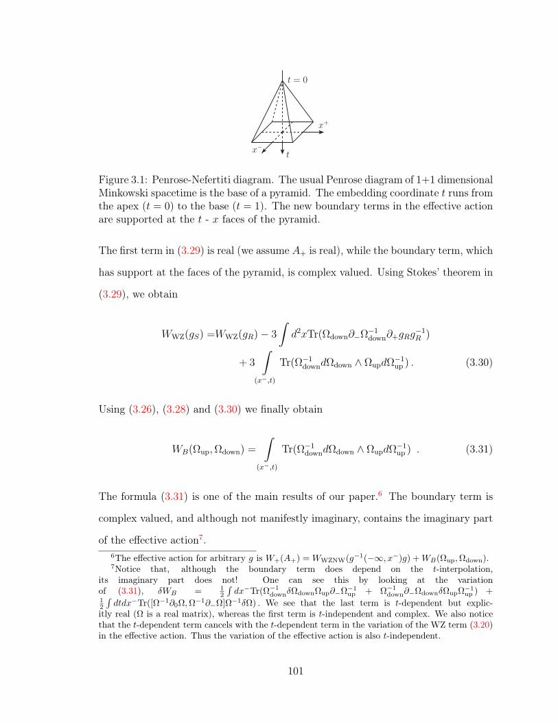
x+

x−t

t = 0

Figure 3.1: Penrose-Nefertiti diagram. The usual Penrose diagram of 1+1 dimensionalMinkowski spacetime is the base of a pyramid. The embedding coordinate t runs fromthe apex (t = 0) to the base (t = 1). The new boundary terms in the effective actionare supported at the t - x faces of the pyramid.

The first term in (3.29) is real (we assume A+ is real), while the boundary term, which

has support at the faces of the pyramid, is complex valued. Using Stokes’ theorem in

(3.29), we obtain

WWZ(gS) =WWZ(gR)− 3

∫d2xTr(Ωdown∂−Ω−1

down∂+gRg−1R )

+ 3

∫(x−,t)

Tr(Ω−1downdΩdown ∧ ΩupdΩ−1

up ) . (3.30)

Using (3.26), (3.28) and (3.30) we finally obtain

WB(Ωup,Ωdown) =

∫(x−,t)

Tr(Ω−1downdΩdown ∧ ΩupdΩ−1

up ) . (3.31)

The formula (3.31) is one of the main results of our paper.6 The boundary term is

complex valued, and although not manifestly imaginary, contains the imaginary part

of the effective action7.6The effective action for arbitrary g is W+(A+) = WWZNW(g−1(−∞, x−)g) +WB(Ωup,Ωdown).7Notice that, although the boundary term does depend on the t-interpolation,

its imaginary part does not! One can see this by looking at the variationof (3.31), δWB = 1

2

∫dx−Tr(Ω−1

downδΩdownΩup∂−Ω−1up + Ω−1

down∂−ΩdownδΩupΩ−1up ) +

12

∫dtdx−Tr([Ω−1∂0Ω,Ω−1∂−Ω]Ω−1δΩ) . We see that the last term is t-dependent but explic-

itly real (Ω is a real matrix), whereas the first term is t-independent and complex. We also noticethat the t-dependent term cancels with the t-dependent term in the variation of the WZ term (3.20)in the effective action. Thus the variation of the effective action is also t-independent.

101

We emphasize that this boundary term is the non-Abelian generalization of the

Caldeira-Leggett dissipative term, and is given by a two-form8. We also notice

that our two-form is a Minkowski space counterpart of the Atiyah-Patodi-Singer η-

invariant [146, 147, 148], which appears in Euclidean manifolds with boundary. We

present the leading order, non-Abelian correction to the Caldeira-Leggett formula in

Appendix 3.7.

3.4 Vacuum decay in the gravitational field

Now we consider a theory of fermions coupled to a fixed gravitational field. It is

convenient to parametrize the metric in the light cone coordinates,

ds2 = h+−(x+, x−)dx+dx− + h++(x+, x−)dx+dx+ + h−−(x+, x−)dx−dx− . (3.32)

We assume that the background fields are asymptotically flat, i.e. h++(x+, x−)→ 0,

h−−(x+, x−)→ 0 and h+−(x+, x−)→ 1 as x± → ±∞. The Lagrangian is9

L = ψ−(∂+ − h++∂−)ψ− + ψ+(∂− − h−−∂+)ψ+ . (3.33)

Like in the non-Abelian case, the effective action is

S(h++, h−−, h+−) = W+(h++) +W−(h−−) + L(h++, h−−, h+−) , (3.34)

where the last term L is a local and real term and appears due to the UV regulator.

We concentrate on the calculation of the contribution from left-moving fermions,

W+(h++). For gravity we use the same logic as in the non-Abelian case. We8A similar two-form was found in Euclidean manifolds with a boundary, in [144, 145].9For simplicity, we consider Majorana fermions. As in [149], we perform a field redefinition to

write the Lagrangian in the form (3.33). In the previous sections, we considered Dirac fermions, asthese can carry electric and color charge.

102

parametrize the metric tensor h++(x+, x−) using the function f(x+, x−) defined by

the equation

(∂+ − h++∂−)f = 0 , (3.35)

which is a gravitational analog of the Wilson line. Lines of constant f correspond to

the characteristics of light-like, right-moving geodesics in the background spacetime.

Notice that there is an ambiguity in f , namely

f(x+, x−) ⇒ u(f(x+, x−)) , (3.36)

where u(x−) is an arbitrary invertible complex function of one variable. The retarded

gauge is defined by

fR(x+ → −∞, x−) = x− ⇒ fR(x+, x−) ≡ P exp(∫ x+

−∞dy+h++(y+, x−)∂−

)x− .

(3.37)

As in the case of gauge fields, we need to add a suitable boundary term to the effective

action [141]

WgWZ(f) ≡∫

d2x

(∂2−f∂+∂−f

(∂−f)2− (∂2

−f)2∂+f

(∂−f)3

), (3.38)

where gWZ stands for “gravitational Wess-Zumino" and we omit an overall normal-

ization factor, which is −1/48π in our case. Alternatively, we can use the gauge

symmetry (3.36) to eliminate the boundary term. Let us introduce the spectral gauge

by

fS(x+, x−) ≡ Γ−1down(fR(x+, x−)) =

Γup(x−), x+ → +∞ ,

Γ−1down(x−), x+ → −∞ ,

(3.39)

103

where Γup(x−) and Γdown(x−) are analytic functions in the upper and lower x− half-

plane. We also assume that the inverse functions Γ−1up (x−) and Γ−1

down(x−) are analytic

in the upper and lower x− half-plane respectively. In this case, to determine Γup,down,

we need to solve a “functional” Riemann-Hilbert problem 10,

Γdown(Γup(x−)) = Γ(x−) , (3.40)

where

Γ(x−) ≡ P exp(∫ +∞

−∞dy+h++(y+, x−)∂−

)x− = fR(+∞, x−) . (3.41)

To our knowledge, the Riemann-Hilbert problem (3.40) has not been considered in

the mathematics literature before. We also notice that (3.40) doesn’t have an explicit

solution. 11

By similar arguments as in the previous sections, the effective action is

W+(h++) = WgWZ(fS) , (3.42)

where WgWZ is given by (3.38). See also Appendix 3.5 for a different derivation of

(3.42). This effective action is complex valued. In retarded and spectral gauges the

metric h++(x+, x−) is the same, therefore we have the equality

W+(h++) = WgWZ(Γ−1down(fR)) = WgWZ(fR) +WB(Γup,Γdown) . (3.43)

10In an analogous fashion to the matrix Riemann-Hilbert problem, we can have right andleft decompositions of the function f . Namely, we can consider functions Γup/down such thatΓup(Γdown(x−)) = Γ(x−) in the real line. In general, Γup/down 6= Γup/down.

11Finding a physically relevant explicit solution to (3.40) seems to be hard. On the other hand onecan find solutions in terms of meromorphic funtions. For example, Γdown(x) = ε

1−x23

(x−a)2

(x−ix1)(x−ix2) ,Γup(x) = ax−b

x+ix3and Γ(x) = ε

1+x2 is a solution to (3.40), where a = i2 (x1 + x2 + (x1 − x2)x3),

b = 12 (x1 − x2 + (x1 + x2)x3), x1, x2, x3 > 0 and ε is an arbitrary real parameter.

104

Using (3.38), (3.43) we get

WB(Γup,Γdown) =

∫d2x ∂−fR

(Γ−1down)′′

(Γ−1down)′

∂−

(∂+fR∂−fR

). (3.44)

Now, introducing new variables y− = fR(x+, x−), y+ = x+ one can get12

WB(Γup,Γdown) =

∫dy−

∂

∂y−log((Γ−1

down)′(y−))

log(Γ′(Γ−1(y−))

). (3.45)

Finally introducing a coordinate s = Γ−1(y−) and using that (Γ−1down)′(Γ(s)) =

1/Γ′down(Γup(s)) and Γ′(s) = Γ′down(Γup(s))Γ′up(s) we obtain13

WB(Γup,Γdown) =

∫ds log

(Γ′down(Γup(s))

) ∂∂s

log(Γ′up(s)

). (3.46)

Therefore the effective action in the retarded gauge is

W+(h++) =

∫d2x

(∂2−fR∂+−fR(∂−fR)2

− (∂2−fR)2∂+fR(∂−fR)3

)+

∫ds log

(Γ′down(Γup(s))

) ∂∂s

log(Γ′up(s)

). (3.47)

The bulk term is manifestly real, while the boundary term is complex, and, in par-

ticular, contains the imaginary piece of the effective action.

In appendix 3.6, we review a connection between gauge theory and gravity in two

dimensions [138, 139, 140], and phrase (3.40) in terms of a matrix Riemann-Hilbert

problem, in the hope that this simple connection might be useful in finding explicit

solutions of the functional Riemann-Hilbert problem.12To arrive at this formula we need two steps. At step 1 we define the inverse function f−1

R (·, ·)by f−1

R (x+, fR(x+, x−)) = x− and notice that∫d2x∂−fR =

∫d2y and ∂− = (∂−fR)∂/∂y− =

(∂f−1R /∂y−)−1∂/∂y− and ∂+fR/∂−fR = −∂f−1

R /∂y+. At step 2 we integrate over y+ and use that∂f−1

R /∂y−(+∞, y−) = 1/Γ′(Γ−1(y−)) and ∂f−1R /∂y−(−∞, y−) = 1. It was crucial here to assume

that fR(x+, x−) is invertible for all x+.13The expression (3.45) is very similar to formula (5.23) in [150]. The reason for the similarity of

the results is puzzling to us and is an interesting open question.

105

3.5 Appendix A. Boundary conditions on induced

currents and alternative derivation of the bound-

ary actions

In this appendix we derive the effective action for non-Abelian and gravitational

cases using the anomaly equations. We start with the non-Abelian case. We define

Jµ ≡ δW/δAµ; then the anomaly equations read [142]14

∂µJ

µ + [Aµ, Jµ] = 0 ,

εµν(∂µJν + [Aµ, Jν ]) = εµνFµν .

(3.48)

Working in the light-cone cone coordinates x± and choosing the axial gauge A− = 0,

we get ∂−(A+ − J+) = 0 and (ε−+ = 1)

∂−A+ + ∂+J− − [J−, A+] = 0. (3.49)

Parametrizing A+ = g−1∂+g one can find that the general solution of (3.49) is

J− = −g−1∂−g − g−1j−g , (3.50)

where j− = j−(x−) is, at this stage, an arbitrary complex matrix function, which

depends only on x−, and has to be fixed by additional physical arguments. On the

other hand the variation of the effective action is

δW (A+) =

∫d2xTr(J−δA+) . (3.51)

14To restore the unimportant overall factor in front of the effective action one needs to replaceεµνFµν → εµν

2π Fµν .

106

As we will see below, it is exactly the term g−1j−g in the current J− which is respon-

sible for the imaginary part of the effective action.

In order to fix j−(x−) we use the “analyticity" argument. Namely we say that

the induced current out〈J−(x+, x−)〉in must satisfy the analytical (spectral) boundary

conditions15:

out〈J−(x+, x−)〉in →

Jup(x−), x+ → +∞ ,

Jdown(x−), x+ → −∞ ,

(3.52)

where Jup(x−) and Jdown(x−) are complex matrix functions analytic in the upper and

lower x− half-planes correspondingly16.

Now we return to determining j− in the expression for the induced current. Work-

ing in the retarded gauge gR(x+, x−) ≡ P exp∫ x+

−∞ dy+A+(y+, x−) and using (3.52)

one finds

j−R(x−) = −∂−ΩdownΩ−1down , (3.53)

where Ωdown and Ωup are matrices analtyic in the lower and upper half-planes, and

solve the matrix Riemann-Hilbert problem

Ωdown(x−)Ωup(x−) = P exp

∫ +∞

−∞dy+A+(y+, x−) . (3.54)

Correspondingly we find Jup(x−) = −Ω−1up ∂−Ωup and Jdown(x−) = ∂−ΩdownΩ−1

down.

15Although J−(x+, x−) is a hermitian operator, the matrix element out〈J−(x+, x−)〉in can becomplex valued, as we are not computing an expectation value of the current for a given state, butrather evaluating a transition amplitude between states without particles in the past and withoutparticles in the future.

16We can justify (3.52) as follows. First, we checked (3.52) diagramatically in perturbation theory,to third order in the background field. The other general argument invokes consideration of thecorrelation function out〈0|ψ+(y+, y−)ψ+(x+, x−)|0〉in , where x+ → −∞. In this limit ψ+(x+, x−)

is a free field and we have ψ+(−∞, x−) =∑p>0(ape

ipx− + a†pe−ipx−) . As ap|0〉in = 0 we see that

only e−ipx−

modes survive. These modes define an analytic function in x− in the lower half planebecause e−ipx

−decays when p > 0 and Imx− < 0. This argument can be applied for any operator

O(ψ+), to show that a correlation function 〈...O(−∞, x−)〉 is analytic in x− in the lower half-plane.

107

Notice that in the spectral gauge (3.24) we have j−S(x−) = 0. From this it follows

that, in the spectral gauge, the effective action is the WZNW action (3.25), evaluated

at gS, and there are no boundary terms. Now, as we determined the current

J− = −g−1R ∂−gR − g−1

R j−RgR , (3.55)

one can check that the variation of W+(A+) (see (3.17) and (3.31)) indeed equals to

(3.51).

In the gravitational case everything is similar to the non-Abelian case. In the

light-cone coordinates and the axial gauge h−− = 0, the anomaly equation reads

[141]17

(∂+ − h++∂− − 2(∂−h++))T−− = −2∂3−h++ . (3.56)

Parametrizing h++ by f(x+, x−), with (∂+ − h++∂−)f = 0, the general solution of

the equation (3.56) is

T−−(x+, x−) = −2D−f + (∂−f)2t−(f) , (3.57)

where we define the Schwarzian

D−f ≡∂3−f

∂−f− 3

2

(∂2−f)2

(∂−f)2(3.58)

and t−(f) is at this stage is an arbitrary complex function, which has to be fixed by

additional physical arguments18. So analogously to the non-Abelian case we say that

the induced current out〈T−−(x+, x−)〉in must satisfy the analytical (spectral) boundary17To restore the overall factor in front of the effective action one needs to replace −2∂3

−h++ →1

24π∂3−h++.

18The logic is very similar to that of the paper [151], where the term t−(f) in the stress-energytensor is fixed by choosing a particular state.

108

conditions:

out〈T−−(x+, x−)〉in →

Tup(x−), x+ → +∞ ,

Tdown(x−), x+ → −∞ ,

(3.59)

where Tup(x−) and Tdown(x−) are some complex functions analytic in the upper and

lower x− half-planes correspondingly. Again, working in the retarded gauge, defined

by the condition fR(x+ → −∞, x−) = x− we find that19

t−R(f) = −2DfΓ−1down(f) , (3.60)

where Γup(x−) and Γdown(x−) are invertible, analytic functions in the upper and lower

x− half-plane, and they are solutions of the functional Riemann-Hilbert problem

(Γ(x−) ≡ fR(+∞, x−))

Γdown(Γup(x−)) = Γ(x−) . (3.61)

We have Tup(x−) = −2D−Γup and Tdown(x−) = −2D−Γ−1down and we again notice that

t−S(f) = 0 in the spectral gauge fS, defined in (3.39), which leads to the formula

(3.42).

Having the expression for the current T−− = −2D−Γ−1down(fR), we can check that

the variation of (3.47) is indeed equal to

δW (h++) =

∫d2xT−−δh++ . (3.62)

19It is convenient here to use the composition formula for the Schwarzian: Dxg(f) = Dxf +(∂xf)2Dfg .

109

3.6 Appendix B. Gauge-gravity duality in two di-

mensions

In this appendix, we review the duality between 2-dimensional gravity and SL(2,C)

gauge theory [138, 139, 140]. We find it useful, as the functional Riemann-Hilbert

problem can be related to SL(2,C) matrix Riemann-Hilbert problem.20

The main idea is to consider the gauge theory on a nontrivial background, and

study one particular component of the gauge field. The gauge field has three flavor

indices and two spacetime indices, Aaµ, a = +, 0,− (a new occurrence of ±, unrelated

to the others in the paper) and µ = +,−. Now, instead of fixing the axial gauge

Aa− = 0, we partially fix the gauge by setting

A+− ≡ T−−, A−− = 1, A0

− = 0 . (3.63)

It turns out that the remaining gauge freedom on the component A+− acts as the

Virasoro generators on a stress tensor T−−. Thus, there is a beautiful duality between

a component of a gauge field and the stress tensor of a certain gravitational theory.

To complete the duality, one notices that the anomaly equations for the gauge field A

are equivalent to the anomaly equations for a metric g++, if we identify the induced

current in the gauge theory with the metric in the gravitational theory, J−+ = g++.

In terms of the action functionals, for the SL(2,C) non-Abelian gauge theory one

can establish a relation

WWZ(h) = WgWZ(g++) , (3.64)

20We need to extend the gauge group to be complex valued, as we are interested in both real andimaginary parts of the action. Originally the duality was found using SL(2,R) gauge group. Theonly new subtleties arise in treating integrations by parts, but, as long as we use the spectral gaugecondition, the formulas are similar to the ones in the literature.

110

where the Wess-Zumino action and gravitational Wess-Zumino actions are given by

the formulas

WgWZ(g++) =1

4

∫d2x

(∂2−f∂+∂−f

(∂−f)2− (∂2

−f)2∂+f

(∂−f)3

),

WWZ(h) =1

2

∫ 1

0

dtd2xTr(h−1h[h−1∂−h, h−1∂+h]) , (3.65)

and the SL(2,C) matrix h(x+, x−, t) and the metric g++(x+, x−) are related as follows:

A− = h−1∂−h =

0 T−−

1 0

, J−+ = (−h−1∂+h)21 = g++, (∂+ − g++∂−)f = 0 ,

∂+T−− − g++∂−T−− − 2(∂−g++)T−− = −1

2∂3−g++ . (3.66)

One can prove these relations using a nice parametrization for the matrix h:

h =

a ∂−a

b ∂−b

, with a∂−b− b∂−a = 1 . (3.67)

In this parametrization one has g++ = a∂+b − b∂+a and T−− = ∂2−a/a = ∂2

−b/b and

f = F(a/b), where F is an arbitrary invertible function. Thus, in terms of h, we can

find the characteristic function f . It is inetersting to understand whether this makes

a connection between functional and matrix Riemann-Hilbert problems.

111

3.7 Appendix C. Non-Abelian and gravitational cor-

rections to Caldeira-Leggett formula

In the case of a weak non-Abelian field profile, we may try to solve the matrix

Riemann-Hilbert problem perturbatively

Ωdown(x−)Ωup(x−) = Ω(x−) , (3.68)

where Ω(x−) ≡ P exp∫∞−∞A+(y+, x−)dy+ and we assume the following perturbative

decomposition for Ωdown and Ωup:

Ωup = 1 + Ω(1)up + Ω(2)

up + . . . , Ωdown = 1− Ω(1)down − Ω

(2)down + . . . . (3.69)

Expanding Ω(x−) to first order we get

Ω(1)up (x−)− Ω

(1)down(x−) = ω(x−) , (3.70)

where ω(x−) ≡∫∞−∞A+(y+, x−)dy+, thus

Ω(1)up = ωup(x−), Ω

(1)down = ωdown(x−) , (3.71)

where ωup/down(x−) are given in (3.9). At second order we have

Ω(2)up − Ω

(2)down =

∫ +∞

−∞dy+

1

∫ y+1

−∞dy+

2 Tr(A+(y+1 , x

−)A+(y+2 , x

−)) + ωdownωup , (3.72)

where we used (3.71), and so we have just a scalar Riemann-Hilbert problem, which

we and can solve explicitly. Now plugging this perturbative decomposition in the

112

2-form (3.31) we obtain

ImWB(Ωup,Ωdown) = Im∫dx−Tr

(ωdown∂−ωup+

+ Ω(2)down∂−ωup + ωdown∂−Ω(2)

up −1

2

(ωup∂−ω

2down + ωdown∂−ω

2up

)+ . . .

),

(3.73)

where the term in the first line is the standard Caldeira-Leggett formula, and the

terms in the second line are the first perturbative corrections to it, cubic in A+. Notice

that, perturbatively, it is clear that the imaginary part of WB does not depend on

the t-interpolation.

Now, in analogy with the non-Abelian case, we can solve the functional Riemann-

Hilbert problem perturbatively. This assumes that the gravitational field is weak. It

is convenient to write Γup/down(x−) = x− ± γup/down(x−) and Γ(x−) = x− + γ(x−),

then for (3.40) we have

γup(x−)− γdown(x− + γup(x−)) = γ(x−) . (3.74)

Then writing a perturbative decomposition for γup/down

γup = γ(1)up + γ(2)

up + . . . , γdown = γ(1)down + γ

(2)down + . . . (3.75)

we find at the first and the second order

γ(1)up (x−)− γ(1)

down(x−) = γ(x−) ,

γ(2)up (x−)− γ(2)

down(x−) = γ(1)up (x−)∂−γ

(1)down(x−) . (3.76)

113

So we see that step by step we just need to solve the scalar Riemann-Hilbert problem,

which has the explicit solution (3.9). Thus, the boundary action (3.46) reads

WB =

∫dx−

(γ

(1)down∂

3−γ

(1)up −

((∂−γ

(1)up )2∂2

−γ(1)down + (∂−γ

(1)down)2∂2

−γ(1)up − (∂2

−γ(1)down)2γ(1)

up

)+ . . .

).

(3.77)

We also checked this result using Feynman diagrams.

114

Chapter 4

Tensor Models

This chapter is an edited version of ref. [31] and [152] written in collaboration with

Simone Giombi and Igor Klebanov.

4.1 Introduction

An important tool in theoretical physics is the study of certain models in the limit

where they have a large number of degrees of freedom. Several different broad classes

of such “large N limits" have been explored. Perhaps the most tractable large N limit

applies to theories where the degrees of freedom transform as N -component vectors

under a symmetry group. A well-known example is the O(N) symmetric theory of N

scalar fields φa in d dimensions with interaction g(φaφa)2 (for reviews see [6, 15]). It is

exactly solvable in the large N limit where gN is held fixed, since summation over the

necessary class of bubble diagrams is not hard to evaluate. Another famous class of

examples are models of interacting N×N matrix fields, so that the number of degrees

of freedom scales as N2; here one can introduce single-trace interactions like gtrφ4.

A significant simplification occurs in the ’t Hooft large N limit where gN is held

fixed: the perturbative expansion is dominated by the planar diagrams [24]. While

115

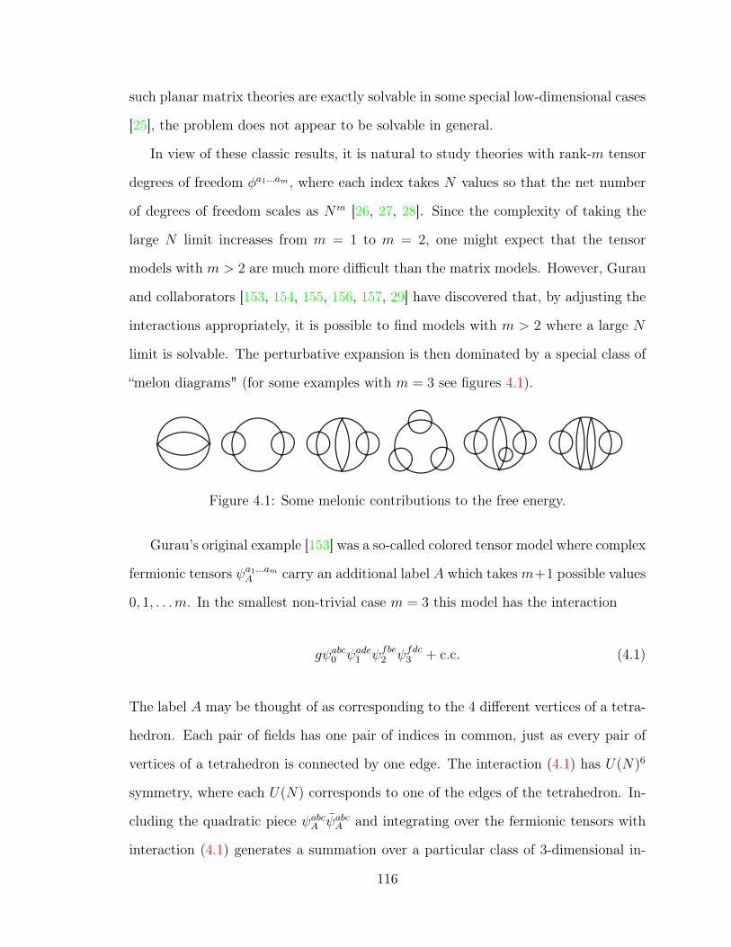
such planar matrix theories are exactly solvable in some special low-dimensional cases

[25], the problem does not appear to be solvable in general.

In view of these classic results, it is natural to study theories with rank-m tensor

degrees of freedom φa1...am , where each index takes N values so that the net number

of degrees of freedom scales as Nm [26, 27, 28]. Since the complexity of taking the

large N limit increases from m = 1 to m = 2, one might expect that the tensor

models with m > 2 are much more difficult than the matrix models. However, Gurau

and collaborators [153, 154, 155, 156, 157, 29] have discovered that, by adjusting the

interactions appropriately, it is possible to find models with m > 2 where a large N

limit is solvable. The perturbative expansion is then dominated by a special class of

“melon diagrams" (for some examples with m = 3 see figures 4.1).

Figure 4.1: Some melonic contributions to the free energy.

Gurau’s original example [153] was a so-called colored tensor model where complex

fermionic tensors ψa1...amA carry an additional label A which takesm+1 possible values

0, 1, . . .m. In the smallest non-trivial case m = 3 this model has the interaction

gψabc0 ψade1 ψfbe2 ψfdc3 + c.c. (4.1)

The label A may be thought of as corresponding to the 4 different vertices of a tetra-

hedron. Each pair of fields has one pair of indices in common, just as every pair of

vertices of a tetrahedron is connected by one edge. The interaction (4.1) has U(N)6

symmetry, where each U(N) corresponds to one of the edges of the tetrahedron. In-

cluding the quadratic piece ψabcA ψabcA and integrating over the fermionic tensors with

interaction (4.1) generates a summation over a particular class of 3-dimensional in-

116

trinsic geometries made out of tetrahedra. Apart from this interpretation, this model

is of much interest because it exhibits a novel type of large N limit, where the cou-

pling constant is scaled so that g2N3 is held constant, and the theory has N3 degrees

of freedom.1 Thus, it is interesting to try generalizing Gurau’s construction2 from the

d = 0 tensor integral case to d-dimensional quantum theories. An important step in

this direction was recently made by Witten [163], who studied a quantum mechanical

model of colored anti-commuting tensors and observed that its large N limit is similar

to that in the Sachdev-Ye-Kitaev (SYK) model [164, 165, 166, 167].

The quantum mechanical model introduced by Witten uses, in the m = 3 case,

real fermionic tensors ψabcA and possesses O(N)6 symmetry. The action of this model

is

SGurau−Witten =

∫dt( i

2ψabcA ∂tψ

abcA + gψabc0 ψade1 ψfbe2 ψfdc3

), (4.2)

It was shown [163, 168] that, in the large N limit of this model only the “melonic"

Feynman graphs survive, just as in the SYK model. Very importantly, gauging the

O(N)6 symmetry gets rid of the non-singlet states. This removes a crucial conceptual

obstacle in the search for the gravity dual of this model, in the spirit of the AdS/CFT

correspondence for gauge theories [169, 170, 171].

In work subsequent to [153] it was shown that the “coloring" is not necessary for

obtaining a large N limit where the melon graphs dominate, and theories of just one

complex bosonic tensor were shown to have this property [29, 172, 173, 174]. More

recently, a model of a single real rank-3 tensor with O(N)3 symmetry was studied

by Carrozza and Tanasa and shown to possess a melonic large N limit [30]. We will1The N3 scaling of the degrees of freedom is also found for 6-dimensional CFTs on N coincident

M5-branes [158, 159]. An interpretation of this scaling in terms of M2-branes with three holesattached to three different M5-branes, thus giving rise to tri-fundamental matter, was proposed insection 5.2 of [160]. One may wonder if there is a precise connection between theories on M5-branesand tensor models.

2The random tensor models also have connections with the “holographic space-time" approachto quantum gravity [161, 162].

117

study such a theory of one real rank-m fermionic tensor with interaction ψm+1. For

m = 3 the interaction assumes explicit form

VO(N)3 =1

4gψa1b1c1ψa1b2c2ψa2b1c2ψa2b2c1 (4.3)

The three indices are distinguishable, and the theory has O(N)3 symmetry under

ψabc →Maa′

1 M bb′

2 M cc′

3 ψa′b′c′ , M1,M2,M3 ∈ O(N) . (4.4)

Thus, the real field ψabc transforms in the tri-fundamental representation of O(N)3.

Such an O(N)3 fermionic model does not work in d = 0 because the invariant

quadratic term vanishes, ψabcψabc = 0, but in d = 1 there is a non-trivial model

with the kinetic term i2ψabc∂tψ

abc. We will also consider analogous bosonic models

where the anti-commuting field in (4.3) is replaced by a commuting one, φabc. Then

in d = 0 we may add the quadratic term φabcφabc, while in d > 0 the standard kinetic

term 12∂µφ

abc∂µφabc. While the bosonic potential is generally not positive definite,

the model may still be studied in perturbation theory. One may hope that, as in

the matrix models, the restriction to leading large N limit can formally stabilize the

theory.

In section 4.2 we study the index structure of the expansion of the path integral

in g and demonstrate that the large N limit is dominated by the melon diagrams.

3 The argument, which applies to both the O(N)3 fermionic and bosonic models,

contains a new ingredient compared to other models. In O(N)3 models with complex

tensors, which were studied in [29], each index loop necessarily passed through an

even number of vertices, but in models with real tensors a loop can also pass through3We constructed the argument before the existence of [30] was pointed out to us, so it may

provide an independent perspective on the O(N)3 theories.

118

an odd number of vertices. However, the diagrams dominant in the large N limit do

not contain any index loops that pass through 3 vertices.

In section 4.3 we show that the O(N)3 fermionic theory with interaction (4.3) is

equivalent to the SYK model in the large N limit. We comment on the spectrum

of operators in the gauged tensor models, pointing out that it appears to be vastly

bigger than the “single Regge trajectory" which has been studied in the SYK model

so far [175, 176, 177, 178]. In section 4.3.1 we write down a U(N)2×O(N) symmetric

quantum mechanical model with a complex fermionic 3-tensor. We study the large N

limit of this model and derive the scaling dimensions of two-particle operators. We

argue that this model is related in the large N limit to the generalization of SYK

model which contains complex fermions [179, 180].

It is of obvious interest to extend the SYK and tensor models to dimensions higher

than d = 1. Such extensions were considered in [31, 181, 182, 183, 184]. Some of our

work in this chapter will be following the observation that, in a theory of a rank-3

bosonic tensor field one may introduce quartic interactions with O(N)3 symmetry [31].

Although the action is typically unbounded from below, such a QFT is perturbatively

renormalizable in d = 4, so it may be studied using the 4− ε expansion [3].

In this chapter we explore the 4 − ε expansion and compare it with the large N

Schwinger-Dyson equations, finding perfect agreement. We present results on the

large N scaling dimensions of two-particle operators of arbitrary spin as a function

of d, found using the Schwinger-Dyson equations. A salient feature of the large N

spectrum of this theory in d < 4 is that the lowest scalar operator has a complex

dimension of the form d2

+ iα(d).4 We confirm this using the 4 − ε expansion in

section 4.4.3. In that calculation it is necessary to include the mixing of the basic4However, the scaling dimension of the lowest scalar operator is real for 4 < d < 4.155.

119

“tetrahedron" interaction term,

Ot(x) = φa1b1c1φa1b2c2φa2b1c2φa2b2c1 , (4.5)

with two additional O(N)3 invariant terms: the so-called pillow and double-sum

invariants (4.76). The coefficients of these additional terms turn out to be complex at

the “melonic" large N IR fixed point; as a result, the scaling dimension of the leading

operator φabcφabc is complex. A similar phenomenon for the O(N)2 symmetric theory

of a matrix φab is discussed in the Appendix A. In that case it is necessary to include

the O(N)2 invariant double-trace operator (φabφab)2 whose coefficient is complex at

the IR fixed point; as a result, the scaling dimension of operator φabφab is complex.

We also extend our results to rank q − 1 tensors with φq interactions. In each

dimension d it is found that the two-particle mode with complex scaling dimension

disappears for q greater than some critical value qcrit (for example, in d = 2, qcrit ≈ 64.3

[184]). We study the spectrum of bilinear operators in the large N bosonic theory

with q = 6 in 3 − ε dimensions and point out that it is free of the problem with

the complex dimension of φ2 for ε < 0.03. Thus, this theory is a candidate for a

stable large N CFT, albeit in a non-integer dimension. However, an obvious danger,

which we have not investigated, is that the coupling constants for some of the O(N)5

invariant sextic operators may be complex in d = 3− ε.

A more promising direction towards finding melonic CFTs in d ≥ 2 is to explore

the supersymmetric versions of tensor or SYK-like models [31, 184] and a successful

construction of such theory in d = 2 was achieved recently [184].

120

4.2 Melonic Dominance in the O(N)3 Symmetric

Theories

The arguments in this section, which are analogous to those in [30], apply to the

O(N)3 models, both in the fermionic and bosonic cases and for any d. We will ignore

the coordinate dependence and just focus on the index structure.

abc

abc

Figure 4.2: The resolved propagator 〈φabcφa′b′c′〉 = δaa′δbb′δcc′ .

The propagator of the φabc field has the index structure depicted in figure 4.2. The

three colored wires (also called “strands" in the earlier literature) represent propaga-

tion of the three indices of the φabc field. The vertex has the index structure depicted

in the figure 4.3. There are three equivalent ways to draw the vertex; for concreteness

we will use the first way. "Forgetting" the middle lines we obtain the standard matrix

model vertex as in figure 4.4.

Figure 4.3: Three equivalent ways to represent the resolved vertex.

Figure 4.4: The standard matrix model vertex obtained after “forgetting” the middlelines.

Let us consider the vacuum Feynman diagrams. Examples of melonic and non-

melonic diagrams with their resolved representations and fat (double-line) subgraphs

are depicted in figures 4.5 and 4.6.121

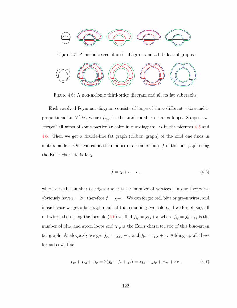
Figure 4.5: A melonic second-order diagram and all its fat subgraphs.

Figure 4.6: A non-melonic third-order diagram and all its fat subgraphs.

Each resolved Feynman diagram consists of loops of three different colors and is

proportional to N ftotal , where ftotal is the total number of index loops. Suppose we

“forget” all wires of some particular color in our diagram, as in the pictures 4.5 and

4.6. Then we get a double-line fat graph (ribbon graph) of the kind one finds in

matrix models. One can count the number of all index loops f in this fat graph using

the Euler characteristic χ

f = χ+ e− v , (4.6)

where e is the number of edges and v is the number of vertices. In our theory we

obviously have e = 2v, therefore f = χ+v. We can forget red, blue or green wires, and

in each case we get a fat graph made of the remaining two colors. If we forget, say, all

red wires, then using the formula (4.6) we find fbg = χbg+v, where fbg = fb+fg is the

number of blue and green loops and χbg is the Euler characteristic of this blue-green

fat graph. Analogously we get frg = χrg + v and fbr = χbr + v. Adding up all these

formulas we find

fbg + frg + fbr = 2(fb + fg + fr) = χbg + χbr + χrg + 3v . (4.7)

122

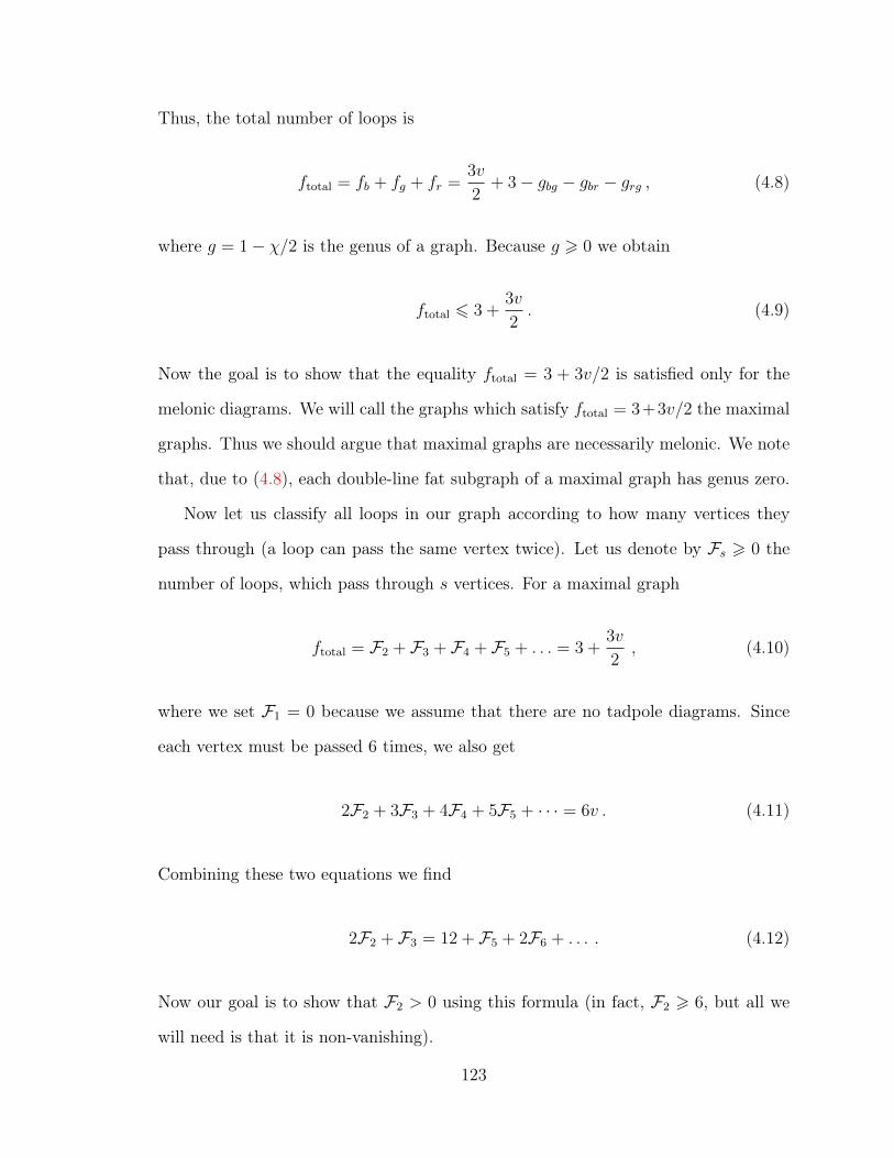
Thus, the total number of loops is

ftotal = fb + fg + fr =3v

2+ 3− gbg − gbr − grg , (4.8)

where g = 1− χ/2 is the genus of a graph. Because g > 0 we obtain

ftotal 6 3 +3v

2. (4.9)

Now the goal is to show that the equality ftotal = 3 + 3v/2 is satisfied only for the

melonic diagrams. We will call the graphs which satisfy ftotal = 3+3v/2 the maximal

graphs. Thus we should argue that maximal graphs are necessarily melonic. We note

that, due to (4.8), each double-line fat subgraph of a maximal graph has genus zero.

Now let us classify all loops in our graph according to how many vertices they

pass through (a loop can pass the same vertex twice). Let us denote by Fs > 0 the

number of loops, which pass through s vertices. For a maximal graph

ftotal = F2 + F3 + F4 + F5 + . . . = 3 +3v

2, (4.10)

where we set F1 = 0 because we assume that there are no tadpole diagrams. Since

each vertex must be passed 6 times, we also get

2F2 + 3F3 + 4F4 + 5F5 + · · · = 6v . (4.11)

Combining these two equations we find

2F2 + F3 = 12 + F5 + 2F6 + . . . . (4.12)

Now our goal is to show that F2 > 0 using this formula (in fact, F2 > 6, but all we

will need is that it is non-vanishing).

123

Let us first argue that a maximal graph must have F3 = 0. To have F3 > 0 we

need a closed index loop passing through 3 vertices. Without a loss of generality we

can assume that this loop is formed by the middle lines in each vertex (blue lines). The

only possibility with a closed loop of an internal (blue) index, which passes through

three vertices, is shown in fig. 4.7 a). After "forgetting" the color of this loop we get

a fat graph in fig. 4.7 b), which is non-planar due a twisted propagator. So, a graph

with F3 > 0 cannot be maximal. Thus, setting F3 = 0 in (4.12), we deduce that a

maximal graph should have F2 > 0.

Figure 4.7: a) Local part of a graph with a middle index loop passing through 3vertices. b) The same figure where the middle index has been “forgotten."

Finally, we need to show that the graphs with F2 > 0 are melonic. To do this

we will follow Proposition 3 in [157]. Without a loss of generality we assume that

the loop passing through 2 vertices is formed by the middle lines in each vertex (blue

lines). The only such possibility is shown in fig. 4.8 a). After "forgetting" the color

of this loop we get a fat graph in fig. 4.8 b).

Now we uncolor the lines in our fat graph and cut and sew two edges as in figure

4.9. We cut two edges but did not change the number of loops; therefore, the Euler

v1 v2 v1 v2

Figure 4.8: a) Local part of a graph with a middle index loop passing through twovertices v1 and v2. b) The same figure where the middle index has been “forgotten."

124

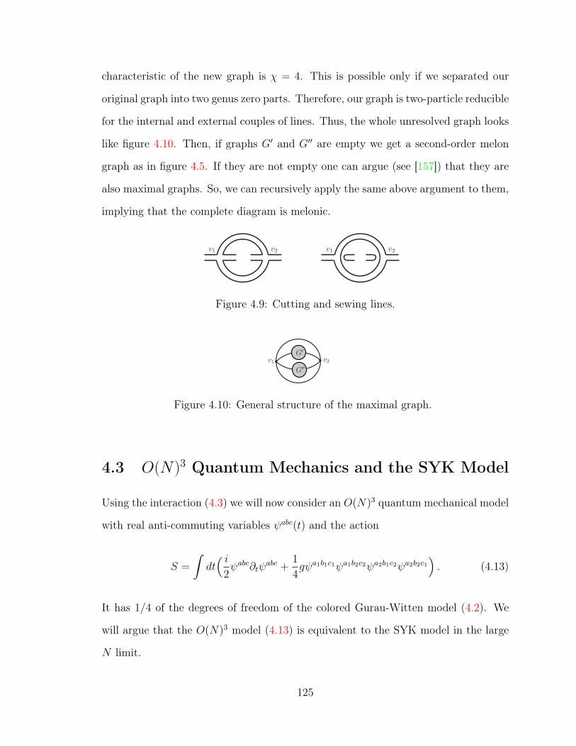
characteristic of the new graph is χ = 4. This is possible only if we separated our

original graph into two genus zero parts. Therefore, our graph is two-particle reducible

for the internal and external couples of lines. Thus, the whole unresolved graph looks

like figure 4.10. Then, if graphs G′ and G′′ are empty we get a second-order melon

graph as in figure 4.5. If they are not empty one can argue (see [157]) that they are

also maximal graphs. So, we can recursively apply the same above argument to them,

implying that the complete diagram is melonic.

v1 v2 v1 v2

Figure 4.9: Cutting and sewing lines.

G′

G′′v1 v2

Figure 4.10: General structure of the maximal graph.

4.3 O(N)3 Quantum Mechanics and the SYK Model

Using the interaction (4.3) we will now consider an O(N)3 quantum mechanical model

with real anti-commuting variables ψabc(t) and the action

S =

∫dt( i

2ψabc∂tψ

abc +1

4gψa1b1c1ψa1b2c2ψa2b1c2ψa2b2c1

). (4.13)

It has 1/4 of the degrees of freedom of the colored Gurau-Witten model (4.2). We

will argue that the O(N)3 model (4.13) is equivalent to the SYK model in the large

N limit.

125

We recall that ψabc are the N3 anticommuting fields and the indices, each of which

runs from 1 to N , are treated as distinguishable. The Fermi statistics implies

ψa1b1c1ψa1b2c2ψa2b1c2ψa2b2c1 = −ψa1b2c2ψa1b1c1ψa2b1c2ψa2b2c1 . (4.14)

After relabeling b1 ↔ c2 and b2 ↔ c1 we get the relation

ψa1b1c1ψa1b2c2ψa2b1c2ψa2b2c1 = −ψa1c1b1ψa1c2b2ψa2c2b1ψa2c1b2 . (4.15)

This demonstrates the vanishing of the interaction term in theO(N) symmetric theory

with a fully symmetric or fully anti-symmetric fermionic tensor. Fortunately, in the

theory with general 3-index fermionic tensors the interaction is non-trivial.

Let us return, therefore, to the theory (4.13) with O(N)3 symmetry, where the

three indices are distinguishable. The symmetry may be gauged by the replacement

∂tψabc → (Dtψ)abc = ∂tψ

abc + Aaa′

1 ψa′bc + Abb

′

2 ψab′c + Acc

′

3 ψabc′, (4.16)

where Ai is the gauge field corresponding to the i-th O(N) group. In d = 1 the gauge

fields are non-dynamical, and their only effect is to restrict the operators to be gauge

singlets. There is a sequence of such operators of the form

On2 = ψabc(Dn

t ψ)abc , (4.17)

where n is odd. This set of operators is analogous to the “single Regge trajectory"

[175, 176, 178] found in the Sachdev-Ye-Kitaev (SYK) model [164, 165, 166, 167].

We should note, however, that theory (4.13) contains an abundance of additional

“single-trace" O(N)3 symmetric operators. A large class of them contains an even

number of ψ fields without derivatives and with all indices contracted. One of such

126

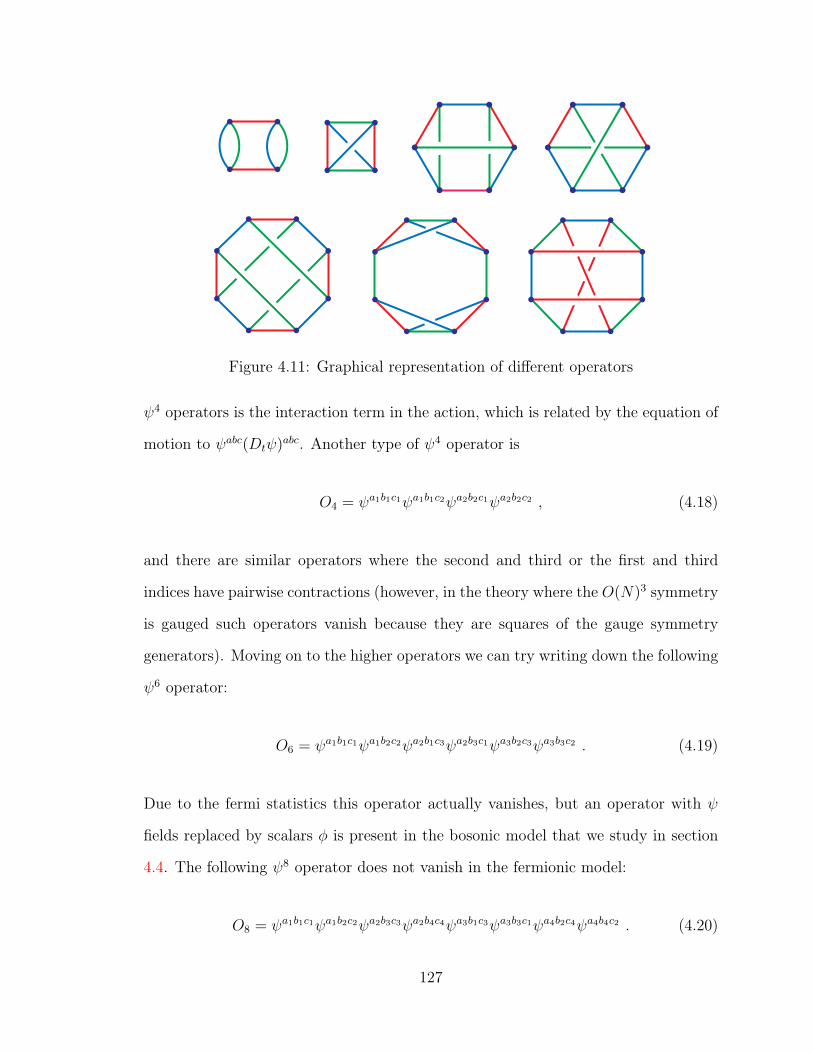
Figure 4.11: Graphical representation of different operators

ψ4 operators is the interaction term in the action, which is related by the equation of

motion to ψabc(Dtψ)abc. Another type of ψ4 operator is

O4 = ψa1b1c1ψa1b1c2ψa2b2c1ψa2b2c2 , (4.18)

and there are similar operators where the second and third or the first and third

indices have pairwise contractions (however, in the theory where the O(N)3 symmetry

is gauged such operators vanish because they are squares of the gauge symmetry

generators). Moving on to the higher operators we can try writing down the following

ψ6 operator:

O6 = ψa1b1c1ψa1b2c2ψa2b1c3ψa2b3c1ψa3b2c3ψa3b3c2 . (4.19)

Due to the fermi statistics this operator actually vanishes, but an operator with ψ

fields replaced by scalars φ is present in the bosonic model that we study in section

4.4. The following ψ8 operator does not vanish in the fermionic model:

O8 = ψa1b1c1ψa1b2c2ψa2b3c3ψa2b4c4ψa3b1c3ψa3b3c1ψa4b2c4ψa4b4c2 . (4.20)

127

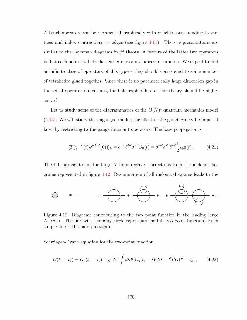
All such operators can be represented graphically with ψ-fields corresponding to ver-

tices and index contractions to edges (see figure 4.11). These representations are

similar to the Feynman diagrams in φ3 theory. A feature of the latter two operators

is that each pair of ψ-fields has either one or no indices in common. We expect to find

an infinite class of operators of this type – they should correspond to some number

of tetrahedra glued together. Since there is no parametrically large dimension gap in

the set of operator dimensions, the holographic dual of this theory should be highly

curved.

Let us study some of the diagrammatics of the O(N)3 quantum mechanics model

(4.13). We will study the ungauged model; the effect of the gauging may be imposed

later by restricting to the gauge invariant operators. The bare propagator is

〈T (ψabc(t)ψa′b′c′(0))〉0 = δaa

′δbb′δcc′G0(t) = δaa

′δbb′δcc′ 1

2sgn(t) . (4.21)

The full propagator in the large N limit receives corrections from the melonic dia-

grams represented in figure 4.12. Resummation of all melonic diagrams leads to the

. . . . . .

Figure 4.12: Diagrams contributing to the two point function in the leading largeN order. The line with the gray circle represents the full two point function. Eachsimple line is the bare propagator.

Schwinger-Dyson equation for the two-point function

G(t1 − t2) = G0(t1 − t2) + g2N3

∫dtdt′G0(t1 − t)G(t− t′)3G(t′ − t2) , (4.22)

128

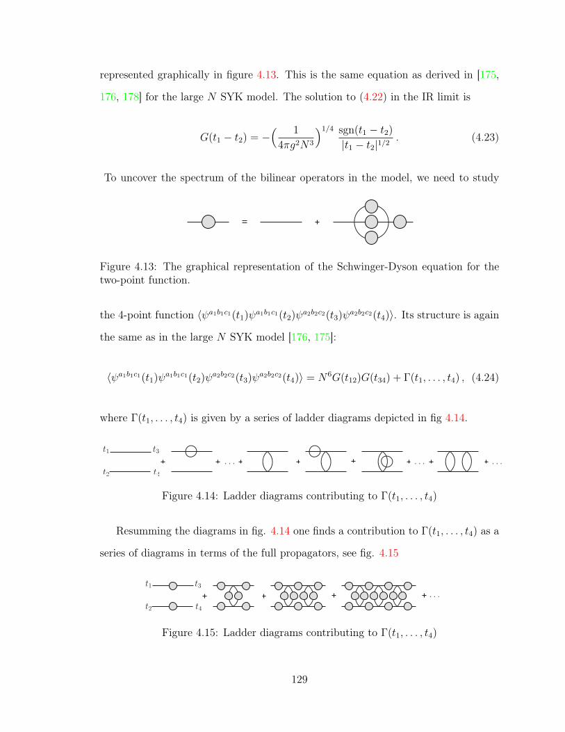
represented graphically in figure 4.13. This is the same equation as derived in [175,

176, 178] for the large N SYK model. The solution to (4.22) in the IR limit is

G(t1 − t2) = −( 1

4πg2N3

)1/4 sgn(t1 − t2)

|t1 − t2|1/2. (4.23)

To uncover the spectrum of the bilinear operators in the model, we need to study

Figure 4.13: The graphical representation of the Schwinger-Dyson equation for thetwo-point function.

the 4-point function 〈ψa1b1c1(t1)ψa1b1c1(t2)ψa2b2c2(t3)ψa2b2c2(t4)〉. Its structure is again

the same as in the large N SYK model [176, 175]:

〈ψa1b1c1(t1)ψa1b1c1(t2)ψa2b2c2(t3)ψa2b2c2(t4)〉 = N6G(t12)G(t34) + Γ(t1, . . . , t4) , (4.24)

where Γ(t1, . . . , t4) is given by a series of ladder diagrams depicted in fig 4.14.

t1 t3

t2 t4

. . . . . . . . .

Figure 4.14: Ladder diagrams contributing to Γ(t1, . . . , t4)

Resumming the diagrams in fig. 4.14 one finds a contribution to Γ(t1, . . . , t4) as a

series of diagrams in terms of the full propagators, see fig. 4.15

t1 t3

t2 t4

. . .

Figure 4.15: Ladder diagrams contributing to Γ(t1, . . . , t4)

129

If we denote by Γn the ladder with n rungs, so Γ =∑

n Γn, we have

Γ0(t1, . . . , t4) = N3(−G(t13)G(t24) +G(t14)G(t23)) . (4.25)

For the next coefficient one gets

Γ1(t1, . . . , t4) = 3g2N6

∫dtdt′

(G(t1 − t)G(t2 − t′)G(t− t′)2G(t− t3)G(t− t4)− (t3 ↔ t4)

),

(4.26)

and one can check further that

Γ2(t1, . . . , t4) = −3g2N3

∫dtdt′

(G(t1 − t)G(t2 − t′)G(t− t′)2Γ1(t, t′, t3, t4)− (t3 ↔ t4)

).

(4.27)

So, in general, one gets exactly the same recursion relation as in the SYK model

Γn+1(t1, . . . , t4) =

∫dtdt′K(t1, t2; t, t′)Γn(t, t′, t3, t4) , (4.28)

where the kernel is

K(t1, t2; t3, t4) = −3g2N3G(t13)G(t24)G(t34)2 . (4.29)

In order to find the spectrum of the two-particle operators On2 , following [176, 178]

one has to solve the integral eigenvalue equation

v(t0, t1, t2) = g(h)

∫dt3dt4K(t1, t2; t3, t4)v(t0, t3, t4) , (4.30)

130

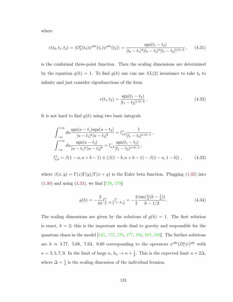
where

v(t0, t1, t2) = 〈On2 (t0)ψabc(t1)ψabc(t2)〉 =

sgn(t1 − t2)

|t0 − t1|h|t0 − t2|h|t1 − t2|1/2−h, (4.31)

is the conformal three-point function. Then the scaling dimensions are determined

by the equation g(h) = 1. To find g(h) one can use SL(2) invariance to take t0 to

infinity and just consider eigenfunctions of the form

v(t1, t2) =sgn(t1 − t2)

|t1 − t2|1/2−h. (4.32)

It is not hard to find g(h) using two basic integrals

∫ +∞

−∞du

sgn(u− t1)sgn(u− t2)

|u− t1|a|u− t2|b= l+a,b

1

|t1 − t2|a+b−1,∫ +∞

−∞du

sgn(u− t2)

|u− t1|a|u− t2|b= l−a,b

sgn(t1 − t2)

|t1 − t2|a+b−1,

l±a,b = β(1− a, a+ b− 1)± (β(1− b, a+ b− 1)− β(1− a, 1− b)) , (4.33)

where β(x, y) = Γ(x)Γ(y)/Γ(x + y) is the Euler beta function. Plugging (4.32) into

(4.30) and using (4.33), we find [176, 178]

g(h) = − 3

4πl+3

2−h, 1

2

l−1−h, 1

2

= −3

2

tan(π2(h− 1

2))

h− 1/2. (4.34)

The scaling dimensions are given by the solutions of g(h) = 1. The first solution

is exact, h = 2; this is the important mode dual to gravity and responsible for the

quantum chaos in the model [185, 175, 176, 177, 186, 187, 188]. The further solutions

are h ≈ 3.77, 5.68, 7.63, 9.60 corresponding to the operators ψabc(Dnt ψ)abc with

n = 3, 5, 7, 9. In the limit of large n, hn → n+ 12. This is the expected limit n+ 2∆,

where ∆ = 14is the scaling dimension of the individual fermion.

131

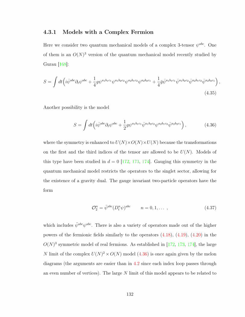
4.3.1 Models with a Complex Fermion

Here we consider two quantum mechanical models of a complex 3-tensor ψabc. One

of them is an O(N)3 version of the quantum mechanical model recently studied by

Gurau [168]:

S =

∫dt(iψabc∂tψ

abc +1

4gψa1b1c1ψa1b2c2ψa2b1c2ψa2b2c1 +

1

4gψa1b1c1ψa1b2c2ψa2b1c2ψa2b2c1

),

(4.35)

Another possibility is the model

S =

∫dt(iψabc∂tψ

abc +1

2gψa1b1c1ψa1b2c2ψa2b1c2ψa2b2c1

), (4.36)

where the symmetry is enhanced to U(N)×O(N)×U(N) because the transformations

on the first and the third indices of the tensor are allowed to be U(N). Models of

this type have been studied in d = 0 [172, 173, 174]. Gauging this symmetry in the

quantum mechanical model restricts the operators to the singlet sector, allowing for

the existence of a gravity dual. The gauge invariant two-particle operators have the

form

On2 = ψabc(Dnt ψ)abc n = 0, 1, . . . , (4.37)

which includes ψabcψabc. There is also a variety of operators made out of the higher

powers of the fermionic fields similarly to the operators (4.18), (4.19), (4.20) in the

O(N)3 symmetric model of real fermions. As established in [172, 173, 174], the large

N limit of the complex U(N)2×O(N) model (4.36) is once again given by the melon

diagrams (the arguments are easier than in 4.2 since each index loop passes through

an even number of vertices). The large N limit of this model appears to be related to

132

the variant of SYK model where the real fermions are replaced by the complex ones

[179, 180].

Let us briefly discuss summing over melonic graphs in the model (4.36) at large

N . The two-point function has the structure

〈T (ψabc(t)ψa′b′c′(0))〉 = δaa

′δbb′δcc′G(t), (4.38)

and G(t) = −G(−t). We find the same Schwinger-Dyson equation as (4.22); its

solution is again (4.23) indicating that the fermion scaling dimension is ∆ = 1/4. Now

we need to study the 4-point function 〈ψa1b1c1(t1)ψa1b1c1(t2)ψa2b2c2(t3)ψa2b2c2(t4)〉. It

leads to the same integral eigenvalue equation as (4.30), but with kernel

K(t1, t2; t3, t4) = −g2N3(2G(t13)G(t24)G(t34)2 −G(t14)G(t23)G(t34)2

). (4.39)

Now it is possible to have not only the antisymmetric eigenfunctions as in (4.32), but

also the symmetric ones

v(t1, t2) =1

|t1 − t2|1/2−h. (4.40)

This can be justified by noticing that the three point function now is 〈On2 (t0)ψabc(t1)ψabc(t2)〉.

We see that for odd n it is antisymmetric under t1 ↔ t2, while for even n it is sym-

metric.

Substituting ansatz (4.40) into the integral equation, and using the integrals

(4.33), we find

gsym(h) = − 1

4πl−3

2−h, 1

2

l+1−h, 1

2

= −1

2

tan(π2(h+ 1

2))

h− 1/2. (4.41)

133

The scaling dimensions of the operators On2 with even n are given by the solutions

of gsym(h) = 1. The first eigenvalue is h = 1, corresponding to the conserved U(1)

charge ψabcψabc. The additional values are h ≈ 2.65, 4.58, 6.55, 8.54 corresponding

to the operators with n = 2, 4, 6, 8 respectively. For large n the scaling dimensions

approach n + 12as expected. The numerical results are in good agreement with the

asymptotic formula [176]

hn = n+1

2+

1

πn+O(n−3) (4.42)

for n > 2. For On2 with odd n the spectrum is the same as for the two-particle

operators (4.17) in the model with O(N)3 symmetry.

4.4 O(N)3 bosonic tensors

In this section we consider the d-dimensional field theory of a real commuting tensor

field φabc(x) with distinguishable indices a, b, c = 1, . . . , N :

S =

∫ddx(1

2∂µφ

abc∂µφabc +1

4gφa1b1c1φa1b2c2φa2b1c2φa2b2c1

), (4.43)

This is the bosonic analogue of the O(N)3 fermionic theory with interaction (4.3); it

again has O(N)3 symmetry. A feature of this theory is that the interaction potential

is not bounded from below for N > 2. For N = 2 the potential may be written as

a sum of squares, but for N > 2 we have explicitly checked that there is a negative

direction. Nevertheless, we may consider formal perturbation theory in g.

The argument in section 4.2 that the melonic diagrams dominate in the large N

limit applies both to the fermionic and bosonic version of the theory in any dimension

d. We may therefore resum all such diagrams and derive the exact Schwinger-Dyson

134

equation similar to that in [154, 156, 155, 153, 189]. Let us explain this using a simple

example of the two-point function in the theory (4.43).

We have for the bare propagator

〈φabc(p)φa′b′c′(−p)〉0 = G0(p)δaa′δbb′δcc′=

1

p2δaa

′δbb′δcc′. (4.44)

In the large N limit one gets the same Schwinger-Dyson equation for the full two-point

function as in (4.22), which we can write in the momentum space as

G(p) = G0(p) + λ2G0(p)Σ(p)G(p) , (4.45)

where we introduced the coupling λ = gN3/2, which is held fixed in the large N limit

and

Σ(p) =

∫ddkddq

(2π)2dG(q)G(k)G(p+ q + k) . (4.46)

One can rewrite (4.45) as

G−1(p) = G−10 (p)− λ2Σ(p) . (4.47)

In the IR limit we can neglect the bare term G0(p) and get

G−1(p) = −λ2

∫ddkddq

(2π)2dG(q)G(k)G(p+ q + k) . (4.48)

Using the integral

∫ddk

(2π)d1

k2α(k + p)2β=

1

(4π)d/2Γ(d/2− α)Γ(d/2− β)Γ(α + β − d/2)

Γ(α)Γ(β)Γ(d− α− β)

1

(p2)α+β−d/2

(4.49)

135

it is not difficult to show that the solution to the equation (4.48) is

G(p) = λ−1/2((4π)ddΓ(3d

4)

4Γ(1− d4)

)1/4 1

(p2)d4

. (4.50)

Alternatively, one can work in the coordinate representation and use the Fourier

transform

∫ddx

eikx

(x2)α=πd/2Γ(d/2− α)

22α−dΓ(α)

1

(k2)d/2−α(4.51)

to find the solution of the equation G−1(x) = −λ2G3(x):

G(x) = λ−1/2( dΓ(3d

4)

4πdΓ(1− d4)

)1/4 1

(x2)d4

. (4.52)

If one works with the cutoff regularization, then the UV divergence, which arises in

the integrals can be absorbed into mass renormalization. Remarkably, the Schwinger-

Dyson equation (4.48) was originally studied in 1964, and its d = 3 solution (4.50)

was found [190].

4.4.1 Spectrum of two-particle operators

The O(N)3 invariant two-particle operators of spin zero have the form φabc(∂µ∂µ)nφabc,

where n = 0, 1, 2, . . .. At the quantum level these operators mix with each other,

although this mixing rapidly decreases as n increases, and the eigenvalues approach

2n+ d2.

Let us denote the conformal three-point function of a general spin zero operator

Oh with two scalar fields φabc by

v(x1, x2, x3) = 〈Oh(x1)φabc(x2)φabc(x3)〉 =COφφ

(x212x

213)

h2 (x2

23)12

(d/2−h), (4.53)

136

where h and ∆φ = d/4 are the scaling dimensions.

In the large N limit one can write the Schwinger-Dyson equation for the three-

point function [178]

v(x0, x1, x2) =

∫ddx3d

dx4K(x1, x2, x3, x4)v(x0, x3, x4) , (4.54)

where the kernel is given by the formula

K(x1, x2;x3, x4) = 3λ2G(x13)G(x24)G(x34)2 . (4.55)

This equation determines the possible values of scaling dimension h of the operator

Oh. Now using the general conformal integral [191]

∫ddx0

1

(x201)α1(x2

02)α2(x203)α3

=Ld(α1, α2)

(x212)

d2−α3(x2

13)d2−α2(x2

23)d2−α1

, (4.56)

where α1 + α2 + α3 = d and

Ld(α1, α2) = πd2

Γ(d2− α1)Γ(d

2− α2)Γ(d

2− α3)

Γ(α1)Γ(α2)Γ(α3)(4.57)

one can find that [31]

∫ddx3d

dx4K(x1, x2, x3, x4)v(x0, x3, x4) = g(h)v(x0, x1, x2) ,

g(h) = 3(Cφ)4Ld

(d4,h

2

)Ld

(d− h2

,d

4

)= − 3Γ

(3d4

)Γ(d4− h

2

)Γ(h2− d

4

)Γ(−d

4

)Γ(

3d4− h

2

)Γ(d4

+ h2

) . (4.58)

137

The dimensions of the spin zero operators in large N limit are determined by g(h) = 1.

In d = 4− ε this equation has solutions

h0 = 2± i√

6ε− 1

2ε+O(ε3/2), h1 = 4 + ε− 15ε2

4+O(ε3),

hn = 2(n+ 1)− ε

2+

3ε2

2n2(n2 − 1)+O(ε3), for n > 1 . (4.59)

We note that the first scaling dimension, h0, is complex, which means that the crit-

ical point is unstable. From the AdS5−ε side the relation between mass and scaling

dimension

h =d

2±√d2

4+m2 (4.60)

gives

m2 = −4− 4ε+ 11ε2 +O(ε3) , (4.61)

which is slightly below the Breitenlohner-Freedman [192] bound m2 > −d2/4.

More generally, for d < 4, the first solution of g(h) = 1 has the form

h0 =d

2± iα(d) , (4.62)

where α(d) is real. This is in agreement with (4.60) for m2 < −d2/4. On the other

hand, for 4 < d < 4.155, h0 is real and the large N theory is free of this instability,

at least formally.

138

4.4.2 Spectrum of higher-spin operators

Consider a higher-spin operator Js(x) = zµ1 . . . zµsJµ1...µs , where we introduced an

auxiliary null vector zµ, satisfying

z2 = zµzνδµν = 0 . (4.63)

The three-point function 〈Jsφabcφabc〉 is completely fixed by conformal invariance

〈Js(x1)φabc(x2)φabc(x3)〉 = Cs00

(z·x12

x212− z·x13

x213

)s(x2

12)τs2 (x2

23)∆φ− τs2 (x231)

τs2

, (4.64)

where ∆φ = d/4 and τs = ∆Js−s and ∆Js = 2∆φ+s+γs. If we set the Js momentum

to zero or equivalently, integrate over the position of Js we get

vs(x2, x3) =

∫ddx1〈Js(x1)φabc(x2)φabc(x3)〉 =

(z · x23)s

(x223)

τs2

+s− d2

+∆φ

. (4.65)

In the large N limit one can again write the Schwinger-Dyson equation for the three-

point function

vs(x1, x2) =

∫ddx3d

dx4K(x1, x2, x3, x4)vs(x3, x4) . (4.66)

To perform the integral in the r.h.s of (4.66) we use the well-known integral

∫ddx

(z · x)s

x2α(x− y)2β= Ld,s(α, β)

(z · y)s

(y2)α+β−d/2 ,

Ld,s(α, β) = πd/2Γ(d2− α + s

)Γ(d2− β

)Γ(α + β − d

2

)Γ(α)Γ(β)Γ(d+ s− α− β)

. (4.67)

139

Using (4.67) we find

∫ddx3d

dx4K(x1, x2, x3, x4)vs(x3, x4) = g(τs, s)vs(x1, x2) ,

g(τs, s) = 3(Cφ)4Ld,s

(d4

+ s+τs2,d

4

)Ld,s

(s+

τs2,d

4

)= − 3Γ

(3d4

)Γ(d−2τs

4)Γ(4s+2τs−d

4)

Γ(−d

4

)Γ(3d−2τs

4)Γ(d+4s+2τs

4)

(4.68)

and to find the spectrum we have to solve the equation g(τs, s) = 1. Note that for any

d, there is a solution with s = 2 and τs = d − 2. This corresponds to the conserved

stress tensor, consistently with the conformal invariance.

For general fixed spin s, the dimensions should approach, at large n

∆Js = 2∆φ + s+ 2n, n = 0, 1, 2, . . . , (4.69)

where n is interpreted as the number of contracted derivatives. Alternatively, one can

also study the behavior for large spin s, and fixed n (say n = 0), where the dimensions

should approach ∆Js ≈ 2∆φ+s+c/sτmin , where τmin is the lowest twist (excluding the

identity) appearing in the OPE expansion of the φ 4-point function [193, 194, 195].

For n = 0 we have in d = 4− ε

τs = d− 2 +(s− 2)(s+ 3)

2s(s+ 1)ε+ . . . . (4.70)

Note that the correction to d − 2 vanishes for s = 2, as it should since the stress

tensor is conserved. The fact that this correction for s 6= 2 is ∼ ε also makes sense,

because for nearly conserved currents the anomalous dimension starts at ∼ g2 on

general grounds (like γφ). The spin dependence in the above result is the expected

one for an almost conserved current near d = 4, see e.g. [196, 197].

140

In d = 2 the equation determining the dimensions becomes elementary and reads

3

(1− τs)(2s+ τs − 1)= 1 (4.71)

with solutions

τs = 1− s±√s2 − 3 . (4.72)

Surprisingly, this gives only one solution with h > d/2 for each spin, rather than the

infinite number of solutions which are present in d > 2 (already in d = 2 + ε there are

towers of real solutions). For s = 0 in d = 2 the solution (4.72) is complex

h ≈ 1 + 1.5235i . (4.73)

In d = 2 + ε there is also a tower of real solutions:5

τs = 2n+d

2+

3

3 + 4n(n+ s)ε+O(ε2) . (4.74)

In d = 1 the primary two-particle operators have the form φabc∂2nt φ

abc, where n =

0, 1, 2, . . .. The graphical solution of the eigenvalue equation is shown in figure 4.16.

The equation has a symmetry under h→ 1−h. The first real solution greater than 1/2

is the exact solution h = 2. It correspond to the n = 1 operator, which through the

use of equations of motion is proportional to the potential φa1b1c1φa1b2c2φa2b1c2φa2b2c1 .

The first eigenvalue is complex, h0 = 12

+ 1.525i. Since it is of the form 12

+ is, it is a

normalizable mode which needs to be integrated over, similarly to the h = 2 mode.5In the ε→ 0 limit it appears to give additional states in d = 2 which are missed by the degenerate

d = 2 equation (4.71).

141

y=g(h)

y=1

h=2 h=4.26 h=6.34 h=8.38

2 4 6 8 10h

-2

-1

1

2

3

g(h)

Figure 4.16: The graphical solution of the eigenvalue equation g(h) = 1 in d = 1.

4.4.3 Complex Large N Fixed Point in d = 4− ε

In this section we study the renormalizable theory in 4− ε dimensions with a 3-tensor

degree of freedom and O(N)3 symmetric quartic interactions:

S =

∫ddx(1

2∂µφ

abc∂µφabc +1

4

(g1Ot(x) + g2Op(x) + g3Ods(x)

)), (4.75)

where g1, g2, g3 are the bare couplings which correspond to the three possible invariant

quartic interaction terms. The perturbative renormalizability of the theory requires

that, in addition to the “tetrahedron" interaction term (4.5), we introduce the “pillow"

and “double-sum" terms

Op(x) =1

3

(φa1b1c1φa1b1c2φa2b2c2φa2b2c1 + φa1b1c1φa2b1c1φa2b2c2φa1b2c2

+ φa1b1c1φa1b2c1φa2b1c2φa2b2c2),

Ods(x) = φa1b1c1φa1b1c1φa2b2c2φa2b2c2 . (4.76)

To find the beta functions we use a well-known result [59] for a general φ4-model with

the interaction term V = 14gijklφ

iφjφkφl. In our case we can write interaction as

V =1

4gκ1κ2κ3κ4φ

κ1φκ2φκ4φκ4 , (4.77)

142

where κi = (aibici) is a set of three indices and gκ1κ2κ3κ4 is a sum of three structures

gκ1κ2κ3κ4 = g1Ttκ1κ2κ3κ4

+ g2Tpκ1κ2κ3κ4

+ g3Tdsκ1κ2κ3κ4

. (4.78)

Each structure is a sum of a product of Kronecker-delta terms, which after contraction

with φκ1φκ2φκ4φκ4 reproduce (4.5) and (4.76). For example

T tκ1κ2κ3κ4=

1

4!

(δa1a2δb1b3δc1c4δb2b4δc2c3δa3a4 + sym(κ1, . . . , κ4)

), (4.79)

where the last term means that we have to add all terms corresponding to permuta-

tions of κ1, . . . , κ4. Using the explicit formulas in [59], we find the beta functions up

to two loops

βt =− εg1 +4

3(4π)2

(3g1g2(N + 1) + 18g1g3 + 2g2

2

)+

2

9(4π)4

(9(N3 − 15N − 10)g3

1 − 36g21

((N2 + 4N + 13)g2 + 15Ng3

)− 3g1

((N3 + 15N2 + 93N + 101)g2

2 + 12(5N2 + 17N + 17)g2g3 + 6(5N3 + 82)g23

)− 4g2

2

((2N2 + 13N + 24)g2 + 72g3

)), (4.80)

βp =− εg2 +2

3(4π)2

(9g2

1(N + 2) + 12g2g1(N + 2) + g22(N2 + 5N + 12) + 36g2g3

)− 2

9(4π)4

(108(N2 +N + 4)g3

1 + 9g21

((N3 + 12N2 + 99N + 98)g2 + 72(N + 2)g3

)+ 36g1g2

((4N2 + 18N + 29)g2 + 3(13N + 16)g3

)+ g2

((5N3 + 45N2 + 243N + 343)g2

2

+ 36(7N2 + 15N + 29)g2g3 + 18(5N3 + 82)g23

)), (4.81)

143

and

βds =− εg3 +2

3(4π)2

(3g2

3

(N3 + 8

)+ 6g3g2

(N2 +N + 1

)+ g2

2(2N + 3) + 18g1g3N + 6g1g2

)− 2

9(4π)4

(54Ng3

1 + 9g21

(4(N2 +N + 4)g2 + 5(N3 + 3N + 2)g3

)+ 36g1

(4(N + 1)g2

2 + (5N2 + 5N + 17)g2g3 + 33Ng23

)+ 14(N2 + 3N + 5)g3

2

+ 3(5N3 + 15N2 + 93N + 97)g22g3 + 396(N2 +N + 1)g2g

23 + 54(3N3 + 14)g3

3

).

(4.82)

For the anomalous dimension we obtain

γφ =1

6(4π)4

(3g2

1(N3 + 3N + 2) + 6g23(N3 + 2) + 12g1

(g2(N2 +N + 1) + 3g3N

)+ 12g2g3(N2 +N + 1) + g2

2(N3 + 3N2 + 9N + 5)). (4.83)

Now, using the large N scaling

g1 =(4π)2g1

N3/2, g2 =

(4π)2g2

N2, g3 =

(4π)2g3

N3, (4.84)

where gi are held fixed, we find that the anomalous dimension

γφ =g2

1

2+O(1/N) (4.85)

and the beta functions

βt =− εg1 + 2g31 ,

βp =− εg2 +(

6g21 +

2

3g2

2

)− 2g2

1 g2 ,

βds =− εg3 +(4

3g2

2 + 4g2g3 + 2g23

)− 2g2

1(4g2 + 5g3) . (4.86)

144

We note that βt depends only on the tetrahedron coupling g1, while the beta functions

for pillow and double-sum also contain g1. This is a feature of the large N limit.

Similarly, in the large N limit of the quartic matrix theory, the double-trace coupling

does not affect the beta function of the single-trace coupling (see the Appendix).

The large N critical point with a non-vanishing tetrahedron coupling is

g∗1 = (ε/2)1/2, g∗2 = ±3i(ε/2)1/2, g∗3 = ∓i(3±√

3)(ε/2)1/2 . (4.87)

For the dimension of the O = φabcφabc operator at large N we find

∆O = d− 2 + 2(g∗2 + g∗3) = 2± i√

6ε+O(ε) . (4.88)

This exactly coincides with the large N solution (4.59), providing a nice perturbative

check of the fact that the scaling dimension is complex. We note that the imaginary

part originates from the complex pillow and double-sum couplings.

Now if we look for the dimension of the tetrahedron operator, then using the

derivative of the beta function, we find

∆tetra = d+ β′t(g∗1) = 4 + ε+O(ε2) , (4.89)

which coincides with the scaling dimension h1 of operator φabc∇2φabc found in (4.59).

4.4.4 Generalization to Higher q

The construction of theories for a single rank 3 tensor field with the quartic interaction

(4.43) may be generalized to a single rank q − 1 tensor with the O(N)q−1 symmetric

interaction of order q. Since the indices of each O(N) group must be contracted

pairwise, q has to be even. The rank q − 1 tensor theories have a large N limit with

λ2 = g2N (q−1)(q−2)/2 held fixed, which is dominated by the melonic diagrams (this

145

follows from the method of “forgetting" all but two colors in the graphs made out

of q − 1 strands by analogy with the derivation [157, 30, 163, 31] for q = 4). For

example, for q = 6 the explicit form of the interaction of a real rank 5 tensor is [31]

Vint =g

6φa1b1c1d1e1φa1b2c2d2e2φa2b2c3d3e1φa2b3c2d1e3φa3b3c1d3e2φa3b1c3d2e3 . (4.90)

Since every pair of fields have one index in common, this interaction may be repre-

sented by a 5-simplex.

The two-point Schwinger-Dyson equation has the form

G−1(x) = −λ2G(x)q−1 . (4.91)

The general d solution to this equation is

G(x) =Cφλ2/q

1

(x2)dq

,

Cφ =

(−π−dΓ(d

q)Γ(d(q−1)

q)

Γ(d(2−q)2q

)Γ(d(q−2)2q

)

)1/q

. (4.92)

In analogy to Section (4.4.1) one can find a spectrum of spin zero operators by

solving Schwinger-Dyson equation for the three-point function

v(x0, x1, x2) =

∫ddx3d

dx4K(x1, x2, x3, x4)v(x0, x3, x4) , (4.93)

where the kernel is given by the formula

K(x1, x2;x3, x4) = (q − 1)λ2G(x13)G(x24)G(x34)q−2 . (4.94)

146

Using the integral (4.56) and expression (4.92) we find

gq(h) = (q − 1)(Cφ)qLd

(dq,h

2

)Ld

(d− h2

,d

q

)= −

(q − 1)Γ(d(q−2)2q

)Γ(d(q−1)q

)Γ(h2− d(q−2)

2q)Γ(d

q− h

2)

Γ(d(2−q)2q

)Γ(dq)Γ(h

2+ d(q−2)

2q)Γ(d(q−1)

q− h

2)

, (4.95)

where Cφ is given in (4.92).

By solving gq(h) = 1 we find the spectrum of dimensions of spin zero two-particle

operators. As we already noticed in (4.4.1), for q = 4 the lowest operator O = φ2 has

complex dimension, which signals an instability of the theory. However, for d greater

than the critical value dcr, there exists qcrit such that for q > qcrit the solutions of

gq(h) = 1 are real, and the two-particle operators do not cause instabilities. The dcr

is determined byΓ(−dcr/4)2Γ(dcr/2)Γ(dcr + 1)

Γ(−dcr/2)Γ(3dcr/4)2= −1 , (4.96)

and we find dcr ≈ 1.93427. Interestingly, qcrit diverges at dcr as qcrit ≈ 4.092d−dcr . The plot

for qcrit as a function of d is shown in Figure 4.17.

In d = 2, the critical value of q is still large: qcrit ≈ 64.3 [184], but it drops to

≈ 5.9 in d = 3. For d < dcr the lowest eigenvalue is complex for any q. In d = 1, in

the large q limit

h0 =1

2+ i

√7

2+O(1/q) . (4.97)

147

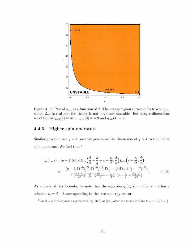
UNSTABLE

q=64.3

q=5.895q=4

2.0 2.5 3.0 3.5 4.0

10

20

30

40

50

60

70

d

q

Figure 4.17: Plot of qcrit as a function of d. The orange region corresponds to q > qcrit,where ∆φ2 is real and the theory is not obviously unstable. For integer dimensionswe obtained qcrit(2) ≈ 64.3, qcrit(3) ≈ 5.9 and qcrit(4) = 4.

4.4.5 Higher spin operators

Similarly to the case q = 4, we may generalize the discussion of q > 4 to the higher

spin operators. We find that 6

gq(τs, s) =(q − 1)(Cφ)qLd,s

(d2− d

q+ s+

τs2,d

q

)Ld,s

(s+

τs2,d

q

)=−

(q − 1)Γ(d(q−2)2q

)Γ(d(q−1)q

)Γ(dq− τs

2)Γ(s+ τs

2− d(q−2)

2q)

Γ(d(2−q)2q

)Γ(dq)Γ(d(q−1)

q− τs

2)Γ(s+ τs

2+ d(q−2)

2q)

. (4.98)

As a check of this formula, we note that the equation gq(τs, s) = 1 for s = 2 has a

solution τs = d− 2 corresponding to the stress-energy tensor.6For d = 2, this equation agrees with eq. (6.8) of [184] after the identifications h = s+ τ

2 , h = τ2 .

148

Similarly to the case q = 4, which degenerates for d = 2, we find a similar

degeneration of (4.98) for q = 8 and d = 4,

g(τs, s) =315

(τs − 5)(τs − 3)(τs − 1)(2s+ τs − 3)(2s+ τs − 1)(2s+ τs + 1), (4.99)

and the equation g = 1 may be solved in terms of the square and cubic roots. The

physically relevant solution for τ has the large s expansion

τs = 1 +315

64s3+

315

64s5+ . . . . (4.100)

More generally, we have checked numerically that, in the large s limit, τ → 2∆φ,

where ∆φ = d/q. For example, for q = 6 and d = 2, we find

τ4 = 0.456 , τ6 = 0.547 , τ1000 ≈ 0.666 . (4.101)

4.4.6 A Melonic φ6 Theory in 2.99 Dimensions

Using (4.95) for q = 6 we find that the spin zero spectrum is free of complex solutions

in a small region of dimension below 3. Working in d = 3− ε, we find that the scaling

dimensions are real for ε < 0.02819. Expansions of the first three solutions of the

equation g6(h) = 1 are

h− = 1 +29ε

3+

400ε2

9+

160

27

(237 + 2π2

)ε3 +O(ε4) ,

h+ = 2− 32ε

3− 400ε2

9− 160

27

(237 + 2π2

)ε3 +O(ε4) ,

h1 = 3 + 3ε− 220ε2

9+

40

81

(503 + 3π2

)ε3 +O(ε4) , (4.102)

149

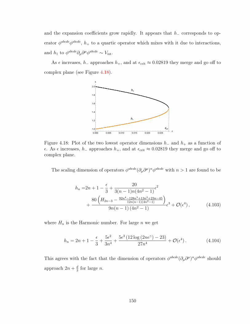
and the expansion coefficients grow rapidly. It appears that h− corresponds to op-

erator φabcdeφabcde, h+ to a quartic operator which mixes with it due to interactions,

and h1 to φabcde∂µ∂µφabcde ∼ Vint.

As ε increases, h− approaches h+, and at εcrit ≈ 0.02819 they merge and go off to

complex plane (see Figure 4.18).

h+

h-

ϵcr

0.000 0.005 0.010 0.015 0.020 0.025ϵ

1.0

1.2

1.4

1.6

1.8

2.0

h

Figure 4.18: Plot of the two lowest operator dimensions h− and h+ as a function ofε. As ε increases, h− approaches h+, and at εcrit ≈ 0.02819 they merge and go off tocomplex plane.

The scaling dimension of operators φabcde(∂µ∂µ)nφabcde with n > 1 are found to be

hn =2n+ 1− ε

3+

20

3(n− 1)n(4n2 − 1)ε2

+80(H2n−3 − 92n4−128n3+13n2+23n−45

12n(n−1)(4n2−1)

)9n(n− 1) (4n2 − 1)

ε3 +O(ε4) , (4.103)

where Hn is the Harmonic number. For large n we get

hn = 2n+ 1− ε

3+

5ε2

3n4+

5ε3 (12 log (2neγ)− 23)

27n4+O(ε4) . (4.104)

This agrees with the fact that the dimension of operators φabcde(∂µ∂µ)nφabcde should

approach 2n+ d3for large n.

150

For operators of s > 0, we may use (4.98) to obtain for n = 0

h(s) = d− 2 + s+8(s2 − 4)

3(4s2 − 1)ε

− 20

3 (4s2 − 1)

(ψ(s− 1

2)− ψ(

3

2)− 2(s− 2) (20s3 + 4s2 + 43s+ 5)

3 (4s2 − 1)2

)ε2 +O(ε3) .

(4.105)

The first term is the dimension of the operator in free field theory, while the additional

terms appear due to the φ6 interactions.

It would be interesting to reproduce the 3 − ε expansions found in this section

using perturbative calculations in the O(N)5 invariant renormalizable φ6 theory. This

is technically more complicated than the similar calculation we carried out in 4 − ε

dimensions, because there are several invariant φ6 terms. An obvious danger is that

the coupling constants for some of the sextic operators will be complex in d = 3− ε.

We hope to return to these issues in the future.

4.5 Appendix A. Matrix model in d = 4−ε dimension

In this appendix we consider renormalizable theory in 4− ε dimensions with a matrix

degree of freedom and O(N)2 symmetric quartic interactions:

S =

∫ddx(1

2∂µφ

ab∂µφab +1

4g1Ost(x) +

1

4g2Odt(x)

), (4.106)

where g1, g2 are the bare couplings which correspond to the two possible invariant

quartic interaction terms. The perturbative renormalizability of the theory requires

that, in addition to the single-trace term

Ost(x) = φabφcbφcdφad = TrφφTφφT , (4.107)

151

we introduce the double-trace term

Odt(x) = φabφabφcdφcd = TrφφTTrφφT . (4.108)

In analogy with the section 4.4.3 we find the beta functions using a well-known result

[59] for a general φ4-model with the interaction vertex V = 14gijklφ

iφjφkφl. The beta

functions up to two loops are

βst =− εg1 +g1(g1(N + 2) + 6g2)

4π2

− g1 (3g21(N(N + 6) + 17) + 4g1g2(22N + 29) + 2g2

2 (5N2 + 82))

128π4,

βdt =− εg2 +3g2

1 + 2g1g2(2N + 1) + g22 (N2 + 8)

8π2

− 6g31(2N + 3) + g2

1g2(5N(N + 2) + 87) + 44g1g22(2N + 1) + 6g3

2 (3N2 + 14)

128π4.

(4.109)

Now, using the large N scaling

g1 =(4π)2g1

N, g2 =

(4π)2g2

N2, (4.110)

where gi are held fixed, we find the beta functions

βst =− εg1 + 4g21 − 6g3

1 ,

βdt =− εg2 +(6g2

1 + 2g22 + 8g1g2

)− 2g2

1(12g1 + 5g2) . (4.111)

We note that βst depends only on the single-trace coupling g1, while the double-

trace beta function depends on both couplings. This is a familiar phenomenon for

beta functions in large N matrix theories [198]. Comparing with the beta functions

(4.80–4.82) of the large N 3-tensor theory, we observe that the tetrahedron coupling

in the tensor model is analogous to the single-trace coupling in the matrix model,

152

while the pillow and double-sum couplings in the tensor model are analogous to the

double-trace coupling in the matrix model.

The large N critical point with a non-vanishing single-trace coupling is

g∗1 =ε

4+

3ε2

32, g∗2 = −1

4

(1± i

√2)ε− 1

32

(1∓ 2i

√2)ε2 . (4.112)

For the dimension of the O = φabφab operator at large N we find

∆O = d− 2 + 4g∗1 + 2g∗2 = 2− 1

2

(1± i

√2)ε+O(ε2) . (4.113)

The imaginary part originates from the double-trace coupling. So, in spite of the

positivity of the interaction term Ost, this large N critical point is unstable due to an

operator dimension being complex. The form of the dimension, d2

+ iα, corresponds

to a field violating the Breitenlohner-Freedman bound in the dual AdS space.

153

Bibliography

[1] J. C. Le Guillou and J. Zinn-Justin, “Critical Exponents from Field Theory,”

Phys. Rev., vol. B21, pp. 3976–3998, 1980.

[2] L. D. Landau, “On the theory of phase transitions,” Zh. Eksp. Teor. Fiz., vol. 7,

pp. 19–32, 1937.

[3] K. G. Wilson and M. E. Fisher, “Critical exponents in 3.99 dimensions,”

Phys.Rev.Lett., vol. 28, pp. 240–243, 1972.

[4] S. El-Showk, M. F. Paulos, D. Poland, S. Rychkov, D. Simmons-Duffin, and

A. Vichi, “Solving the 3d Ising Model with the Conformal Bootstrap II. c-

Minimization and Precise Critical Exponents,” J. Stat. Phys., vol. 157, p. 869,

2014.

[5] R. Guida and J. Zinn-Justin, “Critical exponents of the N vector model,”

J.Phys., vol. A31, pp. 8103–8121, 1998.

[6] K. G. Wilson and J. B. Kogut, “The Renormalization group and the epsilon

expansion,” Phys. Rept., vol. 12, pp. 75–200, 1974.

[7] A. M. Polyakov, “Nonhamiltonian approach to conformal quantum field theory,”

Zh. Eksp. Teor. Fiz., vol. 66, pp. 23–42, 1974. [Sov. Phys. JETP39,9(1974)].

154

[8] S. Ferrara, A. F. Grillo, and R. Gatto, “Tensor representations of conformal

algebra and conformally covariant operator product expansion,” Annals Phys.,

vol. 76, pp. 161–188, 1973.

[9] S. Ferrara, R. Gatto, and A. F. Grillo, “Positivity Restrictions on Anomalous

Dimensions,” Phys. Rev., vol. D9, p. 3564, 1974.

[10] S. El-Showk, M. F. Paulos, D. Poland, S. Rychkov, D. Simmons-Duffin, and

A. Vichi, “Solving the 3D Ising Model with the Conformal Bootstrap,” Phys.

Rev., vol. D86, p. 025022, 2012.

[11] S. El-Showk, Y. Nakayama, and S. Rychkov, “What Maxwell Theory in D 6=

4 teaches us about scale and conformal invariance,” Nucl. Phys., vol. B848,

pp. 578–593, 2011.

[12] J. S. Schwinger, “Gauge Invariance and Mass. 2.,” Phys.Rev., vol. 128, pp. 2425–

2429, 1962.

[13] T. Appelquist and R. D. Pisarski, “High-Temperature Yang-Mills Theories and

Three-Dimensional Quantum Chromodynamics,” Phys. Rev., vol. D23, p. 2305,

1981.

[14] T. Appelquist, D. Nash, and L. C. R. Wijewardhana, “Critical Behavior in

(2+1)-Dimensional QED,” Phys. Rev. Lett., vol. 60, p. 2575, 1988.

[15] M. Moshe and J. Zinn-Justin, “Quantum field theory in the large N limit: A

Review,” Phys. Rept., vol. 385, pp. 69–228, 2003.

[16] M. Beneke and V. A. Smirnov, “Ultraviolet renormalons in Abelian gauge the-

ories,” Nucl. Phys., vol. B472, pp. 529–590, 1996.

[17] L. Di Pietro, Z. Komargodski, I. Shamir, and E. Stamou, “Quantum Electro-

dynamics in d=3 from the epsilon-expansion,” 2015.155

[18] J. B. Marston and I. Affleck, “Large-n limit of the Hubbard-Heisenberg model,”

Phys. Rev., vol. B39, pp. 11538–11558, 1989.

[19] M. Franz, Z. Tesanovic, and O. Vafek, “QED(3) theory of pairing pseudogap

in cuprates. 1. From D wave superconductor to antiferromagnet via ’algebraic’

Fermi liquid,” Phys. Rev., vol. B66, p. 054535, 2002.

[20] I. F. Herbut, “QED(3) theory of underdoped high temperature superconduc-

tors,” Phys. Rev., vol. B66, p. 094504, 2002.

[21] R. D. Pisarski, “Chiral Symmetry Breaking in Three-Dimensional Electrody-

namics,” Phys. Rev., vol. D29, p. 2423, 1984.

[22] T. W. Appelquist, M. J. Bowick, D. Karabali, and L. C. R. Wijewardhana,

“Spontaneous Chiral Symmetry Breaking in Three-Dimensional QED,” Phys.

Rev., vol. D33, p. 3704, 1986.

[23] C. Vafa and E. Witten, “Eigenvalue Inequalities for Fermions in Gauge Theo-

ries,” Commun. Math. Phys., vol. 95, p. 257, 1984.

[24] G. ’t Hooft, “A Planar Diagram Theory for Strong Interactions,” Nucl. Phys.,

vol. B72, p. 461, 1974.

[25] E. Brezin, C. Itzykson, G. Parisi, and J. B. Zuber, “Planar Diagrams,” Commun.

Math. Phys., vol. 59, p. 35, 1978.

[26] J. Ambjorn, B. Durhuus, and T. Jonsson, “Three-dimensional simplicial quan-

tum gravity and generalized matrix models,” Mod. Phys. Lett., vol. A6,

pp. 1133–1146, 1991.

[27] N. Sasakura, “Tensor model for gravity and orientability of manifold,” Mod.

Phys. Lett., vol. A6, pp. 2613–2624, 1991.

156

[28] M. Gross, “Tensor models and simplicial quantum gravity in > 2-D,” Nucl.

Phys. Proc. Suppl., vol. 25A, pp. 144–149, 1992.

[29] V. Bonzom, R. Gurau, and V. Rivasseau, “Random tensor models in the large

N limit: Uncoloring the colored tensor models,” Phys. Rev., vol. D85, p. 084037,

2012.

[30] S. Carrozza and A. Tanasa, “O(N) Random Tensor Models,” Lett. Math. Phys.,

vol. 106, no. 11, pp. 1531–1559, 2016.

[31] I. R. Klebanov and G. Tarnopolsky, “Uncolored random tensors, melon di-

agrams, and the Sachdev-Ye-Kitaev models,” Phys. Rev., vol. D95, no. 4,

p. 046004, 2017.

[32] S. Giombi, G. Tarnopolsky, and I. R. Klebanov, “On CJ and CT in Conformal

QED,” JHEP, vol. 08, p. 156, 2016.

[33] S. Giombi, I. R. Klebanov, and G. Tarnopolsky, “Conformal QEDd, F -Theorem

and the ε Expansion,” 2015.

[34] D. L. Jafferis, I. R. Klebanov, S. S. Pufu, and B. R. Safdi, “Towards the F -

Theorem: N = 2 Field Theories on the Three- Sphere,” JHEP, vol. 06, p. 102,

2011.

[35] I. R. Klebanov, S. S. Pufu, and B. R. Safdi, “F -Theorem without Supersym-

metry,” JHEP, vol. 1110, p. 038, 2011.

[36] R. C. Myers and A. Sinha, “Seeing a C-Theorem with Holography,” Phys. Rev.,

vol. D82, p. 046006, 2010.

[37] H. Casini, M. Huerta, and R. C. Myers, “Towards a Derivation of Holographic

Entanglement Entropy,” JHEP, vol. 05, p. 036, 2011.

157

[38] T. Grover, “Entanglement Monotonicity and the Stability of Gauge Theories

in Three Spacetime Dimensions,” Phys. Rev. Lett., vol. 112, no. 15, p. 151601,

2014.

[39] E. Dyer, M. Mezei, and S. S. Pufu, “Monopole Taxonomy in Three-Dimensional

Conformal Field Theories,” 2013.

[40] I. R. Klebanov, S. S. Pufu, S. Sachdev, and B. R. Safdi, “Entanglement Entropy

of 3-d Conformal Gauge Theories with Many Flavors,” JHEP, vol. 05, p. 036,

2012.

[41] J. A. Gracey, “Computation of critical exponent eta at O(1/N(f)**2) in quan-

tum electrodynamics in arbitrary dimensions,” Nucl. Phys., vol. B414, pp. 614–

648, 1994.

[42] R. K. Kaul and S. Sachdev, “Quantum criticality of u(1) gauge theories with

fermionic and bosonic matter in two spatial dimensions,” Phys. Rev. B, vol. 77,

p. 155105, Apr 2008.

[43] C. Xu, “Renormalization group studies on four-fermion interaction instabilities

on algebraic spin liquids,” Phys. Rev. B, vol. 78, p. 054432, Aug. 2008.

[44] K. Kaveh and I. F. Herbut, “Chiral symmetry breaking in QED(3) in presence of

irrelevant interactions: A Renormalization group study,” Phys. Rev., vol. B71,

p. 184519, 2005.

[45] C. S. Fischer, R. Alkofer, T. Dahm, and P. Maris, “Dynamical chiral symmetry

breaking in unquenched QED(3),” Phys. Rev., vol. D70, p. 073007, 2004.

[46] J. Braun, H. Gies, L. Janssen, and D. Roscher, “Phase structure of many-flavor

QED_3,” Phys. Rev., vol. D90, no. 3, p. 036002, 2014.

158

[47] S. S. Pufu, “Anomalous dimensions of monopole operators in three-dimensional

quantum electrodynamics,” Phys. Rev., vol. D89, no. 6, p. 065016, 2014.

[48] H. Gies and J. Jaeckel, “Chiral phase structure of QCD with many flavors,”

Eur. Phys. J., vol. C46, pp. 433–438, 2006.

[49] D. B. Kaplan, J.-W. Lee, D. T. Son, and M. A. Stephanov, “Conformality Lost,”

Phys. Rev., vol. D80, p. 125005, 2009.

[50] N. Seiberg, “Electric - magnetic duality in supersymmetric nonAbelian gauge

theories,” Nucl.Phys., vol. B435, pp. 129–146, 1995.

[51] H. Casini and M. Huerta, “On the RG running of the entanglement entropy of

a circle,” Phys.Rev., vol. D85, p. 125016, 2012.

[52] H. Liu and M. Mezei, “A Refinement of entanglement entropy and the number

of degrees of freedom,” JHEP, vol. 1304, p. 162, 2013.

[53] S. Giombi and I. R. Klebanov, “Interpolating between a and F ,” JHEP,

vol. 1503, p. 117, 2015.

[54] L. Fei, S. Giombi, I. R. Klebanov, and G. Tarnopolsky, “Generalized F -Theorem

and the ε Expansion,” 2015.

[55] I. Drummond and G. Shore, “Conformal Anomalies for Interacting Scalar Fields

in Curved Space-Time,” Phys.Rev., vol. D19, p. 1134, 1979.

[56] L. S. Brown and J. C. Collins, “Dimensional Renormalization of Scalar Field

Theory in Curved Space-time,” Annals Phys., vol. 130, p. 215, 1980.

[57] S. Hathrell, “Trace Anomalies and λφ4 Theory in Curved Space,” Annals Phys.,

vol. 139, p. 136, 1982.

159

[58] I. Jack and H. Osborn, “Background Field Calculations in Curved Space-time.

1. General Formalism and Application to Scalar Fields,” Nucl.Phys., vol. B234,

p. 331, 1984.

[59] I. Jack and H. Osborn, “Analogs for the c Theorem for Four-dimensional Renor-

malizable Field Theories,” Nucl.Phys., vol. B343, pp. 647–688, 1990.

[60] I. T. Drummond and G. M. Shore, “Dimensional Regularization of Massless

Quantum Electrodynamics in Spherical Space-Time. 1.,” Annals Phys., vol. 117,

p. 89, 1979.

[61] S. J. Hathrell, “Trace Anomalies and QED in Curved Space,” Annals Phys.,

vol. 142, p. 34, 1982.

[62] G. M. Shore, “Conformal Anomaly for Massless Quantum Electrodynamics in

Spherical Space-time,” Phys. Rev., vol. D21, p. 2226, 1980.

[63] B. A. Harris and G. C. Joshi, “Matrix element and complex l plane evaluation

of two loop vacuum amplitudes in QED on S(4),” Int. J. Mod. Phys., vol. A10,

pp. 1281–1328, 1995.

[64] C. Strouthos and J. B. Kogut, “The Phases of Non-Compact QED(3),” PoS,

vol. LAT2007, p. 278, 2007.

[65] O. Raviv, Y. Shamir, and B. Svetitsky, “Nonperturbative beta function in three-

dimensional electrodynamics,” Phys. Rev., vol. D90, no. 1, p. 014512, 2014.

[66] H. Osborn and A. Petkou, “Implications of conformal invariance in field theories

for general dimensions,” Annals Phys., vol. 231, pp. 311–362, 1994.

[67] A. C. Petkou, “C(T) and C(J) up to next-to-leading order in 1/N in the con-

formally invariant 0(N) vector model for 2 < d < 4,” Phys.Lett., vol. B359,

pp. 101–107, 1995.160

[68] K. Diab, L. Fei, S. Giombi, I. R. Klebanov, and G. Tarnopolsky, “On CJ and

CT in the Gross-Neveu and O(N) Models,” 2016.

[69] A. N. Vasiliev and M. Yu. Nalimov, “Analog of Dimensional Regularization for

Calculation of the Renormalization Group Functions in the 1/n Expansion for

Arbitrary Dimension of Space,” Theor. Math. Phys., vol. 55, pp. 423–431, 1983.

[Teor. Mat. Fiz.55,163(1983)].

[70] A. Vasiliev, M. Pismak, Yu, and Y. Khonkonen, “Simple Method of Calculating

the Critical Indices in the 1/N Expansion,” Theor.Math.Phys., vol. 46, pp. 104–

113, 1981.

[71] A. Vasiliev, Y. Pismak, and Y. Khonkonen, “1/N Expansion: Calculation of the

Exponents η and ν in the Order 1/N2 for Arbitrary Number of Dimensions,”

Theor.Math.Phys., vol. 47, pp. 465–475, 1981.

[72] S. E. Derkachov and A. N. Manashov, “The Simple scheme for the calculation of

the anomalous dimensions of composite operators in the 1/N expansion,” Nucl.

Phys., vol. B522, pp. 301–320, 1998.

[73] M. Ciuchini, S. E. Derkachov, J. A. Gracey, and A. N. Manashov, “Quark

mass anomalous dimension at O(1/N(f)**2) in QCD,” Phys. Lett., vol. B458,

pp. 117–126, 1999.

[74] J. A. Gracey, “Electron mass anomalous dimension at O(1/(N2f ) in quantum

electrodynamics,” Phys. Lett., vol. B317, pp. 415–420, 1993.

[75] Y. Huh, P. Strack, and S. Sachdev, “Conserved current correlators of confor-

mal field theories in 2+1 dimensions,” Phys. Rev., vol. B88, p. 155109, 2013.

[Erratum: Phys. Rev.B90,no.19,199902(2014)].

[76] S. M. Chester and S. S. Pufu, “Towards Bootstrapping QED3,” 2016.

161

[77] T. Nishioka and K. Yonekura, “On RG Flow of τRR for Supersymmetric Field

Theories in Three-Dimensions,” JHEP, vol. 1305, p. 165, 2013.

[78] M. A. Rubin and C. R. Ordonez, “Symmetric Tensor Eigen Spectrum of the

Laplacian on n Spheres,” J. Math. Phys., vol. 26, p. 65, 1985.

[79] R. Camporesi and A. Higuchi, “Spectral functions and zeta functions in hyper-

bolic spaces,” J.Math.Phys., vol. 35, pp. 4217–4246, 1994.

[80] M. Beccaria and A. A. Tseytlin, “Conformal a-anomaly of some non-unitary 6d

superconformal theories,” 2015.

[81] C. A. Agon, M. Headrick, D. L. Jafferis, and S. Kasko, “Disk entanglement

entropy for a Maxwell field,” Phys. Rev., vol. D89, no. 2, p. 025018, 2014.

[82] S. S. Gubser and I. R. Klebanov, “A Universal result on central charges in the

presence of double trace deformations,” Nucl.Phys., vol. B656, pp. 23–36, 2003.

[83] S. Giombi, I. R. Klebanov, S. S. Pufu, B. R. Safdi, and G. Tarnopolsky, “AdS

Description of Induced Higher-Spin Gauge Theory,” JHEP, vol. 1310, p. 016,

2013.

[84] D. E. Diaz and H. Dorn, “Partition functions and double-trace deformations in

AdS/CFT,” JHEP, vol. 0705, p. 046, 2007.

[85] E. Witten, “Nonabelian Bosonization in Two-Dimensions,” Commun. Math.

Phys., vol. 92, pp. 455–472, 1984.

[86] D. Gepner, “Nonabelian Bosonization and Multiflavor QED and QCD in Two-

dimensions,” Nucl. Phys., vol. B252, p. 481, 1985.

[87] I. Affleck, “On the Realization of Chiral Symmetry in (1+1)-dimensions,” Nucl.

Phys., vol. B265, p. 448, 1986.

162

[88] E. Fradkin and A. A. Tseytlin, “Conformal Supergravity,” Phys.Rept., vol. 119,

pp. 233–362, 1985.

[89] A. Tseytlin, “Weyl anomaly of conformal higher spins on six-sphere,”

Nucl.Phys., vol. B877, pp. 632–646, 2013.

[90] S. Giombi, I. R. Klebanov, and B. R. Safdi, “Higher Spin AdSd+1/CFTd at One

Loop,” Phys.Rev., vol. D89, p. 084004, 2014.

[91] C. Cordova, T. T. Dumitrescu, and K. Intriligator, “Anomalies, Renormaliza-

tion Group Flows, and the a-Theorem in Six-Dimensional (1,0) Theories,” 2015.

[92] S. L. Adler, “Massless, Euclidean quantum electrodynamics on the five-

dimensional unit hypersphere,” Phys. Rev., vol. D6, pp. 3445–3461, 1972. [Er-

ratum: Phys. Rev.D7,3821(1973)].

[93] S. L. Adler, “Massless Electrodynamics on the five-dimensional unit hyper-

sphere: an amplitude - integral formulation,” Phys. Rev., vol. D8, pp. 2400–

2418, 1973. [Erratum: Phys. Rev.D15,1803(1977)].

[94] G. M. Shore, “Dimensional Regularization of Gauge Theories in Spherical Space-

Time: Free Field Trace Anomalies,” Annals Phys., vol. 117, p. 121, 1979.

[95] A. M. Polyakov, “Compact Gauge Fields and the Infrared Catastrophe,” Phys.

Lett., vol. B59, pp. 82–84, 1975.

[96] N. K. Nielsen, “The Energy Momentum Tensor in a Nonabelian Quark Gluon

Theory,” Nucl. Phys., vol. B120, pp. 212–220, 1977.

[97] M. F. Zoller and K. G. Chetyrkin, “OPE of the energy-momentum tensor cor-

relator in massless QCD,” JHEP, vol. 12, p. 119, 2012.

[98] E. A. Ivanov, A. V. Smilga, and B. M. Zupnik, “Renormalizable supersymmetric

gauge theory in six dimensions,” Nucl. Phys., vol. B726, pp. 131–148, 2005.163

[99] E. A. Ivanov and A. V. Smilga, “Conformal properties of hypermultiplet actions

in six dimensions,” Phys. Lett., vol. B637, pp. 374–381, 2006.

[100] A. V. Smilga, “6D superconformal theory as the theory of everything,” in Pro-

ceedings of Advanced Studies Instituteand Workshop on Symmetries and Spin

(PRAHA SPIN 2005), pp. 443–459, 2005. [,443(2005)].

[101] A. V. Smilga, “Chiral anomalies in higher-derivative supersymmetric 6D theo-

ries,” Phys. Lett., vol. B647, pp. 298–304, 2007.

[102] J. A. Gracey, “Six dimensional QCD at two loops,” 2015.

[103] M. Ciuchini, S. E. Derkachov, J. A. Gracey, and A. N. Manashov, “Computation

of quark mass anomalous dimension at O(1 / N**2(f)) in quantum chromody-

namics,” Nucl. Phys., vol. B579, pp. 56–100, 2000.

[104] E. Witten, “SL(2,Z) action on three-dimensional conformal field theories with

Abelian symmetry,” 2003.

[105] R. G. Leigh and A. C. Petkou, “SL(2,Z) action on three-dimensional CFTs and

holography,” JHEP, vol. 0312, p. 020, 2003.

[106] A. Cappelli, D. Friedan, and J. I. Latorre, “C theorem and spectral representa-

tion,” Nucl. Phys., vol. B352, pp. 616–670, 1991.

[107] A. Petkou, “Conserved currents, consistency relations and operator product

expansions in the conformally invariant O(N) vector model,” Annals Phys.,

vol. 249, pp. 180–221, 1996.

[108] N. Karthik and R. Narayanan, “No evidence for bilinear condensate in parity-

invariant three-dimensional QED with massless fermions,” 2015.

[109] T. Appelquist, A. G. Cohen, and M. Schmaltz, “A New constraint on strongly

coupled gauge theories,” Phys. Rev., vol. D60, p. 045003, 1999.164

[110] A. Hasenfratz and P. Hasenfratz, “The Equivalence of the SU(N) Yang-Mills

theory with a purely fermionic model,” Phys. Lett., vol. B297, pp. 166–170,

1992.

[111] J. A. Gracey, “Quark, gluon and ghost anomalous dimensions at O(1/N(f)) in

quantum chromodynamics,” Phys. Lett., vol. B318, pp. 177–183, 1993.

[112] D. I. Kazakov and G. S. Vartanov, “Renormalizable 1/N(f) Expansion for Field

Theories in Extra Dimensions,” JHEP, vol. 06, p. 081, 2007.

[113] D. B. Ali and J. A. Gracey, “Anomalous dimension of nonsinglet quark currents

at O(1/N(f)**2) in QCD,” Phys. Lett., vol. B518, pp. 188–194, 2001.

[114] D. Dudal, J. A. Gracey, V. E. R. Lemes, R. F. Sobreiro, S. P. Sorella, and H. Ver-

schelde, “Renormalization properties of the mass operator A(a)(mu) A(a)(mu)

in three dimensional Yang-Mills theories in the Landau gauge,” Annals Phys.,

vol. 317, pp. 203–219, 2005.

[115] J. F. Bennett and J. A. Gracey, “Three loop renormalization of the SU(N(c))

nonAbelian Thirring model,” Nucl. Phys., vol. B563, pp. 390–436, 1999.

[116] G. Bhanot, K. Demeterfi, and I. R. Klebanov, “(1+1)-dimensional large N QCD

coupled to adjoint fermions,” Phys. Rev., vol. D48, pp. 4980–4990, 1993.

[117] H. Osborn and A. Stergiou, “CT for non-unitary CFTs in higher dimensions,”

JHEP, vol. 06, p. 079, 2016.

[118] I. Gradshteyn and I. Ryzhik, “Table of Integrals, Series, and Products,” 3rd

Edition Press, Inc., 1965.

[119] I. R. Klebanov, S. S. Pufu, S. Sachdev, and B. R. Safdi, “Renyi Entropies for

Free Field Theories,” JHEP, vol. 1204, p. 074, 2012.

165

[120] J. J. Friess, S. S. Gubser, G. Michalogiorgakis, and S. S. Pufu, “Expanding

plasmas and quasinormal modes of anti-de Sitter black holes,” JHEP, vol. 04,

p. 080, 2007.

[121] A. Higuchi, “Symmetric Tensor Spherical Harmonics on the N Sphere and Their

Application to the De Sitter Group SO(N ,1),” J. Math. Phys., vol. 28, p. 1553,

1987. [Erratum: J. Math. Phys.43,6385(2002)].

[122] M. A. Rubin and C. R. Ordonez, “Eigenvalues and degeneracies for n-

dimensional tensor spherical harmonics,” J. Math. Phys., vol. 25, p. 2888, 1984.

[123] A. Chodos and E. Myers, “Gravitational Contribution to the Casimir Energy

in Kaluza-Klein Theories,” Annals Phys., vol. 156, p. 412, 1984.

[124] M. Czakon, “Automatized analytic continuation of Mellin-Barnes integrals,”

Comput.Phys.Commun., vol. 175, pp. 559–571, 2006.

[125] A. Smirnov and V. Smirnov, “On the Resolution of Singularities of Multiple

Mellin-Barnes Integrals,” Eur.Phys.J., vol. C62, pp. 445–449, 2009.

[126] V. A. Smirnov, “Analytic tools for Feynman integrals,” Springer Tracts

Mod.Phys., vol. 250, pp. 1–296, 2012.

[127] D. H. Bailey, “A Fortran 90-based multiprecision system,” ACM Trans. Math.

Softw., vol. 21, pp. 379–387, 1995.

[128] G. L. Pimentel, A. M. Polyakov, and G. M. Tarnopolsky, “Vacuum decay in

CFT and the Riemann-Hilbert problem,” Nucl. Phys., vol. B907, pp. 617–632,

2016.

[129] J. S. Schwinger, “On gauge invariance and vacuum polarization,” Phys.Rev.,

vol. 82, pp. 664–679, 1951.

166

[130] T. Tomaras, N. Tsamis, and R. Woodard, “Back reaction in light cone QED,”

Phys.Rev., vol. D62, p. 125005, 2000.

[131] T. Tomaras, N. Tsamis, and R. Woodard, “Pair creation and axial anomaly in

light cone QED(2),” JHEP, vol. 0111, p. 008, 2001.

[132] A. M. Polyakov and P. Wiegmann, “Goldstone Fields in Two-Dimensions with

Multivalued Actions,” Phys.Lett., vol. B141, pp. 223–228, 1984.

[133] J. Wess and B. Zumino, “Consequences of anomalous Ward identities,”

Phys.Lett., vol. B37, p. 95, 1971.

[134] S. Novikov, “The Hamiltonian formalism and a many valued analog of Morse

theory,” Usp.Mat.Nauk, vol. 37N5, pp. 3–49, 1982.

[135] E. Witten, “Global Aspects of Current Algebra,” Nucl.Phys., vol. B223, pp. 422–

432, 1983.

[136] A. O. Caldeira and A. J. Leggett, “Influence of dissipation on quantum tunneling

in macroscopic systems,” Phys. Rev. Lett., vol. 46, p. 211, 1981.

[137] A. O. Caldeira and A. J. Leggett, “Quantum tunneling in a dissipative system,”

Annals Phys., vol. 149, pp. 374–456, 1983.

[138] A. Alekseev and S. L. Shatashvili, “Path Integral Quantization of the Coadjoint

Orbits of the Virasoro Group and 2D Gravity,” Nucl.Phys., vol. B323, p. 719,

1989.

[139] M. Bershadsky and H. Ooguri, “Hidden SL(n) Symmetry in Conformal Field

Theories,” Commun.Math.Phys., vol. 126, p. 49, 1989.

[140] A. M. Polyakov, “Gauge Transformations and Diffeomorphisms,”

Int.J.Mod.Phys., vol. A5, p. 833, 1990.

167

[141] A. M. Polyakov, “Quantum Gravity in Two-Dimensions,” Mod.Phys.Lett.,

vol. A2, p. 893, 1987.

[142] A. M. Polyakov and P. Wiegmann, “Theory of Nonabelian Goldstone Bosons,”

Phys.Lett., vol. B131, pp. 121–126, 1983.

[143] I. Gohberg, M. A. Kaashoek, and I. M. Spitkovsky, “An overview of matrix

factorization theory and operator applications,” in Factorization and integrable

systems, pp. 1–102, Springer, 2003.

[144] M. Baumgartl, I. Sachs, and S. L. Shatashvili, “Factorization conjecture and

the open/closed string correspondence,” JHEP, vol. 05, p. 040, 2005.

[145] M. Baumgartl and I. Sachs, “Open-closed string correspondence: D-brane decay

in curved space,” JHEP, vol. 03, p. 024, 2007.

[146] M. F. Atiyah, V. K. Patodi, and I. M. Singer, “Spectral asymmetry and Rie-

mannian Geometry 1,” Math. Proc. Cambridge Phil. Soc., vol. 77, p. 43, 1975.

[147] M. F. Atiyah, V. K. Patodi, and I. M. Singer, “Spectral asymmetry and Rie-

mannian geometry 2,” Math. Proc. Cambridge Phil. Soc., vol. 78, p. 405, 1976.

[148] M. F. Atiyah, V. K. Patodi, and I. M. Singer, “Spectral asymmetry and Rie-

mannian geometry. III,” Math. Proc. Cambridge Phil. Soc., vol. 79, pp. 71–99,

1976.

[149] V. Knizhnik, A. M. Polyakov, and A. Zamolodchikov, “Fractal Structure of 2D

Quantum Gravity,” Mod.Phys.Lett., vol. A3, p. 819, 1988.

[150] T. D. Chung and H. L. Verlinde, “Dynamical moving mirrors and black holes,”

Nucl. Phys., vol. B418, pp. 305–336, 1994.

[151] C. G. Callan, Jr., S. B. Giddings, J. A. Harvey, and A. Strominger, “Evanescent

black holes,” Phys. Rev., vol. D45, pp. 1005–1009, 1992.168

[152] S. Giombi, I. R. Klebanov, and G. Tarnopolsky, “Bosonic Tensor Models at

Large N and Small ε,” arXiv:1707.03866, 2017, submitted to journal.

[153] R. Gurau, “Colored Group Field Theory,” Commun. Math. Phys., vol. 304,

pp. 69–93, 2011.

[154] R. Gurau and J. P. Ryan, “Colored Tensor Models - a review,” SIGMA, vol. 8,

p. 020, 2012.

[155] R. Gurau and V. Rivasseau, “The 1/N expansion of colored tensor models in

arbitrary dimension,” Europhys. Lett., vol. 95, p. 50004, 2011.

[156] R. Gurau, “The complete 1/N expansion of colored tensor models in arbitrary

dimension,” Annales Henri Poincare, vol. 13, pp. 399–423, 2012.

[157] V. Bonzom, R. Gurau, A. Riello, and V. Rivasseau, “Critical behavior of colored

tensor models in the large N limit,” Nucl. Phys., vol. B853, pp. 174–195, 2011.

[158] I. R. Klebanov and A. A. Tseytlin, “Entropy of near extremal black p-branes,”

Nucl. Phys., vol. B475, pp. 164–178, 1996.

[159] J. A. Harvey, R. Minasian, and G. W. Moore, “NonAbelian tensor multiplet

anomalies,” JHEP, vol. 09, p. 004, 1998.

[160] I. R. Klebanov and A. A. Tseytlin, “Intersecting M-branes as four-dimensional

black holes,” Nucl. Phys., vol. B475, pp. 179–192, 1996.

[161] T. Banks and W. Fischler, “Holographic Space-time and Newton’s Law,” 2013.

[162] T. Banks and W. Fischler, “Holographic Space-time, Newton’s Law and the

Dynamics of Black Holes,” 2016.

[163] E. Witten, “An SYK-Like Model Without Disorder,” 2016.

169

[164] S. Sachdev and J. Ye, “Gapless spin fluid ground state in a random, quantum

Heisenberg magnet,” Phys. Rev. Lett., vol. 70, p. 3339, 1993.

[165] O. Parcollet and A. Georges, “Non-Fermi-liquid regime of a doped Mott insu-

lator,” Physical Review B, vol. 59, pp. 5341–5360, Feb. 1999.

[166] A. Georges, O. Parcollet, and S. Sachdev, “Mean Field Theory of a Quantum

Heisenberg Spin Glass,” Physical Review Letters, vol. 85, pp. 840–843, July

2000.

[167] A. Kitaev, “A simple model of quantum holography,” http://online.kitp.

ucsb.edu/online/entangled15/kitaev/,http://online.kitp.ucsb.edu/

online/entangled15/kitaev2/. Talks at KITP, April 7, 2015 and May 27,

2015.

[168] R. Gurau, “The complete 1/N expansion of a SYK–like tensor model,” 2016.

[169] J. M. Maldacena, “The Large N limit of superconformal field theories and su-

pergravity,” Int. J. Theor. Phys., vol. 38, pp. 1113–1133, 1999. [Adv. Theor.

Math. Phys.2,231(1998)].

[170] S. S. Gubser, I. R. Klebanov, and A. M. Polyakov, “Gauge theory correlators

from noncritical string theory,” Phys. Lett., vol. B428, pp. 105–114, 1998.

[171] E. Witten, “Anti-de Sitter space and holography,” Adv. Theor. Math. Phys.,

vol. 2, pp. 253–291, 1998.

[172] A. Tanasa, “Multi-orientable Group Field Theory,” J. Phys., vol. A45,

p. 165401, 2012.

[173] S. Dartois, V. Rivasseau, and A. Tanasa, “The 1/N expansion of multi-

orientable random tensor models,” Annales Henri Poincare, vol. 15, pp. 965–

984, 2014.170

[174] A. Tanasa, “The Multi-Orientable Random Tensor Model, a Review,” SIGMA,

vol. 12, p. 056, 2016.

[175] J. Polchinski and V. Rosenhaus, “The Spectrum in the Sachdev-Ye-Kitaev

Model,” JHEP, vol. 04, p. 001, 2016.

[176] J. Maldacena and D. Stanford, “Comments on the Sachdev-Ye-Kitaev model,”

Phys. Rev., vol. D94, no. 10, p. 106002, 2016.

[177] A. Jevicki, K. Suzuki, and J. Yoon, “Bi-Local Holography in the SYK Model,”

JHEP, vol. 07, p. 007, 2016.

[178] D. J. Gross and V. Rosenhaus, “A Generalization of Sachdev-Ye-Kitaev,” 2016.

[179] S. Sachdev, “Bekenstein-Hawking Entropy and Strange Metals,” Phys. Rev.,

vol. X5, no. 4, p. 041025, 2015.

[180] W. Fu, D. Gaiotto, J. Maldacena, and S. Sachdev, “Supersymmetric SYK mod-

els,” 2016.

[181] Y. Gu, X.-L. Qi, and D. Stanford, “Local criticality, diffusion and chaos in

generalized Sachdev-Ye-Kitaev models,” JHEP, vol. 05, p. 125, 2017.

[182] G. Turiaci and H. Verlinde, “Towards a 2d QFT Analog of the SYK Model,”

2017.

[183] P. Narayan and J. Yoon, “SYK-like Tensor Models on the Lattice,” 2017.

[184] J. Murugan, D. Stanford, and E. Witten, “More on Supersymmetric and 2d

Analogs of the SYK Model,” 2017.

[185] A. Almheiri and J. Polchinski, “Models of AdS2 backreaction and holography,”

JHEP, vol. 11, p. 014, 2015.

171

[186] J. Maldacena, D. Stanford, and Z. Yang, “Conformal symmetry and its breaking

in two dimensional Nearly Anti-de-Sitter space,” 2016.

[187] J. Engelsoy, T. G. Mertens, and H. Verlinde, “An investigation of AdS2 back-

reaction and holography,” JHEP, vol. 07, p. 139, 2016.

[188] K. Jensen, “Chaos in AdS2 Holography,” Phys. Rev. Lett., vol. 117, no. 11,

p. 111601, 2016.

[189] R. Gurau, “The Schwinger Dyson equations and the algebra of constraints of

random tensor models at all orders,” Nucl. Phys., vol. B865, pp. 133–147, 2012.

[190] A. Z. Patashinskii and V. L. Pokrovskii, “Second Order Phase Transitions in a

Bose Fluid,” JETP, vol. 19, p. 677, 1964.

[191] K. Symanzik, “On Calculations in conformal invariant field theories,” Lett.

Nuovo Cim., vol. 3, pp. 734–738, 1972.

[192] P. Breitenlohner and D. Z. Freedman, “Stability in Gauged Extended Super-

gravity,” Annals Phys., vol. 144, p. 249, 1982.

[193] L. F. Alday and J. M. Maldacena, “Comments on operators with large spin,”

JHEP, vol. 11, p. 019, 2007.

[194] A. L. Fitzpatrick, J. Kaplan, D. Poland, and D. Simmons-Duffin, “The Analytic

Bootstrap and AdS Superhorizon Locality,” JHEP, vol. 1312, p. 004, 2013.

[195] Z. Komargodski and A. Zhiboedov, “Convexity and Liberation at Large Spin,”

JHEP, vol. 11, p. 140, 2013.

[196] E. D. Skvortsov, “On (Un)Broken Higher-Spin Symmetry in Vector Models,”

2015.

172

[197] S. Giombi and V. Kirilin, “Anomalous Dimensions in CFT with Weakly Broken

Higher Spin Symmetry,” 2016.

[198] A. Dymarsky, I. R. Klebanov, and R. Roiban, “Perturbative search for fixed

lines in large N gauge theories,” JHEP, vol. 08, p. 011, 2005.

173