Confirmatory Factor Analytic Procedures for the...

This article was downloaded by: [Vrije Universiteit Amsterdam]On: 06 March 2012, At: 19:03Publisher: Psychology PressInforma Ltd Registered in England and Wales Registered Number: 1072954Registered office: Mortimer House, 37-41 Mortimer Street, London W1T 3JH,UK

Structural Equation Modeling: AMultidisciplinary JournalPublication details, including instructions forauthors and subscription information:http://www.tandfonline.com/loi/hsem20

Confirmatory FactorAnalytic Procedures for theDetermination of MeasurementInvarianceBrian F. French & W. Holmes Finch

Available online: 19 Nov 2009

To cite this article: Brian F. French & W. Holmes Finch (2006): Confirmatory FactorAnalytic Procedures for the Determination of Measurement Invariance, StructuralEquation Modeling: A Multidisciplinary Journal, 13:3, 378-402

To link to this article: http://dx.doi.org/10.1207/s15328007sem1303_3

PLEASE SCROLL DOWN FOR ARTICLE

Full terms and conditions of use: http://www.tandfonline.com/page/terms-and-conditions

This article may be used for research, teaching, and private study purposes.Any substantial or systematic reproduction, redistribution, reselling, loan,sub-licensing, systematic supply, or distribution in any form to anyone isexpressly forbidden.

The publisher does not give any warranty express or implied or make anyrepresentation that the contents will be complete or accurate or up todate. The accuracy of any instructions, formulae, and drug doses should beindependently verified with primary sources. The publisher shall not be liablefor any loss, actions, claims, proceedings, demand, or costs or damages

http://www.tandfonline.com/loi/hsem20

http://dx.doi.org/10.1207/s15328007sem1303_3

http://www.tandfonline.com/page/terms-and-conditions

http://www.tandfonline.com/page/terms-and-conditions

whatsoever or howsoever caused arising directly or indirectly in connectionwith or arising out of the use of this material.

Dow

nloa

ded

by [

Vri

je U

nive

rsite

it A

mst

erda

m]

at 1

9:03

06

Mar

ch 2

012

Confirmatory Factor AnalyticProcedures for the Determination

of Measurement Invariance

Brian F. FrenchPurdue University

W. Holmes FinchBall State University

Confirmatory factor analytic (CFA) procedures can be used to provide evidence ofmeasurement invariance. However, empirical evaluation has not focused on the accu-racy of common CFA steps used to detect a lack of invariance across groups. This in-vestigation examined procedures for detection of test structure differences acrossgroups under several conditions through simulation. Specifically, sample size, num-ber of factors, number of indicators per factor, and the distribution of the observedvariables were manipulated, and 3 criteria for assessing measurement invariancewere evaluated. Power and Type I error were examined to evaluate the accuracy ofdetecting a lack of invariance. Results suggest that the chi-square difference test ade-quately controls the Type I error rate in nearly all conditions, and provides relativelyhigh power when used with maximum likelihood (ML) estimation and normally dis-tributed observed variables. In addition, the power of the test to detect group differ-ences for dichotomous observed variables with robust weighted least squares estima-tion was generally very low.

The measurement of underlying constructs, such as intellectual ability, psycholog-ical states (depression, anxiety, etc.), and attitudes, serves an important role in so-ciety, especially when test scores claiming to measure these abilities are used forhigh-stakes decisions in a variety of environments (e.g., educational, workplace).A sharp increase in the use of test scores for such decisions has been observed(Brennan, 2004), especially in relation to the No Child Left Behind Act of 2001

STRUCTURAL EQUATION MODELING, 13(3), 378–402Copyright © 2006, Lawrence Erlbaum Associates, Inc.

Correspondence should be addressed to Brian F. French, Department of Educational Studies,BRNG, Purdue University, West Lafayette, IN 47907–2098. E-mail: [email protected]

Dow

nloa

ded

by [

Vri

je U

nive

rsite

it A

mst

erda

m]

at 1

9:03

06

Mar

ch 2

012

(NCLB; PL. 107–110). Thus, the statistical properties of tests must meet currentvalidity standards (American Educational Research Association [AERA], Ameri-can Psychological Association, & National Council on Measurement in Educa-tion, 1999) to overcome both legal and technical challenges from the researchcommunity and the general public (Brennan, 2004).

The examination of measurement invariance (i.e., the extent to which items orsubtests have equal meaning across groups of examinees) is one component usedto gather score validity evidence and to evaluate construct-irrelevant variance (e.g.,group membership). Note that issues of measurement invariance are not limited tocognitive tests, and use of the term examinee here refers to an individual who re-sponds to any type of instrument. An examinee’s score should not depend on con-struct-irrelevant variance. When decisions are made for individuals in the absenceof measurement invariance, the decision maker risks committing a serious error(Bollen, 1989), as observed score differences can reflect (a) true group mean dif-ferences, and (b) differences in the relation between the construct and the observedscore that is not equivalent across groups (Raju, Laffitte, & Byrne, 2002). Thus, toavoid undesirable social consequences, the measurement process must keep irrele-vant variables from influencing scores (Messick, 1989) and employ methods to de-termine the extent to which scores are influenced by such variables (e.g., Standard7.10, AERA et al., 1999). See Haladyna and Downing (2004) for a discussion ofthis topic.

Several degrees of measurement invariance have been defined (e.g., Little,1997; Meredith, 1993; Millsap, 2005). For instance, Little (1997) illustrated twohierarchical levels of measurement invariance. The first level requires that thepsychometric properties of an instrument be equivalent (i.e., configural, metric,measurement error, and scalar invariance; see Bollen, 1989; Horn & McArdle,1992; Jöreskog, 1971; Meredith, 1993; Thurstone, 1947) before the second level,which includes group differences in latent means and covariances (e.g., Sörbom,1971), is appropriately examined and results interpreted. A common method forexamining these levels of measurement invariance is multisample confirmatoryfactor analysis (MCFA), which allows for testing an a priori theory of the teststructure across groups (Alwin & Jackson, 1981; McGaw & Jöreskog, 1971) oracross time (e.g., developmentally related questions; Mantzicopoulos, French, &Maller, 2004). Such an approach allows for the comparison of specific features ofthe factor model from one group to another. To the extent that these features arefound to be equivalent across groups, the researcher can infer measurementinvariance, and more specifically factorial invariance.

MCFA for invariance testing has experienced substantial growth recently(Vandenberg & Lance, 2000). Much of this development has focused on such is-sues as (a) goodness-of-fit indexes (Cheung & Rensvold, 2002), (b) analysis of or-dinal data (Flora & Curran, 2004; Lubke & Muthén, 2004; Millsap & Yun-Tein,2004), (c) appropriate practices for testing invariance (Vandenberg & Lance,

CFA AND MEASUREMENT INVARIANCE 379

Dow

nloa

ded

by [

Vri

je U

nive

rsite

it A

mst

erda

m]

at 1

9:03

06

Mar

ch 2

012

2000), (d) computer programs to make the process less time-intensive (e.g.,Rensvold & Cheung, 1998), and (e) steps for testing invariance and latent meanstructures (e.g., Bollen, 1989; Byrne, Shavelson, & Muthén, 1989). Recent recom-mendations urge practitioners not to assume that procedures are accurate under allcircumstances and to continue to evaluate these procedures (Vandenberg, 2002).The latter recommendation is beginning to be followed with the implementation ofsimulation studies (e.g., Meade & Lautenschlager, 2004). However, continuedevaluation of these methods is required as there are only a handful of studies thathave empirically examined MCFA procedures for invariance testing. For instance,Meade and Lautenschlager (2004) pointed out that their study was the first to ex-amine MCFA procedures through simulation. Furthermore, many questions re-main about the procedures (e.g., accuracy, influence of partial invariance, influ-ence of the selected reference indicator, etc.; Millsap, 2005; Vandenberg, 2002).

Evidencesuggests thatMCFAinvariance tests appear toperformwellunder idealconditions such as with large sample sizes and sufficient indicator variables (Meade& Lautenschlager, 2004). However, as Meade and Lautenschlager (2004) stated,some results were unexplainable and quite puzzling. For instance, in one conditionin their study where 66% of factor loadings differed (with .25 of a difference for fac-tor loadings) across groups, only factor variances were found to differ significantly.Additionally, the models and conditions generated were not complex (e.g., one fac-tor, normal data, ML estimation). Such results suggest that evidence is needed to ex-amine the performance of MCFA under less than ideal conditions, especially giventhat many models and data seen in practice are more complex.

One of these more complex circumstances is the analysis of ordinal variables(e.g., rating scale data) in MCFA. A common approach in practice is to use meth-ods designed for continuous data when analyzing such variables. However, treat-ment of ordinal data as continuous in MCFA (a) violates multivariate normality,(b) may distort a factor structure across groups, and (c) could lead to inaccuratemeasurement invariance tests (Lubke & Muthén, 2004). A possible solution is theuse of robust weighted least squares (RWLS) estimation. This methodology isbased on work by Muthén, du Toit, and Spisic (1997), among others, which im-proved on the standard weighted least squares (WLS) approach to parameter esti-mation, which has been shown to work well in certain conditions for the CFA con-text using ordinal data.

Whereas WLS has been found to perform poorly when sample sizes are rela-tively small, RWLS does not appear to have as many problems (Flora & Curran,2004; Jöreskog & Sörbom, 1996), and is thus preferred in most situations in whichcategorical indicators are used in CFA. The RWLS approach to model parameterestimation does not require the inversion of the weight matrix used in the standardWLS approach, which in turn leads to greater stability even when samples are assmall as 100 (Flora & Curran) with dichotomous and five-category responses. Inaddition, Muthén et al. (1997) introduced a mean and variance adjusted chi-square

380 FRENCH AND FINCH

Dow

nloa

ded

by [

Vri

je U

nive

rsite

it A

mst

erda

m]

at 1

9:03

06

Mar

ch 2

012

goodness-of-fit test, and an accompanying difference test that can be conductedusing the Mplus software package (Muthén & Muthén, 2004). Evaluation ofMCFA invariance procedures with RWLS has not been conducted to the authors’knowledge and requires examination as this estimation method is anticipated to in-crease in use given recent results and suggestions (e.g., Flora & Curran, 2004;Millsap, 2005).

Beyond the assessment of MCFA procedures under more complex conditions isthe issue of selecting the most appropriate goodness-of-fit index (GFI) to detect alack of invariance. Measurement invariance testing involves the comparison of in-creasingly more restricted models by sequentially constraining various matrices tobe equal across groups. A significant decline in fit between models indicates dif-ferences between groups in the constrained matrix. The decline in fit is indicatedby a significant change in the likelihood ratio test (i.e., χ2difference) between models.The dependence on the χ2difference test is most likely due to alternative GFIs not hav-ing sampling distributions (Cheung & Rensvold, 2002). However, differences inother GFIs have been suggested (Cheung & Rensvold, 2002; Rensvold & Cheung,1998; Vandenberg & Lance, 2000), due to inflation of the χ2 goodness-of-fit testwith large samples, which in turn, they argue, may influence the χ2difference test(Brannick, 1995; Kelloway, 1995). As Brannick (1995) and Cheung and Rensvold(2002) pointed out, using several indexes to judge model fit yet only employing theχ2difference test to determine differences in nested models creates a double standard.However, chi-square may not be inflated with large samples when the model isproperly specified. See Bollen (1989, 1990) for a detailed explanation of the influ-ences of sample size on measures of model fit.

Evaluation of differences in many fit indexes may be superior to the χ2difference

test, as these indexes are not influenced by sample size (Cheung & Rensvold,2002). Cheung and Rensvold examined 20 GFIs and recommended 3 (change incomparative fit index [CFI], gamma hat, and McDonald’s noncentrality index) forinvariance testing, as these were relatively robust to small errors of approximation.Of the indexes recommended, change in the CFI is noteworthy as it is (a) the onlyone of the three available in most structural equation modeling programs (e.g.,Mplus, LISREL), (b) commonly reported in the literature, and (c) the recom-mended index to report showing, tentatively at least, promise in identifyingnoninvariance in the data (Cheung & Rensvold, 2002; Rensvold & Cheung, 1998).However, the CFI’s performance has not been evaluated (a) under various condi-tions (e.g., nonnormal data), (b) in combination with the χ2difference test, and (c) inmore than one empirical evaluation to the knowledge of the authors. Furthermore,the need for evaluation of this index for the detection of a lack of invariance, partic-ularly in regard to power, has been suggested (Chen, Sousa, & West, 2005). Thus,given this combination of promise in detecting group differences, wide availabilityin standard statistical software, and a lack of examination in a variety of condi-tions, the performance of the CFI difference is one focus of this study.


Dow

nloa

ded

by [

Vri

je U

nive

rsite

it A

mst

erda

m]

at 1

9:03

06

Mar

ch 2

012

MCFA procedures for detecting a lack of measurement invariance require fur-ther examination to evaluate their accuracy. For instance, uncertainty remains as to(a) which GFI results in the most accurate detection of a lack of invariance, (b) howa nonnormal distribution of items and estimation procedures influences detection,and (c) how methods function with complex models. This investigation aims toprovide evidence for methodological issues in invariance testing with the goal ofinforming practice. Specifically, the purpose of the article is to evaluate the recov-ery of simulated test structure differences (i.e., detection of a lack of invariance)across conditions and classification criteria through the examination of power andType I error rates.

METHOD

Simulated data were employed to control factors that can influence detection oftest structure differences. Replications (N = 1,000) were conducted for each com-bination of conditions to ensure stable results. Data were simulated with knownmodel differences across two groups under varying conditions including samplesize, normality of the observed variables, number of factors and indicators per fac-tor, and criteria for determining a lack of invariance. Simulations were completedin Mplus 3.11 (Muthén & Muthén, 2004).

Number of Factors and Indicators

Data were simulated from both two- and four-factor models, with interfactor corre-lations set at .50 to represent moderately correlated factors. Correlations were notvaried to minimize unwanted confounds. There were two conditions of the numberof indicators per factor (three and six), resulting in three test lengths (two-factormodel, 6 and 12 indicators; four-factor model, 12 and 24 indicators). Model pa-rameters were selected to reflect real data, following procedures used by Cheungand Rensvold (2002) with the intent of accurately reflecting models seen in prac-tice, yet keeping the simulations manageable.

Sample Size

The necessary sample size to obtain adequate power in factor analysis varies de-pending on the data conditions (e.g., level of communalities; see MacCallum,Widaman, Zhang, & Hong, 1999). Additionally, groups often are not of equal size,especially with invariance studies involving low-incidence populations (e.g., deafexaminees; Maller & French, 2004). Therefore, two individual group sample sizeswere employed—150 and 500—resulting in three sample size combinations: 150/150, 150/500, and 500/500, which will be referred to as N = 300, 650, and 1,000,


Dow

nloa

ded

by [

Vri

je U

nive

rsite

it A

mst

erda

m]

at 1

9:03

06

Mar

ch 2

012

respectively. These sample sizes are consistent with previous simulation researchexamining measurement invariance issues (e.g., Cheung & Rensvold, 2002; Lubke& Muthén, 2004; Meade & Lautenschlager, 2004) and represent a range of thenumber of participants available to practitioners working in a variety of settingswhere the number of available participants might vary a great deal (e.g., educa-tional, industrial/organizational, psychological).

Percentage of Invariance

Three levels of the amount of factor loading differences across groups were simu-lated. To assess Type I error (i.e., false identification of a lack of invariance) of theMCFA methods employed, the case of complete invariance (i.e., no differences inloadings across groups) was simulated. In addition, to assess power (i.e., correctidentification of a lack of invariance) 17% (i.e., low contamination condition) and33% (i.e., high contamination condition) of the factor loadings differed acrossgroups. These percentages were selected (a) to reflect what may be found in actualtest data, and (b) for practical reasons (i.e., resulted in a whole number of differingloadings).

Model Simulation

Data were generated, using the Mplus 3.11 (Muthén & Muthén, 2004) MonteCarlo command, to represent data at the subtest level (i.e., normal distributions)and the item level (i.e., dichotomous data) to assess performance under two condi-tions commonly found in practice. Data with known covariance matrices, factorloadings, and interfactor correlations were generated. Group 1 data represented theinitial model, whereas Group 2 differed on specified factor loadings. All other as-pects of the factor model were constant between the groups, including factor vari-ances and covariances. Factor loadings (i.e., lambdas) were set at .60 and factorvariances (i.e., Phi) were constrained to 1.0, as is common in previous simulationwork and for identification purposes (Hu & Bentler, 1998; Meade & Lauten-schlager, 2004; Millsap, 2005). Note that if variances are constrained to 1.0 whennot actually equal across groups, contaminated invariance results can occur(Cheung & Rensvold, 1999). However, this was not a concern here as varianceswere simulated to be equal across groups. The error terms (i.e., theta-deltas) for theobserved variables can be comprised of two components: specific variance and er-ror variance. In the simulated models, the assumption was made that there was nospecific variance (i.e., all error variance) and the value of the theta-deltas was 1.0minus the square of the factor loadings. This minimized potential confounding fac-tors in examining the results and was not central to the questions of interest in thisstudy.


Dow

nloa

ded

by [

Vri

je U

nive

rsite

it A

mst

erda

m]

at 1

9:03

06

Mar

ch 2

012

For the dichotomous data, thresholds were not manipulated but rather were heldconstant at .25 and kept invariant to meet identification conditions for dichotomousvariables (Millsap, 2005). The difference in the factor loadings for the noninvariantvariables for conditions was .25 (i.e., loadings = .85) and is consistent with previoussimulation work with CFA and invariance (Meade & Lautenschlager, 2004). All dif-ferenceswereunidirectional (i.e., favoredonegroup).Note that a .25differencewiththe dichotomous data approximately corresponds to a moderate difference (.60;Swaminathan & Rogers, 1990) in the item response theory (IRT) a-parameter (i.e.,discrimination parameter) in a differential item functioning framework. See Lordand Novick (1968), Muthén and Lehman (1985), and Thissen, Steinberg, andWainer (1993) for a discussion on the relation between the IRT and CFA parameters.ML estimation and RWLS estimation were used for the normal and dichotomousdata, respectively.

Invariance Testing Criteria and Analysis

Data were analyzed using Mplus 3.11 (Muthén & Muthén, 2004). Two modelswere evaluated for a lack of measurement invariance. The first model (Model 1)was the baseline model for obtaining the first chi-square and CFI values for com-parison with more constrained models. The baseline models were properly speci-fied and results are based on such models. Thus, as misspecification was not a con-dition in the simulation, results cannot be generalized to such situations. ForModel 1 all parameters for Groups 1 and 2 were estimated simultaneously andwere free to vary across groups. Model 2 constrained the matrix of factor loadingsacross groups to be equal. The resulting chi-square and CFI values from Model 2were then used with the Model 1 values to create the difference tests to evaluateinvariance. The final step in the analysis was to evaluate single indicator invariancedetection. In practice, this step would follow an initial determination of a lack ofinvariance in the lambda matrix. This involves the investigation, indicator by indi-cator, of factor loadings to determine where exactly this lack of invariance occurs.In this study, the decision was made to compare indicator loadings one by one afteran initial finding of invariance (see Millsap & Tien, 2004, for a discussion of evalu-ation strategies).

Three tests of invariance were conducted, one for each invariance classificationcriterion. The criteria were the (a) chi-square difference test (χ2difference), (b) CFIdifference (CFIdifference), and (c) the combination of the two indexes (i.e., χ2difference

and CFIdifference). A lack of invariance is indicated with a statistically significantχ2difference (i.e., p < .05) and a CFIdifference less than –.01 (Cheung & Rensvold,2002). An alpha level of .01 for the χ2 also was evaluated. In the combined criteriacondition, models were considered different across groups when both criteria weremet. The analysis was constrained to testing metric invariance (equality of factorloadings), which is the most critical concern regarding construct validity (Keith,


Dow

nloa

ded

by [

Vri

je U

nive

rsite

it A

mst

erda

m]

at 1

9:03

06

Mar

ch 2

012

1997), because factor loadings indicate the relation between the variable and fac-tor. Additionally, the CFI may be relatively insensitive to certain aspects ofinvariance testing, mainly mean structures (Chen et al., 2005). Type I error andpower were evaluated to determine accuracy of the criteria for detection of a lackof measurement invariance.

RESULTS

Normally Distributed Data

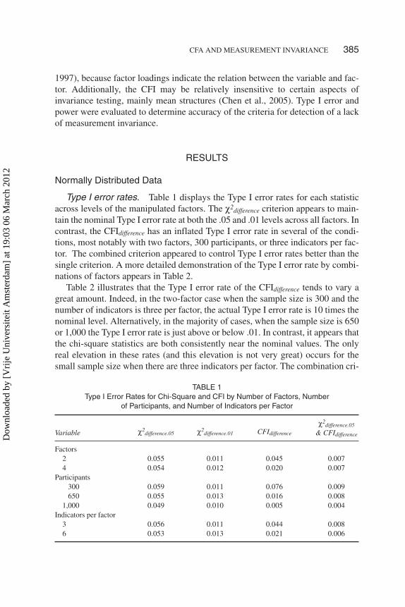
Type I error rates. Table 1 displays the Type I error rates for each statisticacross levels of the manipulated factors. The χ2difference criterion appears to main-tain the nominal Type I error rate at both the .05 and .01 levels across all factors. Incontrast, the CFIdifference has an inflated Type I error rate in several of the condi-tions, most notably with two factors, 300 participants, or three indicators per fac-tor. The combined criterion appeared to control Type I error rates better than thesingle criterion. A more detailed demonstration of the Type I error rate by combi-nations of factors appears in Table 2.

Table 2 illustrates that the Type I error rate of the CFIdifference tends to vary agreat amount. Indeed, in the two-factor case when the sample size is 300 and thenumber of indicators is three per factor, the actual Type I error rate is 10 times thenominal level. Alternatively, in the majority of cases, when the sample size is 650or 1,000 the Type I error rate is just above or below .01. In contrast, it appears thatthe chi-square statistics are both consistently near the nominal values. The onlyreal elevation in these rates (and this elevation is not very great) occurs for thesmall sample size when there are three indicators per factor. The combination cri-


TABLE 1Type I Error Rates for Chi-Square and CFI by Number of Factors, Number

of Participants, and Number of Indicators per Factor

Variable χ2difference.05 χ2

difference.01 CFIdifference

χ2difference.05

& CFIdifference

Factors2 0.055 0.011 0.045 0.0074 0.054 0.012 0.020 0.007

Participants300 0.059 0.011 0.076 0.009650 0.055 0.013 0.016 0.008

1,000 0.049 0.010 0.005 0.004Indicators per factor

3 0.056 0.011 0.044 0.0086 0.053 0.013 0.021 0.006

Dow

nloa

ded

by [

Vri

je U

nive

rsite

it A

mst

erda

m]

at 1

9:03

06

Mar

ch 2

012

terion, on average, resulted in lower Type I errors than the χ2difference and the CFIdif-

ference criteria when used alone.To examine the effects of the manipulated factors on the error rates, a variance

components analysis was conducted treating the error rates for each criterion as thedependent variable and the manipulated factors as the independent variables. Thisanalysis allows for an examination of the proportion of variance in the dependentvariable accounted for by the manipulated factors. Percentages above 10% are re-ported. Results indicate that for both χ2difference statistics the interaction of numberof factors, indicators per factor, and sample size accounted for more than 65% ofthe variation in Type I error rates, and approximately 20% was accounted for bythe total sample size main effect for both test statistics. In the case of the CFIdiffer-

ence, approximately 91% of variance in the Type I error rate was due to the samplesize. For the combination of CFIdifference and χ2difference , the interaction of the num-ber of indicators per factor by number of factors by sample size (73%) and thenumber of indicators per factor (12%) accounted for 85% of the variation in Type Ierror.

Power rates. Power by the levels of each factor appear in Table 3. As ex-pected, given the χ2difference.05 higher nominal Type I error rate, the χ2difference.05 cri-terion had higher power compared to the other criteria. For both chi-square differ-ence statistics, higher power is associated with a greater number of (a) factors, (b)participants, (c) indicators per factor, and (d) contaminated loadings. In contrast,the power of the CFIdifference test was higher with fewer factors and a smaller sam-


TABLE 2Type I Error by Number of Factors (F), Participants (N),

and Number of Indicators per Factor (I)

F N I χ2difference.05 χ2


χ2difference.05

& CFIdifference

2 300 3 0.070 0.010 0.130 0.0096 0.051 0.007 0.070 0.005

650 3 0.049 0.012 0.037 0.0106 0.055 0.015 0.014 0.013

1,000 3 0.048 0.008 0.016 0.0056 0.054 0.013 0.002 0.002

4 300 3 0.060 0.011 0.067 0.0086 0.056 0.017 0.036 0.015

650 3 0.063 0.014 0.013 0.0086 0.053 0.012 0.001 0.001

1,000 3 0.045 0.008 0.0 0.06 0.049 0.011 0.0 0.0

Dow

nloa

ded

by [

Vri

je U

nive

rsite

it A

mst

erda

m]

at 1

9:03

06

Mar

ch 2

012

ple size. In fact, the CFIdifference power was greatest in the high contamination con-dition and smallest sample size condition. The use of both the CFIdifference and theχ2difference results in lower power than for either individually. Indeed, at best, thepower of the combined criterion is constrained to be no higher than the power ofthe least powerful individual criterion. Recall that the CFIdifference had a higher TypeI error rate in the same conditions in which it exhibited higher power, suggestingthat the power results may not be very useful under certain conditions.

The levels of power by the four manipulated variables appear in Table 4. Again,when interpreting these results, it should be noted that the Type I error rate for theCFIdifference was somewhat elevated in a number of conditions. That is, power mightappear to be occasionally adequate, but at the expense of the loss of control of TypeI error. Nonetheless, it was within appropriate bounds frequently enough that anexamination of these more detailed results for power is warranted.

The variance components analysis for both χ2difference tests (results for theχ2difference.01 appear later, as χ2difference.05 results were nearly identical) shows thatapproximately 80% of the variation in power can be accounted for by five of themanipulated factors (or combinations of them), including the four-way Number ofFactors × Indicators Per Factor × Sample Size × Contamination interaction (21%),the three-way Number of Factors × Indicators Per Factor × Contamination interac-tion (12%), the two-way Sample Size × Level of Contamination interaction (11%),and the main effects of sample size (15%) and indicators per factor (21%). On theother hand, 78% of the variance in the power of the CFIdifference is accounted for bythe Number of Factors × Indicators Per Factor × Sample Size × Contamination in-


TABLE 3Power for Chi-Square and CFI by Number of Factors, Number of

Participants, Number of Indicators per Factor, and Level of Contamination

Variable χ2difference .05 χ2

difference .01 CFIdifference

χ2difference .05

& CFIdifference

Factors2 0.628 0.453 0.487 0.3804 0.748 0.597 0.374 0.333

Participants300 0.570 0.387 0.555 0.368650 0.612 0.425 0.275 0.247


3 0.586 0.387 0.386 0.2816 0.790 0.662 0.475 0.432

ContaminationHigh 0.781 0.635 0.560 0.481Low 0.595 0.415 0.301 0.232

Dow

nloa

ded

by [

Vri

je U

nive

rsite

it A

mst

erda

m]

at 1

9:03

06

Mar

ch 2

012

teraction (21%), the Number of Factors × Indicators Per Factor × Contaminationinteraction (25%), the Sample Size × Contamination interaction (17%), and themain effect of contamination (14%). For the combination of CFIdifference and theχ2difference, six terms accounted for 95% of the variance. These include the four-waySample Size × Number of Factors × Indicators Per Factor × Contamination inter-action (18%), the three-way Number of Factors × Indicators Per Factor × Contami-nation interaction (22%), the three-way Number of Factors × Indicators Per Factor× Sample Size interaction (13%), the two-way Sample Size × Contamination inter-action (18%), and the main effects of contamination (12%) and indicators per fac-tor (12%).

In general, for all three criteria, power is greater when the level of contamina-tion is high, sample size is large, and there are more indicators per factor. This lat-ter result is not universal, however. For instance, the power of the CFIdifference de-clines in the low contamination condition when the number of indicators per factor


TABLE 4Power by Number of Factors (F), Participants (N), Number of Indicators

per Factor (I), and Level of Contamination (C)

F N I C χ2difference.05 χ2


χ2difference.05

& CFIdifference

2 300 3 High 0.605 0.360 0.658 0.349Low 0.342 0.146 0.416 0.142

6 High 0.787 0.590 0.830 0.589Low 0.293 0.124 0.295 0.108

650 3 High 0.513 0.293 0.363 0.254Low 0.291 0.121 0.214 0.102

6 High 0.955 0.863 0.752 0.750Low 0.459 0.237 0.146 0.145

1,000 3 High 0.866 0.706 0.633 0.616Low 0.573 0.325 0.293 0.257

6 High 1.000 1.000 0.983 0.983Low 0.852 0.674 0.263 0.263

4 300 3 High 0.530 0.280 0.475 0.249Low 0.295 0.115 0.268 0.092

6 High 0.998 0.990 0.974 0.969Low 0.710 0.487 0.527 0.446

650 3 High 0.765 0.528 0.337 0.336Low 0.442 0.234 0.146 0.142

6 High 0.907 0.780 0.217 0.217Low 0.561 0.342 0.027 0.027

1,000 3 High 0.992 0.951 0.618 0.618Low 0.815 0.589 0.215 0.215

6 High 1.000 0.994 0.569 0.569Low 0.956 0.868 0.112 0.112

Dow

nloa

ded

by [

Vri

je U

nive

rsite

it A

mst

erda

m]

at 1

9:03

06

Mar

ch 2

012

increases from three to six, except when there are four factors and 300 participants.In addition, power for CFIdifference is not generally higher with four factors. Alterna-tively, for both chi-square difference tests, power is greater with four compared totwo factors, except with N = 300 and three indicators per factor.

In terms of comparative power among the three criteria, as might be expectedwhen alpha was higher, the χ2difference.05 had higher power than the other two crite-ria. When comparing the χ2difference.01 and the CFIdifference, it appears that CFIdifference

has higher power when the total sample size is 300 (corresponded to when its TypeI error rate was highly inflated), but that in most, but not all, other cases, thechi-square statistic has equivalent or higher power. This advantage for the χ2differ-

ence.01 is more marked in the four-factor case, particularly with larger samples andmore indicators per factor. Under select conditions, the power of the twochi-square statistics is very similar, suggesting that when the proportion of load-ings exhibiting group differences is sufficiently large, the alpha used may be im-material in terms of power. Specifically, when there are 1,000 participants, fourfactors, and six indicators per factor, the two criteria have essentially equivalentpower. A similar result is evident when there are four factors, six indicators per fac-tor, a sample size of 300, and a high level of contamination, or when there are 1,000participants, four factors, three indicators per factor, and a high level of contamina-tion. One final comparative difference in power to note is that for the smallest sam-ple size condition, coupled with two factors, the power of the CFIdifference is actuallyhigher than that of χ2difference.05. However, it is important to note that in general,with 300 participants, the Type I error rate of the CFIdifference is above the .05 levelof this chi-square criterion. Therefore, these results for CFIdifference must be inter-preted with caution, as the higher power comes with the price of an artificially ele-vated Type I error rate.

Power for testing a single loading. In addition to identifying a lack of in-variance among a set of factor loadings, power for detecting group differences onan individual loading was examined. This evaluation in practice would follow aninitial determination of a lack of invariance in the lambda matrix, and involvestesting each factor loading separately to determine where exactly this lack ofinvariance occurs. Therefore, contamination conditions remain as they were in theanalysis described previously, although only one of the contaminated loadings istested in this second stage of analysis. That is, power represents the detection of alack of invariance when only one loading simulated to be different was constrainedacross groups while the other loadings were freely estimated. The same criteriawere used to examine a single indicator as were used with testing the entire matrix.Table 5 displays the power for detecting lack of invariance for an individual load-ing by the manipulated factors.

The power of the χ2difference.05 to identify an individual loading is uniformlyhigher compared to the other criteria, which might be expected given its nominally


Dow

nloa

ded

by [

Vri

je U

nive

rsite

it A

mst

erda

m]

at 1

9:03

06

Mar

ch 2

012

(but only sometimes) larger alpha value. The χ2difference.01 had higher power thanthe CFIdifference in all cases. Finally, for all three criteria, the ability to detect the dif-ference for a single loading is lower than the ability to find differences for an entireset of loadings.

For all criteria, the power to detect group differences for an individual loading issomewhat lower for four factors as opposed to two for the χ2difference.05 and theCFIdifference, but not for the χ2difference.01. In addition, power is lower when there aremore indicators per factor, regardless of the level of contamination. Power for theχ2difference.05 is lower for the low contamination condition compared to high con-tamination, whereas the other two criteria had slightly higher power in the lowcontamination condition. Finally, it appears that power for all three criteria is high-est when the sample size is 1,000, but some differences exist for the other twosample size conditions. For instance, for the χ2difference.05 power is not greatly dif-ferent for sample sizes of 300 and 650. However, both CFIdifference and χ2difference.01

actually had a decline in power from 300 to 650, before increasing with 1,000.Table 6 provides more detailed results for each criterion by the combination of

the manipulated variables. Perhaps most striking in Table 6 is the number of casesin which the CFIdifference (and by extension the combination criteria) does not detectthe group difference for a single indicator. This result is particularly prevalentwhen there are four factors. Indeed, despite the fact that the CFIdifference has compa-rable power to the χ2difference.01 for some conditions when detecting overall groupdifferences, the criteria rarely performs as well for a single indicator. A second in-teresting result is that power for all criteria is much lower when detecting differ-ences for an individual indicator versus the set of indicators. For both chi-square


TABLE 5Power for Detecting Group Difference of a Single Indicator Loading

Variable χ2difference.05 χ2


χ2difference.05

& CFIdifference

Factors2 0.382 0.221 0.153 0.1274 0.323 0.235 0.012 0.011

Participants300 0.269 0.230 0.131 0.094650 0.276 0.125 0.043 0.041


3 0.412 0.252 0.160 0.1346 0.293 0.204 0.005 0.005

ContaminationHigh 0.403 0.216 0.069 0.056Low 0.302 0.240 0.096 0.082

Dow

nloa

ded

by [

Vri

je U

nive

rsite

it A

mst

erda

m]

at 1

9:03

06

Mar

ch 2

012

tests, there is greater power in the low contamination case for the two-factor mod-els when there are three indicators per factor. On the other hand, when there arefour factors, power is typically higher when the indicators exhibit greater contami-nation. However, with the two larger sample size conditions with six indicators perfactor this does not occur. These results were somewhat unexpected given the as-sumption that greater contamination would be associated with higher power, re-gardless of the levels of the other manipulated variables. The outcome suggeststhat to detect a group difference in factor loadings when more loadings differ mayactually be more difficult.

The variance components analysis indicated that for χ2difference.05, four terms ac-counted for 89% of the observed variation in power, including the three-way Con-tamination × Indicators Per Factor × Number of Factors interaction (53%), thetwo-way Indicators Per Factor × Number of Factors interaction (12%), contamina-


TABLE 6Power for Detecting Single Item Difference by Number of Factors (F),

Participants (N), Number of Indicators per Factor (I), and Levelof Contamination (C)

F N I C χ2difference.05 χ2


χ2difference.05

& CFIdifference

2 300 3 High 0.290 0.119 0.239 0.099Low 0.798 0.575 0.661 0.506

6 High 0.208 0.073 0.040 0.040Low 0.062 0.012 0.005 0.005

650 3 High 0.405 0.196 0.147 0.143Low 0.460 0.234 0.174 0.163

6 High 0.208 0.079 0.001 0.001Low 0.066 0.015 0.0 0.0

1,000 3 High 0.715 0.498 0.271 0.271Low 0.775 0.567 0.293 0.293

6 High 0.519 0.265 0.001 0.001Low 0.077 0.013 0.0 0.0

4 300 3 High 0.274 0.115 0.081 0.079Low 0.054 0.017 0.011 0.011

6 High 0.242 0.091 0.004 0.004Low 0.222 0.084 0.04 0.004

650 3 High 0.398 0.206 0.022 0.022Low 0.048 0.011 0.0 0.0

6 High 0.283 0.102 0.0 0.0Low 0.340 0.155 0.0 0.0

1,000 3 High 0.678 0.470 0.017 0.017Low 0.054 0.013 0.0 0.0

6 High 0.616 0.375 0.0 0.0Low 0.668 0.428 0.0 0.0

Dow

nloa

ded

by [

Vri

je U

nive

rsite

it A

mst

erda

m]

at 1

9:03

06

Mar

ch 2

012

tion (14%), and sample size (10%). Results for the χ2difference.01 also are presentedas they differed from the χ2difference.05. For χ2difference.01, three terms accounted for83% of the variance in power: the four-way Sample Size × Contamination × Indi-cators Per Factor × Number of Factors interaction (19%), the three-way Contami-nation × Indicators Per Factor × Number of Factors interaction (47%), and thetwo-way Sample Size × Contamination interaction (17%). For the CFIdifference,75% of the variance in power was accounted for by the Sample Size × Contamina-tion × Indicators Per Factor × Number of Factors interaction (29%) and the Indica-tors Per Factor × Number of Factors interaction (46%). Finally, 82% of the vari-ance in power for the combination criterion of the CFIdifference and the χ2difference wasaccounted for by the Sample Size × Contamination × Indicators Per Factor × Num-ber of Factors interaction (32%), the Indicators Per Factor × Number of Factors in-teraction (39%), and the number of indicators per factor (11%).

Dichotomous Data

Type I error rates. Based on the results for the ML estimation with normallydistributed data, described earlier, we decided not to use the CFIdifference or the com-bination criteria for determining a lack of invariance with the RWLS estimation.We should note that a few conditions where power was highest for CFIdifference inthe normal case were examined for power with dichotomous data using RWLS es-timation. Specifically, the power of CFIdifference with four factors, three indicatorsper factor, 1,000 participants, and high contamination was .0457, whereas powerwith four factors, six indicators per factor, 300 participants, and low contaminationwas 0. Finally, the power of CFIdifference with four factors, six indicators per factor,1,000 participants, and high contamination was .1537. As expected, in all threecases power was much lower for dichotomous data than in the normal case, sup-porting our reasoning for not including these two criteria in the remaining analy-ses. Thus, in the remaining results, only the χ2difference.05 is used. The Type I errorrate for the RWLS by the number of factors, participants, and items per factor ap-pears in Table 7.

The Type I error rate for the chi-square difference test with the RWLS estima-tion method is near the nominal rate regardless of the number of factors present inthe model or the number of items per factor. However, the number of participantsin the sample does seem to have a substantial impact on the error rate. With a totalsample size of 1,000, the Type I error rate is somewhat inflated above the nominal.05 level, whereas with 300 participants, the error rate is below the nominal level.This result stands in contrast to the normal case, where the sample size had a rathersmall influence on the Type I error rate. A more detailed display of the Type I errorrate by the manipulated variables appears in Table 8.

Perhaps the most revealing finding in Table 8 is that the impact of sample sizeon the Type I error rate is influenced, to some degree, by the number of items per


Dow

nloa

ded

by [

Vri

je U

nive

rsite

it A

mst

erda

m]

at 1

9:03

06

Mar

ch 2

012

factor. Variance components analysis for the Type I error rate indicates that ap-proximately 92% of the variance is due to the sample size. When there are feweritems (three), the error rate at all three sample sizes is somewhat higher than whenthere are more items, although this effect is most dramatic when sample size waslargest. Indeed, when there are four factors and six items per factor, the error ratewith 1,000 participants is only slightly above the nominal rate of .05. Additionally,


TABLE 7Type I Error Rates for Chi-Square for RobustWeighted Least Squares Difference Test byNumber of Factors, Number of Participants,

and Number of Items per Factor

Variable χ2difference.05

Factors2 0.0524 0.054

Participants300 0.028650 0.041

1,000 0.090Items per factor

3 0.0666 0.040

TABLE 8Type I Error Rate for Detecting Lack of Model Invariance for Robust

Weighted Least Squares Estimation by Number of Factors (F),Participants (N), Number of Items per Factor (I), and Level of

Contamination (C)

F N I χ2difference.05

NonconvergenceRate

2 300 3 0.031 0.4776 0.027 0.441

650 3 0.049 0.0916 0.022 0.180

1,000 3 0.111 0.0106 0.073 0.015

4 300 3 0.037 0.3106 0.016 0.568

650 3 0.053 0.0896 0.041 0.226

1,000 3 0.114 0.0106 0.060 0.026

Dow

nloa

ded

by [

Vri

je U

nive

rsite

it A

mst

erda

m]

at 1

9:03

06

Mar

ch 2

012

with 300 participants and six items per factor, regardless of the number of factors,the Type I error rate is noticeably lower than the nominal rate. In short, the impactof the number of participants on the Type I error rate is determined in part by thesize of the model being estimated, as expressed by the number of items per factor.

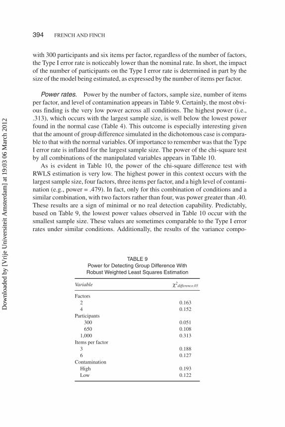
Power rates. Power by the number of factors, sample size, number of itemsper factor, and level of contamination appears in Table 9. Certainly, the most obvi-ous finding is the very low power across all conditions. The highest power (i.e.,.313), which occurs with the largest sample size, is well below the lowest powerfound in the normal case (Table 4). This outcome is especially interesting giventhat the amount of group difference simulated in the dichotomous case is compara-ble to that with the normal variables. Of importance to remember was that the TypeI error rate is inflated for the largest sample size. The power of the chi-square testby all combinations of the manipulated variables appears in Table 10.

As is evident in Table 10, the power of the chi-square difference test withRWLS estimation is very low. The highest power in this context occurs with thelargest sample size, four factors, three items per factor, and a high level of contami-nation (e.g., power = .479). In fact, only for this combination of conditions and asimilar combination, with two factors rather than four, was power greater than .40.These results are a sign of minimal or no real detection capability. Predictably,based on Table 9, the lowest power values observed in Table 10 occur with thesmallest sample size. These values are sometimes comparable to the Type I errorrates under similar conditions. Additionally, the results of the variance compo-


TABLE 9Power for Detecting Group Difference WithRobust Weighted Least Squares Estimation

Variable χ2difference.05

Factors2 0.1634 0.152

Participants300 0.051650 0.108

1,000 0.313Items per factor

3 0.1886 0.127

ContaminationHigh 0.193Low 0.122

Dow

nloa

ded

by [

Vri

je U

nive

rsite

it A

mst

erda

m]

at 1

9:03

06

Mar

ch 2

012

nents analysis show that 75% of the variance in power is accounted for by the sam-ple size.

Given these very low power values observed with RWLS estimation, coupledwith the result for the normal case (Tables 5 and 6) that suggests that the power fordetecting group differences for a single variable is lower than for detecting a lackof invariance across all variables, no further analyses were conducted with RWLS.The assumption is reasonable that the power for detecting differences for individ-ual items will be very low in most cases when RWLS estimation is used with di-chotomous data.

An additional issue pertinent to understanding the performance of the RWLSdifference testing is the rate of nonconvergence. Although this was a nonissue withthe ML estimation, the rates of nonconvergence for RWLS under certain condi-tions was very high. Examination of Tables 8 and 10 suggests that the problem is


TABLE 10Power of the Chi-square With Robust Weighted Least Squares Estimationby Number of Factors (F),Participants (N), Number of Items per Factor (I),

and Level of Contamination (C)

F N I C χ2difference.05

NonconvergenceRate

2 300 3 High 0.088 0.197Low 0.055 0.197

6 High 0.068 0.370Low 0.042 0.329

650 3 High 0.185 0.094Low 0.098 0.013

6 High 0.102 0.144Low 0.064 0.196

1,000 3 High 0.405 0.012Low 0.289 0.010

6 High 0.360 0.027Low 0.213 0.020

4 300 3 High 0.054 0.244Low 0.047 0.362

6 High 0.037 0.667Low 0.026 0.601

650 3 High 0.164 0.193Low 0.114 0.138

6 High 0.081 0.397Low 0.058 0.347

1,000 3 High 0.479 0.025Low 0.290 0.020

6 High 0.302 0.085Low 0.168 0.064

Dow

nloa

ded

by [

Vri

je U

nive

rsite

it A

mst

erda

m]

at 1

9:03

06

Mar

ch 2

012

particularly acute when the sample size is small and the model is more complex(larger numbers of items and factors). Indeed, the only factor that appears to guar-antee low rates of nonconvergence is a large sample. This lack of convergence isespecially problematic when there were 300 participants, where the rates wereabove 0.6 in some cases, and never below 0.2. Based on this result, it appears thatresearchers who want to use the RWLS difference testing with smaller samplesizes may run into serious problems in obtaining proper convergence and stable es-timates. Note that all Type I error rate and power results are based on a full set of1,000 replications. In cases where nonconvergence occurred, replacement sampleswere generated until 1,000 simulations were run for all conditions. Nonconver-gence rates were based on the first 1,000 replications run.

To better understand the relation between the performance of the χ2difference.05 andthe ability of the RWLS estimation procedure to converge, Pearson correlations be-tween convergence rates and both the Type I error and power were computed. In bothcases, the correlation was strong and negative (–.765 for Type I error and –.702 forpower). These results may indicate that the low power for detecting a lack ofinvariance associated with using RWLS estimation is due in part to difficulties forthe algorithm in correctly estimating parameters. Thus, even when convergence isachieved, the resulting estimates, in some cases, may not be stable. This instabilitymay overshadow any differences when the constrained and unconstrained modelsare compared. Clearly, regardless of the cause, testing for a lack of invariance suffersfrom low power with the use of RWLS for parameter estimation.

DISCUSSION

The results described suggest that when the indicator variables are normally dis-tributed and ML estimation is used, the χ2difference.05 test of invariance offers re-searchers generally good control of the Type I error rate, along with relatively highpower in most situations. Furthermore, the χ2difference.01 also adequately controlsthe Type I error rate, although, predictably, has lower power compared to the χ2dif-

ference.05. In contrast, the CFIdifference statistic behaved somewhat more erraticallythan the χ2difference.01 test. In cases where power comparisons between the CFIdiffer-

ence and the χ2difference.01 were possible due to noninflated Type I error rates, the lat-ter had higher power than the former. Using both criteria in conjunction yieldedvery low power, and did not appear to be a worthwhile alternative to either in isola-tion. As mentioned previously, power with a combination of criteria will be con-strained to the least powerful individual criterion, at best.

In terms of the factors that influence the Type I error rates of the criteria exam-ined, most important for the CFIdifference test appears to be sample size, where largersamples were associated with lower Type I error rates. Indeed, for samples of1,000, the rate is actually below .01. On the other hand, with samples of 300, the


Dow

nloa

ded

by [

Vri

je U

nive

rsite

it A

mst

erda

m]

at 1

9:03

06

Mar

ch 2

012

Type I error rate can be up to 10 times more than this rate. The CFIdifference test alsoappears to have subnominal Type I error rates in certain cases when there are sixvariables per factor. In contrast, none of the manipulated variables had a markedimpact on the error rates of either of the chi-square criteria. In sum, this findingsuggests that in some sense, this test is more stable than the CFIdifference, and that in-deed the chi-square tests are generally a dependable tool in terms of maintainingthe nominal Type I error rate in factorial invariance studies.

With respect to power, the primary variables influencing the chi-square criteriaare sample size and the number of indicators per factor. In general, the more partic-ipants included in the analysis, the greater the power for the chi-square differencetest, regardless of the nominal alpha. In addition, irrespective of the sample size,there is greater power for detecting a lack of invariance with more indicators perfactor. The number of factors has some impact on the power of both the chi-squaredifference test as well as the CFIdifference, although the nature of the effect is verydifferent. For both chi-square criteria, power was higher for models with four fac-tors than those with two, and conversely, the power of the CFIdifference was higher inthe two-factor than the four-factor case. The number of indicators per factor alsohas a noticeable impact on the power of CFIdifference, with more indicators associ-ated with higher power, as was seen with the chi-square statistics.

When differences in models have been detected between two groups, a re-searcher will naturally be interested in isolating the specific items or subtests thatdiffer across the groups. For this to be evaluated, the data analyst will need to con-duct model invariance tests for individual indicators by allowing each to be con-strained as others are free to vary across groups. The results of this simulationstudy suggest that for any of the statistics used here, power is much reduced whentesting invariance for a single indicator versus that of the entire set. The power ofthe CFIdifference test is particularly low when testing for invariance of a single indi-cator, although even the chi-square statistics suffer reductions in their ability to de-tect group differences. The only instance when the CFIdifference is more powerfulthan the χ2difference.01 is when the sample size is 300 and the model is simple (i.e.,three indicators per factor and two factors). However, note that this combination ofconditions is associated with an inflated Type I error rate in the testing of overallinvariance so that interpretation of power in this context is not meaningful. In con-trast, often with four factors the CFIdifference power for testing a single indicator wasactually zero.

The chi-square difference criteria also suffer from a diminution in power in thesingle indicator case, although not as severe as seen with the CFIdifference test. Addi-tionally, some of the effects of the manipulated variables when testing all of the indi-cators are reversed when examining an individual indicator. For example, when test-ing a single indicator, models of greater complexity (more factors and moreindicators) were actually associated with lower power, in contrast to the situationwhen testing all indicators. This result seems logical, in that with more indicators


Dow

nloa

ded

by [

Vri

je U

nive

rsite

it A

mst

erda

m]

at 1

9:03

06

Mar

ch 2

012

and more factors that presumably do not differ by group, the single indicator that dif-fers might be hidden in the crowd. This is in contrast to recent suggestions that it maybe easier to locate invariance when only a few variables lack invariance (Millsap,2005). On the other hand, as with testing the entire set of indicators, larger samplesizes are associated with greater power for the chi-square difference tests.

An interesting result present for all of the criteria examined is that power in thelow contamination condition was higher compared to the high contamination fortwo factors and three indicators per factor with samples of size 300 or 650 and forfour factors with six indicators per factor. In other words, power for detecting groupdifferences for a single item is greater when the number of items that actually differbetween the groups is smaller, in accord with Millsap (2005), if the problem itself issomewhat simpler (fewer factors and fewer participants). This outcome would sug-gest that when a researcher is interested in isolating individual indicator differences(or lack thereof), one must be aware of not only the individual target indicator, butalso the potential of group differences for other indicators in the set.

As noted earlier, recent work has found that for dichotomous items, RWLS ap-pears to be preferable in terms of estimating item parameters in the CFA context(Flora & Curran, 2004). Therefore, this approach was selected for testing modelinvariance with dichotomous items. The results presented here suggest that the TypeI error rate generally tended to be at or below the nominal .05 level, except when thesample size was 1,000 and the number of items per factor was small. Of greater con-cern in thiscontext thanTypeIerrorcontrol is thehighrateofnonconvergence incer-tain instances.Withsamplesof1,000, thisproblemoccurredvery infrequently;how-ever,when therewere300participants, nonconvergencewasnearlyascommon(andin one case more common) than convergence. Clearly, this result suggests that forcertain applications, researchers may have difficulty applying RWLS because themethod may not yield estimates due to small sample sizes.

The power of the RWLS chi-square test for testing invariance is very low incomparison with that for the normal data using ML estimation. In fact, in a numberof cases, power is nearly indistinguishable from the Type I error rate. Specifically,it is lowest for the smallest sample size, as was found with ML estimation. How-ever, even when the sample is 1,000, power never reaches .50, and is most often be-low .40. As with the ML estimation, power is somewhat lower for situations inwhich there are six indicators per factor, and for the lower level of contamination.Again, however, even in the best situations, power for the RWLS remains very lowrelative to the normally distributed variables with ML estimation.

CONCLUSIONS

The results of this study present several implications for the practitioner who plansto conduct factorial invariance analyses using either the ML or RWLS approaches


Dow

nloa

ded

by [

Vri

je U

nive

rsite

it A

mst

erda

m]

at 1

9:03

06

Mar

ch 2

012

for normally distributed or dichotomous variables, respectively. First, when it isappropriate to use ML, the chi-square difference test maintains the nominal Type Ierror rate at both .05 and .01, across a variety of sample size and model complexityconditions. In addition, the chi-square difference test provides comparable orbetter power than the CFIdifference test, whereas the latter does have some inflationof the Type I error rate for small sample sizes. In short, the chi-square differencetest appears to be a solid candidate for testing model invariance in the ML case, andmay be more appropriate in many cases than the CFIdifference test.

Second, although the chi-square test for overall lack of invariance appears to of-fer satisfactory power in many instances, the same cannot be said of the tests for in-dividual indicators. In most applied situations, a researcher will need to follow up asignificant overall test for a lack of invariance with tests of the individual indica-tors to isolate where differences occur. However, the results presented in this studyseem to suggest that the power for such tests might often be fairly low. Perhapsmost surprising is that even in some cases where N is 1,000, the power is below .20.The incidence of low power is exacerbated by a more complex model structure(more variables and more factors). This result could potentially present the practi-tioner with the conundrum of having sufficient power to detect an overall differ-ence between groups but not having the power to find such differences for individ-ual indicators. Such an outcome could lead to the unsatisfying conclusion thatthere is a difference in factor loadings between the groups somewhere, but it is notpossible to say where.

A third major implication of this study is that power appears to be a major prob-lem for the chi-square difference test when the RWLS method of estimation is em-ployed. Indeed, the possibility exists that power would be nearly as low as the TypeI error rate with small sample sizes. Certainly, in practice, having such a low proba-bility of detecting group differences in terms of factor loadings hampers the abilityof a researcher to make substantive statements about invariance. Based on the re-sults presented, it would seem that only in the largest sample size condition is it re-alistic for researchers to expect to find differences between groups when theyshould find them. For many applied researchers, this could suggest limited utilityin applying the chi-square difference test when RWLS estimation is used becauseobtaining such large samples is often not feasible, especially with low-incidencepopulations. A separate but related problem to that of power in the RWLS case isthe fairly high rate of nonconvergence when sample sizes are small. Although thisproblem did not appear to be severe with 1,000 participants, it was increasinglylikely to occur when only 300 participants were available. Again, for many studies,obtaining as many as 1,000 participants is not possible, making the application ofthe preferred method of estimation, RWLS, in group invariance testing lessfeasible.

The purpose of this investigation is to provide evidence of MCFA performancefor measurement invariance testing under a variety of practical and applied condi-


Dow

nloa

ded

by [

Vri

je U

nive

rsite

it A

mst

erda

m]

at 1

9:03

06

Mar

ch 2

012

tions. However, although several thousand samples were examined, simulation ofexhaustive conditions is not practically possible. For instance, an important aspectof this study to recall is that properly specified baseline models were simulated.Results cannot be assumed to apply to situations when baseline models do notmeet this condition. That is, results of this study are dependent on properly speci-fied baseline models. Additionally, the sample size of 650 deserves further explo-ration as it may represent effects of uneven sample sizes and not just a moderate to-tal sample size. Therefore, further simulation work is encouraged to continue toexamine MCFA analyses under various additional conditions (e.g., referent indica-tor, longitudinal data, etc.) as there are several problems that remain to be solved ininvariance testing (Millsap, 2005). That said, this research should inform practicefor those using model invariance analyses to better understand phenomena in theirdisciplines. The results described here should (a) allow practitioners to make in-formed decisions about the use of GFIs to determine measurement invariance, (b)inform practice by highlighting the strengths and limitations of MCFA given cer-tain conditions (e.g., complex models, nonnormality), and (c) stimulate new re-search surrounding the implementation of the MCFA. For example, it is clear that ameasure of effect size would be very helpful in allowing power results to be moremeaningfully examined (Cheung & Rensvold, 2002; Millsap, 2005).

Continued examination of methods, such as MCFA, for gathering score validityevidence is crucial in many fields. Practitioners rely on methodologies such asthese to compare instruments across groups, thus ensuring that constructs, and ulti-mately test scores, have equal meaning and interpretation for a variety of individu-als. Knowledge of when such methods have difficulties in comparing groups is es-sential so that conclusions about group differences (or lack of differences) can beinterpreted accurately. Results presented here would suggest that when ML is usedfor normally distributed indicators, the MCFA approach using chi-square differ-ence tests will often yield reasonable outcomes regarding group invariance overall,but may have difficulties in pinpointing differences for individual factor loadings.Furthermore, when RWLS is used with dichotomous items, care must be taken inthe interpretation of findings suggesting that group invariance holds, particularlyfor smaller sample sizes, in light of the low power results and nonconvergencerates.

REFERENCES

Alwin, D. F., & Jackson, D. J. (1981). Applications of simultaneous factor analysis to issues of factorialinvariance. In D. Jackson & E. Borgatta (Eds.), Factor analysis and measurement in sociological re-search: A multi-dimensional perspective (pp. 249–279). Beverly Hills, CA: Sage.

American Educational Research Association, American Psychological Association, & National Coun-cil on Measurement in Education. (1999). Standards for educational and psychological testing.Washington, DC: American Educational Research Association.


Dow

nloa

ded

by [

Vri

je U

nive

rsite

it A

mst

erda

m]

at 1

9:03

06

Mar

ch 2

012

Bollen, K. A. (1989). Structural equations with latent variables. New York: Wiley.Bollen, K. A. (1990). Overall fit in covariance structure models: Two types of sample size effects. Psy-

chological Bulletin, 107, 256–259.Brannick, M. T. (1995). Critical comments on applying covariance structure modeling. Journal of Or-

ganizational Behavior, 16, 201–213.Brennan, R. L. (2004). Revolutions and evolutions in current educational testing (CASMA Research

Rep. No. 4). Iowa City: University of Iowa.Byrne, B. M., Shavelson, R. J., & Muthén, B. O. (1989). Testing for the equivalence of factor

covariance and mean structures. Psychological Bulletin, 105, 456–466.Chen, F. F., Sousa, K. H., & West, S. G. (2005). Testing measurement invariance of second-order factor

models. Structural Equation Modeling, 12, 471–492.Cheung, G. W., & Rensvold, R. B. (1999). Testing factorial invariance across groups: A reconceptuali-

zation and proposed new method. Journal of Management, 25, 1–27.Cheung, G. W., & Rensvold, R. B. (2002). Evaluating goodness-of-fit indexes for testing measurement

invariance. Structural Equation Modeling, 9, 233–255.Flora, D. B., & Curran, P. J. (2004). An empirical evaluation of alternative methods of estimation for

confirmatory factor analysis with ordinal data. Psychological Methods, 9, 466–491.Haladyna, T. M., & Downing, S. M. (2004). Construct-irrelevant variance in high-stakes testing. Edu-

cational Measurement: Issues and Practice, 23, 17–27.Horn, J. L., & McArdle, J. J. (1992). A practical and theoretical guide to measurement invariance in ag-

ing research. Experimental Aging Research, 18, 117–144.Hu, L., & Bentler, P. M. (1998). Fit indices in covariance structure modeling: Sensitivity to under-

parameterized model misspecification. Psychological Methods, 1, 424–451.Jöreskog, K. G. (1971). Simultaneous factor analysis in several populations. Psychometrika, 57,

409–426.Jöreskog,K.G.,&Sörbom,D. (1996).LISREL8:User’sreferenceguide.Chicago:ScientificSoftware.Keith, T. Z. (1997). Using confirmatory factor analysis to aid in understanding the constructs measured

by intelligence tests. In D. P. Flanagan, J. L. Genshaft, & P. L. Harrison (Eds.), Contemporary intel-lectual assessment: Theories, tests, and issues (pp. 373–403). New York: Guilford.

Kelloway, E. K. (1995). Structural equation modeling in perspective. Journal of Organizational Behav-ior, 16, 215–224.

Little, T. D. (1997). Mean and covariance structures (MACS) analyses of cross-cultural data: Practicaland theoretical issues. Multivariate Behavioral Research, 31, 53–76.

Lord, F., & Novick, M. R. (1968). Statistical theories of mental test scores. Reading, MA: Addi-son-Wesley.

Lubke, G. H., & Muthén, B. O. (2004). Applying multigroup confirmatory factor models for continu-ous outcomes to Likert scale data complicates meaningful group comparisons. Structural EquationModeling, 11, 514–534.

MacCallum, R. C., Widaman, K. F., Zhang, S., & Hong, S. (1999). Sample size in factor analysis. Psy-chological Methods, 4, 84–99.

Maller, S. J., & French, B. F. (2004). Factor invariance of the UNIT across deaf and standardizationsamples. Educational and Psychological Measurement, 64, 647–660.

Mantzicopoulos, P. Y., French, B. F., & Maller, S. J. (2004). Factor structure of the pictorial scale of per-ceived competence and social acceptance with two pre-elementary samples. Child Development, 75,1214–1228.

McGaw, B., & Jöreskog, K. G. (1971). Factorial invariance of ability measures in groups differing in in-telligence and socio-economic status. British Journal of Mathematical and Statistical Psychology,24, 154–168.

Meade, A. W., & Lautenschlager, G. J. (2004). A Monte-Carlo study of confirmatory factor analytictests of measurement equivalence/invariance. Structural Equation Modeling, 11, 60–72.


Dow

nloa

ded

by [

Vri

je U

nive

rsite

it A

mst

erda

m]

at 1

9:03

06

Mar

ch 2

012

Meredith, W. (1993). Measurement invariance, factor analysis and factorial invariance. Psychometrika,58, 525–543.

Messick, S. (1989). Meaning and values in test validation. The science and ethics of assessment.Educational Researcher, 18, 5–11.

Millsap, R. E. (2005). Four unresolved problems in studies of factorial invariance. In A.Maydeu-Olivares & J. J. McArdle (Eds.), Contemporary psychometrics (pp. 153–172). Mahwah,NJ: Lawrence Erlbaum Associates, Inc.

Millsap, R. E., & Tein, J.-Y. (2004). Assessing factorial invariance in ordered-categorical measures.Multivariate Behavioral Research, 39, 479–515.

Muthén, B., du Toit, S. H. C., & Spisic, D. (1997). Robust inference using weighted least squares andquadratic estimating equations in latent variable modeling with categorical and continuous out-comes. Unpublished manuscript, UCLA.

Muthén, B., & Lehman, J. (1985). Multiple group IRT modeling: Applications to item bias analysis.Journal of Educational Statistics, 10, 133–142.

Muthén, L. K., & Muthén, B. O. (2004). Mplus user’s guide, version 3. Los Angeles: Author.Raju, N. S., Laffitte, L. J., & Byrne, B. M. (2002). Measurement equivalence: A comparison of methods

based on confirmatory factor analysis and item response theory. Journal of Applied Psychology, 87,517–529.

Rensvold, R. B., & Cheung, G. W. (1998). Testing measurement models for factorial invariance: A sys-tematic approach. Educational and Psychological Measurement, 58, 1017–1034.

Swaminathan, H., & Rogers, H. J. (1990). Detecting differential item functioning using logistic regres-sion procedures. Journal of Educational Measurement, 27, 361–370.

Sörbom, D. (1974). A general model for studying differences in factor means and factor structures be-tween groups. British Journal of Mathematical and Statistical Psychology, 27, 229–239.

Thissen, D., Steinberg, L., & Wainer, H. (1993). Detection of differential item functioning using the pa-rameters of item response models. In P. W. Holland & H. Wainer (Eds.), Differential item functioning(pp. 67–113). Hillsdale, NJ: Lawrence Erlbaum Associates, Inc.

Thurstone, L. L. (1947). Multiple factor analysis: A development and expansion of the vectors of themind. Chicago: University of Chicago Press.

Vandenberg, R. J. (2002). Toward a further understanding of and improvement in measurementinvariance methods and procedures. Organizational Research Methods, 5, 139–158.

Vandenberg, R. J., & Lance, C. E. (2000). A review and synthesis of the measurement invariance litera-ture: Suggestions, practices, and recommendations for organizational research. Organizational Re-search Methods, 3, 4–69.


Dow

nloa

ded

by [

Vri

je U

nive

rsite

it A

mst

erda

m]

at 1

9:03

06

Mar

ch 2

012

Confirmatory Factor Analytic Procedures for the...

Documents

Transcript of Confirmatory Factor Analytic Procedures for the...