Configuration of the MPC10x10 for Tennessee Eastman ...€¦ · thermodynamic and chemical...

http://support.automation.siemens.com/WW/view/en/101978659

Application description 10/2014

Configuration of the MPC10x10 for

Tennessee Eastman Benchmark

Process SIMATIC PCS 7 V8.1 / Model Predictive Controller 10x10


Warranty and liability

MPC10x10 Entry-ID: 101978659, V1.0, 10/2014 2

S

iem

ens

AG 2

014

All r

ight

s re

serv

ed

Warranty and liability

Note The Application Examples are not binding and do not claim to be complete regarding the circuits shown, equipping and any eventuality. The Application Examples do not represent customer-specific solutions. They are only intended to provide support for typical applications. You are responsible for ensuring that the described products are used correctly. These application examples do not relieve you of the responsibility to use safe practices in application, installation, operation and maintenance. When using these Application Examples, you recognize that we cannot be made liable for any damage/claims beyond the liability clause described. We reserve the right to make changes to these Application Examples at any time without prior notice. If there are any deviations between the recommendations provided in these application examples and other Siemens publications – e.g. Catalogs – the contents of the other documents have priority.

We do not accept any liability for the information contained in this document.

Any claims against us – based on whatever legal reason – resulting from the use of the examples, information, programs, engineering and performance data etc., described in this Application Example shall be excluded. Such an exclusion shall not apply in the case of mandatory liability, e.g. under the German Product Liability Act (“Produkthaftungsgesetz”), in case of intent, gross negligence, or injury of life, body or health, guarantee for the quality of a product, fraudulent concealment of a deficiency or breach of a condition which goes to the root of the contract (“wesentliche Vertragspflichten”). The damages for a breach of a substantial contractual obligation are, however, limited to the foreseeable damage, typical for the type of contract, except in the event of intent or gross negligence or injury to life, body or health. The above provisions do not imply a change of the burden of proof to your detriment. Any form of duplication or distribution of these Application Examples or excerpts hereof is prohibited without the expressed consent of Siemens Industry Sector.

Security informa-tion

Siemens provides products and solutions with industrial security functions that support the secure operation of plants, solutions, machines, equipment and/or networks. They are important components in a holistic industrial security concept. With this in mind, Siemens’ products and solutions undergo continuous development. Siemens recommends strongly that you regularly check for product updates.

For the secure operation of Siemens products and solutions, it is necessary to take suitable preventive action (e. g. cell protection concept) and integrate each component into a holistic, state-of-the-art industrial security concept. Third-party products that may be in use should also be considered. For more information about industrial security, visit http://www.siemens.com/industrialsecurity.

To stay informed about product updates as they occur, sign up for a product-specific newsletter. For more information, visit http://support.automation.siemens.com.

http://www.siemens.com/industrialsecurity

http://support.automation.siemens.com/

Table of contents

MPC10x10 Entry-ID: 101978659, V1.0, 10/2014 3

S

iem

ens

AG 2

014

All r

ight

s re

serv

ed

Preface Objective of the application

In addition to the model based predictive controller ModPreCon for up to 4x4 interacting manipulated and controlled variables the new large predictive controller MPC10x10 for up to 10x10 manipulated and controlled variables is introduced in the context of PCS 7 V8.1. The MPC10x10 not only offers larger variable numbers but also some principally new functions which are introduced in this application note. This document expands the applications notes "Model based predictive multi-variable control at the example of a distillation column" (Entry-ID: 37361208) and "Fluidized bed dryer - design of a predictive controller with operating point optimization" (Entry-ID: 61926069) in which the functions of the ModPreCon are already described and is focused on the new features of the MPC10x10. Using the example of a processing plant with several units (Tennessee Eastman benchmark process with reactor, separator, stripper and compressor) the design of the MPC10x10 as a supervisory master controller is explained, dealing with six manipulated variables, five controlled variables and three measurable disturbance variables.

Main contents of this application The following issues are treated in this application: • Identification of process models with numerous manipulated and controlled

variables • Dynamic online optimization considering constraints • Setting of target values for manipulated variables • Simulation studies inside MPC configurator • Commissioning and test of the controller

Validity SIMATIC PCS 7 V8.1

Table of contents

MPC10x10 Entry-ID: 101978659, V1.0, 10/2014 4

S

iem

ens

AG 2

014

All r

ight

s re

serv

ed

Table of contents Warranty and liability ................................................................................................... 2

Preface .......................................................................................................................... 3 1 Automation Task ................................................................................................ 5

1.1 Overview............................................................................................... 5 1.2 The Tennessee Eastman Process ....................................................... 6 1.3 Simulation Model .................................................................................. 7 1.4 Requirements for Control of the Tennessee Eastman Process ........... 8

2 Basic Automation ............................................................................................ 10

2.1 Basic Control Loops ........................................................................... 10 2.2 Process Units of the Overall Plant ..................................................... 12 2.2.1 Reactor ............................................................................................... 12 2.2.2 Condenser .......................................................................................... 13 2.2.3 Separator ............................................................................................ 14 2.2.4 Stripper ............................................................................................... 15 2.3 Safety Interlocks ................................................................................. 16

3 Control Structure of MPC10x10 ..................................................................... 17

3.1 Notes on Definition of Control Structure ............................................. 17 3.2 Controlled Variables, Manipulated- and Disturbance Variables......... 17 3.3 CPU Resources .................................................................................. 19 3.4 Connection in CFC ............................................................................. 20 3.5 SFC for Switchover to MPC ............................................................... 21 3.6 Task oriented OS Screen ................................................................... 21

4 MPC10x10 Configuration ................................................................................ 22

4.1 Recording of Learning Data ............................................................... 22 4.2 Prior Knowledge ................................................................................. 22 4.3 Down sampling ................................................................................... 24 4.4 Process Model .................................................................................... 25 4.5 CV Importance and MV Target Values .............................................. 27 4.6 Parameterization of MV Move Penalties ............................................ 29 4.7 Verifikation .......................................................................................... 30 4.8 Simulation ........................................................................................... 31 4.8.1 Parameterization of Simulation .......................................................... 31 4.8.2 Model Variations and Simulation Results ........................................... 33 4.8.3 Dynamic Online Optimization ............................................................. 36

5 Commissioning of the MPC10x10 in SIMATIC PCS 7 .................................. 38

5.1 Download of Configuration Data ........................................................ 38 5.2 Limits Checking .................................................................................. 38 5.3 Commissioning ................................................................................... 40 5.4 Controller Test .................................................................................... 42 5.4.1 Setpoint Steps .................................................................................... 42 5.4.2 Disturbance Scenarios ....................................................................... 49 5.4.3 Comparison of Simulation inside MPC Configurator to Real

Process (Rigorous Simulation Model) ................................................ 53 6 Benefit for Plant Operator Company ............................................................. 55

7 Related Literature ............................................................................................ 56

8 History............................................................................................................... 56

Appendix ..................................................................................................................... 57

1 Automation Task

MPC10x10 Entry-ID: 101978659, V1.0, 10/2014 5

S

iem

ens

AG 2

014

All r

ight

s re

serv

ed

1 Automation Task 1.1 Overview

Introduction This application note describes the design and simulation, the operation and test of the model predictive control block MPC10x10 using the example of the Tennessee Eastman benchmark process. The Tennessee Eastman benchmark is known in the worldwide control engineering community as a particularly ambitious control problem. The MPC10x10 is supposed to be the master controller of a cascade structure. As a supervisory controller for several units the MPC will take care of five controlled variables in this scenario. Six manipulated variables are available (setpoints of slave PID controllers inside the units) as well as the information of three measurable disturbance variables.

Overview of the Automation Task Figure 1-1 gives a summary of the automation task. Details are explained in the following sections. Figure 1-1: Task oriented operator screen of the overall plant

1 Automation Task

MPC10x10 Entry-ID: 101978659, V1.0, 10/2014 6

S

iem

ens

AG 2

014

All r

ight

s re

serv

ed

1.2 The Tennessee Eastman Process The Tennessee Eastman process is a benchmark control problem, which is described in detail by (Downs, 1993), and the process model is provided by the authors as a Fortran code. The process is based on a real chemical production method by Eastman Chemical Company, USA. The fundamental properties are described using material balances, energy balances and other physical, thermodynamic and chemical equations. The chemical plant consists of a reactor, a separator, a stripper1 and a compressor which drives a recycling circle. The P&I diagram is shown in Figure 1-2. Figure 1-2: P&I diagram of the Tennessee Eastman process

1 A stripper is a unit similar to a distillation column in which a component is removed from a liquid mixture with the help of a gas flow

1 Automation Task

MPC10x10 Entry-ID: 101978659, V1.0, 10/2014 7

S

iem

ens

AG 2

014

All r

ight

s re

serv

ed

Four educts A, C, E and D are fed to make two products and one byproduct by chemical reactions. An inert gas B is not involved in the reaction, but it must be considered for the solution of the problem. The reaction equations are:

𝐴(g) + 𝐶(g) + 𝐷(g) → 𝐺(liq) 𝐴(g) + 𝐶(g) + 𝐸(g) → 𝐻(liq) 𝐴(g) + 𝐸(g) → 𝐹(liq) 3𝐷(g) → 2𝐹(liq)

The gaseous educts A, D and E are fed into the reactor, where they react to form liquid products. The reactor has a liquid volume of 16.6 𝑚³ and the plant produces 14.3 𝑡 ℎ� .

The gaseous phase reactions are dependent on a nonvolatile catalyst which remains solved in the liquid phase of the reactor. The reaction rates depend on temperature according to an Arrhenius equation in which the first reaction is stronger temperature-dependent than the second. The products leave the reactor in vaporized form together with educts not yet reacted. The vapors are cooled in a condenser. After that steams and liquids are separated in a passive separator. Non condensed products are recirculated via a centrifugal compressor back into the reactor. The condensed contents are cleaned from remaining educts with the help of the educt stream C in the stripper. An inert gas B enters mainly with educt stream C, but also with streams D and A into the plant and leaves it combined with byproduct F via the purge valve of the separator. Educt A is supplied in a much smaller quantity than the educts C, D and E. The overall plant has more than 12 manipulated variables and 41 measured values. The manipulated variables are called XMV by Downs & Vogel, the measured values XMEAS. A list of manipulated and controlled variables can be found in the appendix as of Appendix.

1.3 Simulation Model The Fortran model of the Tennessee Eastman process was implemented in Matlab/Simulink and provided as a download by Arizona State University. The kernel function of the Simulink model is embedded into a Matlab framework and compiled. The data exchange between compiled Matlab model and PCS 7 runs via the OPC server of WinCC, achieving a cycle time of 500 ms. In relation to the simulation step size of 1 s this results in a time lapse i. e. the simulation is running twice as fast as real time. A handshake method is implemented such that the speed of simulation is oriented at the cycling time of the function block MatlabProxy in the PCS 7 controller. Although the simulation is running twice as fast as real time, a process transient takes a lot of time. Complete transient phenomena sometimes need 24 ℎ to be evaluated.

1 Automation Task

MPC10x10 Entry-ID: 101978659, V1.0, 10/2014 8

S

iem

ens

AG 2

014

All r

ight

s re

serv

ed

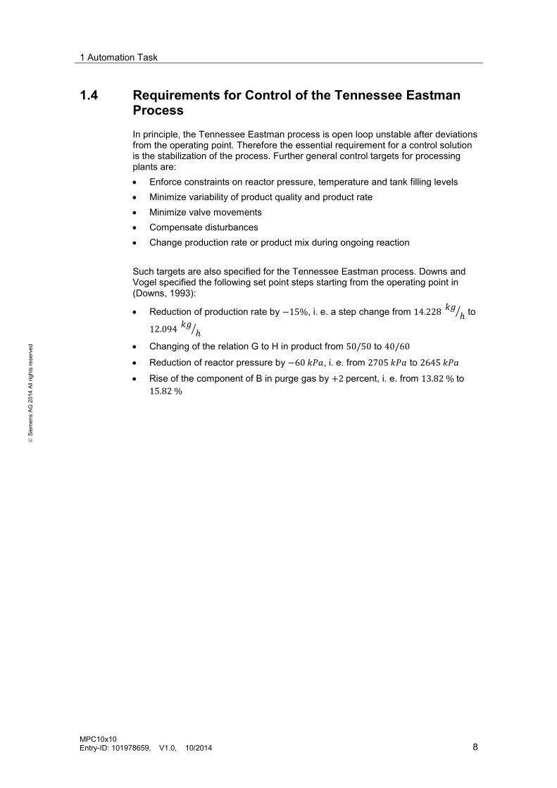
1.4 Requirements for Control of the Tennessee Eastman Process In principle, the Tennessee Eastman process is open loop unstable after deviations from the operating point. Therefore the essential requirement for a control solution is the stabilization of the process. Further general control targets for processing plants are: • Enforce constraints on reactor pressure, temperature and tank filling levels • Minimize variability of product quality and product rate • Minimize valve movements • Compensate disturbances • Change production rate or product mix during ongoing reaction

Such targets are also specified for the Tennessee Eastman process. Downs and Vogel specified the following set point steps starting from the operating point in (Downs, 1993):

• Reduction of production rate by −15%, i. e. a step change from 14.228 𝑘𝑔 ℎ� to

12.094 𝑘𝑔 ℎ�

• Changing of the relation G to H in product from 50/50 to 40/60

• Reduction of reactor pressure by −60 𝑘𝑃𝑎, i. e. from 2705 𝑘𝑃𝑎 to 2645 𝑘𝑃𝑎

• Rise of the component of B in purge gas by +2 percent, i. e. from 13.82 % to 15.82 %

1 Automation Task

MPC10x10 Entry-ID: 101978659, V1.0, 10/2014 9

S

iem

ens

AG 2

014

All r

ight

s re

serv

ed

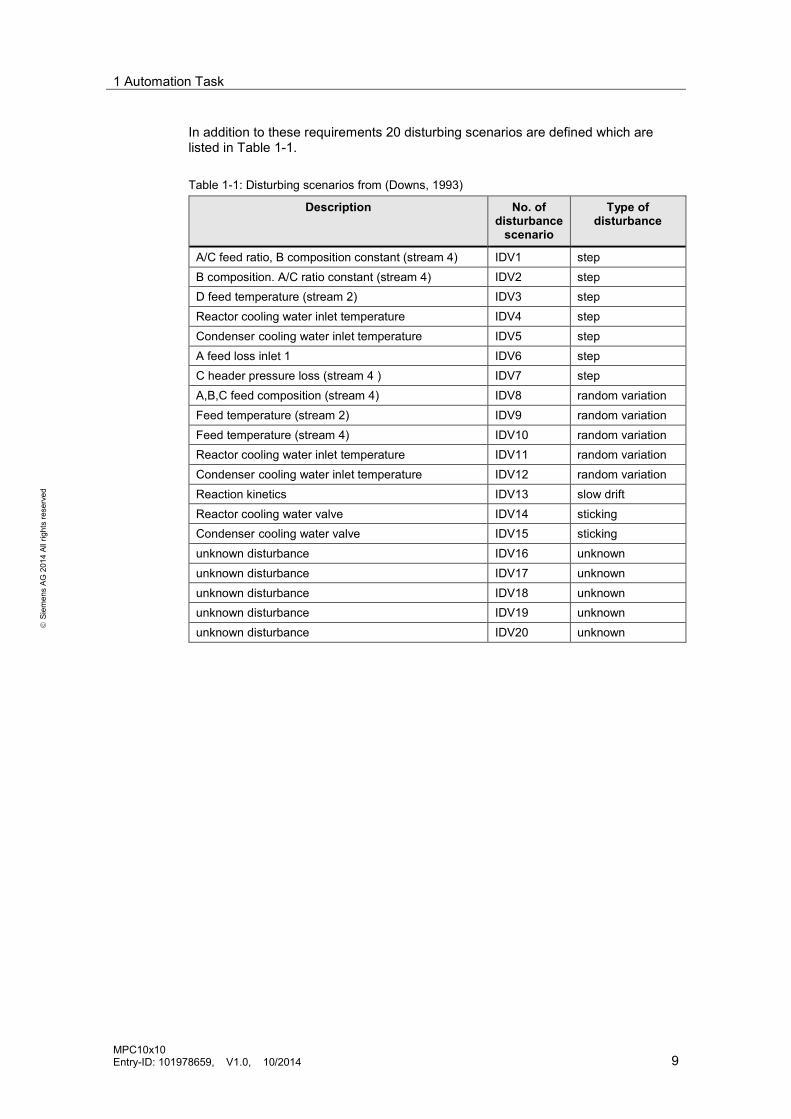
In addition to these requirements 20 disturbing scenarios are defined which are listed in Table 1-1. Table 1-1: Disturbing scenarios from (Downs, 1993)

Description No. of disturbance

scenario

Type of disturbance

A/C feed ratio, B composition constant (stream 4) IDV1 step B composition. A/C ratio constant (stream 4) IDV2 step D feed temperature (stream 2) IDV3 step Reactor cooling water inlet temperature IDV4 step Condenser cooling water inlet temperature IDV5 step A feed loss inlet 1 IDV6 step C header pressure loss (stream 4 ) IDV7 step A,B,C feed composition (stream 4) IDV8 random variation Feed temperature (stream 2) IDV9 random variation Feed temperature (stream 4) IDV10 random variation Reactor cooling water inlet temperature IDV11 random variation Condenser cooling water inlet temperature IDV12 random variation Reaction kinetics IDV13 slow drift Reactor cooling water valve IDV14 sticking Condenser cooling water valve IDV15 sticking unknown disturbance IDV16 unknown unknown disturbance IDV17 unknown unknown disturbance IDV18 unknown unknown disturbance IDV19 unknown unknown disturbance IDV20 unknown

2 Basic Automation

MPC10x10 Entry-ID: 101978659, V1.0, 10/2014 10

S

iem

ens

AG 2

014

All r

ight

s re

serv

ed

2 Basic Automation As already mentioned in chapter 1.4, the Tennessee Eastman process is unstable without a properly working base automation. The chemical reaction is strongly exothermic, i. e. it produces heat. In addition the speed of reaction increases with temperature, which results in positive feedback. Reactor pressure and temperature can rise strongly and fast, and at a certain point this can become irreversible. For safety reasons such a "thermal runaway" has to be absolutely avoided. Another reason for instability is an enrichment of inert gas B in the plant which leads to a rise in pressure. Pressure and temperature are coupled to each other in the gaseous phase by the general gas equation such that a rise in pressure also increases temperature and accordingly the speed of reaction. Some controlled systems show integrating behavior and are thus also unstable. This is typical for level control loops but integrating model behavior can also be found in temperature control loops if heat losses are neglected. In general, the recording of learning data for a model predictive controller requires a stable process behavior, which means that a base automation layer is indispensable for unstable processes. At first integrating controlled systems have to be stabilized by inserting P controllers in these cases.

2.1 Basic Control Loops

The design of basic automation is derived from approaches by (Ricker, 1995) which are slightly modified. The cascade control systems for pressure, compressor power, temperatures and filling levels are introduced briefly in the following.

Reactor Pressure Control Without basic control system the reactor pressure shows unstable behavior. Therefore a pressure controller PIC_Reactor is inserted, which passes its output as a set point to the flow controller FIC_Purge at the gas outlet of the separator. This defines the position of the purge valve which is opened at increasing pressure to remove non-reacted educts from there cycling loop.

Compressor Power Control To hold the compressor power approximately constant, a power controller JIC_Compressor is applied which uses the bypass valve as a manipulated variable. This control loop is operated with a large dead band since the compressor power just has to be kept in an area healthy for the compressor. An exact regulation of the compressor power is not required.

Reactor Temperature Control The reactor temperature controller TIC_Reactor provides its manipulated variable as a setpoint to the reactor cooling water temperature controller TIC_ReaCooling. The cooling water valve is available as manipulated variable for it. Both temperature control systems show integrating behavior. Therefore proportional-only controllers (without integral action) are used for stabilization.

Reactor Level Control The level in the reactor is kept approximately constant by the LIC_Reactor. This provides a set point to the temperature controller TIC_Separator, which is the master for the slave temperature controller TIC_Cooling in the condenser. This finally manipulates the process via the condenser cooling water valve.

2 Basic Automation

MPC10x10 Entry-ID: 101978659, V1.0, 10/2014 11

S

iem

ens

AG 2

014

All r

ight

s re

serv

ed

Stripper and Separator Level Control The levels of stripper and separator are controlled as usual: LIC_Separator and LIC_Stripper provide setpoints for the slave flow controllers FIC_Stripper and FIC_Separator that manipulate their respective outlet valves. Since the level processes are naturally integrating, the controllers are designed as proportional-only controllers.

Flow Controlof Educt Inlet Streams Flows of the inlet streams 1, 2, 3 and 4 are controlled with flow controllers FIC_EductA, FIC_EductD, FIC_EductE and FIC_EductC, which move the respective inlet valves.

2 Basic Automation

MPC10x10 Entry-ID: 101978659, V1.0, 10/2014 12

S

iem

ens

AG 2

014

All r

ight

s re

serv

ed

2.2 Process Units of the Overall Plant The overall plant consists of five separate process units (processing apparatus or machines) which are introduced in the following sections.

2.2.1 Reactor

The visualization of the reactor in the PCS 7 operator station with all reactor-related control loops is represented in Figure 2-1: P&I diagram of the reactor with the respective base control loops. Two controllers work across the unit borders: the level controler LIC_Reactor passes a setpoint to the temperature controller TIC_Separator in the separator, the pressure controller PIC_Reactor defines a setpoint for the flow controller FIC_Purge in the separator. In this unit the MPC10x10 block provides the external setpoints of following controllers: FIC_EductA, FIC_EductD, FIC_EductE, TIC_Reactor and PIC_Reactor. Gaseous products from the reactor are passed to the condenser. Figure 2-1: P&I diagram of the reactor with the respective base control loops

2 Basic Automation

MPC10x10 Entry-ID: 101978659, V1.0, 10/2014 13

S

iem

ens

AG 2

014

All r

ight

s re

serv

ed

2.2.2 Condenser

The condenser is visualized in the operator station like in Figure 2-2, in which there is only one controller, the temperature controller with an external setpoint from the temperature controller of the separator. The outlet of the condenser is connected to the separator. Figure 2-2: P&I diagram of the condenser with condensate temperature controller

2 Basic Automation

MPC10x10 Entry-ID: 101978659, V1.0, 10/2014 14

S

iem

ens

AG 2

014

All r

ight

s re

serv

ed

2.2.3 Separator

At the outlet of the separator in Figure 2-3 the gaseous flow is divided into two streams: One of these streams is a recycle flow to the reactor to reuse educts not yet reacted. The other flow serves to purge byproducts and primarily the inert gas B which can leave the circuit only this way. The liquid products are transferred to the stripper via the lower outlet of the separator. This flow is used to control the level in the separator at a constant value. Figure 2-3: P&I diagram of the separator with the related base control loops, the purge valve and exit to recirculation via compressor

2 Basic Automation

MPC10x10 Entry-ID: 101978659, V1.0, 10/2014 15

S

iem

ens

AG 2

014

All r

ight

s re

serv

ed

2.2.4 Stripper

The stripper shown in Figure 2-4 contains the controller FIC_EductC whose setpoint is a manipulated variable of the predictive controller. At the sump of the stripper the product leaves the considered part of the Tennessee Eastman process. At the head of the stripper low boiling components are removed and transferred to the reactor via the reflow. (Note that this connection is not shown for clarity reasons in the task oriented operator screen of the overall plant.) Figure 2-4: P&I diagram of the stripper with the related base control loops

2 Basic Automation

MPC10x10 Entry-ID: 101978659, V1.0, 10/2014 16

S

iem

ens

AG 2

014

All r

ight

s re

serv

ed

2.3 Safety Interlocks The usual interlocks in process plants prevent overflow or complete drain of tanks as well as the operation of pumps against closed valves. Furthermore in the Tennessee-Eastman process for safety reasons a "thermal runaway" of the reactor must be avoided in any case. If the chemical reaction "runs away", first the pressure and then the temperature rise steeply in the reactor and cannot be controlled any more with a standard control logic. In case of emergency a safety shutdown (trip) of the plant must be triggered. Besides the supervision of the absolute values of pressure and temperature it is reasonable to monitor the gradient of the pressure as well. A rising of the pressure too steeply is an early symptom for a “thermal runaway“ of the reactor. In the case of a safety shutdown all educt inlets are closed and the purge valve is opened.

3 Control Structure of MPC10x10

MPC10x10 Entry-ID: 101978659, V1.0, 10/2014 17

S

iem

ens

AG 2

014

All r

ight

s re

serv

ed

3 Control Structure of MPC10x10 3.1 Notes on Definition of Control Structure

As mentioned at the beginning, the MPC10x10 block is used as master controller in a cascade structure. For the Tennessee Eastman process the choice of controlled, manipulated and disturbance variables is not trivial. On the one hand, this is due to the unstable behavior of the process. On the other hand, the process shows strong interactions between different variables, even between different units. Because of these difficulties it is not obvious which process value has to be primarily influenced by which manipulated variable, since each variation of one manipulated variable also causes variations that must be accepted at another controlled variable. Another issue in context of definition of controller structure is the question which disturbance variables could have a significant influence on the controlled variables. If such disturbance variables are measurable, it is recommended to use them in the MPC as disturbance variables. In plants with a hierarchical control concept like the Tennessee Eastman process you should also check, whether there are underlaying control loops which could agitate independently because they are not part of the MPC cascade structure. Manipulated variable moves of independent control loops systems are also candidates for MPC disturbance variables.

3.2 Controlled Variables, Manipulated- and Disturbance Variables

In the following the controlled, manipulated and disturbance variables are described how they are used in the MPC10x10 block for the Tennessee Eastman problem. For the controlled and disturbance variables the variable names XMV und XMEAS from (Downs, 1993) are denoted, compare the details in the appendix as of page 57.

Controlled variables All substance concentrations are measured by analytical instruments and therefore they are provided only with a cycle time of 6 min or 15 min (plus dead time). Table 3-1: Controlled variables of large predictive controller

No. Controlled variable Unit Variable name

CV1 Production rate, flow at the stripper output m³h� XMEAS17

CV2 Concentration of component A at the reactor inlet mol% XMEAS23

CV3 Concentration of component E at the reactor inlet mol% XMEAS27

CV4 Concentration of component B in purge gas mol% XMEAS30

CV5 G in product, concentration of component G at the stripper output

mol% XMEAS40


MPC10x10 Entry-ID: 101978659, V1.0, 10/2014 18

S

iem

ens

AG 2

014

All r

ight

s re

serv

ed

Manipulated Variables Table 3-2: Manipulated variables of large predictive controller

No. Manipulated variables Unit

MV1 A feed, setpoint of FIC_EductA kscmh 2

MV2 D feed, setpoint of FIC_EductD kgh�

MV3 E feed, setpoint of FIC_EductE kgh�

MV4 C feed, setpoint of FIC_EductC kscmh MV5 Reactor pressure, setpoint of PIC_Reactor kPa

MV6 Reactor temperature, setpoint of TIC_Reactor °C

Disturbance Variables Table 3-3: Disturbance variables of large predictive controller

No. Disturbance variable Unit Variable name

DV1 Compressor reflux valve % XMV5 DV2 Reactor cooling water valve % XMV10 DV3 Stripper steam valve % XMV9

2 kscmh refers to the flow rate unit “kilo standard cubic meter per hour“


MPC10x10 Entry-ID: 101978659, V1.0, 10/2014 19

S

iem

ens

AG 2

014

All r

ight

s re

serv

ed

3.3 CPU Resources Please check the free memory space in the SIMATIC CPU before you load the MPC10x10 block into target system. The address range for function blocks (FB), functions without static local data (FC) and data blocks in SIMATIC Step 7 is restricted to 64 kByte (<16.000 real values) per block. A 10x10MPC with online optimization however needs several matrices with more than 100.000 elements altogether. The MPC algorithm is therefore split into a main function block MPC10x10 with faceplate and several auxiliary functions for dynamic optimization and static operating point optimization. The process model and further matrices required for the controller are distributed into up to 20 user data blocks. This complexity however is "hidden" away from the user: He only has to insert and link the main block MPC10x10 in CFC (Continuous Function Chart). The “look & feel" both in engineering and operator station is derived from the previous 4x4 ModPreCon function as far as possible. The memory space requirements for the MPC10x10and his auxiliary blocks can sum up to 850 Kbytes depending on quantity structure. Unlike the small ModPreCon only one single MPC10x10 can be accommodated in a SIMATIC CPU because of the address logic for the auxiliary blocks. Of course the calculation time is higher than for the small ModPreCon. Although controller cycle times of less than 5 s are feasible from a hardware point of view, an MPC for typical applications in processing plants will have considerably slower sample rates. The MPC is then called in the slowest cyclic task of the SIMATIC CPU (cycle time 20 s) and moreover works with an internal clock-pulse scaling. The base control loops and other automation functions are processed with higher priority in faster cyclic tasks and therefore they can interrupt the MPC calculations. Nevertheless you should make sure that the cycle load of the CPU is not close to the constraints before inserting the MPC10x10.


MPC10x10 Entry-ID: 101978659, V1.0, 10/2014 20

S

iem

ens

AG 2

014

All r

ight

s re

serv

ed

3.4 Connection in CFC The MPC10x10 must be linked correctly like any other block in the CFC. Because of the multitude of inputs and outputs the block needs more than one sheet in the CFC. Use the buttons "sheet view" and "overview" for the navigation, select a sheet via the accompanying drop down menu "sheet/overview" or use the key combination "Ctrl +arrow key”. Please configure at first the following inputs: • Connect CV and DV inputs to the appropriate process tags • Specify the operating point values for SP inputs • Specify reachable values for SP high and low limits • Specify the operating point values for MV manual inputs • Connect MV high and low limits for manual operating (MViManHi/LoLim) to SP

high and low limits of the slave controllers (in cascaded loops) or choose manipulated variable limits according to specifications of the respective actors (for direct access to the actors without cascaded slave controllers). The manipulated variable limits for automatic operation (MViHi/LoLim) are either set equal to the limits for manual or even to limiting values more narrow. A narrower limitation is recommended for example if stable closed loop control can be provided only in a restricted area around the operating point due to nonlinear process behavior

• Connect MV tracking inputs with SP outputs of slave controllers (for cascade loops) or with position feedback for direct access to the actor

• Connect MV TrackingOn with logical OR combination of CascadeCut outputs of slave controllers (or the valve block for direct access) and the output of the block AnyCV-Bad

• Connect MV Excite and ExciteOn inputs to the MV Excite and ExciteAct outputs of the AutoExcitation block if desired

• Specify manipulated variable targets for MV target inputs if desired. • Either specify CV and MV physical units directly or connect to PV_OutUnits of

process tags or slave controllers (for cascaded loops) • Connect Out-of-service inputs (OosLi) to OR combination of the

Out-of-Service outputs (OosAct) of the process tags In addition, you connect the MV outputs of the MPC10x10 block to the external setpoint inputs (SP_Ext) of the slave controllers (for cascaded loops) or to the inputs of the actor blocks (for direct access).

NOTE A cascade control scheme with an MPC master controller and several slave controllers is implemented according to the same principles of logical connection than a PID cascade, which are described in detail in the application note “Engineering of cascade control" / 5/.


MPC10x10 Entry-ID: 101978659, V1.0, 10/2014 21

S

iem

ens

AG 2

014

All r

ight

s re

serv

ed

3.5 SFC for Switchover to MPC

The sequence of steps for switchover from conventional control to MPC according to chapter 5.3 can be automated with a SFC if desired.

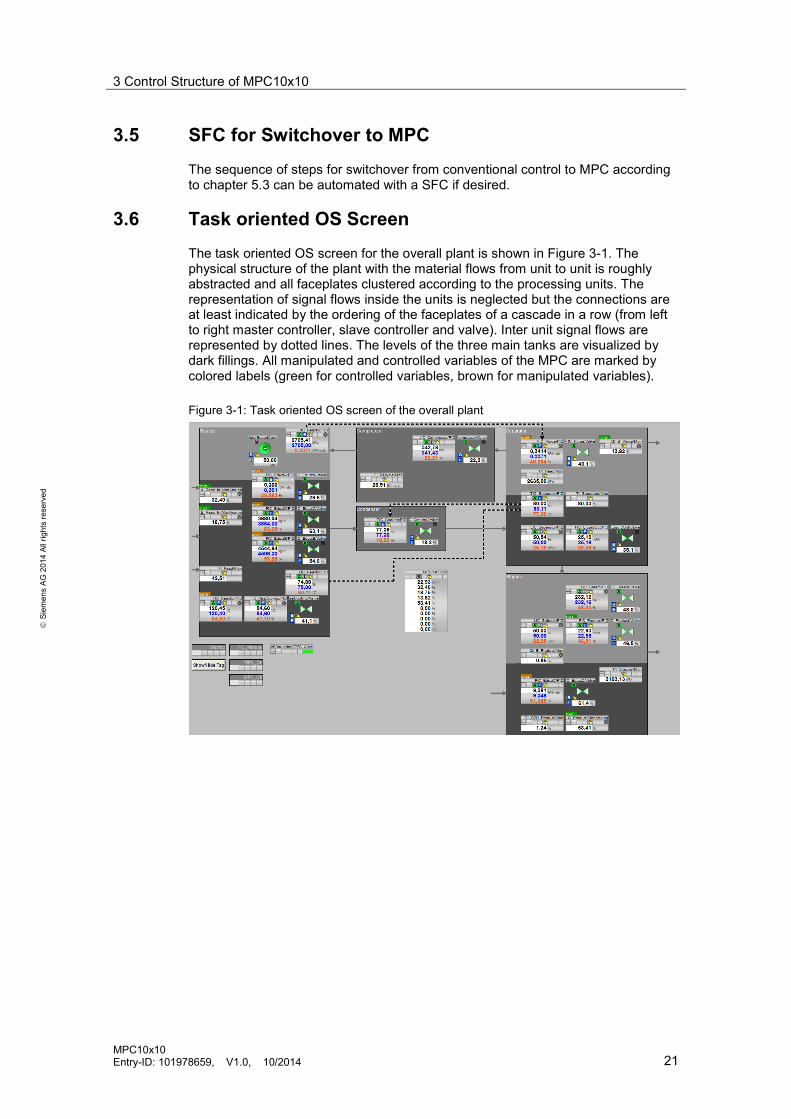
3.6 Task oriented OS Screen

The task oriented OS screen for the overall plant is shown in Figure 3-1. The physical structure of the plant with the material flows from unit to unit is roughly abstracted and all faceplates clustered according to the processing units. The representation of signal flows inside the units is neglected but the connections are at least indicated by the ordering of the faceplates of a cascade in a row (from left to right master controller, slave controller and valve). Inter unit signal flows are represented by dotted lines. The levels of the three main tanks are visualized by dark fillings. All manipulated and controlled variables of the MPC are marked by colored labels (green for controlled variables, brown for manipulated variables).

Figure 3-1: Task oriented OS screen of the overall plant

4 MPC10x10 Configuration

MPC10x10 Entry-ID: 101978659, V1.0, 10/2014 22

S

iem

ens

AG 2

014

All r

ight

s re

serv

ed

4 MPC10x10 Configuration 4.1 Recording of Learning Data

For the comfortable recording of learning data it is recommended to use the AutoExcitation block. Using this block you can pre-specify step sizes and step duration and do not need to operate the manual values successively by yourself. Before planning of learning data you should have assessed the settling times of the controlled variables. For the parameter specification of the AutoExcitation block the settling time of the controlled variable with the slowest response after a certain MV step is relevant. You will find further information on recording of learning data using AutoExcitation block in the application note "Fluidized bed dryer - design of a predictive controller with operating point optimization" (Entry-ID: 61926069).

4.2 Prior Knowledge

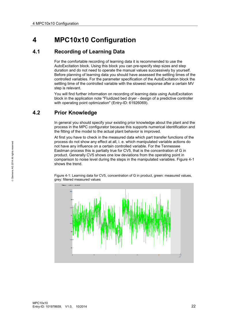
In general you should specify your existing prior knowledge about the plant and the process in the MPC configurator because this supports numerical identification and the fitting of the model to the actual plant behavior is improved. At first you have to check in the measured data which part transfer functions of the process do not show any effect at all, i. e. which manipulated variable actions do not have any influence on a certain controlled variable. For the Tennessee Eastman process this is partially true for CV5, that is the concentration of G in product. Generally CV5 shows one low deviations from the operating point in comparison to noise level during the steps in the manipulated variables. Figure 4-1 shows the trend. Figure 4-1: Learning data for CV5, concentration of G in product, green: measured values, grey: filtered measured values


MPC10x10 Entry-ID: 101978659, V1.0, 10/2014 23

S

iem

ens

AG 2

014

All r

ight

s re

serv

ed

The low signal-to-noise ratio visible here is a problem for model estimation, which results in low model precision for this channel after the identification. In this case this cannot be avoided since for larger steps of the manipulated variables the open control loop is unstable. If such a danger is not an issue, the excitations of the manipulated variables have to be large enough such that the effect to the corresponding controlled variable shows up considerably out of the noise. Looking at the CV5 trend you can see that only effects in the time range from approximately 0.5 ∗ 106𝑠 to 1.4 ∗ 106𝑠 have to be considered in the model. These are related to the steps of MV 2 and 3, i. e. the inlet streams D and E which are relevant for the composition of the product according to the reaction equations in chapter 1.2. As prior knowledge in the transfer functions of the other MVs a proportional model with gain K = 0 is chosen, i. e. the MVs 1, 4, 5 and 6 do not have any effect on CV5. In PCS V8.1, there is the additional possibility of entering a limit for the maximum dead time in a partial transfer function. At first you select "process with dead times" in the window “MPC – measurement data” and click on the bottom "A priori knowledge”, opening the screen "MPC - A priori knowledge". Here you can now choose a high limit for the maximum estimated dead time of this part transfer function in the field "max Td".

Note Use the specification of maximum dead time particularly in the following situations:

- particularly large dead times in single part transfer functions, that are otherwise estimated too small

- many manipulated, disturbance and controlled variables let the overall control problem become particularly large and the dead time estimation would take too much computing time although there are dead times only in few part transfer functions

Do not enter the maximum dead times too small, but on the other hand, do not specify unnecessarily large dead times for processes in which only short or zero dead times appear. This helps to shorten identification computing time for large models.


MPC10x10 Entry-ID: 101978659, V1.0, 10/2014 24

S

iem

ens

AG 2

014

All r

ight

s re

serv

ed

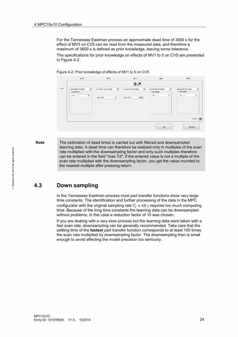
For the Tennessee Eastman process an approximate dead time of 3000 s for the effect of MV3 on CV5 can be read from the measured data, and therefore a maximum of 3600 s is defined as prior knowledge, leaving some tolerance. The specifications for prior knowledge on effects of MV1 to 5 on CV5 are presented in Figure 4-2. Figure 4-2: Prior knowledge of effects of MV1 to 5 on CV5

Note The estimation of dead times is carried out with filtered and downsampled learning data. A dead time can therefore be realized only in multiples of the scan rate multiplied with the downsampling factor and only such multiples therefore can be entered in the field "max Td". If the entered value is not a multiple of the scan rate multiplied with the downsampling factor, you get the value rounded to the nearest multiple after pressing return.

4.3 Down sampling In the Tennessee Eastman process most part transfer functions show very large time constants. The identification and further processing of the data in the MPC configurator with the original sampling rate 𝑇𝑠 = 60 𝑠 requires too much computing time. Because of the long time constants the learning data can be downsampled without problems, in this case a reduction factor of 10 was chosen. If you are dealing with a very slow process but the learning data were taken with a fast scan rate, downsampling can be generally recommended. Take care that the settling time of the fastest part transfer function corresponds to at least 100 times the scan rate multiplied by downsampling factor. The downsampling then is small enough to avoid affecting the model precision too seriously.


MPC10x10 Entry-ID: 101978659, V1.0, 10/2014 25

S

iem

ens

AG 2

014

All r

ight

s re

serv

ed

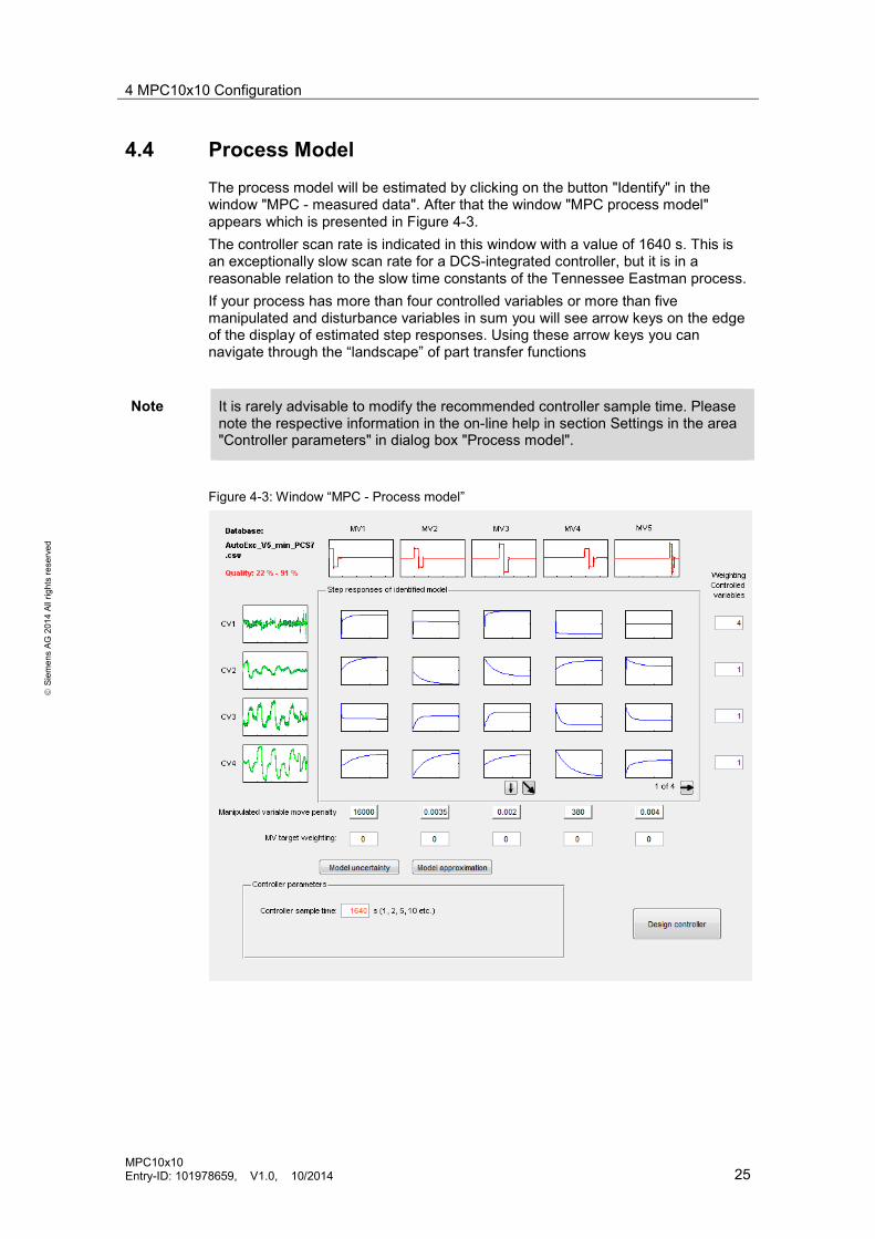
4.4 Process Model The process model will be estimated by clicking on the button "Identify" in the window "MPC - measured data". After that the window "MPC process model" appears which is presented in Figure 4-3. The controller scan rate is indicated in this window with a value of 1640 s. This is an exceptionally slow scan rate for a DCS-integrated controller, but it is in a reasonable relation to the slow time constants of the Tennessee Eastman process. If your process has more than four controlled variables or more than five manipulated and disturbance variables in sum you will see arrow keys on the edge of the display of estimated step responses. Using these arrow keys you can navigate through the “landscape” of part transfer functions

Note It is rarely advisable to modify the recommended controller sample time. Please note the respective information in the on-line help in section Settings in the area "Controller parameters" in dialog box "Process model".

Figure 4-3: Window “MPC - Process model”


MPC10x10 Entry-ID: 101978659, V1.0, 10/2014 26

S

iem

ens

AG 2

014

All r

ight

s re

serv

ed

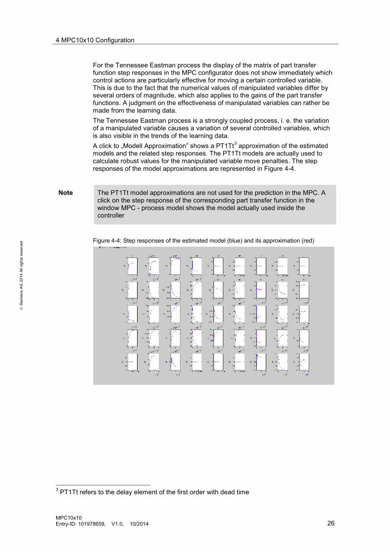
For the Tennessee Eastman process the display of the matrix of part transfer function step responses in the MPC configurator does not show immediately which control actions are particularly effective for moving a certain controlled variable. This is due to the fact that the numerical values of manipulated variables differ by several orders of magnitude, which also applies to the gains of the part transfer functions. A judgment on the effectiveness of manipulated variables can rather be made from the learning data. The Tennessee Eastman process is a strongly coupled process, i. e. the variation of a manipulated variable causes a variation of several controlled variables, which is also visible in the trends of the learning data. A click to „Modell Approximation” shows a PT1Tt3 approximation of the estimated models and the related step responses. The PT1Tt models are actually used to calculate robust values for the manipulated variable move penalties. The step responses of the model approximations are represented in Figure 4-4.

Note The PT1Tt model approximations are not used for the prediction in the MPC. A click on the step response of the corresponding part transfer function in the window MPC - process model shows the model actually used inside the controller

Figure 4-4: Step responses of the estimated model (blue) and its approximation (red)

3 PT1Tt refers to the delay element of the first order with dead time


MPC10x10 Entry-ID: 101978659, V1.0, 10/2014 27

S

iem

ens

AG 2

014

All r

ight

s re

serv

ed

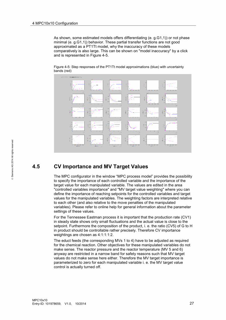
As shown, some estimated models offers differentiating (e. g.G1,1)) or not phase minimal (e. g.G1,1)) behavior. These partial transfer functions are not good approximated as a PT1Tt model, why the inaccuracy of these models comparatively is also large. This can be shown on "model inaccuracy" by a click and is represented in Figure 4-5. Figure 4-5: Step responses of the PT1Tt model approximations (blue) with uncertainty bands (red)

4.5 CV Importance and MV Target Values

The MPC configurator in the window “MPC process model” provides the possibility to specify the importance of each controlled variable and the importance of the target value for each manipulated variable. The values are edited in the area "controlled variables importance" and "MV target value weighting" where you can define the importance of reaching setpoints for the controlled variables and target values for the manipulated variables. The weighting factors are interpreted relative to each other (and also relative to the move penalties of the manipulated variables). Please refer to online help for general information about the parameter settings of these values. For the Tennessee Eastman process it is important that the production rate (CV1) in steady state shows only small fluctuations and the actual value is close to the setpoint. Furthermore the composition of the product, i. e. the ratio (CV5) of G to H in product should be controllable rather precisely. Therefore CV importance weightings are chosen as 4:1:1:1:2. The educt feeds (the corresponding MVs 1 to 4) have to be adjusted as required for the chemical reaction. Other objectives for these manipulated variables do not make sense. The reactor pressure and the reactor temperature (MV 5 and 6) anyway are restricted in a narrow band for safety reasons such that MV target values do not make sense here either. Therefore the MV target importance is parameterized to zero for each manipulated variable i. e. the MV target value control is actually turned off.


MPC10x10 Entry-ID: 101978659, V1.0, 10/2014 28

S

iem

ens

AG 2

014

All r

ight

s re

serv

ed

A comparatively high importance of MV target values can be useful if there are several manipulated variables which have similar effects but cause differently high costs. In this case please choose rather high target value importance for manipulated variables associated with high costs and specify after clicking on "design controller" in view “simulation parameters > MV target values” an economical favorable but still reachable value for these manipulated variables. Simulate the closed loop control system with different values of importance weightings to assess the consequences of the choice, see chapter 4.8 and online help. Choose high MV target value importance in comparison with the importance of certain controlled variables if reaching this manipulated variable target is so important that you accept a control error for these controlled variables.

Note MV targets are typically applied in combination with CV dead zones. It is recommended to specify MV target importance factors smaller than 0.01, such that MV targets will really become relevant only if all CVs are inside their zones. Note: if using set point prefilters in MPC10x10 function block, you have to specify even smaller values for MV target importance. Rather choose MV move penalties such that you do not need any prefilters to make sure that the relative importance of MV targets and CVs remains unspoiled.


MPC10x10 Entry-ID: 101978659, V1.0, 10/2014 29

S

iem

ens

AG 2

014

All r

ight

s re

serv

ed

4.6 Parameterization of MV Move Penalties You can specify the move penalty of the manipulated variables in the window “MPC - process model”. A large move for a certain manipulated variable in the MPC performance index means that this manipulated variable will be moved more slowly. A click on the input field “move penalty” of a manipulated variable opens a window like Figure 4-6 showing calculated values for optimal control performance and robust performance and the values chosen currently. The values for optimal performance deliver maximal control accuracy assuming high model quality while the values for robust performance assume a worst case scenario with respect to model precision. Figure 4-6: Window for parameterization of move penalties

The values for optimal performance are based on the PT1Tt model approximations, these for robust performance on an approximation of the error of these PT1Tt models. Since in the Tennessee Eastman process some part transfer functions do not show trends similar to 1st order lags, a calculation of the MV move penalties based on this assumption is very defensive, i. e. the move penalties will become high and the controller would behave accordingly slow.


MPC10x10 Entry-ID: 101978659, V1.0, 10/2014 30

S

iem

ens

AG 2

014

All r

ight

s re

serv

ed

Note In general it is recommended to choose the robust MV move penalties. If however at least on part transfer function identified by the MPC configurator is not similar to a first order lag, an adjustment of the MV move penalty for the corresponding manipulated variable is perhaps required. At first you run a simulation of the closed loop control system with the suggested values for robust performance and, if necessary, reduce the penalty values iteratively if the movement of the manipulated variables seem too hesitant to you.

The simulation in the MPC configurator uses a linearized process model. The behavior of most process plants is actually more or less nonlinear. Before you take the controller into PCS 7 and operate the real process, you should therefore select rather large MV move penalties with regard to model inaccuracies at first. Reduce the move penalties iteratively if the variation of the manipulated variables seem too hesitant to you. It is useful to store several sessions of the MPC configurator with different values for the move penalties in order to recall these different controller tunings quickly because the MV move penalties cannot be tuned at the PCS 7 function block.

4.7 Verifikation After clicking on the button “controller design" the window "MPC -verification and simulation” appears. Using the verification function you can check the quality of the model for the individual controlled variables. Click the button "load data”, select a file with verification data and choose the controlled, manipulated and disturbance variables in the same way as for the identification. After the click a window like (Figure 4-7) appears in which the trends of the original measured data and the controlled variables calculated by the model are shown. The deviation in [%] is calculated and displayed for each controlled variable. For the Tennessee Eastman process it turns out that the controlled variables CV3 and CV4, i. e. the concentration of E feed into the reactor and the concentration of B in purge are modelled less exactly. The reason might be that during recording of verification data in closed loop the manipulated variable amplitudes are much larger than in the learning data recorded in open loop. Since the Tennessee Eastman process shows a strongly nonlinear behavior, the estimated linear process model is no longer exactly valid for such large manipulated variable amplitudes.

Note Please take care that the verification data have the same structure as the identification data. Use the same sample time and make sure that the controlled, manipulated and disturbance variables (and even variables not used) are marked by the same variable names in the file.


MPC10x10 Entry-ID: 101978659, V1.0, 10/2014 31

S

iem

ens

AG 2

014

All r

ight

s re

serv

ed

Figure 4-7: Measured data (green) and simulated (using estimated process model) controlled variables (black). Recording of verification data was carried out in closed loop, unlike the learning data for process identification.

The function for verification of process model is particularly helpful if you are not satisfied with control performance of model predictive controller and suspect that this is due to a lack of model quality. In this case use the measured data from the closed loop control system as verification data and try to recognize those controlled variables that are not fitted properly by the model. You can try with several verification data sets in which different manipulated variables move more strongly or more weakly to find out which partial transfer functions are responsible for the low model quality. Now you can try to load additional learning data in which the effect of these part transfer functions is visible better, or you can describe these effects by physical considerations and enter parts of the process model as prior knowledge.

4.8 Simulation

4.8.1 Parameterization of Simulation

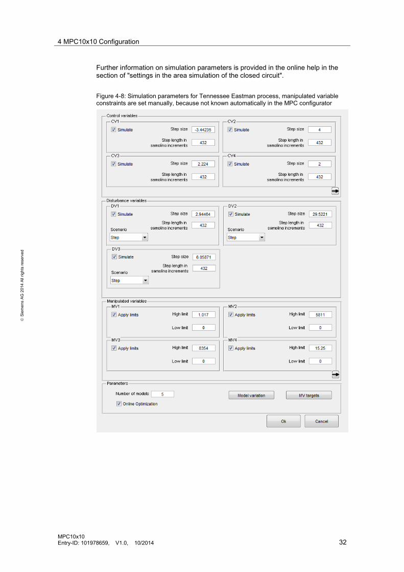
The button “simulate control system" in the window "MPC verification and simulation" is provided to simulate the behavior of the controller in combination with the plant for a certain configuration. It is recommended to simulate the closed control loop before you export the controller data to PCS 7. Although the simulation takes a certain computing time, costs and risks of a simulation are much lower than for experiments at the real plant You access the simulation settings by clicking the button "simulation parameters", opening a window like in Figure 4-8. For the MPC10x10 the values of step size and step duration respectively the high and low limits of the manipulated variables are displayed for up to four controlled, manipulated and disturbance variables at a time. To access further process values, click on the arrow keys at the lower right end of the appropriate fields of the user interface.


MPC10x10 Entry-ID: 101978659, V1.0, 10/2014 32

S

iem

ens

AG 2

014

All r

ight

s re

serv

ed

Further information on simulation parameters is provided in the online help in the section of "settings in the area simulation of the closed circuit". Figure 4-8: Simulation parameters for Tennessee Eastman process, manipulated variable constraints are set manually, because not known automatically in the MPC configurator


MPC10x10 Entry-ID: 101978659, V1.0, 10/2014 33

S

iem

ens

AG 2

014

All r

ight

s re

serv

ed

4.8.2 Model Variations and Simulation Results

Generally, it cannot be expected that the identified process model exactly fits to the behavior of the real plant, which makes the inclusion of model inaccuracies in the simulation a helpful feature. By the choice of the number of models in the window "simulation parameters" you can decide for how many different model variations the closed control loop is to be simulated (the first model is always the identified process model without variation). Because of computing time for large process models you can start simulating without model variations. As soon as you have found controller settings approximately corresponding to your ideas, you can carry out in-depth analysis with model variations. Random modifications of the models in the area defined by model inaccuracy are assumed if you do not specify them explicitly. If you want to simulate certain variations in certain part transfer functions, you find further information in the online help "settings in the area simulation of the closed circuit".

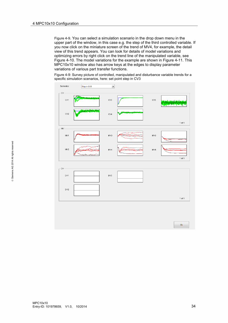
At the end of the simulation several windows with simulation results are shown, which however are rather difficult to read for large multivariable processes. Close these windows and click on the miniature display in the window "MPC - verification and simulation" to watch the detailed simulation results, see


MPC10x10 Entry-ID: 101978659, V1.0, 10/2014 34

S

iem

ens

AG 2

014

All r

ight

s re

serv

ed

Figure 4-9. You can select a simulation scenario in the drop down menu in the upper part of the window, in this case e.g. the step of the third controlled variable. If you now click on the miniature screen of the trend of MV4, for example, the detail view of this trend appears. You can look for details of model variations and optimizing errors by right click on the trend line of the manipulated variable, see Figure 4-10. The model variations for the example are shown in Figure 4-11. This MPC10x10 window also has arrow keys at the edges to display parameter variations of various part transfer functions. Figure 4-9: Survey picture of controlled, manipulated and disturbance variable trends for a specific simulation scenarios, here: set point step in CV3

http://dict.leo.org/ende/index_de.html#/search=scenario&searchLoc=0&resultOrder=basic&multiwordShowSingle=on


MPC10x10 Entry-ID: 101978659, V1.0, 10/2014 35

S

iem

ens

AG 2

014

All r

ight

s re

serv

ed

Figure 4-10: Simulated values for MV4, dark red: nominal model, red: model variations

Figure 4-11: Model variations of part transfer functions, in each case Kp: gain, Td: Dead time and Tp: time constant. The nominal values are represented by the green line, the yellow bar shows the model variation as deviations from nominal value in the range of model accuracy estimated from learning data.


MPC10x10 Entry-ID: 101978659, V1.0, 10/2014 36

S

iem

ens

AG 2

014

All r

ight

s re

serv

ed

4.8.3 Dynamic Online Optimization

The new MPC10x10 function block features dynamic online optimization: in contrary to ModPreCon, the MPC optimization problem (minimization of the specified performance index containing future control deviations, future manipulated variable moves and future deviations of manipulated variables from their target values) is solved in each sampling step considering constraints of active manipulated variable limits. Using the input parameter DynOptOn in CFC you can switch on/off the optimization for test purposes or for the saving computer power. If the online optimization is turned off the manipulated variable constrains are still respected correctly, but the ideal solution without considering constraints is just "cut off" (i. e. limited afterwards). This way you can obtain solutions that are only sub-optimal with respect to the original optimization problem inclusive constraints. If one or more manipulated variable constraints become active during plant operation, a higher control performance can be achieved by dynamic online optimization. You can activate or deactivate the dynamic online optimization by setting the tick-mark "online optimization" at the lower edge of the window "simulation parameters" in the MPC configurator for each simulation run. Sometimes after the simulation in the MPC configurator the following error message will appear: "Could not calculate the online optimization at every point in time". In this case the optimization algorithm did not find a solution for the dynamic optimization problem at particular time points for numeric reasons. The "cut off" solution of the unconstraint problem is used for these points of time. If the transient response as a whole meets the requirements, such small "gaps" in the optimization calculation are completely uncritical. For the Tennessee Eastman problem this can be displayed in the scenario "step in CV5". A detailed view of MV5 in this scenario is represented in Figure 4-12. If an error occurs during online optimization because of a specific model variation the trends of the controlled respectively the manipulated variables are displayed in gray instead of green respectively red as usual. Figure 4-12: Trend of MV5 for step in SP5 simulations without error in online optimization are red, simulations with error are gray.


MPC10x10 Entry-ID: 101978659, V1.0, 10/2014 37

S

iem

ens

AG 2

014

All r

ight

s re

serv

ed

Right click on the grey trend line and selecting "Show optimization errors" opens the window shown in Figure 4-13. In this view, the periods of time with errors in the online optimization are marked by grey bars. Figure 4-13: Display of the periods of time where the optimization problem with constraints has not been solved

5 Commissioning of the MPC10x10 in SIMATIC PCS 7

MPC10x10 Entry-ID: 101978659, V1.0, 10/2014 38

S

iem

ens

AG 2

014

All r

ight

s re

serv

ed


5.1 Download of Configuration Data The configuration data of the designed predictive controller are stored as SCL source by clicking the button "Export SCL code" in the window "MPC verification and simulation". Add this SCL file as an external source to the folder "sources" of your S7 program. Then open the SCL code, translate and download. Choose the value "True" at the binary input variable "Restart" of the MPC block in CFC to initialize the controller with the new configuration data.

Note You find detailed step by step instructions for download of configuration data in PCS 7 in the on-line help "Commissioning the controller in SIMATIC PCS 7”.

5.2 Limits Checking Check the controlled and manipulated variable parameters after compilation and download of source data of the predictive controller. The parameter values either result from linking or are specified at the inputs of the MPC10 x10 function block in CFC. At first open the faceplate of the MPC10x10 function block and select "CV parameters", opening a faceplate view like in Figure 5-1. Check whether the values specified in the columns "H range" and "L range" are corrected. The columns "H range optimization" and "L range optimization" are parameter settings for the economic operating point optimization which is not treated in the context of this application note. An operating point optimization would nevertheless be interesting for the Tennessee Eastman process because relevant business data are given in (Downs, 1993). The column "Dead band" defines in which zone small control deviations are ignored by the controller. You can specify the time constant of a setpoint prefilter to slow down the dynamic response for certain controlled variables. Neither dead bands nor prefilters are used in this example. Figure 5-1: CV parameters: High- and Low limits, dead bands and prefilters


MPC10x10 Entry-ID: 101978659, V1.0, 10/2014 39

S

iem

ens

AG 2

014

All r

ight

s re

serv

ed

Clicking the button "MV parameters" opens a view like in Figure 5-2. The limits of the manipulated variables for automatic mode are displayed. In addition, you have the possibility to specify gradient limits i. e. you can limit how far a manipulated variable may moves per sample step. Please note that the gradient limits are parameterized in MV units per second. In case of the slow Tennessee Eastman process the controller sample time is large and therefore the parameterized numerical values per second are small. The default precision of the gradient limits is two digits after the decimal point. This precision is linked to the precision of the manipulated variables by default. If you want to display more digits like in this example, you proceed as follows: At first open "Graphics Designer" in "WinCCExplorer". Click the button "Open" and select the OS picture in which the MPC10x10 block icon is located. Mark this block icon and select "Configurations" in view "Properties" of window “Object properties”. You will find the attributes "AnalogValueFormat" numbered from 1 to 24 here. The formats 1 to 10 determine the number of digits for CVs, the formats 11 to 20 for MVs and the formats 21 to 24 for DVs. Modify these formats as desired. Save the PDL file, open another picture in the OS and go back in order to make the modification visible. If you want to be very cautious you can set manipulated variable limits temporarily in a narrow band around the actual MV value before the controller is switched from manual to automatic mode for the first time. Figure 5-2: Manipulated variable parameters: High and Low limit, gradient limit. The unit ft³/h is used instead of kscmh for MV1 and MV4, because the unit kscmh is not available in PCS 7.


MPC10x10 Entry-ID: 101978659, V1.0, 10/2014 40

S

iem

ens

AG 2

014

All r

ight

s re

serv

ed

5.3 Commissioning Before you switch control mode from “manual” to “automatic” at the real process, check the controlled variable predictions for plausibility. In the MPC faceplate the predicted free response of the controlled variables for five representative points in the prediction horizon is displayed as vertical bars right to the bar of the actual CV values. These predicted values must start at the current CV values and, for constant manipulated variables they should reach a steady state which corresponds to the value that the actually measured controlled variables reach after sometime, see Figure 5-3. You can open the manipulated variable view represented in Figure 5-4 by clicking on the arrow at the lower edge of the standard view. Here you can check whether the manipulated variable limits for manual mode are definedcorrectly. If this should not be the case, check the parameters in the CFC of the controller block. Figure 5-3: MPC10x10 Standard view of the Tennessee Eastman process in manual operation mode. After the settling time the prediction bars (turquois), setpoint bars (blue) and controlled variable bars (green) are at the same height (if the manipulated variables are constant)


MPC10x10 Entry-ID: 101978659, V1.0, 10/2014 41

S

iem

ens

AG 2

014

All r

ight

s re

serv

ed

Figure 5-4: Manipulated variables screen in manual mode. The bar limits correspond to the MV limits for manual mode while the MV limits for automatic mode are indicated as small orange triangles. (In this case they are the same.)

If the MPC10x10 block is used as master controller in a cascade structure and the cascade logic works correctly, the following procedure is recommended for commissioning: • After the checking the prediction of the free response, make sure that the slave

controllers are still in automatic mode with internal setpoint. • Switch the MPC in automatic mode in the standard view. Now the MPC

manipulated variables are tracking the values from the slave controllers. • Switch the slave controllers to automatic with external setpoint. Now the MPC

will switch automatically from tracking mode to control mode. Check if this transition is carried out without bump.

• Wait until the MPC is in a steady state in automatic mode before you start active experiments for checking control performance, e. g. setpoint steps.

Note Further information on the connections of controllers in a cascade structure and correct tracking is provided in the application note "Configuration of Cascade Control" \5\.


MPC10x10 Entry-ID: 101978659, V1.0, 10/2014 42

S

iem

ens

AG 2

014

All r

ight

s re

serv

ed

It is recommended to record all relevant setpoints and actual values as well as manipulated variables of the MPC as archive variables. The trend display of the MPC faceplate can be switched to archive variables, such that longer time periods can be visualized without waiting after opening the trend view until enough new data are recorded. Check the cycle load of the SIMATIC CPU after activation of the MPC automatic mode to be on the safe side.

5.4 Controller Test Now the control performance of the designed predictive controller has to be checked. The controller is connected to the rigorous simulation of the Tennessee Eastman process which describes the nonlinear plant behavior as exactly as possible, unlike the linearized simulation inside the MPC configurator. This section is therefore equivalent to the test in a real plant.

The simulation time always is 72 ℎ, and setpoint steps or the activation of a disturbance take place after 2 ℎ. The simulation time in the following diagrams corresponds to the real process time while the simulation in PCS 7 runs twice as fast as real time.

5.4.1 Setpoint Steps

Production Rate Figure 5-5 shows the trend of the controlled and manipulated variables of the MPC for a setpoint step in CV1 that is a production rate reduction of −15%. This scenario is defined in the requirements in section 1.4. The diagram shows that the MPC is able to control the production rate fairly well although the concentration of B in purge (CV4) and the concentrations of A and E in reactor feed (CV2 and CV3) temporarily show small deviations from the setpoint.

Edcut A in Reactor Feed The step high to SP2, that is the concentration of A in reactor feed, is +4%, ending at 36,2%. This step leads to temporary, small deviations in CV 3 and 4 that is B in purge gas and E in reactor feed. The overall control performance is high as shown in Figure 5-6.

Edcut E in Reactor Feed The setpoint of CV3 that is the concentration of E in reactor feed is increased by 2.3 % in this scenario. To get a constant composition of the product (as indicated by CV5) anyway, the excessive educt E must react to by-product F. An increased feed of educt A is required. Figure 5-7 clearly shows that the predictive controller masters this task successfully. The concentration of G in product (CV5) remains constant and only temporary, minimal deviations from the setpoint of purge gas, that is CV4, can be recorded.


MPC10x10 Entry-ID: 101978659, V1.0, 10/2014 43

S

iem

ens

AG 2

014

All r

ight

s re

serv

ed

Inert Gas B in Purge This step of setpoint 4 is also a basic requirement from section 1.4. The concentration of inert gases B in the outlet has to be increased from 13.8 𝑚𝑜𝑙% to 15.8 𝑚𝑜𝑙%. This step can be managed very well by the MPC as shown in Figure 5-8. The other controlled variables remain constant and CV4 shows only a small overshoot.

Concentration of G in Product The step of setpoint 5 changes the ratio of component G to H in the product. Here the ratio is reduced from 50 𝑚𝑜𝑙% to 40 𝑚𝑜𝑙%, which corresponds to change required in section 1.4. Figure 5-9 shows the behavior of the MPC in this scenario. Similar to the step at SP1 it turns out that the predictive controller cannot decouple the controlled variables completely during the transient response: CV2, CV3 and CV4 temporarily show small deviations from the setpoints. The online optimization becomes active since the manipulated variables MV5 and MV6 touch the limits. Thanks to the optimization the MPC reaches a high control performance.


MPC10x10 Entry-ID: 101978659, V1.0, 10/2014 44

S

iem

ens

AG 2

014

All r

ight

s re

serv

ed

Figure 5-5: Step in production rate (SP1)

117

118

119

120

121

0 6 12 18 24 30 36 42 48 54 60 66 72

MV6

in [°

C]

T in [h]

MV6

2620

2640

2660

2680

2700

2720

0 6 12 18 24 30 36 42 48 54 60 66 72

MV5

in [k

Pa]

T in [h]

MV5

0

10

20

30

40

50

60

0 3 6 9 12 15 18 21 24 27 30 33 36 39 42 45 48 51 54 57 60 63 66 69 72T in [h]

SP1

SP2

SP3

SP4

SP5

CV1

CV2

CV3

CV4

CV5

00,05

0,10,15

0,20,25

0,3

0 6 12 18 24 30 36 42 48 54 60 66 72

MV1

in [k

scm

h]

T in [h]

MV1

2600280030003200340036003800

0 6 12 18 24 30 36 42 48 54 60 66 72

MV2

in [k

g/h]

T in [h]

MV2

7

7,5

8

8,5

9

9,5

0 6 12 18 24 30 36 42 48 54 60 66 72

MV4

in [k

scm

h]

T in [h]

MV4

32003400360038004000420044004600

0 6 12 18 24 30 36 42 48 54 60 66 72

MV3

in [k

g/h]

T in [h]

MV3


MPC10x10 Entry-ID: 101978659, V1.0, 10/2014 45

S

iem

ens

AG 2

014

All r

ight

s re

serv

ed

Figure 5-6: Step in concentration of A in reactor feed (SP2)

119,2119,4119,6119,8

120120,2120,4120,6

0 6 12 18 24 30 36 42 48 54 60 66 72

MV6

in [°

C]

T in [h]

MV6

2600262026402660268027002720

0 6 12 18 24 30 36 42 48 54 60 66 72

MV5

in [k

Pa]

T in [h]

MV5

0

10

20

30

40

50

60

0 3 6 9 12 15 18 21 24 27 30 33 36 39 42 45 48 51 54 57 60 63 66 69 72T in [h]

SP1

SP2

SP3

SP4

SP5

CV1

CV2

CV3

CV4

CV5

0

0,1

0,2

0,3

0,4

0 6 12 18 24 30 36 42 48 54 60 66 72

MV1

in [k

scm

h]

T in [h]

MV1

3600362036403660368037003720

0 6 12 18 24 30 36 42 48 54 60 66 72

MV2

in [k

g/h]

T in [h]

MV2

9,2

9,25

9,3

9,35

9,4

0 6 12 18 24 30 36 42 48 54 60 66 72

MV4

in [k

scm

h]

T in [h]

MV4

4400

4450

4500

4550

0 6 12 18 24 30 36 42 48 54 60 66 72

MV3

in [k

g/h]

T in [h]

MV3


MPC10x10 Entry-ID: 101978659, V1.0, 10/2014 46

S

iem

ens

AG 2

014

All r

ight

s re

serv

ed

Figure 5-7: Step in concentration of E in reactor feed (SP3)

119,6

119,8

120

120,2

120,4

120,6

0 6 12 18 24 30 36 42 48 54 60 66 72

MV6

in [°

C]

T in [h]

MV6

25802600262026402660268027002720

0 6 12 18 24 30 36 42 48 54 60 66 72

MV5

in [k

Pa]

T in [h]

MV5

0

10

20

30

40

50

60

0 3 6 9 12 15 18 21 24 27 30 33 36 39 42 45 48 51 54 57 60 63 66 69 72T in [h]

SP1

SP2

SP3

SP4

SP5

CV1

CV2

CV3

CV4

CV5

0,23

0,24

0,25

0,26

0,27

0,28

0 6 12 18 24 30 36 42 48 54 60 66 72

MV1

in [k

scm

h]

T in [h]

MV1

3640

3660

3680

3700

3720

0 6 12 18 24 30 36 42 48 54 60 66 72

MV2

in [k

g/h]

T in [h]

MV2

9,2

9,25

9,3

9,35

9,4

0 6 12 18 24 30 36 42 48 54 60 66 72

MV4

in [k

scm

h]

T in [h]

MV4

4450

4500

4550

4600

0 6 12 18 24 30 36 42 48 54 60 66 72

MV3

in [k

g/h]

T in [h]

MV3


MPC10x10 Entry-ID: 101978659, V1.0, 10/2014 47

S

iem

ens

AG 2

014

All r

ight

s re

serv

ed

Figure 5-8: Step in concentration of inert gas B in purge (SP4)

120,2

120,3

120,4

120,5

120,6

120,7

0 6 12 18 24 30 36 42 48 54 60 66 72

MV6

in [°

C]

T in [h]

MV6

2680

2700

2720

2740

2760

0 6 12 18 24 30 36 42 48 54 60 66 72

MV5

in [k

Pa]

T in [h]

MV5

0

10

20

30

40

50

60

0 3 6 9 12 15 18 21 24 27 30 33 36 39 42 45 48 51 54 57 60 63 66 69 72T in [h]

SP1

SP2

SP3

SP4

SP5

CV1

CV2

CV3

CV4

CV5

0,24

0,245

0,25

0,255

0,26

0,265

0 6 12 18 24 30 36 42 48 54 60 66 72

MV1

in [k

scm

h]

T in [h]

MV1

3620

3640

3660

3680

3700

0 6 12 18 24 30 36 42 48 54 60 66 72

MV2

in [k

g/h]

T in [h]

MV2

9,2

9,25

9,3

9,35

9,4

0 6 12 18 24 30 36 42 48 54 60 66 72

MV4

in [k

scm

h]

T in [h]

MV4

4400

4450

4500

4550

0 6 12 18 24 30 36 42 48 54 60 66 72

MV3

in [k

g/h]

T in [h]

MV3


MPC10x10 Entry-ID: 101978659, V1.0, 10/2014 48

S

iem

ens

AG 2

014

All r

ight

s re

serv

ed

Figure 5-9: Step in concentration of G in product (SP5)

118

120

122

124

126

0 6 12 18 24 30 36 42 48 54 60 66 72

MV6

in [°

C]

T in[h]

MV6

2700

2750

2800

2850

2900

0 6 12 18 24 30 36 42 48 54 60 66 72

MV5

in [k

Pa]

T in [h]

MV5

0

10

20

30

40

50

60

0 3 6 9 12 15 18 21 24 27 30 33 36 39 42 45 48 51 54 57 60 63 66 69 72T in [h]

SP1

SP2

SP3

SP4

SP5

CV1

CV2

CV3

CV4

CV5

0,22

0,23

0,24

0,25

0,26

0,27

0 6 12 18 24 30 36 42 48 54 60 66 72

MV1

in [k

scm

h]

T in [h]

MV1

0

1000

2000

3000

4000

0 6 12 18 24 30 36 42 48 54 60 66 72

MV2

in [k

g/h]

T in [h]

MV2

8,88,9

99,19,29,39,4

0 6 12 18 24 30 36 42 48 54 60 66 72

MV4

in [k

scm

h]

T in [h]

MV4

4000

4500

5000

5500

6000

0 6 12 18 24 30 36 42 48 54 60 66 72

MV3

in [k

g/h]

T in [h]

MV3


MPC10x10 Entry-ID: 101978659, V1.0, 10/2014 49

S

iem

ens

AG 2

014

All r

ight

s re

serv

ed

5.4.2 Disturbance Scenarios

Simulation results will be shown for the disturbing scenarios from Table 1-1. As not all disturbing scenarios can be described only a subset is shown. The following disturbing scenarios are successfully compensated by the base automation already such that they do not have to be considered in context of MPC: • Step in temperature of feed 2 (IDV3) • Step in condenser cooling water temperature (IDV5) • Random variation of feed 2 temperature (IDV9) • Random variation of feed 4 temperature (IDV10)

Concentration of Component B in Feed 4 The composition of feed stream 4 is modified in disturbance scenario IDV2. The educts A and C mainly reach the plant inside this stream but in addition, the inert gas B is also contained. The ratio between A and C is kept constant, but the concentration of inert gas in relation to the others educts is changed. Figure 5-10 shows the behavior of the MPC. The control performance is very good: there are only small temporary deviations of CV 2, 3 and 4 despite of the disturbing influence.

Step in Reactor Cooling Water Temperature Cooling water temperature for reactor cooling suddenly changes its value in this disturbing scenario (IDV4). As shown in Figure 5-10 this disturbing scenario is also controlled by the MPC, although noticeable deviations from the setpoint arise in CV3 and particularly in CV4. These deviations are compensated to zero in steady state and the overall control performances satisfactory.

Random Variation of the Reactor Cooling Water Temperature As opposed to the previous scenarios, now the fluctuations of the reactor cooling water temperature do not occur stepwise but randomly and permanently (IDV11). The disturbance was activated after 2 ℎ and deactivated after 42 ℎ in this scenario. Naturally this scenario is more difficult to handle for the predictive controller than the previous ones. Since now the reactor cooling water temperature permanently fluctuates, one variation of the MPC manipulated variable is followed by the next, such that the manipulated variables are oscillating as shown in Figure 5-11. Nevertheless the MPC is able to keep the controlled variables stable in a zone around the setpoint, and when the disturbance ends after 42 ℎ the controlled and manipulated variables calm down again.

Drift of Reaction Kinetics Figure 5-12 shows the trend of the controlled and manipulated variables for a drift in reaction kinetics (IDV13). This disturbance was also activated after 2 ℎ and deactivated after 42 ℎ simulation time to be able to evaluate the behavior of the predictive controller after the end of the disturbance. Similar to the previous disturbance, the controlled and manipulated variables are oscillating, but this time with larger amplitude. However the oscillation is stable and longer simulation experiments which are not recorded here for clarity reasons confirm that the system remains stable. This scenario shows once more that the predictive controller is able to bring back the process to the original operating point after the drift is switched off.


MPC10x10 Entry-ID: 101978659, V1.0, 10/2014 50

S

iem

ens

AG 2

014

All r

ight

s re

serv

ed

Figure 5-10: Stepwise variation of reactor cooling water temperature (IDV4)

119

119,5

120

120,5

0 6 12 18 24 30 36 42 48 54 60 66 72

MV6

in [°

C]

T in [h]

MV6

2550

2600

2650

2700

2750

0 6 12 18 24 30 36 42 48 54 60 66 72

MV5

in [k

Pa]

T in [h]

MV5

0

10

20

30

40

50

60

0 3 6 9 12 15 18 21 24 27 30 33 36 39 42 45 48 51 54 57 60 63 66 69 72T in [h]

SP1

SP2

SP3

SP4

SP5

CV1

CV2

CV3

CV4

CV5

0,23

0,24

0,25

0,26

0,27

0 6 12 18 24 30 36 42 48 54 60 66 72

MV1

in [k

scm

h]

T in [h]

MV1

3620364036603680370037203740

0 6 12 18 24 30 36 42 48 54 60 66 72

MV2

in [k

g/h]

T in [h]

MV2

9,25

9,3

9,35

9,4

9,45

9,5

0 6 12 18 24 30 36 42 48 54 60 66 72

MV4

in [k

scm

h]

T in [h]

MV4

4350440044504500455046004650

0 6 12 18 24 30 36 42 48 54 60 66 72

MV3

in [k

g/h]

T in [h]

MV3


MPC10x10 Entry-ID: 101978659, V1.0, 10/2014 51

S

iem

ens

AG 2

014

All r

ight

s re

serv

ed

Figure 5-11: Random variation of reactor cooling water temperature (IDV11), activated at 2 h simulation time, deactivated after 42 h

118,5

119

119,5

120

120,5

121

0 6 12 18 24 30 36 42 48 54 60 66 72

MV6

in [°

C]

T in [h]

MV6

2550

2600

2650

2700

2750

2800

0 6 12 18 24 30 36 42 48 54 60 66 72

MV5

in [k

Pa]

T in [h]

MV5

0

10

20

30

40

50

60

0 3 6 9 12 15 18 21 24 27 30 33 36 39 42 45 48 51 54 57 60 63 66 69 72T in [h]

SP1

SP2

SP3

SP4

SP5

CV1

CV2

CV3

CV4

CV5

0,230,235

0,240,245

0,250,255

0,26

0 6 12 18 24 30 36 42 48 54 60 66 72

MV1

in [k

scm

h]

T in [h]

MV1

3500

3550

3600

3650

3700

3750

0 6 12 18 24 30 36 42 48 54 60 66 72

MV2

in [k

g/h]

T in [h]

MV2

9,1

9,2

9,3

9,4

9,5

0 6 12 18 24 30 36 42 48 54 60 66 72

MV4

in [k

scm

h]

T in [h]

MV4

4350440044504500455046004650

0 6 12 18 24 30 36 42 48 54 60 66 72

MV3

in [k

g/h]

T in [h]

MV3


MPC10x10 Entry-ID: 101978659, V1.0, 10/2014 52

S

iem

ens

AG 2

014

All r

ight

s re

serv

ed

Figure 5-12: Drift of the reaction kinetics (IDV13)

118

119

120

121

122

0 6 12 18 24 30 36 42 48 54 60 66 72

MV6

in [°

C]

T in [h]

MV6

2500255026002650270027502800

0 6 12 18 24 30 36 42 48 54 60 66 72

MV5

in [k

Pa]

T in [h]

MV5

0

10

20

30

40

50

60

0 3 6 9 12 15 18 21 24 27 30 33 36 39 42 45 48 51 54 57 60 63 66 69 72T in [h]

SP1

SP2

SP3

SP4

SP5

CV1

CV2

CV3

CV4

CV5

0,22

0,23

0,24

0,25

0,26

0,27

0 6 12 18 24 30 36 42 48 54 60 66 72

MV1

in [k

scm

h]

T in [h]

MV1

3500355036003650370037503800

0 6 12 18 24 30 36 42 48 54 60 66 72

MV2

in [k

g/h]

T in [h]

MV2

99,19,29,39,49,59,6

0 6 12 18 24 30 36 42 48 54 60 66 72

MV4

in [k

scm

h]

T in [h]

MV4

43004350440044504500455046004650

0 6 12 18 24 30 36 42 48 54 60 66 72

MV3

in [k

g/h]

T in [h]

MV3


MPC10x10 Entry-ID: 101978659, V1.0, 10/2014 53

S

iem

ens

AG 2

014

All r

ight

s re

serv

ed

5.4.3 Comparison of Simulation inside MPC Configurator to Real Process (Rigorous Simulation Model)

An example in this section will show how the simulation inside the MPC configurator can be different from the real process. In the MPC configurator, based on the nominal linear model random model variations (still linear models) are created to make the consequences of the model uncertainty visible. The real process is represented in PCS 7 by the simulation model from section 1.3 and contains all non-linear effects. In Figure 5-12, once again the trends of the manipulated variables and the controlled variable CV3 are shown in combination with the simulation data from the MPC configurator. (The trends of the other controlled variables are omitted for clarity since they follow the setpoints anyway.) From the figure you can see that MV2 to MV6 are located within the area defined by the trends of the random model variations of the MPC configurator. This means that these model variations are a reasonable representation of the range of possible behavior patterns of the real process. The setpoint step in the simulation of MPC configurator takes almost the same time as the real process, but you see that noise level of CV3 is greater than assumed by the MPC configurator. Probably the process is affected by un-modelled (not modelled in the MPC) disturbances which result in larger oscillation amplitudes.


MPC10x10 Entry-ID: 101978659, V1.0, 10/2014 54

S

iem

ens

AG 2

014

All r

ight

s re

serv

ed

Figure 5-13: Comparison between manipulated and controlled variables from MPC configurator (nominal model: dark gray, model variations: light gray) and control response of the process simulation in PCS 7colored: pink, green, blue, black)

0,230,240,250,260,270,28

0 6 12 18 24 30 36 42 48 54 60 66 72

MV1

in [k

scm

h]

T in [h]

MV1

3600

3650

3700

3750

0 6 12 18 24 30 36 42 48 54 60 66 72

MV2

in [k

g/h]

T in [h]

MV2

4350

4400

4450

4500

4550

4600

0 6 12 18 24 30 36 42 48 54 60 66 72

MV3

in [k

g/h]

T in [h]

MV3

9,15

9,2

9,25

9,3

9,35

9,4

0 6 12 18 24 30 36 42 48 54 60 66 72

MV4

in [k

scm

h]

T in [h]

MV4

2550

2600

2650

2700

2750

0 6 12 18 24 30 36 42 48 54 60 66 72

MV5

in [k

Pa]

T in [h]

MV5

119,2119,4119,6119,8

120120,2120,4120,6

0 6 12 18 24 30 36 42 48 54 60 66 72

MV6

in [°

C]

T in [h]

MV6

16

17

18

19

20

21

22

23

0 4 8 12 16 20 24 28 32 36 40 44 48 52 56 60 64 68 72

E in

Rea

ktor

zufu

hr in

[mol

%]

T in [h]

CV3

6 Benefit for Plant Operator Company

MPC10x10 Entry-ID: 101978659, V1.0, 10/2014 55

S

iem

ens

AG 2

014

All r

ight

s re

serv

ed

6 Benefit for Plant Operator Company The Tennessee Eastman benchmark process is well known in the worldwide control engineering community as a particularly ambitious control problem. The chemical process is carried out in five plant units which are connected by material flows. Besides the strongly exothermic chemical reaction the recycling stream causes additional dynamic effects from the rear plant section (separator) back into the reactor. The process is dynamically unstable, strongly interacting and strongly nonlinear from the control engineering point of view. In addition, it shows dead times, non-minimal phase responses as well as extremely slow time constants. Nevertheless the MPC10x10 as a plant-wide master controller with 5 controlled variables, 6 manipulated variables and 3 measured disturbance variables together with a base automation including almost 20 carefully coordinated PID controllers is able to fulfill the requirements on the automation: • Keep reactor pressure, temperature and all levels inside constraints • Minimize the variability of product quality and production rate • Minimize valve movements • Compensate disturbances • Change production rate (setpoint step CV1) or product mix (setpoint step CV5)

during ongoing chemical reaction • Change reaction conditions (concentration of A or E in reactor feed) or

concentration of B in purge during ongoing reaction. The MPC10x10 function block for the first time allows solving such ambitious MPC applications with a DCS integrated multivariable controller. The performance of the MPC10x10 including online optimization comes close to PC based "full-blown" MPC software packages, but regarding availability, usability and cost efficiency, the MPC10x10 still offers the immanent advantages of DCS integrated control functions.

7 Related Literature

MPC10x10 Entry-ID: 101978659, V1.0, 10/2014 56

S

iem

ens

AG 2

014

All r

ight

s re

serv

ed

7 Related Literature Table 7-1

Topics Title

\1\ Siemens Industry Online Support


\2\ Download page of this application note


\3\ Tennessee Eastman Process model

Downs, J. J. (Vol. 17, No. 3, 1993). A plant-wide industrial process control problem. Computers & Chemical Engineering, S. 245-255.

\4\ Tennessee Eastman base Control and MPC

Ricker, N. (1995). Nonlinear Model Predictive Control of the Tennessee Eastman Challenge Process. Computers and Chemical Engineering, pp. 961-981.

\5\ Applikation note

Configurating of Cascade Control (Entry-ID: 43033319) http://support.automation.siemens.com/WW/view/en/43033319

8 History Tabelle 8-1

Version Date Revisions

V1.0 10/2014 First release




0 Appendix

MPC10x10 Entry-ID: 101978659, V1.0, 10/2014 57

S

iem

ens

AG 2

014

All r

ight

s re

serv

ed

Appendix Table A-1: Manipulated variables of Tennessee Eastman process simulation

Manipulated Variable Operating Point Variable Number

Feed valve D (Stream 2) 63.053 % XMV1

Feed valve E (Stream 3) 53.980 % XMV2

Feed valve A (Stream 1) 24.644 % XMV3

Feed valve A and C (Stream 4) 61.302 % XMV4

Compressor recycle valve 22.210 % XMV5

Purge valve 40.064 % XMV6

Separator outlet valve 38.100 % XMV7

Stripper outlet valve 46.534 % XMV8

Stripper steam valve 47.446 % XMV9 Reactor cooling water flow valve 41.106 % XMV10

Condenser cooling water flow valve 18.114 % XMV11

Agitator speed 200 U min� XMV12

Table A-2: Measured values from Tennessee Eastman Process simulation

Measured value Operating Point Variable Number

Feed A (Stream 1) 0.25052 kscmh XMEAS1

Feed D (Stream 2) 3664.0 kgh� XMEAS2

Feed E (Stream 3) 4509.3 kgh� XMEAS3

Feed A und C (Stream 4) 9.3477 kscmh XMEAS4

Recycle flow (Strom 8) 26.902 kscmh XMEAS5

Reactor feed rate (Stream 6)

42.339 kscmh XMEAS6

Reactor pressure 2705.0 kPa XMEAS7

Reactor level 75.000 % XMEAS8

Reactor temperature 120.4 °C XMEAS9

Purge rate 0.33712 kscmh XMEAS10

Product separator temperature

80.109 °C XMEAS11

Product separator level 50 % XMEAS12

Product separator pressure 2633.7 kPa XMEAS13

Product separator flow 25.160 m3

h� XMEAS14

Stripper level 50 % XMEAS15

Stripper pressure 3102.2 kPa XMEAS16

Stripper under flow (Stream 11)

22.949 m3

h� XMEAS17

Stripper temperature 65.731 °C XMEAS18

Stripper steam flow 230.31 kgh� XMEAS19

0 Appendix

MPC10x10 Entry-ID: 101978659, V1.0, 10/2014 58

S

iem

ens

AG 2

014

All r

ight

s re

serv

ed

Measured value Operating Point Variable Number

Compressor power 341.43 kW XMEAS20

Reactor cooling water outlet temperature

94.599 °C XMEAS21

Separator cooling water outlet temperature

77.297 °C XMEAS22

Table A-3: Component concentrations in Stream 6

Component Operating Point Variable Number

A 32.188 mol% XMEAS23

B 8.8933 mol% XMEAS24

C 26.383 mol% XMEAS25

D 6.8820 mol% XMEAS26

E 18.776 mol% XMEAS27

F 1.6567 mol% XMEAS28

These component concentrations are provided by an analyzer which has a sampling rate of 6𝑚𝑖𝑛 and dead time of 6𝑚𝑖𝑛. Table A-4: Component concentrations in Stream 9


A 32.958 mol% XMEAS29

B 13.823 mol% XMEAS30

C 23.978 mol% XMEAS31




G 4.8436 mol% XMEAS35

H 2.2986 mol% XMEAS36

These component concentrations are provided by an analyzer which has a sampling rate of 6𝑚𝑖𝑛 and dead time of 6𝑚𝑖𝑛. Table A-5: Component concentrations in Stream 11





G 53.724 mol% XMEAS40

H 43.828 mol% XMEAS41

These component concentrations are provided by an analyzer which has a sampling rate of 15 𝑚𝑖𝑛 and dead time of 15 𝑚𝑖𝑛.

Configuration of the MPC10x10 for Tennessee Eastman ...€¦ · thermodynamic and chemical...

Documents

Transcript of Configuration of the MPC10x10 for Tennessee Eastman ...€¦ · thermodynamic and chemical...