3. Confidence intervals

“Confidence is what you have before you understand the problem”

Woody Allen

2

Confidence intervalsn Sample mean, 𝑀, estimates the true mean, 𝜇n How good is 𝑀?

n Confidence interval: a range [𝑀𝐿, 𝑀𝑈], where we expect the true mean be with a certain confidence

n This can be done for any population parameter

o meano mediano standard deviationo correlationo proportiono etc.

Populationunknown mean 𝜇

unknown standard deviation 𝜎other parameters

Samplesize 𝑛

mean 𝑀st. dev. 𝑆𝐷

other statistics

Mea

sure

d va

lue

Sample mean, 𝑀

Confidence interval

3

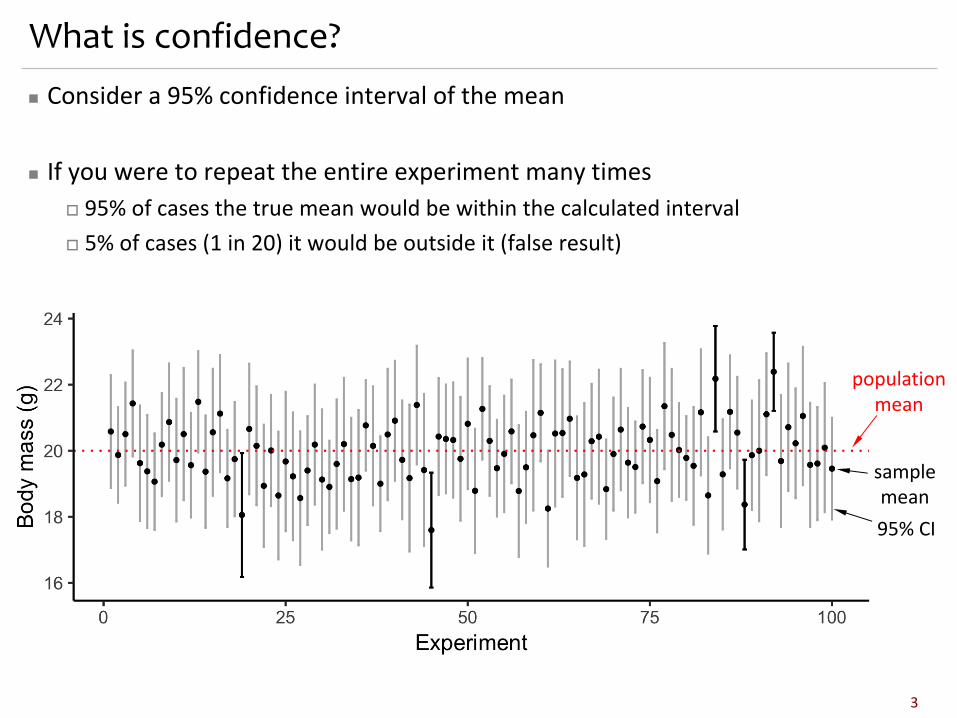
What is confidence?n Consider a 95% confidence interval of the mean

n If you were to repeat the entire experiment many timeso 95% of cases the true mean would be within the calculated intervalo 5% of cases (1 in 20) it would be outside it (false result)

samplemean95% CI

populationmean

Why 95%?n Textbook by Ronald Fisher (1925)n He thought 95% confidence interval was

“convenient” as it resulted in 1 false indication in 20 trials

n He published tables for a few probabilities, including 𝑝 = 5%

n The book had become one of the most influential textbooks in 20th century statistics

n However, there is nothing special about 95% confidence interval or p-value of 5%

4

Ronald Fishern Probably the most influential statistician

of the 20th centuryn Also evolutionary biologistsn Went to Harrow School and then

Cambridgen Arthur Vassal, Harrow’s schoolmaster:

I would divide all those I had taughtinto two groups: one containing asingle outstanding boy, Ronald Fisher;the other all the rest

n Didn’t like administration and admin people: “an administrator, not the highest form of human life”

5

Ronald Fisher (1890-1962)

Sampling distributionn Gedankenexperimentn Consider an unknown populationn Draw lots of samples of size 𝑛n Calculate an estimator from each

sample

n Build a frequency distribution of the estimator

n This is a sampling distribution

n Width of the sampling distribution is a standard error

6

Examples of sampling distribution

105 samples of 𝑛 = 5 from 𝒩(20, 5)

Confidence interval of the mean

Sampling distribution of the meann The distribution curve represents all

samplesn Keep the region corresponding to the

required confidence, e.g. 95%n Reject 2.5% on each siden This gives a confidence interval of the

mean

8

100,000 samples of 5 mice from normal population with 𝜇 = 20 g and 𝜎 = 5 g

Mean body weight calculated for each sample

Interval containing95% of samples

M (g)

Desired fraction95%

Reject 2.5%Reject 2.5%

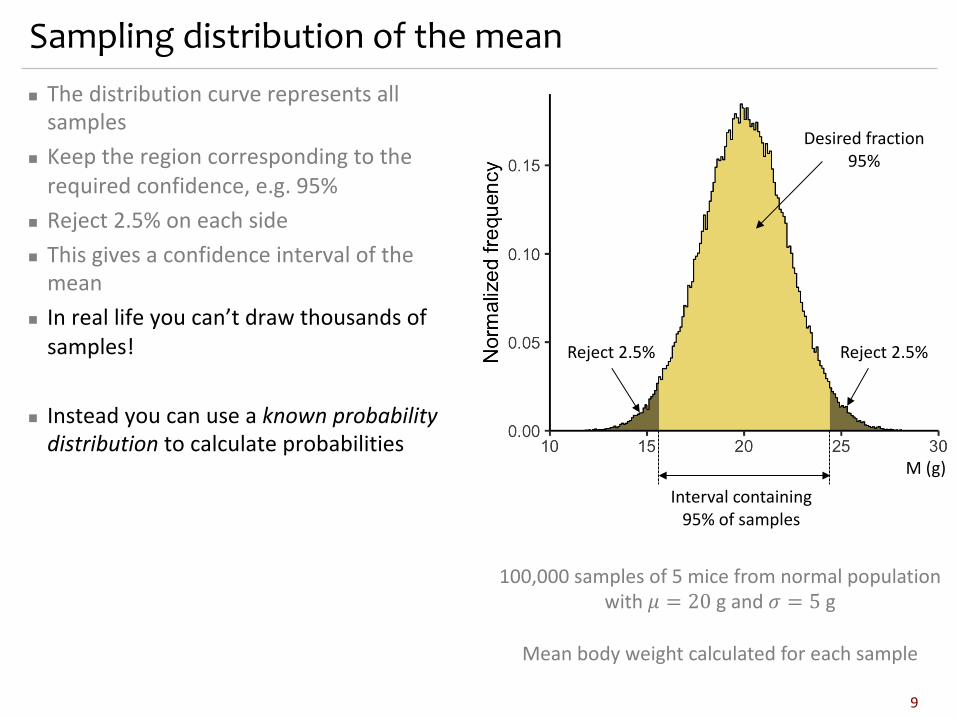
Sampling distribution of the meann The distribution curve represents all

samplesn Keep the region corresponding to the

required confidence, e.g. 95%n Reject 2.5% on each siden This gives a confidence interval of the

meann In real life you can’t draw thousands of

samples!

n Instead you can use a known probability distribution to calculate probabilities

9

100,000 samples of 5 mice from normal population with 𝜇 = 20 g and 𝜎 = 5 g

Mean body weight calculated for each sample

Interval containing95% of samples

M (g)

Desired fraction95%

Reject 2.5%Reject 2.5%

Sampling distribution of the meann For the given sample find 𝑀, 𝑆𝐷 and 𝑛 let

us define a statistic

𝑡 =𝑀 − 𝜇𝑆𝐸

n Mathematical trick – we cannot calculate 𝑡

n Gedankenexperiment: create a sampling distribution of 𝑡

10

100,000 samples of 5 mice from normal population with 𝜇 = 20 g and 𝜎 = 5 g

Mean body weight calculated for each sample

Interval containing95% of samples

M (g)

Desired fraction95%

Reject 2.5%Reject 2.5%

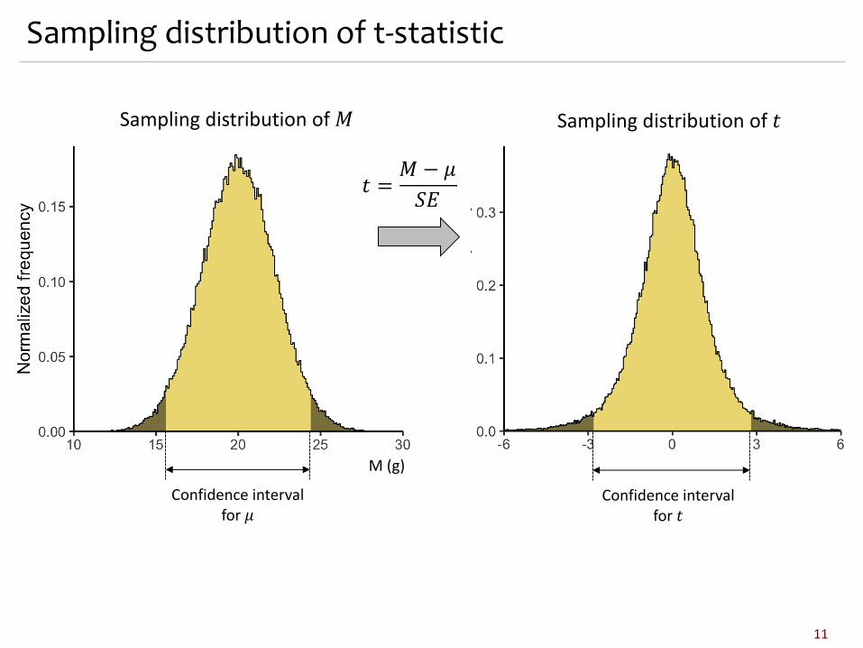
Sampling distribution of t-statistic

11

Confidence intervalfor 𝜇

M (g)

Confidence intervalfor 𝑡

𝑡 =𝑀 − 𝜇𝑆𝐸

Sampling distribution of 𝑀 Sampling distribution of 𝑡

12

Confidence interval of the meann Statistic

𝑡 =𝑀 − 𝜇𝑆𝐸

has a known sampling distribution: Student’s t-distribution with 𝑛 − 1degrees of freedom

n We can calculate probabilities!

Normal

William Gossetn Brewer and statisticiann Developed Student’s t-distribution

n Worked for Guinness, who prohibited employees from publishing any papers

n Published as “Student”

n Worked with Fisher and developed the t-statistic in its current form

n Always worked with experimental datan Progenitor bioinformatician?

13

William Sealy Gosset (1876-1937)

William Gossetn Brewer and statisticiann Developed Student’s t-distribution

n Worked for Guinness, who prohibited employees from publishing any papers

n Published as “Student”

n Worked with Fisher and developed the t-statistic in its current form

n Always worked with experimental datan Progenitor bioinformatician?

14

15

Confidence interval of the meann Statistic

𝑡 =𝑀 − 𝜇𝑆𝐸

has a known sampling distribution: Student’s t-distribution with 𝑛 − 1degrees of freedom

n We can find a critical value of 𝑡! to cut off required confidence interval

n R function qt

n Confidence interval on 𝑡 is [−𝑡! , +𝑡!]

95% confidence interval of 𝑡

Desired fraction95%

Reject 2.5%Reject 2.5%

Student’s t-distribution

𝑡!−𝑡!

16

Confidence interval of the meann We used transformation

𝑡 =𝑀 − 𝜇𝑆𝐸

n Confidence interval on t is [−𝑡! , +𝑡!]

n Find 𝜇 from the equation above

𝜇 = 𝑀 + 𝑡𝑆𝐸

n From limits on 𝑡 we find limits on 𝜇:

𝑀" = 𝑀 − 𝑡!𝑆𝐸𝑀# = 𝑀 + 𝑡!𝑆𝐸

n Or

𝜇 = 𝑀 ± 𝐶𝐼

where confidence interval is a scaled standard error

𝐶𝐼 = 𝑡!𝑆𝐸

95% confidence interval of 𝑡

Desired fraction95%

Reject 2.5%Reject 2.5%

Student’s t-distribution

𝑡!−𝑡!

How to use t-distribution to get 95% CI of the mean

17

Confidence intervalfor 𝜇

M (g)

Confidence intervalfor 𝑡

𝑡 =𝑀 − 𝜇𝑆𝐸

Sampling distribution of 𝑀Student’s 𝑡-distribution𝑛 − 1 degrees of freedom

𝑀" = 𝑀 − 𝑡!𝑆𝐸𝑀# = 𝑀 + 𝑡!𝑆𝐸

𝑀" 𝑀# 𝑡!−𝑡!

18

Exercise: 95% confidence interval for the meann We have 5 mice with measured body weights

16.8, 21.8, 29.2, 23.3 and 26.3 gn Estimators from the sample

𝑀 = 23.48 g𝑆𝐷 = 4.69 g𝑆𝐸 = 2.10 g

23.48 ± 5.83 g

𝑡! = 2.776

n Confidence limits are

𝑀" = 𝑀 − 𝑡!𝑆𝐸 = 17. 65 g𝑀# = 𝑀 + 𝑡!𝑆𝐸 = 29.31 g

n Estimate of the mean with 95% confidence is

𝜇 = 23 ± 6 g

n Critical value from t-distribution for two-tail probability and 4 degrees of freedom

Confidence intervalfor 𝑡

𝑡!−𝑡!

Confidence interval in R> d <- c(16.8, 21.8, 29.2, 23.3, 26.3)> n <- length(d)> M <- mean(d)> SE <- sd(d) / sqrt(n)# critical t> tc <- qt(0.975, df = n - 1)# lower confidence limit> M - tc * SE[1] 17.65118# upper confidence limit> M + tc * SE[1] 29.30882

19

0.95

0.025

p = 0.975

tc = qt(0.975, df = 4)[1] 2.776445

p = pt(tc)

tc = qt(p)

Confidence interval in R: the simple way> d <- c(16.8, 21.8, 29.2, 23.3, 26.3)> t.test(d)

One Sample t-test

data: dt = 11.184, df = 4, p-value = 0.0003639alternative hypothesis: true mean is not equal to 095 percent confidence interval:17.65118 29.30882sample estimates:mean of x

23.48

20

Confidence interval vs. standard error

21

Confidence interval

Interval containing 95% of samples

𝜎$ =𝜎𝑛

Width of thesampling distribution

Standard error

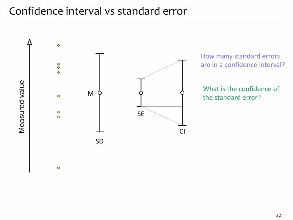
Confidence interval vs standard error

22

How many standard errors are in a confidence interval?

What is the confidence of the standard error?M

SD

SE

CI

Confidence interval vs standard error

23

1.96

Number of standard errors in a 95% CI

Confidence ofa standard error

0.68

Large samples:

95% 𝐶𝐼 ≈ 2 𝑆𝐸

Confidence of SE is ~68%

YOU NEEDmore

REPLICATES

25

SD, SE and 95% CI

n Normal population of 𝜇 = 20 g and 𝜎 = 5 gn Sample of 𝑛 = 8 and 𝑛 = 100

𝑛 = 8 𝑛 = 100

26

2 replicates? NO!

𝑛 = 2

Example: confidence intervalsn Experiment where a reporter measures

transcriptional activity of a geneo Day 1: 3 biological replicateso Day 2: 5 biological replicates

n Normalized data:

n 95% confidence intervals for the mean:Day 1: [0.87, 0.94]Day 2: [0.56, 0.84]

n What can you say about these results? What else can you do with these data?

27

Day 1 0.89 0.92 0.90Day 2 0.55 0.76 0.61 0.83 0.75

𝑝 = 0.03

Confidence interval of the median

Confidence interval of the mediann We do not build a sampling distributionn Draw one random sample of 𝑛 points, one by one: 𝑥!, 𝑥", … , 𝑥#n Population median 𝜃 property: 𝑃 𝑥$ < 𝜃 = !

"and 𝑃 𝑥$ > 𝜃 = !

"n For each data point we have fifty-fifty chance

29

14.9 15.6 18.6 19.1 20.1 20.6 21.4 24.8

𝑃 = 0.273

1. Let true median 𝜃 = 20

𝑃 = 0.031

2. Let true median 𝜃 = 15

Limited confidence intervals of the median

30

reject 2.5% reject 2.5%

99.2%14.9 15.6 18.6 19.1 20.1 20.6 21.4 24.8

93.0%

14.9 15.6 18.6 19.1 20.1 20.6 21.4 24.8

71.1%

14.9 15.6 18.6 19.1 20.1 20.6 21.4 24.8

Confidence interval of the median - interpolationn Approach based on all pairs of data points and interpolationn Hodges-Lehmann estimator

> x <- c(14.9, 15.6, 18.6, 19.1, 20.1, 20.6, 21.4, 24.8)> wilcox.test(x, conf.int = TRUE)

Wilcoxon signed rank test

data: xV = 36, p-value = 0.007813alternative hypothesis: true location is not equal to 095 percent confidence interval:16.75 22.45sample estimates:(pseudo)median

19.6

31

Replicates

Replicatesn Replication is the repetition of an experiment under the same conditionsn Typically, the only way of estimating measurement errors is to do the experiment

in replicates

n You need replicates, but how many?

n Statistical powern Roughly speaking, there are two cases

o to get an estimate with a required precisiono to get enough sensitivity for differential analysis

33

Number of replicates to find the meann Sampling distribution of the mean has 𝜎$ = 𝜎/ 𝑛

n Interval ~2𝜎$ around the true mean contains 95% of all samples

n Let’s call it precision of the mean:

𝜖 ≈ 2𝜎$ =2𝜎𝑛

34

Sampling distribution of the mean

𝜎! =𝜎𝑛

n Sample size to get the required precision:

𝑛 =4𝜎%

𝜖%

n This requires a priori knowledge of 𝜎(do a pilot experiment to estimate)

n Example: 𝜎 = 5 g, required precision of ±2 g

𝑛 = 4×5 g %

2 g % = 25

𝜎 = 5 g𝑛 = 30

Hand-outs available at https://dag.compbio.dundee.ac.uk/training/Statistics_lectures.html