CONFIDENCE INTERVALS ON µWHEN IS UNKNOWNσ

A. Introduction

1. this situation, where we do not know anything about the population but the sample characteristics, is far and away the most common circumstance

2. when we do not know (the standard deviation of the population), we again use the standard error of µ( ), but calculate it in a different fashion.

σ

µSE

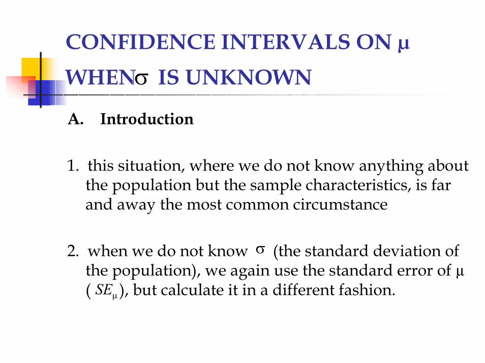
Introduction (cont’d)

3. an unbiased estimate

a. this formula is different from the one that Spatz (1997) uses

b. recall how using n-1 in the denominator of the variance helps us to determine an unbiased estimate for the population variance

==sSE xσµ 1−n

Introduction (cont’d)

4. since we do not know , we cannot use zand what we know about the normal curve to generate CI’s on µ

5. instead, we use the Student’s t distribution

a. the t-distribution is used with small samples (especially when n < 30) where the population variance is unknown

σ

Introduction (cont’d)

b. the t is a theoretical distribution like the normal, and, like the normal, it is a family of curves

c. it is unimodal, bell-shaped, and symmetrical like the normal

d. it was popularized by W.S. Gossett in 1908, who signed his original paper as “Student”

e. the larger the sample, the “more closely the t approximates the normal distribution. For samples larger than 120, they are

practically equivalent” (Vogt, 1999, p. 282).

Computation of confidence intervals on µ

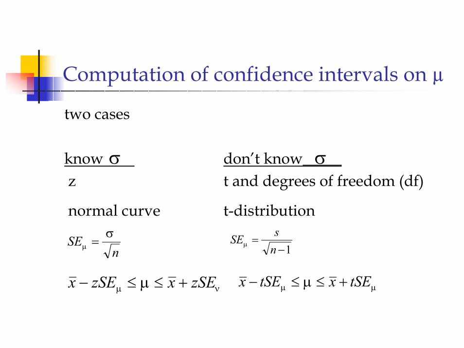
two cases

know don’t know_____ z t and degrees of freedom (df)

normal curve t-distribution

σ σ

nSE σ

µ = 1−=nsSEµ

νµ µ zSExzSEx +≤≤− µµ µ tSExtSEx +≤≤−

C. Shape of the t-distribution

Refer to Spatz (1997, p. 155, Figure 6.5)

1. as n, sample size, increases, the t-distribution approaches the normal

2. this relationship holds because, as n increases, df (degrees of freedom) increase

D. Table of the t-distribution

Refer to Spatz (1997, p. 371, Table D)

1. look first at the significance level for two-tailed test at the confidence level we want, e.g.,

=significance level = 1 – confidence levelα

Table of the t-distribution (cont’d)

2. first column in this table indicates degrees of freedom (df)

a. generally speaking, degrees of freedom tell us how many observations in the dataset are free to vary; also see Spatz (1997, pp. 188-189)

b. “’the number of observations minus the number of necessary relations obtaining among those observations’” (Walker, 1940, quoted in Spatz, 1997, p. 188)

Table of the t-distribution (cont’d)

c. for the t-distribution and the , df = n – 1 because of

3. the acceptable probability of error, how likely you are to be wrong, the amount of noise in the data

a. alpha is also called the coefficient of risk

µSEx

≡α

Table of the t-distribution (cont’d)

b. and, in the case of CI’s on µ, alpha = 1 – confidence level

c. for example, for a 95% confidence level, that is, we’re generating a 95% confidence interval on µ

(i) (ii) what that means, is that, in the long run, we would

be right in generating confidence intervals on µ 95 times out of 100, wrong 5 times out of 100

05.095.000.1 =−=α

Table of the t-distribution (cont’d)

(iii) it also means that we are never certain about any particular case

d. for a 99% confidence level

(i)

(ii) in other words, if we were to generate an infinitely large number of confidence intervals on µ with the same n, then we would be right that 99% of them (99 out of every 100) would contain µ

01.099.000.1 ===α

Table of the t-distribution (cont’d)

4. practice using Table D (Spatz, 1997, p. 371) to determine values of t

a. if df we want is not in the Table

(i) do not interpolate (Spatz, 1997, p. 153)

(ii) use next smaller df, i.e., be conservative and make the interval wider

Table of the t-distribution (cont’d)

b. n = 16, and we want 95% CI on µ

(i)

(ii) df = n – 1 = 19

(iii) t = 2.131

05.0=∴α

Table of the t-distribution (cont’d)

c. n = 20, 90% CI on µ

(i)

(ii) df = n – 1 = 19

(iii) t = 1.729

10.0=∴α

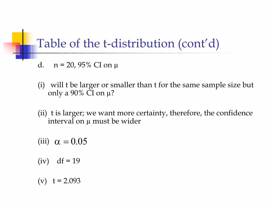
Table of the t-distribution (cont’d)d. n = 20, 95% CI on µ

(i) will t be larger or smaller than t for the same sample size but only a 90% CI on µ?

(ii) t is larger; we want more certainty, therefore, the confidence interval on µ must be wider

(iii)

(iv) df = 19

(v) t = 2.093

05.0=α

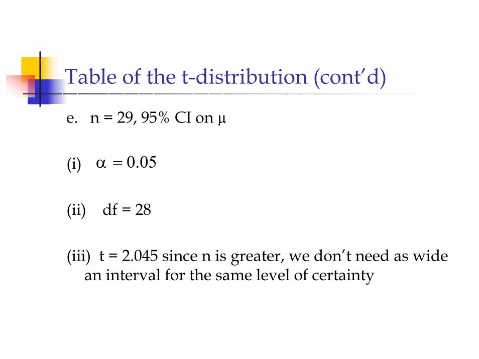
Table of the t-distribution (cont’d)

e. n = 29, 95% CI on µ

(i)

(ii) df = 28

(iii) t = 2.045 since n is greater, we don’t need as wide an interval for the same level of certainty

05.0=α

E. Computing CI’s on µ using Student’s t

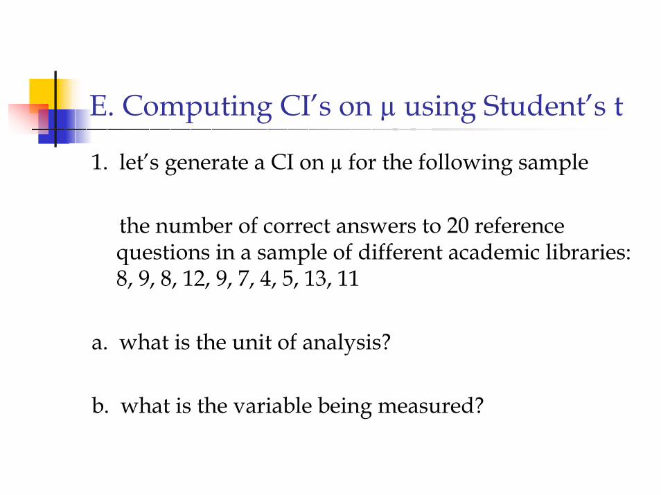
1. let’s generate a CI on µ for the following sample

the number of correct answers to 20 reference questions in a sample of different academic libraries: 8, 9, 8, 12, 9, 7, 4, 5, 13, 11

a. what is the unit of analysis?

b. what is the variable being measured?

Computing CI’s on µ using Student’s t (cont’d)

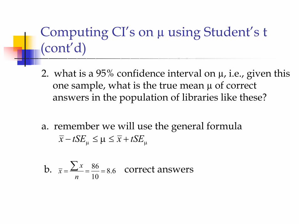
2. what is a 95% confidence interval on µ, i.e., given this one sample, what is the true mean µ of correct answers in the population of libraries like these?

a. remember we will use the general formula

b. correct answers

µµ µ tSExtSEx +≤≤−

6.81086

=== ∑nx

x

Computing CI’s on µ using Student’s t (cont’d)

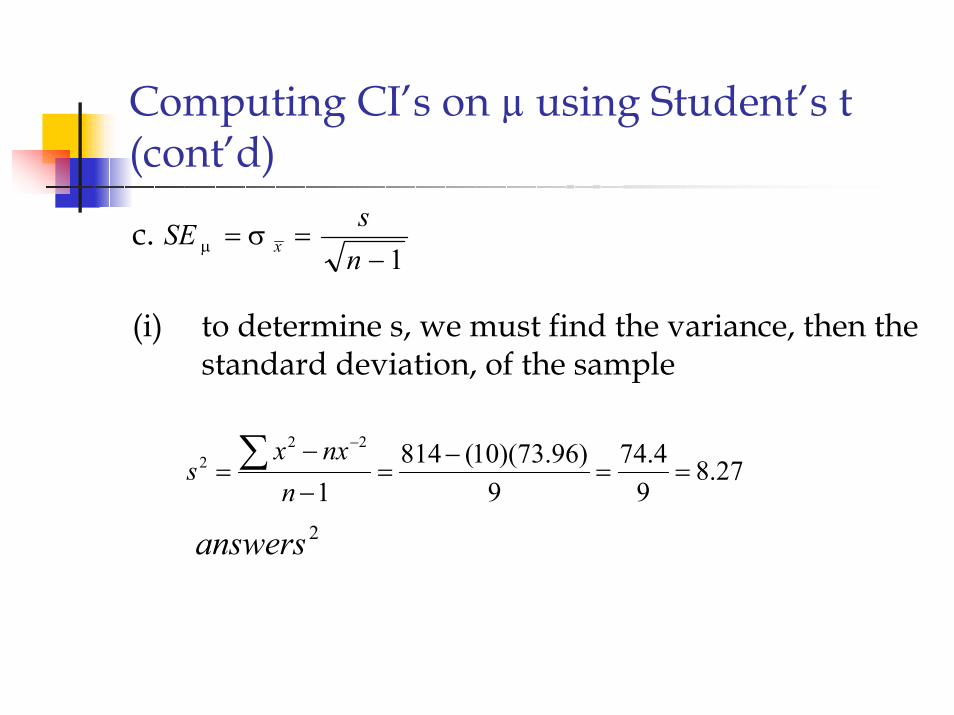
c.

(i) to determine s, we must find the variance, then the standard deviation, of the sample

1−==

nsSE xσµ

27.89

4.749

)96.73)(10(8141

222 ==

−=

−−

= ∑−

nnxx

s

2answers

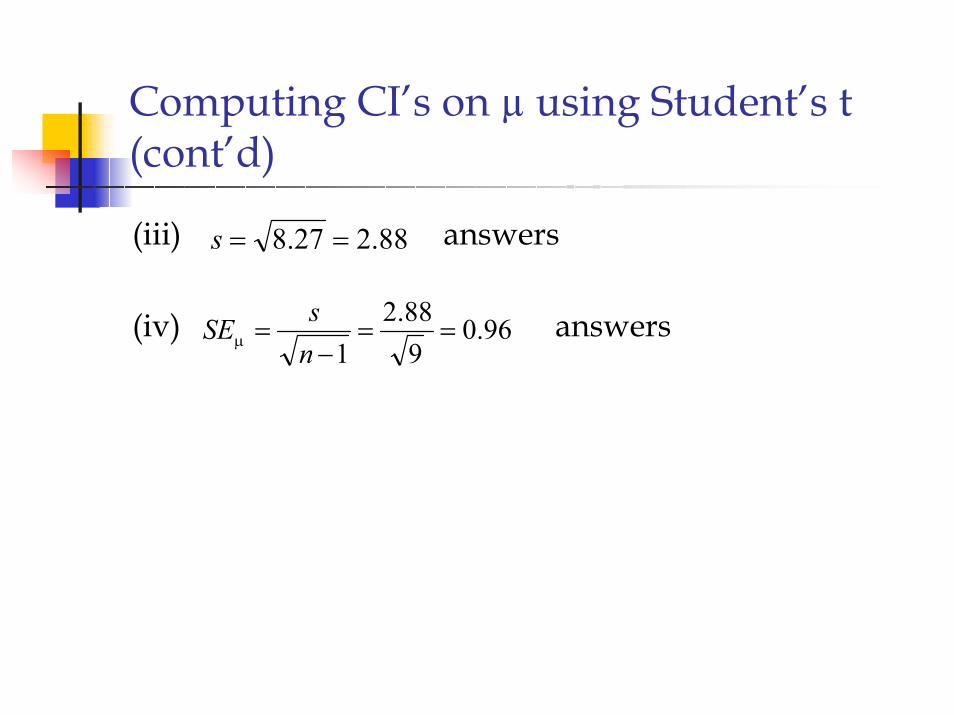
Computing CI’s on µ using Student’s t (cont’d)

(iii) answers

(iv) answers96.088.2===

sSEµ

88.227.8 ==s

91−n

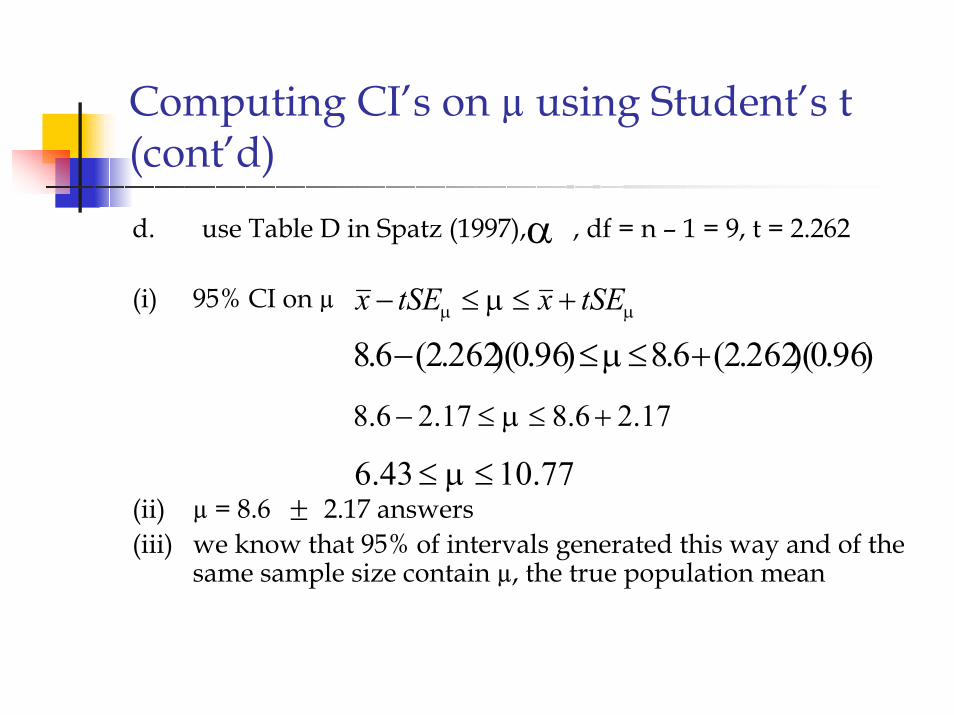
Computing CI’s on µ using Student’s t (cont’d)d. use Table D in Spatz (1997), , df = n – 1 = 9, t = 2.262

(i) 95% CI on µ

(ii) µ = 8.6 2.17 answers(iii) we know that 95% of intervals generated this way and of the

same sample size contain µ, the true population mean

α

µµ µ tSExtSEx +≤≤−

)96.0)(262.2(6.8)96.0)(262.2(6.8 +≤≤− µ

17.26.817.26.8 +≤≤− µ

77.1043.6 ≤≤ µ±

Computing CI’s on µ using Student’s t (cont’d)

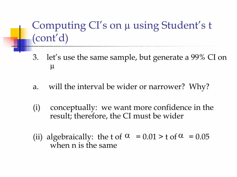
3. let’s use the same sample, but generate a 99% CI on µ

a. will the interval be wider or narrower? Why?

(i) conceptually: we want more confidence in the result; therefore, the CI must be wider

(ii) algebraically: the t of = 0.01 > t of = 0.05 when n is the same

α α

Computing CI’s on µ using Student’s t (cont’d)

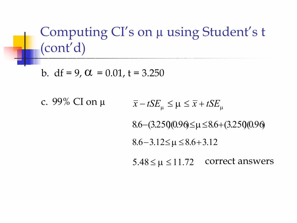
b. df = 9, = 0.01, t = 3.250

c. 99% CI on µ

correct answers

α

µµ µ tSExtSEx +≤≤−

)96.0)(250.3(6.8)96.0)(250.3(6.8 +≤≤− µ

12.36.812.36.8 +≤≤− µ

72.1148.5 ≤≤ µ

Computing CI’s on µ using Student’s t (cont’d)

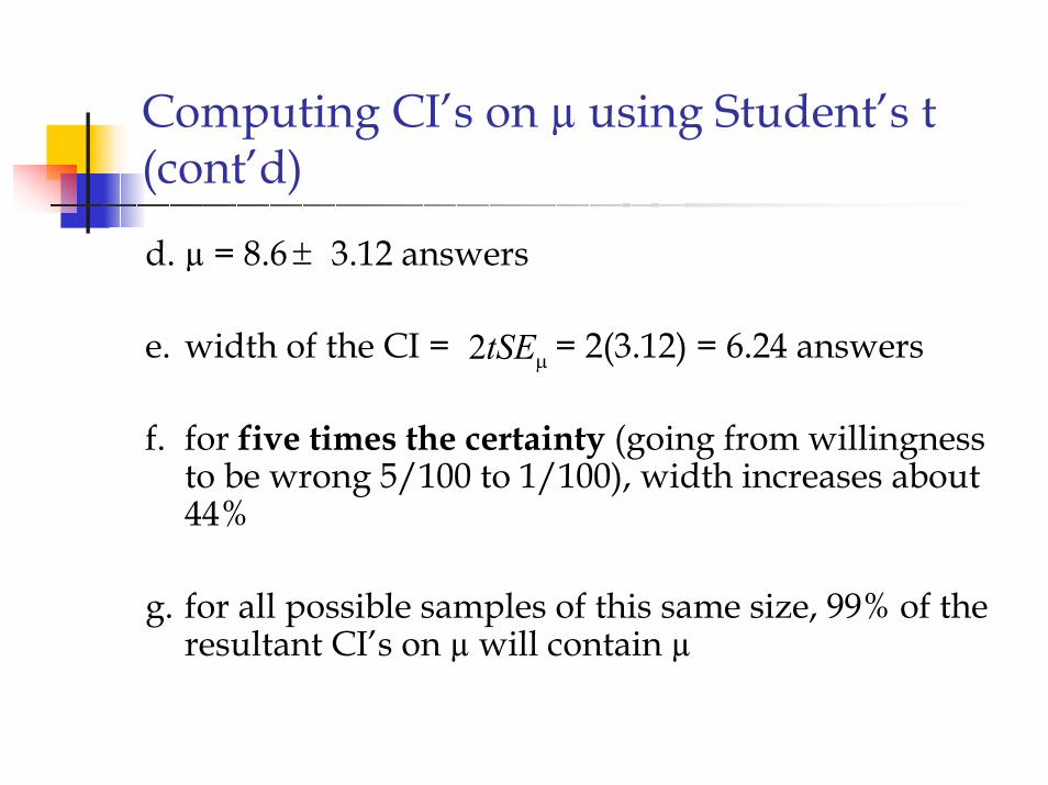
d. µ = 8.6 3.12 answers

e. width of the CI = = 2(3.12) = 6.24 answers

f. for five times the certainty (going from willingness to be wrong 5/100 to 1/100), width increases about 44%

g. for all possible samples of this same size, 99% of the resultant CI’s on µ will contain µ

±

µtSE2

F. Summary

1. Refer to Spatz (1997, p. 152, Figure 6.8)

2. remember that a confidence interval on µ identifies a “range of values within which a population parameter [in this case, the true population mean] is estimated to lie” over all possible samples at a particular level of confidence (Babbie, 1998, G2).