STAT COE-Report-08-2016

STAT T&E Center of Excellence 2950 Hobson Way – Wright-Patterson AFB, OH 45433

Confidence Intervals for the Median and Other Percentiles

Best Practice

Authored by: Sarah Burke, Ph.D. STAT T&E COE

12 December 2016

The goal of the STAT T&E COE is to assist in developing rigorous, defensible test strategies to

more effectively quantify and characterize system performance and provide information that

reduces risk. This and other COE products are available at www.AFIT.edu/STAT.

STAT COE-Report-08-2016

Table of Contents

Executive Summary ....................................................................................................................................... 2

Introduction .................................................................................................................................................. 2

Definitions and Notation ............................................................................................................................... 2

Estimating Percentiles ................................................................................................................................... 3

Finding the Confidence Limits Using JMP ..................................................................................................... 3

Alternate Approaches ................................................................................................................................... 7

Conclusion ..................................................................................................................................................... 7

References .................................................................................................................................................... 7

Appendix ....................................................................................................................................................... 8

STAT COE-Report-08-2016

Page 2

Executive Summary This best practice explains an approach to construct confidence intervals for the median and

other percentiles by walking through an example in JMP. When the distribution of a statistic for a

population characteristic of interest is known, we can use the properties of this distribution to construct

confidence intervals of that population characteristic. For example, if the population has a normal

distribution, then the sample mean has a normal distribution and we use this information to construct

confidence intervals of the population mean. The construction of construct confidence intervals for the

median, or other percentiles, however, is not as straightforward.

Keywords: confidence interval, median, percentile, statistical inference

Introduction Kensler and Cortes (2014) and Ortiz and Truett (2015) discuss the use and interpretation of

confidence intervals (CIs) to draw conclusions about some characteristic of a population. These best

practices provide examples of CIs for a population proportion and population mean, respectively. In this

best practice, let us assume that our characteristic of interest is a continuous variable. If we know that

the underlying distribution of this variable is normally distributed, we can use the techniques discussed

by Ortiz and Truett (2015) to calculate a CI from a random sample of data from our population.

However, what is the correct approach when the assumptions required for the CI do not apply?

If the assumptions of CIs for the mean do not hold for your data or the distribution of your

population is unknown, it may be advantageous to estimate the median. There may also be cases where

a percentile (for example the 75th or 95th percentile) may be of more interest than the center of the

data. We can easily calculate an estimate of the population percentiles from a random sample (see

below). However, this is a point estimate: a single value that estimates the population percentile. Rather

than provide only a single value, we would like to also determine a confidence interval on the

population percentile. This would provide us a realistic range of values for the percentile with a given

degree of confidence. In this best practice, we demonstrate how to determine CIs of population

percentiles, including the median. The technique is demonstrated using JMP (V.12). The appendix

provides the mathematical details for those interested.

Definitions and Notation We first introduce some definitions and notation to explain the method of constructing CIs for

percentiles.

Percentile: The pth percentile (denoted 𝑥𝑝) is the value 𝑥 of a population/random variable such that

P(𝑋 ≤ 𝑥) = 𝑝. The pth (sample) percentile (denoted 𝑥𝑝) is the value such that 100𝑝% of the sample is

smaller than 𝑥. Equivalently, 100(1 − 𝑝)% of the data lies above 𝑥 (Kvam and Vidakovic, 2007). The

STAT COE-Report-08-2016

Page 3

median, for example, is the 50th percentile. 50% of the population falls below the median and 50% lies

above the median. The 75th percentile, 𝑥0.75, is the value such that 75% of the population falls below

𝑥0.75 and 25% lies above 𝑥0.75.

Order Statistic: Let 𝑋1, 𝑋2, … , 𝑋𝑛 be a random, independent sample from a population. The sample can

be ordered in an ascending order and denoted as 𝑋(1), 𝑋(2), … , 𝑋(𝑛) such that:

𝑋(1) < 𝑋(2) < ⋯ < 𝑋(𝑛−1) < 𝑋(𝑛)

where 𝑋(𝑖) denotes the 𝑖th largest value in the sample. So, for example, 𝑋(1) denotes the minimum and

𝑋(𝑛) denotes the maximum. 𝑋(𝑖) is called an order statistic. Order statistics are commonly used in

nonparametric statistics, a field of statistics that does not rely on assumptions of the distribution of the

population. (A side note: nonparametric statistics does not mean “assumption-free!”) We can use order

statistics to determine a confidence interval for the median of a population (or any other percentile).

There are many theoretical properties regarding order statistics (see Kvam and Vidakovic, 2007 or

Casella and Berger, 2002 for details).

Estimating Percentiles

For large samples, there is often a rank number 𝑟 between 1 and the sample size 𝑛 such that

𝑋(𝑟) = 𝑥𝑝. In other words, a value in the sample is the pth percentile if 𝑝(𝑛 + 1) = 𝑟 (Kvam and

Vidakovic, 2007). For example, a random sample of 5 observations has the values 4, 2, 7, 5, 9. Arranging

this sample in ascending order gives us 2, 4, 5, 7, 9. The 50th percentile (the median) corresponds to the

3rd order statistic 𝑋(3) = 5 since 0.5(5 + 1) = 𝑟 = 3. However, note that if we wish to estimate the 75th

percentile in this way, there is not an integer 𝑟 between 1 and 𝑛 such that 0.75(5 + 1) = 𝑟.

If 𝑝(𝑛 + 1) is not an integer, we can interpolate the percentile between 𝑋(𝑟) and 𝑋(𝑟+1), often

done with software. For example, if the sample size is even, the median can be estimated as 𝑀 =𝑋(𝑛)+𝑋(𝑛+1)

2. If your sample size is odd, the median can be estimated as 𝑀 = 𝑋

(𝑛+1

2), as we saw above.

Finding the Confidence Limits Using JMP The previous section explained how to estimate a percentile with a single value. The goal is to

identify values 𝑋(𝑗) and 𝑋(𝑘) in the sample such that P(𝑋(𝑗) ≤ 𝑥𝑝 ≤ 𝑋(𝑘)) = 1 − 𝛼, where 𝛼 denotes

the probability of a type I error and 1 − 𝛼 denotes the confidence level. For example,

P(𝑋(𝑗) ≤ 𝑥0.50 ≤ 𝑋(𝑘)) = 0.95 would provide us a 95% CI of the population median using values

contained in the sample. Note how this approach is different compared to CIs for the mean and

proportion discussed previously. Those approaches take on the general form of:

𝑠 = 𝐶(𝑐𝑜𝑛𝑓 𝑙𝑒𝑣𝑒𝑙,𝑛)𝑠. 𝑒. (𝑠),

STAT COE-Report-08-2016

Page 4

where 𝑠 is some statistic, 𝐶 is a critical value based on the confidence level and sample size, and 𝑠. 𝑒. (𝑠)

is the standard error of the statistic. This is a parametric approach, meaning it uses properties of the

distribution of the statistic to determine the lower and upper confidence bounds. CIs for percentiles

uses a nonparametric approach, which, as mentioned previously, does not use any information about

the distribution of the statistic. Therefore, this approach uses the data contained in the sample to

determine lower and upper confidence bounds for the population percentile.

Let’s consider an example. Suppose we have the following random sample of size 20 from some

population with an unknown distribution (displayed in Table 1). For convenience, the data are listed in

ranked (ascending) order.

Table 1. Random Sample of Data (in Ascending Order)

Rank 1 2 3 4 5 6 7 8 9 10

Value 0.49 0.59 0.86 1.01 1.24 1.25 1.81 2.01 2.29 2.66

Rank 11 12 13 14 15 16 17 18 19 20

Value 2.82 2.85 3 3.27 4.44 5.14 5.53 5.6 6.06 6.29

What is a 95% CI for the median and the 75th percentile? Using statistical software, we can

estimate the median and 75th percentile and their respective CIs. To perform this analysis in JMP (V.12),

with your data opened in a data table, select “Distribution” under the “Analyze” menu. Select your

variable of interest in the “y” box, and click OK. In the results window, go to the red triangle, select

display options, and then select custom quantiles (Figure 1). Enter in the percentiles of interest (0.50 for

median, 0.25 for 25th percentile, 0.75 for 75th percentile, etc.) [see Figure 2]. The results are now

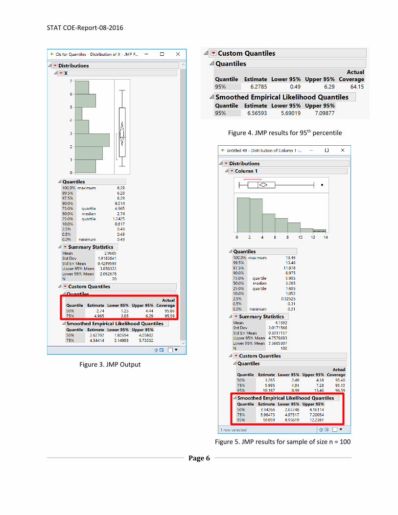
displayed in the distribution results window (Figure 3). JMP displays the point estimate for the median

as well as the lower and upper confidence limits. JMP also displays the actual confidence. As explained

in the Appendix, the actual confidence may not be equal to the desired confidence because the

approach uses the Binomial distribution (a discrete distribution) to determine which values in the

sample are the lower and upper confidence limits. Particularly when the sample size is small, the CIs

may have a much smaller level of confidence than desired.

As seen in Figure 3, the estimate of the median is 𝑥0.50 = 2.74. Note that this is equal to

(𝑋(10) + 𝑋(11)) 2⁄ = (2.66 + 2.82)/2 from Table 1. The JMP results show that the 95% CI for the

median is (1.25, 2.44) and the actual coverage is just above 95%. The estimate of the 75th percentile is

4.965 with an approximate 95% CI of (2.85, 6.29) which correspond to 𝑋(11) and 𝑋(20). The actual

coverage for this CI is also just above 95%.

Now suppose we wish to find a 95% CI for the 95th percentile of the population based on the

sample in Table 1. Figure 4 displays the JMP results for this scenario. The 95th percentile is estimated as

6.2785. The “95%” CI is (0.49, 6.29), which is the entire range of the sample data. Note that the actual

coverage is just 64.15%, much lower than the desired 95% confidence. Because this dataset is so small,

STAT COE-Report-08-2016

Page 5

using this approach does not yield a CI with the desired confidence level. Suppose we took a sample of

size 100 from the same population as the previous sample. The distribution analysis results from JMP

are shown in Figure 5. First note that this data is clearly not normally distributed. The 95% CIs for the

median, 75th, and 95th percentiles for this larger sample are more realistic and each have actual

confidence slightly larger than the desired confidence 95% (see Figure 5).

Figure 1. JMP Instructions Step 1

Figure 2. JMP Instructions Step

2

STAT COE-Report-08-2016

Page 6

Figure 3. JMP Output

Figure 4. JMP results for 95th percentile

Figure 5. JMP results for sample of size n = 100

STAT COE-Report-08-2016

Page 7

Alternate Approaches The mathematical details to determine the CIs for percentiles based on the distribution-free

method described above is explained in the Appendix. JMP also calculates “Smoothed Empirical

Likelihood Estimates” which is based on the work of Chen and Hall (1993). These results can be seen in

Figure 3 and Figure 5. This is a more advanced method to calculate CIs for percentiles that uses a

distribution constructed from the observed sample data. The method discussed previously was truly

distribution-free and only required determining which ranked values in the sample to use as the lower

and upper confidence bounds.

An alternate approach to finding CIs for percentiles (and any statistic) without relying on the

distribution of the population is to use bootstrapping. In short, bootstrapping is a resampling method to

estimate the sampling distribution of a statistic. The sampling distribution of the sample mean can be

approximated by the Central Limit Theorem. The sampling distributions of other statistics, however, are

often unknown (like with the median or other percentiles). To construct CIs on a statistic, we use

properties of the sampling distribution to determine the confidence bounds. When this distribution is

unknown, bootstrapping can estimate this sampling distribution which we can then use to construct the

CIs. Bootstrapping will be discussed in a separate Best Practice. See Givens and Hoeting (2013) for

details on bootstrapping.

Conclusion It is possible to calculate CIs for the median and other percentiles. A word of caution worth

reiterating: for small sample sizes, the method described here is not an ideal approach because of its

limitations. With small sample sizes, we are not guaranteed to get a CI with the desired confidence level,

particularly with the extreme percentiles (for example, 5% or 95% percentiles). It should also be noted

that if the assumptions for a CI for the mean are valid for your sample, the CI for the mean will be more

powerful than the method described here. When the assumptions are not valid however, or a percentile

is the population characteristic of interest, we can accompany the point estimate with a CI. This will give

us a realistic range of values for the population percentile of interest.

References Casella, G. and Berger, R. L. (2002) “Statistical Inference”, Duxbury Thomas Learning.

Chen, Song Xi and Hall, Peter. (1993) “Smoothed Empirical Likelihood Confidence Intervals for

Quantiles”, The Annals of Statistics, 21(3), 1166 – 1181.

Givens G. H. and Hoeting, J. A. (2013), Computational Statistics, Hoboken, NJ: John Wiley & Sons p. 287-

319.

STAT COE-Report-08-2016

Page 8

Hahn, G. J. and Meeker, W. Q. (1991), Statistical Intervals: A Guide for Practitioners, New York: John

Wiley & Sons.

JMP®, Version 12. SAS Institute Inc., Cary, NC, 1989-2007.

Kensler, J. and Cortes, L. (2014). A Practical Guide for Interpreting Confidence Intervals. Retrieved

December 7, 2016, from STAT in T&E Center of Excellence:

https://www.afit.edu/images/pics/file/A%20Practical%20Guide%20for%20Interpreting%20Confi

dence%20Intervals(2).pdf

Kvam, Paul H. and Vidakovic (2007). Nonparametric Statistics with Applications to Science and

Engineering, Hoboken, NJ: John Wiley & Sons.

Milefoot. http://www.milefoot.com/math/stat/ci-medians.htm. Accessed 7 December 2016.

Ortiz, F. and Truett, L. (2015). Using Statistical Intervals to Assess System Performance. Retrieved

December 7, 2016 from STAT in T&E Center of Excellence:

http://www.afit.edu/images/pics/file/BP%20-%20Statistical%20Intervals.pdf

Appendix Here we explain the derivation of the confidence limits for percentiles. Note that there are two

possible outcomes for each sample value 𝑋𝑖: it is either below the 100pth percentile or it’s not (a binary

outcome). The probability that a value falls below the 100pth percentile is p. Our sample size is fixed at n.

These conditions (along with our random sample assumption) gives us the conditions to apply the

Binomial distribution to determine the lower and upper confidence limits. The binomial distribution is a

common distribution for a discrete random variable and, for example, can be used to estimate the

number of successes (or failures) in 𝑛 trials. Therefore, a 100(1-𝛼)% CI that the 100pth percentile will fall

between the jth and kth order statistic 𝑋(𝑗) and 𝑋(𝑘) is (http://www.milefoot.com/math/stat/ci-

medians.htm):

P(𝑋(𝑗) ≤ 𝑥𝑝 ≤ 𝑋(𝑘−1)) = ∑𝑛!

(𝑛 − 𝑖)! 𝑖!𝑝𝑖(1 − 𝑝)𝑛−𝑖

𝑘−1

𝑖=𝑗

≈ 1 − 𝛼

Consider the sample data in Table 1 where we wanted to determine a 95% CI of the median.

Table 2 shows the probabilities for the binomial distribution for the median and the given sample size (n

= 20, p = 0.50). This table supplies the probabilities that the percentile falls in the 𝑖th subinterval of the

ranked data. For example, 𝑖 = 0 corresponds to the case where the pth population percentile falls below

the minimum in the sample, 𝑖 = 1 corresponds to the case where the percentile falls between the first

and second order statistics, and 𝑖 = 𝑛 corresponds to the case where the percentile is greater than the

maximum (see Figure 6 for a graphical representation of this up to 𝑖 = 5).

STAT COE-Report-08-2016

Page 9

Order statistic: 𝑋(1) 𝑋(2) 𝑋(3) 𝑋(4) 𝑋(5)

𝑖th subinterval: 0 1 2 3 4 5

Figure 1. Graphical Representation of Table 2

We want to find values 𝑋(𝑗) and 𝑋(𝑘−1) such that P(𝑋(𝑗) ≤ 𝑥0.50 ≤ 𝑋(𝑘−1)) ≈ 1 − 𝛼. The probabilities in

Table 2 are calculated from the binomial distribution such that:

𝑃(𝑋 = 𝑖) =𝑛!

(𝑛 − 𝑖)! 𝑖!𝑝𝑖(1 − 𝑝)𝑛−𝑖

Table 2. Binomial Probabilities for Median n = 20, p = 0.50

𝑋 = 𝑖 𝑃(𝑋 = 𝑖) 𝑋 = 𝑖 𝑃(𝑋 = 𝑖) 0 0 11 0.16018

1 0.00002 12 0.12013

2 0.00018 13 0.07393

3 0.00109 14 0.03696

4 0.00462 15 0.01479

5 0.01479 16 0.00462

6 0.03696 17 0.00109

7 0.07393 18 0.00018

8 0.12013 19 0.00002

9 0.16018 20 0.00000

10 0.1762

Table 3 sorts these probabilities from largest to smallest to identify the set of subintervals with the

desired confidence.

Table 3. Binomial Probabilities for Median n = 20, p= 0.50 (Sorted Descending)

𝑋 = 𝑖 𝑃(𝑋 = 𝑖) 𝑋 = 𝑖 𝑃(𝑋 = 𝑖) 10 0.1762 16 0.00462

11 0.16018 4 0.00462

9 0.16018 17 0.00109

12 0.12013 3 0.00109

8 0.12013 18 0.00018

13 0.07393 2 0.00018

7 0.07393 19 0.00002

14 0.03696 1 0.00002

6 0.03696 20 0.00000

15 0.01479

STAT COE-Report-08-2016

Page 10

Using Table 3, therefore, we can say:

P(𝑋(6) ≤ 𝑥𝑝 ≤ 𝑋(14)) = ∑𝑛!

(𝑛 − 𝑖)! 𝑖!𝑝𝑖(1 − 𝑝)𝑛−𝑖

14

𝑖=6

= 0.03696 + 0.07393 + 0.12013 + 0.16018 + 0.1762 + 0.16018 + 0.12013 + 0.07393 + 0.03696

= 0.9586

The confidence bounds for the 95% CI begin at the 6th subinterval (𝑋(6)) and end at the end of the 14th

subinterval (𝑋(15)). This yields a 95% (actually 95.86%) CI for the median of (𝑋(6), 𝑋(15)) = (1.25,4.44)

by referring to the ranked values in Table 1. Note that this matches the output from JMP in Figure 3.

Note also that because of the discrete nature of the binomial distribution, we may not be able to get a CI

with confidence exactly equal to 1 − 𝛼. And as discussed in the main text, for small sample sizes, the

actual confidence can be much lower than the desired confidence.