
Confidence intervals for low dimensional parameters in high dimensional linear models
26
© 2013 Royal Statistical Society 1369–7412/14/76217 J. R. Statist. Soc. B (2014) 76, Part 1, pp. 217–242 Confidence intervals for low dimensional parameters in high dimensional linear models Cun-Hui Zhang Rutgers University, Piscataway, USA and Stephanie S. Zhang Columbia University, New York, USA [Received October 2011. Final revision January 2013] Summary. The purpose of this paper is to propose methodologies for statistical inference of low dimensional parameters with high dimensional data. We focus on constructing confidence inter- vals for individual coefficients and linear combinations of several of them in a linear regression model, although our ideas are applicable in a much broader context. The theoretical results that are presented provide sufficient conditions for the asymptotic normality of the proposed estima- tors along with a consistent estimator for their finite dimensional covariance matrices. These sufficient conditions allow the number of variables to exceed the sample size and the presence of many small non-zero coefficients. Our methods and theory apply to interval estimation of a preconceived regression coefficient or contrast as well as simultaneous interval estimation of many regression coefficients. Moreover, the method proposed turns the regression data into an approximate Gaussian sequence of point estimators of individual regression coefficients, which can be used to select variables after proper thresholding. The simulation results that are presented demonstrate the accuracy of the coverage probability of the confidence intervals proposed as well as other desirable properties, strongly supporting the theoretical results. Keywords: Confidence interval; High dimension; Linear regression model; p-value; Statistical inference 1. Introduction The area of high dimensional data is an area of intense research in statistics and machine learning, owing to the rapid development of information technologies and their applications in scientific experiments and everyday life. Numerous large, complex data sets have been collected and are waiting to be analysed; meanwhile, an enormous effort has been mounted to meet this challenge by researchers and practitioners in statistics, computer science and other disciplines. A great number of statistical methods, algorithms and theories have been developed for the prediction and classification of future outcomes, the estimation of high dimensional objects and the selection of important variables or features for further scientific experiments and engineering applications. However, statistical inference with high dimensional data is still largely untouched, owing to the complexity of the sampling distributions of existing estimators. This is particularly Address for correspondence: Cun Hui Zhang, Department of Statistics and Biostatistics, Hill Center, Busch Campus, Rutgers University, Piscataway, NJ 08854, USA. E-mail: [email protected] Reuse of this article is permitted in accordance with the terms and conditions set out at http://wileyonline library.com/onlineopen#OnlineOpen Terms.
-
Upload
stephanie-s -
Category
Documents
-
view
213 -
download
0
Transcript of Confidence intervals for low dimensional parameters in high dimensional linear models
© 2013 Royal Statistical Society 1369–7412/14/76217
J. R. Statist. Soc. B (2014)76, Part 1, pp. 217–242
Confidence intervals for low dimensional parametersin high dimensional linear models
Cun-Hui Zhang
Rutgers University, Piscataway, USA
and Stephanie S. Zhang
Columbia University, New York, USA
[Received October 2011. Final revision January 2013]
Summary.The purpose of this paper is to propose methodologies for statistical inference of lowdimensional parameters with high dimensional data.We focus on constructing confidence inter-vals for individual coefficients and linear combinations of several of them in a linear regressionmodel, although our ideas are applicable in a much broader context.The theoretical results thatare presented provide sufficient conditions for the asymptotic normality of the proposed estima-tors along with a consistent estimator for their finite dimensional covariance matrices. Thesesufficient conditions allow the number of variables to exceed the sample size and the presenceof many small non-zero coefficients. Our methods and theory apply to interval estimation of apreconceived regression coefficient or contrast as well as simultaneous interval estimation ofmany regression coefficients. Moreover, the method proposed turns the regression data intoan approximate Gaussian sequence of point estimators of individual regression coefficients,which can be used to select variables after proper thresholding. The simulation results that arepresented demonstrate the accuracy of the coverage probability of the confidence intervalsproposed as well as other desirable properties, strongly supporting the theoretical results.
Keywords: Confidence interval; High dimension; Linear regression model; p-value; Statisticalinference
1. Introduction
The area of high dimensional data is an area of intense research in statistics and machinelearning, owing to the rapid development of information technologies and their applications inscientific experiments and everyday life. Numerous large, complex data sets have been collectedand are waiting to be analysed; meanwhile, an enormous effort has been mounted to meet thischallenge by researchers and practitioners in statistics, computer science and other disciplines.A great number of statistical methods, algorithms and theories have been developed for theprediction and classification of future outcomes, the estimation of high dimensional objects andthe selection of important variables or features for further scientific experiments and engineeringapplications. However, statistical inference with high dimensional data is still largely untouched,owing to the complexity of the sampling distributions of existing estimators. This is particularly
Address for correspondence: Cun Hui Zhang, Department of Statistics and Biostatistics, Hill Center, BuschCampus, Rutgers University, Piscataway, NJ 08854, USA.E-mail: [email protected]
Reuse of this article is permitted in accordance with the terms and conditions set out at http://wileyonlinelibrary.com/onlineopen#OnlineOpen Terms.
218 C.-H. Zhang and S. S. Zhang
so in the context of the so-called large p smaller n problem, where the dimension of the data p
is greater than the sample size n.Regularized linear regression is one of the best understood statistical problems in high
dimensional data. Important work has been done in problem formulation, methodology andalgorithm development, and theoretical analysis under sparsity assumptions on the regres-sion coefficients. This includes l1 regularized methods (Tibshirani, 1996; Chen et al., 2001;Greenshtein and Ritov, 2004; Greenshtein, 2006; Meinshausen and Buhlmann, 2006; Tropp,2006; Zhao and Yu, 2006; Candes and Tao, 2007; Zhang and Huang, 2008; Bickel et al., 2009;Koltchinskii, 2009; Meinshausen and Yu, 2009; van de Geer and Buhlmann, 2009; Wainwright,2009a; Zhang, 2009; Ye and Zhang, 2010; Koltchinskii et al., 2011; Sun and Zhang, 2010),non-convex penalized methods (Frank and Friedman, 1993; Fan and Li, 2001; Fan and Peng,2004; Kim et al., 2008; Zhang, 2010; Zhang and Zhang, 2012), greedy methods (Zhang, 2011a),adaptive methods (Zou, 2006; Huang et al., 2008; Zhang, 2011b; Zhang and Zhang, 2012),screening methods (Fan and Lv, 2008), and more. For further discussion, we refer to relatedsections in Buhlmann and van de Geer (2011) and recent reviews in Fan and Lv (2010) andZhang and Zhang (2012).
Among existing results, variable selection consistency is most relevant to statistical inference.In an l0 sparse setting, an estimator is variable selection consistent if it selects the oracle modelcomposed of exactly the set of variables with non-zero regression coefficients. In the large psmaller n setting, variable selection consistency has been established under incoherence andother l∞-type conditions on the design matrix for the lasso (Meinshausen and Buhlmann,2006; Tropp, 2006; Zhao and Yu, 2006; Wainwright, 2009a), and under sparse eigenvalue orl2-type conditions for non-convex methods (Zhang, C. H., 2010; Zhang, T., 2011a,b; Zhangand Zhang, 2012). Another approach in variable selection with high dimensional data involvessubsampling or randomization, including notably the stability selection method (Meinshausenand Buhlmann, 2010). Since the oracle model is typically assumed to be of smaller order indimension than the sample size n in selection consistency theory, consistent variable selectionallows a great reduction of the complexity of the analysis from a large p smaller n problemto a problem involving the oracle set of variables only. Consequently, taking the least squaresestimator on the selected set of variables if necessary, statistical inference can be justified in thesmaller oracle model.
However, statistical inference based on selection consistency theory typically requires a uni-form signal strength condition that all non-zero regression coefficients be greater in magnitudethan an inflated level of noise to take model uncertainty into account. This inflated level of noisecan be written as Cσ
√{.2=n/ log.p/}, where σ is the level of noise. It follows from Fano’s lemma(Fano, 1961) that C � 1
2 is required for variable selection consistency with a general standard-ized design matrix (Wainwright, 2009b; Zhang, 2010). This uniform signal strength condition is,unfortunately, seldom supported by either the data or the underlying science in applications whenthe presence of weak signals cannot be ruled out. In such cases, consistent estimation of thedistribution of the least squares estimator after model selection is impossible (Leeb and Potscher,2006). Conservative statistical inference after model selection or classification has been consid-ered in Berk et al. (2010) and Laber and Murphy (2011). However, such conservative methodsmay not yield sufficiently accurate confidence regions or p-values for common applications witha large number of variables.
We propose a low dimensional projection (LDP) approach to constructing confidenceintervals for regression coefficients without assuming the uniform signal strength condition. Weprovide theoretical justifications for the use of the proposed confidence interval for a precon-ceived regression coefficient or a contrast depending on a small number of regression coefficients.
Confidence Intervals for Low Dimensional Parameters 219
We believe that, in the presence of potentially many non-zero coefficients of small or moderatemagnitude, construction of a confidence interval for such a preconceived parameter is animportant problem in and of itself and was open before our paper (Leeb and Potscher, 2006),but the method proposed is not limited to this application.
Our theoretical work also justifies the use of LDP confidence intervals simultaneously aftera multiplicity adjustment, in the absence of a preconceived parameter of interest. Moreover, athresholded LDP estimator can be used to select variables and to estimate the entire vector ofregression coefficients.
The most important difference between the LDP and existing variable selection approachesconcerns the requirement of the uniform signal strength condition, as we have mentioned earlier.This is a necessity for the simultaneous correct selection of all zero and non-zero coefficients.If this criterion is the goal, we cannot do better than technical improvements over existingmethods. However, a main complaint about the variable selection approach is the practicalityof the uniform signal strength condition, and the crucial difference between the two approaches isprecisely in the case where the condition fails to hold. Without the condition, the LDP approachis still able to select correctly all coefficients above a threshold of order C
√{.2=n/ log.p/} and allzero coefficients. The power of the LDP method is small for testing small non-zero coefficients,but this is unavoidable and does not affect the correct selection of other variables. In this sense, theconfidence intervals proposed decompose the variable selection problem into multiple marginaltesting problems for individual coefficients as Gaussian means.
Most results presented here are available through Zhang and Zhang (2011). Proofs for thecurrent paper are provided in the on-line supplement.
2. Methodology
We develop methodologies and algorithms for the construction of confidence intervals for theindividual regression coefficients and their linear combinations in the linear model
y=Xβ+ε, ε∼N .0, σ2I/, .1/
where y∈Rn is a response vector, X= .x1, : : : , xp/∈Rn×p is a design matrix with columns xj andβ= .β1, : : : , βp/T is a vector of unknown regression coefficients. When rank.X/<p, β is uniqueunder proper conditions on the sparsity of β, but not in general. To simplify the discussion,we standardize the design to ‖xj‖22= n. The design matrix X is assumed to be deterministicthroughout the paper, except in Section 3.5.
The following notation will be used. For real numbers x and y, x∧ y=min.x, y/, x∨ y=max.x, y/, x+=x∨0 and x−= .−x/+. For vectors v= .v1, : : : , vm/ of any dimension, supp.v/={j : vj = 0}, ‖v‖0= |supp.v/| =#{j : vj = 0} and ‖v‖q= {Σj |vj|q/1=q, with the usual extensionto q=∞. For A⊂{1, : : : , p}, vA= .vj, j∈A/T and XA= .xk, k∈A/, including A=−j={1, : : : ,p}\{j}.
2.1. Bias-corrected linear estimatorsIn the classical theory of linear models, the least squares estimator of an estimable regressioncoefficient βj can be written as
β.lse/
j := .x⊥j /Ty=.x⊥j /Txj, .2/
where x⊥j is the projection of xj to the orthogonal complement of the column space of X−j=.xk, k = j/. Since this is equivalent to solving the equations .x⊥j /T.y−βjxj/ in the score system

220 C.-H. Zhang and S. S. Zhang
v→ .x⊥j /Tv, x⊥j can be viewed as the score vector for the least squares estimation of βj. Thescore vector x⊥j can be defined by .x⊥j /Txk= 0 ∀k = j and .x⊥j /Txj =‖x⊥j ‖22. For estimable βj
and βk,
cov.β.lse/
j , β.lse/
k /=σ2.x⊥j /Tx⊥k =.‖x⊥j ‖22‖x⊥k ‖22/: .3/
In the high dimensional setting p>n, rank.X−j/=n for all j when X is in general position. Inthis case x⊥j =0 and estimator (2) is undefined. However, it may still be interesting to preservecertain properties of the least squares estimator. This can be done by retaining the main equationzT
j .y− βjxj/= 0 in a score system zj : v→ zTj v and relaxing the constraint zT
j xk = 0 for k =j, resulting in a linear estimator. For any score vector zj that is not orthogonal to xj, thecorresponding univariate linear regression estimator satisfies
β.lin/
j = zTj y
zTj xj
=βj+zT
j ε
zTj xj
+∑k =j
zTj xkβk
zTj xj
:
The estimator consequently has a covariance structure of form (3). A problem with the newsystem is its bias. For every k = j with zT
j xk =0, the contribution of βk to the bias is linear in βk.Thus, under the assumption ‖β‖0 �2, which is very strong, the bias of β
.lin/j is still unbounded
when zTj xk = 0 for at least one k = j. We note that, for rank.X−j/=n, it is impossible to have
zj =0 and zTj xk=0 for all k = j, so bias is unavoidable. Nevertheless, this simple analysis of the
linear estimator suggests a bias correction with a non-linear initial estimator β.init/:
βj= β.lin/
j −∑k =j
zTj xkβ
.init/k
zTj xj
= zTj y
zTj xj
−∑k =j
zTj xkβ
.init/k
zTj xj
: .4/
We may also interpret equation (4) as a one-step self-bias correction from the initial estimatorand write
βj := β.init/j + zT
j .y−Xβ.init/
/=zTj xj:
The estimation error of equation (4) can be decomposed as a sum of the noise and theapproximation errors:
βj−βj=zT
j ε
zTj xj
+
∑k =j
zTj xk.βk− β
.init/k /
zTj xj
: .5/
We require that zj be a vector depending on X only, so that zTj ε=‖zj‖2∼N.0, σ2/. A full descrip-
tion of equation (4) still requires the specification of the score vector zj and the initial estimatorβ
.init/. These choices will be discussed in the following two subsections.
2.2. Low dimensional projectionsWe propose to use as zj a relaxed orthogonalization of xj against other design vectors. Recallthat zj aims to play the role of x⊥j , the projection of xj to the orthogonal complement of thecolumn space of X−j= .xk, k =j/. In the trivial case where ‖x⊥j ‖2 is not too small, we may simplytake zj=x⊥j . In addition to the case of rank.X−j/=n, in which x⊥j =0, a relaxed projection maybe useful when ‖x⊥j ‖2 is positive but small. Since a relaxed projection zj is used and estimator(4) is a bias-corrected projection of y in the direction of zj, hereafter we call estimator (4) thelow dimensional projection estimator (LDPE) for easy reference.
A proper relaxed projection zj should control both the noise and the approximation error
Confidence Intervals for Low Dimensional Parameters 221
terms in equation (5), given suitable conditions on {X, β} and an initial estimator β.init/. Theapproximation error of the LDPE (4) can be controlled by bounding the numerator of the biasterm in equation (5) as follows:∣∣∣∣ ∑
k =j
zTj xk.βk− β
.init/k /
∣∣∣∣�(
maxk =j|zT
j xk|)‖β.init/−β‖1: .6/
This conservative bound is conveniently expressed as the product of a known function of zj andthe initial estimation error independent of j. For score vectors zj, define
ηj=maxk =j|zT
j xk|=‖zj‖2,
τj=‖zj‖2=|zTj xj|:
.7/
We refer to ηj as the bias factor since ηj‖β.init/ −β‖1 controls the approximation error inconstraint (6) relative to the length of the score vector. We refer to τj as the noise factor, sinceτjσ is the standard deviation of the noise component in equation (5). Since zT
j ε∼N.0, σ2‖zj‖22/,equation (5) yields
ηj‖β.init/−β‖1=σ=o.1/⇒ τ−1j .βj−βj/≈N.0, σ2/: .8/
Thus, we would like to pick a zj with a small ηj for the asymptotic normality and a small τj
for efficiency of estimation. Confidence intervals for βj and linear functionals of them can beconstructed subject to condition (8) and a consistent estimator of σ.
We still need a suitable zj, a relaxed orthogonalization of xj against other design vectors.When the unrelaxed x⊥j is non-zero, it can be viewed as the residual of the least squares fit of xj
on X−j. A familiar relaxation of the least squares method is the addition of an l1-penalty. Thisleads to the choice of zj as the residual of the lasso. Let γj be the vector of coefficients from thelasso regression of xj on X−j. The lasso-generated score is
zj=xj−X−jγj, γj=arg minb
{‖xj−X−jb‖22
2n+λj‖b‖1
}: .9/
It follows from the Karush–Kuhn–Tucker conditions for equation (9) that |xTk zj=n|�λj for all
k = j, so expression (7) holds with ηj �nλj=‖zj‖2. This gives many choices of zj with different{ηj, τj}. Explicit choices of such a zj, or equivalently a λj, are described in the next subsection.A rationale for the use of a common penalty level λj for all components of b in equation (9) isthe standardization of all design vectors. In an alternative in Section 2.4, called the restrictedLDPE (RLDPE), the penalty is set to 0 for certain components of b in equation (9).
2.3. Implementation of the low dimensional projection estimatorWe must pick β.init/, σ, and the λj in equation (9). Since consistent estimation of σ and fullyautomatic choices of λj are needed, we use methods based on the scaled lasso and the leastsquares estimator after model selection by the scaled lasso (called the scaled lasso–LSE method).We outline the basic ideas and specific implementations in Table 1.
The scaled lasso (Antoniadis, 2010; Sun and Zhang, 2010, 2012) is a joint convex minimizationmethod given by
{β.init/
, σ}=arg minb,σ
{‖y−Xb‖22
2σn+ σ
2+λ0‖b‖1
}, .10/

222 C.-H. Zhang and S. S. Zhang
Table 1. LDPE .1�α/% confidence intervals for a preconceived βj
Step Idea Specific implementation
1 Find an initial estimate β.init/
of the Scaled lasso (10) or least squares estimatorentire β and a consistent estimate σ after scaled lasso selection (11)
2 Find zj as an approximate projection Residuals, with small bias and noiseof xj to X−j in the sense of near factors (7), in lasso regression of xjorthogonality to each xk , k = j against X−j (Table 2)
3 Calculate the LDPE βj bias correction βj= β.init/j + zT
j .y−Xβ.init//=zTj xj
by projecting the residual of β.init/ to zj
4 Calculate the noise factor τj τj=‖zj‖2=|zTj xj |
5 Calculate the LDPE confidence interval βj±Φ−1.1−α=2/στj
with a preassigned penalty level λ0. It automatically provides an estimate of the noise level inaddition to the initial estimator of β. We use λ0=λuniv=
√{.2=n/ log.p/} in our simulationstudy. Existing error bounds for the estimation of both β and σ require λ0=A
√{.2=n/ log.p=ε/}with certain A> 1 and 0 < ε�1 (Sun and Zhang, 2012).
Estimator (10) has appeared in the literature in different forms. The joint minimization for-mulation was given in Antoniadis (2010), and an equivalent algorithm in Sun and Zhang (2010).If the minimum over b is taken first in equation (10), the resulting σ appeared earlier in Zhang(2010). The square-root lasso (Belloni et al., 2011) gives the same β.init/ with a different formu-lation, but not joint estimation of σ. In addition, the formulations in Zhang (2010) and Sun andZhang (2010) allow concave penalties and a degrees-of-freedom adjustment.
Like the lasso, the scaled lasso is biased. An alternative initial estimator of {β, σ} can beproduced by applying least squares after scaled lasso selection. Let S
.scl/be the set of non-zero
estimated coefficients produced by the scaled lasso. When S.scl/
catches most large |βj|, the biasof estimator (10) can be reduced by the least squares estimator in the selected model S
.scl/and
the corresponding degrees of freedom adjusted estimate of σ:
{β.init/
, σ}=arg minb,σ
{‖y−Xb‖22
2σ max.n−|S.scl/|, 1/+ σ
2: bj=0 ∀j ∈ S
.scl/}
: .11/
This defines the scaled lasso–LSE estimator. We use the same notation in equations (10) and (11)since they both give initial estimates for the LDPE (4) and a noise level estimator for statisticalinference based on the LDPE. The specific estimators will henceforth be referred to by theirnames or as estimators (10) and (11). The scaled lasso–LSE estimator enjoys similar analyticalerror bounds to those of the scaled lasso and outperformed the scaled lasso in a simulationstudy (Sun and Zhang, 2012).
The scaled lasso can be also used to determine λj for the zj in equation (9). However, thepenalty level for the scaled lasso, set to guarantee performance bounds for the estimation ofregression coefficients and noise level, may not be the best for controlling the bias and thestandard error of the LDPE. By equations (7) and (8), it suffices to find a zj with a small biasfactor ηj and small noise factor τj. These quantities always can be easily computed. This isquite different from the estimation of {β, σ} in equation (10) in which the effect of overfittingis unobservable.
We chooseλj by trackingηj and τj in the lasso path. One of our ideas is to reduceηj by allowingsome overfitting of xj as long as τj is reasonably small. Ideally, this slightly more conservative
Confidence Intervals for Low Dimensional Parameters 223
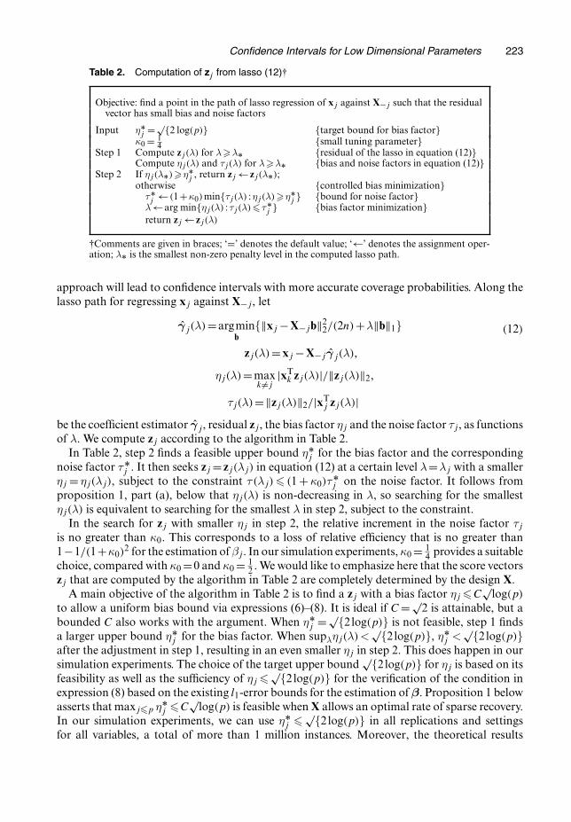
Table 2. Computation of zj from lasso (12)†
Objective: find a point in the path of lasso regression of xj against X−j such that the residualvector has small bias and noise factors
Input ηÅj =√{2 log.p/} {target bound for bias factor}
κ0= 14 {small tuning parameter}
Step 1 Compute zj.λ/ for λ�λÅ {residual of the lasso in equation (12)}Compute ηj.λ/ and τj.λ/ for λ�λÅ {bias and noise factors in equation (12)}
Step 2 If ηj.λÅ/�ηÅj , return zj← zj.λÅ/;
otherwise {controlled bias minimization}τÅj ← .1+κ0/min{τj.λ/ :ηj.λ/�ηÅ
j } {bound for noise factor}λ←arg min{ηj.λ/ : τj.λ/� τÅ
j } {bias factor minimization}return zj← zj.λ/
†Comments are given in braces; ‘=’ denotes the default value; ‘←’ denotes the assignment oper-ation; λÅ is the smallest non-zero penalty level in the computed lasso path.
approach will lead to confidence intervals with more accurate coverage probabilities. Along thelasso path for regressing xj against X−j, let
γj.λ/=argminb
{‖xj−X−jb‖22=.2n/+λ‖b‖1} .12/
zj.λ/=xj−X−jγj.λ/,
ηj.λ/=maxk =j|xT
k zj.λ/|=‖zj.λ/‖2,
τj.λ/=‖zj.λ/‖2=|xTj zj.λ/|
be the coefficient estimator γj, residual zj, the bias factor ηj and the noise factor τj, as functionsof λ. We compute zj according to the algorithm in Table 2.
In Table 2, step 2 finds a feasible upper bound ηÅj for the bias factor and the corresponding
noise factor τÅj . It then seeks zj= zj.λj/ in equation (12) at a certain level λ=λj with a smaller
ηj = ηj.λj/, subject to the constraint τ .λj/ � .1+ κ0/τÅj on the noise factor. It follows from
proposition 1, part (a), below that ηj.λ/ is non-decreasing in λ, so searching for the smallestηj.λ/ is equivalent to searching for the smallest λ in step 2, subject to the constraint.
In the search for zj with smaller ηj in step 2, the relative increment in the noise factor τj
is no greater than κ0. This corresponds to a loss of relative efficiency that is no greater than1−1=.1+κ0/2 for the estimation of βj. In our simulation experiments, κ0= 1
4 provides a suitablechoice, compared with κ0=0 and κ0= 1
2 . We would like to emphasize here that the score vectorszj that are computed by the algorithm in Table 2 are completely determined by the design X.
A main objective of the algorithm in Table 2 is to find a zj with a bias factor ηj �C√
log.p/
to allow a uniform bias bound via expressions (6)–(8). It is ideal if C=√2 is attainable, but abounded C also works with the argument. When ηÅ
j =√{2log.p/} is not feasible, step 1 finds
a larger upper bound ηÅj for the bias factor. When supληj.λ/ <
√{2log.p/}, ηÅj <√{2log.p/}
after the adjustment in step 1, resulting in an even smaller ηj in step 2. This does happen in oursimulation experiments. The choice of the target upper bound
√{2log.p/} for ηj is based on itsfeasibility as well as the sufficiency of ηj �√{2log.p/} for the verification of the condition inexpression (8) based on the existing l1-error bounds for the estimation of β. Proposition 1 belowasserts that maxj�p ηÅ
j �C√
log.p/ is feasible when X allows an optimal rate of sparse recovery.In our simulation experiments, we can use ηÅ
j �√{2log.p/} in all replications and settingsfor all variables, a total of more than 1 million instances. Moreover, the theoretical results

224 C.-H. Zhang and S. S. Zhang
in Section 3.5 prove that, for the ηÅj in Table 2, maxj�p ηÅ
j � 3√
log.p/ with high probabilityunder proper conditions on random X. It is worthwhile to note that both ηj and τj are readilycomputed, and control of maxk ηk is not required for the LDPE to apply to variables with smallηj.
We use the rest of this subsection to present some useful properties of the lasso path (12) forthe implementation of the algorithm in Table 2 and some sufficient conditions for the uniformbound maxj ηÅ
j �C√
log.p/ of the bias factors in the output. Let
σj.λ/=arg minσ
minb
{‖xj−X−jb‖22
2nσ+ σ
2+λ‖b‖1
}.13/
be the solution of σ in equation (10) with {X, y, λ0} replaced by {X−j, xj, λ}.
Proposition 1.
(a) In the lasso path (12), ‖zj.λ/‖2, ηj.λ/ and σj.λ/ are non-decreasing functions of λ,and τj.λ/�1=‖zj.λ/‖2. Moreover, γj.λ/ =0 implies that ηj.λ/=λn=‖zj.λ/‖2.
(b) Let λuniv=√{.2=n/ log.p/}. Then,
σj.Cλuniv/> 0 iff {λ> 0 :ηj.λ/�C√{2 log.p/} =∅, .14/
and, in this case, the algorithm in Table 2 provides
ηj �ηÅj � .1∨C/
√{2 log.p/},
τj �n−1=2.1+κ0/=σj.Cλuniv/:.15/
Moreover, when zj.0/=x⊥j =0, ηj.0+/ inf{‖γj‖1 : X−jγj=xj}=√n.(c) Let 0 <a0 < 1�C0 <∞. Suppose that for s=a0n= log.p/
infδ
supβ
{‖δ.X, y/−β‖22 : y=Xβ,
p∑j=1
min.|βj|=λuniv, 1/� s+1
}�2C0s log.p/=n:
Then, maxj�p ηÅj �√{.4C0=a0/ log.p/} for the algorithm in Table 2.
The monotonicity of ‖zj.λ/‖2 and ηj.λ/ in proposition 1, part (a), provides directions ofsearch in both steps of the algorithm in Table 2.
Proposition 1, part (b), provides mild conditions for controlling the bias factor at ηj �ηÅj �
C√{2 log.p/} and the standard error to the order τj=O.n−1=2/. It asserts that ηÅ
j �√{2 log.p/}when the scaled lasso (13) with λ=λuniv yields a positive σj. In the completely collinear casewhere xk=xj for some k =j, inf{‖γj‖1 :xj=X−jγj}=1 gives the largest ηj=√n. This suggestsa connection between the minimum feasible ηj and ‘near estimability’ of βj, with small ηj fornearly estimable βj. It also provides a connection between the smallest ηj.λ/ and an l1-recoveryproblem, leading to proposition 1, part (c).
Proposition 1, part (c), asserts that the validity of the upper bound maxj ηÅj �C
√log.p/ for
the bias factor is a consequence of the existence of an estimator δ with the stated l2-recoverybound in the noiseless case of ε=0. In the more difficult case of ε∼N.0, σ2I/, l2-error boundsof the same type have been proven under sparse eigenvalue conditions on X, and by proposition1, part (c), maxj ηÅ
j �C√
log.p/ is also a consequence of such conditions.
2.4. Restricted low dimensional projection estimatorWe have also experimented with an LDPE using a restricted lasso relaxation for zj. This RLDPE

Confidence Intervals for Low Dimensional Parameters 225
can be viewed as a special case of a more general weighted low dimensional projection with dif-ferent levels of relaxation for different variables xk according to their correlation to xj. Althoughwe have used equation (6) to bound the bias, the summands with larger absolute correlation|xT
j xk=n| are likely to have a greater contribution to the bias due to the initial estimation error|β.init/
k −βk|. A remedy for this phenomenon is to force smaller |zTj xk=n| for large |xT
j xk=n| witha weighted relaxation. For the lasso (9), this weighted relaxation can be written as
zj=xj−X−jγj, γj=arg minb
{‖xj−X−jb‖22
2n+λj
∑k =j
wk|bk|}
,
with wk being a decreasing function of the absolute correlation |xTj xk=n|. In the RLDPE, we
simply set wk=0 for large |xTj xk=n| and wk=1 for other k.
Here is an implementation of the RLDPE. Let Kj,m be the index set of the m largest |xTj xk|
with k = j, and let Pj,m be the orthogonal projection to the linear span of {xk, k∈Kj,m}. Letzj = f.xj, X−j/ denote the algorithm in Table 2 as a mapping .xj, X−j/→ zj. We computethe RLDPE by taking the projection of all design vectors to the orthogonal complement of{xk, k∈Kj,m} before the application of the procedure in equation (12) and Table 2. The resultingscore vector can be written as
zj=f.P⊥j,mxj, P⊥j,mX−j/: .16/
2.5. Confidence intervalsIn Section 3, we provide sufficient conditions on X and β under which the approximation errorin equation (5) is of smaller order than the standard deviation of the noise component. Weconstruct approximate confidence intervals for such configurations of {X, β} as follows.
The covariance of the noise component in equation (5) is proportional to
V= .Vjk/p×p, Vjk=zT
j zk
|zTj xj||zT
k xk|=σ−2cov
(zT
j ε
zTj xj
,zT
k ε
zTk xk
): .17/
Let β= .β1, : : : , βp/T be the vector of LDPEs βj in equation (4). For sparse vectors a withbounded ‖a‖0, e.g. ‖a‖0=2 for a contrast between two regression coefficients, an approximate100.1−α/% confidence interval is
|aTβ−aTβ|� σΦ−1.1−α=2/.aTVa/1=2, .18/
where Φ is the standard normal distribution function. We may choose {β.init/, σ} in equation(10) or (11) and zj in Table 2 or equation (16) in the construction of β and the confidence inter-vals. An alternative, larger estimate of σ, producing more conservative approximate confidenceintervals, is the penalized maximum likelihood estimator of Stadler et al. (2010).
3. Theoretical results
In this section, we prove that, when the l1-loss of the initial estimator β.init/ is of an expectedmagnitude and the noise level estimator σ is consistent, the LDPE-based confidence intervalhas approximately the preassigned coverage probability for statistical inference of linear com-binations of βj with sufficiently small ηj. Under proper conditions on X such as those given inproposition 1, the width of such confidence intervals is of the order τj �n−1=2. The accuracyof the approximation for the coverage probability is sufficiently sharp to allow simultaneousinterval estimation of all βj.
226 C.-H. Zhang and S. S. Zhang
The LDPE provides a sequence of approximately normal estimates βj with errors of ordern−1=2. This sequence is not sparse but can be thresholded just as in the Gaussian sequencemodel. Although variable selection and the estimation of the entire vector β are not the focusof the paper, the thresholded LDPE has important implications for these closely related topics.They are discussed in Section 3.3.
In Section 3.4, we use existing error bounds to verify the conditions on β.init/ and σ underregularity conditions on deterministic designs and a capped l1 relaxation of the sparsity con-dition ‖β‖0 � s, provided that s log.p/�√n. Random-matrix theory is used in Section 3.5 tocheck regularity conditions on both deterministic and random designs.
3.1. Confidence intervals for preconceived parameters, deterministic designHere we establish the asymptotic normality of the LDPE (4) and the validity of the resultingconfidence interval (18) for a preconceived parameter. This result is new and useful in andof itself since high dimensional data often present a few effects that are known to be of highinterest in advance. Examples include treatment effects in clinical trials, or the effect of educationon income in socio-economic studies. Simultaneous confidence intervals for all individual βj
and the thresholded LDPE for the entire vector β will be considered in the next subsection asconsequences of this result.
Let λuniv =√{.2=n/ log.p/}. Suppose that model (1) holds with a vector β satisfying the
capped l1 sparsity condition:p∑
j=1min{|βj|=.σλuniv/, 1}� s: .19/
This condition holds if β is l0 sparse with ‖β‖0 � s or lq sparse with ‖β‖qq=.σλuniv/q � s, 0<q�1.Let σÅ=‖ε‖2=
√n. A generic condition that we impose on the initial estimator is
P [‖β.init/−β‖1 �C1sσÅ√{.2=n/ log.p=ε/}]� ε .20/
for a certain fixed constant C1 and all α0=p2 � ε�1, where α0∈ .0, 1/ is a preassigned constant.We also impose a similar generic condition on an estimator σ for the noise level:
P{|σ=σÅ−1|�C2s.2=n/ log.p=ε/}� ε, ∀α0=p2 � ε�1, .21/
with a fixed C2. We use the same ε in condition (20) and (21) without much loss of generality.By requiring fixed {C1, C2}, we implicitly impose regularity conditions on the design X and the
sparsity index s in condition (19). Existing oracle inequalities can be used to verify condition (20)for various regularized estimators of β under different sets of conditions on X and β (Candes andTao, 2007; Zhang and Huang, 2008; Bickel et al., 2009; van de Geer and Buhlmann, 2009; Zhang,2009, 2010; Ye and Zhang, 2010; Sun and Zhang, 2012; Zhang and Zhang, 2012). Althoughmost existing results are derived for penalty or threshold levels depending on a known noise levelσ and under the l0-sparsity condition on β, their proofs can be combined or extended to obtaincondition (20) once condition (21) becomes available. For the joint estimation of {β, σ} withestimators (10) or (11), specific sets of sufficient conditions for both condition (20) and condition(21), based on Sun and Zhang (2012), are stated in Section 3.4. In fact, the probability of theunion of the two events is smaller than ε in the specific case where λ0=A
√{.2=n/ log.p=ε/} inequation (10) for a certain A> 1.
Theorem 1. Let βj be the LDPE in equation (4) with an initial estimator β.init/. Let ηj andτj be the bias and noise factors in equation (7), σÅ=‖ε‖2=
√n, max.ε′n, ε′′n/→0 and ηÅ > 0.
Suppose that condition (20) holds with ηÅC1s√{.2=n/ log.p=ε/}� ε′n. If ηj �ηÅ, then

Confidence Intervals for Low Dimensional Parameters 227
P{|τ−1j .βj−βj/− zT
j ε=‖zj‖2|>σÅε′n}� ε: .22/
If in addition condition (21) holds with C2s.2=n/ log.p=ε/ � ε′′n, then, for all t � .1 +ε′n/=.1− ε′′n/,
P.|βj−βj|� τjσt/�2Φn−1{−.1− ε′′n/t+ ε′n}+2ε, .23/
where Φn.t/ is the Student t-distribution function with n degrees of freedom. Moreover, forthe covariance matrix V in expression (17) and all fixed m,
limn→∞ inf
a∈�n,p,mP{|aTβ−aTβ|� σΦ−1.1−α=2/.aTVa/1=2}=1−α, .24/
where Φ.t/=P{N.0, 1/� t} and �n,p,m={a :‖a‖0 �m, maxj�p |aj|ηj �ηÅ}.
Since .zTj ε=‖zj‖2, j �p/ has a multivariate normal distribution with identical marginal dis-
tributions N.0, σ2/, condition (22) establishes the joint asymptotic normality of the LDPE forfinitely many βj under condition (20). This allows us to write the LDPE as an approximateGaussian sequence
βj=βj+N.0, τ2j σ2/+oP.τjσ/: .25/
Under the additional condition (21), conditions (23) and (24) justify the approximate coverageprobability of the resulting confidence intervals.
Remark 1. In theorem 1, all conditions on X and β are imposed through conditions (20)and (21), and the requirement of relatively small ηj to work with these conditions. The uniformsignal strength condition can be written as
minβj =0|βj|�Cσ√{.2=n/ log.p/}: .26/
Here C � 12 , which is required for variable selection consistency (Wainwright, 2009a; Zhang,
2010), is not required for conditions (20) and (21). This is the most important feature of theLDPE in setting it apart from variable selection approaches. More explicit sufficient conditionsfor conditions (20) and (21) are given in Section 3.4 for the initial estimators (10) and (11).
Remark 2. Although theorem 1 does not require τj to be small, the noise factor is proportionalto the width of the confidence interval and thus its square is reciprocal to the efficiency of theLDPE. The bias factor ηj is required to be relatively small for equations (1) and (4), but nocondition is imposed on {ηk, k = j} for the inference of βj. Since ηj and τj are computed inTable 2, we may apply theorem 1 to a set of the easy-to-estimate βj with small {ηj, τj} and leaveout some difficult-to-estimate regression coefficients if necessary.
In our implementation in Table 2, zj is the residual of the lasso estimator in the regressionmodel for xj against X−j=.xk, k =j/. It follows from proposition 1 that, under proper conditionson the design matrix, ηj�√log.p/ and τj �1=‖zj‖2�n−1=2 for the algorithm in Table 2. Suchrates are realized in the simulation experiments that are described in Section 4 and furtherverified for Gaussian designs in Section 3.5. Thus, the dimension constraint for the asymptoticnormality and proper coverage probability in theorem 1 is s log.p/=
√n→0.
3.2. Simultaneous confidence intervalsHere we provide theoretical justifications for simultaneous applications of the proposed LDPEconfidence interval, after multiplicity adjustments, in the absence of a preconceived parameterof interest. In theorem 1, condition (22) is uniform in ε∈ [α0=p2, 1] and condition (23) is uniform

228 C.-H. Zhang and S. S. Zhang
in the corresponding t. This uniformity allows Bonferroni adjustments to control the familywiseerror rate in simultaneous interval estimation.
Theorem 2. Suppose that condition (20) holds with ηÅC1s√{.2=n/ log.p=ε/}� ε′n. Then,
P{ maxηj�ηÅ
|τ−1j .βj−βj/− zT
j ε=‖zj‖2|>σÅε′n}� ε: .27/
If condition (21) also holds with C2s.2=n/ log.p=ε/ � ε′′n, then, for all j � p and t � .1+ε′n/=.1− ε′′n/,
P{ maxηj�ηÅ
|βj−βj|=.τjσ/> t}�2Φn{−.1− ε′′n/t+ ε′n}#{j :ηj �ηÅ}+2ε: .28/
If, in addition to condition (20) and condition (21), maxj�p ηj � ηÅ =O{√log.p/} andmax{s log.p/=n1=2, ε}→0 as min.n, p/→∞, then, for fixed α∈ .0, 1/ and c0 > 0,
liminfn→∞ P
[maxj�p
∣∣∣∣ βj−βj
τj.σ∧σ/
∣∣∣∣� c0+√{
2log(
p
α
)}�1−α: .29/
The error bound (27) asserts that the oP.1/ in equation (25) is uniform in j. This uniformcentral limit theorem and the simultaneous confidence intervals (28) and (29) are valid as longas conditions (20) and (21) hold with s log.p/= o.n1=2/. Since conditions (20) and (21) areconsequences of condition (19) and proper regularity conditions on X, these results do notrequire the uniform signal strength condition (26), as discussed in remark 1.
It follows from condition (25) and proposition 1, part (b), that, for a fixed j, the estimationerror of βj is of the order τjσ and τj�n−1=2 under proper conditions. In contrast, with penaltylevel λ=σ
√{.2=n/ log.p/}, the lasso may have a high probability of estimating βj by 0 whenβj = λ=2. Thus, in the worst case scenario, the lasso inflates the error by a factor of order√
log.p/. Of course, the lasso is superefficient when it estimates the actual zero βj by 0.
3.3. Thresholded low dimensional projection estimatorThe raw LDPE (4) is not designed for variable selection or the estimation of the entire vectorβ, although these topics are closely related to statistical inference of individual coefficients.Instead, the thrust of the LDPE approach is to turn regression problem (1) into a Gaussiansequence model (25) with uniformly small approximation error and a consistent estimator ofthe covariance structure. If the LDPE is used directly to estimate the entire vector β, it has anl2-error of order σ2p=n, compared with σ2s log.p/=n for the lasso. Thus, although the raw LDPEis sufficient for statistical inference of a preconceived βj, it is not optimal for estimation of theentire β or for variable selection. Our recommendation is instead to use a thresholded LDPE.An interesting question is whether this thresholded LDPE has any advantages over existingregularized estimators, such as the lasso, for the estimation of high dimensional objects. Thisquestion is addressed here.
Thresholding may be performed by using either the hard or the soft thresholding method,respectively
β.thr/j =
{βj I.|βj|> tj/,sgn.βj/.|βj|− tj/+,
.30/
with
S.thr/={j : |βj|> tj},
Confidence Intervals for Low Dimensional Parameters 229
where βj is as in theorem 1 and tj≈ στj Φ−1{1−α=.2p/} for some α> 0. Although the theoryis similar between the two (Donoho and Johnstone, 1994), our explicit analysis focuses on softthresholding. As was the case for simultaneous confidence intervals, the thresholded LDPE canbe justified by the uniformity of condition (22) in ε∈ [α0=p2, 1] and of condition (23) in thecorresponding t in theorem 1. This uniformity applies to the approximation for the Gaussiansequence (25), leading to sharp l2- and selection error bounds of the thresholded LDPE for theestimation of the entire vector β.
Theorem 3. Let L0=Φ−1{1−α=.2p/}, tj= τjσL0, and tj= .1+ cn/στjL0 with positive con-stants α and cn. Suppose that condition (20) holds with ηÅC1s=
√n � ε′n, maxj�p ηj � ηÅ,
and
P
{.σ=σ/∨ .σ=σ/−1+ ε′nσÅ=.σ∧σ/
1− .σ=σ−1/+>cn
}�2ε: .31/
Let β.thr/= .β
.thr/1 , : : : , β
.thr/p /T be the soft thresholded LDPE (30) with these tj. Then, there
is an event Ωn with P.Ωcn/�3ε such that
E‖β.thr/−β‖22IΩn �p∑
j=1min[β2
j , τ2j σ2{L2
0.1+2cn/2+1}]+ εLn
pσ2
p∑j=1
τ2j , .32/
where Ln=4=L30+4cn=L0+12c2
nL0. Moreover, with at least probability 1−α−3ε,
{j : |βj|>.2+2cn/tj}⊆ S.thr/⊆{j :βj =0}: .33/
Remark 3.
(a) Since maxj�p ηj �C√
log.p/ can be achieved under mild conditions, the sample sizerequirement of theorem 3 is s
√{log.p/=n}→0 for the estimation and selection errorbounds in expressions (32) and (33). This is a weaker requirement than s log.p/=
√n→0
for the asymptotic normality in equation (24).(b) The proof of theorem 3 shows that, for proper small constants cn > 0, inequality (31)
is a consequence of condition (21). We assume this for the rest of the paper.
As implied by theorem 3, the major difference between expression (33) and existing variableselection consistency theory is again in the signal requirement. Variable selection consistencyrequires the uniform signal strength condition (26) as discussed in remark 1. Moreover, existingvariable selection methods are not guaranteed to select correctly variables with large |βj| orβj = 0 in the presence of small |βj| = 0. In comparison, theorem 3 makes no assumption ofcondition (26). Under the regularity conditions for expression (33), large |βj| are selected by thethresholded LDPE and βj=0 are not selected, in the presence of possibly many small non-zero|βj|.
There is also an analytical difference between the thresholded LDPE and existing regularizedestimators that lies in the quantities that are thresholded. For the LDPE, the effect of threshold-ing on the approximate Gaussian sequence (25) is explicit and requires only univariate analysisto understand. In comparison, for the lasso and some other regularized estimators, thresholdingis applied to the gradient XT.y−Xβ/=n via Karush–Kuhn–Tucker-type conditions, leading tomore complicated non-linear multivariate analysis.
For the estimation of β, the order of the l2-error bound in inequality (32), Σpj=1 min.β2
j ,σ2λ2
univ/, is slightly sharper than the typical order of‖β‖0σ2λ2univ orσλunivΣ
pj=1 min{|βj|, σλuniv}
in the literature, where λuniv=√{.2=n/ log.p/}. However, since the lasso and other regularized

230 C.-H. Zhang and S. S. Zhang
estimators are proven to be rate optimal in the maximum l2-estimation loss for many classes ofsparse β, the main advantage of the thresholded LDPE seems to be the clarity of the effect ofthresholding on the individual βj in the approximate Gaussian sequence (25).
3.4. Checking conditions by oracle inequalitiesOur main theoretical results, which are stated in theorems 1–3 in the above two subsections,justify the LDPE-based confidence interval of a single preconceived linear parameter of β,simultaneous confidence intervals for all βj and the estimation and selection error bounds forthe thresholded LDPE for the vector β. These results are based on conditions (20) and (21). Wehave mentioned that, for proper β.init/ and σ, these two generic conditions can be verified inmany ways under condition (19) on the basis of existing results. The purpose of this subsection isto describe a specific way of verifying these two conditions and thus to provide a more definitiveand complete version of the theory.
In regularized linear regression, oracle inequalities have been established for different estima-tors and loss functions. We confine our discussion here to the scaled lasso (10) and the scaledlasso–LSE estimator (11) as specific choices of the initial estimator, since the confidence intervalin theorem 1 is based on the joint estimation of regression coefficients and the noise level. Wefurther confine our discussion to bounds for the l1-error of β.init/ and the relative error of σinvolved in conditions (20) and (21).
We use the results in Sun and Zhang (2012), where properties of estimators (10) and (11)were established on the basis of a compatibility factor (van de Geer and Buhlmann, 2009) andsparse eigenvalues. Let ξ � 1, S= {j : |βj|> σλuniv}, and C.ξ, S/= {u : ‖uSc‖1 � ξ‖uS‖1}. Thecompatibility factor is defined as
κ.ξ, S/= inf{‖Xu‖2|S|1=2=.n1=2‖uS‖1/ : 0 =u∈C.ξ, S/}: .34/
Let φmin and φmax denote the smallest and largest eigenvalues of matrices respectively. Forpositive integers m, define sparse eigenvalues as
φ−.m, S/= minB⊃S, |B\S|�m
φmin.XTBXB=n/,
φ+.m, S/= minB∩S=∅, |B|�m
φmax.XTBXB=n/:
.35/
The following theorem is a consequence of checking the conditions of theorem 1 by theorems2 and 3 in Sun and Zhang (2012).
Theorem 4. Let {A, ξ, c0} be fixed positive constants with ξ > 1 and A > .ξ+ 1/=.ξ− 1/. Letλ0=A
√{.2=n/ log.p=ε/}. Suppose that β is sparse in the sense of condition (19), κ2.ξ, S/�c0,and .s∨1/.2=n/ log.p=ε/�μÅ for a certain μÅ > 0.
(a) Let β.init/ and σ be the scaled lasso estimator in equation (10). Then, conditions (20) and(21) hold for certain constants {μÅ, C1, C2} depending on {A, ξ, c0} only. Consequently,all conclusions of theorems 1–3 hold with C1 ηÅ.sλ0=A/� ε′n and C2s.λ0=A/2 � ε′′n forcertain {ε′, ε′′} satisfying max.ε′, ε′′/→0:
(b) Let β.init/ and σ be the scaled lasso–LSE estimator (11). Suppose that ξ2=κ2.ξ, S/ �K=φ+.m, S/ and φ−.m, S/ � c1 > 0 for certain K > 0 and integer m− 1 < K|S|� m.Then, conditions (20) and (21) hold for certain constants {μÅ, C1, C2} dependingon {A, ξ, c0, c1, K} only. Consequently, all conclusions of theorems 1–3 hold withC1 ηÅ.sλ0=A/� ε′n and C2s.λ0=A/2 � ε′′n for certain {ε′, ε′′} satisfying max.ε′, ε′′/→0.
Remark 4. Let A= .ξ+ 1/=.ξ− 1/. Then, there are constants {τ0, ν0}⊂ .0, 1/ satisfying thecondition .1− τ2
0 /A= .ξ+ 1/={ξ− .1+ ν0/=.1− ν0/}. For these {τ0, ν0}, n � 3, and p � 7, wemay take the constants in theorem 4, part (a), as
Confidence Intervals for Low Dimensional Parameters 231
μÅ=min{
2c0τ20
A2.ξ+1/,τ2
0 =.1=ν0−1/
2A.ξ+1/, log
(4e
)}, C2=
τ20
μÅ, C1= C2
A.1− τ20 /
: .36/
The main conditions of theorem 4 are
κ2.ξ, S/� c0,
ξ2=κ2.ξ, S/�K=φ+.m, S/,
φ−.m, S/� c1,
⎫⎪⎬⎪⎭ .37/
where m is the smallest integer upper bound of K|S|. Whereas theorem 4, part (a), requires onlythe first inequality in expression (37), theorem 4, part (b), requires all three. Let
RE2.ξ, S/= inf{‖Xu‖2=.n1=2‖u‖2/ : u∈C.ξ, S/},
F1.ξ, S/= inf{‖XTXu‖∞|S|=.n‖uS‖1/ : u∈C.ξ, S/, ujxTj Xu �0, j =∈S}
be respectively the restricted eigenvalue and sign-restricted cone invertibility factor for the designmatrix. It is worthwhile to note that
F1.ξ, S/�κ2.ξ, S/�RE22.ξ, S/ .38/
always holds and lower bounds of these quantities can be expressed in terms of sparse eigenvalues(Ye and Zhang, 2010). By Sun and Zhang (2012), we may replace κ2.ξ, S/ throughout theorem 4with F1.ξ, S/. In view of inequality (38), this will actually weaken the condition. However, sincemore explicit proofs are given in terms of κ.ξ, S/ in Sun and Zhang (2012), the compatibilityfactor is used in theorem 4 to facilitate a direct matching of proofs between this paper andSun and Zhang (2012). By Zhang (2010), condition (37) can be replaced by the sparse Rieszcondition,
s� dÅ
φ+.dÅ,∅/=φ−.dÅ,∅/+ 12
: .39/
Proposition 2 below provides a way of checking condition (37) for a given design in equation(1).
Proposition 2. Let {ξ, M0, cÅ, cÅ} be fixed positive constants, λ1=M0√{log.p/=n} and
Σ= ..xTj xk=n/I{|xT
j xk=n|�λ1}/p×p
be the thresholded Gram matrix. Suppose that φmin.Σ/� cÅ and sλ1.1+ ξ/2 � cÅ=2. Then, forall |S|� s, κ2.ξ, S/ � cÅ=2. Let K= 2ξ2.cÅ=cÅ+ 1
2 /. If, in addition, φmax.Σ/ � cÅ and sλ1.1+K/+λ1 � cÅ=2, then φ−.m, S/� cÅ=2 and condition (37) holds with c0= cÅ=2.
The main condition of proposition 2 is a small s√{log.p/=n}. This is not restrictive since
theorem 1 requires the stronger condition of a small s log.p/=√
n. It follows from Bickel andLevina (2008) that, after hard thresholding at a level of order λ1, sample covariance matricesconverge to a population covariance matrix in the spectrum norm under mild sparsity condi-tions on the population covariance matrix. Since convergence in the spectrum norm impliesconvergence of the minimum and maximum eigenvalues, φmin.Σ/ � cÅ and φmax.Σ/ � cÅ arereasonable conditions. This and other applications of random-matrix theory are discussed inthe next subsection.
3.5. Checking conditions by random-matrix theoryThe most basic requirements for our main theoretical results in Sections 3.1 and 3.2 are con-

232 C.-H. Zhang and S. S. Zhang
ditions (20) and (21), and the existence of zj with small ηj and τj. For deterministic designmatrices, sufficient conditions for error bounds (20) and (21) are given in theorem 4 in the formof condition (37), and sufficient conditions for the existence of ηj � C
√log.p/ and τj �n−1=2
are given in proposition 1. These sufficient conditions are all analytical conditions on the designmatrix. In this subsection, we use random-matrix theory to check these conditions with moreexplicit constant factors.
The conditions of theorems 1 and 4 hold for the following classes of design matrices:
Xs,n,p=Xs,n,p.cÅ, δ, ξ, K/
={X : maxj�p
ηj �3√
log.p/, maxj�p
τ2j σ2
j �2=n, min|S|�s
κ2.ξ, S/� cÅ.1− δ/=4,
max|S|�s
φ+.m, S/ξ2=κ2.ξ, S/�K, min|S|�s
φ−.m, S/� cÅ.1− δ/}, .40/
for certain positive {s, cÅ, δ, ξ, K}, where {ηj, τj} are computed from X by the algorithm inTable 2 with κ0 � 1
4 , and κ.ξ, S/ and φ±.m, S/ are the compatibility factor and sparse eigenvaluesof X given in expressions (34) and (35), with m−1 <Ks�m.
Let PΣ be probability measures under which X= .x1, : : : , xp/∈Rn×p has independent rowswith the multivariate normal distribution
xj∼N.0,Σ/: .41/
The column standardized version of X= .x1, : : : , xp/ is
X= .x1, : : : , xp/, xj= xj√
n=‖xj‖2: .42/
Since our discussion is confined to column standardized design matrices for simplicity, weassume without loss of generality that the diagonal elements of Σ all equal 1. Under PΣ, X doesnot have independent rows but xj is still related to X−j through
xj=X−jγj+εj√
n=‖xj‖2, εj∼N.0, σ2j In×n/, .43/
where εj is independent of X−j. Let Θjk be the elements of Σ−1. Since the linear regression ofxj against .xk, k = j/ has coefficients −Θjk=Θjj and noise level 1=Θjj, we have
γj= .−σ2j Θjk‖xk‖2=‖xj‖2, k = j/T, σ2
j =1=Θjj: .44/
It follows that, when φmin.Σ/� cÅ, maxj�pτ2j �2=.ncÅ/ in Xs,n,p.cÅ, δ, ξ, K/.
The aim of this subsection is to prove that PΣ.Xs,n,p/ is uniformly large for a general col-lection of PΣ. This result has two interpretations. The first interpretation is that, when X isindeed generated in accordance with equations (41) and (42), the regularity conditions have ahigh probability of holding. The second interpretation is that Xs,n,p, which is a deterministicsubset of Rn×p, is sufficiently large as measured by PΣ in the collection. Since Xs,n,p does notdepend on Σ and the probability measures PΣ are nearly orthogonal for different Σ, the use ofPΣ does not add the random-design assumption to our results.
The following theorem specifies {cÅ, cÅ, δ, ξ, K} in expression (40) for which PΣ{Xs,n,p.cÅ,δ, ξ, K/} is large when s log.p/=n is small. This works with the LDPE theory since s log.p/=
√n
→0 is required anyway in theorem 1. Define a class of coefficient vectors with small lq-tail as
Bq.s, λ/={b∈Rp :p∑
j=1min.|bj|q=λq, 1/� s}:
We note that B1.s, σ, λuniv/ is the collection of all β satisfying the capped l1-sparsity condition(19).

Confidence Intervals for Low Dimensional Parameters 233
Theorem 5. Suppose that diag.Σ/= Ip×p, eigenvalues .Σ/⊂ [cÅ, cÅ], and all rows of Σ−1 arein B1.s, λuniv/. Then, there are positive numerical constants {δ0, δ1, δ2} and K dependingonly on {δ1, ξ, cÅ, cÅ} such that
inf.K+1/.s+1/�δ0n= log.p/
PΣ{X∈Xs,n,p.cÅ, δ1, ξ, K/}�1− exp.−δ2n/:
Consequently, when X is indeed generated from expressions (41) and (42), all conclusions oftheorems 1–3 hold for both estimators (10) and (11) with a probability adjustment of a proba-bility smaller than 2 exp.−δ2n/, provided that β∈B1.s, σλuniv/ and λ0=A
√{.2=n/ log.p=ε/}in equation (10) with a fixed A>.ξ+1/=.ξ−1/.
Remark 5. It follows from theorem II.13 of Davidson and Szarek (2001) that, for certainpositive {δ0, δ1, δ2},
X ′n,p={X : min
|S|+m�δ0n=log.p/φ−.m, S/� cÅ.1− δ1/, max
|S|+m�δ0n= log.p/φ+.m, S/� cÅ.1+ δ1/}
satisfies PΣ{X ′n,p} � 1− exp.−δ2n/ for all Σ in theorem 5 (Candes and Tao, 2005; Zhang
and Huang, 2008). Let K=4ξ2.cÅ=cÅ/.1+δ1/=.1−δ1/ and {k, l} be positive integers satisfying4l=k �K and max{k+ l, 4l}� δ0n= log.p/. For X∈X ′
n,p, the conditions
κ.ξ, S/�{cÅ.1− δ1/}1=2=2,
ξ2φ+.m, S/=κ2.ξ, S/�K
hold for all |S|�k, where m is the smallest integer upper bound of K|S|.The PΣ-induced regression model (43) provides a motivation for the use of the lasso in
expression (12) and Table 2 to generate score vectors zj. However, the goal of the procedure is tofind zj with small ηj and τj for controlling the variance and bias of the LDPE (4) as in theorem 1.This is quite different from the usual applications of the lasso for prediction, estimation ofregression coefficients or model selection.
4. Simulation results
We set n= 200 and p= 3000, and run several simulation experiments with 100 replications ineach setting. In each replication, we generate an independent copy of .X, X, y/, where, givena particular ρ∈ .−1, 1/, X= .xij/n×p has independent and identically distributed N.0,Σ/ rowswith Σ= .ρ|j−k|/p×p, xj = xj
√n=|xj|2, and .X, y/ is as in equation (1) with σ= 1. Given a
particular α�1, βj=3λuniv for j=1500, 1800, 2100, : : : , 3000, and βj=3λuniv=jα for all otherj, where λuniv=
√{.2=n/ log.p/}. This simulation example includes four cases, labelled A, B,C and D, respectively .α, ρ/= .2, 1
5 /, .1, 15 /, .2, 4
5 /, .1, 45 /.
The simulation experiment is designed in the framework of the theory in Section 3. The theorystates an asymptotic sample size requirement of s log.p/=n1=2→0. However, this condition is areflection of a conservative bias bound (6) and the compatibility factor (34) of the design. In fact,it is only necessary to have a small Cs log.p/=n1=2, where the factor C refers to a combinationof quantities that are treated as constant in the theory. In particular, a smaller C is expected formore orthogonal designs, allowing larger values of s log.p/=n1=2. The simulation experimentsexplore the behaviour of the LDPE over .s, s log.p/=n1=2/ equal to .8:93, 5:05/ and .29:24, 16:55/
respectively for α=2 and α=1, where s=Σj min.|βj|=λuniv, 1/. Thus, case A is expected to bethe easiest, with the smallest {s, s log.p/=n1=2} and the least correlated design vectors, whereascase D is expected to be the most difficult.
234 C.-H. Zhang and S. S. Zhang
In addition to the lasso with penalty level λuniv, the scaled lasso (10) with penalty levelλ0=λuniv and the scaled lasso–LSE estimator (11), we consider an oracle estimator along withthe LDPE (4) and its restricted version derived from equation (16), the RLDPE. The oracleestimator is the least squares estimator of βj when the βk are given for all k = j except for thethree k with the smallest |k− j|. It can be written as
β.o/
j =.z.o/
j /T
‖z.o/j ‖22
(y− ∑
k ∈Kj
xkβk
),
σ.o/=‖P⊥Kjε‖2=√
n,
.45/
where Kj = {j − 1, j, j + 1} for 1 < j < p, K1 = {1, 2, 3}, Kp = {p− 2, p− 1, p} and z.o/j =
P⊥Kj\{j}xj. Here, P⊥K is the orthogonal projection to the space of n-vectors orthogonal to
{xk, k ∈K}. Note that the oracular knowledge reduces the complexity of the problem from.n, p/= .200, 3000/ to .n, p/= .200, 3/, and that the variables {xk, k∈Kj} also have the highestcorrelation to xj. For both the LDPE and the RLDPE, the scaled lasso–LSE (11) is used togenerate β.init/ and σ, whereas the algorithm in Table 2, with κ0= 1
4 , is used to generate zj.The default ηÅ
j =√{2 log.p/} passed the test in step 2 of Table 2 without adjustment in all
instances during the simulation study. This guarantees ηj �√{2log.p/} for the bias factor. Forthe RLDPE, m=4 is used in equation (16).
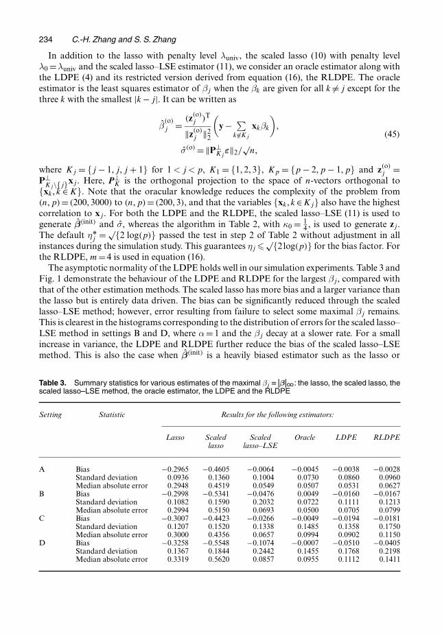
The asymptotic normality of the LDPE holds well in our simulation experiments. Table 3 andFig. 1 demonstrate the behaviour of the LDPE and RLDPE for the largest βj, compared withthat of the other estimation methods. The scaled lasso has more bias and a larger variance thanthe lasso but is entirely data driven. The bias can be significantly reduced through the scaledlasso–LSE method; however, error resulting from failure to select some maximal βj remains.This is clearest in the histograms corresponding to the distribution of errors for the scaled lasso–LSE method in settings B and D, where α= 1 and the βj decay at a slower rate. For a smallincrease in variance, the LDPE and RLDPE further reduce the bias of the scaled lasso–LSEmethod. This is also the case when β.init/ is a heavily biased estimator such as the lasso or
Table 3. Summary statistics for various estimates of the maximal βj Djβj1: the lasso, the scaled lasso, thescaled lasso–LSE method, the oracle estimator, the LDPE and the RLDPE
Setting Statistic Results for the following estimators:
Lasso Scaled Scaled Oracle LDPE RLDPElasso lasso–LSE
A Bias −0.2965 −0.4605 −0.0064 −0.0045 −0.0038 −0.0028Standard deviation 0.0936 0.1360 0.1004 0.0730 0.0860 0.0960Median absolute error 0.2948 0.4519 0.0549 0.0507 0.0531 0.0627
B Bias −0.2998 −0.5341 −0.0476 0.0049 −0.0160 −0.0167Standard deviation 0.1082 0.1590 0.2032 0.0722 0.1111 0.1213Median absolute error 0.2994 0.5150 0.0693 0.0500 0.0705 0.0799
C Bias −0.3007 −0.4423 −0.0266 −0.0049 −0.0194 −0.0181Standard deviation 0.1207 0.1520 0.1338 0.1485 0.1358 0.1750Median absolute error 0.3000 0.4356 0.0657 0.0994 0.0902 0.1150
D Bias −0.3258 −0.5548 −0.1074 −0.0007 −0.0510 −0.0405Standard deviation 0.1367 0.1844 0.2442 0.1455 0.1768 0.2198Median absolute error 0.3319 0.5620 0.0857 0.0955 0.1112 0.1411
Confidence Intervals for Low Dimensional Parameters 235
(a) (b) (c) (d)
(e) (f) (g) (h)
(i) (j) (k) (l)
(m) (n) (o) (p)
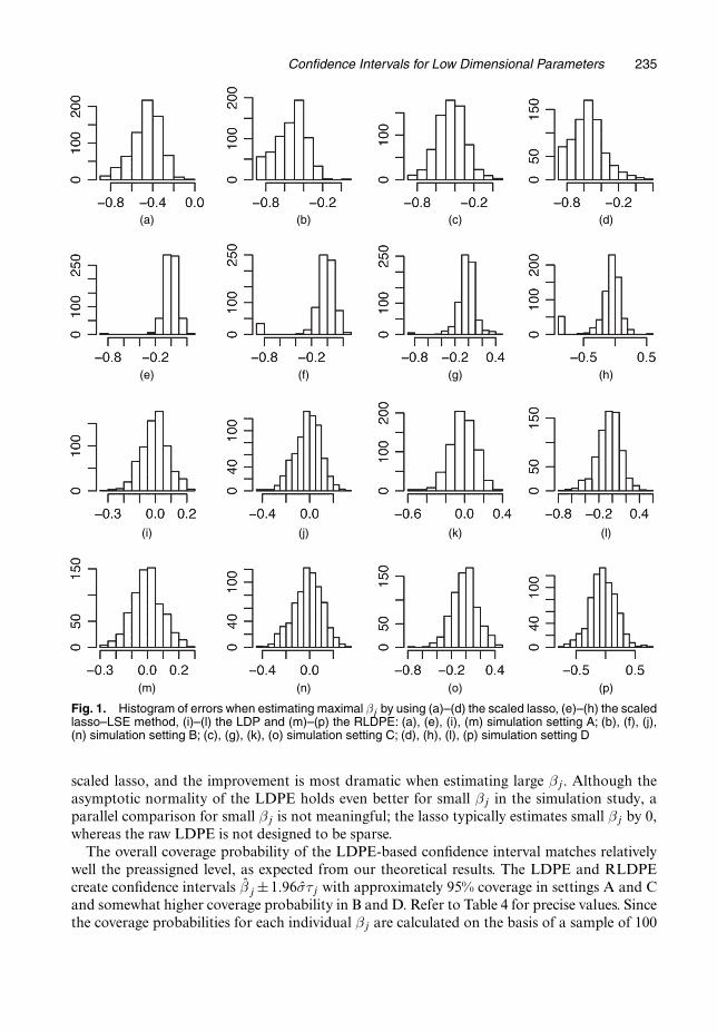
Fig. 1. Histogram of errors when estimating maximal βj by using (a)–(d) the scaled lasso, (e)–(h) the scaledlasso–LSE method, (i)–(l) the LDP and (m)–(p) the RLDPE: (a), (e), (i), (m) simulation setting A; (b), (f), (j),(n) simulation setting B; (c), (g), (k), (o) simulation setting C; (d), (h), (l), (p) simulation setting D
scaled lasso, and the improvement is most dramatic when estimating large βj. Although theasymptotic normality of the LDPE holds even better for small βj in the simulation study, aparallel comparison for small βj is not meaningful; the lasso typically estimates small βj by 0,whereas the raw LDPE is not designed to be sparse.
The overall coverage probability of the LDPE-based confidence interval matches relativelywell the preassigned level, as expected from our theoretical results. The LDPE and RLDPEcreate confidence intervals βj±1:96στj with approximately 95% coverage in settings A and Cand somewhat higher coverage probability in B and D. Refer to Table 4 for precise values. Sincethe coverage probabilities for each individual βj are calculated on the basis of a sample of 100
236 C.-H. Zhang and S. S. Zhang
(a) (b) (c) (d)
(e) (f) (g) (h)
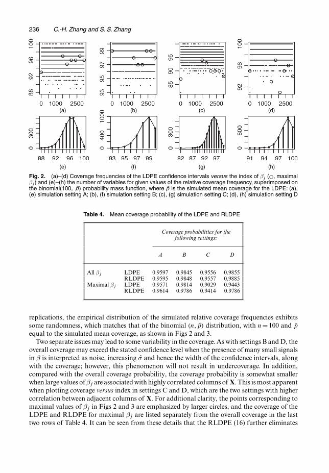
Fig. 2. (a)–(d) Coverage frequencies of the LDPE confidence intervals versus the index of βj (�, maximalβj ) and (e)–(h) the number of variables for given values of the relative coverage frequency, superimposed onthe binomial(100, p) probability mass function, where p is the simulated mean coverage for the LDPE: (a),(e) simulation setting A; (b), (f) simulation setting B; (c), (g) simulation setting C; (d), (h) simulation setting D
Table 4. Mean coverage probability of the LDPE and RLDPE
Coverage probabilities for thefollowing settings:
A B C D
All βj LDPE 0.9597 0.9845 0.9556 0.9855RLDPE 0.9595 0.9848 0.9557 0.9885
Maximal βj LDPE 0.9571 0.9814 0.9029 0.9443RLDPE 0.9614 0.9786 0.9414 0.9786
replications, the empirical distribution of the simulated relative coverage frequencies exhibitssome randomness, which matches that of the binomial .n, p/ distribution, with n= 100 and p
equal to the simulated mean coverage, as shown in Figs 2 and 3.Two separate issues may lead to some variability in the coverage. As with settings B and D, the
overall coverage may exceed the stated confidence level when the presence of many small signalsin β is interpreted as noise, increasing σ and hence the width of the confidence intervals, alongwith the coverage; however, this phenomenon will not result in undercoverage. In addition,compared with the overall coverage probability, the coverage probability is somewhat smallerwhen large values of βj are associated with highly correlated columns of X. This is most apparentwhen plotting coverage versus index in settings C and D, which are the two settings with highercorrelation between adjacent columns of X. For additional clarity, the points corresponding tomaximal values of βj in Figs 2 and 3 are emphasized by larger circles, and the coverage of theLDPE and RLDPE for maximal βj are listed separately from the overall coverage in the lasttwo rows of Table 4. It can be seen from these details that the RLDPE (16) further eliminates
Confidence Intervals for Low Dimensional Parameters 237
(a) (b) (c) (d)
(e) (f) (g) (h)
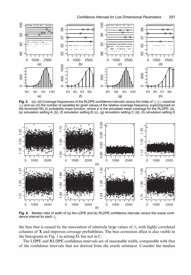
Fig. 3. (a)–(d) Coverage frequencies of the RLDPE confidence intervals versus the index of βj (�, maximalβj / and (e)–(h) the number of variables for given values of the relative coverage frequency, superimposed onthe binomial(100, p) probability mass function, where p is the simulated mean coverage for the RLDPE: (a),(e) simulation setting A; (b), (f) simulation setting B; (c), (g) simulation setting C; (d), (h) simulation setting D
(a)
(b)
Fig. 4. Median ratio of width of (a) the LDPE and (b) RLDPE confidence intervals versus the oracle confi-dence interval for each βj
the bias that is caused by the association of relatively large values of βj with highly correlatedcolumns of X and improves coverage probabilities. The bias correction effect is also visible inthe histograms in Fig. 1 in setting D, but not in C.
The LDPE and RLDPE confidence intervals are of reasonable width, comparable with thatof the confidence intervals that are derived from the oracle estimator. Consider the median
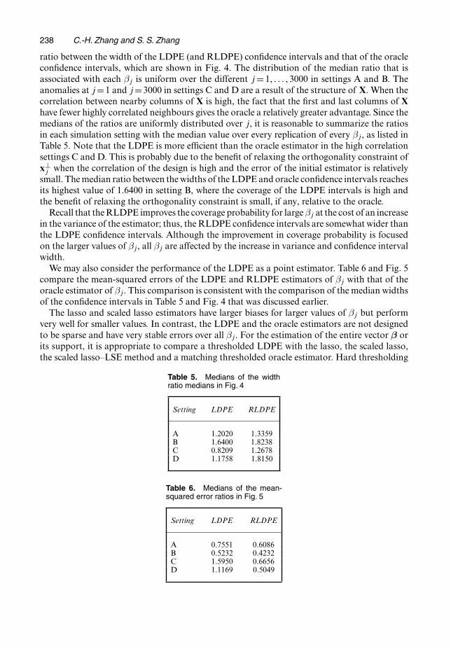
238 C.-H. Zhang and S. S. Zhang
ratio between the width of the LDPE (and RLDPE) confidence intervals and that of the oracleconfidence intervals, which are shown in Fig. 4. The distribution of the median ratio that isassociated with each βj is uniform over the different j= 1, : : : , 3000 in settings A and B. Theanomalies at j=1 and j=3000 in settings C and D are a result of the structure of X. When thecorrelation between nearby columns of X is high, the fact that the first and last columns of Xhave fewer highly correlated neighbours gives the oracle a relatively greater advantage. Since themedians of the ratios are uniformly distributed over j, it is reasonable to summarize the ratiosin each simulation setting with the median value over every replication of every βj, as listed inTable 5. Note that the LDPE is more efficient than the oracle estimator in the high correlationsettings C and D. This is probably due to the benefit of relaxing the orthogonality constraint ofx⊥j when the correlation of the design is high and the error of the initial estimator is relativelysmall. The median ratio between the widths of the LDPE and oracle confidence intervals reachesits highest value of 1.6400 in setting B, where the coverage of the LDPE intervals is high andthe benefit of relaxing the orthogonality constraint is small, if any, relative to the oracle.
Recall that the RLDPE improves the coverage probability for large βj at the cost of an increasein the variance of the estimator; thus, the RLDPE confidence intervals are somewhat wider thanthe LDPE confidence intervals. Although the improvement in coverage probability is focusedon the larger values of βj, all βj are affected by the increase in variance and confidence intervalwidth.
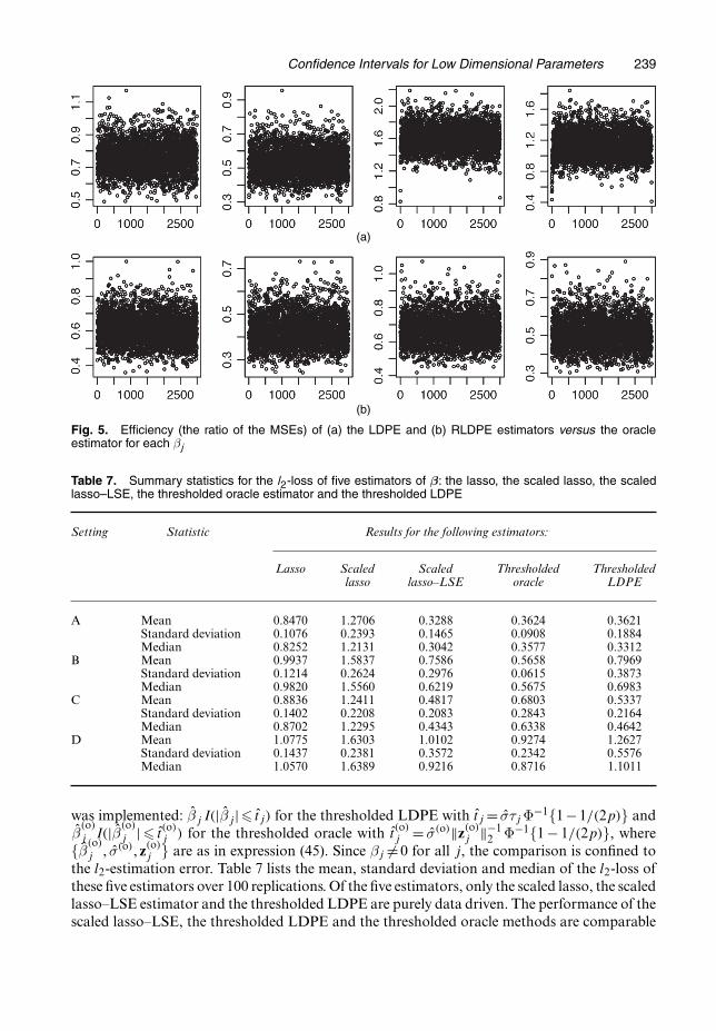
We may also consider the performance of the LDPE as a point estimator. Table 6 and Fig. 5compare the mean-squared errors of the LDPE and RLDPE estimators of βj with that of theoracle estimator of βj. This comparison is consistent with the comparison of the median widthsof the confidence intervals in Table 5 and Fig. 4 that was discussed earlier.
The lasso and scaled lasso estimators have larger biases for larger values of βj but performvery well for smaller values. In contrast, the LDPE and the oracle estimators are not designedto be sparse and have very stable errors over all βj. For the estimation of the entire vector β orits support, it is appropriate to compare a thresholded LDPE with the lasso, the scaled lasso,the scaled lasso–LSE method and a matching thresholded oracle estimator. Hard thresholding
Table 5. Medians of the widthratio medians in Fig. 4
Setting LDPE RLDPE
A 1.2020 1.3359B 1.6400 1.8238C 0.8209 1.2678D 1.1758 1.8150
Table 6. Medians of the mean-squared error ratios in Fig. 5
Setting LDPE RLDPE
A 0.7551 0.6086B 0.5232 0.4232C 1.5950 0.6656D 1.1169 0.5049
Confidence Intervals for Low Dimensional Parameters 239
(a)
(b)
Fig. 5. Efficiency (the ratio of the MSEs) of (a) the LDPE and (b) RLDPE estimators versus the oracleestimator for each βj
Table 7. Summary statistics for the l2-loss of five estimators of β: the lasso, the scaled lasso, the scaledlasso–LSE, the thresholded oracle estimator and the thresholded LDPE
Setting Statistic Results for the following estimators:
Lasso Scaled Scaled Thresholded Thresholdedlasso lasso–LSE oracle LDPE
A Mean 0.8470 1.2706 0.3288 0.3624 0.3621Standard deviation 0.1076 0.2393 0.1465 0.0908 0.1884Median 0.8252 1.2131 0.3042 0.3577 0.3312
B Mean 0.9937 1.5837 0.7586 0.5658 0.7969Standard deviation 0.1214 0.2624 0.2976 0.0615 0.3873Median 0.9820 1.5560 0.6219 0.5675 0.6983
C Mean 0.8836 1.2411 0.4817 0.6803 0.5337Standard deviation 0.1402 0.2208 0.2083 0.2843 0.2164Median 0.8702 1.2295 0.4343 0.6338 0.4642
D Mean 1.0775 1.6303 1.0102 0.9274 1.2627Standard deviation 0.1437 0.2381 0.3572 0.2342 0.5576Median 1.0570 1.6389 0.9216 0.8716 1.1011
was implemented: βj I.|βj|� tj/ for the thresholded LDPE with tj= στj Φ−1{1−1=.2p/} andβ
.o/
j I.|β.o/
j |� t.o/j / for the thresholded oracle with t
.o/j = σ.o/‖z.o/
j ‖−12 Φ−1{1− 1=.2p/}, where
{β.o/
j , σ.o/, z.o/j } are as in expression (45). Since βj = 0 for all j, the comparison is confined to
the l2-estimation error. Table 7 lists the mean, standard deviation and median of the l2-loss ofthese five estimators over 100 replications. Of the five estimators, only the scaled lasso, the scaledlasso–LSE estimator and the thresholded LDPE are purely data driven. The performance of thescaled lasso–LSE, the thresholded LDPE and the thresholded oracle methods are comparable

240 C.-H. Zhang and S. S. Zhang
and they always outperform the scaled lasso. They also outperform the lasso in cases A, B andC. In the hardest case, D, which has both a high correlation between adjacent columns of X anda slower decay in βj, the thresholded oracle slightly outperforms the lasso and the lasso slightlyoutperforms the scaled lasso–LSE and thresholded LDPE methods. Generally, the l2-loss of thethresholded LDPE remains slightly above that of the scaled lasso–LSE method, which improveson the scaled lasso by reducing its bias. Note that our goal is not to find a better estimator for theentire vector β since quite a few versions of the estimation optimality of regularized estimatorshave already been established. What we demonstrate here is that the cost of removing bias withthe LDPE, and thus giving up shrinkage, is small.
5. Discussion
We have developed the LDPE method of constructing β1, : : : , βp for the individual regres-sion coefficients and estimators for their finite dimensional covariance structure. Under properconditions on X and β, we have proved the asymptotic unbiasedness and normality of finitedimensional distribution functions of these estimators and the consistency of their estimatedcovariances. Thus, the LDPE yields an approximate Gaussian sequence as the raw LDPE inexpression (25), which allows us to assess the level of significance of each unknown coefficient βj
without the uniform signal strength assumption (26). The method proposed applies to makinginference about a preconceived low dimensional parameter, which is an interesting practicalproblem and a primary goal of this paper. It also applies to making inference about all regres-sion coefficients via simultaneous interval estimation and the correct selection of large and zerocoefficients in the presence of many small coefficients.
The raw LDPE is not sparse, but it can be thresholded to take advantage of the sparsity ofβ, and the sampling distribution of the thresholded LDPE can still be bounded on the basis ofthe approximate distribution of the raw LDPE. A thresholded LDPE is proven to attain l2-rateoptimality for the estimation of an entire sparse β.
The focus of this paper is interval estimation and hypothesis testing without the uniform signalstrength condition. Another important problem is prediction. Since prediction at a design pointa is equivalent to the estimation of the ‘contrast’ aTβ, with possibly large ‖a‖0, the implicationof the LDPE for prediction is an interesting future research direction.
The proposed LDP approach is closely related to semiparametric inference. This connectionwas discussed in Zhang (2011) along with a definition of the minimum Fisher information anda rationale for the asymptotic efficiency of an LDPE in a general setting.
We use the lasso to provide a relaxation of the projection of xj to x⊥j . This choice is primarilydue to our familiarity with the computation of the lasso and the readily available scaled lassomethod of choosing a penalty level. We have also considered some other methods of relaxingthe projection. A particularly interesting method is the following constrained minimization ofthe variance of the noise term in equation (5):
zj=argminz
{‖z‖22 : |zTj xj|=n, max
k =j|zT
j xk=n|�λ′j}: .46/
Similarly to the lasso in equation (9), equation (46) can be solved via quadratic programming;specifically, one may take the minimizer between the solutions involving the two linear con-straints zT
j xj=±n. The lasso solution (9) is feasible in equation (46) with λjn=|zTj xj|=λ′j.
Acknowledgements
The authors thank a referee and the Associate Editor for their careful reading of the manuscript
Confidence Intervals for Low Dimensional Parameters 241
and for suggestions leading to several improvements. The research of the first author is partiallysupported by National Science Foundation grants DMS 0906420, DMS 1106753 and DMS1209014, and National Security Agency grant H98230-11-1-0205.
References
Antoniadis, A. (2010) Comments on: l1-penalization for mixture regression models. Test, 19, 257–258.Belloni, A., Chernozhukov, V. and Wang, L. (2011) Square-root Lasso: pivotal recovery of sparse signals via conic
programming. Biometrika, 98, 791–806.Berk, R., Brown, L. B. and Zhao, L. (2010) Statistical inference after model selection. J. Quant. Crimin., 26,
217–236.Bickel, P. J. and Levina, E. (2008) Regularized estimation of large covariance matrices. Ann. Statist., 36, 199–
227.Bickel, P., Ritov, Y. and Tsybakov, A. (2009) Simultaneous analysis of Lasso and Dantzig selector. Ann. Statist.,
37, 1705–1732.Buhlmann, P. and van de Geer, S. (2011) Statistics for High-dimensional Data: Methods, Theory and Applications.
New York: Springer.Candes, E. J. and Tao, T. (2005) Decoding by linear programming. IEEE Trans. Inform. Theor., 51, 4203–4215.Candes, E. and Tao, T. (2007) The dantzig selector: statistical estimation when p is much larger than n (with
discussion). Ann. Statist., 35, 2313–2404.Chen, S. S., Donoho, D. L. and Saunders, M. A. (2001) Atomic decomposition by basis pursuit. SIAM Rev., 43,
129–159.Davidson, K. and Szarek, S. (2001) Local operator theory, random matrices and Banach spaces. In Handbook on
the Geometry of Banach Spaces, vol. 1 (eds W. B. Johnson and J. Lindenstrauss). Amsterdam: North-Holland.Donoho, D. L. and Johnstone, I. (1994) Minimax risk over lp-balls for lq-error. Probab. Theor. Reltd Flds, 99,
277–303.Fan, J. and Li, R. (2001) Variable selection via nonconcave penalized likelihood and its oracle properties. J. Am.
Statist. Ass., 96, 1348–1360.Fan, J. and Lv, J. (2008) Sure independence screening for ultrahigh dimensional feature space (with discussion).
J. R. Statist. Soc. B, 70, 849–911.Fan, J. and Lv, J. (2010) A selective overview of variable selection in high dimensional feature space. Statist. Sin.,
20, 101–148.Fan, J. and Peng, H. (2004) On non-concave penalized likelihood with diverging number of parameters. Ann.
Statist., 32, 928–961.Fano, R. (1961) Transmission of Information; a Statistical Theory of Communications. Cambridge: Massachusetts
Institute of Technology Press.Frank, I. E. and Friedman, J. H. (1993) A statistical view of some chemometrics regression tools (with discussion).
Technometrics, 35, 109–148.van de Geer, S. and Buhlmann, P. (2009) On the conditions used to prove oracle results for the Lasso. Electron.
J. Statist., 3, 1360–1392.Greenshtein, E. (2006) Best subset selection, persistence in high-dimensional statistical learning and optimization
under l1 constraint. Ann. Statist., 34, 2367–2386.Greenshtein, E. and Ritov, Y. (2004) Persistence in high-dimensional linear predictor selection and the virtue of
overparametrization. Bernoulli, 10, 971–988.Huang, J., Ma, S. and Zhang, C.-H. (2008) Adaptive Lasso for sparse high-dimensional regression models. Statist.
Sin., 18, 1603–1618.Huang, J. and Zhang, C.-H. (2012) Estimation and selection via absolute penalized convex minimization and its
multistage adaptive applications. J. Mach. Learn. Res., 13, 1809–1834.Kim, Y., Choi, H. and Oh, H.-S. (2008) Smoothly clipped absolute deviation on high dimensions. J. Am. Statist.
Ass., 103, 1665–1673.Koltchinskii, V. (2009) The dantzig selector and sparsity oracle inequalities. Bernoulli, 15, 799–828.Koltchinskii, V., Lounici, K. and Tsybakov, A. B. (2011) Nuclear-norm penalization and optimal rates for noisy
low-rank matrix completion. Ann. Statist., 39, 2302–2329.Laber, E. and Murphy, S. A. (2011) Adaptive confidence intervals for the test error in classification (with discus-
sion). J. Am. Statist. Ass., 106, 904–913.Leeb, H. and Potscher, B. M. (2006) Can one estimate the conditional distribution of post-model-selection es-
timators? Ann. Statist., 34, 2554–2591.Meinshausen, N. and Buhlmann, P. (2006) High-dimensional graphs and variable selection with the Lasso. Ann.
Statist., 34, 1436–1462.Meinshausen, N. and Buhlmann, P. (2010) Stability selection (with discussion). J. R. Statist. Soc. B, 72, 417–473.Meinshausen, N. and Yu, B. (2009) Lasso-type recovery of sparse representations for high-dimensional data. Ann.
Statist., 37, 246–270.

242 C.-H. Zhang and S. S. Zhang
Stadler, N., Buhlmann, P. and van de Geer, S. (2010) l1-penalization for mixture regression models (with discus-sion). Test, 19, 209–285.
Sun, T. and Zhang, C.-H. (2010) Comments on: l1-penalization for mixture regression models. Test, 19, 270–275.Sun, T. and Zhang, C.-H. (2012) Scaled sparse linear regression. Biometrika, 99, 879–898.Tibshirani, R. (1996) Regression shrinkage and selection via the lasso. J. R. Statist. Soc. B, 58, 267–288.Tropp, J. A. (2006) Just relax: convex programming methods for identifying sparse signals in noise. IEEE Trans.
Inform. Theor., 52, 1030–1051.Wainwright, M. J. (2009a) Sharp thresholds for noisy and high-dimensional recovery of sparsity using l1-
constrained quadratic programming (Lasso). IEEE Trans. Inform. Theor., 55, 2183–2202.Wainwright, M. J. (2009b) Information-theoretic limitations on sparsity recovery in the high-dimensional and
noisy setting. IEEE Trans. Inform. Theor., 55, 5728–5741.Ye, F. and Zhang, C.-H. (2010) Rate minimaxity of the Lasso and Dantzig selector for the lq loss in lr balls. J.
Mach. Learn. Res., 11, 3481–3502.Zhang, C.-H. (2010) Nearly unbiased variable selection under minimax concave penalty. Ann. Statist., 38, 894–942.Zhang, C.-H. (2011) Statistical inference for high-dimensional data. In Very High Dimensional Semiparametric
Models, Report No. 48/2011, pp. 28–31. Mathematisches Forschungsinstitut Oberwolfach.Zhang, C.-H. and Huang, J. (2008) The sparsity and bias of the Lasso selection in high-dimensional linear
regression. Ann. Statist., 36, 1567–1594.Zhang, C.-H. and Zhang, S. S. (2011) Confidence intervals for low-dimensional parameters in high-dimensional
linear models. Preprint arXiv:1110.2563.Zhang, C.-H. and Zhang, T. (2012) A general theory of concave regularization for high dimensional sparse
estimation problems. Statist. Sci., 27, 576–593.Zhang, T. (2009) Some sharp performance bounds for least squares regression with L1 regularization. Ann. Statist.,
37, no. 5A, 2109–2144.Zhang, T. (2011a) Adaptive forward-backward greedy algorithm for learning sparse representations. IEEE Trans.
Inform. Theor., 57, 4689–4708.Zhang, T. (2011b) Multi-stage convex relaxation for feature selection. Preprint arXiv:1106.0565.Zhao, P. and Yu, B. (2006) On model selection consistency of Lasso. J. Mach. Learn. Res., 7, 2541–2567.Zou, H. (2006) The adaptive Lasso and its oracle properties. J. Am. Statist. Ass., 101, 1418–1429.Zou, H. and Li, R. (2008) One-step sparse estimates in nonconcave penalized likelihood models. Ann. Statist., 36,
1509–1533.
Supporting informationAdditional ‘supporting information’ may be found in the on-line version of this article:
‘Supplement material for Confidence intervals for low-dimensional parameters in high-dimensional linear models’.