Confidence Interval Module - faculty.nps.edufaculty.nps.edu/rdfricke/OA3102/Interval Estimation -...
62
Revision: 1-12 1 Module 5: Interval Estimation Statistics (OA3102) Professor Ron Fricker Naval Postgraduate School Monterey, California Reading assignment: WM&S chapter 8.5-8.9
Transcript of Confidence Interval Module - faculty.nps.edufaculty.nps.edu/rdfricke/OA3102/Interval Estimation -...
Revision: 1-12 1
Module 5: Interval Estimation Statistics (OA3102)
Professor Ron Fricker Naval Postgraduate School
Monterey, California
Reading assignment:
WM&S chapter 8.5-8.9
Revision: 1-12 2
Goals for this Module
• Interval estimation – i.e., confidence intervals
– Terminology
– Pivotal method for creating confidence intervals
• Types of intervals
– Large-sample confidence intervals
– One-sided vs. two-sided intervals
– Small-sample confidence intervals for the mean,
differences in two means
– Confidence interval for the variance
• Sample size calculations
Interval Estimation
• Instead of estimating a parameter with a
single number, estimate it with an interval
• Ideally, interval will have two properties:
– It will contain the target parameter q
– It will be relatively narrow
• But, as we will see, since interval endpoints
are a function of the data,
– They will be variable
– So we cannot be sure q will fall in the interval
Revision: 1-12 3
Objective for Interval Estimation
• So, we can’t be sure that the interval
contains q, but we will be able to
calculate the probability the interval
contains q
• Interval estimation objective: Find an
interval estimator capable of generating
narrow intervals with a high probability
of enclosing q
Revision: 1-12 4
Revision: 1-12 5
Why Interval Estimation?
• As before, we want to use a sample to infer
something about a larger population
• However, samples are variable
– We’d get different values with each new sample
– So our point estimates are variable
• Point estimates do not give any information about
how far off we might be (precision)
• Interval estimation helps us do inference in such a
way that:
– We can know how precise our estimates are, and
– We can define the probability we are right
Terminology
• Interval estimators are commonly called
confidence intervals
• Interval endpoints are called the upper
and lower confidence limits
• The probability the interval will enclose
q is called the confidence coefficient or
confidence level – Notation: 1-a or 100(1-a)%
– Usually referred to as “100(1-a)” percent CIs Revision: 1-12 6
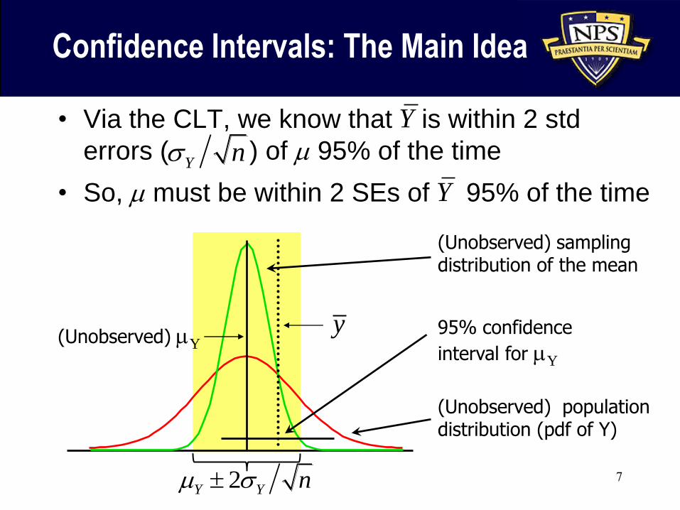
• Via the CLT, we know that is within 2 std
errors ( ) of m 95% of the time
(Unobserved) population distribution (pdf of Y)
(Unobserved) sampling distribution of the mean
(Unobserved) mY
7
Y
Confidence Intervals: The Main Idea
Y n
y
2Y Y nm
95% confidence
interval for mY
• So, m must be within 2 SEs of 95% of the time Y
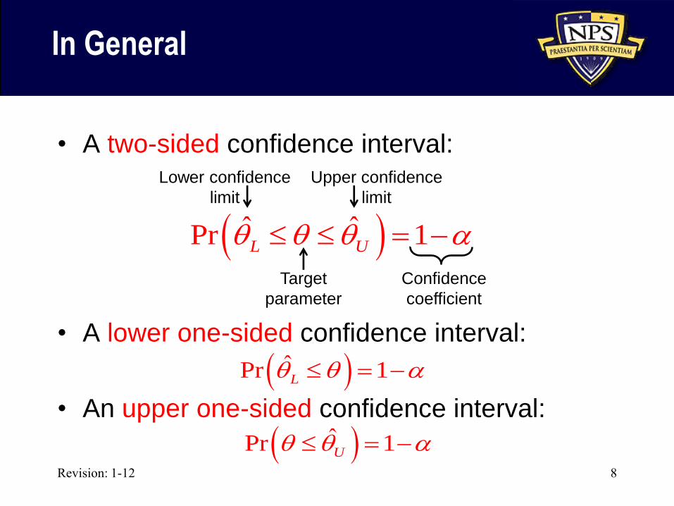
• A two-sided confidence interval:
• A lower one-sided confidence interval:
• An upper one-sided confidence interval:
Upper confidence
limit
In General
Revision: 1-12 8
ˆ ˆPr 1L Uq q q a
Confidence
coefficient
Target
parameter
Lower confidence
limit
ˆPr 1Lq q a
ˆPr 1Uq q a
Revision: 1-12 9
Pivotal Method: A Strategy
for Constructing CIs
• Pivotal method approach
– Find a “pivotal quantity” that has following two
characteristics:
• It is a function of the sample data and q, where
q is the only unknown quantity
• Probability distribution of pivotal quantity does
not depend on q (and you know what it is)
• Now, write down an appropriate probability
statement for the pivotal quantity and then
rearrange terms…
Revision: 1-12 10
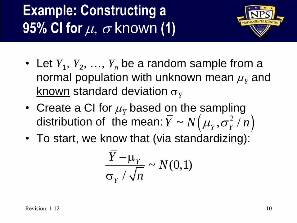
Example: Constructing a
95% CI for m, known (1)
• Let Y1, Y2, …, Yn be a random sample from a
normal population with unknown mean mY and
known standard deviation Y
• Create a CI for mY based on the sampling
distribution of the mean:
• To start, we know that (via standardizing):
~ (0,1)
/
Y
Y
YN
n
m
2~ , /Y YY N nm
Revision: 1-12 11
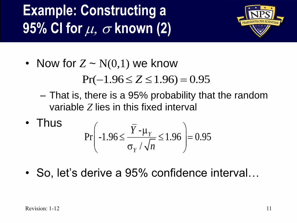
Example: Constructing a
95% CI for m, known (2)
• Now for Z ~ N(0,1) we know
– That is, there is a 95% probability that the random
variable Z lies in this fixed interval
• Thus
• So, let’s derive a 95% confidence interval…
Pr( 1.96 1.96) 0.95Z
-Pr -1.96 1.96 0.95
/
Y
Y
Y
n
m
Revision: 1-12 12
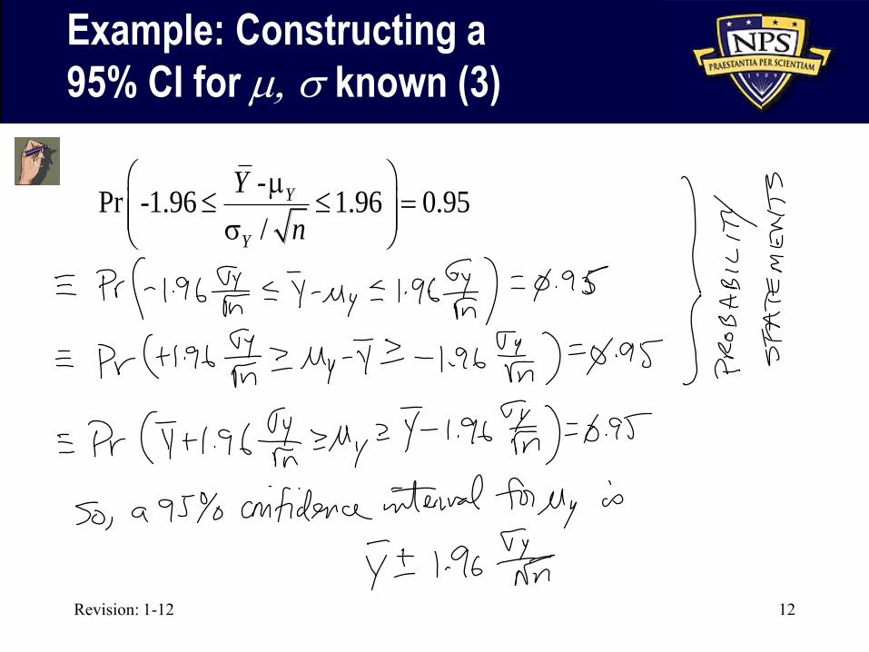
Example: Constructing a
95% CI for m, known (3)
-Pr -1.96 1.96 0.95
/
Y
Y
Y
n
m
Revision: 1-12 13
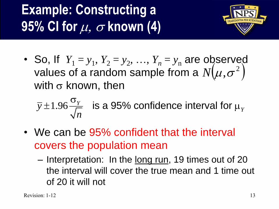
Example: Constructing a
95% CI for m, known (4)
• So, If Y1 = y1, Y2 = y2, …, Yn = yn are observed
values of a random sample from a
with known, then
• We can be 95% confident that the interval
covers the population mean
– Interpretation: In the long run, 19 times out of 20
the interval will cover the true mean and 1 time out
of 20 it will not
1.96 YYy
n
mis a 95% confidence interval for
2,mN
Revision: 1-12 14
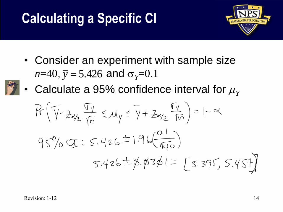
Calculating a Specific CI
• Consider an experiment with sample size
n=40, and Y=0.1
• Calculate a 95% confidence interval for mY
5.426y
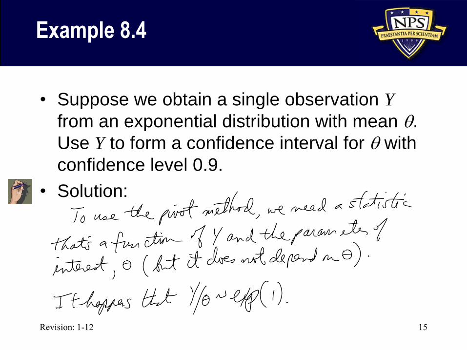
Example 8.4
• Suppose we obtain a single observation Y
from an exponential distribution with mean q.
Use Y to form a confidence interval for q with
confidence level 0.9.
• Solution:
Revision: 1-12 15
Revision: 1-12 16
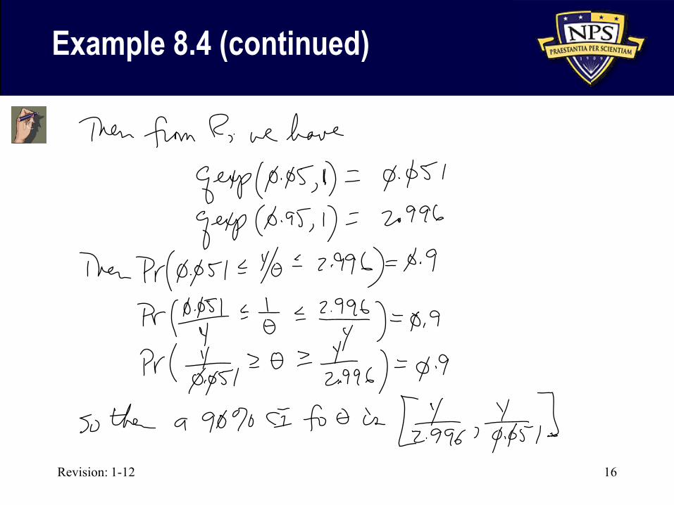
Example 8.4 (continued)
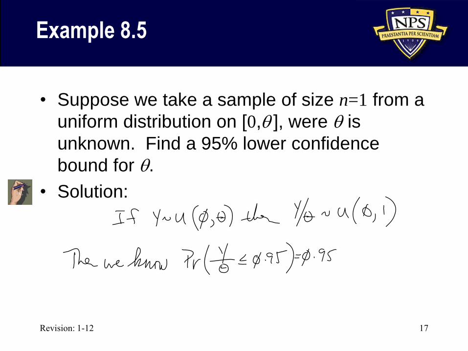
Example 8.5
• Suppose we take a sample of size n=1 from a
uniform distribution on [0,q ], were q is
unknown. Find a 95% lower confidence
bound for q.
• Solution:
Revision: 1-12 17
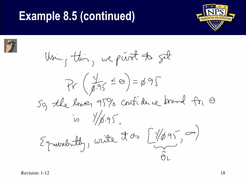
Revision: 1-12 18
Example 8.5 (continued)
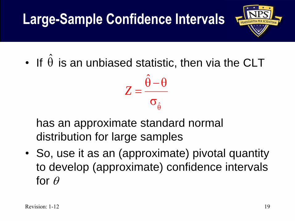
Large-Sample Confidence Intervals
• If is an unbiased statistic, then via the CLT
has an approximate standard normal
distribution for large samples
• So, use it as an (approximate) pivotal quantity
to develop (approximate) confidence intervals
for q
Revision: 1-12 19
ˆ
ˆZ
q
q q
q̂
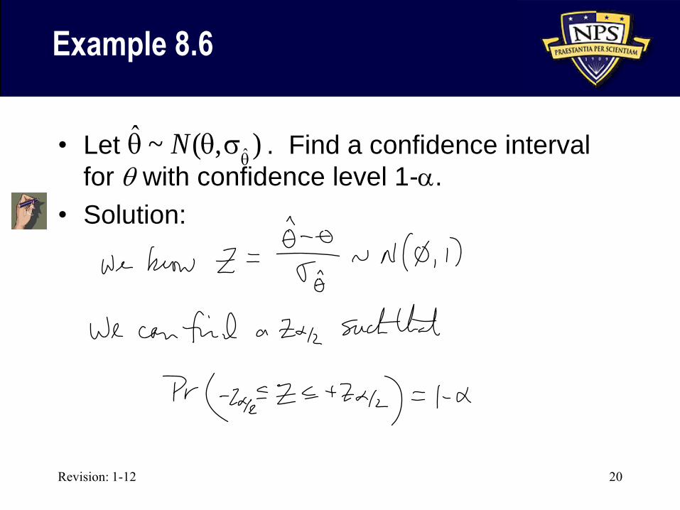
Example 8.6
• Let . Find a confidence interval
for q with confidence level 1-a.
• Solution:
Revision: 1-12 20
ˆˆ ~ ( , )N
qq q
Revision: 1-12 21
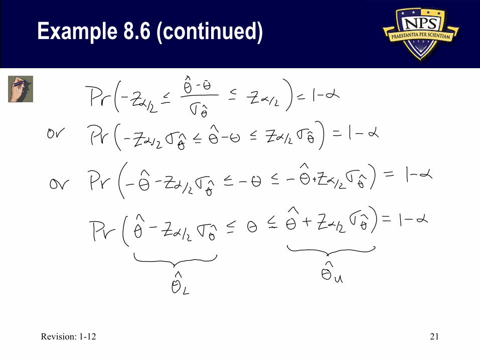
Example 8.6 (continued)
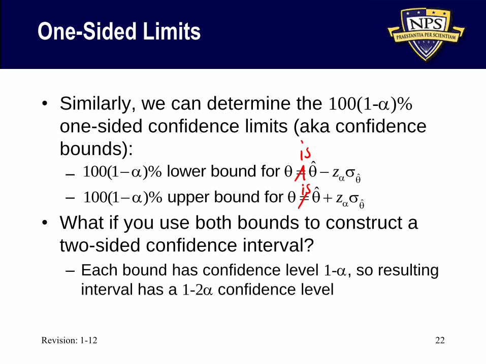
One-Sided Limits
• Similarly, we can determine the 100(1-a)%
one-sided confidence limits (aka confidence
bounds):
–
–
• What if you use both bounds to construct a
two-sided confidence interval?
– Each bound has confidence level 1-a, so resulting
interval has a 1-2a confidence level
Revision: 1-12 22
ˆˆ100(1 )% za q
a q q lower bound for
ˆˆ100(1 )% za q
a q q upper bound for
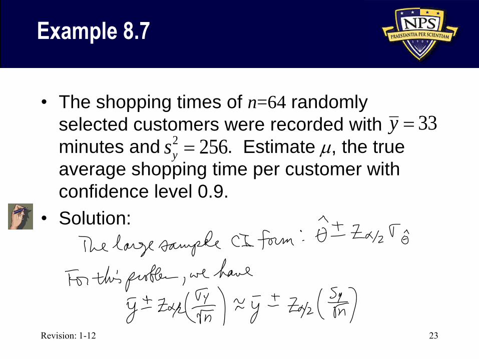
Example 8.7
• The shopping times of n=64 randomly
selected customers were recorded with
minutes and . Estimate m, the true
average shopping time per customer with
confidence level 0.9.
• Solution:
Revision: 1-12 23
33y 2 256ys
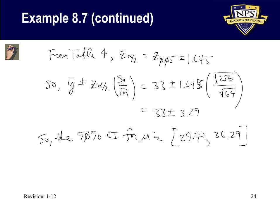
Revision: 1-12 24
Example 8.7 (continued)
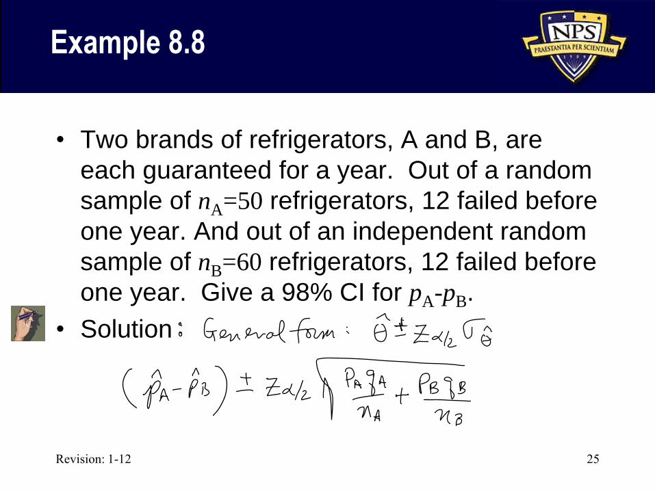
Example 8.8
• Two brands of refrigerators, A and B, are
each guaranteed for a year. Out of a random
sample of nA=50 refrigerators, 12 failed before
one year. And out of an independent random
sample of nB=60 refrigerators, 12 failed before
one year. Give a 98% CI for pA-pB.
• Solution
Revision: 1-12 25
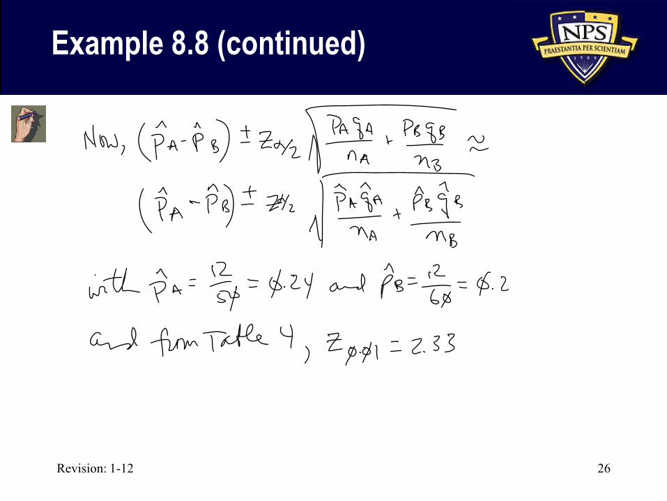
Revision: 1-12 26
Example 8.8 (continued)
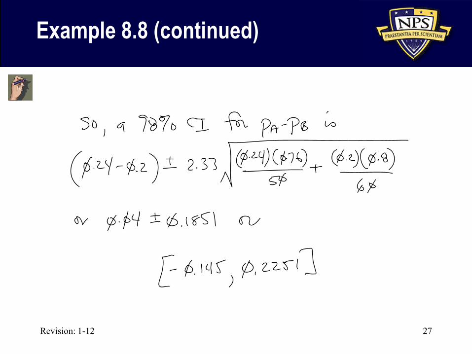
Revision: 1-12 27
Example 8.8 (continued)
Revision: 1-12 28
What is a Confidence Interval?
• Before collecting data and calculating it, a confidence
interval is a random interval
– Random because it is a function of a random variable (e.g., )
• The confidence level is the long-run percentage of
intervals that will “cover” the population parameter
– It is not the probability a particular interval contains the
parameter!
• This statement implies that the parameter is random
• After collecting the data and calculating the CI
the interval is fixed
– It then contains the parameter with probability 0 or 1
Y
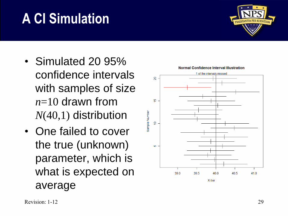
A CI Simulation
Revision: 1-12 29
• Simulated 20 95%
confidence intervals
with samples of size
n=10 drawn from
N(40,1) distribution
• One failed to cover
the true (unknown)
parameter, which is
what is expected on
average
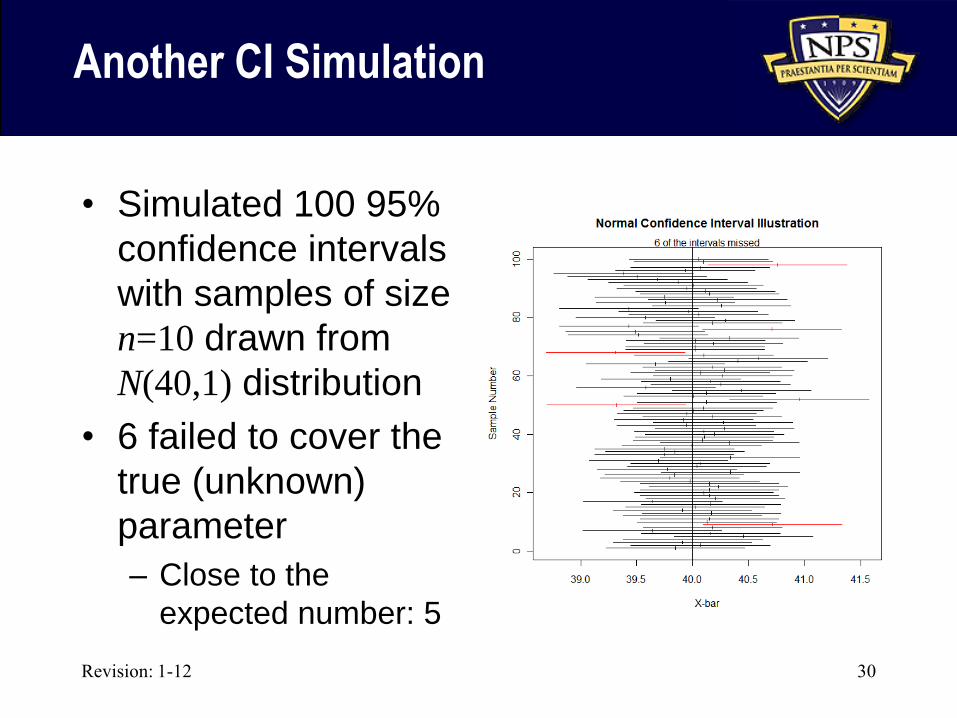
Another CI Simulation
Revision: 1-12 30
• Simulated 100 95%
confidence intervals
with samples of size
n=10 drawn from
N(40,1) distribution
• 6 failed to cover the
true (unknown)
parameter
– Close to the
expected number: 5
Revision: 1-12 31
Illustrating Confidence Intervals
This is a demonstration showing confidence
intervals for a proportion.
Applets created by Prof Gary McClelland, University of Colorado, Boulder
You can access them at
www.thomsonedu.com/statistics/book_content/0495110817_wackerly/applets/seeingstats/index.html
TO DEMO
Revision: 1-12 32
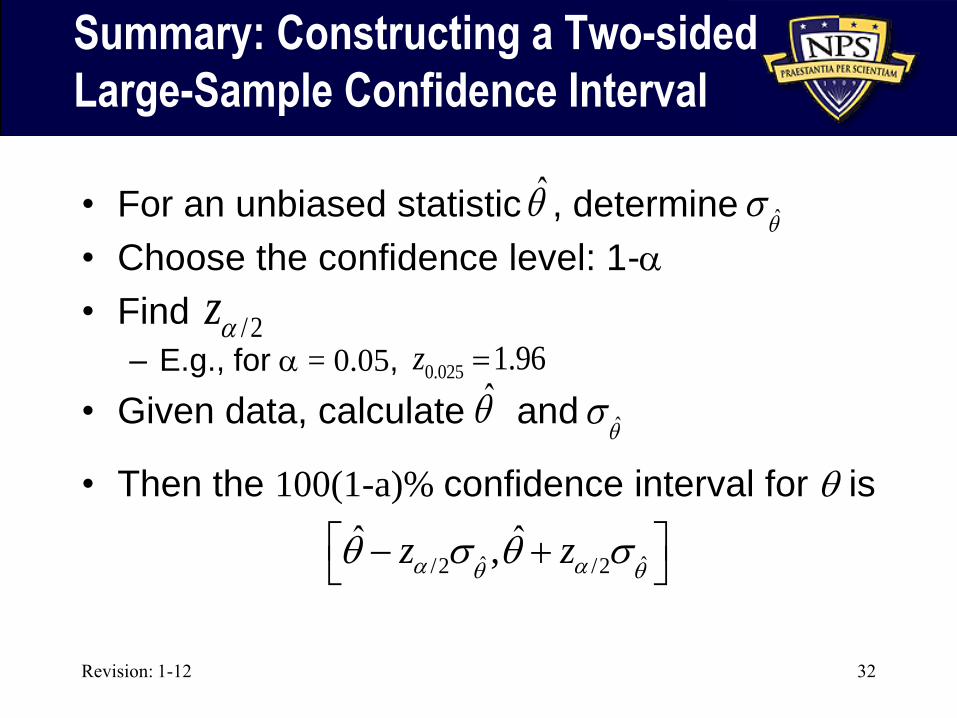
Summary: Constructing a Two-sided
Large-Sample Confidence Interval
• For an unbiased statistic , determine
• Choose the confidence level: 1-a
• Find
– E.g., for a = 0.05,
• Given data, calculate and
• Then the 100(1-a)% confidence interval for q is
ˆ ˆ/2 /2
ˆ ˆ,z za aq qq q
0.025 1.96z /2za
q̂q̂
q̂q̂
Revision: 1-12 33
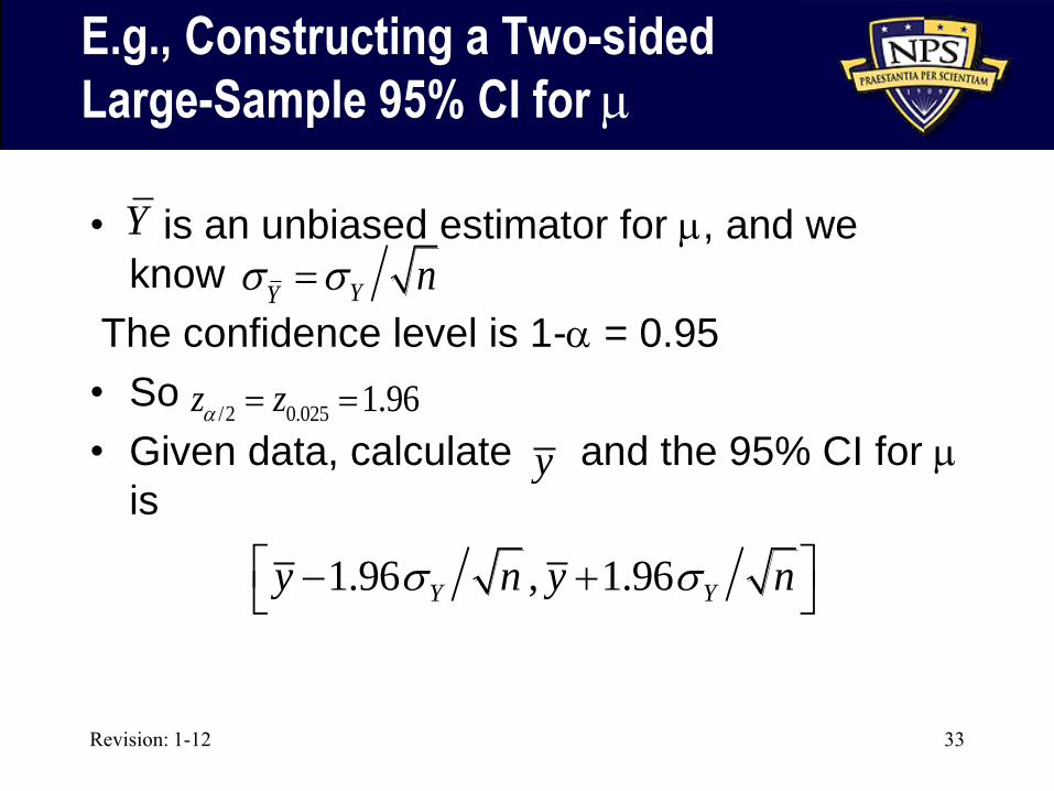
E.g., Constructing a Two-sided
Large-Sample 95% CI for m
• is an unbiased estimator for m, and we
know
The confidence level is 1-a = 0.95
• So
• Given data, calculate and the 95% CI for m
is
Y
/2 0.025 1.96z za
YYn
y
1.96 , 1.96Y Yy n y n
Revision: 1-12 34
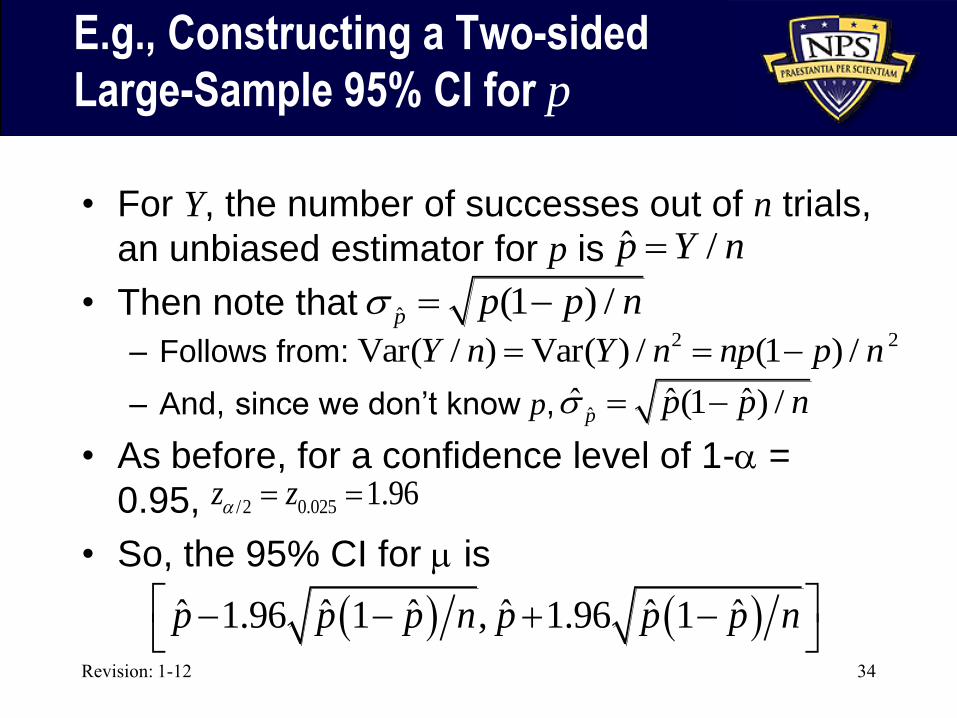
E.g., Constructing a Two-sided
Large-Sample 95% CI for p
• For Y, the number of successes out of n trials,
an unbiased estimator for p is
• Then note that
– Follows from:
– And, since we don’t know p,
• As before, for a confidence level of 1-a =
0.95,
• So, the 95% CI for m is
/2 0.025 1.96z za
ˆ ˆ ˆ ˆ ˆ ˆ1.96 1 , 1.96 1p p p n p p p n
ˆ /p Y n
ˆ (1 ) /p p p n
ˆˆ ˆ ˆ(1 ) /p p p n
2 2Var( / ) Var( ) / (1 ) /Y n Y n np p n
Revision: 1-12 35
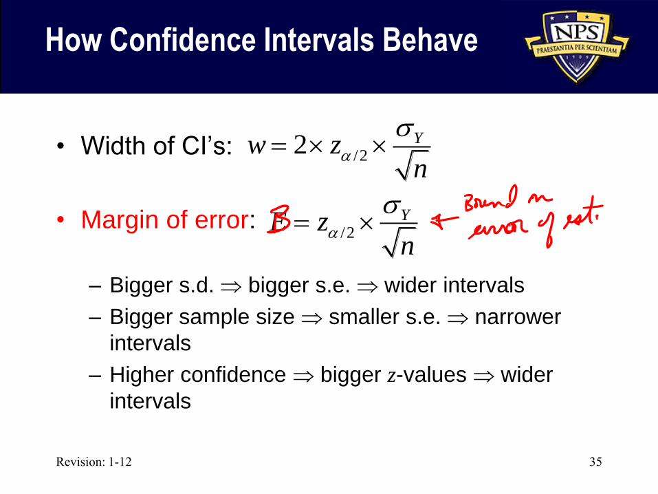
How Confidence Intervals Behave
• Width of CI’s:
• Margin of error:
– Bigger s.d. bigger s.e. wider intervals
– Bigger sample size smaller s.e. narrower
intervals
– Higher confidence bigger z-values wider
intervals
/22 Yw zn
a
/2YE zn
a
Revision: 1-12 36
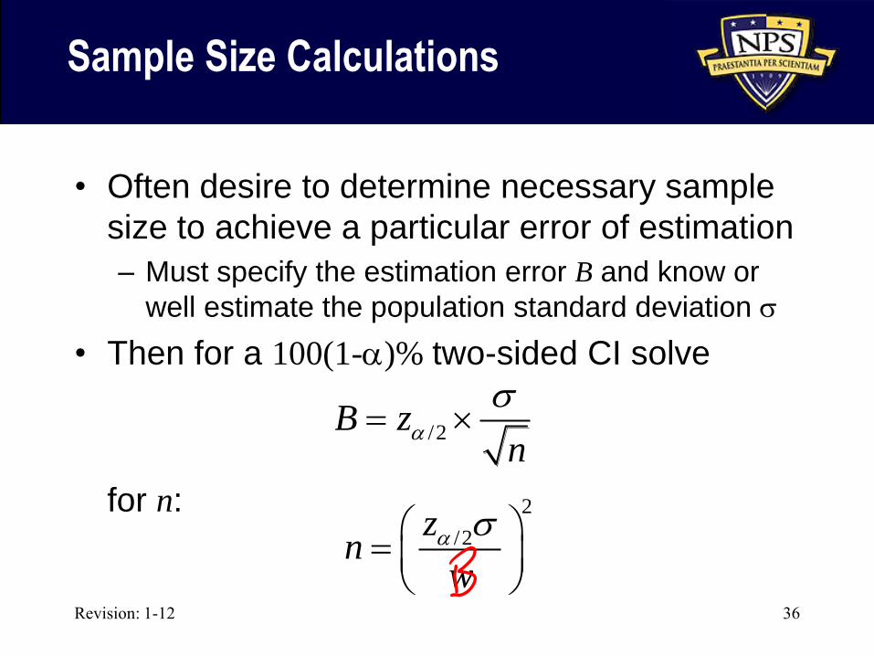
Sample Size Calculations
• Often desire to determine necessary sample
size to achieve a particular error of estimation
– Must specify the estimation error B and know or
well estimate the population standard deviation
• Then for a 100(1-a)% two-sided CI solve
for n:
/2B zn
a
2
/2zn
w
a
Revision: 1-12 37
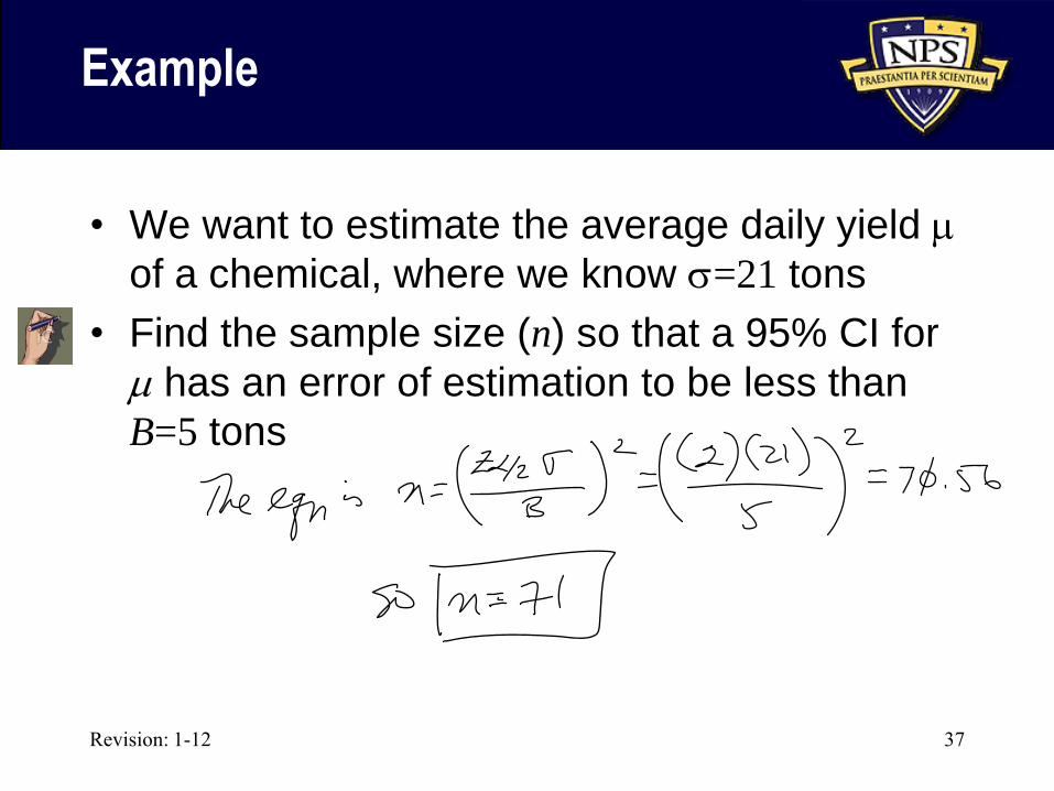
Example
• We want to estimate the average daily yield m
of a chemical, where we know =21 tons
• Find the sample size (n) so that a 95% CI for
m has an error of estimation to be less than
B=5 tons
Revision: 1-12 38
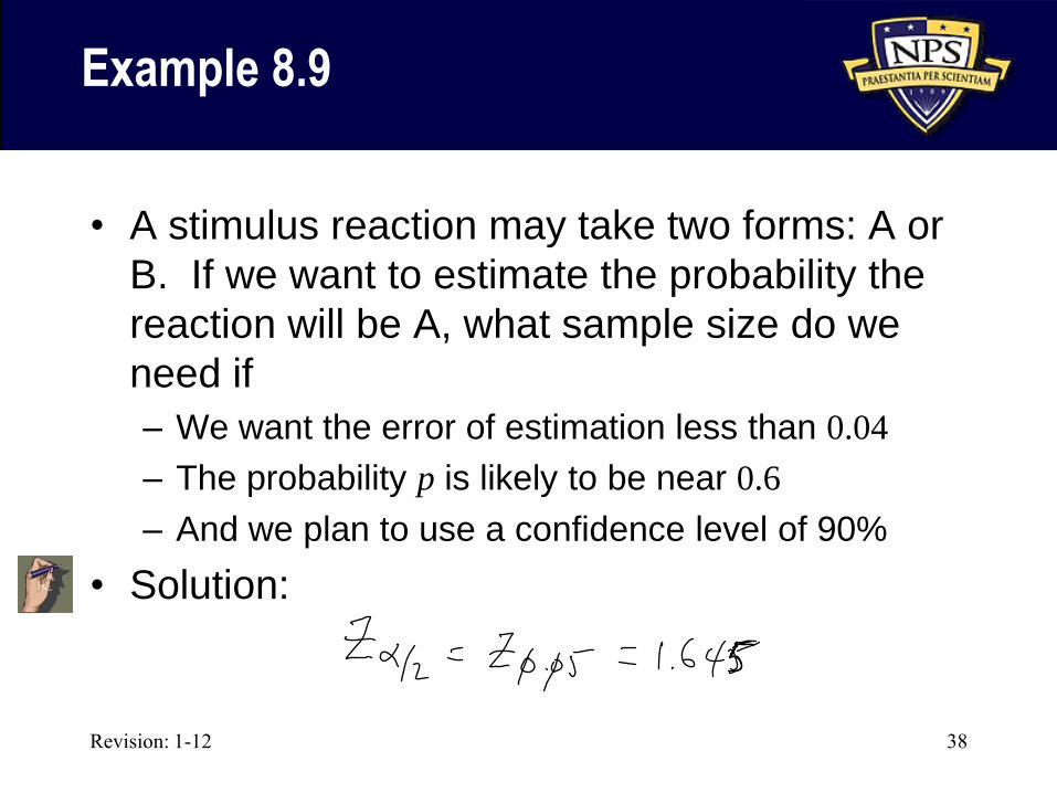
Example 8.9
• A stimulus reaction may take two forms: A or
B. If we want to estimate the probability the
reaction will be A, what sample size do we
need if
– We want the error of estimation less than 0.04
– The probability p is likely to be near 0.6
– And we plan to use a confidence level of 90%
• Solution:
Revision: 1-12 39
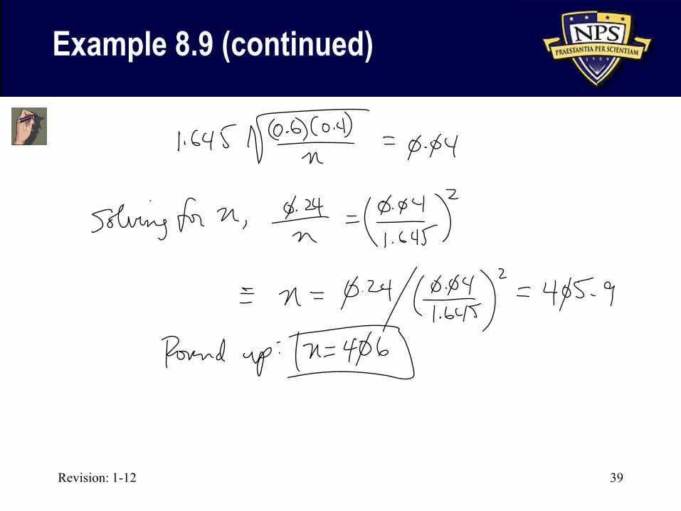
Example 8.9 (continued)
Revision: 1-12 40
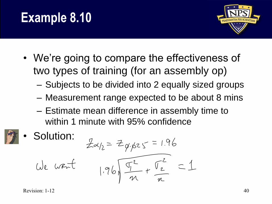
Example 8.10
• We’re going to compare the effectiveness of
two types of training (for an assembly op)
– Subjects to be divided into 2 equally sized groups
– Measurement range expected to be about 8 mins
– Estimate mean difference in assembly time to
within 1 minute with 95% confidence
• Solution:
Revision: 1-12 41
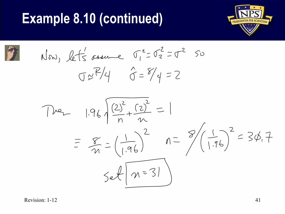
Example 8.10 (continued)
Revision: 1-12 42
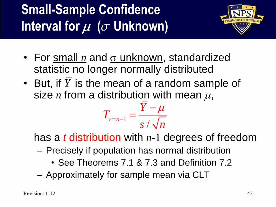
Small-Sample Confidence
Interval for m ( Unknown)
• For small n and unknown, standardized statistic no longer normally distributed
• But, if is the mean of a random sample of size n from a distribution with mean m,
has a t distribution with n-1 degrees of freedom – Precisely if population has normal distribution
• See Theorems 7.1 & 7.3 and Definition 7.2
– Approximately for sample mean via CLT
1/
n
YT
s n
m
Y
Revision: 1-12 43
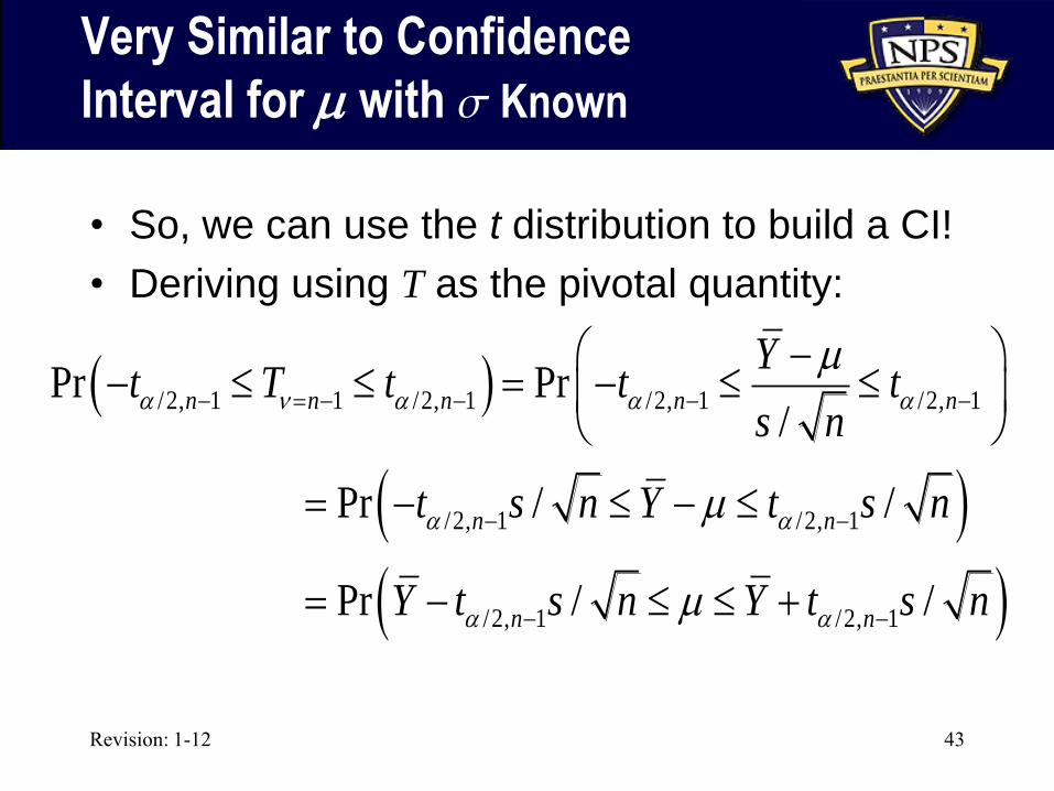
Very Similar to Confidence
Interval for m with Known
• So, we can use the t distribution to build a CI!
• Deriving using T as the pivotal quantity:
/2, 1 1 /2, 1 /2, 1 /2, 1
/2, 1 /2, 1
/2, 1 /2, 1
Pr Pr/
Pr / /
Pr / /
n n n n n
n n
n n
Yt T t t t
s n
t s n Y t s n
Y t s n Y t s n
a a a a
a a
a a
m
m
m
Revision: 1-12 44
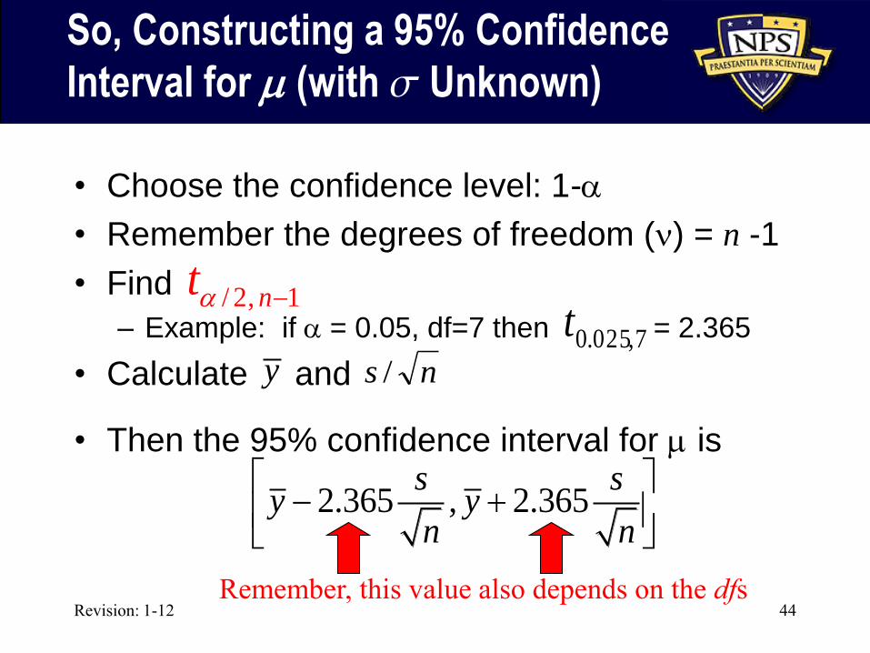
So, Constructing a 95% Confidence
Interval for m (with Unknown)
• Choose the confidence level: 1-a
• Remember the degrees of freedom () = n -1
• Find
– Example: if a = 0.05, df=7 then = 2.365
• Calculate and
• Then the 95% confidence interval for m is
y ns /
2.365 , 2.365s s
y yn n
1,2/ nta
7,025.0t
Remember, this value also depends on the dfs
Revision: 1-12 45
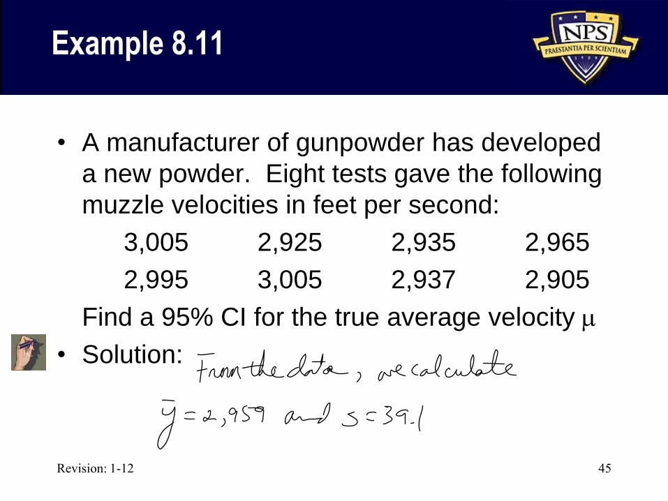
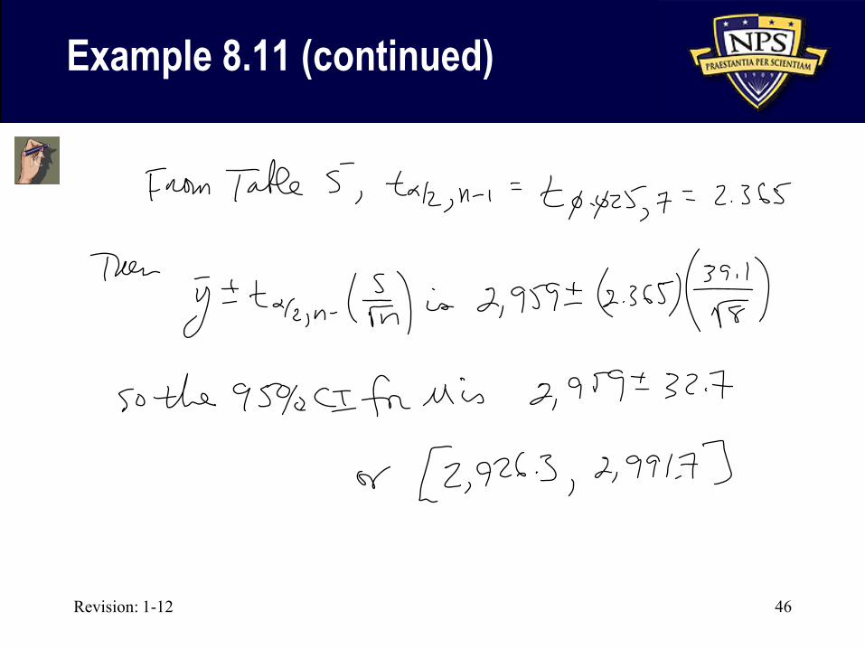
Example 8.11
• A manufacturer of gunpowder has developed
a new powder. Eight tests gave the following
muzzle velocities in feet per second:
3,005 2,925 2,935 2,965
2,995 3,005 2,937 2,905
Find a 95% CI for the true average velocity m
• Solution:
Revision: 1-12 46
Example 8.11 (continued)
Revision: 1-12 47
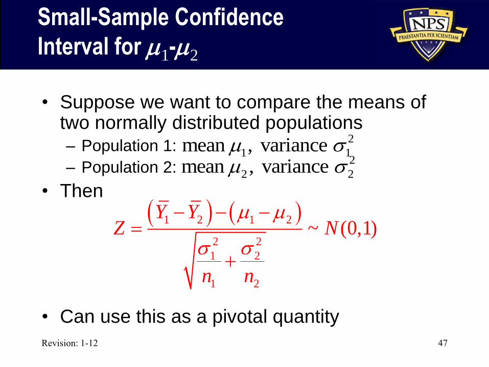
Small-Sample Confidence
Interval for m1-m2
• Suppose we want to compare the means of two normally distributed populations
– Population 1:
– Population 2:
• Then
• Can use this as a pivotal quantity
1 2 1 2
2 2
1 2
1 2
~ (0,1)Y Y
Z N
n n
m m
2
1 1mean , variance m 2
2 2mean , variance m
Revision: 1-12 48
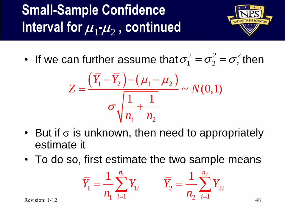
Small-Sample Confidence
Interval for m1-m2 , continued
• If we can further assume that , then
• But if is unknown, then need to appropriately estimate it
• To do so, first estimate the two sample means
1 2 1 2
1 2
~ (0,1)1 1
Y YZ N
n n
m m
2 2 2
1 2
1
1 1
11
1 n
i
i
Y Yn
2
2 2
12
1 n
i
i
Y Yn
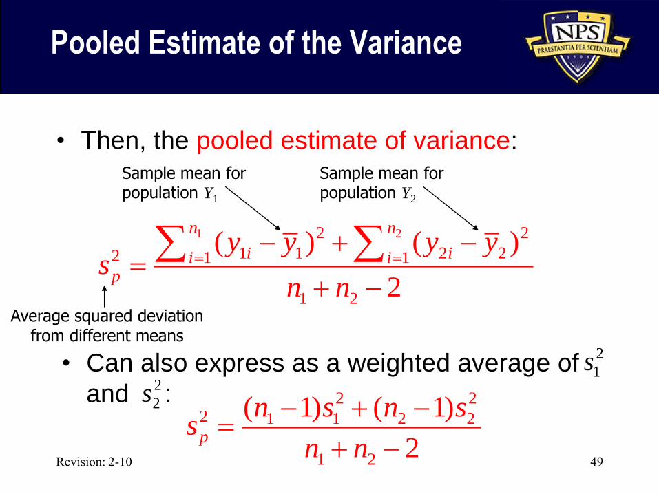
• Then, the pooled estimate of variance:
Revision: 2-10 49
1 22 2
1 1 2 22 1 1
1 2
( ) ( )
2
n n
i ii ip
y y y ys
n n
Sample mean for population Y1
Sample mean for population Y2
• Can also express as a weighted average of
and :
2
1s2
2s
Average squared deviation from different means
Pooled Estimate of the Variance
2 22 1 1 2 2
1 2
( 1) ( 1)
2p
n s n ss
n n
Revision: 1-12 50
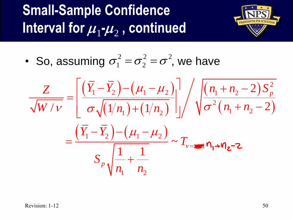
Small-Sample Confidence
Interval for m1-m2 , continued
• So, assuming , we have
2
1 2 1 2 1 2
2
1 21 2
1 2 1 2
1
1 2
2
2/ 1 1
~1 1
p
n
p
Y Y n n SZ
n nW n n
Y YT
Sn n
m m
m m
2 2 2
1 2
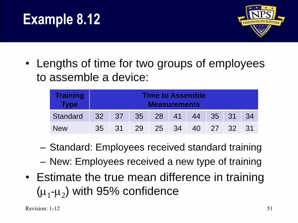
Example 8.12
• Lengths of time for two groups of employees
to assemble a device:
– Standard: Employees received standard training
– New: Employees received a new type of training
• Estimate the true mean difference in training
(m1-m2) with 95% confidence
Revision: 1-12 51
Training
Type
Time to Assemble
Measurements
Standard 32 37 35 28 41 44 35 31 34
New 35 31 29 25 34 40 27 32 31
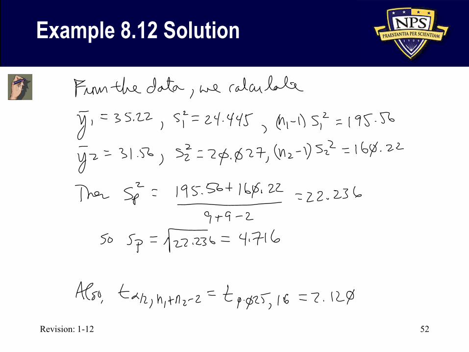
Example 8.12 Solution
Revision: 1-12 52
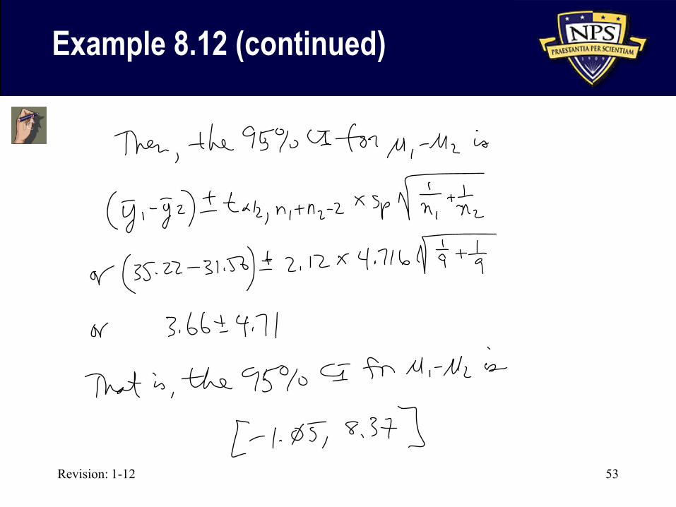
Example 8.12 (continued)
Revision: 1-12 53
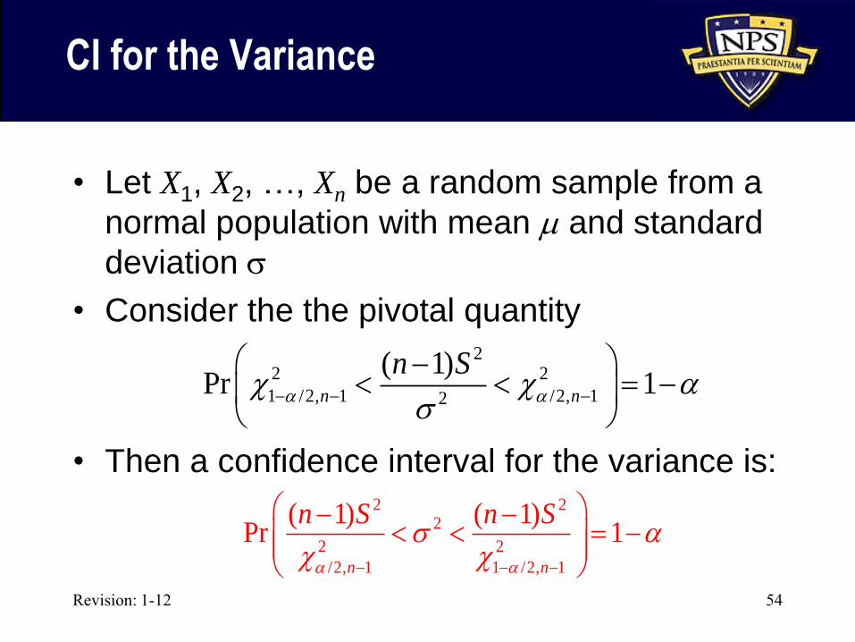
CI for the Variance
• Let X1, X2, …, Xn be a random sample from a
normal population with mean m and standard
deviation
• Consider the the pivotal quantity
• Then a confidence interval for the variance is:
Revision: 1-12 54
22 2
1 /2, 1 /2, 12
( 1)Pr 1n n
n Sa a a
2 22
2 2
/2, 1 1 /2, 1
( 1) ( 1)Pr 1
n n
n S n S
a a
a
Revision: 1-12 55
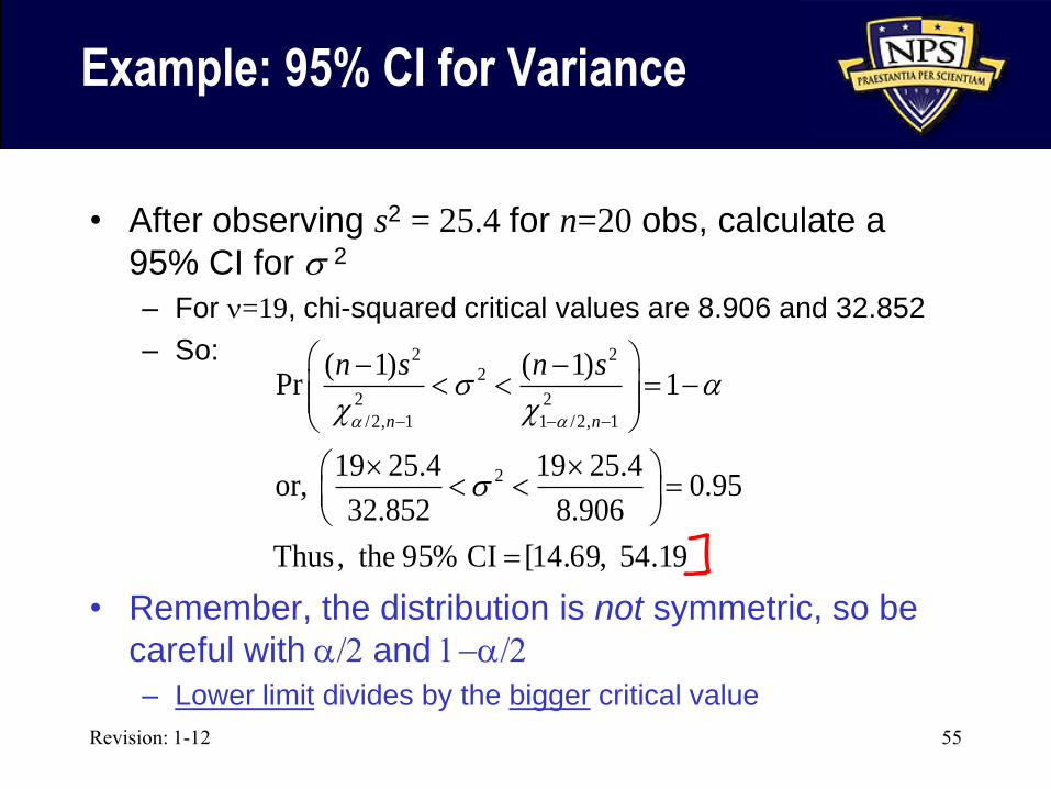
Example: 95% CI for Variance
• After observing s2 = 25.4 for n=20 obs, calculate a
95% CI for 2
– For =19, chi-squared critical values are 8.906 and 32.852
– So:
• Remember, the distribution is not symmetric, so be
careful with a and a
– Lower limit divides by the bigger critical value
2 22
2 2
/2, 1 1 /2, 1
2
( 1) ( 1)Pr 1
19 25.4 19 25.4or, 0.95
32.852 8.906
Thu s, the 95% CI [14.69, 54.19
n n
n s n s
a a
a
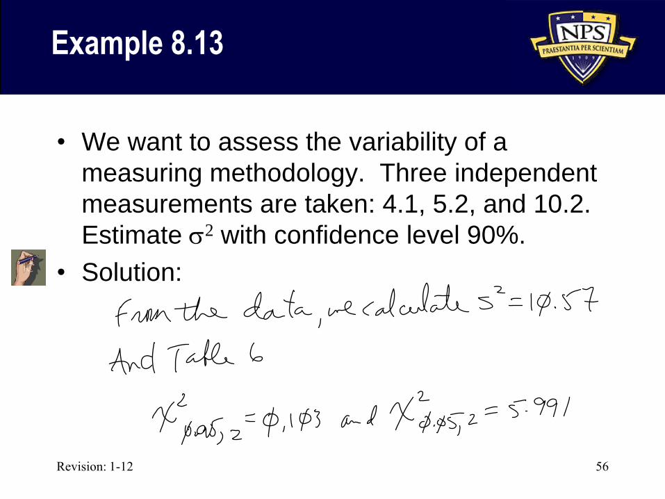
Example 8.13
• We want to assess the variability of a
measuring methodology. Three independent
measurements are taken: 4.1, 5.2, and 10.2.
Estimate 2 with confidence level 90%.
• Solution:
Revision: 1-12 56
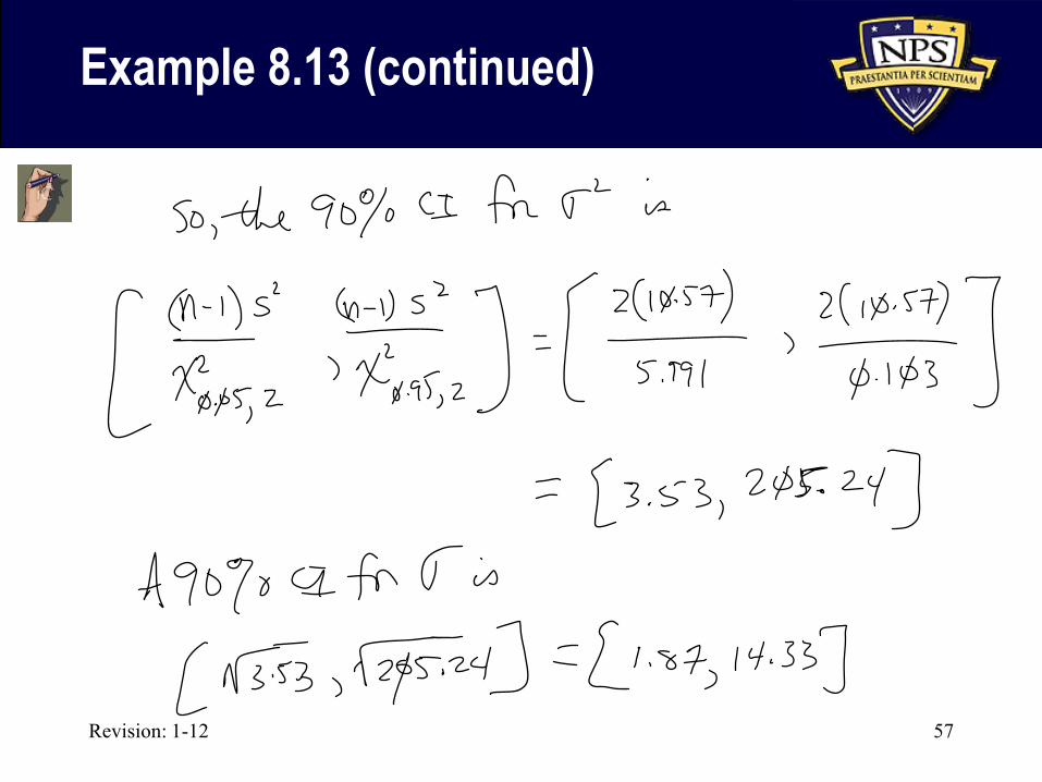
Example 8.13 (continued)
Revision: 1-12 57
Revision: 1-12 58
Why Calculate CIs for ?
• Just like with m, is a population parameter – Sometimes need to know how well it is estimated
by s
• E.g., the precision of a weapon is inversely proportional to its standard deviation – if the standard deviation is large, the weapon is not precise – Confidence intervals for provide information
about the likely range of the impact error
– Big difference between a of 3 meters and a of 300 meters with implications for both collateral damage and friendly troops
Revision: 1-12 59
Bootstrap Confidence Intervals
• Can use the bootstrap method to estimate
confidence intervals
• Basic idea:
– Use bootstrap methodology to create an empirical
sampling distribution for statistic of interest
– Then take the appropriate quantiles of the
empirical distribution for upper and lower end-
points of confidence interval
• As with point estimation, useful when it’s hard
to analytically specify sampling distribution
Revision: 1-12 60
Caution! Confidence Intervals
are Not for Prediction
• CI is an interval estimate for the population parameter
• CIs do not predict the likely range of the next observation - common pitfall!
• Interval for next observation is called a prediction interval
• Prediction interval has variability of original random variable plus the uncertainty about the population parameter
Revision: 1-12 61
• Interval estimation – i.e., confidence intervals
– Terminology
– Pivotal method for creating confidence intervals
• Types of intervals
– Large-sample confidence intervals
– One-sided vs. two-sided intervals
– Small-sample confidence intervals for the mean,
differences in two means
– Confidence interval for the variance
• Sample size calculations
What We Covered in this Module
Revision: 1-12 62
Homework
• WM&S chapter 8.5-8.9 – Required exercises: 40, 41, 42, 60, 63, 64, 71,
82, 91, 96
– Extra credit: 94
• Useful hints: Problems 8.91 and 8.96: Here’s you’re given the
raw data and must calculate the necessary
statistics first