CONFIDENCE INTERVALSpeople.stern.nyu.edu/wgreene/Statistics/ConfidenceInterval...Here are...

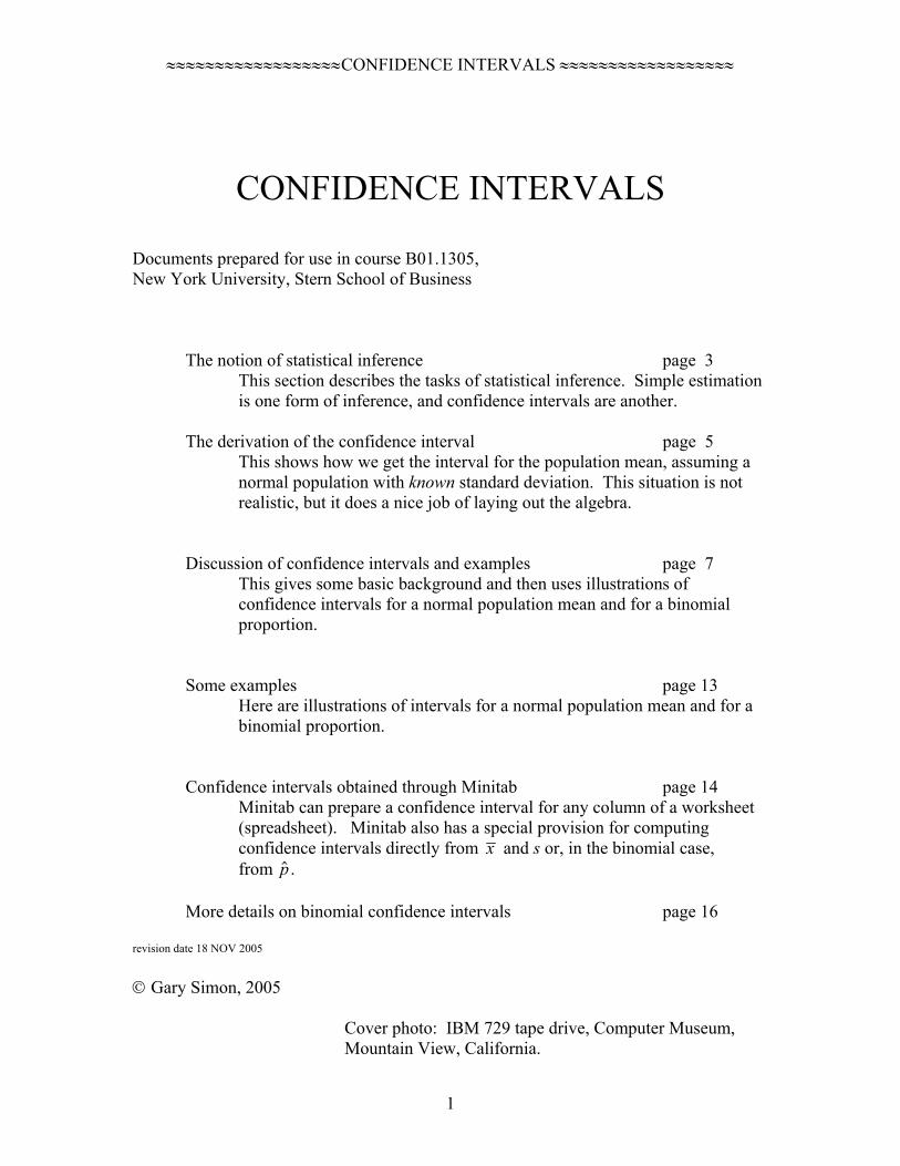
≈≈≈≈≈≈≈≈≈≈≈≈≈≈≈≈≈≈CONFIDENCE INTERVALS ≈≈≈≈≈≈≈≈≈≈≈≈≈≈≈≈≈≈

CONFIDENCE INTERVALS Documents prepared for use in course B01.1305, New York University, Stern School of Business

The notion of statistical inference page 3 This section describes the tasks of statistical inference. Simple estimation is one form of inference, and confidence intervals are another.

The derivation of the confidence interval page 5

This shows how we get the interval for the population mean, assuming a normal population with known standard deviation. This situation is not realistic, but it does a nice job of laying out the algebra.

Discussion of confidence intervals and examples page 7 This gives some basic background and then uses illustrations of confidence intervals for a normal population mean and for a binomial proportion.

Some examples page 13 Here are illustrations of intervals for a normal population mean and for a binomial proportion.

Confidence intervals obtained through Minitab page 14

Minitab can prepare a confidence interval for any column of a worksheet (spreadsheet). Minitab also has a special provision for computing confidence intervals directly from x and s or, in the binomial case, from p .

More details on binomial confidence intervals page 16

revision date 18 NOV 2005 Gary Simon, 2005

Cover photo: IBM 729 tape drive, Computer Museum, Mountain View, California.

1

≈≈≈≈≈≈≈≈≈≈≈≈≈≈≈≈≈≈CONFIDENCE INTERVALS ≈≈≈≈≈≈≈≈≈≈≈≈≈≈≈≈≈≈

2

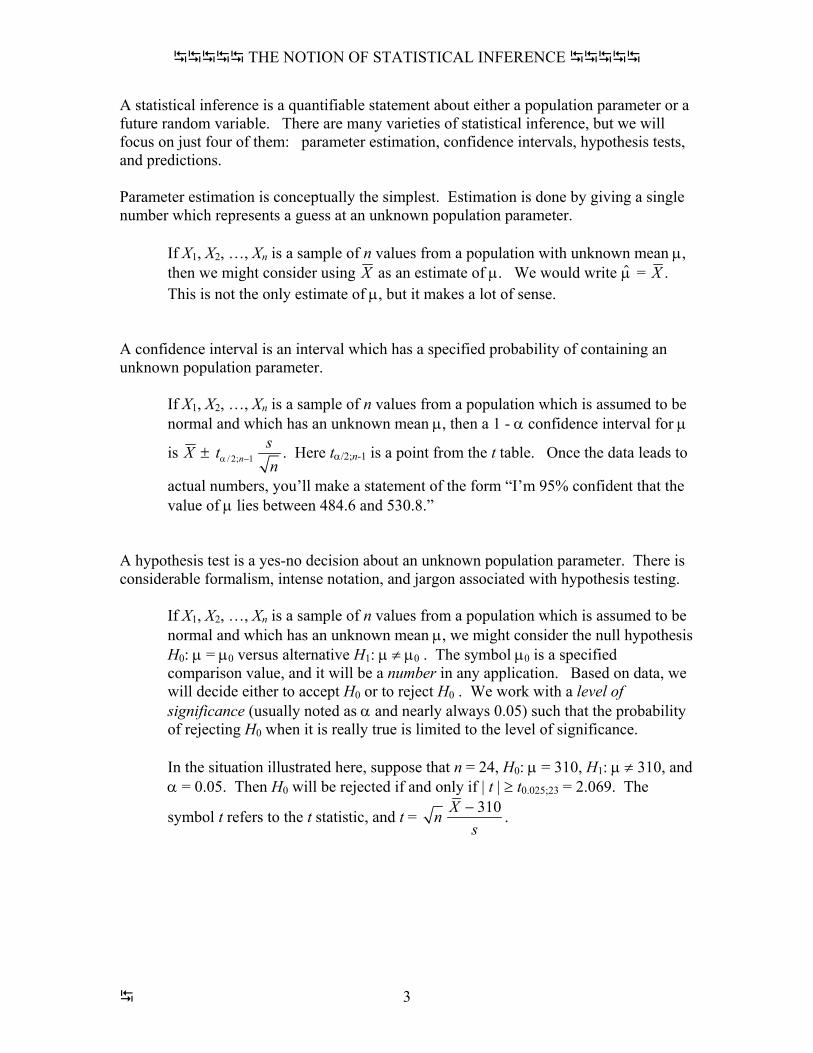
THE NOTION OF STATISTICAL INFERENCE

A statistical inference is a quantifiable statement about either a population parameter or a future random variable. There are many varieties of statistical inference, but we will focus on just four of them: parameter estimation, confidence intervals, hypothesis tests, and predictions. Parameter estimation is conceptually the simplest. Estimation is done by giving a single number which represents a guess at an unknown population parameter.

If X1, X2, …, Xn is a sample of n values from a population with unknown mean µ, then we might consider using X as an estimate of µ. We would write µ = X . This is not the only estimate of µ, but it makes a lot of sense.

A confidence interval is an interval which has a specified probability of containing an unknown population parameter.

If X1, X2, …, Xn is a sample of n values from a population which is assumed to be normal and which has an unknown mean µ, then a 1 - α confidence interval for µ

is X ± / 2; 1nsnα −t . Here tα/2;n-1 is a point from the t table. Once the data leads to

actual numbers, you’ll make a statement of the form “I’m 95% confident that the value of µ lies between 484.6 and 530.8.”

A hypothesis test is a yes-no decision about an unknown population parameter. There is considerable formalism, intense notation, and jargon associated with hypothesis testing.

If X1, X2, …, Xn is a sample of n values from a population which is assumed to be normal and which has an unknown mean µ, we might consider the null hypothesis H0: µ = µ0 versus alternative H1: µ ≠ µ0 . The symbol µ0 is a specified comparison value, and it will be a number in any application. Based on data, we will decide either to accept H0 or to reject H0 . We work with a level of significance (usually noted as α and nearly always 0.05) such that the probability of rejecting H0 when it is really true is limited to the level of significance. In the situation illustrated here, suppose that n = 24, H0: µ = 310, H1: µ ≠ 310, and α = 0.05. Then H0 will be rejected if and only if | t | ≥ t0.025;23 = 2.069. The

symbol t refers to the t statistic, and t = 310Xns− .

3

THE NOTION OF STATISTICAL INFERENCE

Predictions are guesses about values of future random variables. We can subdivide this notion into point predictions and interval predictions, but point predictions are usually obvious.

If X1, X2, …, Xn is a sample of n values from a population which is assumed to be normal and which has an unknown mean µ, we might wish to predict the next value Xn+1 . Implicit in this discussion is that we have observed X1 through Xn , but we have not yet observed Xn+1 . The point prediction is certainly X ; in fact, we would write X n+1 = X . The 1 - α prediction interval works out to be

X ± / 2; 11

nt snα − +1 .

4

THE DERIVATION OF THE CONFIDENCE INTERVAL

The normal table gives us the fact that P[ -1.96 < Z < 1.96 ] = 0.95. With a sample of n values from a population with mean µ and standard deviation σ, the

Central Limit theorem gives us the result that Z = X

n

− µσ = n X − µ

σ is approximately

normally distributed with mean 0 and with standard deviation 1.

If the population is assumed to be exactly normal to start with, then n X − µσ

is

automatically normally distributed. (This is not a use of the Central Limit theorem.) If one does not make the assumption that the population is exactly normal to start

with, then n X − µσ

is approximately normal, provided n is large enough. (This

is precisely the Central Limit theorem.) The official standard is that n should be at least 30. The result works well for n as small as 10, provided that one is not working with probabilities like 0.0062 or 0.9974 which are too close to zero or one.

Start from P[ -1.96 < Z < 1.96 ] = 0.95 and then substitute for Z the expression n X − µσ

.

This will give us

P 1.96 1.96Xn −µ − < < σ = 0.95

We can rewrite this as

P 1.96 1.96Xn nσ σ − < −µ <

= 0.95

Now subtract X from all items to get

P 1.96 1.96X Xn nσ σ − − < −µ < − +

= 0.95

Multiply by -1 (which requires reversing inequality direction) to obtain

P 1.96 1.96X Xn nσ σ + > µ > −

= 0.95

5

THE DERIVATION OF THE CONFIDENCE INTERVAL

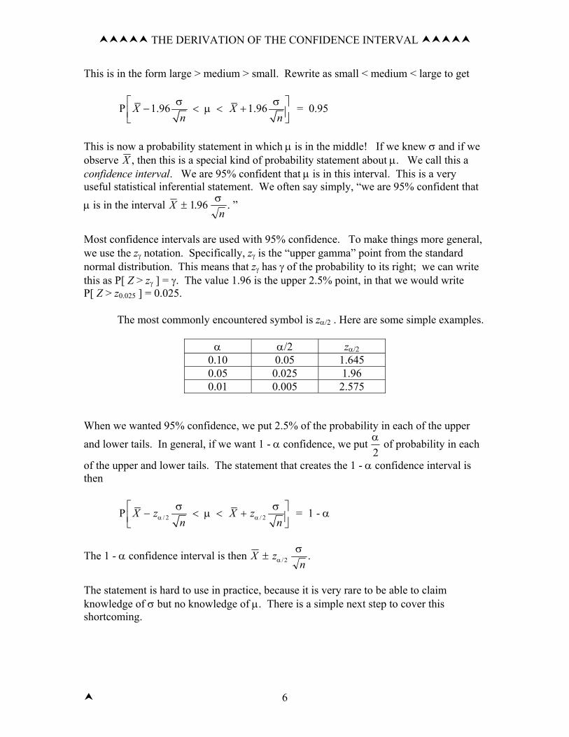
This is in the form large > medium > small. Rewrite as small < medium < large to get

P 1.96 1.96X Xn nσ σ − < µ < +

= 0.95

This is now a probability statement in which µ is in the middle! If we knew σ and if we observe X , then this is a special kind of probability statement about µ. We call this a confidence interval. We are 95% confident that µ is in this interval. This is a very useful statistical inferential statement. We often say simply, “we are 95% confident that

µ is in the interval X ± 1 9 . ” 6. σn

Most confidence intervals are used with 95% confidence. To make things more general, we use the zγ notation. Specifically, zγ is the “upper gamma” point from the standard normal distribution. This means that zγ has γ of the probability to its right; we can write this as P[ Z > zγ ] = γ. The value 1.96 is the upper 2.5% point, in that we would write P[ Z > z0.025 ] = 0.025.

The most commonly encountered symbol is zα/2 . Here are some simple examples.

α α/2 zα/2 0.10 0.05 1.645 0.05 0.025 1.96 0.01 0.005 2.575

When we wanted 95% confidence, we put 2.5% of the probability in each of the upper

and lower tails. In general, if we want 1 - α confidence, we put α2

of probability in each

of the upper and lower tails. The statement that creates the 1 - α confidence interval is then

/ 2 / 2P X z X zn nα α

σ σ − < µ < + = 1 - α

The 1 - α confidence interval is then X ± znασ

/2 .

The statement is hard to use in practice, because it is very rare to be able to claim knowledge of σ but no knowledge of µ. There is a simple next step to cover this shortcoming.

6

DISCUSSION OF CONFIDENCE INTERVALS AND EXAMPLES

A confidence interval is a statement used to trap unknown population parameters. An example....

We are 95% confident that the September mean sales per store is between 246 thousand dollars and 282 thousand dollars.

The speaker is trying to estimate µ, the true-but-unknown population mean sales per store. Presumably he or she has used a sample to make the statement. The statement is either true or false (and we don’t know which), but it would be reasonable to give 95-to-5 betting odds that the statement is true. The simplest approximate confidence interval statement is this:

We are approximately 95% confident that the unknown parameter is in the interval [estimate] ± 2 [standard error].

This is approximate for a number of reasons. First of all, we are trying to make an all-purpose statement that really might not apply perfectly to everything. Also, the “2” should really be 1.96, which has the property that P[ -1.96 ≤ Z ≤ 1.96 ] = 0.95 for a standard normal random variable Z. One can refine the statistical theory a bit, tuning up any or all of

choice for the estimate technique for obtaining the standard error

refining the multiplier “2”

Let’s give next what may be the most-commonly used confidence interval. Suppose that you have a sample X1, X2, X3, X4, …, Xn . As usual, we will use the upper case letters when we think of the Xi’s as random variables and x1, x2, x3, x4, …, xn when we think of these as observed numerical values. In practice, this distinction will be hard to enforce. The procedure which we will use depends on the assumption that the Xi values constitute a sample from a population which follows the normal distribution.

As usual, stating an assumption does not make it true. Nonetheless, it is important to state an assumption that you are going to exploit, even if you do not completely believe the assumption. It is important to invoke the conditions on which the work depends. The procedure which follows, by the way, happens to work rather well even if the sampled population does not follow the normal distribution. Moreover, when the sample size n exceeds 30, the normal distribution assumption is not critical.

Let’s use µ for the mean of the population and use σ for the standard deviation of the population. In all realistic problems, the values of µ and σ are both unknown. The statistical work will be based on the sample mean X and the sample standard deviation s.

7


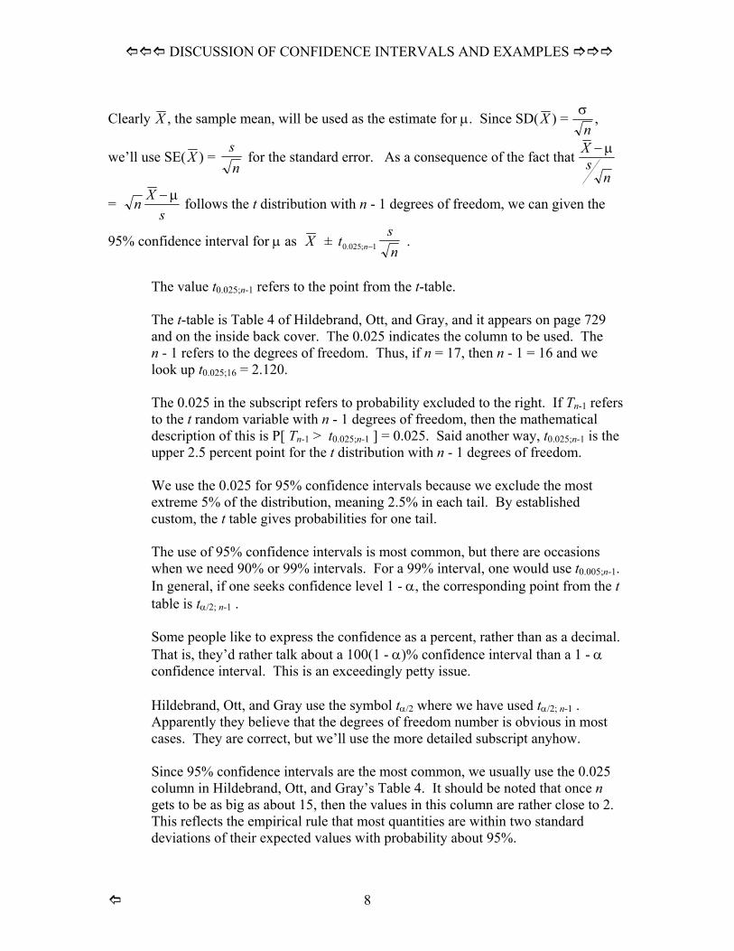
Clearly X , the sample mean, will be used as the estimate for µ. Since SD( X ) = σn

,

we’ll use SE( X ) = sn

for the standard error. As a consequence of the fact that Xs

n

− µ

= n Xs− µ follows the t distribution with n - 1 degrees of freedom, we can given the

95% confidence interval for µ as X ± tsnn0.025 1; − .

The value t0.025;n-1 refers to the point from the t-table. The t-table is Table 4 of Hildebrand, Ott, and Gray, and it appears on page 729 and on the inside back cover. The 0.025 indicates the column to be used. The n - 1 refers to the degrees of freedom. Thus, if n = 17, then n - 1 = 16 and we look up t0.025;16 = 2.120. The 0.025 in the subscript refers to probability excluded to the right. If Tn-1 refers to the t random variable with n - 1 degrees of freedom, then the mathematical description of this is P[ Tn-1 > t0.025;n-1 ] = 0.025. Said another way, t0.025;n-1 is the upper 2.5 percent point for the t distribution with n - 1 degrees of freedom. We use the 0.025 for 95% confidence intervals because we exclude the most extreme 5% of the distribution, meaning 2.5% in each tail. By established custom, the t table gives probabilities for one tail. The use of 95% confidence intervals is most common, but there are occasions when we need 90% or 99% intervals. For a 99% interval, one would use t0.005;n-1. In general, if one seeks confidence level 1 - α, the corresponding point from the t table is tα/2; n-1 . Some people like to express the confidence as a percent, rather than as a decimal. That is, they’d rather talk about a 100(1 - α)% confidence interval than a 1 - α confidence interval. This is an exceedingly petty issue. Hildebrand, Ott, and Gray use the symbol tα/2 where we have used tα/2; n-1 . Apparently they believe that the degrees of freedom number is obvious in most cases. They are correct, but we’ll use the more detailed subscript anyhow. Since 95% confidence intervals are the most common, we usually use the 0.025 column in Hildebrand, Ott, and Gray’s Table 4. It should be noted that once n gets to be as big as about 15, then the values in this column are rather close to 2. This reflects the empirical rule that most quantities are within two standard deviations of their expected values with probability about 95%.

8


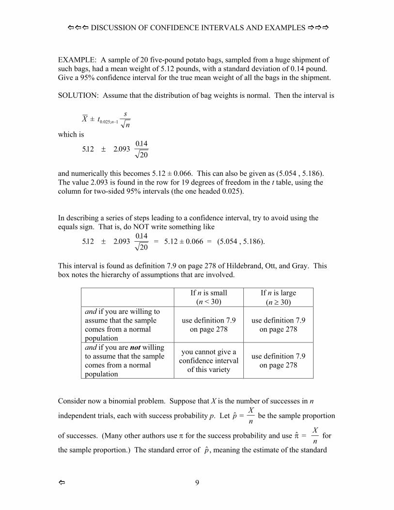
EXAMPLE: A sample of 20 five-pound potato bags, sampled from a huge shipment of such bags, had a mean weight of 5.12 pounds, with a standard deviation of 0.14 pound. Give a 95% confidence interval for the true mean weight of all the bags in the shipment. SOLUTION: Assume that the distribution of bag weights is normal. Then the interval is

X ± tsnn0.025 1; −

which is

512 2 093014

20. .

.±

and numerically this becomes 5.12 ± 0.066. This can also be given as (5.054 , 5.186). The value 2.093 is found in the row for 19 degrees of freedom in the t table, using the column for two-sided 95% intervals (the one headed 0.025). In describing a series of steps leading to a confidence interval, try to avoid using the equals sign. That is, do NOT write something like

512 2 093014

20. .

.± = 5.12 ± 0.066 = (5.054 , 5.186).

This interval is found as definition 7.9 on page 278 of Hildebrand, Ott, and Gray. This box notes the hierarchy of assumptions that are involved.

If n is small (n < 30)

If n is large (n ≥ 30)

and if you are willing to assume that the sample comes from a normal population

use definition 7.9 on page 278


and if you are not willing to assume that the sample comes from a normal population

you cannot give a confidence interval

of this variety


Consider now a binomial problem. Suppose that X is the number of successes in n

independent trials, each with success probability p. Let p = Xn

be the sample proportion

of successes. (Many other authors use π for the success probability and use π = Xn

for

the sample proportion.) The standard error of p , meaning the estimate of the standard

9


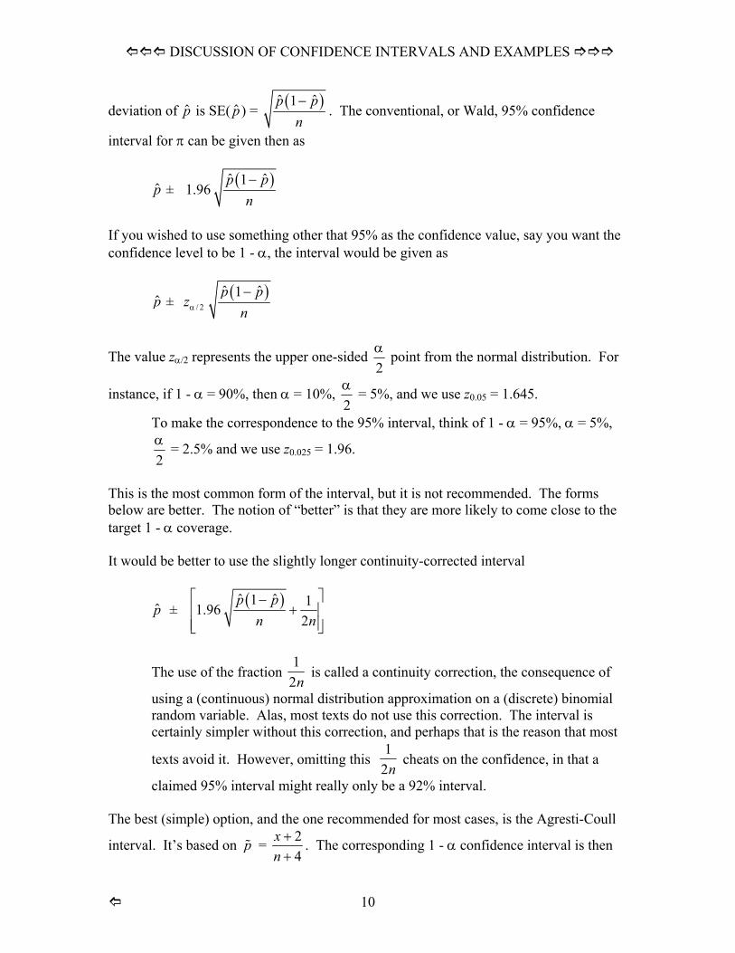
deviation of is SE( ) = p p ( )ˆ ˆ1p pn−

. The conventional, or Wald, 95% confidence

interval for π can be given then as

( )1p

1zα n

p ± ˆ ˆ

1.96p

n−

If you wished to use something other that 95% as the confidence value, say you want the confidence level to be 1 - α, the interval would be given as

p ± ( )/ 2

ˆ ˆp p−

The value zα/2 represents the upper one-sided 2α point from the normal distribution. For

instance, if 1 - α = 90%, then α = 10%, 2α = 5%, and we use z0.05 = 1.645.

To make the correspondence to the 95% interval, think of 1 - α = 95%, α = 5%,

2α = 2.5% and we use z0.025 = 1.96.

This is the most common form of the interval, but it is not recommended. The forms below are better. The notion of “better” is that they are more likely to come close to the target 1 - α coverage. It would be better to use the slightly longer continuity-corrected interval

p ± ( )ˆ ˆ1 11.962

p pn n

−+

The use of the fraction 1

2n is called a continuity correction, the consequence of

using a (continuous) normal distribution approximation on a (discrete) binomial random variable. Alas, most texts do not use this correction. The interval is certainly simpler without this correction, and perhaps that is the reason that most

texts avoid it. However, omitting this 1

2n cheats on the confidence, in that a

claimed 95% interval might really only be a 92% interval. The best (simple) option, and the one recommended for most cases, is the Agresti-Coull

interval. It’s based on p = 24

xn++

. The corresponding 1 - α confidence interval is then

10


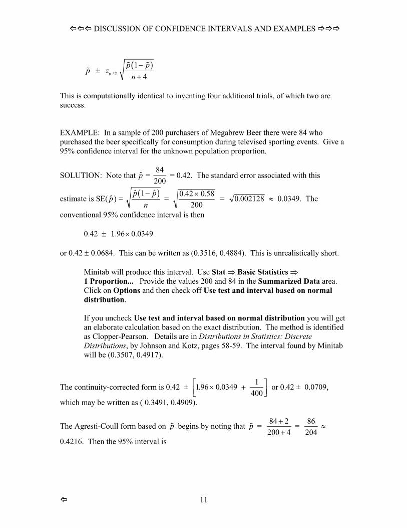
p ± ( )/ 2

14

p pz

nα

−+

This is computationally identical to inventing four additional trials, of which two are success. EXAMPLE: In a sample of 200 purchasers of Megabrew Beer there were 84 who purchased the beer specifically for consumption during televised sporting events. Give a 95% confidence interval for the unknown population proportion.

SOLUTION: Note that = p84200

= 0.42. The standard error associated with this

estimate is SE( p) = ( )ˆ 1 ˆp pn−

= 0 0 5200

.42 .× 8 = 0 002128. ≈ 0.0349. The

conventional 95% confidence interval is then

0.42 ± 1.96 0.0349× or 0.42 ± 0.0684. This can be written as (0.3516, 0.4884). This is unrealistically short.

Minitab will produce this interval. Use Stat ⇒ Basic Statistics ⇒ 1 Proportion... Provide the values 200 and 84 in the Summarized Data area. Click on Options and then check off Use test and interval based on normal distribution. If you uncheck Use test and interval based on normal distribution you will get an elaborate calculation based on the exact distribution. The method is identified as Clopper-Pearson. Details are in Distributions in Statistics: Discrete Distributions, by Johnson and Kotz, pages 58-59. The interval found by Minitab will be (0.3507, 0.4917).

The continuity-corrected form is 0.42 ± 1 96 0 0349 1400

. .× +LNM or 0.42 ± 0.0709,

which may be written as ( 0.3491, 0.4909).

OQP

The Agresti-Coull form based on p begins by noting that p = 84 2200 4

++

= 86204

≈

0.4216. Then the 95% interval is

11


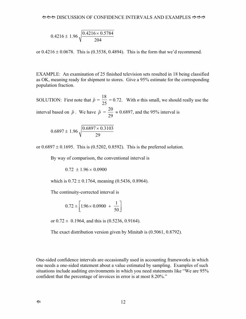
0.4216 ± 0.4216 0.5784204×1.96

or 0.4216 ± 0.0678. This is (0.3538, 0.4894). This is the form that we’d recommend. EXAMPLE: An examination of 25 finished television sets resulted in 18 being classified as OK, meaning ready for shipment to stores. Give a 95% estimate for the corresponding population fraction.

SOLUTION: First note that p = 1825

= 0.72. With n this small, we should really use the

interval based on p . We have p = 2029

≈ 0.6897, and the 95% interval is

0.6897 ± 0.6897 0.310329×1.96

or 0.6897 ± 0.1695. This is (0.5202, 0.8592). This is the preferred solution.

By way of comparison, the conventional interval is

0.72 ± 1.96 × 0.0900 which is 0.72 ± 0.1764, meaning (0.5436, 0.8964). The continuity-corrected interval is

0.72 ± 1 96 0 0900 150

. .× +L OQPNM

or 0.72 ± 0.1964, and this is (0.5236, 0.9164).

The exact distribution version given by Minitab is (0.5061, 0.8792).

One-sided confidence intervals are occasionally used in accounting frameworks in which one needs a one-sided statement about a value estimated by sampling. Examples of such situations include auditing environments in which you need statements like “We are 95% confident that the percentage of invoices in error is at most 8.20%.”

12

SOME EXAMPLES

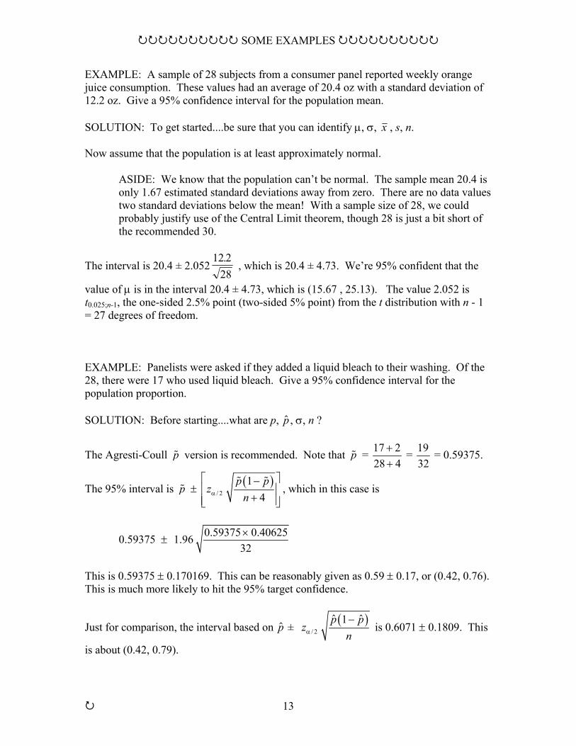
EXAMPLE: A sample of 28 subjects from a consumer panel reported weekly orange juice consumption. These values had an average of 20.4 oz with a standard deviation of 12.2 oz. Give a 95% confidence interval for the population mean. SOLUTION: To get started....be sure that you can identify µ, σ, x , s, n. Now assume that the population is at least approximately normal.

ASIDE: We know that the population can’t be normal. The sample mean 20.4 is only 1.67 estimated standard deviations away from zero. There are no data values two standard deviations below the mean! With a sample size of 28, we could probably justify use of the Central Limit theorem, though 28 is just a bit short of the recommended 30.

The interval is 20.4 ± 2.05212 2

28.

, which is 20.4 ± 4.73. We’re 95% confident that the

value of µ is in the interval 20.4 ± 4.73, which is (15.67 , 25.13). The value 2.052 is t0.025;n-1, the one-sided 2.5% point (two-sided 5% point) from the t distribution with n - 1 = 27 degrees of freedom. EXAMPLE: Panelists were asked if they added a liquid bleach to their washing. Of the 28, there were 17 who used liquid bleach. Give a 95% confidence interval for the population proportion. SOLUTION: Before starting....what are p, , σ, n ? p

The Agresti-Coull p version is recommended. Note that p = 17 228 4

++

= 1932

= 0.59375.

The 95% interval is p ± ( )/ 2

14

p pz

nα

−

+ , which in this case is

0.59375 ± 0.59375 0.4062532×1.96

This is 0.59375 ± 0.170169. This can be reasonably given as 0.59 ± 0.17, or (0.42, 0.76). This is much more likely to hit the 95% target confidence.

Just for comparison, the interval based on p ± ( )/ 2

ˆ ˆ1p pz

nα

− is 0.6071 ± 0.1809. This

is about (0.42, 0.79).

13

CONFIDENCE INTERVALS OBTAINED THROUGH MINITAB oooooooooooooooooooooooooooooooooooo

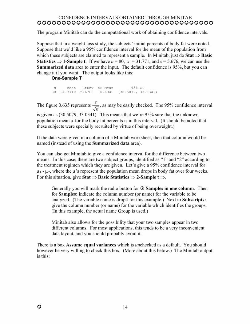
The program Minitab can do the computational work of obtaining confidence intervals. Suppose that in a weight loss study, the subjects’ initial percents of body fat were noted. Suppose that we’d like a 95% confidence interval for the mean of the population from which these subjects are claimed to represent a sample. In Minitab, just do Stat ⇒ Basic Statistics ⇒ 1-Sample t. If we have n = 80, x = 31.771, and s = 5.676, we can use the Summarized data area to enter the input. The default confidence is 95%, but you can change it if you want. The output looks like this:

One-Sample T N Mean StDev SE Mean 95% CI 80 31.7710 5.6760 0.6346 (30.5079, 33.0341)

The figure 0.635 represents sn

, as may be easily checked. The 95% confidence interval

is given as (30.5079, 33.0341). This means that we’re 95% sure that the unknown population mean µ for the body fat percents is in this interval. (It should be noted that these subjects were specially recruited by virtue of being overweight.) If the data were given in a column of a Minitab worksheet, then that column would be named (instead of using the Summarized data area). You can also get Minitab to give a confidence interval for the difference between two means. In this case, there are two subject groups, identified as “1” and “2” according to the treatment regimen which they are given. Let’s give a 95% confidence interval for µ1 - µ2, where the µ’s represent the population mean drops in body fat over four weeks. For this situation, give Stat ⇒ Basic Statistics ⇒ 2-Sample t ⇒.

Generally you will mark the radio button for Samples in one column. Then for Samples: indicate the column number (or name) for the variable to be analyzed. (The variable name is drop4 for this example.) Next to Subscripts: give the column number (or name) for the variable which identifies the groups. (In this example, the actual name Group is used.) Minitab also allows for the possibility that your two samples appear in two different columns. For most applications, this tends to be a very inconvenient data layout, and you should probably avoid it.

There is a box Assume equal variances which is unchecked as a default. You should however be very willing to check this box. (More about this below.) The Minitab output is this:

o 14

CONFIDENCE INTERVALS OBTAINED THROUGH MINITAB oooooooooooooooooooooooooooooooooooo

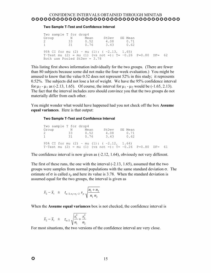
Two Sample T-Test and Confidence Interval Two sample T for drop4 Group N Mean StDev SE Mean 2 33 0.52 4.08 0.71 1 31 0.76 3.43 0.62 95% CI for mu (2) - mu (1): ( -2.13, 1.65) T-Test mu (2) = mu (1) (vs not =): T= -0.26 P=0.80 DF= 62 Both use Pooled StDev = 3.78

This listing first shows information individually for the two groups. (There are fewer than 80 subjects because some did not make the four-week evaluation.) You might be amused to know that the value 0.52 does not represent 52% in this study; it represents 0.52%. The subjects did not lose a lot of weight. We have the 95% confidence interval for µ2 - µ1 as (-2.13, 1.65). Of course, the interval for µ1 - µ2 would be (-1.65, 2.13). The fact that the interval includes zero should convince you that the two groups do not materially differ from each other. You might wonder what would have happened had you not check off the box Assume equal variances. Here is that output:

Two Sample T-Test and Confidence Interval Two sample T for drop4 Group N Mean StDev SE Mean 2 33 0.52 4.08 0.71 1 31 0.76 3.43 0.62 95% CI for mu (2) - mu (1): ( -2.12, 1.64) T-Test mu (2) = mu (1) (vs not =): T= -0.26 P=0.80 DF= 61

The confidence interval is now given as (-2.12, 1.64), obviously not very different. The first of these runs, the one with the interval (-2.13, 1.65), assumed that the two groups were samples from normal populations with the same standard deviation σ. The estimate of σ is called sp and here its value is 3.78. When the standard deviation is assumed equal for the two groups, the interval is given as

x x2 − 1 ± 1 2

1 2/ 2; 2

1 2n n p

n nt sn nα + −+

When the Assume equal variances box is not checked, the confidence interval is

x x2 − 1 ± z sn

snα /2

12

1

22

2

+

For most situations, the two versions of the confidence interval are very close.

o 15

MORE DETAILS ON BINOMIAL CONFIDENCE INTERVALS T T T T T T T T T T T T T T T T T T T T T T T T T T T T T

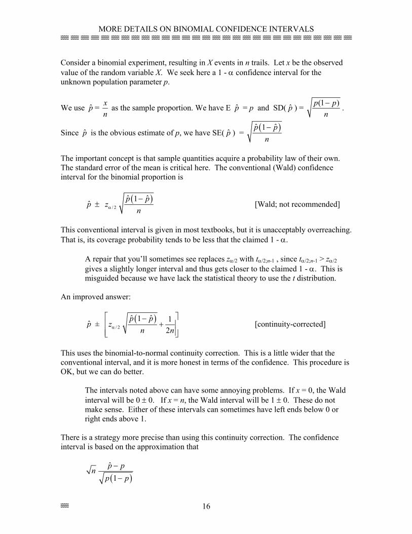
Consider a binomial experiment, resulting in X events in n trails. Let x be the observed value of the random variable X. We seek here a 1 - α confidence interval for the unknown population parameter p.

We use p̂ = xn

as the sample proportion. We have E p̂ = p and SD( p̂ ) = (1 )p pn− .

Since p̂ is the obvious estimate of p, we have SE( p̂ ) = ( )ˆ ˆ1p pn−

The important concept is that sample quantities acquire a probability law of their own. The standard error of the mean is critical here. The conventional (Wald) confidence interval for the binomial proportion is

p̂ ± ( )/ 2

ˆ ˆ1p pz

nα

− [Wald; not recommended]

This conventional interval is given in most textbooks, but it is unacceptably overreaching. That is, its coverage probability tends to be less that the claimed 1 - α.

A repair that you’ll sometimes see replaces zα/2 with tα/2;n-1 , since tα/2;n-1 > zα/2 gives a slightly longer interval and thus gets closer to the claimed 1 - α. This is misguided because we have lack the statistical theory to use the t distribution.

An improved answer:

p̂ ± ( )/ 2

ˆ ˆ1 12

p pz

n nα

−+

[continuity-corrected]

This uses the binomial-to-normal continuity correction. This is a little wider that the conventional interval, and it is more honest in terms of the confidence. This procedure is OK, but we can do better.

The intervals noted above can have some annoying problems. If x = 0, the Wald interval will be 0 ± 0. If x = n, the Wald interval will be 1 ± 0. These do not make sense. Either of these intervals can sometimes have left ends below 0 or right ends above 1.

There is a strategy more precise than using this continuity correction. The confidence interval is based on the approximation that

( )ˆ

1p pn

p p−

−

T 16


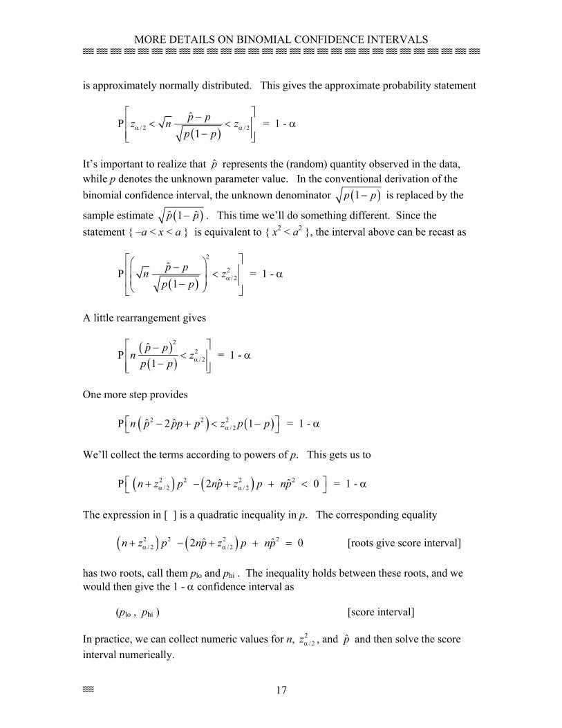
is approximately normally distributed. This gives the approximate probability statement

( )/ 2 / 2ˆ

P1

p pz n zp pα α

− < <

− = 1 - α

It’s important to realize that p̂ represents the (random) quantity observed in the data, while p denotes the unknown parameter value. In the conventional derivation of the binomial confidence interval, the unknown denominator ( )1p p− is replaced by the

sample estimate ( )ˆ 1 ˆp p− . This time we’ll do something different. Since the statement { –a < x < a } is equivalent to { x2 < a2 }, the interval above can be recast as

( )

2

2/ 2

ˆP

1p pn z

p p α

− < −

= 1 - α

A little rearrangement gives

( )( )

22

/ 2

ˆP

1p p

np p α

−<

− z

)

0

= 1 - α

One more step provides

( ) (2 2 2/ 2ˆ ˆP 2 1n p pp p z p pα

− + < − = 1 - α

We’ll collect the terms according to powers of p. This gets us to

( ) ( )2 2 2 2/ 2 / 2ˆ ˆP 2n z p np z p npα α

+ − + + < = 1 - α

The expression in [ ] is a quadratic inequality in p. The corresponding equality

( ) ( )2 2 2 2/ 2 / 2ˆ ˆ2n z p np z p npα α+ − + + 0= [roots give score interval]

has two roots, call them plo and phi . The inequality holds between these roots, and we would then give the 1 - α confidence interval as

(plo , phi ) [score interval] In practice, we can collect numeric values for n, 2

/ 2zα , and p̂ and then solve the score interval numerically.

T 17


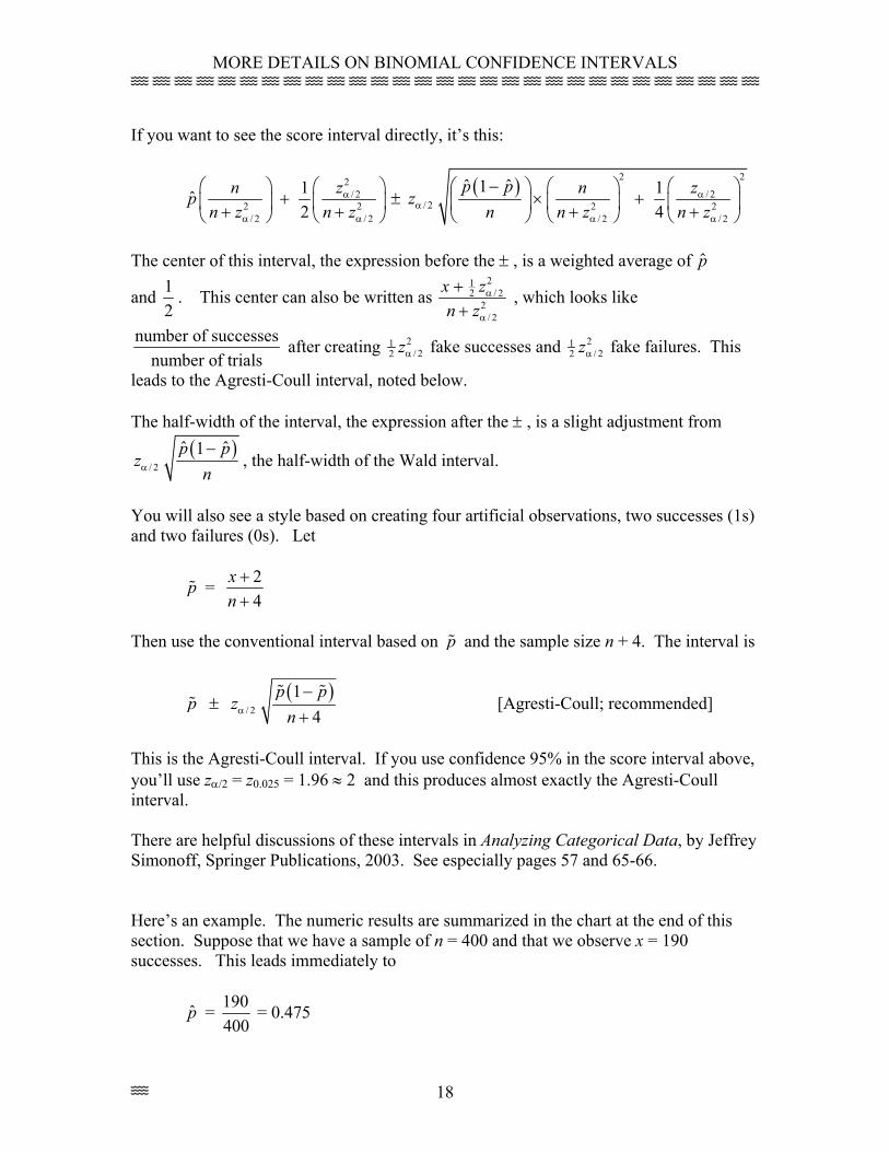
If you want to see the score interval directly, it’s this:

2/ 2

2 2/ 2 / 2

1ˆ2

n zpn z n z

α

α α

+ + +

± ( ) 2 2

/ 2/ 2 2 2

/ 2 / 2

ˆ ˆ1 14

p p n zzn n z n z

αα

α α

− × + + +

The center of this interval, the expression before the ± , is a weighted average of p

and 12

. This center can also be written as 21

2 / 22

/ 2

x zn z

α

α

++

, which looks like

number of successesnumber of trials

after creating 21/ 22 zα fake successes and 21

/ 22 zα fake failures. This

leads to the Agresti-Coull interval, noted below. The half-width of the interval, the expression after the ± , is a slight adjustment from

( )/ 2

ˆ ˆ1p pz

nα

−, the half-width of the Wald interval.

You will also see a style based on creating four artificial observations, two successes (1s) and two failures (0s). Let

p = 24

xn++

Then use the conventional interval based on p and the sample size n + 4. The interval is

p ± ( )/ 2

14

p pz

nα

−+

[Agresti-Coull; recommended]

This is the Agresti-Coull interval. If you use confidence 95% in the score interval above, you’ll use zα/2 = z0.025 = 1.96 ≈ 2 and this produces almost exactly the Agresti-Coull interval. There are helpful discussions of these intervals in Analyzing Categorical Data, by Jeffrey Simonoff, Springer Publications, 2003. See especially pages 57 and 65-66. Here’s an example. The numeric results are summarized in the chart at the end of this section. Suppose that we have a sample of n = 400 and that we observe x = 190 successes. This leads immediately to

p̂ = 190400

= 0.475

T 18


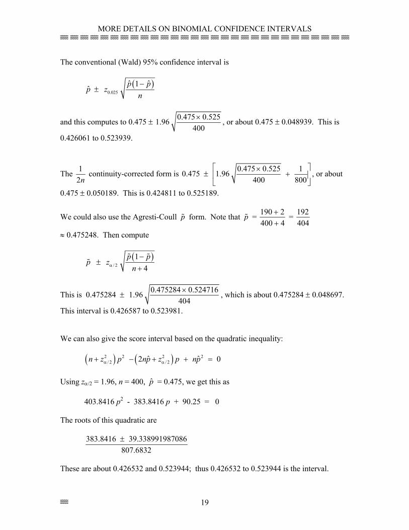
The conventional (Wald) 95% confidence interval is

p̂ ± ( )0.025

ˆ ˆ1p pz

n−

and this computes to 0.475 ± 0.475 0.525400×1.96 , or about 0.475 ± 0.048939. This is

0.426061 to 0.523939.

The 12n

continuity-corrected form is 0.475 0.525 11.96400 800

0.475 ×

± +

, or about

0.475 ± 0.050189. This is 0.424811 to 0.525189.

We could also use the Agresti-Coull p form. Note that p = 190 2400 4

++

= 192404

≈ 0.475248. Then compute

p ± ( )/ 2

14

p pz

nα

−+

This is 0.475284 ± 0.475284 0.524716404×1.96 , which is about 0.475284 ± 0.048697.

This interval is 0.426587 to 0.523981. We can also give the score interval based on the quadratic inequality:

( ) ( )2 2 2 2/ 2 / 2ˆ ˆ2 0n z p np z p npα α+ − + + =

Using zα/2 = 1.96, n = 400, p̂ = 0.475, we get this as

403.8416 p2 - 383.8416 p + 90.25 = 0 The roots of this quadratic are

383.8416 39.338991987086807.6832±

These are about 0.426532 and 0.523944; thus 0.426532 to 0.523944 is the interval.

T 19


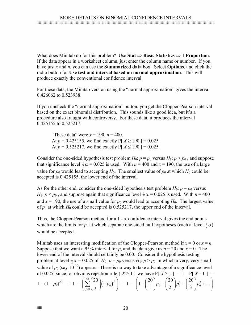
What does Minitab do for this problem? Use Stat ⇒ Basic Statistics ⇒ 1 Proportion. If the data appear in a worksheet column, just enter the column name or number. If you have just x and n, you can use the Summarized data box. Select Options, and click the radio button for Use test and interval based on normal approximation. This will produce exactly the conventional confidence interval. For these data, the Minitab version using the “normal approximation” gives the interval 0.426062 to 0.523938. If you uncheck the “normal approximation” button, you get the Clopper-Pearson interval based on the exact binomial distribution. This sounds like a good idea, but it’s a procedure also fraught with controversy. For these data, it produces the interval 0.425155 to 0.525217.

“These data” were x = 190, n = 400. At p = 0.425155, we find exactly P[ X ≥ 190 ] = 0.025. At p = 0.525217, we find exactly P[ X ≤ 190 ] = 0.025.

Consider the one-sided hypothesis test problem H0: p = p0 versus H1: p > p0 , and suppose that significance level 1

2 α = 0.025 is used. With n = 400 and x = 190, the use of a large value for p0 would lead to accepting H0. The smallest value of p0 at which H0 could be accepted is 0.425155, the lower end of the interval. As for the other end, consider the one-sided hypothesis test problem H0: p = p0 versus H1: p < p0 , and suppose again that significance level 1

2 α = 0.025 is used. With n = 400 and x = 190, the use of a small value for p0 would lead to accepting H0. The largest value of p0 at which H0 could be accepted is 0.525217, the upper end of the interval. Thus, the Clopper-Pearson method for a 1 - α confidence interval gives the end points which are the limits for p0 at which separate one-sided null hypotheses (each at level 1

2 α) would be accepted. Minitab uses an interesting modification of the Clopper-Pearson method if x = 0 or x = n. Suppose that we want a 95% interval for p, and the data give us n = 20 and x = 0. The lower end of the interval should certainly be 0.00. Consider the hypothesis testing problem at level 1

2 α = 0.025 of H0: p = p0 versus H1: p > p0 in which a very, very small value of p0 (say 10-10) appears. There is no way to take advantage of a significance level of 0.025, since for obvious rejection rule { X ≥ 1 } we have P[ X ≥ 1 ] = 1 – P[ X = 0 ] =

1 – (1 – p0)20 = 1 = 1 ( )

20

00

20 j

j

pj=

− −

∑ 2 3

0 0 0

20 20 201 ...

1 2 3p p p

− − + − +

T 20


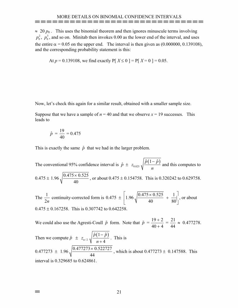
≈ 20 p0 . This uses the binomial theorem and then ignores minuscule terms involving 20p , 3

0p , and so on. Minitab then invokes 0.00 as the lower end of the interval, and uses the entire α = 0.05 on the upper end. The interval is then given as (0.000000, 0.139108), and the corresponding probability statement is this:

12n

At p = 0.139108, we find exactly P[ X ≤ 0 ] = P[ X = 0 ] = 0.05.

Now, let’s check this again for a similar result, obtained with a smaller sample size. Suppose that we have a sample of n = 40 and that we observe x = 19 successes. This leads to

p̂ = 1940

= 0.475

This is exactly the same p̂ that we had in the larger problem.

The conventional 95% confidence interval is p̂ ± ( )0.025

ˆ ˆ1p pz

n−

and this computes to

0.475 ± 0.475 0.52540×1.96 , or about 0.475 ± 0.154758. This is 0.320242 to 0.629758.

The continuity-corrected form is 0.475 0.525 11.9640 80

0.475 ×

± +

, or about

0.475 ± 0.167258. This is 0.307742 to 0.642258.

We could also use the Agresti-Coull p form. Note that p = 19 240 4

++

= 2144

≈ 0.477278.

Then we compute p ± ( )/ 2

14

p pz

nα

−+

. This is

0.477273 ± 0.477273 0.52272744×1.96 , which is about 0.477273 ± 0.147588. This

interval is 0.329685 to 0.624861.

T 21


T 22

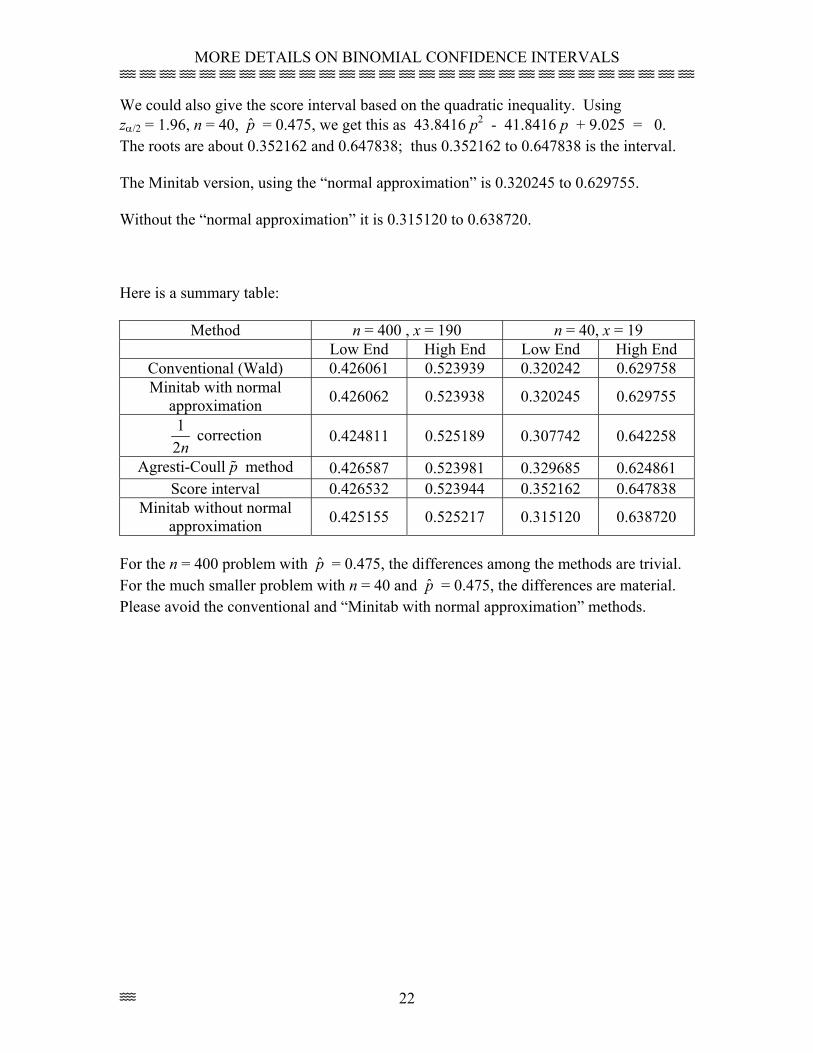
We could also give the score interval based on the quadratic inequality. Using zα/2 = 1.96, n = 40, p̂ = 0.475, we get this as 43.8416 p2 - 41.8416 p + 9.025 = 0. The roots are about 0.352162 and 0.647838; thus 0.352162 to 0.647838 is the interval. The Minitab version, using the “normal approximation” is 0.320245 to 0.629755. Without the “normal approximation” it is 0.315120 to 0.638720. Here is a summary table:

Method n = 400 , x = 190 n = 40, x = 19 Low End High End Low End High End

Conventional (Wald) 0.426061 0.523939 0.320242 0.629758 Minitab with normal

approximation 0.426062 0.523938 0.320245 0.629755

12n

correction 0.424811 0.525189 0.307742 0.642258

Agresti-Coull p method 0.426587 0.523981 0.329685 0.624861 Score interval 0.426532 0.523944 0.352162 0.647838

Minitab without normal approximation 0.425155 0.525217 0.315120 0.638720

For the n = 400 problem with p̂ = 0.475, the differences among the methods are trivial. For the much smaller problem with n = 40 and p̂ = 0.475, the differences are material. Please avoid the conventional and “Minitab with normal approximation” methods.

CONFIDENCE INTERVALSpeople.stern.nyu.edu/wgreene/Statistics/ConfidenceInterval...Here are...

Documents

Transcript of CONFIDENCE INTERVALSpeople.stern.nyu.edu/wgreene/Statistics/ConfidenceInterval...Here are...