Conducting studies of the microbiota - UAB

Conducting studies of the microbiota

Matthew Stoll MD,PhD,MSCS

MIC741

January 22, 2016

Outline

• Where and how to sample

• Sequencing

• Data analysis

Multiple habitats

Harris, Jrnl Obesity 2012;2012:879151

Bacteria composition differs by site

HMP Consortium, Nature 2012;486:207

Heterogeneity within habitats

• Gut

• Skin

• Mouth

Fecal vs mucosal microbiota

Mucosal Fecal

Rangel, Aliment Pharmacol Ther 2015;42:1211

Unprepped sigmoid biopsies

Affect of washout

Jalanka, Gut 2015;64:1562

Spatial heterogeneity in intestines

Mao, Scientific Reports 2015;5:16116

Cecu

m

Co

lon

R

ectu

m

Fecal microbiota

• Patient prepares own sample

– Usually at home

• Shipment

$25 payment $50 payment

Received / Promised 27 / 62 (44%) 128 / 178 (72%)

Money helps

Sample preparation

• Can get small amounts with used toilet

paper

• I prefer to use a stool collection device

(“hat”), subject transfers to collection vial

• Carey-Blair media (permits growth of live

bacteria), if functional studies are planned

• Send overnight via commercial carrier

Skin has topographically distinct

microbiota

Findley, Nature 2013;498:367

Heel

Elbow

Back

Skin collection

• Consistency with respect to personal

hygeine measures (bathing, lotions,

perfumes, topical antibiotics, etc.)

• Two methods

– Cotton swab x 15 seconds (easier)

– Skin scrapings using sterile blade (higher

yield)

Mouth also has topographically

distinct microbiota

Buccal mucosa

Keratinized gingiva

Hard palate

Throat

Tonsils

Tongue Dorsum

Saliva

Supragingival plaque

Subgingival plaque

Segata, Genome Biol 2012;13:R42

Oral cavity collection

• Saliva

• Cotton swab

• Gingival plaque

Genitourinary

• Sample collection swab

– HMP: Collected by study team

– Alternative: self-collection

Useful information to collect

• Diet (fecal microbiota)

• Antibiotics

• Skin and oral hygeine products

• Menstrual cycle and contraceptive use

(reproductive tract microbiota)

DNA preparation

• Various kits used for DNA purification

– MoBio tubes preferred by HMP

– We used Zymo for fecal collection

• Key is that you need conditions harsh

enough to lyse the microbes

Outline


• Sequencing

• Data analysis

Type of sequencing

More information Less cost

Whole genome sequencing

Species of strain information

Functional potential

16S sequencing

Genus information

No direct functional potential

• Amplification of 16S ribosomal DNA

• Whole genome sequencing

Cost comparison of 16S and WGS

• An Illumina flow cell costs about $1000

• Can handle 100 16S samples

– Avg cost of $10; ~ $15 including PCR

– Currently subsidized by UAB

• The same flow cell runs only 3 WGS samples

– Creating the library and additional expenses bring it close to $900 / sample

• Higher informatics costs

Sequencing prep in one slide

16S (Peter Eipers PhD)

• PCR of 16S region

• Special primers

– Barcode at one end

– Adaptor at other

WGS (Mike Crowley PhD)

• Shear DNA

• Ligate adaptors to each end

– Includes barcodes

• Short PCR

• Optional size selection

Starting with purified DNA

Cyclic reversible termination

Incorporate all four nucleotides, each with different dye

Metzker, Nature Rev Genet 2010;11:31


Wash out unused nucleotides; image



Cleave dye and terminating groups



Back to step one


Barcodes to sort out samples

Sample 1: AGGTTCCA

Sample 2: GGCAATTT

Sample 3: TTGGAAAC

Trends in sequencing cost

Snyder, Genes & Dev.

2010;42:423

Outline


• Sequencing

• Data analysis

Output: fastq files

Header: @M02079:147:000000000-AK0J5:1:1101:15736:1676 1:N:0:49

Sequence: TACAGAGGTCTCAAGCGTTGTTCGGAATCACTGGGCGTAA

Additional line: +

Quality: >//>>EEGGFFE/////<//>-<0>DBF1<F<1.<<-<GD

Header: @M02079:147:000000000-AK0J5:1:1101:15989:1722 1:N:0:49

Sequence: TACGGAGGATGCGAGCGTTATCCGGATTTATTGGGTTTAAAG

Additional line: +

Quality: B3EHFGGHF3FB43/E?EFGGFFGH3/B4?//B/FG?122FB

Sample Fastq output (two DNA strands)

Assess quality of reads

Position in read (BP)

Qu

ality

sco

re

0

10

20

30

40

Managing paired reads

16S sequencing

• PCR output is 250 – 300 bp in length

• Illumina MiSeq produces 250 bp paired-end reads

5’ 3’

5’ 3’

F R

F and R reads should be identical in

area of overlap

Paired reads do not always

overlap

WGS sequencing

Fragments may be 400 – 500 bp

Sequence output may be shorter,

and may not overlap

Quality control and merger of

paired end reads

• If there is substantial overlap, the

merging itself is a QC step

• If the reads disagree on a base call, the

program accepts the base with a higher

associated quality score

• User can input minimal amount of

overlap, number of permissible errors

Quality control and merger of

paired end reads

• If there is NOT substantial overlap, the

paired reads cannot be merged

• Need to use programs that apply the

QC steps to both the forward and

reverse reads

– If one is removed, its mate must also be

removed

Quality filtering options

• Trim the low-quality tails

– Option: remove sequence if more than a set percentage of bases are trimmed

• Remove sequences with a certain number of ambiguous bases

• Remove sequences which have quality scores below a threshold

– Can permit a set percentage (e.g. remove if 5% have q-scores < 30).

Convert to fasta

• Fasta files do not have quality information

• Are used for most analyses

Fasta sequences

Header: >M02079:147:000000000-AK0J5:1:1101:15736:1676 1:N:0:49

Sequence: TACAGAGGTCTCAAGCGTTGTTCGGAATCACTGGGCGTAA

Header: >M02079:147:000000000-AK0J5:1:1101:15989:1722 1:N:0:49

Sequence: TACGGAGGATGCGAGCGTTATCCGGATTTATTGGGTTTAAAG

16S data analysis

• Different programs exist for 16S analysis

– Mothur

– Quantitative Insight into Microbial Ecology

(QIIME)

QIIME • Open-source bioinformatics pipeline

• Designed for 16S sequence analysis

• Every step from fastq processing through data analysis

• Coming soon: QIIME 2 – GUI

– Better support for whole genome sequencing

www.QIIME.org

The OTU table

• Analyses are performed on the

“operational taxonomic unit (OTU)” table,

not the fasta sequence file

• OTUs are groups of similar sequences

– User can set the similarity; 97% is standard

• Matter of efficiency (may have 2 million

sequences, just 3000 OTUs)

• Clearly, OTU picking is essential step

Biom format of OTU table

• Information contained in OTU table

– List of sample IDs (subj 1, subj 2, etc)

– List of OTU IDs

– Frequency of each OTU in each sample

– Optional: taxonomy

• Earlier versions of QIIME had OTU tables in .txt format

• Biom format has same information, but can store more data

• Not particularly intuitive to look at

Closed vs open reference OTU

picking strategies

OTU picking

strategy

Compare

with existing

database

Speed Inclusion of

new taxa

CLOSED

REFERENCE

YES Faster No

OPEN

REFERENCE

NO Slower Yes

QIIME offers a hybrid approach

• Script: pick_open_reference_otus.py

• User inputs database; default option is the

latest greengenes release

– Curation of all the 16S reference sequences

– Has associated taxonomy file

Greengenes fasta and taxa files

>1111881

GCTGGCGGCGTGCCTAACACATGTAAGTCGAACGGGAC

TGGGGGCAACTCCAGTTCAGTGGCAGACGGGTGCGT

>1111882

AGAGTTTGATCATGGCTCAGGATGAACGCTAGCGGCAG

GCCTAACACATGCAAGTCGAGGGGTAGAGGCTTTCG

1111882 k__Bacteria; p__Bacteroidetes; c__Flavobacteriia;

o__Flavobacteriales; f__Flavobacteriaceae; g__Flavobacterium; s__

Greengenes fasta

Greengenes taxonomy 1111881 k__Bacteria; p__Proteobacteria; c__Epsilonproteobacteria;

o__Campylobacterales; f__Helicobacteraceae; g__; s__

pick_open_reference_otus.py

Closed ref OTU picking against greengenes

Input fasta file

Greengenes

OTU 1

OTU 2

Closed ref failures


Open ref OTU picking with the failures

Closed ref failures

OTU 3

Open ref failure

Sequence is discarded


Make OTU table and pick reference set

OTU clustering

Reference set of

fasta sequences

Biom table


• Add taxonomy information to biom table

– Again using greengenes by default

• Take representative fasta set

– Align against greengenes files

– Generate phylogenetic tree

Final steps

What do you do with the biom

table?

Not much, if you don’t have a metadata file

Contents of metadata file

• Subject IDs

– Whatever is printed on tube with DNA

– This will be name of output fastq file

– Be sure to follow HIPAA

• Important metadata

– Disease status

– Treatment

– Sex

– etc.

Metadata file

#SampleID Disease Sex Antibiotics

Subj1 Arthritis Male No

Subj2 Arthritis Male No

Subj3 Arthritis Female Yes

Subj4 Control Female No

Subj5 Control Female No

Subj6 Control Male No

#SampleID should be header of the first column

What do you do with the biom

table?

• Show taxonomy

• Alpha diversity (within group)

• Beta diversity (between group)

• Comparisons

First, get summary information

• biom summarize-table -i otu_table.biom

-o summary.txt

• Creates a .txt file which includes:

– Sample IDs included in file

– Sequencing depth of each ID

– Number of samples

– Number of OTUs

Assigning taxonomy

• assign.taxonomy.py -i rep_set.fasta -t greengenes_97_otus.txt -r greengenes_97_otus.fasta -m uclust – Generates a .txt file with two columns: OTU

and taxonomy

– One row for each OTU

– Info can be incorporated into OTU table

• summarize_taxa.py -i otu_table.biom -o taxa/ – Creates a set of .biom and .txt files for each

taxonomy level (by default, L2 - L6)

Displaying taxonomy

Alpha diversity

• Richness: number of different species

present in a sample

• Evenness: how evenly dispersed these

species are

Alpha diversity

Rich and even Rich, not even Not rich or even

Phylogenetic alpha diversity

• Takes into account the phylogenetic

tree and similarity between species

• A mixture of bacteria from different

phyla is seen as more diverse than, say,

20 different species of staphylococcus

Cautionary note about

measuring alpha diversity

• Must take into account sequencing depth

• Typically, at UAB, depth is 50K – 150K

sequences per sample for 16S

• To a point, diversity increases with higher

depth, as you pick up more rare species

• Rarefaction curves often are shown

Illustration of rarefaction curves

Measuring alpha diversity in QIIME

• Step 1. Perform rarefactions, selecting which sequencing depth or depths will be evaluated

• Generally the highest should be lower than the lowest sequencing depth of your samples

• multiple_rarefactions.py -m 10000 -x 70000 -s 10000 -n 10 -i otu_table.biom -o rarefactions/


• Step 2. Run alpha diversity at each

rarefaction

• alpha_diversity.py -i rarefactions/ -o

alpha/ -t rep_set.tre -m

shannon,simpson,PD_whole_tree,chao1


• Step 3. Collate into individual files for

each metric

• collate_alpha.py -i alpha/ -o

alpha_collated/

• Output is multiple text files (one for each

metric) consisting of tables listing the

alpha diversity measurements for each

subject at each rarefaction

Sample alpha diversity output

Sequence Iteration Subj1 Subj2 Subj3

10000 1 6.9 4.2 6.8

10000 2 7.1 3.8 8.0

10000 3 7.05 3.9 8.1

20000 1 8.4 6.1 8.5

20000 2 8.2 6.2 8.2

20000 3 8.1 6.0 8.0

30000 1 8.3 6.1 8.4

30000 2 8.4 6.3 8.2

30000 3 8.4 5.9 8.3

Beta diversity

• This speaks to the diversity between

two different groups

• To analyze this, the metadata file is

essential

• QIIME can present beta diversity in the

form of a PCOA plot

• Again, consider rarefactions /

sequencing depth

Beta diversity script

• beta_diversity_through_plots.py -i

otu_table.biom -e 70000 -o beta/ -t rep_set.tre

-m map.txt

• Note that the metrics were not specified here

• For QIIME workflow scripts (which do

multiple steps at once), some options are

specified by a separate parameter file (-p

QIIME_parameters.txt)

Sample distance matrix

C1 C2 C3 C4 T1 T2 T3

C1 0 0.35 0.31 0.39 0.88 0.79 0.91

C2 0.35 0 0.42 0.22 0.92 0.90 0.74

C3 0.31 0.42 0 0.35 0.74 0.79 0.91

C4 0.39 0.22 0.35 0 0.82 0.84 0.92

T1 0.88 0.92 0.74 0.82 0 0.29 0.21

T2 0.79 0.90 0.79 0.84 0.29 0 0.32

T3 0.91 0.74 0.91 0.92 0.21 0.32 0

Sample distance matrix

C1 C2 C3 C4 T1 T2 T3

C1 0 0.35 0.31 0.39 0.88 0.79 0.91

C2 0 0.42 0.22 0.92 0.90 0.74

C3 0 0.35 0.74 0.79 0.91

C4 0 0.82 0.84 0.92

T1 0 0.29 0.21

T2 0 0.32

T3 0

Comparisons

• QIIME can perform statistical comparisons

• Input files

– Metadata file

– Distance matrix or OTU table

• Two basic flavors

– Global

– Pairwise for each OTU

• Both have multiple options for statistical tests

– Parametric or non-parametric

– Dichotomous or continuous

Comparisons

• Global compare_categories.py -i

weighted_unifrac_dm.txt -m map.txt -c Disease -o

Results/ --method permanova

– Provides a single p-value as to whether overall, the distance

matrix shows differences based upon the selected metadata

category

• Pairwise group_significance.py -i otu_table.biom -

m map.txt -c Disease -s kruskal_wallis -o

kruskal_wallis_output.txt

– Performs pairwise testing of each OTU present in the biom

table, using the selected metadata category

– Outputs p-values, plus corrected (FDR and Bonferroni)

LEfSe: widely used tool for

pairwise comparisons

• Can be performed on output at OTU or

taxonomy level

• Uses Linear Discriminant Analysis to

calculate effect size (LEfSe)

• Available on Curtis Huttenhower’s galaxy

page – https://huttenhower.sph.harvard.edu/galaxy/root

• Outputs data in tabular and graphical form

https://huttenhower.sph.harvard.edu/galaxy/root


Whole genome sequencing

• Shotgun sequencing of all the DNA

present in a sample

• May not include viral particles

• Will include human contaminant DNA

Removal of host DNA sequences

• Not required with 16S analysis

– Host DNA should not be amplified

• Contamination can occur with WGS

– Variable with fecal microbes

– High likelihood with other habitats

Assembly

• Most packages not designed for microbiota

– Thousands of species

• Unclear if needed with large reads

• Generally de novo

• Consider metAmos

– Assembles with multiple packages

– Determines optimal parameters for each

Options for host DNA removal

• Reference database of microbial

organisms

– Include sequences that align with dominant

bacteria

– Output will be limited to these bacteria

• Reference database of host DNA

– Filter out alignments

– BLAST or Bowtie2 / BWA

Assigning taxonomy

• Comparison-based

–Compare to database of sequences

• Composition-based

– Internal structure

Comparison based

• Align each sequence with reference gene

or protein databases

• Gold standard is BLAST

• Derivative programs (BLAT, mega-BLAST

and RAPSearch) increase efficiency, with

acceptable loss of accuracy

• At UAB, we use RAPSearch, then MEGAN

to assign taxonomy to the alignment files

Metaphlan for taxonomy

assignment

• Assigns taxonomy based upon marker

genes (in essence, polymorphisms)

• Metaphlan 2 includes 17000 reference

genomes with 1 million marker genes

• Includes bacterial, viral, and fungal

genomes

• Fast!

• Outputs .biom tables or .txt files

Composition based taxonomy

• Bacteria have unique sequence features

– GC content

– Nucleotide repeats

– Codon usage

Functional annotation

• Alignment with BLAST

• Annotation with KEGG or other

databases that link proteins to

metabolic functions and pathways

• HUMAnN is a popular program that can

tabulate the BLAST results

Functional annotation with 16S data

• 16S data provides taxonomic information

• Can infer function through taxonomy

• Phylogenetic Investigation of

Communities by Reconstruction of

Unobserved States (PICRUSt)

• This and other programs are available at

Curtis Huttenhower’s Harvard Galaxy site





Microbiota data

• Studied pediatric subjects with a form

of juvenile idiopathic arthritis (JIA)

• This form, called spondyloarthritis, has

clinical and genetic overlap with

inflammatory bowel disease

• Comparator group are healthy children

Taxonomy

Fra

cti

on

of

tota

l b

acte

ria

Juvenile SpA Controls

Stoll, Arth Res Ther 2014;16:486

PCoA identified a small cluster

Blue: patients

Red: controls


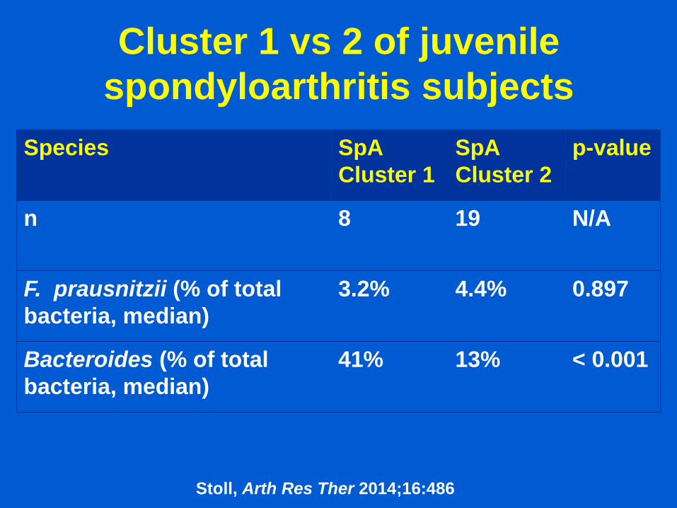
Cluster 1 vs 2 of juvenile

spondyloarthritis subjects

Species SpA

Cluster 1

SpA

Cluster 2

p-value

n 8 19 N/A

F. prausnitzii (% of total

bacteria, median)

3.2% 4.4% 0.897

Bacteroides (% of total

bacteria, median)

41% 13% < 0.001


Altered F. prausnitzii is largely

limited to SpA subtype

Stoll, Clin Immunol 2015;159:134

Fra

cti

on

of

tota

l b

acte

ria

Juvenile SpA JIA; not SpA Controls

16S sequencing in SpA: summary

• Differences at taxonomic level identified

• 16S sequencing does not provide

functional information

– Educated guesses are possible: F. prausnitzii

is a major butyrate producer

• We proceeded to assess enteric bacteria

at the functional level

– Whole genome sequencing

– Fecal water metabolomics

Lower alpha diversity in patients

Controls SpA

Taxonomic differences Higher in controls Higher in SpA

HUMAnN output: iPath2.0 Red: Higher in controls

Blue: higher in SpA

Differentially present ions

Higher in Controls

Higher in spondyloarthritis

Retention time

Mas

s :

ch

arg

e

Pathways represented in controls

Pathway Overlap p

Butanoate metabolism 2 0.05127

Tryptophan metabolism 2 0.0982

Aspartate and asparagine

metabolism 2 0.00587

Bile acid biosynthesis 2 0.01256

Xenobiotics metabolism 2 0.01668

Tyrosine metabolism 2 0.03864

Differentially present ions

Higher in Controls

Higher in spondyloarthritis

Retention time

Mas

s :

ch

arg

e

Pathways represented in controls

Pathway Overlap p

Biopterin metabolism 2 0.00042

Tryptophan metabolism 3 0.00198

Glycerophospholipid metabolism 2 0.00206

Urea cycle 2 0.00405

Tyrosine metabolism 3 0.01106

Drug metabolism - cytochrome P450 6 0.00171

N-Glycan biosynthesis 2 0.00313

Ubiquinone Biosynthesis 2 0.00507

Hexose phosphorylation 2 0.00777

Linoleate metabolism 2 0.00777

Histidine metabolism 2 0.01597

Drug metabolism - other enzymes 2 0.01867

Galactose metabolism 2 0.02839

Squalene and cholesterol biosynthesis 2 0.02839

Glycerophospholipid metabolism 2 0.04056

Tryptophan metabolism

Anti-inflammatory

Anti-inflammatory

Metabolomics and

metagenomics of SpA: summary

• Patients had lower diversity at the taxonomic, genetic, and metabolic level

• Patients had decreased metabolites from the Tryptophan metabolism pathway

• Patients had increased genes coding for tryptophanase, which results in production of indole

– Alterations in Trytophan metabolism may be associated with disease

Questions?

Conducting studies of the microbiota - UAB

Documents

Transcript of Conducting studies of the microbiota - UAB