Conducting Human-Subject Experiments with...

Conducting Human-Subject Experiments with Virtual and Augmented Reality

J. Edward Swan II, Naval Research Laboratory (organizer)

Joseph L. Gabbard, Virginia Tech

Deborah Hix, Virginia Tech

Steve Ellis, NASA Ames

Bernard D. Adelstein, NASA Ames

VR 2004 Tutorial

2

Schedule

SteveHuman Performance Studies in Virtual Environments1.0 hours200 PM

EdFinal Questions and Discussion0.5 hours430 PM

DovPsychophysics: Classical Methods1.0 hours330 PM

Coffee Break0.5 hours300 PM

EdExperimental Design and Analysis0.5 hours130 PM

Lunch Break1.5 hours1200 PM

EdExperimental Design and Analysis 1.5 hours1030 AM

Coffee Break0.5 hours1000 AM

Joe, DebbyUsability Engineering1.6 hours830 AM

EdIntroduction and Overview0.4 hours800 AM

3

Outline• Empiricism• Experimental Validity• Usability Engineering• Experimental Design• Gathering Data• Describing Data

– Graphing Data– Descriptive Statistics

• Inferential Statistics– Hypothesis Testing– Hypothesis Testing Means– Power– Analysis of Variance and Factorial Experiments

4

Why Human Subject (HS) Experiments?• VR and AR hardware/software more mature• Focus of field:

– Implementing technology → using technology• Increasingly running HS experiments:

– How do humans perceive, manipulate, cognate with VR, AR-mediated information?

– Measure utility of AR / VR for applications

• HS experiments at VR 2003:– 10/29 papers (35%)– 5/14 posters (36%)

5

Logical Deduction vs. Empiricism• Logical Deduction

– Analytic solutions in closed form– Amenable to proof techniques– Much of computer science fits here– Examples:

• Computability (what can be calculated?)• Complexity theory (how efficient is this algorithm?)

• Empirical Inquiry– Answers questions that cannot be proved

analytically– Much of science falls into this area– Antithetical to mathematics, computer science

6

What is Empiricism?• The Empirical Technique

– Develop a hypothesis, perhaps based on a theory– Make the hypothesis testable– Develop an empirical experiment– Collect and analyze data– Accept or refute the hypothesis– Relate the results back to the theory– If worthy, communicate the results to your community

• Statistics: – Foundation for empirical work; necessary but not

sufficient– Often not useful for managing problems of gathering,

interpreting, and communicating empirical information.

7

Where is Empiricism Used?• Humans are very non-analytic• Fields that study humans:

– Psychology / social sciences– Industrial engineering– Ergonomics– Business / management– Medicine

• Fields that don’t study humans:– Agriculture, natural sciences, etc.

• Computer Science:– HCI– Software engineering

8

Experimental Validity• Empiricism• Experimental Validity• Usability Engineering• Experimental Design• Gathering Data• Describing Data



9

Designing Valid Empirical Experiments• Experimental Validity

– Does experiment really measure what we want it to measure?

– Do our results really mean what we think (and hope) they mean?

– Are our results reliable?• If we run the experiment again, will we get the same

results? • Will others get the same results?

• Validity is a large topic in empirical inquiry– Usability Engineering can greatly enhance

validity of VR / AR experiments

10

Experimental Variables• Independent Variables

– What the experiment is studying– Occur at different levels

• Example: stereopsis, at the levels of stereo, mono– Systematically varied by experiment

• Dependent Variables– What the experiment measures– Assume dependent variables will be effected by

independent variables– Must be measurable quantities

• Time, task completion counts, error counts, survey answers, scores, etc.

• Example: VR navigation performance, in total time

11

Experimental Variables • Independent variables can vary in two ways

– Between-subjects: each subject sees a different level of the variable• Example: ½ of subjects see stereo, ½ see mono

– Within-subjects: each subject sees all levels of the variable• Example: each subject sees both stereo and mono

• Confounding factors (or confounding variables)– Factors that are not being studied, but will still affect

experiment• Example: stereo condition less bright than mono condition

– Important to predict and control confounding factors, or experimental validity will suffer

12

Usability Engineering• Empiricism• Experimental Validity• Usability Engineering• Experimental Design• Gathering Data• Describing Data



13

Experimental Design• Empiricism• Experimental Validity• Usability Engineering• Experimental Design• Gathering Data• Describing Data



14

Experimental Designs

• Important confounding factors for within subject variables:– Learning effects– Fatigue effects

• Control these by counterbalancing the design– Ensure no systematic variation between levels and the order

they are presented to subjects

• 2 x 1 is simplest possible design, with one independent variable at two levels:

level 2

level 1

Variable

mono

stereo

Stereopsis

mono

stereo

1st condition

2, 4, 6, 8

1, 3, 5, 7

Subjects

stereo

mono

2nd condition

15

Factorial Designs• n x 1 designs generalize the number of levels:

• Factorial designs generalize number of independent variables and the number of levels of each variable

• Examples: n x m design, n x m x p design, etc. • Must watch for factorial explosion of design size!

mountainoushillyflat

VE terrain type

Stereopsis3 x 2 design:monostereo


VE terrain type

16

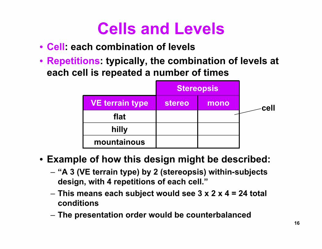
Cells and Levels• Cell: each combination of levels• Repetitions: typically, the combination of levels at

each cell is repeated a number of times

• Example of how this design might be described:– “A 3 (VE terrain type) by 2 (stereopsis) within-subjects

design, with 4 repetitions of each cell.”– This means each subject would see 3 x 2 x 4 = 24 total

conditions– The presentation order would be counterbalanced

Stereopsis

monostereo


VE terrain type cell

17

Counterbalancing• Addresses time-based confounding factors:

– Within-subjects variables: control learning and fatigue effects– Between-subjects variables: control calibration drift, weather,

other factors that vary with time

• There are two counterbalancing methods:– Random permutations– Systematic variation

• Latin squares are a very useful and popular technique

• Latin square properties:– Every level appears in

every position the same number of times

– Every level is followed by every other level

– Every level is preceded by every other level

⎥⎦

⎤⎢⎣

⎡1221

⎥⎥⎥⎥⎥⎥⎥⎥

⎦

⎤

⎢⎢⎢⎢⎢⎢⎢⎢

⎣

⎡

123213132312231321

⎥⎥⎥⎥

⎦

⎤

⎢⎢⎢⎢

⎣

⎡

1234241331424321

2 x 2

6 x 3 (there is no 3 x 3)

4 x 4

18

Counterbalancing Example• “A 3 (VE terrain type) by 2 (stereopsis) within-

subjects design, with 4 repetitions of each cell.”• Form Cartesian product of Latin squares

{6 x 3} (VE Terrain Type) ⊗ {2 x 2} (Stereopsis)• Perfectly counterbalances groups of 12 subjects

3B, 3A, 2B, 1A, 1B, 1A123A, 3B, 2A, 2B, 1A, 1B113B, 3A, 1B, 1A, 2B, 2A103A, 3B, 1A, 1B, 2A, 2B92B, 2A, 3B, 3A, 1B, 1A82A, 2B, 3A, 3B, 1A, 1B72B, 2A, 1B, 1A, 3B, 3A62A, 2B, 1A, 1B, 3A, 3B51B, 1A, 3B, 3A, 2B, 2A41A, 1B, 3A, 3B, 2A, 2B1B, 1A, 2B, 2A, 3B, 3A1A, 1B, 2A, 2B, 3A, 3B

Presentation Order

321

Subject

⎥⎥⎥⎥⎥⎥⎥⎥

⎦

⎤

⎢⎢⎢⎢⎢⎢⎢⎢

⎣

⎡

123213132312231321

⎥⎦

⎤⎢⎣

⎡ABBA

19

Experimental Design Example #1

• All variables within-subjectFrom [Living et al. 03]

20

Experimental Design Example #2

• Mixed design: some variables between-subject, others within-subject.

Com

puter Platform

offonStereo Viewing

Betw

een Subject

positionratepositionrateControl Movement

Within Subject

subjects 17 –20

ego

subjects 21 –24

exo

subjects 13 –16

exo

subjects 25 –28

ego

desktop

workbench

wall

subjects 29 –32

subjects 9 –12

subjects 5 –8

subjects 1 –4

cave

exoegoexoegoFrame of Reference

From [Swan et al. 03]

21

Gathering Data• Empiricism• Experimental Validity• Usability Engineering• Experimental Design• Gathering Data• Describing Data



22

Gathering Data• Some unique aspects of VR and AR

– Can capture, log, and analyze head trajectory– If we log head / hand trajectory so we can play it back,

must have way of logging critical incidents– VR / AR equipment more fragile than other UI setups

– In a CAVE:• Observing a subject can break their presence / immersion• Determining button presses when experimenter cannot see

wand

– In AR, very difficult to know what user is seeing• Can mount separate display near user or on their back • Could mount lightweight camera on user’s head

23

Graphing Data• Empiricism• Experimental Validity• Usability Engineering• Experimental Design• Gathering Data• Describing Data



24

Types of Statistics• Descriptive Statistics

– Describe and explore data– Summary statistics:

many numbers → few numbers– All types of graphs and visual representations– Data analysis begins with descriptive stats

• Understand data distribution• Test assumptions of significance tests

• Inferential Statistics– Detect relationships in data– Significance tests– Infer population characteristics from sample

characteristics

25

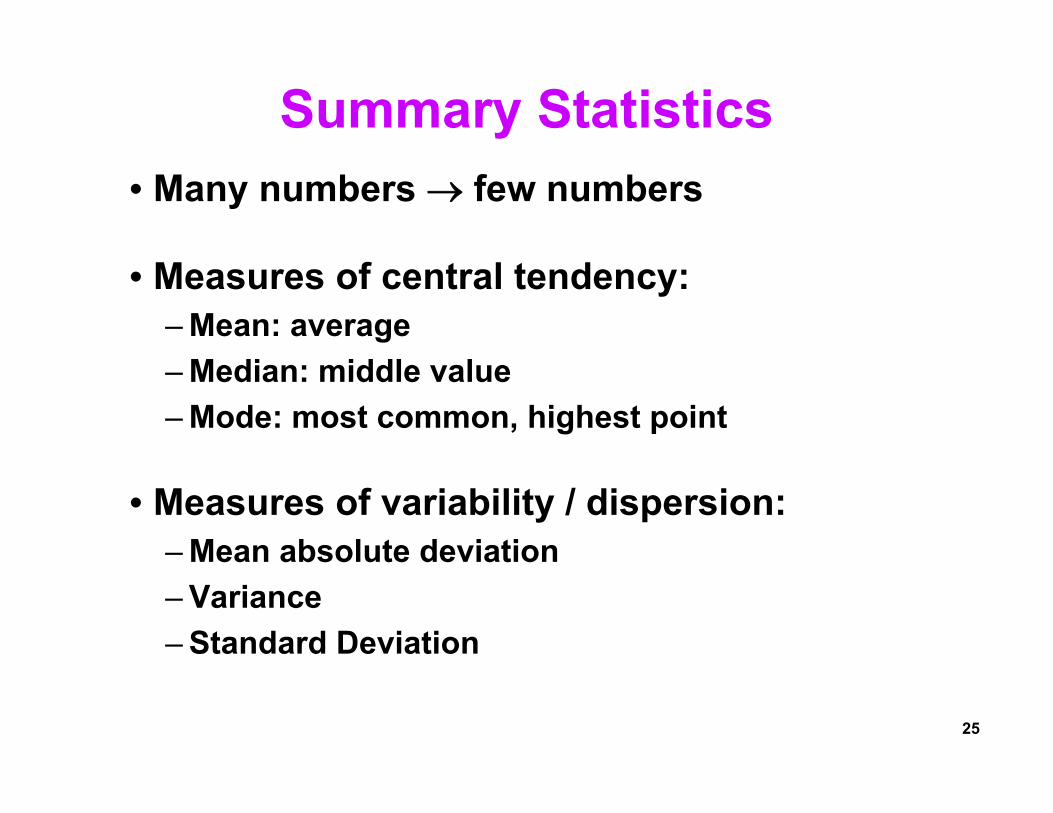
Summary Statistics• Many numbers → few numbers

• Measures of central tendency:– Mean: average– Median: middle value– Mode: most common, highest point

• Measures of variability / dispersion:– Mean absolute deviation– Variance– Standard Deviation

26

Exploring Data with Graphs• Histogram common data overview method

From

[How

ell 0

2] p

21

mode = 62median = 59.5 mean = 60.26

27

Classifying Data with Histograms

From [Howell 02] p 28

28

Stem-and-Leaf: Histogram From Actual Data

From

[How

ell 0

2] p

21,

23

29

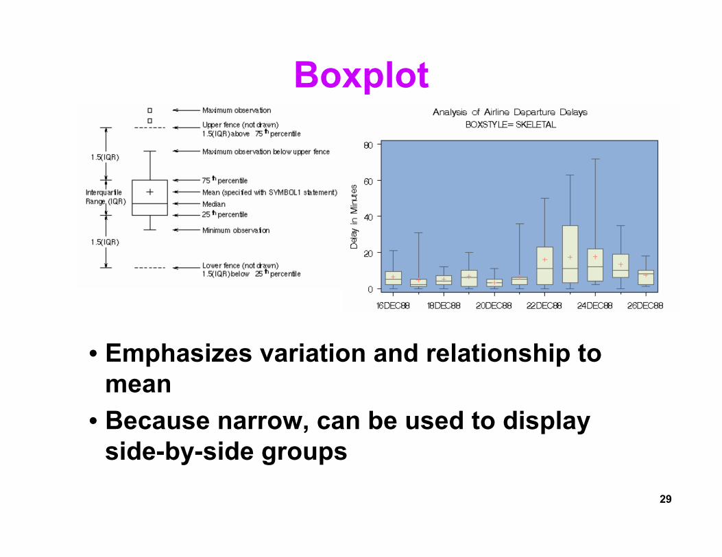
Boxplot

• Emphasizes variation and relationship to mean

• Because narrow, can be used to display side-by-side groups

30

Example Histogram and Boxplot from Real Data

mean = 2355

min value

median = 1453

25th 75th upper fence max values (outliers)

Data from [Living et al. 03]

31

We Have Only Scratched the Surface…• There are a vary large number of graphing techniques• Tufte’s [83, 90] works are classic, and stat books show many

more examples (e.g. Howell [03]).

From [Tufte 83], p 134, 62Lots of good examples…And plenty of bad examples!

32

Descriptive Statistics• Empiricism• Experimental Validity• Usability Engineering• Experimental Design• Gathering Data• Describing Data



33

• Population: – Set containing every possible element that we

want to measure– Usually a Platonic, theoretical construct– Mean: μ Variance: σ2 Standard deviation: σ

• Sample:– Set containing the elements we actually

measure (our subjects)– Subset of related population– Mean: Variance: s2 Standard deviation: s

Number of samples: N

Populations and Samples

X

34

Measuring Variability / Dispersion

• Standard deviation uses same units as samples and mean.

• Calculation of population variance σ2 is theoretical, because μ almost never known and the population size N would be very large (perhaps infinity).

N

XX∑ −=m.a.d.

Mean absolute deviation:

( )1

2

2

−−

= ∑N

XXs

Variance:

( )1

2

−−

= ∑N

XXs

Standard deviation:

Mean:

NX

X ∑=

( )N

X∑ −=

22 μ

σ

35

Sums of Squares, Degrees of Freedom,Mean Squares

• Very common terms and concepts

• Sums of squares: – Summed squared deviations from mean

• Degrees of freedom: – Given a set of N observations used in a calculation, how

many numbers in the set may vary– Equal to N minus number of means calculated

• Mean squares:– Sums of squares divided by degrees of freedom– Another term for variance, used in ANOVA

( )squares)(mean MS

freedom of degreessquares of sumsSS

1

2

2 ===−−

= ∑dfN

XXs

36

Hypothesis Testing• Empiricism• Experimental Validity• Usability Engineering• Experimental Design• Gathering Data• Describing Data



37

Hypothesis Testing• Goal is to infer population characteristics

from sample characteristics

From [Howell 02], p 78

population

samples

38

Testable Hypothesis• General hypothesis: The research question

that motivates the experiment.

• Testable hypothesis: The research question expressed in a way that can be measured and studied.

• Generating a good testable hypothesis is a real skill of experimental design.– By good, we mean contributes to experimental

validity.– Skill best learned by studying and critiquing

previous experiments.

39

Testable Hypothesis Example• General hypothesis: Stereo will make people more effective

when navigating through a virtual environment (VE).

• Testable hypothesis: We measure time it takes for subjects to navigate through a particular VE, under conditions of stereo and mono viewing. We hypothesis subjects will be faster under stereo viewing.

• Testable hypothesis requires a measurable quantity:– Time, task completion counts, error counts, etc.

• Some factors effecting experimental validity:– Is VE representative of something interesting

(e.g., a real-world situation)?– Is navigation task representative of something interesting?– Is there an underlying theory of human performance that can

help predict the results? Could our results contribute to this theory?

40

What Are the Possible Alternatives? • Let time to navigate be μs: stereo time; μm: mono time

– Perhaps there are two populations: μs – μm = d

– Perhaps there is one population: μs – μm = 0

μs μm μs μm(they could be close together)

(they could be far apart)

μs,μm

41

Hypothesis Testing Procedure1. Develop testable hypothesis H1: μs – μm = d

– (E.g., subjects faster under stereo viewing)

2. Develop null hypothesis H0: μs – μm = 0– Logical opposite of testable hypothesis

3. Construct sampling distribution assuming H0 is true.

4. Run an experiment and collect samples; yielding sampling statistic X.– (E.g., measure subjects under stereo and mono conditions)

5. Referring to sampling distribution, calculate conditional probability of seeing X given H0: p( X | H0 ).– If probability is low (p ≤ 0.05, p ≤ 0.01), we are unlikely to see X

when H0 is true. We reject H0, and embrace H1.– If probability is not low (p > 0.05), we are likely to see X when

H0 is true. We do not reject H0.

42

Example 1: VE Navigation with Stereo Viewing1. Hypothesis H1: μs – μm = d

– Subjects faster under stereo viewing.

2. Null hypothesis H0: μs – μm = 0– Subjects same speed whether stereo or mono viewing.

3. Constructed sampling distribution assuming H0 is true.

4. Ran an experiment and collected samples:– 32 subjects, collected 128 samples– Xs = 36.431 sec; Xm = 34.449 sec; Xs – Xm = 1.983 sec

5. Calculated conditional probability of seeing 1.983 sec given H0: p( 1.983 sec | H0 ) = 0.445.– p = 0.445 not low, we are likely to see 1.983 sec when H0 is

true. We do not reject H0. – This experiment did not tell us that subjects were faster under

stereo viewing.

Dat

a fr

om [S

wan

et a

l. 03

]

43

Example 2: Effect of Intensity on AR Occluded Layer Perception

1. Hypothesis H1: μc – μd = d– Tested constant and decreasing intensity. Subjects faster

under decreasing intensity.

2. Null hypothesis H0: μc – μd = 0– Subjects same speed whether constant or decreasing intensity.

3. Constructed sampling distribution assuming H0 is true.

4. Ran an experiment and collected samples:– 8 subjects, collected 1728 samples– Xc = 2592.4 msec; Xd = 2339.9 msec; Xc – Xd = 252.5 msec

5. Calculated conditional probability of seeing 252.5 msecgiven H0: p( 252.5 msec | H0 ) = 0.008.– p = 0.008 is low (p ≤ 0.01); we are unlikely to see 252.5 msec

when H0 is true. We reject H0, and embrace H1.– This experiment suggests that subjects are faster under

decreasing intensity.

Dat

a fr

om [L

ivin

g et

al.

03]

44

Some Considerations…• The conditional probability p( X | H0 )

– Much of statistics involves how to calculate this probability; source of most of statistic’s complexity

– Logic of hypothesis testing the same regardless of how p( X | H0 ) is calculated

– If you can calculate p( X | H0 ), you can test a hypothesis

• The null hypothesis H0– H0 usually in form f(μ1, μ2,…) = 0– Gives hypothesis testing a double-negative logic:

assume H0 as the opposite of H1, then reject H0

– Philosophy is that can never prove something true, but can prove it false

– H1 usually in form f(μ1, μ2,…) ≠ 0; we don’t know what value it will take, but main interest is that it is not 0

45

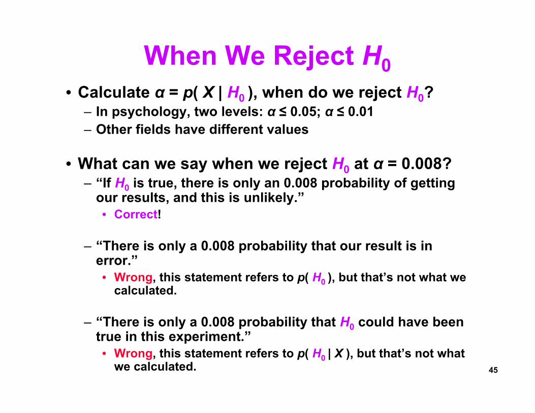
When We Reject H0• Calculate α = p( X | H0 ), when do we reject H0?

– In psychology, two levels: α ≤ 0.05; α ≤ 0.01– Other fields have different values

• What can we say when we reject H0 at α = 0.008?– “If H0 is true, there is only an 0.008 probability of getting

our results, and this is unlikely.”• Correct!

– “There is only a 0.008 probability that our result is in error.”• Wrong, this statement refers to p( H0 ), but that’s not what we

calculated.

– “There is only a 0.008 probability that H0 could have been true in this experiment.”• Wrong, this statement refers to p( H0 | X ), but that’s not what

we calculated.

46

When We Don’t Reject H0• What can we say when we don’t reject H0 at α = 0.445?– “We have proved that H0 is true.”– “Our experiment indicates that H0 is true.”

• Wrong, statisticians agree that hypothesis testing cannot prove H0 is true.

• Statisticians do not agree on what failing to reject H0 means.– Conservative viewpoint (Fisher):

• We must suspend judgment, and cannot say anything about the truth of H0.

– Alternative viewpoint (Neyman & Pearson): • We “accept” H0, and act as if it’s true for now…• But future data may cause us to change our mind


47

Hypothesis Testing Outcomes

• α = p( X | H0 ), so hypothesis testing involves calculating α• Two ways to be right:

– Find a result– Fail to find a result and waste time running an experiment

• Two ways to be wrong:– Type I error: we think we have a result, but we are wrong– Type II error: a result was there, but we missed it

correct(but wasted time)

p = 1 – α

wrongtype I error

p = αH0 true

wrongtype II error

p = β

correcta result!

p = 1 – β = powerH0 falseTrue

state of the world

Don’t reject H0Reject H0

Decision

48

When Do We Really Believe a Result?• When we reject H0, we have a result, but:

– It’s possible we made a type I error– It’s possible our finding is not reliable

• Just an artifact of our particular experiment

• So when do we really believe a result?– Statistical evidence

• α level: (p < .05, p < .01, p < .001)• Power

– Meta-statistical evidence• Plausible explanation of observed phenomena

– Based on theories of human behavior:perceptual, cognitive psychology; control theory, etc.

• Repeated results– Especially by others

49

Hypothesis Testing Means• Empiricism• Experimental Validity• Usability Engineering• Experimental Design• Gathering Data• Describing Data



50

Hypothesis Testing Means• How do we calculate α = p( X | H0 ), when X is a

mean?– Calculation possible for other statistics, but most

common for means

• Answer: we refer to a sampling distribution• We have two conceptual functions:

– Population: unknowable property of the universe– Distribution: analytically defined function,

has been found to match certain population statistics

51

Calculating α = p( X | H0 ) with A Sampling Distribution

• Sampling distributions are analytic functions with area 1• To calculate α = p( X | H0 ) given a distribution, we first

calculate the value D, which comes from an equation of the form:

• α = p( X | H0 ) is equal to:– Probability of seeing a value ≥ | D |– 2 * (area of the distribution to the right of | D |)

• If H0 true, we expect D to be near central peek of distribution• If D far from central peek, we have reason to reject the idea

that H0 is true

( )( )( )( ) , :effect ofty variabili

:effect of size 2 Nsf

XfD =

D?D?

Represents assumptionthat H0 true

52

0

0.1

0.2

0.3

0.4

-4 -3 -2 -1 0 1 2 3 4

A Distribution for Hypothesis Testing Means

• The Standard Normal Distribution (μ = 0, σ = 1)

( )( )

2

2

2

21,; σ

μ

πσσμ

−−

=X

eXN

53

The Central Limit Theorem• Full Statement:

– Given population with (μ, σ2), the sampling distribution of means drawn from this population is distributed (μ, σ2/n), where n is the sample size. As n increases, the sampling distribution of means approaches the normal distribution.

• Implication:– As n increases, distribution of means becomes

normal, regardless of how “non-normal” the population looks.

• How big does n have to be before means look normally distributed?– For very “non-normal” data, n ≈ 30.

54

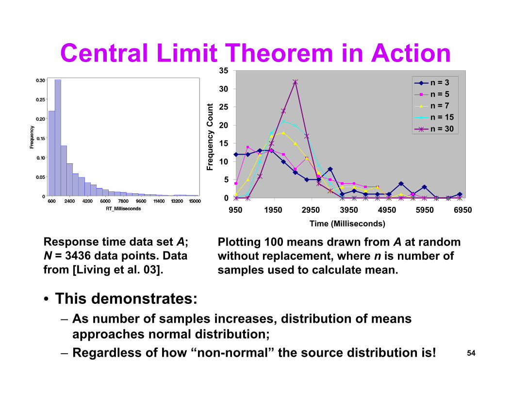
Central Limit Theorem in Action

• This demonstrates: – As number of samples increases, distribution of means

approaches normal distribution;– Regardless of how “non-normal” the source distribution is!

0

5

10

15

20

25

30

35

950 1950 2950 3950 4950 5950 6950Time (Milliseconds)

Freq

uenc

y C

ount

n = 3n = 5n = 7n = 15n = 30

Response time data set A; N = 3436 data points. Data from [Living et al. 03].

Plotting 100 means drawn from A at random without replacement, where n is number of samples used to calculate mean.

55

The t Distribution• In practice, when H0: μc – μd = 0

(two means come from same population), we calculate α = p( X | H0 ) from t distribution, not Z distribution

• Why? Z requires the population parameter σ2, but σ2 almost never known. We estimate σ2 with s2, but s2 biased to underestimate σ2. Thus, t more spread out than Z distribution.

• t distribution parametric: parameter is df (degrees of freedom)


At ∞ df, t distribution same as normal distribution

56

t-Test Example• Null hypothesis H0: μs – μm = 0

– Subjects same speed whether stereo or mono viewing.

• Ran an experiment and collected samples:– 32 subjects, collected 128 samples– ns = 64, Xs = 36.431 sec, ss = 15.954 sec– nm = 64, Xm = 34.449 sec, sm = 13.175 sec

• Look up t(126) = 0.766 in a t-distribution table: 0.445

• Thus, α = p(1.983 sec | H0 ) = 0.445, and we do not reject H0.

Calculation described by [Howell 02], p 202

( ) ( )( )

( ) ( )2

11,766.011,

12622

2

22 −+

−+−==

⎟⎠⎞⎜

⎝⎛ +

−==

ms

mmssp

msp

ms

nnsnsns

nns

XXNsf

Xft

0 0.766

Area of shadedregions: 0.445

- 0.766

t(126) distribution

57

One- and Two-Tailed Tests• t-Test example is a two-tailed test.

– Testing whether two means differ, no preferred direction of difference: H1: μs – μm = d, either μs > μm or μs < μm

– E.g. comparing stereo or mono in VE: either might be faster– Most stat packages return two-tailed results by default

• One-tailed test is performed when preferred direction of difference: H1: μs > μm– E.g. in [Meehan et al. 03], hypothesis is that heart rate &

skin conductance will rise in stressful virtual environment

0 0.766

Area of shadedregions: 0.445

- 0.7660 0.139

Area of shadedregion: 0.445

one-tailed test two-tailed test

58

Power• Empiricism• Experimental Validity• Usability Engineering• Experimental Design• Gathering Data• Describing Data



59

Interpreting α, β, and Power

• If H0 is true:– α is probability we make a

type I error: we think we have a result, but we are wrong

• If H1 is true:– β is probability we make a

type II error: a result was there, but we missed it

– Power is a more common term than β

wasted timep = 1 – α

type I errorp = αH0 true

type II errorp = β

a result!p = 1 – β = powerH0 falseTrue

state of the world

Don’t reject H0Reject H0

Decision

αμ1μ0

H0 H1

β

power =1 – β

60

Increasing Power by Increasing α

• Illustrates α / powertradeoff

• Increasing α:– Increases power– Decreases type II error– Increases type I error

• Decreasing α:– Decreases power– Increases type II error– Decreases type I error

αμ1μ0

H0 H1

β

power

αβ

power

μ1μ0

H0 H1

61

Increasing Power by Measuring a Bigger Effect

• If the effect size is large:– Power increases– Type II error

decreases– α and type I error stay

the same

• Unsurprisingly, large effects are easier to detect than small effects

αμ1μ0

H0 H1

β

power

αμ1μ0

β

power

H0 H1

62

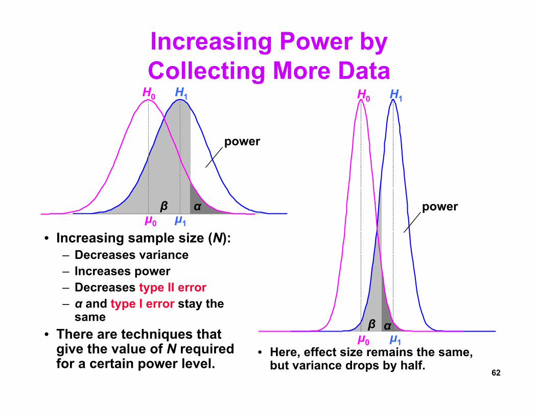
Increasing Power by Collecting More Data

• Increasing sample size (N):– Decreases variance– Increases power– Decreases type II error– α and type I error stay the

same• There are techniques that

give the value of N required for a certain power level.

• Here, effect size remains the same, but variance drops by half.

αμ1μ0

H0 H1

β

power

H0 H1

αμ1μ0

β

power

63

Analysis of Variance and Factorial Experiments

• Empiricism• Experimental Validity• Usability Engineering• Experimental Design• Gathering Data• Describing Data



64

ANOVA: Analysis of Variance• t-test used for comparing two means

– (2 x 1 designs)

• ANOVA used for factorial designs– Comparing multiple levels (n x 1 designs)– Comparing multiple independent variables

(n x m, n x m x p), etc.– Can also compare two levels (2 x 1 designs);

ANOVA can be considered a generalization of a t-Test

• No limit to experimental design size or complexity

• Most widely used statistical test in psychological research

• ANOVA based on the F Distribution; also called an F-Test

65

How ANOVA Works

• Null hypothesis H0: μ1 = μ2 = μ3 = μ4; H1: at least one mean differs• Estimate variance between each group: MSbetween

– Based on the difference between group means– If H0 is true, accurate estimation– If H0 is false, biased estimation: overestimates variance

• Estimate variance within each group: MSwithin– Treats each group separately– Accurate estimation whether H0 is true or false

• Calculate F critical value from ratio: F = MSbetween / MSwithin– If F ≈ 1, then accept H0

– If F >> 1, then reject H0

H0 likelytrue

H0 likelyfalse

66

ANOVA Uses The F Distribution• Calculate α = p( X | H0 ) by looking up F critical value in

F-distribution table• F-distribution parametric: F ( numerator df, denominator df )• α is area to right of F critical value (one-tailed test)• F and t are distributions are related: F ( 1, q ) = t ( q )

From [Saville Wood 91], p 52, and [Devore Peck 86], p 563

67

ANOVA Example• Hypothesis H1:

–Platform (Workbench, Desktop, Cave, or Wall) will affect user navigation time in a virtual environment.

• Null hypothesis H0: μb = μd = μc = μw.–Platform will have no effect on user

navigation time.• Ran 32 subjects, each subject used

each platform, collected 128 data points.

• Reporting in a paper: F( 3, 93 ) = 3.1, p < .05

20

25

30

35

40

45

50

55

60

Workbench Desktop Cave Wall

Platform

Tim

e (s

econ

ds)

± 95% Confidence Intervals

*p < .05129.66779312059.0950Within (P x S)

0.0313.100*401.962531205.8876Between (platform)pFMSdfSSSource

Data from [Swan et al. 03], calculations shown in [Howell 02], p 471

68

Main Effects and Interactions• Main Effect

– The effect of a single independent variable– In previous example, a main effect of platform on user

navigation time: users were slower on the Workbench, relative to other platforms

• Interaction– Two or more variables interact– Often, a 2-way interaction can describe main effects


69

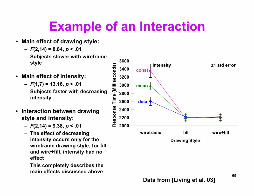
Example of an Interaction• Main effect of drawing style:

– F(2,14) = 8.84, p < .01– Subjects slower with wireframe

style

• Main effect of intensity:– F(1,7) = 13.16, p < .01– Subjects faster with decreasing

intensity

• Interaction between drawing style and intensity:

– F(2,14) = 9.38, p < .01– The effect of decreasing

intensity occurs only for the wireframe drawing style; for fill and wire+fill, intensity had no effect

– This completely describes the main effects discussed above

2000

2200

2400

2600

2800

3000

3200

3400

3600

wireframe fill wire+fill

Drawing Style

Res

pons

e Ti

me

(Mill

isec

onds

)

const

decr

±1 std errorIntensity

mean

Data from [Living et al. 03]

70

Reporting Statistical Results• For parametric tests, give degrees of freedom, critical value,

p value:– F(2,14) = 8.84*, p < .01 (report pre-planned significance value)– t(8) = 4.11, p = .0034 (report exact p value)– F(8,12) = 5.826403, p = 3.4778689e10-3

(too many insignificant digits)

• Give primary trends and findings in graphs– Best guide is [Tufte 83]

• Use graphs / tables to give data, and use text to discuss what the data means– Avoid giving too much data in running text

71

References[Devore Peck 86] J Devore, R Peck, Statistics: The Exploration and Analysis of Data,

West Publishing Co., St. Paul, MN, 1986.[Living et al. 03] MA Livingston, JE Swan II, JL Gabbard, TH Höllerer, D Hix, SJ Julier,

Y Baillot, D Brown, “Resolving Multiple Occluded Layers in Augmented Reality”, The 2nd International Symposium on Mixed and Augmented Reality (ISMAR ’03), October 7–10, 2003, Tokyo, Japan, pages 56–65.

[Howell 02] DC Howell, Statistical Methods for Psychology, 5th edition, Duxbury, Pacific Grove, CA, 2002.

[Meehan et al. 03] M Meehan, S Razzaque, MC Whitton, FP Brooks, Jr., “Effect of Latency on Presence in Stressful Virtual Environments”, Technical Papers, IEEE Virtual Reality 2003, March 22–26, Los Angeles, California: IEEE Computer Society, 2003, pages 141–148.

[Saville Wood 91] DJ Saville, GR Wood, Statistical Methods: The Geometric Approach, Springer-Verlag, New York, NY, 1991.

[Swan et al. 03] JE Swan II, JL Gabbard, D Hix, RS Schulman, KP Kim, “A Comparative Study of User Performance in a Map-Based Virtual Environment”, Technical Papers, IEEE Virtual Reality 2003, March 22–26, Los Angeles, California: IEEE Computer Society, 2003, pages 259–266.

[Tufte 90] ER Tufte, Envisioning Information, Graphics Press, Cheshire, Connecticut, 1990.

[Tufte 83] ER Tufte, The Visual Display of Quantitative Information, Graphics Press, Cheshire, Connecticut, 1983.

72

Contact Information

J. Edward Swan II, Ph.D.The Naval Research Laboratory

Washington, [email protected]

202/404-4984

Conducting Human-Subject Experiments with...

Documents

Transcript of Conducting Human-Subject Experiments with...