Conditions on the elasticity factor of the variance for strong solutions of the option pricing model

IntroductionStrong and weak solutions (Existence and Uniqueness)

Condition for RegularityThe CEV. share price solution

The CEV. option pricing formulaConclusionReferences

Conditions on the elasticity factor of the variance for strongsolutions of the option pricing model

Br. Dennis N. Quispe Sanchez

Dr. Obidio Rubio Mercedes

Universidad Nacional de Trujillo

Br. Dennis N. Quispe Sanchez Dr. Obidio Rubio Mercedes Conditions on the elasticity factor of the variance for strong solutions of the option pricing Model




Outline

1 Introduction

2 Strong and weak solutions (Existence and Uniqueness)

3 Condition for Regularity

4 The CEV. share price solution

5 The CEV. option pricing formula

6 Conclusion

7 References





The main object of this work is the study of the stochastic differential equation(the constant elasticity of variance model, C.E.V.).

dS(t) = µS(t)dt+ σS(t)β2 dW (t) , 0 ≤ t <∞ (1)

donde S = S(t), 0 ≤ t <∞ is a process with continuous sample paths, andµ, σ, β are constants. We analize the cases: β < 2, β = 2 and β > 2.Using theory of stochastic differential equations establish conditions on theparameter β (elasticity factor) in order to the existense and uniqueness of strongsolutions of equation (1), otherwise establish a regularity condition of the possibleweak solutions.Theoretical support for this model for different cases (β < 2, β = 2, β > 2) can befound in Cox [3], Black [2] and Mac Beth [6] respectively.Finally based in Cox [3] and Schroeder [8], we employ consistent notation toobtain the pricing option formula.





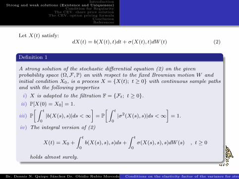
Let X(t) satisfy:dX(t) = b(X(t), t)dt+ σ(X(t), t)dW (t) (2)

Definition 1

A strong solution of the stochastic differential equation (2) on the givenprobability space (Ω,F ,P) an with respect to the fixed Brownian motion W andinitial condition X0, is a process X = X(t); t ≥ 0 with continuous sample pathsand with the following properties

i) X is adapted to the filtration F = Ft; t ≥ 0.ii) P[X(0) = X0] = 1.

iii) P[ ∫ t

0|b(X(s), s)|ds <∞

]= P

[ ∫ t

0|σ2(X(s), s)|ds <∞

]= 1.

iv) The integral version of (2)

X(t) = X0 +

∫ t

0b(X(s), s), s)ds+

∫ t

0σ(X(s), s), s)dW (s) , t ≥ 0

holds almost surely.





Definition 2

A weak solution of equation (2) is a triple (X,W ), (Ω,F ,P), Ft where

i) (Ω,F ,P) is a probability space, and Ft is a filtration of sub σ−fields of Fsatisfying the usual conditions.

ii) X = X(t), Ft, 0 ≤ t <∞ is a continuous, adapted R−valued processW = W (t), Ft, 0 ≤ t <∞ is a 1−dimensional Brownian motion, and

iii), iv) of Definition 1 are satisfied.

Definition 3

We say that uniqueness in the sense of probability law holds for equation (2) if,for any two weak solutions (X,W ), (Ω,F ,P), Ft and (X,W ), (Ω,F ,P), Ft,with the same initial distribution, ie

P[X0 ∈ A] = P[X0 ∈ A] , ∀ A ∈ B(R)

the two processes X, X have the same distribution.





Theorem 1

Suppose that the coefficients b(x, t), σ(x, t) satisfy the global lipschitz and lineargrowth conditions

|b(x, t)− b(y, t)|+ |σ(x, t)− σ(y, t)| ≤ K|x− y|

|σ(x, t)|+ |b(x, t)| ≤ K(1 + |x|)

for every 0 ≤ t <∞, x ∈ R, y ∈ R, where K is a positive constant. On someprobability space (Ω,F ,P), let X0 be a R−valued random variable, independent ofthe Brownian motion W , and with finite second moment.

E[|X0|2] <∞

Then there exist a continuous, adapted process X which is a strong solution ofequation (2) relative to W , with initial condition X0.





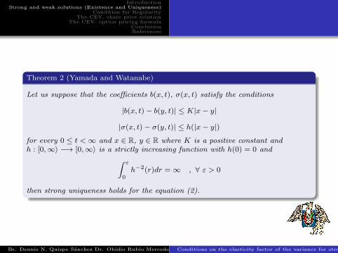
Theorem 2 (Yamada and Watanabe)

Let us suppose that the coefficients b(x, t), σ(x, t) satisfy the conditions

|b(x, t)− b(y, t)| ≤ K|x− y|

|σ(x, t)− σ(y, t)| ≤ h(|x− y|)

for every 0 ≤ t <∞ and x ∈ R, y ∈ R where K is a positive constant andh : [0,∞〉 −→ [0,∞〉 is a strictly increasing function with h(0) = 0 and∫ ε

0h−2(r)dr =∞ , ∀ ε > 0

then strong uniqueness holds for the equation (2).





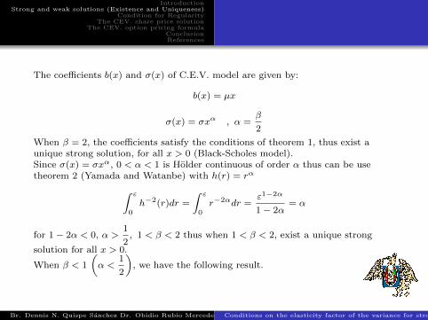
The coefficients b(x) and σ(x) of C.E.V. model are given by:

b(x) = µx

σ(x) = σxα , α =β

2

When β = 2, the coefficients satisfy the conditions of theorem 1, thus exist aunique strong solution, for all x > 0 (Black-Scholes model).Since σ(x) = σxα, 0 < α < 1 is Holder continuous of order α thus can be usetheorem 2 (Yamada and Watanbe) with h(r) = rα∫ ε

0h−2(r)dr =

∫ ε

0r−2αdr =

ε1−2α

1− 2α= α

for 1− 2α < 0, α >1

2, 1 < β < 2 thus when 1 < β < 2, exist a unique strong

solution for all x > 0.

When β < 1

(α <

1

2

), we have the following result.





Theorem 3

Assume that σ−2 is locally integrable at every point in R and that conditions:

i) σ2(x) > 0

ii) ∀ x ∈ R ∃ ε > 0 such that ∫ x+ε

x−ε

b(y)

σ2(y)dy <∞

hold. Then for every initial distribution, the equation (2) has a weak solutionand this solution is unique in the sense of probability law (definition 3)

If σ(x) = σxα with α <1

2, the conditions of theorem are satisfied because∫ x+ε

x−εσ−2(y)dy =

1

σ2

[(x+ ε)1−2α − (x− ε)1−2α

1− 2α

]<∞⇐⇒ 1− 2α > 0

and ∫ x+ε

x−ε

b(y)

σ2(y)dy =

µ

σ2

[(x+ ε)2−2α − (x− ε)2−2α

2− 2α

]<∞ for α <

1

2





Definition 4

Suppose that whenever (X,W ), (Ω,F ,P), Ft and (X,W ), (Ω,F ,P), Ft, areweak solutions to (2) with common Brownian motion W (relative to possiblydifferent filtrations) on a common probability space (Ω,F ,P) and with commoninitial value, ie P[X0 = X0] = 1, the two processes X and X are indistinguishable:P[X(t) = X(t); ∀ 0 ≤ t <∞] = 1 we say then that pathwise uniqueness holds forequation (2).

Yanada and Watanbe shows that pathwise uniqueness implies uniqueness in thesense of probability law, this result has the remarkable consequence

WEAK EXISTENCE + PATHWISE UNIQUENESS = STRONG EXISTENCE





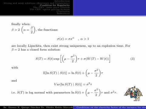
finally when:

β > 2

(α =

β

2

), the functions:

σ(x) = σxα , α > 1

are locally Lipschitz, then exist strong uniqueness, up to an explosion time. Forβ = 2 has a closed form solution:

S(T ) = S(t) exp

[(µ−

σ2

2

)τ + σ(W (T )−W (t))

](3)

with

E[lnS(T ) | S(t)] = lnS(t) +

(µ−

σ2

2

)τ

andV ar[lnS(T ) | S(t)] = σ2τ

i.e. S(T ) is log normal with parameters lnS(t) +

(µ−

σ2

2

)τ and σ2τ .





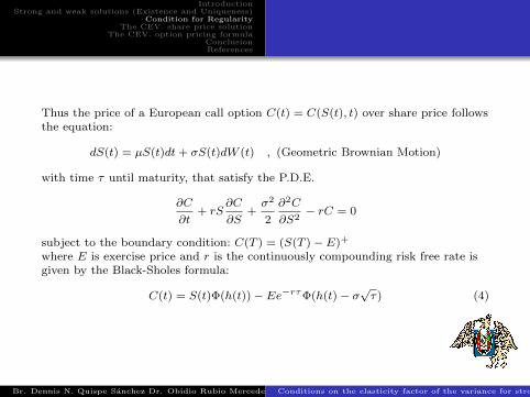
Thus the price of a European call option C(t) = C(S(t), t) over share price followsthe equation:

dS(t) = µS(t)dt+ σS(t)dW (t) , (Geometric Brownian Motion)

with time τ until maturity, that satisfy the P.D.E.

∂C

∂t+ rS

∂C

∂S+σ2

2

∂2C

∂S2− rC = 0

subject to the boundary condition: C(T ) = (S(T )− E)+

where E is exercise price and r is the continuously compounding risk free rate isgiven by the Black-Sholes formula:

C(t) = S(t)Φ(h(t))− Ee−rτΦ(h(t)− σ√τ) (4)





where

h(t) =lnS(t)− lnK + (r + σ2

2)τ

σ√τ

and Φ(x) =

∫ x

−∞φ(z)dz is the standard normal cumulative distribution function

and φ(z) is the standard normal probability density function.But for β < 2 the computation of the exact solution is problematic, MarkSchroeder [8] expresses the constant elasticity of variance option pricing formula interms of the noncentral chi-square distribution. This allow the the application ofwell-know approximation formulas and the derivation of a whole class of closedform solutions.Emanuel and Mac Beth [6] derive a formula for β > 2.





Unlike the Black-Scholes case, for the general CEV model it is not possible toderive a form for S(T) similar to the one we saw in equation (3), the Kolmogorovequations can be used in this context.

Theorem 4

Suppose that b(x, t) and σ(x, t) satisfy the conditions of theorems 1, 2, 3 such thatX(t) is a solution of the S.D.E.

dX(t) = b(X, t)dt+ σ(X, t)dW (t)

with initial condition X(t0) = x0, where σ(x, t) =√a(x, t). Then X(t) has a

transition probability density P (x0, t0;x, t) which satisfies the Kolmogorovequations:

∂p

∂t=

1

2

∂2

∂x2(a(x, t)p)−

∂

∂x(b(x, t)p) (FORWARD) (4.1)

−∂p

∂t0=

1

2a(x0, t0)

∂2p

∂x20

+ b(x0, t0)∂p

∂x0(BACKWARD) (4.2)





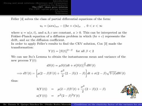
Feller [4] solves the class of partial differential equations of the form:

ut = (axu)xx − ((bx+ c)u)x , 0 < x <∞

where u = u(x, t), and a, b, c are constant, a > 0. This can be interpreted as theFokker-Planck equation of a diffusion problem in which (bx+ c) represents thedrift, and ax the diffusion coefficient.In order to apply Feller’s results to find the CEV solution, Cox [3] made thetransformation:

Y (t) = [S(t)]2−β for all β < 2

We can use Ito’s Lemma to obtain the instantaneous mean and variance of thenew process Y (t):

dS(t) = µS(t)dt+ σ[S(t)]β2 dW (t)

=⇒ dY (t) =

[µ(2− β)Y (t) +

σ2

2(2− β)(1− β)

]dt+ σ(2− β)

√Y (t)dW (t)

thus:

b(Y (t)) = µ(2− β)Y (t) +σ2

2(2− β)(1− β)

a(Y (t)) = σ2(2− β)2Y (t)





The transition density f = fY (T )|Y (t)(y, τ) will satisfy the forward Kolmogorovequation (Theorem 4)

1

2a(Y (t))

∂2f

∂Y (t)2+ b(Y (t))

∂f

∂Y (t)= −

∂f

∂t

which is of the form specified by Feller [4] with:

a =1

2σ2(2− β) , b = µ(2− β) , c =

σ2

2(2− β)(1− β)

This function is given by Feller [4] in his lemma 9, as

fY (T )|Y (t)(y, τ) =b

a(ebτ − 1)exp

(−b(y + Y (t)ebτ )

a(ebτ − 1)

)·(ye−bτ

Y (t)

) c−a2a ·I1− c

a

(2b(e−bτyY (t))1/2

a(1− e−bτ )

)where Iν(z) is the modified Bessel function of the firts kind of order ν

Iν(z) =∞∑n=0

( z2

)2n−ν

n!Γ(n+ ν + 1)





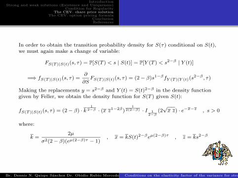
In order to obtain the transition probability density for S(τ) conditional on S(t),we must again make a change of variable:

FS(T )|S(t)(s, τ) = P[S(T ) < s | S(t)] = P[Y (T ) < s2−β | Y (t)]

=⇒ fS(T )|S(t)(s, τ) =∂

∂SFS(T )|S(t)(s, τ) = (2− β)s1−βfY (T )|Y (t)(s

2−β , τ)

Making the replacements y = s2−β and Y (t) = S(t)2−β in the density functiongiven by Feller, we obtain the density function for S(T ) given S(t):

fS(T )|S(t)(s, τ) = (2− β) · k1

2−β · (x z1−2β)1

2(2−β) · I 12−β

(2√x z) · e−x−z , s > 0

where:

k =2µ

σ2(2− β)(eµ(2−β)τ − 1), x = kS(t)2−βeµ(2−β)τ , z = ks2−β





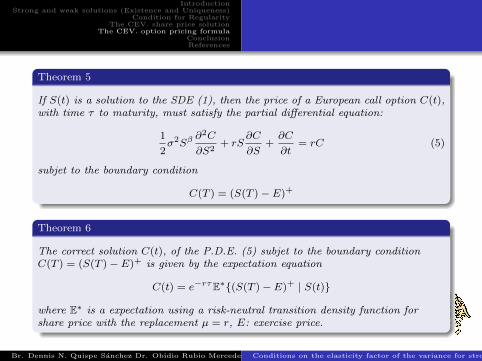
Theorem 5

If S(t) is a solution to the SDE (1), then the price of a European call option C(t),with time τ to maturity, must satisfy the partial differential equation:

1

2σ2Sβ

∂2C

∂S2+ rS

∂C

∂S+∂C

∂t= rC (5)

subjet to the boundary condition

C(T ) = (S(T )− E)+

Theorem 6

The correct solution C(t), of the P.D.E. (5) subjet to the boundary conditionC(T ) = (S(T )− E)+ is given by the expectation equation

C(t) = e−rτE∗(S(T )− E)+ | S(t)

where E∗ is a expectation using a risk-neutral transition density function forshare price with the replacement µ = r, E: exercise price.





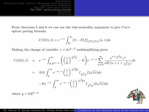
From theorems 5 and 6 we can use the risk-neutrality argument to give Cox’soption pricing formula:

C(S(t), t) = e−rτ∫ ∞K

(S − E)f∗S(T )|S(t)(s, τ)ds

Making the change of variable: z = ks2−β andsimplifying gives

C(S(t), t) = e−rτ∫ ∞KE2−β

((z

k

) 12−β− E

)e−x−z

∞∑n=0

xn+ 1

2−β zn

n!Γ(n+ 1 + 12−β )

dz

= S(t)

∫ ∞y

e−x−z(z

x

) 14−2β

I 12−β

(2√xz)dz

−Ee−rτ∫ ∞y

e−x−z(x

z

) 14−2β

I 12−β

(2√xz)dz

where y = kE2−β





Since:

e−rτ(x

k

) 12−β

= e−rτ (S(t)2−βer(2−β)τ )1

2−β = S(t)

Schroder recognisees that the integrands are both non-central Chi-square densityfunctions. See Johnson and Kotz [ ] they introduce the non-central Chi-squaredistribution:The density function of such a variable is given as:

P (y, ν, λ) =1

2

(y

λ

) 14

(ν−2)

exp

−

1

2(y + λ)

· I 1

2(ν−2)(

√λy)

with ν degrees of freedom, and non centrality parameter λ.

Theorem 7

The CEV option price may be written

C(t) = S(t)

∫ ∞y

2P (2z, 2 +2

2− β, 2x)dz − Ee−rτ

∫ ∞y

2P (2x, 2 +2

2− β, 2z)dz

where y = kE2−β





Note that as written, reither of the integrals are non central Chi square survivorfunctions at y.Result 1: ∫ ∞

y2P (2x, 2ν + 2, 2z)dz = 1−

∫ ∞x

2P (2z, 2ν, 2y)dz

Theorem 8 (Schroder’s Option Pricing Formula)

The form of the CEV option price given by Schroeder (1989) is

C(t) = S(t)Q(2y, 2 +2

2− β, 2x)− Ee−rτ

(1−Q(2x,

2

2− β, 2y)

)where Q(y, ν, λ) is the survivor function at y for a non central Chi-square randomvariable with ν degrees of freedom and non centrality parameter λ.

Proof. The proof this result follows from Theorem 7 and result 1





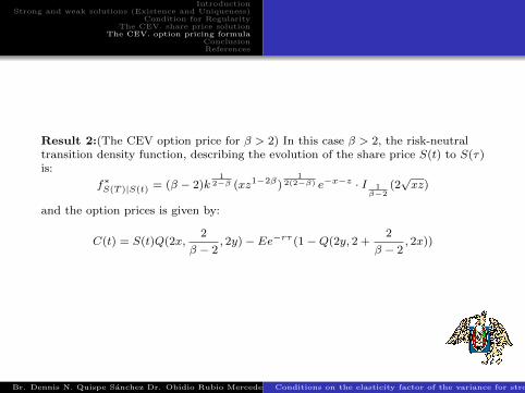
Result 2:(The CEV option price for β > 2) In this case β > 2, the risk-neutraltransition density function, describing the evolution of the share price S(t) to S(τ)is:

f∗S(T )|S(t) = (β − 2)k1

2−β (xz1−2β)1

2(2−β) e−x−z · I 1β−2

(2√xz)

and the option prices is given by:

C(t) = S(t)Q(2x,2

β − 2, 2y)− Ee−rτ (1−Q(2y, 2 +

2

β − 2, 2x))





Conclusion

For all value of β (elasticity factor) the constant elasticity of variance optionpricing model possess a strong solution for each one of the cases:If β = 2 the Black-Scholes Option Pricing Formula is given for

C(t) = S(t)Φ(h(t))− Ee−rτΦ(h(t)− σ√τ)

If β < 2 the Schoeder Option Pricing Formula is given for

C(t) = S(t)Q(2y, 2 +2

2− β, 2x)− Ee−rτ (1−Q(2x,

2

2− β, 2y))

If β > 2 the MacBeth Option Pricing Formula is given for

C(t) = S(t)Q(2x,2

β − 2, 2y)− Ee−rτ (1−Q(2y, 2 +

2

β − 2, 2x))





References

Beckers S., “The Constant Elasticity of Variance Model and Its Implications for Option

Pricing”, Journal of Finance Vol 35, 1980.

Black F. ,Scholes M., “The Pricing of Option and Corporate Liabilities”, Journal of

Political Economics Vol 81, 1973.

Cox J., “Notes on Option Pricing I: Constant Elasticity of Variance Diffusions”, Stanford

University, Graduate School Business,1975.

Feller W., “Two Singular Diffusions Problems”, Two Singular Diffusions Problems.

Karatzas I., “Brownian Motion and Stochastic Calculus”, Springer Verlag ,1990.

MacBeth J., “Further Results on the Constant Elasticity of Variance Call Option Pricing

Model”, Journal of Financial and Quantitative Analysis, Vol 17, 1982.

Sankaran M., “. On the Non Central Chi square Distribution”, Biometrika ,Vol 46, 1960.

Schoeder M., “Computing the Constant Elasticity of Variance Option Pricing Model ”,

Journal of Finance, Vol 44, 1990.


Conditions on the elasticity factor of the variance for strong solutions of the option pricing model

Education

Transcript of Conditions on the elasticity factor of the variance for strong solutions of the option pricing model