CONDITIONING DISCRETE FRACTURE NETWORK MODELS OF GROUNDWATER FLOW

INTERNATIONAL JOURNAL OF c© 2011 Institute for ScientificNUMERICAL ANALYSIS AND MODELING Computing and InformationVolume 8, Number 4, Pages 543–565

CONDITIONING DISCRETE FRACTURE NETWORK MODELS

OF GROUNDWATER FLOW

K. CLIFFE, D. HOLTON, P. HOUSTON, C. JACKSON, S. JOYCE, AND A. MILNE

Abstract. Many geological formations consist of crystalline rock that have

very low matrix permeability but allow flow through an interconnected net-

work of fractures. Understanding the flow of groundwater through such rocks

is important in considering disposal of radioactive waste in underground reposi-

tories. A specific area of interest is the conditioning of fracture transmissivities

on measured values of pressure in these formations. While there are exist-

ing methods to condition transmissivity fields on transmissivity, pressure and

flow measurements for a continuous porous medium, considerably less work has

been devoted to conditioning discrete fracture networks. This article presents

two new methods for conditioning fracture transmissivities on measured pres-

sures in a discrete fracture network. The first approach adopts a linear ap-

proximation when fracture transmissivities are mildly heterogeneous, while the

minimisation of a suitable objective function is undertaken when fracture trans-

missivities are highly heterogeneous. The second conditioning algorithm is a

Bayesian method that finds a maximum a posteriori (MAP) estimator which

maximises the posterior distribution defined by Bayes’ theorem using informa-

tion from the prior distribution of fracture transmissivities and observations in

the form of measured pressures. The conditioning methods are tested on two

separate, large scale test cases that model a potential site for radioactive waste

disposal. Results from these test cases are shown and comparisons between the

two conditioning methods are made.

Key Words. Conditioning, Groundwater Flow, Discrete Fracture Network,

Finite Element Methods.

1. Introduction

Many geological formations consist of crystalline rock that have very low matrixpermeability but allow flow through an interconnected network of fractures. Un-derstanding the flow of groundwater through such rocks is important in consideringdisposal of radioactive waste in underground repositories. In our work it is assumedthat there is no interaction between groundwater flow (and the pollutants it maycarry) in the fractures and the surrounding rock matrix; this setting is known as adiscrete fracture network (DFN). A DFN is characterised by the properties of thefractures, namely, the density of the fractures, their size, orientation and transmis-sivity. The transmissivity of a fracture is defined as the rate of groundwater flow perunit pressure gradient. It thus gives a measure of the ease with which groundwatercan pass through a material (a fracture in our case). In our work the fractures aremodelled such that the fracture walls are represented as two parallel plates with

Received by the editors February 7, 2011.2000 Mathematics Subject Classification. 35L60, 35Q35, 76B15, 76B65.

543

544 K. CLIFFE, D. HOLTON, P. HOUSTON, C. JACKSON, S. JOYCE, AND A. MILNE

groundwater flowing between them. In this setting, the fracture transmissivity isproportional to the cube of the fracture aperture (width between the fracture walls)[21], and both the aperture and transmissivity are constant over the fracture. In aproblem of practical relevance, there are generally too many fractures for all of theirproperties to be measured. To remedy this problem when numerically modelling aDFN, a stochastic approach can be exploited; here distributions of fracture prop-erties (aperture, length, orientation, location) are inferred from field measurementsand are subject to uncertainty [12, 17]. Realisations of fractures can be generatedin a given domain with fracture properties (aperture, length, orientation, location)sampled from distributions consistent with observed measurements. Fractures withknown properties can also be included deterministically in a model of this type.This paper develops two numerical methods in a DFN setting to condition fracturetransmissivities on measured values of the pressure available from test site data.The groundwater flow equation [1] can be used to calculate the pressure in a frac-ture. DFNs are modelled numerically with suitable boundary conditions at bothfracture intersections and the domain boundaries [8]. Our work exploits a finiteelement approach to modelling groundwater flow in a DFN. Alternative numericalmethods for solving flow in a DFN are discussed in Jing [10].

The problem considered in this article can be summarised in a continuous setting(before discretisation of the domain) as follows: determine T such that

‖P (XM )−PM‖ = min!,

under the constraint,

∇ · (T∇P ) = 0 in Ω,

subject to appropriate boundary conditions. Here, T is a vector of fracture trans-missivities (containing hundreds or thousands of fracture transmissivities), PM ,M ≥ 1, is a vector of measured pressures that are to be matched, XM , M ≥ 1,denotes the locations of the measurement points, P is the pressure, Ω is the do-main of the fracture network and ‖ · ‖ denotes an appropriate norm. Boundaryconditions are imposed both on the boundaries of the problem domain Ω, as well asat fracture intersections. Generally, there are far less pressure measurements thanfracture transmissivities.

When studying DFNs it is common to use more than one realisation of theDFN due to uncertainties in the fracture properties. In this setting, the geometryof the fractures is sampled from various distributions; thus each realisation willhave different fracture geometry. Calibration is the process of modifying inputparameters to a model until the output from the model matches observed data.Each realisation should be calibrated using as much available data as possible.In our work the model parameters are the fracture transmissivities and they areconditioned on measured pressures.

While there are existing methods to condition transmissivity fields on transmis-sivity, pressure and flow measurements for a continuous porous medium [9, 19, 20],there is considerably less work within the literature on conditioning DFNs. Anexception is the recent work by Frampton and Cvetkovic [5] who condition the pa-rameters of a fracture transmissivity distribution in a DFN setting, but they do notcondition fracture transmissivities directly. Conditioning fracture transmissivitieson pressure or flow values is a complex problem because the measured pressuresare dependent on all the fracture transmissivities in the DFN.

In this article, we present two new methods for conditioning fracture transmissiv-ities in a DFN on measured pressure values. Both methods consider one realisation,

CONDITIONING DISCRETE FRACTURE NETWORK MODELS 545

where the geometry of the DFN is assumed fixed. In particular, only fracture trans-missivities are adjusted to fit measured pressures, while keeping the position andorientation of each fracture fixed. The first method adopts a linear approxima-tion when fracture transmissivities are mildly heterogeneous and generalises thisapproach to the minimisation of an appropriate objective function when fracturetransmissivities are highly heterogeneous. This method is based on a generalisationof previous work undertaken on conditioning transmissivity values in a continuousporous medium [3] and shares some of the techniques used in inverse problems inhydrology for a continuous porous medium [9, 14, 15, 19, 20].

The second method we develop is a Bayesian conditioning method similar to thework developed in a continuous porous medium setting in the articles [2, 11]. Stuart[18] gives a concise review of the Bayesian setting used in inverse methods for PDEs.Here, Bayes’ theorem is used to give an expression of proportionality for the pos-terior distribution of fracture log transmissivities in terms of the prior distributionand the data available through pressure measurements. The fracture transmissivi-ties are assumed to be normally distributed with a given mean and covariance, andthe measured pressures are assumed to be normally distributed values, each witha given error. From the expression of proportionality for the posterior distributionof fracture transmissivities, the modes of the posterior distribution (the points ofhighest likelihood for the fracture transmissivities given the measured pressures)are computed numerically.

The paper is structured as follows. In Section 2 we introduce the PDE modelused to determine the pressure in a fracture network, together with details of theapplication of the finite element method to the DFN. Section 3 introduces thetwo conditioning methods, while section 4 describes the two test cases that will beconsidered in this article. Results obtained from both the conditioning methods arepresented in section 5. Here, both algorithms are implemented in the existing finiteelement code ConnectFlow [8] developed and marketed by Serco, which numericallymodels groundwater flow in a DFN using a finite element approach. Finally, wesummarise the work presented in this article and draw some conclusions in Section 6.

2. Finite Element Treatment of Intersecting Fractures

In this section we outline the finite element (FE) method implemented withinConnectFlow to discretise a DFN in order to compute the residual pressure onfracture intersections. The FE method employed here is based on a standard FEdiscretisation of each fracture, together with a static condensation technique whicheliminates the internal degrees of freedom on each fracture, thereby leading to aglobal system of equations for the unknowns defined on the fracture intersectionsonly. In order to present this algorithm in the simplest possible setting, here weshall confine ourselves to the case of two intersecting fractures. The extension of theFE method to a large scale DFN follows analogously; for further details, we refer toMilne [13] and Hartley [8]. With this in mind, we assume that the problem domainΩ ⊂ R

3 is partitioned into two two–dimensional planes f1 and f2 (which representthe fractures) with boundaries ∂f1 and ∂f2, respectively. Here, we assume that thefractures f1 and f2 do not overlap, in the sense that their orientations in R

3 are notidentical, but that the fractures do intersect one another along a one–dimensionalline Γ := f1 ∩ f2. The residual pressure

(1) P = PG + ρg (z − z0) ,

is to be calculated across f1 and f2, where PG is the groundwater pressure, ρ isthe groundwater density, g is gravitational acceleration, z is the elevation and z0


is a reference elevation. Defining Tf = Tf/(ρg), the steady state groundwater flowequation is given by: find P such that

∇ ·(

Tfi∇P)

= 0, in fi, i = 1, 2,(2)

P = PD, on ∂fi, i = 1, 2,(3)

where the transmissivities Tf1 and Tf2 are assumed constant on f1 and f2, re-spectively, and ∇ denotes the two dimensional gradient operator. At the fractureintersection Γ, the following conditions hold:

(1) The groundwater pressure is continuous between intersecting fractures; i.e.,P |f1∩Γ = P |f2∩Γ.

(2) Groundwater is conserved at the intersection, so that groundwater whichflows out of one fracture flows into the other fracture and there is no buildup of groundwater at the intersection. In the continuous setting, this iswritten as Qf1 := Tf1∇Pf1 = Qf2 := Tf2∇Pf2 , where Qf1 and Qf2 are theflows coming from f1 and f2, respectively, and Pf1 and Pf2 are the pressuresdefined on f1 and f2, respectively.

We now outline the FE method employed to discretise (2), (3), together with theabove intersection conditions. To this end, we assume that the fractures fi, i = 1, 2,can be subdivided into shape-regular meshes Tfi = κfi, i = 1, 2, respectively,consisting of triangular elements κfi , i = 1, 2. Moreover, we define Nfi , i = 1, 2, todenote the set of vertices contained in the meshes Tfi = κfi, i = 1, 2, respectively.In the following, we shall refer to these sets as the sets of so–called local nodes.Further, we write nfi to denote the cardinality of Nfi , i = 1, 2.

The fracture intersection Γ is subdivided into a set NΓ of so–called global nodes;here, we write nΓ to denote the cardinality of the set NΓ. For simplicity of pre-sentation, we assume that each global node contained in the set NΓ correspondsto a local node on f1 and f2. That is, we may define the set of global nodes asNΓ := Nf1 ∩ Nf2 . In general, this condition is rather restrictive, since it requiresTf1 and Tf2 to match on Γ. We emphasise that this constraint is only imposed forsimplicity of presentation; for the case of the more general setting, see [13]. Withthis notation, we introduce the finite element spaces

Vfi = v ∈ H10 (fi) : v|κfi

∈ P1(κfi), κfi ∈ Tfi, i = 1, 2,

where P1(κfi) denotes the set of linear polynomials on κfi , i = 1, 2.For each global node I, I = 1, ..., nΓ, a corresponding global basis function ΨI is

calculated over the problem domain Ω. With this in mind, we denote ΨfiI , i = 1, 2,

to be the restriction of ΨI over fi, i = 1, 2, respectively, such that ΨI = Ψf1I +Ψf2

I ,

where ΨfiI ∈ Vfi , i = 1, 2.

On each fracture, ΨI is calculated as the FE solution to the steady state ground-water flow equation (2) with P replaced by ΨI , subject to the boundary conditions:

ΨI = 1 at global node I and ΨI = 0, otherwise. Therefore, the contributions Ψf1I

and Ψf2I to the global basis function ΨI corresponding to the global node I are

calculated by solving the linear systems: find ΨfiI ∈ Vfi , i = 1, 2, such that

(4)

∫

fi

Tfi∇ΨfiI · ∇vfidx = 0 ∀vfi ∈ Vfi ,

subject to the boundary conditions: ΨfiI = 1, i = 1, 2, at global node I and Ψfi

I = 0,i = 1, 2, at all other global nodes on Γ.


The FE space VΓ consisting of the global basis functions may now be defined as

VΓ = span ΨInΓ

I=1 .

In order to take into account the Dirichlet boundary conditions, it is necessaryto calculate a (boundary) contribution ΨI,D to the global basis function ΨI , I =

1, . . . , nΓ. To this end, we define the contributions Ψf1I,D on f1 and Ψf2

I,D on f2 to

ΨI,D as follows: find ΨfiI,D ∈ PD + Vfi , i = 1, 2, such that

(5)

∫

fi

Tfi∇ΨfiI,D · ∇vfidx = 0 ∀vfi ∈ Vfi ,

subject to the (additional) boundary condition ΨfiI,D = 0 on Γ, i = 1, 2.

The flow QI at a global node I, I = 1, ..., nΓ, from a fracture f = f1, f2, iscalculated as follows:

(6) QI =

∫

f

∇ΨI ·(

Tf∇Ph

)

dx ∀ΨI ∈ VΓ,

where Ph is defined by

(7) Ph =

nΓ∑

J=1

(ΨJ,D +ΨJPΓJ) .

Here, PΓJdenotes the value of the pressure at the Jth global node. The pressure PΓ

at the fracture intersection Γ can now be calculated by enforcing the condition thatflow is conserved at the fracture intersection. Thereby, employing (6), we deducethat

(8)

∫

f1

∇Ψf1I ·(

Tf1∇Ph

)

dx+

∫

f2

∇Ψf2I ·(

Tf2∇Ph

)

dx = 0, I = 1, ..., nΓ.

Inserting (7) into (8) givesnΓ∑

J=1

(

Tf1

∫

f1

∇Ψf1I · ∇Ψf1

J,Ddx+ Tf1PΓJ

∫

f1

∇Ψf1I · ∇Ψf1

J dx

)

+

nΓ∑

J=1

(

Tf2

∫

f2

∇Ψf2I · ∇Ψf2

J,Ddx+ Tf2PΓJ

∫

f2

∇Ψf2I · ∇Ψf2

J dx

)

= 0,

(9)

for I = 1, ..., nΓ. Introducing the notation

(10) AIJ = Tf1

∫

f1

∇Ψf1I · ∇Ψf1

J dx+ Tf2

∫

f2

∇Ψf2I · ∇Ψf2

J dx

for I, J = 1, ..., nΓ, and

(11) BI = −Tf1

nΓ∑

J=1

∫

f1

∇Ψf1I · ∇Ψf1

J,Ddx− Tf2

nΓ∑

J=1

∫

f2

∇Ψf2I · ∇Ψf2

J,Ddx,

for I = 1, ..., nΓ, the matrix system corresponding to (9) may be written in thefollowing form

(12)

A11 · · · AnΓ1

· · · · · · · · ·A1nΓ

· · · AnΓnΓ

PΓ1

· · ·PΓnΓ

=

B1

· · ·BnΓ

.

The matrix system (12) may now be inverted in order to compute PΓ; thereby, sub-stituting PΓ into (7), the pressure over the two fractures f1 and f2 can subsequentlybe calculated. The overall computational implementation is now summarised in Al-gorithm 2.1 below.


Algorithm 2.1. FE method on a DFN.

(1) Construct finite element meshes Tfi = κfi, i = 1, 2, over each fracturefi, i = 1, 2, in the DFN, respectively.

(2) Discretise the fracture intersection Γ into nΓ global nodes belonging to theset NΓ, such that NΓ = Nf1 ∩Nf2 .

(3) DO I = 1, 2, . . . , nΓ

Compute ΨfiI and Ψfi

I,D using (4) and (5), respectively, i = 1, 2.END DO

(4) Calculate AIJ and BJ defined in (10) and (11), respectively, I, J = 1, . . . , nΓ.(5) Calculate PΓI

, I = 1, .., nΓ, by solving the matrix system (12).(6) Calculate the pressure across the fracture network using the approximation

Ph =∑nΓ

J=1 (ΨJ,D +ΨJPΓJ) .

The FE method outlined in this section is equivalent to applying a standardFE method on the entire fracture network, under the assumption that the globalnodes present on a given fracture intersection correspond to local nodes on bothof the intersecting fractures. The advantage of the proposed FE approach over thestandard FE method is two–fold: firstly, the FE method outlined in this sectiondoes not require the assembly and inversion of a global stiffness matrix; insteadonly local problems on each individual fracture need to be computed, together withthe inversion of the linear system (12). Secondly, the number of global nodes can bereduced by performing a suitable coarsening algorithm at the fracture intersections.In large scale DFNs, such as the ones considered in this article, this approach cangreatly reduce the computational work needed to solve the underlying groundwaterflow problem; see [8, 13] for further details.

3. Conditioning Methods

In this section we develop two numerical methods to condition fracture trans-missivities in a DFN on measured pressure values: the so-called Basis Vector Con-ditioning Method and the Bayesian Conditioning Method. For ease of notation,from hereon we shall refer to the residual pressure as defined in (1) as simply the‘pressure’.

The general problem setting is the following: we suppose that we are given a(deterministically defined) DFN consisting of n, n ≥ 1, fractures, each with an

initial transmissivity Tfi , i = 1, . . . , n. Moreover, we assume that field data hasbeen supplied which provides a set of m measurement points Mi

mj=1 at which

the pressure has been evaluated. We collect these measured pressure values in thevector PM . Once the finite element approximation Ph to the analytical solutionP has been computed, based on employing Algorithm 2.1, we may now evaluatePh at the corresponding measurement points. The aim of this section is then todevelop appropriate conditioning algorithms which are capable of adjusting thetransmissivity field Tfi , i = 1, . . . , n, so that the error ‖PM −Ph,M‖2 is minimised,where ‖ · ‖2 denotes the standard ℓ2–norm and Ph,M = (Ph(M1), . . . , Ph(Mm))⊤.

3.1. Basis Vector Conditioning Method. The material in this section is basedon a conditioning method proposed by Cliffe and Jackson [3, 4], where an isotropictransmissivity field was conditioned on pressure measurements in a continuousporous medium. In this section, we extend this technique so that it is applica-ble to a DFN.

Given a DFN consisting of n fractures, with corresponding transmissivities Tfi ,i = 1, . . . , n, we define the vector X = (X1, . . . , Xn)

⊤ to be equal to the values


of the logarithm of the fracture transmissivities; more precisely, Xi = log10 Tfi ,i = 1, . . . , n. The reason why we condition on the log transmissivities instead ofdirectly on the transmissivities themselves, is that it ensures that the correspond-ing conditioned transmissivities are always positive. It can be shown, see [3], forexample, that for the case of small variability in fracture transmissivities and smalldeviations of the pressure from the mean pressure field, the conditioned realisationsXC of X are given by adding the product of a suitable set of basis vectors W andthe vector of coefficients δP to the unconditioned fracture log transmissivities XU ,i.e.,

XC = XU +W δP ,

where the coefficients in δP are the difference between the measured pressuresPM and the calculated pressure Ph computed at the m measurement points, i.e.,δP = PM −Ph,M . The matrix W, which contains the m basis vectors associatedwith each of the measurement points, can be obtained by solving the system

(13) (LCL⊤)W⊤ = LC ,

cf. [3]. The matrix L is known as the sensitivity matrix, while the covariancematrix C represents the correlation of the fracture transmissivities in the DFN. Itis assumed that the sensitivity matrix L contains pressure measurements only; itrepresents the linear relationship between the values of X on the n fractures and them measured values of pressure for small variability and small deviations of pressurefrom the mean pressure field. The entries of L = Lij, i = 1, . . . ,m, j = 1, . . . , n,are thus defined as

(14) Lij =∂PB(Mi)

∂Xj

, i = 1, . . . ,m, j = 1, . . . , n,

where PB(Mi), i = 1, . . . ,m, is the computed pressure at a borehole evaluated atthe ith measurement point Mi. It is defined as

(15) PB(Mi) = Ph(Mi) +Q(Mi)

Tf,Miκ,

where Q(Mi) is the flow produced from pumping the borehole at Mi, i = 1, . . . ,m,

Tf,Miis the transmissivity of the fracture at the measurement point, and κ is a

geometrical constant dependent on the FE discretisation used. Full details on thederivation of κ can be found in Milne [13]. The consequence G = (G1, . . . , Gm)⊤ isalso defined at each of the m measurement points to be the difference between thecalculated borehole pressure and the measured pressure PM , i.e., defining PB =(PB(M1), . . . , PB(Mm))⊤, we have

(16) G(Ph,X) = PB −PM .

There are two terms needed to calculate the entries in the sensitivity matrix (14)for the case of a DFN; indeed, for a fracture fj, 1 ≤ j ≤ n, we have that

(17) Lij =

∫

fj

1

ρg

∂Tfj

∂Xj

∇θ · ∇Phdx+∂

∂Xj

(

Q(Mi)

Tf,Miκ

)

, j = 1, ..., n.

Here, the first term on the right-hand side of (17) may be rewritten as

(18)

∫

fj

1

ρg

∂Tfj

∂Xj

∇θ · ∇Phdx =

∫

fj

Tfj loge 10

ρg∇θ · ∇Phdx ,

where ∇Ph is the gradient of the pressure on the fracture, fj , j = 1, . . . , n, ρ is thegroundwater density, g is the gravitational acceleration and ∇θ is the gradient of


an associated adjoint solution on the fracture. The adjoint solution is derived inMilne [13]; it is defined at global nodes as follows

(

θ⊤)

ir=

∂Gi

∂PΓr

(

∂Φs

∂PΓr

)−1

, i = 1, . . . ,m, r, s = 1, . . . , nΓ,

where nΓ is the number of global nodes in the DFN at which the pressure PΓ ona fracture intersection is calculated and Φs represents the finite element equationsat the fracture intersections, i.e.,

Φs :=

A11 · · · AnΓ1

· · · · · · · · ·A1nΓ

· · · AnΓnΓ

PΓ1

· · ·PΓnΓ

−

B1

· · ·BnΓ

= 0,

cf. (12). The adjoint solution is then calculated across the fracture network in asimilar manner to the pressure (7). The second term on the right-hand side of (17)

is calculated by differentiating (15) with respect to Xj = log10 Tfj , j = 1, . . . , n, forthe single fracture it corresponds to, i.e.,

(19)∂

∂Xj

(

Q(Mi)

Tf,Miκ

)

= −Q(Mi)δij log10 e

Tfjκ,

where δij denotes the Kronecker delta function. The integral in (18) can be calcu-lated using a numerical quadrature technique while (19) is easily evaluated. Detailson the derivation of the sensitivity terms can be found in Milne [13].

The case of large variability of fracture transmissivities and large deviations ofthe pressure from the mean pressure field is now considered. The unconditionedlog transmissivity values and basis vectors W are computed as before. The log ofthe unconditioned fracture transmissivities is denoted by XU and an update to thelog transmissivities is evaluated assuming the following relationship [3]

(20) X = XU +

m∑

i=1

αiWi ,

where Wi, i = 1, . . . ,m, denotes the ith column of the matrix W and αi, i =1, . . . ,m, are coefficients that are to be determined. Initially, the values of αi, i =1, . . . ,m, are set equal to zero. The coefficients αi, i = 1, . . . ,m, are chosen so thatthey minimise an error function E(α) defined as the weighted sum of consequencesdefined in (16), namely,

(21) E(α) =

N∑

i=1

G2i

σ2i

,

where σi is a weight corresponding to the estimated experimental error in themeasurement of the pressure at measurement point Mi, i = 1, . . . ,m. Our fracturenetwork model depends non-linearly on αi, i = 1, . . . ,m, thereby minimisationof (21) will proceed in an iterative manner. There are many different algorithmsfor non-linear minimisation and the Levenberg-Marquardt method [16] is exploitedto efficiently minimise E(α). The Levenberg-Marquardt algorithm requires thederivative

(22) βk =∂E

∂αk

=

m∑

i=1

2Gi

σ2i

∂Gi

∂αk

, k = 1, . . . ,m ,


and

(23) γkl =∂2E

∂αk∂αl

≈

m∑

i=1

2

σ2i

[

∂Gi

∂αk

∂Gi

∂αl

]

, l, k = 1, . . . ,m ;

here, for simplicity of implementation, the second derivative of Gi, i = 1, . . . , n, hasbeen neglected. The term ∂Gi/∂αk can be calculated using the chain rule with thesensitivity values. The increments of the coefficients δα are calculated by solvingthe system

(24)m∑

l=1

γklδαl = βk, k = 1, . . . ,m ,

where

γjk =

γjk(1 + λ) , j = k ,γjk , j 6= k ,

and λ is a parameter initially set to a small value which is adaptively updated ateach iteration. Here, λ controls whether the Levenberg-Marquardt method corre-sponds to a steepest descent method or a Newton method for the minimisation ateach iteration.

The overall minimisation algorithm is summarised as follows.

Algorithm 3.1. Basis Vector Conditioning Algorithm

(1) Compute the initial log transmissivity field XU and calculate an initial errorfrom (21).

(2) Calculate the sensitivities using (18) and (19).(3) Calculate the basis vectors W using (13).(4) Select an initial guess for the coefficients α.(5) Update X using (20).(6) Re-calculate pressures with the new X value.(7) Update the new derivatives β (22) and γ (23).(8) Calculate new increment for the coefficients δα from (24).(9) If the error (21) has converged then stop. If the error has not been reduced

then increase λ by a factor of 10 and return to step 6. If the error has beenreduced then decrease λ by a factor of 10 and update X(α) to X(α + δα)and return to step 6.

3.2. Bayesian Conditioning Method. The vector of fracture log transmissivi-ties is denoted by X and m denotes the vector of mean fracture log transmissivities.X is assumed to have a prior Gaussian distribution, defined as

(25) f(X) = A1 exp

−1

2(X−m)⊤C−1(X−m)

,

where the matrix C is the covariance matrix of the fracture log transmissivitiesX, which may or may not be correlated, and A1 is a constant vector. The pres-sures Ph,M calculated at measurement points are a function of the fracture logtransmissivities, i.e.,

Ph,M = Ph,M (X).

Furthermore, the measured pressures are assumed to be known to within some mea-surement error ε and it is assumed that they are independent, normally distributedrandom variables with possibly different standard deviations for each measurement.Accordingly, the measured pressures PM are equal to the sum of the mean valuesof the measured pressures PM and a vector of measurement errors ε, i.e.,

(26) PM = PM + ε .


Bayes’ Theorem can be used to write down the posterior distribution for X definedas

(27) f(X|PM ) =f (PM |X) f(X)

f(PM ).

The term f(X) is the prior distribution of fracture log transmissivities defined in(25), while the term f(PM |X) takes into account the measured pressure values andis given by

(28) f(PM |X) = A2 exp

−1

2(Ph,M −PM )⊤Σ−1(Ph,M −PM )

,

where A2 is a constant vector, the matrix Σ is the covariance matrix of the errorε in the measured pressures; thus Σ will be a diagonal matrix if the measuredpressures are independent. The normalisation constant f(PM ) is unknown, butusing (25), (27) and (28) we can state

f(X|PM ) ∝ exp

−1

2(X−m)⊤C−1(X−m)

× exp

−1


.

(29)

Equation (29) can be used to compute the posterior mode for X, where f(X|PM )

is at a maximum and can be found by solving df(X|PM )dX

= 0. This finds the mostprobable set of fracture log transmissivities that yield the given measured pressures.The exponential function is monotonic so it is also true that the posterior mode forX occurs when d

dXln f(X|PM )= 0 and it follows that

d

dX

−

[(

1

2(X−m)⊤C−1(X−m)

)

+

(

1


)]

= 0 .(30)

Applying the product rule for vectors to (30), the mode of the posterior distributionf(X|PM ) can be found when

(31) F(X) ≡ (X−m)⊤(C−1 +C−⊤) + (Ph,M −PM )⊤(Σ−1 +Σ−⊤)dPh,M

dX= 0 .

Equation (31) can be solved using the Newton method to compute the posteriormode of X. The Newton method generates a sequence for updating the log trans-missivities Xk at the kth iteration by the recurrence formula

Xk+1 = Xk + dk ,

where dk solves (31) linearised at Xk, i.e., dk satisfies

F(Xk) +dFk

dXk

dk = 0 ,

and so if dFk

dXkis non-singular

dk = −

(

dFk

dXk

)−1

F(Xk) .


Now,

dFk

dXk

=(C−1 +C−⊤) +

(

dPh,M

dXk

)⊤

Σ−1 dPh,M

dXk

+ (Ph,M (Xk)−PM )⊤(Σ−1 +Σ−⊤)d2Ph,M

dX2k

.

(32)

In minimisation problems such as ours it is common to drop the termd2

Ph,M

dX2k

from

(32), cf. [16]. Thus, from hereon we use the approximation

(33)dFk

dXk

≈ (C−1 +C−⊤) +

(

dPh,M

dXk

)⊤

Σ−1 dPh,M

dXk

.

The algorithm to condition fracture log transmissivities X on pressure measure-ments PM is now summarised in Algorithm 3.2.

Algorithm 3.2. Bayesian Conditioning Algorithm

(1) Take the initial set of fracture log transmissivities X0 = m and set k = 0.

(2) Compute F(Xk) anddFk

dXk.

(3) Compute the increment dk from the system(

dFk

dXk

)

dk = −F(Xk).

(4) Update the fracture log transmissivities Xk+1 = Xk + dk.(5) Calculate the new pressures Ph,M (Xk+1)

(6) Update the sensitivitiesdPh,M (Xk+1)

dXk+1.

(7) If the convergence criteria has been met then stop. Otherwise set k = k+1and return to step 2.

4. Test Cases

In this section we outline two DFN models which are used as test cases. Thefirst test case comprises of 501 fracture transmissivities to be conditioned on ninemeasured pressures obtained at boreholes. The second test case contains twolarge macro fractures tessellated (divided into smaller sub fractures) into 900 sub-fractures each. This second test case is divided into two subcases: Test case 2ais used to model the two macro fractures, while Test case 2b consists of the twomacro fractures, together with a background fracture population of 24926 smallersized fractures.

For the two test cases under consideration, we assume that the transmissivity isconstant on each individual fracture (or subfracture tessellation, in the case of testcase 2). Moreover, we point out that the unconditioned pressure values calculatedon both DFN test cases fail to match the measured pressures at the measurementpoints.

4.1. Test Case 1. This test case is a DFN model of a potential site for nuclearwaste disposal in Finland. It is planned to construct a repository in the centre ofan island called Olkiluoto which lies in the Baltic sea and is approximately 10 km2

in size. The site has been characterised through various surface and subsurfacemeasurements [7]. Boreholes have been drilled at locations spread across the site,which provide pressure measurements at given depths. Pumping tests undertakenon boreholes give an idea of approximate transmissivity properties of fracture zoneslocated between the drilled boreholes.

The Olkiluoto site data [7] was implemented in ConnectFlow to produce a DFNmodel of the site containing 11 fracture sets that were generated based on pumpingtest results, and on fracture orientation and length estimates and ranges [6]. Each


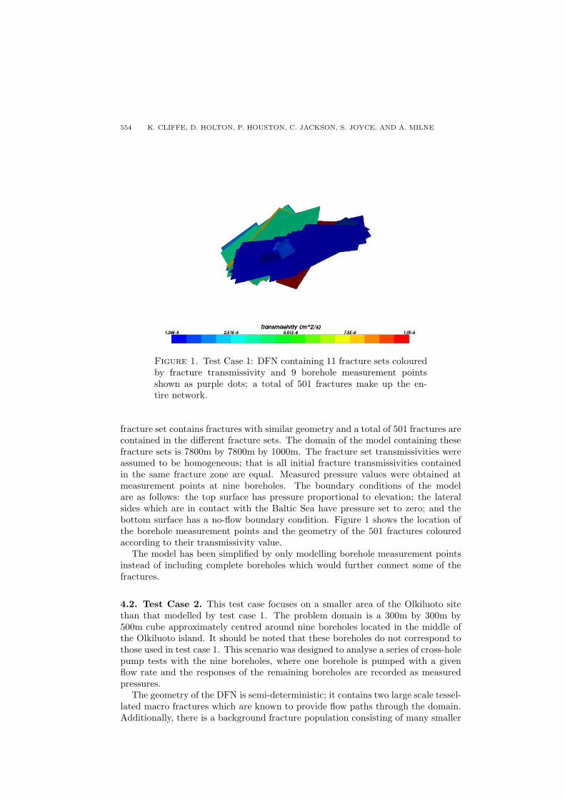
Figure 1. Test Case 1: DFN containing 11 fracture sets colouredby fracture transmissivity and 9 borehole measurement pointsshown as purple dots; a total of 501 fractures make up the en-tire network.

fracture set contains fractures with similar geometry and a total of 501 fractures arecontained in the different fracture sets. The domain of the model containing thesefracture sets is 7800m by 7800m by 1000m. The fracture set transmissivities wereassumed to be homogeneous; that is all initial fracture transmissivities containedin the same fracture zone are equal. Measured pressure values were obtained atmeasurement points at nine boreholes. The boundary conditions of the modelare as follows: the top surface has pressure proportional to elevation; the lateralsides which are in contact with the Baltic Sea have pressure set to zero; and thebottom surface has a no-flow boundary condition. Figure 1 shows the location ofthe borehole measurement points and the geometry of the 501 fractures colouredaccording to their transmissivity value.

The model has been simplified by only modelling borehole measurement pointsinstead of including complete boreholes which would further connect some of thefractures.

4.2. Test Case 2. This test case focuses on a smaller area of the Olkiluoto sitethan that modelled by test case 1. The problem domain is a 300m by 300m by500m cube approximately centred around nine boreholes located in the middle ofthe Olkiluoto island. It should be noted that these boreholes do not correspond tothose used in test case 1. This scenario was designed to analyse a series of cross-holepump tests with the nine boreholes, where one borehole is pumped with a givenflow rate and the responses of the remaining boreholes are recorded as measuredpressures.

The geometry of the DFN is semi-deterministic; it contains two large scale tessel-lated macro fractures which are known to provide flow paths through the domain.Additionally, there is a background fracture population consisting of many smaller


Figure 2. Test Case 2a: Domain of test case 2a with two tessel-lated macro fractures (macro fracture 1 and 2) intersected by nineboreholes. Macro fracture 1 is mainly green coloured with macrofracture 2 mainly blue coloured.

fractures throughout the domain. To study the effect of the background popula-tion, test case 2 has been split into two separate test cases. The same value ofmeasured pressures and measurement locations were used to condition the fracturetransmissivities in both of these test cases.

4.2.1. Test Case 2a. Test case 2a contains the two macro fractures, each tessel-lated into 900 sub-fractures. Here, zero pressure boundary conditions are used on allthe boundaries of the domain. The two macro fractures are shown in Figure 2 withthe hydraulic aperture (which is proportional to the cube of the fracture transmis-sivity) shown, as this shows the fracture tessellation more clearly. Macro fracture 1and macro fracture 2 have mean transmissivities estimated from field experimentsof 2.2E-4m2/s and 1.0E-5m2/s, respectively. The initial fracture apertures weregenerated by sampling from a normal distribution using corresponding aperturemeans to the transmissivity means. The initial transmissivities of the sub-fractureson each macro fracture were then assigned by converting the fracture apertures tofracture transmissivities using the cubic law [21].

The sub-fractures were assumed to be exponentially correlated. Defining theseparation Sij of two sub-fractures i and j as the distance between the centreof sub-fracture i and the centre of sub-fracture j, the standard deviation of sub-fracture log transmissivities as σX (assumed to be constant for all sub-fractureson the same macro fracture) and the correlation scale as ap, then the covariancematrix Ck of the sub-fractures transmissivities on macro fracture k is defined as

(34) Ck(i, j) =

σ2X , i = j ,

σ2X exp

−Sij

ap

, i 6= j .


Figure 3. Test Case 2b: Domain of test case 2b with two tessel-lated macro fractures intersected by nine boreholes and the addi-tion of a background fracture population.

4.2.2. Test Case 2b. In addition to the two tessellated macro fractures, a back-ground fracture population was added into the model domain providing additionalflow paths between the two macro fractures and the boreholes contained in themodel. A total of 24926 background fractures were included, whose statisticalproperties were derived from borehole orientation and location data. The main un-known of the background fracture population was the fracture size which was chosenso that the background fractures were large enough to make a well connected sys-tem between the macro fractures and the domain boundaries. The model domainis shown in Figure 3.

5. Results

In this section, we now present computational results to highlight the perfor-mance of the conditioning methods outlined in Section 3. Here, in addition tocomputing the (absolute) error ‖PM −Ph,M‖2 between the measured pressure val-ues, and those computed using each of the above conditioning algorithms, we shallalso compute the following relative error:

‖PM −Ph,M‖R =1

m

m∑

i=1

|(PM )i − Ph(Mi)|

(PM )i.

5.1. Test Case 1 Results. In this section, we assume that the fracture transmis-sivities are uncorrelated and accordingly set the covariance matrix C equal to the(n× n) identity matrix In.

5.1.1. Basis Vector Conditioning Results. In this section, we first considerthe application of the basis vector conditioning method to Test Case 1. To this end,Figure 4 compares the conditioned pressure to both the measured pressure and theinitial unconditioned pressures at all nine measurement points in test case 1. Itcan be seen that the conditioned pressures give a closer match to the measured


1 2 3 4 5 6 7 8 90

1

2

3

4

5

6

7

x 104

Measurement Point

Pre

ssur

e

Measured P

Unconditioned P

Conditioned P

Figure 4. Test Case 1. The measured pressures, unconditionedpressures and conditioned pressures at the nine measurementpoints using the basis vector conditioning algorithm.

‖PM −Ph,M‖2 ‖PM −Ph,M‖RInitial 1.1128E+5 0.6828Final 6.2327E+4 0.3574

Table 1. Test Case 1: Initial and final absolute and relative errorsusing the basis vector conditioning algorithm.

pressures at every measurement point compared to the unconditioned pressures,though an exact match is not achieved. In Table 1 we compute the initial andfinal absolute and relative errors between the calculated pressures and the mea-sured pressure values. Here, we clearly observe that the basis vector conditioningalgorithm yields a significant improvement in the computed pressure values whencompared to the initial (unconditioned) solution. Indeed, norms of the error areapproximately half of their initial values. It is clear that, while the conditionedpressures give a far better match to the measured pressures than the unconditionedpressures, the match is perhaps not as close as one would like; indeed, the finalrelative error is still around 36%, which is quite high. With this in mind, we nowproceed to apply the Bayesian algorithm to this test case.

5.1.2. Bayesian Conditioning Results. For all of the Bayesian conditioningresults presented in this article, we assume that each pressure measurement isindependent and that all measurements have the same standard deviation σP inthe measured pressure. Thus, the covariance matrix Σ from (31) takes the form

Σ = σ2P Im ,

where Im is the m×m identity matrix and the variance σ2P at a pressure measure-

ment point Mi, i = 1, . . . ,m, is defined as

σ2P = C((PM )i, (PM )i) = E(((PM )i − (PM )i)((PM )i − (PM )i)) ,


100

102

104

106

108

1010

0.1

0.2

0.3

0.4

0.5

0.6

0.7

0.8

Variance

Rel

ativ

e E

rror

Figure 5. Test Case 1: Variance σ2P of the pressure measurements

against the relative error using the Bayesian conditioning algo-rithm.

where C(·, ·) denotes the covariance, E(·) denotes the expectation and PM denotesthe mean value of the measured pressure. In Figure 5, we plot the relative erroragainst the variance of the pressure measurements σ2

P . It can be seen that therelative error possesses a minimum when the variance in the pressure measurementsis σ2

P = 1.0E+3; indeed, here ‖PM − Ph,M‖R = 0.1866. We recall, that this isaround half the relative error achieved when the basis vector conditioning method isemployed, cf. Section 5.1.1. However, as the variance in the pressure measurementsσ2P increases beyond a value of 1.0E+8, we observe that the relative error starts to

increase. This represents the point at which the standard deviation of the pressuremeasurements is of the same magnitude as the pressure measurements themselves(σP = 1.0E+4).

In order to improve the match to measured pressures even further, we considerthe following algorithm outlined below, which is based on adaptively selecting thevariance in the pressure measurements.

Algorithm 5.1. Updating the Variance.

(1) Set the initial fracture log transmissivities values X = X0 and set i = 0.(2) Run the Bayesian conditioning algorithm for step i on the fracture log trans-

missivities X with variance σ2P of the pressure measurements ranging from

1.0E+0 to 1.0E+10.(3) Take the conditioned log transmissivity values XC that correspond to the

variance value σ2P with the smallest final absolute error as the new initial

fracture transmissivities. That is set X = XC

(4) If the absolute error is below a given tolerance then stop. Otherwise, seti = i+ 1 and go to (2).

In Figure 6 we plot the variance σ2P in the measured pressure values against the

relative error for each step in Algorithm 5.1. Each point represents one run of theBayesian conditioning algorithm. Here, we observe that as the algorithm proceeds,the relative error in the computed pressures becomes relatively insensitive to the


Figure 6. Test Case 1: Variance σ2P of the pressure measurements

against the relative error for each iteration (step) of Algorithm 5.1.

Step ‖PM −Ph,M‖2 ‖PM −Ph,M‖RUnconditioned 1.1128E+5 0.6828

1 4.1522E+4 0.18662 1.4791E+4 0.05873 5.6679E+3 0.02434 4.7318E+3 0.01755 4.5264E+3 0.01586 4.3127E+3 0.01417 4.2446E+3 0.0133

Table 2. Test Case 1: Minimum absolute and relative errors ateach step of Algorithm 5.1.

specified value of the variance σ2P in the measured pressure values. Indeed, from

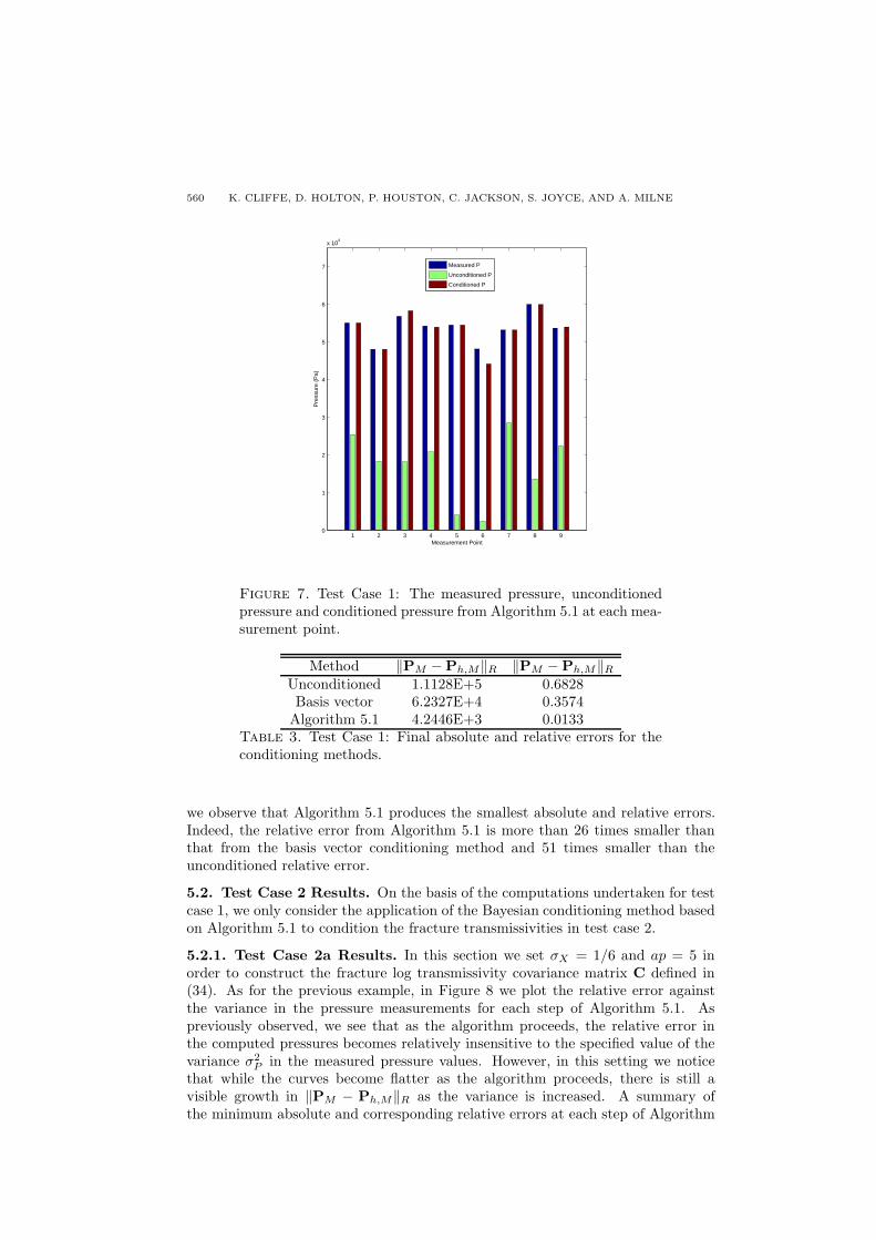
steps 4 onwards, the curves are essentially horizontal. Table 2 presents a summaryof the minimum absolute and relative errors at each step of Algorithm 5.1. Here, weobserve that both the absolute and relative errors converge to a relatively constantvalue after the first 4 steps of Algorithm 5.1 have been computed. In Figure 7we compare the conditioned pressures computed from step 7 of Algorithm 5.1 tothe unconditioned and measured pressures. Here, we clearly observe the excellentmatch that has been attained based on employing Algorithm 5.1. Indeed, withthe exception of the third and sixth measurement points, the measured pressure isalmost identically matched at the other seven measurement points.

Finally, in Table 3 we compare the final absolute and relative errors of the twonewly proposed conditioning methods applied to test case 1. As already noted,


1 2 3 4 5 6 7 8 90

1

2

3

4

5

6

7

x 104

Measurement Point

Pre

ssur

e (P

a)

Measured P

Unconditioned P

Conditioned P

Figure 7. Test Case 1: The measured pressure, unconditionedpressure and conditioned pressure from Algorithm 5.1 at each mea-surement point.

Method ‖PM −Ph,M‖R ‖PM −Ph,M‖RUnconditioned 1.1128E+5 0.6828Basis vector 6.2327E+4 0.3574Algorithm 5.1 4.2446E+3 0.0133

Table 3. Test Case 1: Final absolute and relative errors for theconditioning methods.

we observe that Algorithm 5.1 produces the smallest absolute and relative errors.Indeed, the relative error from Algorithm 5.1 is more than 26 times smaller thanthat from the basis vector conditioning method and 51 times smaller than theunconditioned relative error.

5.2. Test Case 2 Results. On the basis of the computations undertaken for testcase 1, we only consider the application of the Bayesian conditioning method basedon Algorithm 5.1 to condition the fracture transmissivities in test case 2.

5.2.1. Test Case 2a Results. In this section we set σX = 1/6 and ap = 5 inorder to construct the fracture log transmissivity covariance matrix C defined in(34). As for the previous example, in Figure 8 we plot the relative error againstthe variance in the pressure measurements for each step of Algorithm 5.1. Aspreviously observed, we see that as the algorithm proceeds, the relative error inthe computed pressures becomes relatively insensitive to the specified value of thevariance σ2

P in the measured pressure values. However, in this setting we noticethat while the curves become flatter as the algorithm proceeds, there is still avisible growth in ‖PM − Ph,M‖R as the variance is increased. A summary ofthe minimum absolute and corresponding relative errors at each step of Algorithm


Figure 8. Test Case 2a: Plot of the relative error against variancein the pressure measurements for each step of Algorithm 5.1.

Figure 9. Test Case 2a: Conditioned pressures after step 5 of Al-gorithm 5.1 at each measurement point compared to the measuredand unconditioned pressure values.

5.1 are shown in Table 4 for this test case. Here, we now observe that after 5steps of Algorithm 5.1, the conditioned pressures provide an excellent match tothe measured pressures. Indeed, this is clearly visible in Figure 9, where we plotthe final conditioned pressures after step 5 of Algorithm 5.1, together with theunconditioned and measured values at each measurement point.



1 3.8363E+4 0.40942 1.3904E+4 0.16953 7.9760E+3 0.12424 1.9890E+3 0.04295 8.1150E+1 0.0007

Table 4. Test Case 2a: Minimum absolute and relative errors ateach step of Algorithm 5.1.


1 4.0773E+4 1.08122 1.5625E+4 0.73183 4.1325E+3 0.09604 1.6182E+2 0.0048

Table 5. Test Case 2b: Minimum absolute and relative errors ateach step of Algorithm 5.1.

5.2.2. Test Case 2b Results. This final test case involves a total of 26727 frac-ture transmissivities which need to be conditioned. Given the size of this problem,it was computationally too expensive to run the Bayesian conditioning algorithm tocondition every fracture transmissivity. Instead, fractures to be conditioned wereselected depending on their sensitivity values. To this end, fractures that had a sen-sitivity value of 1.0 or greater with respect to any of the measured pressures wereselected for conditioning. This resulted in 2205 fracture transmissivities (with thegreatest sensitivity values) being conditioned, while leaving the remaining fracturetransmissivities constant at their initial value throughout the Bayesian conditioningalgorithm. In other words, only selected fracture transmissivities were conditionedbut pressure values were re-calculated using all of the fracture transmissivities inthe DFN (including those held constant). Furthermore, due to the computationaltime taken to perform the conditioning of fracture transmissivities, the values ofσ2P in each step of Algorithm 5.1 were limited to 1.0E+3, 1.0E+4, 1.0E+5, and

1.0E+6. This selection was based on results from the previous test cases where novalues of σ2

P less than 1.0E+3 or greater than 1.0E+6 minimised the absolute errorat any step of Algorithm 5.1.

In Table 5 we show the minimum absolute and relative errors for each step ofAlgorithm 5.1 for test case 2b. The relative error at steps 1 and 2 are higher thanwould be expected compared to the previous test cases. This was due to the smallmeasured pressure value at measurement point 8. At steps 1 and 2 the conditionedpressure at measurement point 8 was considerably higher than the measured pres-sure which greatly affected the value of ‖PM−Ph,M‖R. Notwithstanding this issue,we see that after 4 steps of Algorithm 5.1, the relative error is less than 0.5%. In-deed, Figure 10 clearly highlights the excellent match with the measured pressuresattained by the conditioned pressures. For completeness, in Figure 11 we plot theabsolute error against the variance in the pressure measurements for each step ofAlgorithm 5.1; the absolute error was chosen, rather than the relative error, due tothe issue with measurement point 8 outlined above.


1 2 3 4 5 6 7 8 90

1

2

3

4

5

6

7x 10

4

Measurement Point

Pre

ssur

e (P

a)

Measured P

Unconditioned P

Conditioned P

Figure 10. Test Case 2b: Conditioned pressures after step 4 ofAlgorithm 5.1 at each measurement point compared to the mea-sured and unconditioned pressure values.

103

104

105

106

0

1

2

3

4

5

6

7

8x 10

4

Variance

Abs

olut

e E

rror

step1

step2

step3

step4

Figure 11. Test Case 2b: Plot of the absolute error against vari-ance in the pressure measurements for each step of Algorithm 5.1.

6. Summary and Conclusion

In this article, we have presented two new conditioning methods which are capa-ble of conditioning fracture transmissivities in a DFN on measured pressure values.


The first approach is based on the computation of suitable basis vectors, togetherwith the solution of a nonlinear optimisation problem. This method represents theextension of the work, undertaken by Cliffe and Jackson [3, 4] in the context ofcontinuous porous media problems, to DFNs. The second approach outlined is aBayesian conditioning method that calculates a mode (point of highest likelihoodfor the fracture transmissivities given the measured pressures) of the posterior dis-tribution of the fracture transmissivities numerically. Both methods have beennumerically tested on a potential site for nuclear waste disposal at the Olkiluotosite in Finland. While both conditioning methods improved the match of the com-puted pressures to the measured experimental values, the Bayesian approach wasseen to be superior, in the sense that it gave rise to the smallest relative errorbetween the measured and conditioned pressures, evaluated at the measurementpoints. This method was further tested on a smaller area of the Olkiluoto site. Inthis setting, we considered two cases: firstly, when the DFN consists of only twolarge tessellated fractures, and secondly, when these two large tessellated fracturesare supplemented by a background fracture population. In both cases, the Bayesianconditioning method provided an excellent match to the measured pressure values.

References

[1] J. Bear. Dynamics of Fluids in Porous Media. Elsevier, New York, 1972.[2] J. Carrera and S. P. Neuman. Estimation of aquifer parameters under transient and steady

state conditions: 1. Maximum liklihood method incorporating prior information. Water Re-

sour. Res., 22(2):199–210, 1986.[3] K.A. Cliffe and C.P. Jackson. Conditioning stochastic groundwater flow models on head data.

In Materials Research Society Symposium Proceedings, volume 353, page 7, 1995.[4] K.A. Cliffe and C.P. Jackson. A new method for conditioning stochastic groundwater flow

models on head data. Technical report, Harwell, AEA Technology, 2000.[5] A. Frampton and V. Cvetkovic. Inference of field-scale fracture transmissivities in crystalline

rock using flow log measurements. Water Resour. Res., 46:W11502, 2010.[6] A. Frampton, V. Cvetkovic, and D. Holton. Aspo task force on modeling of groundwater flow

and transport of solutes - Task 7A, Task 7A1 and 7A2: Reduction of performance assessmentuncertainty through modeling of hydraulic tests at Olkiluoto, Finland. Technical report, 2008.

[7] L. Koskinen H. Ahokas. Task 7: Modelling the KR24 long-term pumping test at Olkiluoto.Technical report, 2005.

[8] L. Hartley. NAPSAC release 9.3 technical summary document. Technical report, Serco As-surance, 2000.

[9] M.C. Hill and C.R. Tiedeman. Effective Groundwater Model Calibration. John Wiley & Sons,2007.

[10] L. Jing. A review of techniques, advances and outstanding issues in numerical modelling forrock mechanics and rock engineering. Int. J. Rock Mech. Min., 40:283–353, 2003.

[11] P.K. Kitanidis. On the geostatistical approach to the inverse problem. Adv. Water Resour.,19(6), 1996.

[12] R. Marrett. Aggregate properties of fracture populations. J. Struct. Geol., 18(2/3):9, 1996.[13] A. Milne. Topics in Flow in Fractional Media. PhD thesis, School of Mathematical Sciences,

University of Nottingham, 2011.[14] S.P. Neuman. Calibration of distributed parameter groundwater flow models viewed as a

multiple-objective decision process under uncertainty. Water Resour. Res., 9(4):1006–1021,1973.

[15] S.P. Neuman, G.E. Hogg, and E.A. Jacobson. A statistical approach to the inverse problem

of aquifer hydrology: 2. Case study. Water Resour. Res., 16(1):33–58, 1980.[16] W.H. Press, B.P. Flannery, S.A. Teukolsky, and W.T. Vetterling. Numerical Recipes. Cam-

bridge University Press, 1986.[17] D. T. Snow. The frequency and apertures of fractures in rock. Int. J. Rock Mech. Min.,

7:23–40, 1970.[18] A.M. Stuart. Inverse problems: A Bayesian perspective. In A. Iserles, editor, Acta Numerica,

pages 451–559. Cambridge University Press, 2010.


[19] C.R. Tiedeman, D.J. Goode, and P.A. Hsieh. Characterizing a groundwater basin in a newengland mountain and valley terrain. Ground Water, 36(4):611620, 1998.

[20] R.M. Yager. Simulated three-dimensional groundwater flow in the lockport group, a fractures-dolomite aquifer near Niagara Falls, New York. Technical report, USGS Water ResourcesInvestigation Report 924189, U.S. Geological Survey, Reston, Va., 1993.

[21] R.W. Zimmerman and G.S. Bodvarsson. Hydraulic conductivity of rock fractures. TransportPorous Med., 23(1):1–30, 1996.

School of Mathematical Sciences, University of Nottingham, University Park, Nottingham,NG7 2RD, UK.

E-mail : [email protected]

Serco, Harwell, UKE-mail : [email protected]







CONDITIONING DISCRETE FRACTURE NETWORK MODELS OF GROUNDWATER FLOW

Documents

Transcript of CONDITIONING DISCRETE FRACTURE NETWORK MODELS OF GROUNDWATER FLOW