Conditional-logit Bayes estimators for consumer valuation ofelectric vehicle driving range

Ricardo A. Daziano

School of Civil and Environmental Engineering, Cornell University, 305 Hollister Hall, Ithaca, NY14853.

Abstract

Range anxiety – consumers’ concerns about limited driving range – is generally con-sidered an important barrier to the adoption of electric vehicles. If consumers cannotovercome these fears it is unlikely that they will consider purchasing an electric car.Hence, for planning a successful introduction of low emission vehicles in the market itbecomes essential to fully understand consumer valuation of driving range. Analyzingexperimental data on vehicle purchase decisions in California, in this paper I derive andstudy the statistical behavior of Bayes estimates that summarize consumer concernstoward limited driving range. These estimates are superior to the marginal utilities asparameters of interest in a discrete demand model of vehicle choice. One of the empiricalresults is the posterior distribution of the willingness to pay for electric vehicles withimproved batteries offering better driving range. Credible intervals for this willingness topay, as well as both parametric and nonparametric heterogeneity distributions are alsoanalyzed.

Keywords: Bayesian discrete choice; battery electric vehicles; range anxiety;heterogeneity distributionsJEL classification: C25, D12, Q42, Q50

Email addresses: daziano@cornell.edu (Ricardo A. Daziano), Phone: (1) 607 255-2018 -Fax: (1) 607 255-9004 (Ricardo A. Daziano)

Preprint submitted to Resource and Energy Economics November 15, 2012

1. Introduction1

Improvements in energy efficiency of car engines represent a relevant step toward sus-2

tainability in personal transportation. However, ultra-low-emission vehicles still have3

numerous drawbacks when compared to their standard gasoline counterparts. For in-4

stance, high purchase price, limited driving range, lack of recharging stations and lengthy5

recharging may prevent consumers from adopting battery electric vehicles. Thus, private6

investments, subsidy programs, or both may be needed to support initial consumer ac-7

ceptance of electric vehicles in the automotive market. For planning these investments8

and subsidies, it becomes critical to economically valuate the impact of the current9

limitations of ultra-low-emission vehicles on consumer conversion to alternative energy10

technologies.11

To derive measures of consumer valuation of driving range of electric vehicles, in this12

paper I use stated-preference microdata on vehicle choice in California and I revisit13

estimation of the conditional1 logit model (McFadden, 1974), but from a Bayesian per-14

spective. The logit model has been labeled as the workhorse of discrete choice modeling,15

as it represents an ideal, fully-specified model and actually was the most used model16

since the earliest developments in the field from the 1970s until the mid 1990s. Prop-17

erties and limitations of the logit model are well understood, and more flexible models18

that account for more general covariance structures have been derived. However, there19

are at least two reasons to revisit estimation of the logit model. First, a logit model can20

form the kernel of a more complex model, such as a hybrid choice model with a logit21

kernel that accounts for unobserved heterogeneity. In fact, the logit model is the kernel22

of the mixed logit model (McFadden and Train, 2000), which is the current workhorse23

of discrete choice modeling. Second, within the extremely limited number of applica-24

tions of the Bayesian approach to discrete choice modeling of travel behavior, there is25

practically no discussion of Bayesian estimation of the traditional logit with fixed param-26

eters (without addressing random consumer heterogeneity). In addition, the estimation27

of heterogeneity distributions is being dominated by parametric assumptions, and almost28

exclusively using frequentist estimators (one exception being Train and Sonnier, 2005).29

This paper adds to the empirical literature on Bayesian inference in discrete choice mod-30

eling by analyzing different samplers for Markov chain Monte Carlo (MCMC) estimation31

of conditional logit models, assuming not only a homogenous sample via fixed parameters32

but also accounting for both parametric and nonparametric heterogeneity distributions.33

1Depending on the nature of the regressors, the econometric literature distinguishes the multinomiallogit model from the conditional logit model. The multinomial logit model considers individual-specificregressors, whereas the conditional logit model considers alternative-specific attributes. Nevertheless,this distinction is somewhat artificial. In fact, in travel behavior modeling a multinomial logit modelusually refers to what econometricians call conditional logit.

2

Based on a convergence analysis, it was determined that an independence Metropolis34

Hastings sampler was faster and had better performance in terms of lower autocorre-35

lation than a random walk or slice sampling. The analysis of this paper differs from36

previous research as I propose to study the posterior behavior of estimators of nonlinear37

transformations of the model parameters. This analysis is motivated by the possibility38

of deriving transformed parameters – such as willingness to pay – that are superior to39

the marginal utilities as parameters of interest in a discrete choice model, as these trans-40

formations have a direct economic interpretation. In addition, since willingness to pay41

is a parameter that is locally almost unidentified, it is not clear whether convergence of42

the marginal utilities will ensure convergence of their ratios. This first contribution is43

relatively general in scope in the sense that the methodology for obtaining and analyzing44

the results is applicable to any discrete choice problem. In fact, based on these results an45

independence Metropolis Hastings estimator was used as the sampler for the population46

parameters of the hierarchical model that allows for random consumer heterogeneity.47

The main contribution of this paper is empirical. Effectively, the Bayes estimators are48

applied to the problem of consumer valuation of electric vehicle attributes, with a spe-49

cial focus on driving range. I propose to derive from the estimates of the discrete choice50

demand model four specific driving-range-valuation measures, namely the willingness51

to pay for marginal driving range improvements (see Hidrue, Parsons, Kempton, and52

Gardner, 2011, Dimitropoulos, Rietveld, and van Ommeren, 2012), the compensating53

variation after improvements in range (cf. Dimitropoulos et al., 2012), the elasticity of54

the choice probability of buying an electric vehicle with respect to marginal range im-55

provements, and a measure of range equivalency (cf. Hess, Train, and Polak, 2006). These56

four proposed measures are economically meaningful functions of the marginal utilities57

and – even though these functions can also be derived in a frequentist context – statis-58

tical inference (point and interval estimation) on these nonlinear functions is facilitated59

by the use of Markov chain Monte Carlo methods. This work combines technical and60

empirical contributions by using post-processing (Sonnier, Ainslie, and Otter, 2007) of61

the posterior distributions of the marginal utilities to identify robust confidence inter-62

vals for inference on the driving-range-valuation measures. In the context of parameter63

transformations, frequentist econometric methods encounter problems due to parameters64

that may be weakly identified (Bolduc, Khalaf, and Yélou, 2010). Because the Bayesian65

approach is proving to be a compelling solution to this problem, I adopt these promising66

techniques to analyze willingness to pay and other economic measures derived from the67

estimates of a discrete demand model. Whereas working with a model in willingness-68

to-pay space produces direct confidence intervals of willingness to pay, recasting the69

parameter space does not solve the problem of estimating intervals of other functions of70

the parameters, such as elasticities, choice probabilities, or welfare measures.71

The empirical analysis of this work shows that the willingness to pay for driving range72

decreases with range and for current market conditions – i.e. electric vehicles that can73

be driven for 100 miles on a single charge – is around 100 $/mile (cf. to the median of74

3

58 $/mile found in Dimitropoulos et al. (2012)), whereas the marginal cost of producing75

a lithium-ion battery with improved range is about 110 $/mile.276

The rest of the paper is organized as follows. Section 2 first overviews the data and then77

introduces measures for valuation of consumer concerns toward limited driving range.78

The data comes from stated vehicle-type choices, including low-emission alternatives, by79

consumers in California. Consumer valuation of driving range is then defined via nonlin-80

ear functions of the marginal utilities representing how consumers react to driving range81

improvements in terms of willingness to pay, compensating variation, and elasticity of82

the choice probability of buying an electric car. Section 4 presents the empirical analysis83

of the Bayes estimates of the marginal utilities and of the range valuation measures.84

These measures are then extended to better represent the tradeoffs among higher pur-85

chase prices, limited range, and transportation costs savings. Section 5 concludes and86

offers some insights for future work. In Appendix A, details regarding the derivation of87

the Bayes estimators are discussed.88

2. Consumer adoption of electric vehicles89

2.1. Electric vehicles and driving range anxiety90

Electric vehicles are propelled by one or more electric motors that are powered by91

rechargeable electric vehicle batteries. Since standard vehicles that are powered by in-92

ternal combustion rely on fossil fuels – with the concomitant negative externalities –93

electric vehicles have been identified as an alternative to promote sustainable personal94

transportation. Because electric vehicles have the potential for being charged using clean95

energy sources, a conversion to electric vehicles is usually regarded as a path toward an96

independent, cleaner, and more secure energy future. Even if the electricity comes from97

sources that are not environmentally friendly, such as coal, vehicles with zero tailpipe98

emissions still have associated benefits such as reducing direct pollution sources in an99

urban context. This includes reduced air pollutants and reduced traffic noise in cities.100

Electric motors are in general more efficient than those propelled by internal combustion.101

Additionally, the conversion to clean energy could be boosted by an increasing penetra-102

tion of electric vehicles. However, current technologies for electric vehicles have a series103

of limitations that may prevent broad consumer adoption.104

In particular, current electric vehicles suffer from a limited driving range, which can105

be defined as the maximum distance allowed by a full battery charge. Consumer con-106

cerns toward the limited driving range of electric vehicles are increased because of long107

2Dollars of 2005 for direct comparisons.

4

recharging times3 and lack of recharging stations.4 These concerns are summarized into108

what has been called range anxiety or the consumer fear that the electric vehicle battery109

will exhaust while driving. These fears represent a major problem for the introduction110

of electric vehicle into the market: if consumers continue to suffer driving range anxiety111

it is unlikely that they will consider the purchase of an electric car.112

Both high purchase prices and high maintenance costs, including battery replacements,113

also appear as barriers for the adoption of electric vehicles. Table 1 displays three electric114

vehicles that are currently being offered in the US market.

Estimated Energy In the US Units soldMake & Model MSRP* [US$] driving range efficiency** since in the US***Nissan LEAF 32,780 100 miles 99 [mpge] 2011 14,905Chevrolet Volt**** 40,280 35 miles 94 [mpge] 2011 24,345Tesla Roadster 109,000 245 miles 120 [mpge] 2010 2,350Toyota Prius 24,000 536 miles 50 [mpg] 2000 1,200,500* Starting manufacturer’s suggested retail price does not include federal tax savings.** EPA combined fuel economy.*** Until September 2012. In the case of the Tesla Roadster, the figure represents worldwide sales of the total fixed numberthat was produced.**** The Chevy Volt is technically an extended range electric vehicle that works on gas when the electric battery is exhausted.The figures represent all-electric operation.Source: specifications provided by the respective manufacturer.

Table 1: Electric vehicles widely available in the US market in 2012. (Figures for a hybrid powertrainare added for reference.)

115

Note that all three vehicles have suggested retail prices that exceed the average price116

of new cars, which was 28,400 US$ in 2010 (National Automobile Dealers Association,117

2010). Although the actual expenditure is lower, because of a 7,500 US$ electric vehicle118

federal tax credit as well as additional state discounts, the cost of electric cars is still119

high for the offered body type.120

The actual first figures of deliveries for the Nissan LEAF and the Chevrolet Volt may121

disappoint enthusiasts who are expecting an electric car revolution: from introduction122

into the market in December 2010 until February 2011 Nissan sold 173 LEAFs (Nissan,123

2011) and Chevrolet, 928 Volts (General Motors, 2011).5 However, because both models124

are in an extremely early stage of market penetration,6 it is too early to assess whether125

consumers are not interested in adopting electric vehicles or how driving range anxiety126

may be influencing consumer choices.127

3Recharging the electric vehicle battery with standard outlets can take from 8 to 16 hours.4Standard vehicles also have a limited driving range. However, the high availability of gas service

stations as well as extremely short refueling times allow consumers to ignore driving range limits offossil fuel-powered vehicles.

5In 2011, NISSAN sold a total of 9674 LEAFs and Chevrolet sold 7671 Volts.6The Tesla Roadster is a luxurious sports car with intended limited production.

5

2.2. Discrete choice models of electric vehicle purchase decisions128

Microeconometric models of private vehicle purchase decisions involving alternative en-129

ergy sources in the choice set have a long tradition (see Daziano and Chiew, 2012, for130

a review of these models). Just a couple of years after the first applications of discrete131

choice models to standard vehicle choice, the seminal work of Beggs and Cardell (1980)132

and Beggs, Cardell, and Hausman (1981) set the basis for later empirical research. When133

analyzing demand for electric vehicles using random utility maximization, non-standard134

attributes such as driving range (Bunch, Bradley, Golob, Kitamura, and Occhiuzzo, 1993,135

Brownstone, Bunch, and Train, 2000, Ewing and Sarigöllü, 1998, Hidrue et al., 2011),136

availability of charging stations (Bunch et al., 1993, Brownstone et al., 2000, Achtnicht,137

2012), and time for recharging (Golob, Torous, Bradley, Brownstone, Crane, and Bunch,138

1997, Ewing and Sarigöllü, 1998) become relevant. This new set of attributes allows re-139

searchers to study consumer valuation of, for instance, improved electric batteries offering140

extended driving range.141

Willingness to pay for marginal improvements in driving range is an economic mea-142

sure of the tradeoff between purchase price and driving range of electric vehicles (see143

Dimitropoulos et al., 2012), which is a key input for welfare and cost-benefit analysis144

of investments in improving electric batteries. Inference on willingness to pay can be145

derived from the estimates of discrete choice models. Table 2 provides a summary of146

different willingness-to-pay estimates for a one-mile improvement in driving that have147

been derived for the American market (estimates for other markets are also summarized148

in Dimitropoulos et al., 2012).149

WTP [US$05/mile]Main References Market Mean est. Min est. Max est.Beggs and Cardell (1980), Beggs et al. (1981) US (1978) 85 61 132Calfee (1985) California (1980) 195 195 195Bunch et al. (1993) California (1991) 101 95 106Brownstone et al. (2000) California (1993) 99 58 202Golob et al. (1997) California (1994) 117 76 202Tompkins, Bunch, Santini, Bradley, Vyas, and Poyer (1998) US (1995) 64 44 102Train and Hudson (2000), Train and Sonnier (2005) California (2000) 100 87 131Hess, Fowler, Adler, and Bahreinian (2012) California (2008) 43 36 49Hidrue et al. (2011) US (2009) 64 47 82Nixon and Saphores (2011) US (2010) 182 46 317

Table 2: Willingness to pay estimates for marginal improvements in driving range. Results from differentstudies in the US (Source: Dimitropoulos et al., 2012)

6

3. A conditional logit model of vehicle choice in California150

3.1. Data151

To understand the tradeoffs that control the adoption of low-emission vehicles, including152

concerns toward limited driving ranges of electric cars, I use stated-preference data on153

vehicle choice in California as reported by Train and Hudson (2000).7154

Participants of the survey were sampled from residents of California who were prospective155

buyers of a new vehicle. Each of the 500 respondents in the survey answered up to 15156

experimental choice situations between three vehicle alternatives.8 The sample contains a157

total of 7437 observations. Respondents in the sample were provided with information on158

electric vehicles and on air quality in California. Additionally, respondents were provided159

with detailed information regarding performance of the vehicles, including top speed and160

total of seconds required to reach a speed of 60 mph. For each vehicle, the experimental161

attributes were defined as:162

• Energy source [gas internal combustion, electric, gas-electric hybrid]163

• Purchase price [thousands of US dollars]164

• Operating cost [US dollars per month]165

• Driving range for electric vehicles [hundreds of miles]166

• Performance [high, medium, low]167

• Body type [mini car, small car, mid car, large car, small SUV, mid SUV, large168

SUV, compact PU, full PU, minivan]169

The actual attribute values in the stated preference experiment were set following a170

randomized design: after defining the possible attribute levels, each choice situation was171

specified by randomly selecting from the levels of each attribute. Because the experiment172

was unlabeled and energy source (engine type) was chosen randomly for each vehicle in173

each choice situation, the respondent faced a random combination of engine types at174

every choice experiment (e.g. two gasoline and one hybrid vehicle, or among one gasoline175

and two electric vehicles, or any other combination). Purchase prices and operating176

costs were chosen randomly from a range of plausible prices and fuel costs for each177

combination of body type and energy source. For high performance, a top speed of 120178

mph and 8 seconds to reach 60 mph was considered. Medium performance was set at top179

speed of 100 mph and 12 seconds to reach 60 mph. Low performance was defined as top180

speed of 80 mph and 16 seconds to reach 60 mph. For electric vehicles, performance was181

7Details regarding the design of the survey, and data collection and analysis, can be found in Trainand Hudson (2000). This dataset has also been used by Sándor and Train (2004), Train and Sonnier(2005), and Hess et al. (2006)

8The experimental design considered unlabeled alternatives.

7

randomly selected from the medium and low levels. A constant level of driving range182

was considered for both internal combustion engine and hybrid vehicles. In the case183

of electric cars, driving range was chosen randomly from a set of 10 mile increments184

within the bounds of 60 and 200 miles. Finally, whereas in the first 7 experiments for185

each respondent body type was chosen randomly for each vehicle from the ten possible186

builds, in the last 8 experiments one body type was chosen randomly and kept the same187

for all three vehicles in the choice situation. A summary of the randomized design of the188

choice experiment is displayed in table 2, and Appendix B presents a sample of a choice189

situation as seen by respondents of the survey.190

Gas Hybrid ElectricPurch. price Op. cost Purch. price Op. cost Purch. price Op. cost Driving range[1,000$] [$/month] [1,000$] [$/month] [1,000$] [$/month] [100 miles]

Mean 22.40 48.86 42.88 30.10 42.93 20.61 1.30Stdv 7.37 11.99 17.50 10.20 17.66 9.58 0.40Min 7.02 17.58 10.02 7.52 10.02 2.51 0.60Max 38.93 72.11 97.30 52.31 97.26 42.30 2.00

Table 3: Data descriptive statistics resulting from the randomized experimental design

The experimental levels reflect relatively realistic choice situations when compared to191

current vehicles offered in the market. Note that the average experimental electric driving192

range is 130 miles, with bounds that reflect current supply, and the average price of193

$42,930 for the purchase of an electric vehicle in the experiment is of the same magnitude194

of the current price of the Volt. This shows that even though the data is somewhat dated,195

the experimental situation still accurately reflects current real-world situations.196

3.2. Valuation of consumer concerns toward limited driving range197

In this paper, a conditional logit model of vehicle purchase decisions is proposed to un-198

derstand the factors that explain demand for low-emission vehicles. Thus, I consider a199

random indirect utility is defined as Uint = x′intθ + εint, where i ∈ {1, 2, 3}, n represents200

the individual, and t the choice situation. The iid structure of the kernel covariance201

matrix is justified by the fact that the experiment was designed with unlabeled alter-202

natives. However, to account for the repeated observation problem that is intrinsic to203

stated-preference experiments, I use individual-specific realizations of the random taste204

parameters for the choice situations answered by the same individual.205

Regarding the attribute levels contained in xint, note that among the attributes only206

purchase price, operating cost, and driving range are continuous variables. The rest are207

defined as index functions. For energy source, gas internal combustion is set as base. The208

same applies for medium performance and mid-car body type. Since the experiment was209

unlabeled, the model does not contain alternative specific constants ASCi.210

8

Most previous studies – including Sándor and Train (2004), Train and Sonnier (2005),211

and Hess et al. (2006) who use the same vehicle choice data of this work – have specified212

marginal utilities of driving range that are constant. The underlying assumption is that213

both willingness to pay for and consumer surplus from improvements in driving range214

are constant. It is easy to argue that driving range should exhibit diminishing returns,215

meaning that an additional mile in driving range for a vehicle that currently offers 80216

miles should provide more utility than an additional mile for a 200-mile range vehicle.217

Following the work of Calfee (1985), a logarithmic transformation of driving range was218

applied (see also Kavalec, 1999, Hess et al., 2012).219

Using the definition of attributes discussed in the paragraphs above, the dimension of220

both xint and θ is 16.221

The proposed demand model of vehicle choice can be used to derive insights into con-222

sumer valuation of driving range. Let θpp be the marginal utility of purchase price, θoc223

the marginal utility of operating costs, θln range the marginal utility of the logarithmic224

transformation of driving range of electric vehicles, and θBEV the constant specific to225

battery electric vehicles. It is then possible to define the following functions:226

1. Willingness to pay for driving range improvements (WTP∆range): marginal rate of227

substitution of driving range and purchase price9228

WTP∆range = −∂UBEV /∂range∂U/∂pp

= −θln range

θpp

1

range. (1)

Note that because of the logarithmic transformation of range, WTP∆range is not229

just a parameter ratio but also a nonlinear function of the range level.230

2. Compensating variation after driving range improvements (CV∆range): welfare-231

analysis measure that represents the change in income needed to offset changes232

in utility after a change in driving range of ∆range,233

CV∆range = − 1

θpp

[ln

J∑i=1

exp(x

(1)′

int θ)− ln

J∑i=1

exp(x

(0)′

int θ)]

, (2)

where x(1)int−x

(0)int = ln(range+∆range)−ln(range). (Equation (2) is the well-known234

expression of the expected compensating variation for logit models.) This measure235

is a relevant input for informing policymakers, as it can be used for evaluating236

welfare improving effects of subsidies for automakers to improve battery capacities,237

reduce cost of battery production, or both.238

3. Elasticity of the choice probability of buying an electric vehicle with respect to239

9WTP∆range represents how much more a consumer is willing to pay for buying an electric car thatoffers an additional 100 miles before recharging.

9

marginal driving range improvements (EPEV ,range): individual-specific measure of240

the percentage increase in the choice probability of choosing an EV (PEV,n) after241

a marginal improvement of a one-percent change in driving range242

EPBEV ,range = θln range(1− PBEV,n). (3)

i.e. the purchase price reductions that ensure that a consumer is willing to accept243

the limited driving range while keeping the same utility level as an internal com-244

bustion vehicle. Elasticities inform automakers about what to expect in terms of245

marginal improvements in market shares after improved batteries are introduced.246

Note that because of the logarithmic transformation of range, the resulting elas-247

ticity depends only on the parameter of the attribute of interest (in this case the248

logarithm of range) and the electric-vehicle choice probability.249

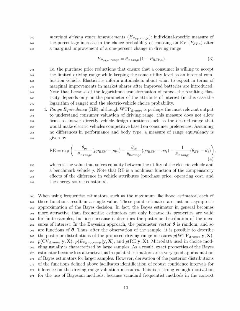
4. Range Equivalency (RE): although WTP∆range is perhaps the most relevant output250

to understand consumer valuation of driving range, this measure does not allow251

firms to answer directly vehicle-design questions such as the desired range that252

would make electric vehicles competitive based on consumer preferences. Assuming253

no differences in performance and body type, a measure of range equivalency is254

given by255

RE = exp

(− θppθln range

(ppBEV − ppj)−θoc

θln range

(ocBEV − ocj)−1

θln range

(θEV − θj)),

(4)which is the value that solves equality between the utility of the electric vehicle and256

a benchmark vehicle j. Note that RE is a nonlinear function of the compensatory257

effects of the difference in vehicle attributes (purchase price, operating cost, and258

the energy source constants).259

When using frequentist estimators, such as the maximum likelihood estimator, each of260

these functions result in a single value. These point estimates are just an asymptotic261

approximation of the Bayes decision. In fact, the Bayes estimator in general becomes262

more attractive than frequentist estimators not only because its properties are valid263

for finite samples, but also because it describes the posterior distribution of the mea-264

sures of interest. In the Bayesian approach, the parameter vector θ is random, and so265

are functions of θ. Thus, after the observation of the sample, it is possible to describe266

the posterior distributions of the proposed driving range measures p(WTP∆range|y,X),267

p(CV∆range|y,X), p(EPBEV ,range|y,X), and p(RE|y,X). Microdata used in choice mod-268

eling usually is characterized by large samples. As a result, exact properties of the Bayes269

estimator become less attractive, as frequentist estimators are a very good approximation270

of Bayes estimators for larger samples. However, derivation of the posterior distributions271

of the functions defined above facilitates identification of robust confidence intervals for272

inference on the driving-range-valuation measures. This is a strong enough motivation273

for the use of Bayesian methods, because standard frequentist methods in the context274

10

of nonlinear functions of the model parameters face the problem of weak identification275

(Bolduc et al., 2010).276

4. Empirical analysis of the Bayes estimators277

4.1. Bayes estimates of vehicle purchase preferences278

Three logit-based econometric models of vehicle choice behavior were considered, namely279

a conditional logit model with fixed parameters (no random consumer heterogeneity) and280

two models that account for a heterogeneity distribution of parameters. For the latter281

two both a parametric and a nonparametric assumption was made for the heterogene-282

ity distribution, leading to a parametric random parameter logit and a semiparametric283

random parameter logit, respectively. Table 4 presents the population point estimates of284

the choice model parameters for the three Bayes estimators considered. The results are285

based on 50,000 iterations after a burn-in of 5,000 initial draws. Total length of the runs286

were determined using Raftery-Lewis estimates (Raftery and Lewis, 1992).287

Fixed param. Parametric Nonparametriclogit heterogeneity heterogeneity

Attribute θ̂ s.d. θ̂ s.d. θ̂ s.d.Purchase price -0.0533 0.002 -0.1879 0.008 -0.1228 0.004Operating cost -0.0266 0.002 -0.0693 0.004 -0.0478 0.003ln Driving range 0.6082 0.095 1.7154 0.241 1.1706 0.138Electric -0.2648 0.114 -0.1890 0.256 -0.2088 0.178Hybrid 0.4128 0.057 1.5134 0.127 1.0482 0.095High performance 0.1220 0.037 0.3071 0.069 0.2076 0.054Low performance -0.3230 0.038 -0.7802 0.081 -0.5953 0.055Mini -1.7628 0.107 -5.3138 0.341 -3.6526 0.217Small -0.7877 0.099 -2.4697 0.247 -1.6888 0.161Large -0.3061 0.101 -0.7890 0.242 -0.4804 0.168Small SUV -0.4584 0.098 -1.4825 0.245 -0.9652 0.162Medium SUV 0.2009 0.101 0.6701 0.214 0.4578 0.159Large SUV 0.0122 0.112 -0.3488 0.283 -0.1608 0.158Compact PU -0.8039 0.099 -2.1453 0.228 -1.5284 0.141Full PU -0.4230 0.102 -1.2947 0.263 -0.8351 0.196Minivan -0.1884 0.101 -0.8557 0.247 -0.5617 0.167

Table 4: Point estimates of the population average marginal utilities

The point estimates of the model with no consumer heterogeneity are based on a288

Metropolis-Hastings (MH) estimator with an independence proposal. That indepen-289

dence MH quickly navigates the parameter space was confirmed by analyzing conver-290

gence (Geweke, 1992, Raftery and Lewis, 1992) of the simulated posterior distribution291

of the willingness-to-pay for driving range improvements of three different Bayes esti-292

mators – Metropolis-Hastings with an independence proposal, Metropolis-Hastings with293

11

a random-walk proposal, and a slice sampler (see Appendix A). Note that even though294

the performance of different Bayes estimators of logit models has been studied in previ-295

ous research (Chib, Greenberg, and Chen, 1998, Rossi, Allenby, and McCulloch, 2005,296

Frühwirth-Schnatter and Frühwirth, 2010, Scott, 2011), these studies consider only the297

posterior distribution of the alternative-specific marginal utilities θi of multinomial mod-298

els, with no consideration of meaningful functions of the original parameter space.10299

In the case of random consumer heterogeneity, two models were considered. The para-300

metric model assumed a multivariate normal distribution of heterogeneity (correlation301

among the random taste variation of the parameters was allowed for.) Aiming at letting302

the data tell the shape of the heterogeneity distribution, the nonparametric model of303

consumer heterogeneity considered a multivariate Dirichlet Process prior. (Estimators in304

Appendix A.) In the case of both the parametric random parameter logit and the semi-305

parametric random parameter logit, the point estimates of table 4 represent population306

average marginal utilities.307

As expected, on average consumers negatively perceive both purchase price and operating308

cost. Driving range is a desirable attribute of electric cars, and the posterior of its309

associated marginal utility discards the possibility of a zero value, indicating that driving310

range is a relevant attribute for vehicle choice. Regarding the effect of the nervy source,311

note that on the one hand the constant for electric vehicles shows that consumers would312

be reluctant to adopt electric cars, everything else being equal among alternative vehicles.313

On the other hand, consumers show a very good perception of hybrid cars. The estimates314

for the rest of the attributes show expected marginal utilities. High performance is desired315

and consumers dislike low performance. The most preferred body type are medium SUVs316

and, in general, compact and small vehicles are negatively perceived.317

Table 6 summarizes the heterogeneity distributions. In the case of parametric heterogene-318

ity, standard deviation of the individual realizations of the marginal utilities are derived319

(with a corresponding standard deviation of those point estimates). In the case of non-320

parametric heterogeneity, table 5 summarizes selected quantiles of the nonparametrically-321

estimated heterogeneity posteriors.322

Note that in the most flexible model (i.e. the semiparametric logit with a nonparametric323

heterogeneity distribution) the quantiles show that changes in sign in the individual324

partworths are possible. In this sense, parametric assumptions that constraint the sign325

of the marginal utilities, such as lognormally distributed parameters as in Train and326

10Given the large sample size, the point estimates were practically identical for the three estimators.However, on the one hand the slice sampler took as much as 100 times more computation time than theother two estimators to produce the posterior sample. On the other hand, the random-walk proposalexhibited poor mixing due to high correlations. Results of the convergence analysis are available uponrequest.

12

Parametric Nonparametric heterogeneityheterogeneity Selected quantiles of p(θ|y,X)

Attribute std. dev. θ̂ s.d. 2.5% 25% 50% 75% 97.5%Purchase price 0.26 0.002 -0.3393 -0.1823 -0.1097 -0.0522 0.0343Operating cost 0.23 0.002 -0.1951 -0.0922 -0.0451 -0.0014 0.0856ln Driving range 2.15 0.095 -0.9691 0.4202 1.1222 1.8508 3.3992Electric 2.94 0.114 -3.8456 -1.4410 -0.2534 0.9293 3.3351Hybrid 2.40 0.057 -2.0607 -0.0080 1.0317 2.0782 4.1351High performance 1.21 0.037 -1.1080 -0.2350 0.2157 0.6715 1.5814Low performance 1.09 0.038 -1.8442 -0.9916 -0.5677 -0.1505 0.6640Mini 5.35 0.107 -10.6354 -5.9908 -3.6248 -1.3142 3.0383Small 3.00 0.099 -5.2308 -2.8990 -1.7441 -0.6117 1.5789Large 2.99 0.101 -4.2452 -1.6896 -0.4960 0.6634 3.0269Small SUV 2.79 0.098 -4.5853 -2.1686 -1.0364 0.0783 2.3729Medium SUV 2.44 0.101 -2.6160 -0.6101 0.3728 1.3510 3.3211Large SUV 3.80 0.112 -5.1334 -1.8348 -0.1921 1.4288 4.5861Compact PU 3.06 0.099 -5.4991 -2.8464 -1.5188 -0.2271 2.2547Full PU 3.67 0.102 -5.3607 -2.2909 -0.8702 0.5035 3.3596Minivan 3.72 0.101 -5.3266 -2.1404 -0.5411 1.0301 4.0656

Table 5: Summary of the heterogeneity distributions

Sonnier (2005), would be misrepresenting the behavior revealed by the data. In addition,327

table 5 is summarizing the heterogeneity distribution for the whole sample, but the Bayes328

estimator actually produces a posterior distribution of the partworths for each individual329

in the sample. Both are shown in figure 1 for selected parameters.330

-0.6 -0.4 -0.2 0.0 0.2

01

23

4

Heterogeneity distribution of θpp

N = 25000000 Bandwidth = 0.002889

Density

-5 0 5 10

0.0

0.1

0.2

0.3

Heterogeneity distribution of θrange

N = 25000000 Bandwidth = 0.03185

Density

-0.6 -0.5 -0.4 -0.3 -0.2 -0.1 0.0

01

23

45

6

Individual posterior distribution of θpp

N = 50000 Bandwidth = 0.006988

Density

-2 0 2 4 6

0.0

0.1

0.2

0.3

0.4

Individual distribution of θrange

N = 50000 Bandwidth = 0.09534

Density

Figure 1: Nonparametric estimate of the sample heterogeneity density (left) and a randomly selectedindividual partworth (right) for the parameters of purchase price and logarithm of driving range.

4.2. Estimates of consumer valuation of driving range331

As mentioned at the end of subsection 3.2, the posterior distributions of the marginal332

utilities (and individual partworths) can be postprocessed to derive posterior distribu-333

tions of the measures that summarize consumer valuation of driving range.334

13

Because of the logarithmic transformation of range, the willingness to pay for driving335

range improvements (WTP∆range) is a function of range. Thus, how much individuals336

are willing to pay for a marginal improvement in range depends on the value set as base.337

This means that one cannot calculate a single value for WTP∆range, in contrast to the338

constant willingness to pay that is derived in a linear specification. The dependence on339

range is not a restriction, but the result of the sensible assumption of decreasing returns340

of range improvements.341

Table 6 presents the nonparametric estimates of the WTP∆range posterior distribution,342

for different values of range, namely 50, 75, 100, 150, and 250 miles. 50 miles represent343

an expected value for all-electric range of plug-in hybrids and extended range electric344

vehicles. 75 miles is about the actual range obtained in current 100% electric vehicles345

under unfavorable conditions, such as cold weather. 100 miles is the expected range346

under ideal conditions for the Nissan LEAF (24 kWh lithium-ion battery). 150 miles347

is the expected driving range of the Tesla S with a 40kWh electric battery (this model348

enters production in December 2012). 250 miles is about the distance after a single charge349

achieved by the Tesla Roadster (53 kWh battery), as well as the expected range of the350

Tesla S with a 60kWh battery. (The Tesla S with an 85 kWh battery is expected to351

run for 300 miles per charge.) For each of these values of range, the mean and selected352

quantiles of the WTP∆range posterior are calculated. Note that the first three columns of353

table 6 are based on the population parameters, whereas the last two columns are derived354

using individual partworths of a randomly selected individual. To ease the comparison355

with the figures of table 2 (as well as with the complete meta-analysis of Dimitropoulos356

et al. (2012)), all values are reported in [US$05/mile].357

In Bayesian econometrics, the mean of the posterior is the point estimate (when using358

a quadratic loss). Thus, the point estimate of the population average WTP∆range eval-359

uated at 100 miles is 129 [$/mile] for a fixed parameter logit, 103.2 for the parametric360

random parameter logit, and 107.8 for the nonparametric random parameter logit. Note361

that 100 [$/mile] is the mean estimate among the previous studies that have used the362

same data (Train and Hudson, 2000, Train and Sonnier, 2005, Hess et al., 2006). Recall363

that the mean range in the sample is 130 miles. The fixed parameter logit produces a364

point estimate of exactly 100 [$/mile] in that case, whereas the parametric model of het-365

erogeneity produces 79.3, and the result of the semiparametric model of heterogeneity is366

81.4. In general, the values for the population willingness to pay is lower for the models367

that consider random heterogeneity. In addition, uncertainty in the determination of the368

population averages is low (bounds of the area containing 95% of the posterior mass369

are relatively tight). (These results can be seen in figure 2.) However, variability in the370

individual partworths is high (for instance, see figure 3). In addition, note that for the371

individual randomly chosen in the case a normal distribution of heterogeneity the indi-372

vidual posterior variance is so high that zero is always contained in the 95% posterior373

central mass.374

14

Fixed param. Parametric rand. Semiparam. rand. Parametric rand. Semiparam. rand.Quant. logit param. logit* param. logit* param. logit** param. logit**

WTP∆range(50 miles)Mean 262.1 206.4 221.7 364.9 193.52.5% 185.5 150.5 166.0 -2.7 12.8325% 234.6 186.5 191.0 213.3 125.250% 261.9 207.4 209.3 315.3 181.475% 289.5 226.2 229.9 450.9 247.297.5% 343.0 260.1 268.0 1036.5 456.1

WTP∆range(75 miles)Mean 174.7 137.6 141.1 243.3 129.02.5% 122.3 100.3 110.7 -1.8 8.625% 156.4 124.3 127.3 142.2 83.450% 174.6 138.2 139.5 210.2 120.975% 193.0 150.8 152.2 300.6 164.897.5% 228.7 173.4 178.6 691.0 304.1

WTP∆range(100 miles)Mean 129.0 103.2 107.8 182.5 96.82.5% 91.7 75.2 83.0 -1.3 6.425% 117.3 93.2 95.5 106.7 62.650% 130.9 103.7 104.7 157.7 90.775% 144.7 113.1 114.9 225.5 123.697.5% 171.5 130.0 134.0 518.3 228.1

WTP∆range(150 miles)Mean 86.0 68.8 71.9 121.6 64.52.5% 61.2 50.2 55.3 -0.9 4.325% 78.2 62.2 63.7 71.1 41.750% 87.3 69.1 69.8 105.1 60.575% 96.5 75.4 76.6 150.3 82.497.5% 114.3 86.7 89.3 345.5 152.0

WTP∆range(250 miles)Mean 52.4 41.3 42.3 73.0 38.72.5% 36.7 30.1 33.2 -0.5 2.625% 46.9 37.3 38.2 42.7 25.050% 52.4 41.5 41.9 63.1 36.375% 57.9 45.2 46.0 90.2 49.497.5% 68.6 52.0 53.6 207.3 91.2

Table 6: Mean and selected quantiles of the posterior distribution of willingness to pay for differentlevels of range

15

Note also that a direct implication of the logarithmic transformation of range is that375

the willingness to pay decreases in the same percentage as one minus the inverse of the376

increase in driving range. For example, the figures of WTP∆range are 80% lower for 250377

miles than for 50 miles.378

The rest of the functions (CV∆range, EPBEV ,range, and RE) depend on individual-specific379

values of the vehicle attributes. In the case of revealed preference data, the correct380

methodology would be to calculate CV∆range,n, EPBEV ,range,n, and REn for all individuals381

in the sample (n ∈ {1, , N}),11 and then aggregate these values accounting for appropriate382

weights. However, aggregation in the case of stated preference data is not representative383

of an actual choice situation. In this latter case, it is more sensible to consider the384

results of a representative individual, either considering the average choice situation of385

the experimental design or a particular choice scenario of interest.386

In this work, the representative individual is assumed to be choosing among an internal387

combustion engine vehicle (ICV), a battery electric vehicle (BEV), and a hybrid electric388

vehicle (HEV). Average fuel economies for new passenger vehicles and average gasoline389

cost were taken to build the attribute values for each vehicle alternative. According to390

the US Department of Transportation (2010), the average new vehicle fuel efficiency391

was 33.7 mpg in 2010. An estimate of 45 mpg is considered for hybrid vehicles.12 To392

derive the electric car savings in operating costs, I use a fuel equivalency of 100 mpg as393

suggested by the US Environmenal Protection Agency (2011). This calculation is based394

on the US national average electricity rate of 11 US¢/kWh and a performance of 3 miles395

per kWh. BEV driving range was set at 100 miles, which is about the average of the396

range under ideal conditions of 100% electric vehicle currently offered in the market.397

Purchase prices were set at $20,000 for the ICV, $27,500 for the HEV, and $37,500 for398

the BEV. These prices are a rough average of current market situations. A first result399

that can be derived using the attribute values of the representative individual is the400

choice probabilities of each alternative. Point estimates and standard deviations derived401

from the posterior distribution of the choice probabilities are shown in table 7. (The402

assumption is that the representative individual has marginal utilities that correspond403

to the population average.)404

Note that the resulting choice probabilities are very different depending on the model.405

The hybrid is the most likely alternative to be chosen, a result that is explained not406

only by the energy efficiency gains at a relatively lower price (compared to the BEV),407

but also by the value of the constant for hybrid technologies.13 Not only HEV appears408

11Considering individual partworths in the case of random consumer heterogeneity.12This figure reflects, for instance, the average fuel economy of the 2011 models of the Toyota Prius,

Honda Civic Hybrid, and Ford Fusion Hybrid.13Everything else being equal, the odds of choosing HEV with respect to ICV are 1.51 for the fixed

parameter logit, 4.54 for the parametric logit with random heterogeneity (4.47 according to the results

16

50 100 150 200 250 300 350

50100

150

200

250

Fixed parameter logit

range [miles]

WTP

[$/m

ile]

Mean WTP95% HPD credible interval

50 100 150 200 250 300 350

50100

150

200

Parametric random parameter logit

range [miles]

WTP

[$/m

ile]

Mean WTP95% HPD credible interval

50 100 150 200 250 300 350

50100

150

200

Semiparametric random parameter logit

range [miles]

WTP

[$/m

ile]

Mean WTP95% HPD credible interval

Figure 2: Mean and 95% HPD credible interval bounds of the WTP for driving range improvementsbased on the population average estimates.

17

50 100 150 200 250 300 350

-50

050

100

150

200

250

Semiparametric random parameter logit

range

WTP

[$/m

ile]

Mean WTP95% HPD credible interval

50 100 150 200 250 300 350

-50

050

100

150

200

250

Semiparametric random parameter logit

range

WTP

[$/m

ile]

Mean WTP95% HPD credible interval

Figure 3: Mean and 95% HPD credible interval bounds of the WTP for driving range improvementsbased on two randomly selected individuals.

Parametric SemiparametricIndep MH heterogeneity heterogeneity

Attribute θ̂ s.d. θ̂ s.d. θ̂ s.d.PICV 0.2639 0.001 0.1315 0.012 0.1907 0.011PBEV 0.2169 0.012 0.0478 0.001 0.1000 0.012PHEV 0.5192 0.011 0.8215 0.017 0.7094 0.015

Table 7: Point estimates of the population average choice probabilities

18

0 50 100 150 200 250 300

0.000

0.002

0.004

0.006

0.008

WTP Δrange

[$/mile]

Density

Figure 4: Nonparametric estimate of the posterior density of WTP for driving range improvements of arandomly selected individual (evaluated at 100 miles).

as more attractive in the models accounting for random consumer heterogeneity, but in409

these models BEV is much less attractive.410

Parametric SemiparametricIndep MH heterogeneity heterogeneity

Attribute θ̂ 95% C.I. θ̂ 95% C.I. θ̂ 95% C.I.WTP∆range(100 miles) 129.00 [89.5,169.2] 103.19 [75.2,130.0] 107.77 [86.1,137.8]WTP∆range(150 miles) 86.00 [59.7,112.8] 68.79 [50.2,86.7] 71.85 [57.4,91.9]CV∆range 1105.18 [759.1,1474.6] 248.96 [158.2,361.7] 468.79 [339.6,622.6]EPEV ,range 1.34 [0.97,1.69] 1.63 [1.17,2.06] 1.54 [1.11,1.93]RESGV 42.35 [32.7,54.8] 55.82 [44.8,71.5] 54.09 [42.7,69.6]REHEV 135.63 [90.8,226.4] 169.50 [115.1,280.7] 175.96 [120.1,266.3]

Table 8: Point estimates of the population average valuation of driving range

Regarding the elasticities of the choice probability of buying an electric vehicle with411

respect to a one percent change in driving range, for the representative consumer this412

one percent change represents an improvement of an additional mile. The result is that413

the choice probability is elastic: the point estimates of the percentage change in the chose414

probability is greater than 1%. Note, however, that in the case of fixed parameters, one415

cannot reject the hypothesis of the choice probability being inelastic. At the same time,416

the 95% credible interval of both the parametric and semiparametric random parameter417

logit models indicate that the choice probability is elastic.418

of Train and Sonnier (2005)), and 2.85 for the semiparametric logit with random heterogeneity.

19

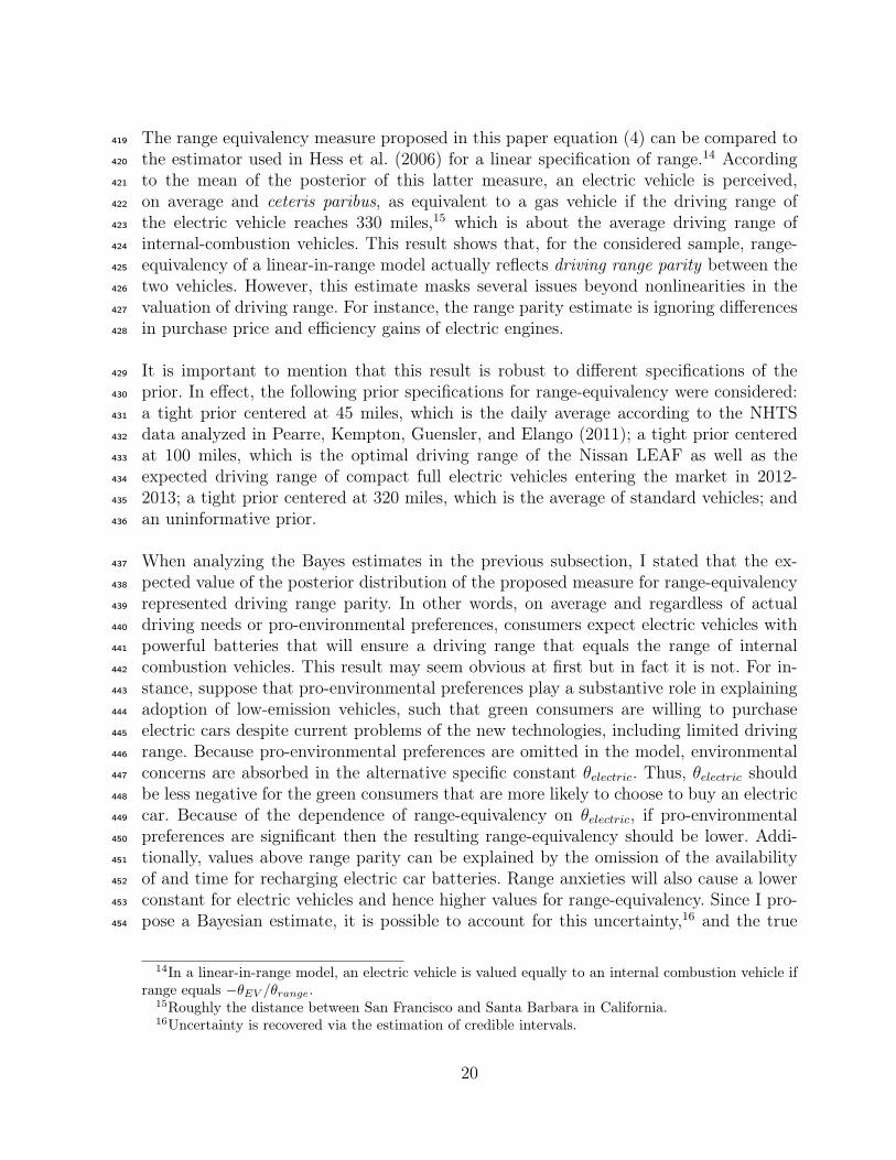
The range equivalency measure proposed in this paper equation (4) can be compared to419

the estimator used in Hess et al. (2006) for a linear specification of range.14 According420

to the mean of the posterior of this latter measure, an electric vehicle is perceived,421

on average and ceteris paribus, as equivalent to a gas vehicle if the driving range of422

the electric vehicle reaches 330 miles,15 which is about the average driving range of423

internal-combustion vehicles. This result shows that, for the considered sample, range-424

equivalency of a linear-in-range model actually reflects driving range parity between the425

two vehicles. However, this estimate masks several issues beyond nonlinearities in the426

valuation of driving range. For instance, the range parity estimate is ignoring differences427

in purchase price and efficiency gains of electric engines.428

It is important to mention that this result is robust to different specifications of the429

prior. In effect, the following prior specifications for range-equivalency were considered:430

a tight prior centered at 45 miles, which is the daily average according to the NHTS431

data analyzed in Pearre, Kempton, Guensler, and Elango (2011); a tight prior centered432

at 100 miles, which is the optimal driving range of the Nissan LEAF as well as the433

expected driving range of compact full electric vehicles entering the market in 2012-434

2013; a tight prior centered at 320 miles, which is the average of standard vehicles; and435

an uninformative prior.436

When analyzing the Bayes estimates in the previous subsection, I stated that the ex-437

pected value of the posterior distribution of the proposed measure for range-equivalency438

represented driving range parity. In other words, on average and regardless of actual439

driving needs or pro-environmental preferences, consumers expect electric vehicles with440

powerful batteries that will ensure a driving range that equals the range of internal441

combustion vehicles. This result may seem obvious at first but in fact it is not. For in-442

stance, suppose that pro-environmental preferences play a substantive role in explaining443

adoption of low-emission vehicles, such that green consumers are willing to purchase444

electric cars despite current problems of the new technologies, including limited driving445

range. Because pro-environmental preferences are omitted in the model, environmental446

concerns are absorbed in the alternative specific constant θelectric. Thus, θelectric should447

be less negative for the green consumers that are more likely to choose to buy an electric448

car. Because of the dependence of range-equivalency on θelectric, if pro-environmental449

preferences are significant then the resulting range-equivalency should be lower. Addi-450

tionally, values above range parity can be explained by the omission of the availability451

of and time for recharging electric car batteries. Range anxieties will also cause a lower452

constant for electric vehicles and hence higher values for range-equivalency. Since I pro-453

pose a Bayesian estimate, it is possible to account for this uncertainty,16 and the true454

14In a linear-in-range model, an electric vehicle is valued equally to an internal combustion vehicle ifrange equals −θEV /θrange.

15Roughly the distance between San Francisco and Santa Barbara in California.16Uncertainty is recovered via the estimation of credible intervals.

20

range-equivalency has a distribution around range parity.17455

5. Conclusions456

Electric vehicles currently offered in the market suffer from a rather limited driving range.457

This may be a major concern for consumers, who may be reluctant to convert to electric458

vehicles despite potential economies, as well as environmental benefits of such a decision.459

In this paper I have derived and studied the statistical behavior of three functions of460

the posterior distribution of the parameters of a vehicle choice model that are useful461

in understanding consumer concerns toward limited driving range of electric vehicles.462

The first function is the range-equivalency between an electric vehicle and a benchmark463

car, such as a standard gas vehicle or a hybrid. This range-equivalency measures the464

driving range level for which a consumer would perceive the electric vehicle and the465

benchmark car as being equally attractive, holding all other factors constant. The second466

function is the value of range, which is the marginal rate of substitution of driving range467

and purchase price. The third function is the capital-cost equivalency of range or the468

willingness to pay for improving the given driving range of an electric car in order to469

achieve range-equivalency with the benchmark car.470

The informative value of the proposed measures has been validated using stated prefer-471

ence data on vehicle choice in California. The data comprises behavioral purchase inten-472

tions of vehicles that are differentiated in several attributes, including energy source and473

driving range in the case of electric vehicles. A first result is that on average – and using474

gas vehicles as benchmark – consumers expect driving range parity between the electric475

and gas cars. This figure summarizes the importance of consumer preferences that may476

not reflect consumer needs. 78% of drivers commute 40 miles or less, which means that477

the currently offered range of 100 miles should suffice. However, consumers desire an478

electric battery with an average range of 330 miles. There are two aspects to keep in479

mind when analyzing this result. The range-equivalency of 330 miles is obtained focusing480

on range variations and holding all other attributes constant. This, of course, neglects481

the effect of transportation cost savings of electric cars. In addition, 330 miles is the482

expected value of the posterior distribution of range-equivalency. Since I have adopted483

a Bayesian approach for the estimation problem, the true parameters (and transforma-484

tions of the parameters of the model) are viewed as random variables. In the specific485

case of range-equivalency, this randomness accounts for uncertainty in the true value486

of the measure due to effects such as pro-environmental preferences and availability of487

recharging infrastructure, which are omitted in the experiment.488

17The introduction of pro-environmental preferences as a latent attitude (Daziano and Bolduc, 2011),as well as other causal interactions to explain the recovered uncertainty (including deterministic tastevariations and latent classes), should produce a narrower credible interval for the driving-range measures.

21

When operating cost savings are accounted for, range-equivalency does not reflect range489

parity. Consumers valuate positively that electric cars use a cheaper energy source, and490

purchase decisions reflect tradeoffs among these economies, higher purchase prices, and491

limited driving range. This positive valuation reduces range-equivalency which no longer492

reflects driving range parity. Introducing transportation cost savings and keeping all493

other attributes constant, consumers are willing to buy an electric car instead of a494

standard gas vehicle if, on average, the electric driving range equals 114 miles. This is495

another very interesting result, since the current range of 100% electric cars is about496

100 miles. However, desired range increases to 283 miles if a hybrid car is considered as497

benchmark.498

For the obtained value of range, which on average equals 8,400 US$ per additional 100499

miles, I have derived the posterior distribution of capital-cost equivalency of range. Be-500

cause operating cost reductions increase the overall utility of the consumer, there is a501

tradeoff among these benefits and drawbacks such as a high purchase price or limited502

driving range. The willingness to accept a higher purchase price in exchange for ex-503

pected lower monthly expenses, is an interesting measure that can also be interpreted as504

compensating price reductions. Integrating the operating cost savings, the average pur-505

chase price reduction that makes an electric vehicle with limited driving range equally506

attractive to a standard gas vehicle is 1,259 US$. The average purchase price reduction507

increases to 14,970 US$ when the comparison is made with respect to a hybrid car. That508

means that a consumer that is considering purchasing a hybrid vehicle should be offered509

14,970 US$ to ensure indifference between the hybrid vehicle and an electric car with a510

driving range limited to 100 miles. Looking at the results it is possible to conclude that511

hybrid vehicles may become the strongest competitor preventing the adoption of electric512

vehicles. Hybrid vehicles offer the best of both worlds: higher efficiency and environmen-513

tal benefits without a limiting driving range. Thus, to assess the potential success of514

the electric car, a deeper comparison has to be made with what appears as its strongest515

competitors: the plug-in hybrid and the extended range electric vehicle. Future empiri-516

cal research should focus in this comparison via the combination of stated and revealed517

preference data, to avoid any potential bias due to the gap between purchase intentions518

and actual behavior.519

Finally, this paper also contains technical contributions. When using frequentist meth-520

ods, one finds point estimates for the proposed measures that are an asymptotic ap-521

proximation of the Bayes point estimates. Not only are the Bayes estimators exact, but522

in addition – and as a direct result of the estimation procedure – one finds the poste-523

rior distribution of the measures of interest. Since the taste parameters have no direct524

interpretation, I have proposed to analyze the behavior of the posterior distributions525

of meaningful functions of the original parameters. Using the posterior distributions of526

range-equivalency, value of range, and capital-cost equivalency of range, I have shown527

and compared the performance of two transition processes for Metropolis-Hastings esti-528

mation of a conditional logit model for low-emission-vehicle choice. In addition, a slice529

22

sampling estimator, which is a special case of a Gibbs sampler, was also tested. As ex-530

pected, independence Metropolis Hastings performs better than a random walk, which531

introduces high posterior autocorrelations, and better than slice sampling, which has532

autocorrelation and longer estimation times because of the need to take draws from533

truncated distributions.534

References535

M. Achtnicht. German car buyers’ willingness to pay to reduce co2 emissions. Climatic Change,536

113(3):679–697, 2012.537

S. Beggs, S. Cardell, and J. Hausman. Assessing the potential demand for electric cars. Journal538

of Econometrics, 17(1):1 – 19, 1981.539

Steven D. Beggs and N.Scott Cardell. Choice of smallest car by multi-vehicle households and540

the demand for electric vehicles. Transportation Research Part A: General, 14(5–6):389 –541

404, 1980.542

D. Bolduc, L. Khalaf, and C. Yélou. Identification robust confidence set methods for inference543

on parameter ratios with application to discrete choice models. Journal of Econometrics, 157544

(2):317 – 327, 2010.545

D. Brownstone, D.S. Bunch, and K. Train. Joint mixed logit models of stated and revealed546

preferences for alternative-fuel vehicles. Transportation Research Part B: Methodological, 34547

(5):315 – 338, 2000.548

D.S. Bunch, M. Bradley, T.F. Golob, R. Kitamura, and G.P. Occhiuzzo. Demand for clean-549

fuel vehicles in california: A discrete-choice stated preference pilot project. Transportation550

Research Part A: Policy and Practice, 27(3):237 – 253, 1993.551

J.E. Calfee. Estimating the demand for electric automobiles using fully disaggregated proba-552

bilistic choice analysis. Transportation Research Part B, 19:287–301, 1985.553

S. Chib, E. Greenberg, and Y. Chen. MCMC methods for fitting and comparing multinomial554

response models. Econometrics 9802001, EconWPA, Feb 1998.555

P. Damien, J. Wakefield, and S. Walker. Gibbs sampling for bayesian non-conjugate and hier-556

archical models by using auxiliary variables. Journal of the Royal Statistical Society, 61(2):557

331–344, 1999.558

R.A. Daziano and D. Bolduc. Incorporating pro-environmental preferences towards green auto-559

mobile technologies through a Bayesian hybrid choice model. Transportmetrica, 2011. URL560

http://www.informaworld.com/10.1080/18128602.2010.524173.561

R.A. Daziano and E. Chiew. Electric vehicles rising from the dead: Data needs for forecasting562

consumer response toward sustainable energy sources in personal transportation. Energy563

Policy, 2012. doi: 10.1016/j.enpol.2012.09.040.564

A. Dimitropoulos, P. Rietveld, and J. N. van Ommeren. Consumer valuation of driving range:565

a meta-analysis. Working paper, Tinbergen Institute, 2012.566

G.O. Ewing and Sarigöllü. Car fuel-type choice under travel demand management and economic567

incentives. Transportation Research Part D, 3(6):429–444, 1998.568

S. Frühwirth-Schnatter and R. Frühwirth. Data augmentation and mcmc for binary and multi-569

nomial logit models. In Thomas Kneib and Gerhard Tutz, editors, Statistical Modelling and570

Regression Structures, pages 111–132. Physica-Verlag HD, 2010.571

23

General Motors. GM US deliveries for December 2010, January 2011, and February 2011, 2011.572

URL http://media.gm.com/media/us/en/news.html/.573

J. Geweke. Evaluating the accuracy of sampling-based approaches to the calculation of posterior574

moments (with discussion). In J.M. Bernardo, J.O. Berger, A.P. Dawid, and A.F.M Smith,575

editors, Bayesian Statistics 4, pages 169–193. Oxford University Press, 1992.576

T.F. Golob, J. Torous, M. Bradley, D. Brownstone, S.S. Crane, and D.S. Bunch. Commercial577

fleet demand for alternative-fuel vehicles in california. Transportation Research Part A, 31:578

219–233, 1997.579

S. Hess, K.E. Train, and J.W. Polak. On the use of a modified latin hypercube sampling580

(MLHS) method in the estimation of a mixed logit model for vehicle choice. Transportation581

Research Part B, 40:147 – 163, 2006.582

S. Hess, M. Fowler, T. Adler, and A. Bahreinian. A joint model for vehicle type and fuel type583

choice: evidence from a cross-nested logit study. Transportation, 39(3):593–625, 2012.584

M.K. Hidrue, G.R. Parsons, W. Kempton, and M.P. Gardner. Willingness to pay for electric585

vehicles and their attributes. Resource and Energy Economics, 33(3):686 – 705, 2011.586

C. Kavalec. Vehicle choice in an aging population: some insights from a stated preference survey587

for california. The Energy Journal, 20(3):123–138, 1999.588

G. Koop and D.J. Poirier. Bayesian analysis of logit models using natural conjugate priors.589

Journal of Econometrics, 56(3):323 – 340, 1993.590

D. McFadden. Conditional logit analysis of qualitative choice behavior. In P. Zarembka, editor,591

Frontier in Econometrics. Academic Press, New York, NY, 1974.592

D. McFadden and K.E. Train. Mixed MNL models of discrete response. Journal of Applied593

Econometrics, 15:447 – 470, 2000.594

National Automobile Dealers Association. NADA DATA Report. 2010.595

R.M. Neal. Slice sampling. Annals of Statistics, 3:705–767, 2003.596

Nissan. NNA December, January and February sales, 2011. URL597

http://www.nissannews.com/.598

H. Nixon and J.D. Saphores. Understanding household preferences for alternatives-fuel vehicle599

technologies. Report 10-11, Mineta Transportation Institute, San José, CA, 2011.600

Nathaniel S. Pearre, Willett Kempton, Randall L. Guensler, and Vetri V. Elango. Electric601

vehicles: How much range is required for a day’s driving? Transportation Research Part C:602

Emerging Technologies, 19(6):1171 – 1184, 2011.603

A.E. Raftery and S.M. Lewis. One long run with diagnostics: Implementation strategies for604

Markov chain Monte Carlo. Statistical Science, 7:493–497, 1992.605

P.E. Rossi, G.M. Allenby, and R. McCulloch. Bayesian Statistics and Marketing. John Wiley606

& Sons, Chichester, West Sussex, UK, 2005.607

Z. Sándor and K. Train. Quasi-random simulation of discrete choice models. Transportation608

Research Part B, 38(4):313 – 327, 2004.609

S. Scott. Data augmentation for the bayesian analysis of multinomial logit models. Proceedings,610

American Statistical Association Section on Bayesian Statistical Science, Alexandria, VA,611

2003.612

S. Scott. Data augmentation, frequentist estimation, and the bayesian analysis of multi-613

nomial logit models. Statistical Papers, 52:87–109, 2011. ISSN 0932-5026. URL614

http://dx.doi.org/10.1007/s00362-009-0205-0. 10.1007/s00362-009-0205-0.615

Garrett Sonnier, Andrew Ainslie, and Thomas Otter. Heterogeneity distributions of willingness-616

24

to-pay in choice models. Quantitative Marketing and Economics, 5:313–331, 2007.617

M. Tompkins, D.S. Bunch, D. Santini, M. Bradley, A. Vyas, and D. Poyer. Determinants618

of alternative fuel vehicle choice in the continental united states. Transportation Research619

Record, 1641:130–138, 1998.620

K. Train and K. Hudson. The impact of information in vehicle choice and the demand for621

electric vehicles in California. Project report, National Economic Research Associates, 2000.622

K. Train and G. Sonnier. Mixed logit with bounded distributions of correlated partworths. In623

R. Scarpa and A. Alberini, editors, Applications of Simulation Methods in Environmental624

and Resource Economics. Kluwer Academic Publishers, Boston, MA, 2005.625

US Department of Transportation. Summary of fuel economy performance, 2010. URL626

http://www.nhtsa.gov/.627

US Department of Transportation. 2009 National Household Travel Survey, 2011. URL628

http://nhts.ornl.gov.629

US Environmenal Protection Agency. Alternative fuel conversion, 2011. URL630

http://www.epa.gov/otaq/consumer/fuels/altfuels/altfuels.htm.631

J.C. Wakefield, A.E. Gelfand, and A.F.M. Smith. Efficient generation of random variates via632

the ratio-of-uniforms method. Statistics and Computing, 1:129–133, 1991.633

Appendix A. Bayes estimators of the conditional logit model634

Appendix A.1. Fixed parameter logit635

Consider a standard choice situation where for each individual n ∈ {1, ..., N} an exoge-636

nous random sample contains independent choice indicators yin for each discrete alterna-637

tive i in the set Cn.18 The choice indicator yin identifies whether alternative i was chosen638

by individual n or not. This observed choice is the base of a revealed-preference mecha-639

nism that manifests an underlying truncated indirect utility function Uin = x′inθ + εin,640

where xin is a vector of attributes or constituent characteristics of the discrete alter-641

natives, θ is a vector of unknown parameters representing consumer tastes, and εin is642

an error term.19 The link between the binary observations yin and the indirect utility643

function is given by the measurement equation yin = 1 if Uin = maxj∈Cn Ujn. Under the644

assumption εiniid∼ EV1(0, λ), the parametric model that generates the data is such that645

Pin =exp(λ−1x′inθ)∑

j∈Cn

exp(λ−1x′jnθ), (A.1)

where Pin are the choice probabilities derived from the model. For identification of θ it646

is necessary to normalize the scale of utility λ = 1.647

18Cn contains a total of Jn available alternatives.19I.e. a random parametric linear specification is assumed for the indirect utility function.

25

Since the elements yn|Xn in the sample space20 and the choice probabilities in equation648

A.1 define a dominated parametric conditional model, frequentist point estimation is649

based on maximizing the likelihood650

`(θ;y|X) =N∏n=1

Jn∏i=1

exp(x′inθ)∑j∈Cn

exp(x′jnθ)

yin

. (A.2)

In a Bayesian context, the parameters θ of the model are assumed to have a prior dis-651

tribution p(θ) that describes the probability distribution of θ before the observation of652

the sample data y|X. Considering θ to be a random variable is what distinguishes the653

Bayesian approach from frequentist statistics. This notion is fundamental for Bayesian654

inference and is derived from the concept of subjective probabilities.21 The combination655

of the prior distribution p(θ) with the information coming in via the sample determines656

the posterior distribution of the parameters p(θ|y,X). The posterior and prior distribu-657

tions are related following Bayes’ theorem according to658

p(θ|y,X) =`(θ;y|X)p(θ)

p(y|X),

where p(y|X) is the distribution of the data. For inference purposes Bayes’ theorem is659

rewritten as p(θ|y,X) ∝ `(θ;y|X)p(θ) or660

p(θ|y,X) ∝ p(θ)N∏n=1

Jn∏i=1

exp(x′inθ)∑j∈Cn

exp(x′jnθ)

yin

, (A.3)

an expression that emphasizes the Bayesian notion of updating knowledge through evi-661

dence.662

Even though Bayesian inference is focused on the posterior distribution p(θ|y,X), the663

calculation of the first and second moments of the posterior are of fundamental interest.664

In fact, the posterior mean θ̂ = E(θ|y,X) is the Bayes decision for the point estima-665

tion problem that minimizes the Bayes risk with a quadratic loss function. And with a666

quadratic loss function, the posterior variance E[var(θ|y,X)] is an unbiased estimator667

of the precision of the Bayes decision θ̂ = E(θ|y,X).668

An important class of Bayes estimators use conjugate distributions, for which both the669

20yn = (y1n, ..., yJnn)′, Xn = (x′

1n, ...,x′Jnn

).21Subjective probabilities measure the beliefs about the occurrence of a particular event.

26

posterior and the prior belong to the same family of distributions.22 In the case of the con-670

ditional logit model, however, there is no general conjugate prior (cf. Koop and Poirier,671

1993). When this occurs, a Bayes estimator can be derived using the iterative Metropolis-672

Hastings algorithm.23 Let Θ be the parameter space. Using Metropolis-Hastings, a can-673

didate θcand ∈ Θ is drawn from the transition probability q(θcand|θcurr) of generating674

candidate θcand given θcurr ∈ Θ, such that θcurr ∼ p(θ,y|X). The candidate realization675

θcand is then compared to the current θcurr ∈ Θ through the acceptance ratio:676

α = min

{1,`(θcand;y|X)p(θcand)q(θcand|θcurr)`(θcurr;y|X)p(θcurr)q(θcurr|θcand)

}. (A.4)

Starting with an arbitrary value θ(0), at the gth iteration of the Metropolis-Hastings677

algorithm the candidate is accepted as the new θ(g) = θcand with probability α, whereas678

the old one is preserved θ(g) = θcurr with probability 1− α.679

Consider the following asymptotic approximation to the posterior distribution of the680

conditional logit model (Scott, 2003):681

p(θ|y,X) ∝ |I(θ)|12 exp

(1

2(θ − θ̂MLE)′I(θ)(θ − θ̂MLE)

), (A.5)

where θ̂MLE is the maximum likelihood estimator of θ, i.e. the value θ̂ML(y|X) that682

maximizes the likelihood function `(θ;y|X) once y is observed, and where I(θ) is the683

Fisher information matrix of the conditional logit model.24684

Based on the asymptotic approximation to the posterior in equation A.4, Rossi et al.685

(2005) propose two transition processes for updating θ in the Metropolis-Hastings al-686

gorithm. For a random-walk Metropolis chain, the candidate realization is defined as687

θcand = θcurr + ε, where ε ∼ N (0, s2I−1) and s2 is the precision. For an independence688

Metropolis, the candidate realization is found using θcand ∼ MSt(ν, θ̂MLE, I−1), i.e.689

θcand is drawn from a multivariate t distribution with mean θ̂MLE, dispersion I−1, and690

ν degrees of freedom.25691

Consider p(θ) ∼ N (b̌, B̌−1), a multivariate normal prior on θ with mean b̌ and precision692

22In the case of conjugate distributions, inference is based on direct sampling from the known para-metric form of the posterior.

23Metropolis-Hastings belongs to the class of Markov chain Monte Carlo (MCMC) methods, which arestochastic sampling algorithms based on constructing a Markov chain that has the posterior distributionas its equilibrium distribution. The estimators are based on numerical approximations from posteriorsimulators.

24Instead of considering the maximum likelihood estimator, the approximation A.4 can also be eval-uated at the posterior mode (Chib et al., 1998).

25This is a generalization of the estimator proposed by Chib et al. (1998).

27

B̌. To include the effect of the prior precision it is possible to extend both transition693

processes. Thus, it is possible to consider the following general transition process θcand ∼694

N (θcurr,S[B̌ + I(θ̂MLE)]−1]S) for the random walk, and θcand ∼ MSt(ν, θ̂MLE,S[B̌ +695

I(θ̂MLE)]−1S) for independence Metropolis-Hastings, where S is a diagonal matrix with696

elements that adjust the covariance matrix of the candidate to get satisfactory acceptance697

ratios. The implication here is that both S and ν work as tuning parameters.698

I will discuss now the implementation of the slice sampler (Wakefield, Gelfand, and699

Smith, 1991, Damien, Wakefield, and Walker, 1999, Neal, 2003), which is a special case700

of the Metropolis-Hasting algorithm.26 The slice sampler exploits data augmentation701

methods, where auxiliary variables are summed up to the parameter space in order to702

get full conditional distributions of standard form while keeping the marginal posterior703

of interest. Consider the posterior (A.3) of the conditional logit model, which depends704

on the choice probabilities through the likelihood function as well as on the prior. When705

introducing the auxiliary variables of the slice sampler, the likelihood function can be706

rewritten as an associated completion where the choice probabilities truncate the pa-707

rameter space to reflect information summarized by the choice indicators. Then, with a708

normally distributed prior, the posterior can be simulated from a truncated multivariate709

normal distribution. An attractive feature of the slice sampler is that it does not require710

tuning.711

In effect, consider a Bayesian conditional logit model as in equation A.1 with prior p(θ) ∼712

N (b̌, B̌−1). Note that the choice probabilities Pin = P (εjn − εin < (xin − xjn)′θ,∀j 6=713

i ∈ Cn) are given by the cumulative distribution of a logistic.27714

In the specific case of binary choice, and labeling by i and j the two available alternatives,715

the choice probability of alternative i is Pin = P (εjn − εin < (xin − xjn)′θ). Even716

though it is possible to write a similar expression for Pjn, note that in the binary case717

Pjn = 1 − Pin. Since the difference εjn − εin for a normalized model has a standard718

logistic distribution, then Pin = E(yin|xin) = Λ[(xin − xjn)′θ], where Λ[(xin − xjn)′θ] =719

exp((xin − xjn)′θ)/(1 + exp((xin − xjn)′θ)). Because Pjn = 1/(1 + exp((xin − xjn)′θ)),720

then the posterior takes the form721

p(θ|y,X) ∝ p(θ)N∏n=1

[exp((xin − xjn)′θ)

1 + exp((xin − xjn)′θ)

]yin [ 1

1 + exp((xin − xjn)′θ)

]yin−1

. (A.6)

26The slice sampler is a subclass of Gibbs sampling. A Gibbs sampler approximates the joint posteriorby sampling from a conditional decomposition of the posterior.

27The choice probability of a conditional logit model depends on the difference of two random termsEV1(0, 1), which has a logistic distribution.

28

Consider now the following uniform auxiliary variable722

un ∼ U

(0,

exp(yin(xin − xjn)′θ)

1 + exp((xin − xjn)′θ)

), (A.7)

where the logit expression has been conveniently rewritten to summarize both Pin and723

Pjn.724

Using the auxiliary variable un, the posterior (A.6) becomes725

p(θ|y,X) ∝ p(θ)N∏n=1

Iun≤

exp(yin(xin−xjn)′θ)

1+exp((xin−xjn)′θ)

, (A.8)

where I is an indicator function.726

Thus, the slice sampling estimator is built from iterative draws inside a Gibbs sampler,727

which at the gth iteration considers728

u(g)n ∼ U

(0,

exp(yin(xin − xjn)′θ(g))

1 + exp((xin − xjn)′θ(g))

),∀n

θ(g+1) ∼ N (b̌, B̌−1)N∏n=1

Iu

(g)n ≤

exp(yin(xin−xjn)′θ(g))

1+exp((xin−xjn)′θ(g))

,

i.e. θ is simulated from a multidimensional truncated normal distribution.729

If B̌ is assumed to be diagonal, then element θk is simulated from730

θ(g+1)k ∼ N (θ̌k, σ̌

2k)

N∏n=1

Iu

(g)n ≤

exp(yin(xin−xjn)′θ(g))

1+exp((xin−xjn)′θ(g))

, (A.9)

where θ̌k and σ̌2k are hyperparameters of the normally distributed prior. Note that the731

conditional distribution of θk depends on the vectors θ(g+1)′

<k = (θ(g+1)′

1 , ..., θ(g+1)′

k−1 ) and732

θ(g)′

>k = (θ(g)′

k+1, ..., θ(g)′

K ), which are both implicitly summarized by θ(g).733

The truncation region is defined by the choice indicator. If yin = 1, then un ≤ Λ[(xin −734

xjn)′θ] which can be inverted into (xin − xjn)′θ ≥ ln(un/(1 − un)). If yin = 0, then735

un ≤ − ln(un/(1− un)). Then, the truncation region can be summarized as736

N⋂n=1

{θ : (−1)yin(xin − xjn)′θ ≥ ln

un1− un

}(A.10)

29

For each parameter, the truncation region (A.10) yields the following thresholds737

θk = maxn:yin=1

{(xkin − xkjn)−1

(ln

un1− un

− (xin − xjn)′θ\k

)}θ̄k = min

n:yin=1

{(xkin − xkjn)−1

(ln

1− unun

− (xin − xjn)′θ\k

)}where θk ≤ θk ≤ θ̄k and θ\k = (θ1, ..., θk−1, 0, θk+1, ..., θK)′. Then, in the slice sampler it738

is possible to consider θk ∼ Nθk≤θk≤θ̄k(θ̌k, σ̌2k). This is the procedure that Winbugs uses739

for sampling the parameters of a binary logit.740

The method can be easily extended to accommodate multinomial choice.741

Appendix A.2. Random parameter logit742

A solution to the problem of repeated observations is found by adopting the Markov chain743

Monte Carlo sampler of a hierarchical conditional logit model with random parameters744

(Train and Sonnier, 2005).745

Appendix B. Choice Situation Sample746

30

Figure B.5: Sample of a choice situation presented to respondents of the stated preference experiment.Source: Train and Hudson (2000).

31