arX

iv:0

803.

3753

v2 [

mat

h.PR

] 2

8 A

ug 2

009

The Annals of Probability

2009, Vol. 37, No. 4, 1566–1586DOI: 10.1214/08-AOP443c© Institute of Mathematical Statistics, 2009

CONDITIONAL HAAR MEASURES ON CLASSICAL

COMPACT GROUPS

By P. Bourgade

Universite Paris 6

We give a probabilistic proof of the Weyl integration formula onU(n), the unitary group with dimension n. This relies on a suitabledefinition of Haar measures conditioned to the existence of a stablesubspace with any given dimension p. The developed method leadsto the following result: for this conditional measure, writing Z

(p)U for

the first nonzero derivative of the characteristic polynomial at 1,

Z(p)U

p!

law=

n−p∏

ℓ=1

(1−Xℓ),

the Xℓ’s being explicit independent random variables. This implies acentral limit theorem for logZ

(p)U and asymptotics for the density of

Z(p)U near 0. Similar limit theorems are given for the orthogonal and

symplectic groups, relying on results of Killip and Nenciu.

1. Introduction, statements of results. Let µU(n) be the Haar measureon U(n), the unitary group over C

n. By the Weyl integration formula, forany continuous class function f ,

EµU(n)(f(u))

(1.1)

=1

n!

∫

· · ·∫

|∆(eiθ1 , . . . , eiθn)|2f(eiθ1, . . . , eiθn)dθ1

2π· · · dθn

2π,

where ∆ denotes the Vandermonde determinant. Classical proofs of thisdensity of the eigenvalues make use of the theory of Lie groups (see, e.g.,[6]), raising the question of a more probabilistic proof of it.

Problem 1. Can we give a probabilistic proof of (1.1)?

Received April 2008; revised August 2008.AMS 2000 subject classifications. 15A52, 60F05, 14G10.Key words and phrases. Random matrices, characteristic polynomial, the Weyl integra-

tion formula, zeta and L-functions, central limit theorem.

This is an electronic reprint of the original article published by theInstitute of Mathematical Statistics in The Annals of Probability,2009, Vol. 37, No. 4, 1566–1586. This reprint differs from the original inpagination and typographic detail.

1

2 P. BOURGADE

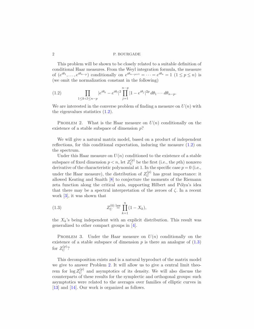
This problem will be shown to be closely related to a suitable definition ofconditional Haar measures. From the Weyl integration formula, the measureof (eiθ1 , . . . , eiθn−p) conditionally on eiθn−p+1 = · · · = eiθn = 1 (1 ≤ p ≤ n) is(we omit the normalization constant in the following)

∏

1≤k<l≤n−p

|eiθk − eiθl |2n−p∏

j=1

|1− eiθj |2p dθ1 · · · dθn−p.(1.2)

We are interested in the converse problem of finding a measure on U(n) withthe eigenvalues statistics (1.2).

Problem 2. What is the Haar measure on U(n) conditionally on theexistence of a stable subspace of dimension p?

We will give a natural matrix model, based on a product of independentreflections, for this conditional expectation, inducing the measure (1.2) onthe spectrum.

Under this Haar measure on U(n) conditioned to the existence of a stable

subspace of fixed dimension p < n, let Z(p)U be the first (i.e., the pth) nonzero

derivative of the characteristic polynomial at 1. In the specific case p = 0 (i.e.,

under the Haar measure), the distribution of Z(p)U has great importance: it

allowed Keating and Snaith [8] to conjecture the moments of the Riemannzeta function along the critical axis, supporting Hilbert and Polya’s ideathat there may be a spectral interpretation of the zeroes of ζ . In a recentwork [3], it was shown that

Z(0)U

law=

n∏

k=1

(1−Xk),(1.3)

the Xk’s being independent with an explicit distribution. This result wasgeneralized to other compact groups in [4].

Problem 3. Under the Haar measure on U(n) conditionally on theexistence of a stable subspace of dimension p is there an analogue of (1.3)

for Z(p)U ?

This decomposition exists and is a natural byproduct of the matrix modelwe give to answer Problem 2. It will allow us to give a central limit theo-

rem for logZ(p)U and asymptotics of its density. We will also discuss the

counterparts of these results for the symplectic and orthogonal groups: suchasymptotics were related to the averages over families of elliptic curves in[13] and [14]. Our work is organized as follows.

CONDITIONAL HAAR MEASURES 3

Conditional Haar measures. Let (e1, . . . , en) be an orthonormal basis ofC

n, and r(k) (1 ≤ k ≤ n) independent reflections in U(n) (i.e., Id− r(k) hasrank 0 or 1). Suppose that r(k)(ej) = ej for 1≤ j ≤ k− 1 and that r(k)(ek) isuniformly distributed on the complex sphere {(0, . . . ,0, xk, . . . , xn) | |xk|2 +· · ·+ |xn|2 = 1}. Results from [3] and [4] state that

r(1) · · · r(n)

is Haar-distributed on U(n). We generalize this in Section 2, showing that

r(1) · · · r(n−p)(1.4)

properly defines the Haar measure on U(n) conditioned to the existence ofa stable subspace of dimension p.

A probabilistic proof of the Weyl integration formula. The previous con-ditioning of Haar measures allows to derive the Weyl integration formula(1.1) by induction on the dimension, as explained in Section 3. Our proofrelies on an identity in law derived in the Appendix. As a corollary, wedirectly show that the random matrix (1.4) has the expected spectral law(1.2).

The derivatives as products of independent random variables. For theconditional Haar measure from Section 1 [µU(n) conditioned to the exis-tence of a stable subspace of dimension p], we show that the first nonzeroderivative of the characteristic polynomial is equal in law to a product ofn− p independent random variables:

Z(p)U

p!law=

n−p∏

ℓ=1

(1−Xℓ).(1.5)

This is a direct consequence of the decomposition (1.4). The analogous resultfor orthogonal and symplectic groups will be stated, directly relying on aprevious work by Killip and Nenciu [9] about orthogonal polynomials onthe unit circle (OPUC) and the law of the associated Verblunsky coefficientsunder Haar measure. Links between the theory of OPUC and reflections willbe developed in a forthcoming paper [5].

Limit theorems for the derivatives. The central limit theorem proved byKeating and Snaith [8], and first conjectured by Costin and Lebowitz [7],

gives the asymptotic distribution of logZ(0)U . More precisely, the complex

logarithm of det(Id − xu) being continuously defined along x ∈ (0,1), theyshowed that

logZ(0)U

√

1/2 log n

law−→N1 + iN2(1.6)

4 P. BOURGADE

as n → ∞ with N1 and N2 independent standard normal variables. Theanalogue of their central limit theorem for the Riemann zeta function waspreviously known by Selberg [12] and can be stated as

1

T

∫ T

0dt1( log ζ(1/2 + it)

√

1/2 log logT∈ Γ

)T→∞−→

∫ ∫

Γ

dxdy

2πe−(x2+y2)/2

for any regular Borel set Γ in C. Section 4 explains how the identity in law(1.5) allows to generalize (1.6):

logZ(p)U − p logn

√

1/2 log n

law−→N1 + iN2.

From results in [9], a similar central limit theorem holds for the orthogonaland symplectic groups, jointly for the first nonzero derivative at 1 and −1.This will be related to works by Snaith ([13] and [14]) in number theory;

her interest is in the asymptotic density of Z(2p)SO

near 0. Using identities inlaw such as (1.5), we give such density asymptotics for the classical compactgroups.

2. Conditional Haar measure. For r a n × n complex matrix, the sub-script rij stands for 〈ei, r(ej)〉, where 〈x, y〉 =

∑nk=1 xkyk.

2.1. Reflections. Many distinct definitions of reflections on the unitarygroup exist, the most well known may be the Householder reflections. Thetransformations we need in this work are the following.

Definition 2.1. An element r in U(n) will be referred to as a reflectionif r − Id has rank 0 or 1.

The reflections can also be described in the following way. Let M(n) bethe set of n× n complex matrices m that can be written

m =

(

m1, e2 − km12

1−m11, . . . , en − k

m1n

1−m11

)

(2.1)

with the vector m1 = (m11, . . . ,m1,n)⊤ 6= e1 on the n-dimensional unit com-plex sphere and k = m1 − e1. Then the reflections are exactly the elements

r =

(Idk−1 0

0 m

)

with m ∈ M(n − k + 1) for some 1 ≤ k ≤ n. For fixed k, the set of theseelements is noted R(k). If the first column of m, m1, is uniformly distributedon the unit complex sphere of dimension n− k + 1, it induces a measure onR(k), noted ν(k).

CONDITIONAL HAAR MEASURES 5

The nontrivial eigenvalue eiθ of a reflection r ∈R(k) is

eiθ = −1− rkk

1− rkk.(2.2)

A short proof of it comes from eiθ = Tr(r)− (n− 1). We see from (2.2) thatfor r ∼ ν(k) this eigenvalue is not uniformly distributed on the unit circle,and converges in law to −1 as n →∞.

2.2. Haar measure as the law of a product of independent reflections.The following two results are the starting point of this work: Theorems2.2 and 2.3 bellow will allow us to properly define the Haar measure onU(n) conditioned to have eigenvalues equal to 1. These results appear in [3]and [4], where their proofs can be found.

In the following we make use of this notation: if u1 ∼ µ(1) and u2 ∼ µ(2)

are elements in U(n), then µ1 × µ2 stands for the law of u1u2.

Theorem 2.2. Let µU(n) be the Haar measure on U(n). Then

µU(n) = ν(1) × · · · × ν(n).

Theorem 2.3. Take r(k) ∈R(k) (1≤ k ≤ n). Then

det(Id− r(1) · · · r(n)) =n∏

k=1

(1− r(k)kk ).

Remark. As noted in [3] and [4], a direct consequence of the two theo-

rems above is det(Id−u)law=∏n

k=1(1−r(k)kk ), where u ∼ µU(n) and r(k) ∼ ν(k),

all being independent. As r(k)kk is the first coordinate of a vector uniformly

distributed on the unit complex sphere of dimension n− k + 1, it is equal inlaw to eiθ

√B1,n−k, with θ uniform on (−π,π) and B a beta variable with the

indicated parameters. Consequently, with obvious notation for the followingindependent random variables,

det(Id− u)law=

n∏

k=1

(1− eiθk

√

B1,n−k).(2.3)

This relation will be useful in the proof of the Weyl integration formula, inthe next section.

2.3. Conditional Haar measure as the law of a product of independentreflections. What could be the conditional expectation of u ∼ µU(n), con-ditioned to have one eigenvalue at 1? As this conditioning is with respect toan event of measure 0, such a choice of conditional expectation is not trivial.

6 P. BOURGADE

As previously, suppose we generate the Haar measure as a product ofindependent reflections: u = r(1) · · · r(n). Since Id − r(k) has rank 1 a.s., ourconditional expectation will naturally be constructed as a product of n−1 ofthese reflections: the unitary matrix u has one eigenvalue eiθ = 1 if and only

if r(k) = Id for some 1≤ k ≤ n, which yields r(k)kk = 1. As r

(k)kk

law= eiθ

√B1,n−k,

with the previous notation, r(n)nn is more likely to be equal to 1 than any

other r(k)kk (1 ≤ k ≤ n− 1).

Consequently, a good definition for the conditional expectation of u ∼µU(n), conditioned to have one eigenvalue at 1, is r(1) · · ·r(n−1). This idea isformalized in the following way.

Proposition 2.4. Let Z(x) = det(x Id − u) and dx be the measure of|Z(1)| under Haar measure on U(n). There exists a continuous family ofprobability measures P (x) (0 ≤ x ≤ 2n) such that for any Borel subset Γ ofU(n)

µU(n)(Γ) =

∫ 2n

0P (x)(Γ)dx.(2.4)

Moreover P (0) = ν(1) × · · · × ν(n−1) necessarily.

Remark. The continuity of the probability measures is in the sense ofweak topology: the map

x 7→∫

U(n)f(ω)dP (x)(ω)(2.5)

is continuous for any bounded continuous function f on U(n).

Proof. We give an explicit expression of this conditional expectation,

thanks to Theorem 2.3. Take x > 0. If∏n−1

k=1 |1− r(k)kk |> x/2, then there are

two r(n)nn ’s on the unit circle such that

∏nk=1 |1− r

(k)kk | = x:

r(n)nn = exp

(

±2iarcsinx

2∏n−1

k=1 |1− r(k)kk |

)

.(2.6)

These two numbers will be denoted r+ et r−. We write ν± for the distributionof r±, the random matrix in R(n) equal to Idn−1 ⊕ r+ with probability 1/2,Idn−1 ⊕ r− with probability 1/2. We define the conditional expectation, forany bounded continuous function f , by

EµU(n)(f(u) | |Z(1)| = x) =

E(f(r(1) · · ·r(n−1)r±)1∏n−1

k=1|1−r

(k)kk

|>x/2)

E(1∏n−1

k=1|1−r

(k)kk

|>x/2)

,(2.7)

CONDITIONAL HAAR MEASURES 7

the expectations on the RHS being with respect to ν(1) × · · · × ν(n−1) ×ν±. For such a choice of the measures P (x) (x > 0), (2.4) holds thanks toTheorems 2.2 and 2.3. Moreover, these measures are continuous in x, andfrom (2.6) and (2.7) they converge to ν(1) × · · · × ν(n−1) as x → 0. Thecontinuity condition and formula (2.4) impose unicity for (P (x),0≤ x ≤ 2n).Consequently P (0) necessarily coincides with ν(1) × · · · × ν(n−1). �

For any 1 ≤ k ≤ n − 1, we can state some analogue of Proposition 2.4,conditioning now with respect to

(|Z(1)|, |Z ′(1)|, . . . , |Z(k−1)(1)|).(2.8)

This leads to the following definition of the conditional expectation, whichis the unique suitable choice preserving the continuity of measures withrespect to (2.8).

Definition 2.5. For any 1 ≤ p ≤ n− 1, ν(1) × · · · × ν(n−p) is called theHaar measure on U(n) conditioned to have p eigenvalues equal to 1.

Remark. The above discussion can be held for the orthogonal group:the Haar measure on O(n) conditioned to the existence of a stable subspaceof dimension p (0 ≤ p≤ n− 1) is

ν(1)R

× · · · × ν(n−p)R

,

where ν(k)R

is defined as the real analogue of ν(k): a reflection r is ν(k)R

-distributed if r(ek) has its first k − 1 coordinates equal to 0 and the othersare uniformly distributed on the real unit sphere.

More generally, we can define this conditional Haar measure for anycompact group generated by reflections, more precisely any compact groupchecking condition (R) in the sense of [4].

Take p = n− 1 in Definition 2.5: the distribution of the unique eigenangledistinct from 1 coincides with the distribution of the nontrivial eigenangleof a reflection r ∼ ν(1), that is to say from (2.2)

eiφ = −1− r11

1− r11

law= − 1− eiθ

√B1,n−1

1− e−iθ√

B1,n−1.

In particular, this eigenvalue is not uniformly distributed on the unit circle:it converges in law to −1 as n →∞. This agrees with the idea of repulsionof the eigenvalues: we make it more explicit with the following probabilisticproof of the Weyl integration formula.

8 P. BOURGADE

3. A probabilistic proof of the Weyl integration formula. The followingtwo lemmas play a key role in our proof of the Weyl integration formula:the first shows that the spectral measure on U(n) can be generated by n− 1reflections (instead of n) and the second one gives a transformation fromthis product of n− 1 reflections in U(n) to a product of n− 1 reflections inU(n− 1), preserving the spectrum.

In the following, usp= v means that the spectra of the matrices u and v

are equally distributed.

3.1. The conditioning lemma. Remember that the measures ν(k) (1 ≤k ≤ n) are supported on the set of reflections: the following lemma wouldnot be true by substituting our reflections with Householder transformations,for example.

Lemma 3.1. Take r(k) ∼ ν(k) (1 ≤ k ≤ n), θ uniform on (−π,π) andu ∼ µU(n), all being independent. Then

usp= eiθr(1) · · ·r(n−1).

Proof. From Proposition 2.4, the spectrum of r(1) · · · r(n−1) is equal inlaw to the spectrum of u conditioned to have one eigenvalue equal to 1.

Moreover, the Haar measure on U(n) is invariant by translation, in par-ticular by multiplication by eiφ Id, for any fixed φ: the distribution of thespectrum in invariant by rotation.

Consequently, the spectral distribution of u ∼ µU(n) can be realized bysuccessively conditioning to have one eigenvalue at 1 and then shifting by

an independent uniform eigenangle, that is to say usp= eiθr(1) · · · r(n−1), giving

the desired result. �

3.2. The slipping lemma. Take 1 ≤ k ≤ n and δ a complex number. We

first define a modification ν(k)δ of the measure ν(k) on the set of reflections

R(k). Let

exp(k)δ :

{

R(k) → R+,

r 7→ (1− rkk)δ(1− rkk)

δ.

Then ν(k)δ is defined as the exp

(k)δ -sampling of a measure ν(k) on R(k), in the

sense of the following definition.

Definition 3.2. Let (X,F , µ) be a probability space, and h :X 7→ R+

a measurable function with Eµ(h(x)) > 0. Then a measure µ′ is said to bethe h-sampling of µ if for all bounded measurable functions f

Eµ′(f(x)) =Eµ(f(x)h(x))

Eµ(h(x)).

CONDITIONAL HAAR MEASURES 9

For Re(δ) > −1/2, 0 < Eν(k)(exp(k)δ (r)) < ∞, so ν

(k)δ is properly defined.

Lemma 3.3. Let r(k) ∼ ν(k) (1 ≤ k ≤ n − 1) and r(k)1 ∼ ν

(k)1 (2 ≤ k ≤ n)

be n× n independent reflections. Then

r(1) · · ·r(n−1) sp= r

(2)1 · · · r(n)

1 .

Proof. We proceed by induction on n. For n = 2, take r ∼ ν(1). Con-sider the unitary change of variables

Φ :

(e1

e2

)

7→ 1

|1− r11|2 + |r12|2(

r12 −(1− r11)1− r11 r12

)(e1

e2

)

.(3.1)

In this new basis, r is diagonal with eigenvalues 1 and r11 − |r12|2/(1− r11),so we only need to check that this last random variable is equal in law tothe |1 − X|2-sampling of a random variable X uniform on the unit circle.This is a particular case of the identity in law given in Theorem A.1.

We now reproduce the above argument for general n > 2. Suppose theresult is true at rank n − 1. Take u ∼ µU(n), independent of all the otherrandom variables. Obviously,

r(1) · · ·r(n−1) sp= (u−1r(1)u)(u−1r(2) · · ·r(n−1)u).

As the uniform measure on the sphere is invariant by a unitary change ofbasis, by conditioning by (u, r(2), . . . , r(n−1)) we get

r(1) · · · r(n−1) sp= r(1)(u−1r(2) · · · r(n−1)u),

whose spectrum is equal in law (by induction) to the one of

r(1)(u−1r(3)1 · · · r(n)

1 u)sp= (ur(1)u−1)r

(3)1 · · ·r(n)

1sp= r(1)r

(3)1 · · ·r(n)

1 .

Consider now the change of basis Φ (3.1), extended to keep (e3, . . . , en)

invariant. As this transition matrix commutes with r(3)1 · · · r(n)

1 , to conclude

we only need to show that Φ(r(1))law= r

(2)1 . Both transformations are reflec-

tions, so a sufficient condition is Φ(r(1))(e2)law= r

(2)1 (e2). A simple calculation

gives

Φ(r(1))(e2) =

(

0, r11 −|r12|21− r11

, cr13, . . . , cr1n

)⊤,

where the constant c depends uniquely on r11 and r12. Hence the desiredresult is a direct consequence of the identity in law from Theorem A.1. �

Remark. The above method and the identity in law stated in TheoremA.1 can be used to prove the following more general version of the slipping

10 P. BOURGADE

lemma. Let 1 ≤ m ≤ n − 1, δ1, . . . , δm be complex numbers with real part

greater than −1/2. Let r(k)δk

∼ ν(k)δk

(1 ≤ k ≤ m) and r(k)δk−1+1 ∼ ν

(k)δk−1+1 (2 ≤

k ≤ m + 1) be independent n× n reflections. Then

r(1)δ1

· · · r(m)δm

sp= r

(2)δ1+1 · · · r

(m+1)δm+1 .

In particular, iterating the above result,

r(1) · · · r(n−p) sp= r(p+1)

p · · · r(n)p .(3.2)

Together with Theorem 2.3, this implies that the eigenvalues of r(1) · · ·r(n−p)

have density (1.2), as expected.

3.3. The proof by induction. The two previous lemmas give a recursiveproof of the following well-known result.

Theorem 3.4. Let f be a class function on U(n) :f(u) = f(θ1, . . . , θn),where the θ’s are the eigenangles of u and f is symmetric. Then

EµU(n)(f(u)) =

1

n!

∫

(−π,π)nf(θ1, . . . , θn)

∏

1≤k<l≤n

|eiθk − eiθl |2 dθ1

2π· · · dθn

2π.

Proof. We proceed by induction on n. The case n = 1 is obvious. Sup-pose the result holds at rank n− 1. Successively by the conditioning lemmaand the slipping lemma, if u ∼ µU(n),

usp= eiθr(1) · · · r(n−1) sp

= eiθr(2)1 · · ·r(n)

1 .

Hence, using the recurrence hypothesis, for any class function f ,

EµU(n)(f(u))

=1

cst

∫ π

−π

dθ

2π

1

(n− 1)!

×∫

(−π,π)n−1f(θ, θ2 + θ, . . . , θn + θ)

×∏

2≤k<l≤n

|eiθk − eiθl |2n∏

j=2

|1− eiθj |2 dθ2

2π· · · dθn

2π

=1

cst

1

(n− 1)!

∫

(−π,π)nf(θ1, . . . , θn)

∏

1≤k<l≤n

|eiθk − eiθl |2 dθ1

2π· · · dθn

2π.

Here cst comes from the sampling: cst = EµU(n−1)(|det(Id − u)|2). This is

equal to n from the decomposition of det(Id−u) into a product of indepen-dent random variables (2.3), which completes the proof. �

CONDITIONAL HAAR MEASURES 11

4. Derivatives as products of independent random variables. As ex-plained in [3] and [4], det(Id − u) is equal in law to a product of n inde-pendent random variables, for the Haar measure on U(n) or USp(2n), and2n independent random variables, for the Haar measure on SO(2n). Theseresults are generalized to the Haar measures conditioned to the existence ofa stable subspace with given dimension.

We first focus on the unitary group. Consider the conditional Haar mea-sure (1.2) on U(n) (θn−p+1 = · · · = θn = 0 a.s.). Then the pth derivative ofthe characteristic polynomial at 1 is

Z(p)U = p!

n−p∏

k=1

(1− eiθk).

Our discussion about Haar measure on U(n) conditioned to have a stable

subspace with dimension p allows us to decompose Z(p)U as a product of

independent random variables. More precisely, the following result holds.

Corollary 4.1. Under the conditional Haar measure (1.2),

Z(p)U

p!law=

n−p∏

ℓ=1

(1−Xℓ),

where the Xℓ’s are independent random variables. The distribution of Xℓ

is the |1 − X|2p-sampling of a random variable X = eiθ√

B1,ℓ−1, were θ isuniform on (−π,π) and independently B1,ℓ−1 is a beta variable with theindicated parameters.

Proof. This proof directly relies on the suitable Definition 2.5 of theconditional Haar measure: it does not make use of the Weyl integrationformula.

With the notation of Definition 2.5 (r(1) · · ·r(n−p) ∼ ν(1) × · · · × ν(n−p)),

Z(p)U

law=

dp

dxp x=1det(x Idn − r(1) · · · r(n−p)).

From (3.2), r(1) · · · r(n−p) sp= r

(p+1)p · · · r(n)

p , hence

Z(p)U

law=

dp

dxp x=1det(x Idn − r(p+1)

p · · · r(n)p ) = p!

n∏

k=p+1

(1− 〈ek, r(k)p (ek)〉),

the last equality being a consequence of Theorem 2.3. The r(k)p ’s are inde-

pendent and r(k)p ∼ ν

(k)p , which gives the desired result. �

12 P. BOURGADE

Remark. Another proof of the above corollary consists in using theWeyl integration formula and the generalized Ewens sampling formula givenin [4]. Actually, an identity similar to Corollary 4.1 can be stated for anyHua–Pickrell measure. More on these measures can be found in [2] for itsconnections with the theory of representations and in [4] for its analogieswith the Ewens measures on permutation groups.

Corollary 4.1 admits an analogue for the Jacobi ensemble on the segment.Indeed, Lemma 5.2 and Proposition 5.3 in [9], by Killip and Nenciu, imme-diately imply that under the probability measure (cst is the normalizationconstant)

cst|∆(x1, . . . , xn)|βn∏

j=1

(2− xj)a(2 + xj)

b dx1 · · · dxn(4.1)

on (−2,2)n, the following identity in law holds (the xk’s being the eigenvaluesof a matrix u):

(det(2 Id−u),det(2 Id+u))law=

(

22n−2∏

k=0

(1−αk),22n−2∏

k=0

(1+(−1)kαk)

)

,(4.2)

with the αk’s independent with density fs(k),t(k) (fs,t is defined below) on(−1,1) with

s(k) =2n− k − 2

4β + a + 1,

t(k) =2n− k − 2

4β + b + 1, if k is even,

s(k) =2n− k − 3

4β + a + b + 2,

t(k) =2n− k − 1

4β, if k is odd.

Definition 4.2. The density fs,t on (−1,1) is

fs,t(x) =21−s−tΓ(s + t)

Γ(s)Γ(t)(1− x)s−1(1 + x)t−1.

Moreover, for X with density fs,t, E(X) = t−st+s , E(X2) = (t−s)2+(t+s)

(t+s)(t+s+1) .

Consequently, the analogue of Corollary 4.1 can be stated for SO(2n) andUSp(2n), relying on formula (4.2). More precisely, the 2n eigenvalues of u ∈SO(2n) or USp(2n) are pairwise conjugated, and noted (e±iθ1 , . . . , e±iθn).The Weyl integration formula states that the eigenvalues statistics are

cst∏

1≤k<ℓ≤n

(cos θk − cos θℓ)2 dθ1 · · · dθn

CONDITIONAL HAAR MEASURES 13

on SO(2n). On the symplectic group USp(2n), these statistics are

cst∏

1≤k<ℓ≤n

(cos θk − cos θℓ)2

n∏

i=1

(1− cos θi)(1 + cos θi)dθ1 · · · dθn.

Hence, the change of variables

xi = 2cos θj

implies the following link between SO(2n), USp(2n) and the Jacobi ensem-

ble:

• On SO(2n + 2p+ + 2p−), endowed with its Haar measure conditioned to

have 2p+ eigenvalues at 1 and 2p− at −1, the distribution of (x1, . . . , xn) is

the Jacobi ensemble (4.1) with parameters β = 2, a = 2p+− 12 , b = 2p−− 1

2 .

• On USp(2n+2p(+) +2p−), endowed with its Haar measure conditioned to

have 2p+ eigenvalues at 1 and 2p− at −1, the distribution of (x1, . . . , xn) is

the Jacobi ensemble (4.1) with parameters β = 2, a = 2p+ + 12 , b = 2p−+ 1

2 .

Moreover, for the above groups G = SO(2n+2p+ +2p−) or Sp(2n+2p+ +

2p−) with 2p+ eigenvalues at 1 and 2p− at −1, Z(2p+)G denotes the 2p+th

derivative of the characteristic polynomial at point 1 and Z(2p−)G the 2p−th

derivative of the characteristic polynomial at point −1:

Z(2p+)G

(2p+)!2p−=

n∏

k=1

(1− eiθk)(1− e−iθk) =n∏

k=1

(2− xk),

Z(2p−)G

(2p−)!2p+ =n∏

k=1

(−1− eiθk)(−1− e−iθk) =n∏

k=1

(2 + xk).

Combining this with formula (4.2) leads to the following analogue of Corol-

lary 4.1.

Corollary 4.3. With the above notation and definition of conditional

spectral Haar measures on SO(2n + 2p+ + 2p−),

(Z

(2p+)SO

(2p+)!2p−,

Z(2p−)SO

(2p−)!2p+

)

law=

(

22n−2∏

k=0

(1−Xk),22n−2∏

k=0

(1 + (−1)kXk)

)

,

14 P. BOURGADE

where the Xk’s are independent and Xk with density fs(k),t(k) on (−1,1)given by Definition 4.2 with parameters

s(k) =2n− k − 1

2+ 2p+,

t(k) =2n− k − 1

2+ 2p−, if k is even,

s(k) =2n− k − 1

2+ 2p+ + 2p−,

t(k) =2n− k − 1

2, if k is odd.

The same result holds for the joint law of Z(2p+)USp and Z

(2p−)USp , but with the

parameters

s(k) =2n− k + 1

2+ 2p+,

t(k) =2n− k + 1

2+ 2p−, if k is even,

s(k) =2n− k + 3

2+ 2p+ + 2p−,

t(k) =2n− k − 1

2, if k is odd.

5. Limit theorems for the derivatives. Let Z(2p)SO

be the 2pth derivative ofthe characteristic polynomial at point 1, for the Haar measure on SO(n+2p)conditioned to have 2p eigenvalues equal to 1. In the study of moments ofL-functions associated to elliptic curves, Snaith explains that the moments

of Z(2p)SO

are relevant: she conjectures that Z(2p)SO

is related to averages on L-functions moments and therefore, via the Swinnerton–Dyer conjecture, onthe rank of elliptic curves. For the number theoretic applications of thesederivatives, see [10, 13] and [14].

Relying on the Selberg integral, she computed the asymptotics of the

density of Z(2p)SO

as ε → 0, finding

P(Z(2p)SO

< ε)ε→0∼ cn,pε

2p+1/2,(5.1)

for an explicit constant cn,p. Similar results (and also central limit theorems)are given in this section for the symplectic and unitary groups.

5.1. Limit densities. Let (x1, . . . , xn) have the Jacobi distribution (4.1)on (−2,2)n. The asymptotics of the density of

det(+) :=n∏

k=1

(2− xi)

CONDITIONAL HAAR MEASURES 15

near 0 can be easily evaluated from (4.2). Indeed, let f be a continuous

function and hn denote the density of det(+) on (0,∞). With the notationof (4.2), as α2n−2 has law fa+1,b+1,

E(f(det(+))) = c

∫ 1

−1(1− x)a(1 + x)bE

(

f

(

2(1− x)2n−3∏

k=0

(1− αk)

))

dx

with c = 2−1−a−bΓ(a + b + 2)/(Γ(a + 1)Γ(b + 1)). The change of variableε = 2(1− x)

∏2n−3k=0 (1−αk) therefore yields

hn(ε) = cE

((1

2∏2n−3

k=0 (1−αk)

)a+1(

2− ε

2∏2n−3

k=0 (1−αk)

)b)

εa,

implying immediately the following corollary of Killip and Nenciu’s formula(4.2).

Corollary 5.1. For the Jacobi distribution (4.1) on (−2,2)n, the den-

sity of the characteristic polynomial det(+) near 0 is, for some constant c(n),

hn(ε)ε→0∼ c(n)εa.

Note that this constant is effective:

c(n) =Γ(a + b + 2)

22(1+a)Γ(a + 1)Γ(b + 1)

2n−3∏

k=0

E

((1

1−αk

)1+a)

.

As an application of Corollary 5.1, the correspondence a = 2p − 12 shows

that for the Haar measure on SO(2n + 2p), conditionally to have 2p eigen-values equal to 1, this density has order ε2p−1/2, which agrees with (5.1).Of course, Corollary 5.1 gives the same way the asymptotic density of thecharacteristic polynomial for the symplectic (a = 2p + 1/2) groups or theorthogonal groups with odd dimension.

Moreover, the same method, based on Corollary 4.1, gives an analogousresult for the unitary group.

Corollary 5.2. Let h(U)n be the density of |Z(p)

U |, with the notation ofCorollary 4.1. Then, for some constant d(n),

h(U)n (ε)

ε→0∼ d(n)ε2p.

Remark. With a similar method [decomposition of det(+) as a productof independent random variables], such asymptotics were already obtainedby Yor [15] for the density of the characteristic polynomial on the groupSO(n).

16 P. BOURGADE

5.2. Central limit theorems. From (4.2), log det(2 Id−u) and log det(2 Id+

u) [resp., abbreviated as log det(+) and log det(−)] can be jointly decomposedas sums of independent random variables. Hence, the classical central limittheorems in probability theory imply the following result. Note that, despitethe correlation appearing from (4.2), log det(+) and log det(−) are indepen-dent in the limit.

Theorem 5.3. Let u have spectral measure the Jacobi ensemble (4.1),with β > 0, a, b ≥ 0. Then(

log det(+) + (1/2− (2a + 1)/β) log n√

2/β logn,log det(−) + (1/2 − (2b + 1)/β) log n

√

2/β logn

)

law−→ (N1,N2)

as n →∞, with N1 and N2 independent standard normal variables.

Proof. We keep the notation from (4.2):

log det(+) = log 2 +∑

odd k

log(1− αk) +∑

even k

log(1−αk),

log det(−) = log 2 +∑

even k

log(1−αk) +∑

even k

log(1 + αk),

with 0 ≤ k ≤ 2n − 2. Let us first consider Xn =∑

odd k log(1 − αk). From

(4.2), Xnlaw=∑n−1

k=1 log(1 − xk) with independent xk’s, xk having density

f(k−1)β/2+a+b+2,kβ/2. In particular, E(xk) = −a−b−2+β/2βk +O( 1

k2 ) and E(x2k) =

1βk + O( 1

k2 ). From the Taylor expansion of log(1− x),

Xnlaw=

n−1∑

k=1

(

−xk −x2

k

2

)

︸ ︷︷ ︸

X(1)n

−n−1∑

k=1

∑

ℓ≥3

xℓk

ℓ︸ ︷︷ ︸

X(2)n

.

Let X =∑∞

k=1

∑

ℓ≥3|xk|ℓ

l . A calculation implies E(X) < ∞, so X < ∞ a.s.

and consequently, |X(2)n |/√log n≤ X/

√logn→ 0 a.s. as n →∞. Moreover,

E

(

−xk −x2

k

2

)

=a + b + 3/2− β/2

βk+ O

(1

k2

)

,

Var

(

−xk −x2

k

2

)

=1

βk+ O

(1

k2

)

,

so the classical central limit theorem (see, e.g., [11]) implies that (X(1)n −

a+b+3/2−β/2β logn)/

√

(logn)/βlaw−→N1 as n→∞, with N1 a standard normal

CONDITIONAL HAAR MEASURES 17

random variable. Gathering the convergences for X(1)n and X

(2)n gives

Xn − (a + b + 3/2− β/2)/β logn√

1/β logn

law−→N1.(5.2)

We now concentrate on Y(+)n =

∑

even k log(1−αk) and Y(−)n =

∑

even k log(1+

αk). From (4.2) (Y(+)n , Y

(−)n )

law= (

∑n1 log(1 − yk),

∑n1 log(1 + yk)) with inde-

pendent yk’s, yk having density f(k−1)β/2+a+1,(k−1)β/2+b+1. We now have

E

(

±yk −y2

k

2

)

=±(b− a)− 1/2

βk+ O

(1

k2

)

,

Var

(

±yk −y2

k

2

)

=1

βk+ O

(1

k2

)

.

Consequently, as previously the two first terms in the Taylor expansions oflog(1± yk) can be isolated to get the following central limit theorem for anyreal numbers λ(+) and λ(−):

λ(+) Y(+)n − (a− b− 1/2)/β logn

√

1/β logn+ λ(−) Y

(−)n − (b − a− 1/2)/β logn

√

1/β logn(5.3)

law−→ (λ(+) − λ(−))N2

with N2 a standard normal variable, independent of N1, because the oddand even αk’s are independent. Gathering convergences (5.2) and (5.3) shows

that ( log det(+) +(1/2−(2a+1)/β) log n√2/β logn

, log det(−) +(1/2−(2b+1)/β) log n√2/β logn

) converges in law

to 1√2(N1 +N2,N1 −N2). The covariance matrix of this Gaussian vector is

diagonal, hence its coordinates are independent, concluding the proof. �

An immediate corollary of the previous theorem concerns the derivativesof characteristic polynomials on SO(2n) and USp(2n).

Corollary 5.4. With the notation of Corollary 4.3,

(logZ

(2p+)SO

− (2p+ − 1/2) log n√logn

,logZ

(2p−)SO

− (2p− − 1/2) log n√logn

)

law−→ (N1,N2)

as n → ∞, with N1 and N2 independent standard normal variables. Thesame result holds on the symplectic group conditioned to have 2p+ eigenval-ues at 1 and 2p− at −1, but with the parameters 2p(+) and 2p(−) replacedby 2p(+) + 1 and 2p(−) + 1 in the above formula.

18 P. BOURGADE

These central limit theorems about orthogonal and symplectic groupshave an analogue for the unitary group. We only state it, the proof being verysimilar to the previous one and relying on the decomposition as a product ofindependent random variables, Corollary 4.1. In the following the complexlogarithm is defined continuously on (0,1) as the value of log det(Id − xu)from x = 0 to x = 1.

Corollary 5.5. If Z(p)U is the pth derivative of the characteristic poly-

nomial at 1, for the Haar measure on U(n) conditioned to have p eigenvaluesequal to 1,

logZ(p)U − p logn√

log n

law−→ 1√2(N1 + iN2)

as n →∞, N1 and N2 being independent standard normal variables.

APPENDIX: AN EQUALITY IN LAW

Known results about beta variables. A beta random variable Ba,b withstrictly positive coefficients a and b has distribution on (0,1) given by

P{Ba,b ∈ dt} =Γ(a + b)

Γ(a)Γ(b)ta−1(1− t)b−1 dt.

Its Mellin transform is

E[Bsa,b] =

Γ(a + s)

Γ(a)

Γ(a + b)

Γ(a + b + s), s > 0.(A.1)

For the unform measure on the real sphere

SnR = {(r1, . . . , rn) ∈ R

n : r21 + · · ·+ r2

n = 1},the sum of the squares of the first k coordinates is equal in law to Bk/2,(n−k)/2.Consequently, under the uniform measure on the complex sphere S n

C=

{(c1, . . . , cn) ∈ Cn : |c1|2 + · · ·+ |cn|2 = 1},

c1law= eiθ

√

B1,n−1

with θ uniform on (−π,π) and independent from B1,n−1.

The identity. Using Mellin–Fourier transforms, we will prove the follow-ing equality in law.

Theorem A.1. Let Re(δ) >−1/2, λ > 1. Take independently:

• θ uniform on (−π,π) and B1,λ a beta variable with the indicated param-

eters; Y distributed as the (1− x)δ(1− x)δ-sampling of x = eiθ1√

B1,λ;

CONDITIONAL HAAR MEASURES 19

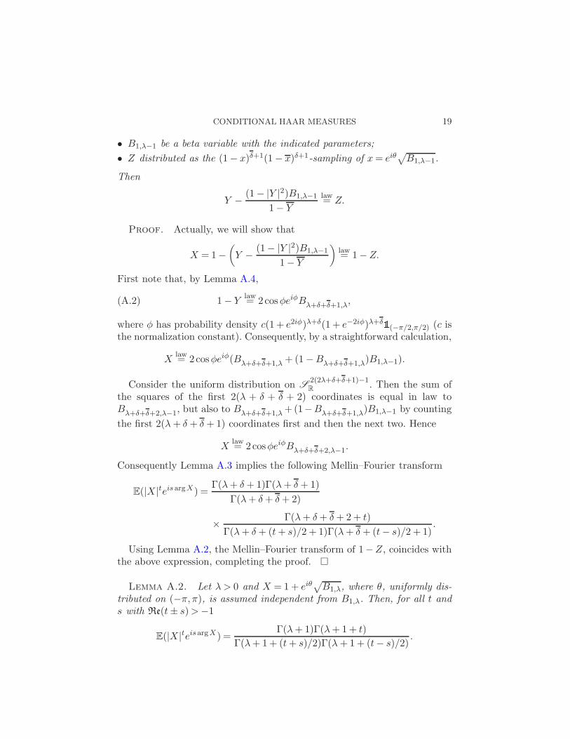
• B1,λ−1 be a beta variable with the indicated parameters;

• Z distributed as the (1− x)δ+1(1− x)δ+1-sampling of x = eiθ√

B1,λ−1.

Then

Y − (1− |Y |2)B1,λ−1

1− Y

law= Z.

Proof. Actually, we will show that

X = 1−(

Y − (1− |Y |2)B1,λ−1

1− Y

)

law= 1−Z.

First note that, by Lemma A.4,

1− Ylaw= 2cosφeiφBλ+δ+δ+1,λ,(A.2)

where φ has probability density c(1 + e2iφ)λ+δ(1 + e−2iφ)λ+δ1(−π/2,π/2) (c isthe normalization constant). Consequently, by a straightforward calculation,

Xlaw= 2cosφeiφ(Bλ+δ+δ+1,λ + (1−Bλ+δ+δ+1,λ)B1,λ−1).

Consider the uniform distribution on S2(2λ+δ+δ+1)−1R

. Then the sum ofthe squares of the first 2(λ + δ + δ + 2) coordinates is equal in law toBλ+δ+δ+2,λ−1, but also to Bλ+δ+δ+1,λ +(1−Bλ+δ+δ+1,λ)B1,λ−1 by counting

the first 2(λ + δ + δ + 1) coordinates first and then the next two. Hence

Xlaw= 2cosφeiφBλ+δ+δ+2,λ−1.

Consequently Lemma A.3 implies the following Mellin–Fourier transform

E(|X|teisargX) =Γ(λ + δ + 1)Γ(λ + δ + 1)

Γ(λ + δ + δ + 2)

× Γ(λ + δ + δ + 2 + t)

Γ(λ + δ + (t + s)/2 + 1)Γ(λ + δ + (t− s)/2 + 1).

Using Lemma A.2, the Mellin–Fourier transform of 1−Z, coincides withthe above expression, completing the proof. �

Lemma A.2. Let λ > 0 and X = 1 + eiθ√

B1,λ, where θ, uniformly dis-tributed on (−π,π), is assumed independent from B1,λ. Then, for all t ands with Re(t± s) > −1

E(|X|teisargX) =Γ(λ + 1)Γ(λ + 1 + t)

Γ(λ + 1 + (t + s)/2)Γ(λ + 1 + (t− s)/2).

20 P. BOURGADE

Proof. First, note that

E(|X|teisargX) = E((1 + eiθ√

B1,λ)a(1 + e−iθ√

B1,λ)b)

with a = (t + s)/2 and b = (t− s)/2. Recall that if |x|< 1 and u ∈ R then

(1 + x)u =∞∑

k=0

(−1)k(−u)kk!

xk,

where (y)k = y(y+1) · · · (y+k−1) is the Pochhammer symbol. As |eiθ√

B1,λ|<1 a.s., we get

E[|X|teisargX ] = E

[( ∞∑

k=0

(−1)k(−a)kk!

Bk/21,λ eikθ

)( ∞∑

ℓ=0

(−1)ℓ(−b)ℓℓ!

Bℓ/21,λe−iℓθ

)]

.

After expanding this double sum [it is absolutely convergent because Re(t±s) > −1], all terms with k 6= ℓ will give an expectation equal to 0, so as

E(Bk1,λ) = Γ(1+k)Γ(λ+1)

Γ(1)Γ(λ+1+k) = k!(λ+1)k

,

E[|X|teisargX ] =∞∑

k=0

(−a)k(−b)kk!(λ + 1)k

.

Note that this series is equal to the value at z = 1 of the hypergeometricfunction 2F1(−a,−b,λ + 1; z). This value is well known (see, e.g., [1]) andyields:

E[|X|teisargX ] =Γ(λ + 1)Γ(λ + 1 + a + b)

Γ(λ + 1 + a)Γ(λ + 1 + b).

This is the desired result. �

Lemma A.3. Take φ with probability density c(1 + e2iφ)z(1 + e−2iφ)z ×1(−π/2,π/2), where c is the normalization constant, Re(z) > −1/2. Let X =

2cosφeiφ. Then

E[|X|teisargX ] =Γ(z + 1)Γ(z + 1)

Γ(z + z + 1)(A.3)

× Γ(z + z + t + 1)

Γ(z + (t + s)/2 + 1)Γ(z + (t− s)/2 + 1).

Proof. From the definition of X ,

E(|X|teisargX) = c

∫ π/2

−π/2(1 + e2ix)z+(t+s)/2(1 + e−2ix)z+(t−s)/2 dx.

CONDITIONAL HAAR MEASURES 21

Both terms on the RHS can be expanded as a series in e2ix or e−2ix for allx 6= 0. Integrating over x between −π/2 and π/2, only the diagonal termsremain, and so

E(|X|teisargX) = c∞∑

k=0

(−z − (+t + s)/2)k(−z − (t− s)/2)k(k!)2

.

The value of a 2F1 hypergeometric functions at z = 1 is well known (see,e.g., [1]), hence

E(|X|teisargX) = cΓ(z + z + t + 1)

Γ(z + (t + s)/2 + 1)Γ(z + (t− s)/2 + 1).

As this is 1 when s = t = 0, c = Γ(z+1)Γ(z+1)Γ(z+z+1) , which completes the proof. �

Lemma A.4. Let λ > 2, Re(δ) > −1/2, θ uniform on (−π,π) and B1,λ−1

a beta variable with the indicated parameters. Let Y be distributed as the

(1− x)δ(1− x)δ-sampling of x = eiθ√

B1,λ−1. Then

1− Ylaw= 2cosφeiφBλ+δ+δ,λ−1

with Bλ+δ+δ,λ−1 a beta variable with the indicated parameters and, indepen-

dently, φ having probability density c(1+e2iφ)λ+δ−1(1+e−2iφ)λ+δ−11(−π/2,π/2)

(c is the normalization constant).

Proof. The Mellin–Fourier transform of X = 1 − Y can be evaluatedusing Lemma A.2, and equals

E(|X|teisargX) =Γ(λ + δ)Γ(λ + δ)Γ(λ + t + δ + δ)

Γ(λ + (t + s)/2 + δ)Γ(λ + (t− s)/2 + δ)Γ(λ + δ + δ).

On the other hand, using Lemma A.3 and (A.1), the Mellin–Fourier trans-form of 2 cosφeiφBn+δ+δ,λ coincides with the above result. �

REFERENCES

[1] Andrews, G. E., Askey, R. and Roy, R. (1999). Special Functions. Encyclopediaof Mathematics and Its Applications 71. Cambridge Univ. Press, Cambridge.MR1688958

[2] Borodin, A. and Olshanski, G. (2001). Infinite random matrices and ergodic mea-sures. Comm. Math. Phys. 223 87–123. MR1860761

[3] Bourgade, P., Hughes, C. P., Nikeghbali, A. and Yor, M. (2008). The charac-teristic polynomial of a random unitary matrix: A probabilistic approach. DukeMath. J. 145 45–69. MR2451289

[4] Bourgade, P., Nikeghbali, A. and Rouault, A. (2008). Hua–Pickrell measureson general compact groups. Preprint.

22 P. BOURGADE

[5] Bourgade, P., Nikeghbali, A. and Rouault, A. (2008). Circular Jacobi ensemblesand deformed Verblunsky coefficients. Preprint.

[6] Bump, D. (2004). Lie Groups. Graduate Texts in Mathematics 225. Springer, NewYork. MR2062813

[7] Costin, O. and Lebowitz, J. (1995). Gaussian fluctuations in random matricesPhys. Rev. Lett. 75 69–72.

[8] Keating, J. P. and Snaith, N. C. (2000). Random matrix theory and ζ(1/2 + it).Comm. Math. Phys. 214 57–89. MR1794265

[9] Killip, R. and Nenciu, I. (2004). Matrix models for circular ensembles. Int. Math.Res. Not. 50 2665–2701. MR2127367

[10] Miller, S. J. (2006). Investigations of zeros near the central point of elliptic curveL-functions. Experiment. Math. 15 257–279. MR2264466

[11] Petrov, V. V. (1995). Limit Theorems of Probability Theory: Sequences of Inde-pendent Random Variables. Oxford Studies in Probability 4. Oxford Univ. Press,New York. MR1353441

[12] Selberg, A. (1992). Old and new conjectures and results about a class of Dirich-let series. In Proceedings of the Amalfi Conference on Analytic Number Theory(Maiori, 1989) 367–385. Univ. Salerno, Salerno. MR1220477

[13] Snaith, N. C. (2005). Derivatives of random matrix characteristic polynomials withapplications to elliptic curves. J. Phys. A 38 10345–10360. MR2185940

[14] Snaith, N. C. (2007). The derivative of SO(2N + 1) characteristic polynomials andrank 3 elliptic curves. In Ranks of Elliptic Curves and Random Matrix Theory.London Mathematical Society Lecture Note Series 341 93–107. Cambridge Univ.Press, Cambridge. MR2322339

[15] Yor, M. (2008). A further note on Selberg’s integrals, inspired by N. Snaith’s resultsabout the distribution of some characteristic polynomials, RIMS Kokyuroku.

Telecom Paris Tech

46 rue Barrault

75634 Paris Cedex 13

France

E-mail: bourgade@enst.fr