
Condition Numbers in the Boundary Element Method: …hochsten/pdf/dijkstra-thesis.pdf · Condition...
181
Condition Numbers in the Boundary Element Method: Shape and Solvability
-
Upload
truonglien -
Category
Documents
-
view
220 -
download
0
Transcript of Condition Numbers in the Boundary Element Method: …hochsten/pdf/dijkstra-thesis.pdf · Condition...

Condition Numbers in the BoundaryElement Method:
Shape and Solvability

Copyright c©2008 by W. Dijkstra, Eindhoven, The Netherlands.All rights are reserved. No part of this publication may be reproduced, stored in aretrieval system, or transmitted, in any form or by any means, electronic, mechanical,photocopying, recording or otherwise, without prior permission of the author.Printed by Eindhoven University PressCover design: Creanza media
cover background: Victor Vasarely
CIP-DATA LIBRARY TECHNISCHE UNIVERSITEIT EINDHOVEN
Dijkstra, Willem
Condition numbers in the boundary element method : shape andsolvability /door Willem Dijkstra. -Eindhoven: Technische Universiteit Eindhoven, 2008.
Proefschrift. -ISBN 978-90-386-1245-4
NUR 919Subject headings: boundary element methods / integral equations ; numericalmethods / numerical simulation / Navier-Stokes equations /glass2000 Mathematics Subject Classification:65N38, 74S15, 65R20, 35Q30, 76D05

Condition Numbers in the BoundaryElement Method:
Shape and Solvability
PROEFSCHRIFT
ter verkrijging van de graad van doctor aan deTechnische Universiteit Eindhoven, op gezag van de
Rector Magnificus, prof.dr.ir. C.J. van Duijn, voor eencommissie aangewezen door het College voor
Promoties in het openbaar te verdedigenop donderdag 17 april 2008 om 16.00 uur
door
Willem Dijkstra
geboren te Driebruggen

Dit proefschrift is goedgekeurd door de promotor:
Prof.dr. R.M.M. Mattheij
Copromotor:Dr. M.E. Hochstenbach

Apply your heart to instruction,and your ears to words of knowledge
Proverbs 23:12 (NKJ)

Contents
1 Introduction 11.1 Problem setting . . . . . . . . . . . . . . . . . . . . . . . . . . . . 11.2 Boundary Element Method . . . . . . . . . . . . . . . . . . . . . . 21.3 Condition number . . . . . . . . . . . . . . . . . . . . . . . . . . . 41.4 Condition numbers of the BEM-matrices . . . . . . . . . . . . . . . 51.5 Objectives . . . . . . . . . . . . . . . . . . . . . . . . . . . . . . . 61.6 Outline of the thesis . . . . . . . . . . . . . . . . . . . . . . . . . . 8
2 Boundary Element Method 102.1 Integral Equations . . . . . . . . . . . . . . . . . . . . . . . . . . . 102.2 Operator theory . . . . . . . . . . . . . . . . . . . . . . . . . . . . 152.3 Algebraic Equations . . . . . . . . . . . . . . . . . . . . . . . . . . 172.4 Matrix Elements . . . . . . . . . . . . . . . . . . . . . . . . . . . . 202.5 Numerical integration . . . . . . . . . . . . . . . . . . . . . . . . . 22
3 Laplace equation at two-dimensional domain 243.1 Eigenvalues ofKs andKd . . . . . . . . . . . . . . . . . . . . . . 243.2 Eigenvalues of the matrices . . . . . . . . . . . . . . . . . . . . . . 273.3 Dirichlet problem . . . . . . . . . . . . . . . . . . . . . . . . . . . 293.4 Neumann problem . . . . . . . . . . . . . . . . . . . . . . . . . . 323.5 Mixed boundary conditions . . . . . . . . . . . . . . . . . . . . . . 343.6 Decoupled equations . . . . . . . . . . . . . . . . . . . . . . . . . 43
4 Logarithmic capacity 474.1 Introduction . . . . . . . . . . . . . . . . . . . . . . . . . . . . . . 474.2 Logarithmic capacity . . . . . . . . . . . . . . . . . . . . . . . . . 504.3 Dirichlet problem . . . . . . . . . . . . . . . . . . . . . . . . . . . 514.4 Mixed problem . . . . . . . . . . . . . . . . . . . . . . . . . . . . 534.5 Neumann problem . . . . . . . . . . . . . . . . . . . . . . . . . . 554.6 Examples . . . . . . . . . . . . . . . . . . . . . . . . . . . . . . . 57
vi

CONTENTS vii
5 Two-dimensional Stokes flow 655.1 Boundary integral equations for 2D Stokes flow . . . . . . . . .. . 655.2 Eigensystem of the single layer operatorG at a circle . . . . . . . . 675.3 Invertibility of single layer operator on general domain . . . . . . . 705.4 Invertibility of operator on general domain with mixed conditions . 735.5 Numerical examples . . . . . . . . . . . . . . . . . . . . . . . . . 765.6 Blowing problem in 2D . . . . . . . . . . . . . . . . . . . . . . . . 86
6 Three-dimensional Stokes flow 946.1 Simulating the blowing of glass containers with the BEM .. . . . . 946.2 Mathematical model . . . . . . . . . . . . . . . . . . . . . . . . . 966.3 Boundary integral equations . . . . . . . . . . . . . . . . . . . . . 1036.4 Numerical solution . . . . . . . . . . . . . . . . . . . . . . . . . . 1066.5 Time integration and post-processing . . . . . . . . . . . . . . .. . 108
7 Results 1117.1 Glass blowing . . . . . . . . . . . . . . . . . . . . . . . . . . . . . 1117.2 Curvature driven flow . . . . . . . . . . . . . . . . . . . . . . . . . 1237.3 Parameter analysis . . . . . . . . . . . . . . . . . . . . . . . . . . 128
A Curvature approximation 134
B Contact problem 142
C Smoothing techniques 149C.1 Laplacian smoothing . . . . . . . . . . . . . . . . . . . . . . . . . 149C.2 Smoothing scalar function . . . . . . . . . . . . . . . . . . . . . . 151C.3 Smoothing vector field . . . . . . . . . . . . . . . . . . . . . . . . 152
Bibliography 155
Index 162
Summary 166
Samenvatting 169
Acknowledgements 172
Curriculum vitae 173

viii CONTENTS

Chapter 1
Introduction
In mathematics you don’t understandthings. You just get used to them.
J. von Neumann [99]
1.1 Problem setting
Today many commercially available mathematical software tools exist that solve alarge variety of mathematical problems. Often these tools are being used in a “blackbox” approach. The user inserts a mathematical problem and obtains a solution forit, without too much knowledge of what is happening behind the scene. Of course,software manufacturers claim that there is no need to have detailed information on theworking of their products. Regardless of the mathematical problem that is inserted,the software will produce the correct solution. The question is whether this is alwaystrue.
Typically, in software tools a mathematical problem is defined on an object thathas a certain size and shape. The user assumes that the success of solving the problemdoes not depend on this size and shape. For instance, if a correct solution is obtainedfor a square object, we expect a correct solution for the samemathematical problemfor a rectangular object. If a correct solution is obtained for a circular object, weexpect a correct solution for a circular object that is twiceas large.
The mathematical software tools employ several numerical methods that solvemathematical problems. One such method is the boundary element method (BEM),which is the topic of this thesis. The success of this particular method to solve certainmathematical problems may depend on the size and shape of theobjects on whichthe problems are defined. If the BEM is able to solve a problem on a certain object,it is not necessarily able to solve the problem on an object that is slightly larger or
1

2 Chapter 1 Introduction
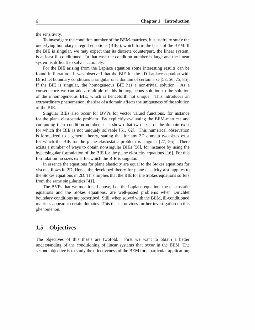
Figure 1.1: In most numerical methods both the interior and the boundaryof a domainneed to be discretised (left). In the boundary element method only the boundary needs to bediscretised (right).
smaller. This has its effect on the software that is built upon the BEM. The userof such software must be aware that solutions provided by thesoftware may not becorrect. Hence in these cases detailed information on the working of the software,i.e. on the numerical method, is essential in judging the correctness of solutions. Thisthesis addresses the working of the BEM and investigates under which conditions itproduces correct solutions.
1.2 Boundary Element Method
The BEM is a numerical method that approximates solutions ofboundary valueproblems (BVPs). The method is a relatively young method as its birth can be placedin the sixties. Compared to the finite element method (FEM), the development of theBEM has been substantially slower. One reason for this slower development in theBEM is the limited availability of fundamental solutions ofthe BVPs. Another reasonis likely to be the involvement of singular integral equations that need to be solved.Today these equations are well-understood, and the number of application fields inwhich the BEM is used is large, although not as large as for thefinite element method.
The most important aspect in which the BEM distinguishes itself from othernumerical methods is the fact that only the boundary of a domain needs to bediscretised. In many other numerical methods, such as the FEM, finite differences orthe finite volume method, in addition to the boundary, the interior of the domain alsoneeds to be discretised (Figure 1.1). As a consequence of theboundary discretisation,the BEM is a suitable method for problems on external domains, or domains that havea free or moving boundary. Also problems in which singularities or discontinuitiesoccur can be handled efficiently by the BEM. Another advantage of the BEM is thatvariables and their derivatives, for instance temperatureand its flux, are computedwith the same degree of accuracy.

Section 1.2 Boundary Element Method 3
Integral equations constitute the foundation of the BEM, and have been knownfor more than a century. In particular, it is known for a long time that the solutionsof BVPs can also be expressed as solutions of an integral equation. As early as 1903Fredholm already used discretised integral equations for potential problems [43].His work can be considered the basis for the indirect formulation of the BEM; thefunctions that appear in theindirect formulation do not have a physical meaning,though physical quantities can be derived from these functions. The basis of thedirect formulation can be placed at Somigliana [86] in 1886, who presented anintegral equation relating displacements and stresses. A large number of books andpapers have appeared on the subject of integral equations inpotential and elasticitytheory by mathematicians, such as Kellogg [58], Muskhelishvili [74], Mikhlin [73]and Kupradze [63]. Their results are, however, limited to simple problems as theintegral equations have to be solved with analytical procedures and without the aidof computers.
The breakthrough in the development of the BEM came in the nineteen sixties.Jaswon [55] and Symm [90] discretised the integral equations for two-dimensionalpotential problems by approximating the boundary of a domain by a set of straightlines. At each line element the functions are approximated by constants. Theirmethod has a semi-direct formulation, as the functions needto be differentiated orintegrated to obtain physical quantities. A direct formulation has been introduced byRizzo [80], who also used discretised integral equations torelate displacements andtractions in two-dimensional elasticity theory. The extension to three dimensions hasbeen given by Cruse [31], using triangular elements to describe the domain boundary.
In the late sixties and early seventies the number of applications for whichboundary elements are used grew. This constituted a firm foundation for the furtherdevelopment of the BEM and proved that the BEM is a powerful and accuratetechnique. At this stage attention was also paid to the errorand convergence analysisof the BEM. An important contribution came from Hsiao and Wendland [54], whoperformed such error and convergence analysis for theGalerkin formulation ofboundary integral equations. As opposed to the Galerkin formulation, thepointcollocationformulation yields easier approximations of integral equations. The erroranalysis for this type of boundary elements was performed byArnold, Saranen andWendland [3, 4, 83] during the eighties.
The first book covering the numerical solution of boundary integral equationshas been published by Jaswon and Symm [56] in 1977. Not much later Brebbia [9]used the terminology “Boundary Elements” for the first time as opposed to “FiniteElements”. As of now, the BEM proves to be an effective alternative to solvemany engineering problems from a variety of application fields, for instanceacoustics, fracture mechanics, potential theory, elasticity theory, viscous flows,thermodynamics, etc.

4 Chapter 1 Introduction
1.3 Condition number
One way to measure the ability of a numerical method to accurately solvemathematical problems is by monitoring the so-calledcondition number. In thisthesis we compute or estimate the condition numbers that appear in the BEM to seewhether this method is able to solve mathematical problems accurately.
To explain the meaning of the condition number we first need toaddress the termswell-conditionedandill-conditioned. In general a problem is called well-conditionedif a small change in the input data does not result in a large change in the problem’ssolution. A problem is called ill-conditioned if a small change in the input datacauses a large change in the solution. Depending on how one defines “large” and“small”, this classification enables us to divide problems into well-conditioned andill-conditioned problems. However it does not provide any information on the degreeof ill-conditioning. The condition number does precisely that.
Within the setting of this thesis, the condition number ranges from one to infinity.If the condition number is equal to one, then a problem is verywell-conditioned.If a problem is singular, the condition number is infinitely large. For problems thatapproach a singular problem, the condition number approaches infinity. Hence suchproblems are very ill-conditioned.
In this thesis we study the condition number of linear systems of algebraicequations, which are problems of the form
Ax = b. (1.1)
Such systems are the result of discretising the integral equations that appear in theBEM. The success of solving the linear system depends to a large extent on thecondition number of the system matrixA. If the condition number of this matrixis very large, then the linear system is difficult to solve accurately. Moreover, if thecondition number is large, the solutionx is sensitive to perturbations in the inputdatab.
It is unclear when the concept of condition number, and related to that the termill-conditioned, was introduced. In 1948 Turing [92] mentioned that
... the expression ‘ill-conditioned’ is sometimes used merely as aterm of abuse applicable to matrices or equations, but it seems often tocarry a meaning somewhat similar to that defined below.
Evidently the term ill-conditioned was already in use at that time. In his paper Turingintroduced the normN(A) and the maximum coefficientM(A) of a matrixA by
N(A) :=(∑
i,j
a2ij
)1/2,
M(A) := maxi,j
|aij |, (1.2)

Section 1.4 Condition numbers of the BEM-matrices 5
in which we recognizeN(A) as the Frobenius norm andM(A) as the maximumnorm where the matrixA is seen as a vector of numbers. With these two quantitiesTuring defined theN-condition numberas 1
nN(A)N(A−1) and theM-conditionnumberasnM(A)M(A−1), wheren is the size of the matrix. He claimed thatthese condition numbers are a measure of the degree of ill-conditioning in a matrix.Ironically, the quantity that is now known as the spectral norm of a matrix was alsodefined by Turing under the namemaximum expansion. He did not use this quantityto define a related condition number however. Therefore the number that is nowadaysreferred to as the condition number does not exactly match the condition numbersdefined by Turing.
1.4 Condition numbers of the BEM-matrices
Today the BEM is widely used in many application fields. Regrettably the issue ofconditioning is often neglected. Usually when solving a BVPwith the BEM, it isassumed that the condition number of the resulting system matrix is modest. Thequestion is whether this is true.
First we need to remark that a BVP that is ill-posed will automatically lead toBEM-matrices that have large condition numbers. These BVPsare therefore notthe most interesting problems to investigate. A more interesting question is whetherwell-posed BVPs can lead to BEM-matrices that have large condition numbers. It isthis last class of BVPs that we focus on in this thesis.
Until now little little attention has been given to the condition number of BEM-matrices. It has been proven that the condition number of thesystem matrix is atleast orderN , whereN is the number of boundary elements on a two-dimensionaldomain [97]. This holds for the BEM-matrices that correspond to potential problemswith Dirichlet boundary conditions. Similar results are derived by others [21],who have shown that some small modifications to the algebraicset of equationscan improve the conditioning of the linear system. In a detailed study for twospecific domains, namely the circle and the ellipse, the BEM is applied to theLaplace equation with Dirichlet boundary conditions [19, 20]. For both domainsanalytical expressions for the condition number of the BEM-matrix are derived.These expressions show the dependance of the condition number on the radius ofthe circle or the aspect ratio of the ellipse. The Laplace equation on a circle withDirichlet boundary conditions has been the topic of severalother papers [22, 24];special attention is given to the so-calledlocal condition number. It is claimed thatthis local condition number is a more accurate indicator forthe sensitivity of a linearsystem than the ordinary condition number, which gives too pessimistic estimates of
6 Chapter 1 Introduction
the sensitivity.To investigate the condition number of the BEM-matrices, itis useful to study the
underlying boundary integral equations (BIEs), which formthe basis of the BEM. Ifthe BIE is singular, we may expect that its discrete counterpart, the linear system,is at least ill-conditioned. In that case the condition number is large and the linearsystem is difficult to solve accurately.
For the BIE arising from the Laplace equation some interesting results can befound in literature. It was observed that the BIE for the 2D Laplace equation withDirichlet boundary conditions is singular on a domain of certain size [53, 56, 75, 85].If the BIE is singular, the homogeneous BIE has a non-trivialsolution. As aconsequence we can add a multiple of this homogeneous solution to the solutionof the inhomogeneous BIE, which is henceforth not unique. This introduces anextraordinary phenomenon; the size of a domain affects the uniqueness of the solutionof the BIE.
Singular BIEs also occur for BVPs for vector valued functions, for instancefor the plane elastostatic problem. By explicitly evaluating the BEM-matrices andcomputing their condition numbers it is shown that two sizesof the domain existfor which the BIE is not uniquely solvable [51, 62]. This numerical observationis formalized to a general theory, stating that for any 2D domain two sizes existfor which the BIE for the plane elastostatic problem is singular [27, 95]. Thereexists a number of ways to obtain nonsingular BIEs [50], for instance by using thehypersingular formulation of the BIE for the plane elasticity equations [16]. For thisformulation no sizes exist for which the BIE is singular.
In essence the equations for plane elasticity are equal to the Stokes equations forviscous flows in 2D. Hence the developed theory for plane elasticity also applies tothe Stokes equations in 2D. This implies that the BIE for the Stokes equations suffersfrom the same singularities [41].
The BVPs that we mentioned above, i.e. the Laplace equation,the elastostaticequations and the Stokes equations, are well-posed problems when Dirichletboundary conditions are prescribed. Still, when solved with the BEM, ill-conditionedmatrices appear at certain domains. This thesis provides further investigation on thisphenomenon.
1.5 Objectives
The objectives of this thesis are twofold. First we want to obtain a betterunderstanding of the conditioning of linear systems that occur in the BEM. Thesecond objective is to study the effectiveness of the BEM fora particular application;

Section 1.5 Objectives 7
the simulation of the blowing phase in the industrial production process of glassbottles and jars.
1.5.1 Solvability
Almost all research that has been performed on condition numbers and boundaryintegral equations concerns BVPs with Dirichlet boundary conditions. For BVPswith mixed boundary conditions hardly any results are present. BVPs with mixedboundary conditions is therefore one of the topics of this thesis. We investigate thecondition numbers of the matrices that appear when the BEM isused to solve suchBVPs.
For the BEM-matrix arising from the Laplace equation with mixed boundaryconditions on a circle it is possible to estimate its condition number. We show thatthis matrix is well-conditioned, except for the unit circleand circles that are close tothe unit circle. In these cases the condition number is (infinitely) large.
For the BEM-matrix for the Laplace equation with mixed boundary conditionson an arbitrary 2D domain it can be shown that there is one specific scaling of thatdomain for which the condition number is infinitely large. The scaling for whichthis happens is called thecritical scaling and the corresponding domain thecriticaldomain.
The BEM-matrix for the Stokes equations with mixed boundaryconditions onan arbitrary domain can also have an infinitely large condition number for certaindomains. As the corresponding BIE consists of two equations, there exist twoscalings of the domain at which the condition number becomesinfinitely large.
There are several ways to avoid the infinitely large condition numbers at criticaldomains. The simplest remedy is to rescale the domain to another size such that thecondition number is bounded. Another option is to add an extra equation to the linearsystem that guarantees low condition numbers. This extra equation is a compatibilitycondition that stems from the BVP. A drawback of this option is that we have to solvea system with a rectangular matrix, which requires different solution techniques. Athird option is to slightly modify the fundamental solutionof the BVP. By includinga scaling parameter in this fundamental solution it can be shown that the conditionnumbers of the BEM-matrices remain bounded at the critical domains.
1.5.2 Blowing of glass
The singular BIEs that we mentioned above typically occur ina 2D setting. This isa direct consequence of the logarithmic nature of the fundamental solution for BVPsthat contain the Laplace operator. Hence prudence is calledfor when one applies theBEM to BVPs on a 2D domain. In a 3D setting the fundamental solution for BVPswith the Laplace operator does not have a logarithmic term. Therefore singular BIEs

8 Chapter 1 Introduction
similar to those in 2D do no occur in 3D. This allows us to safely apply the BEM toBVPs in 3D that contain the Laplace operator.
As a special application we consider the blowing problem of viscous fluids. Inthis problem a viscous fluid is positioned in a mould and blownto a desired shape.This blowing process takes place, amongst others, in the industrial manufacturing ofglass bottles and jars. The flow of the fluid is governed by the Stokes equations andcan be solved with the BEM. This problem typically involves afree boundary. Wewill investigate whether the BEM is an appropriate numerical method to solve such aproblem.
We are aware of several formulations of the BEM. In this thesis we choosefor the direct symmetric collocation formulation. The direct formulation involvesfunctions that have a physical meaning, whereas the indirect formulation usesauxiliary functions that have no physical meaning. The symmetric formulation,involving the single and double layer operators, is more commonly used than the non-symmetric formulation, which incorporates the hypersingular operator. We preferthe collocation method above the Galerkin method. Again thecollocation methodis more commonly used and it does not require a second integration step like theGalerkin method does.
1.6 Outline of the thesis
The thesis starts with an introduction on the BEM inChapter 2. We demonstrate howa BVP can be translated into a BIE, and after discretisation of the domain boundary,into a system of linear equations. We illustrate this for thecase of the Laplaceequation, but the techniques used to derive the linear system are similar for otherBVPs. We also present a number of fundamental results on the boundary integraloperators that appear in the BIE.
In the Chapters 3 and4 we study the BEM-matrices for the Laplace equationon two-dimensional domains.Chapter 3 concentrates on the Laplace equationon a circular domain with mixed boundary conditions. The eigenvalues of thecorresponding BEM-matrix are approximated, which resultsin an estimate for thecondition number of the BEM-matrix.Chapter 4 generalizes the results to Laplaceequations on arbitrary 2D domains. For this general class ofproblems it is notpossible to estimate the condition number of the BEM-matrixaccurately, though it isproven that for certain domains the condition number is infinitely large. This holdsfor both Laplace equations with Dirichlet conditions and mixed conditions. Thisphenomenon is confirmed by a number of numerical examples on circles, ellipses,squares and triangles. The large condition numbers can be avoided by making small
Section 1.6 Outline of the thesis 9
modifications to the standard boundary element formulation. We present a numberof remedies that guarantee low condition numbers.
The extension to BVPs for vector-valued functions is described inChapter 5.Here we focus on the Stokes equations on a 2D domain. Again it is shown that forcertain domains the condition number of the corresponding BEM-matrix becomesinfinitely large. This happens both for the Stokes equationswith Dirichlet conditionsand mixed conditions. We present a number of numerical examples that illustrate thisphenomenon. To avoid condition numbers that are infinitely large at certain domainswe list several remedies that are more or less similar to the remedies for the Laplaciancase.
The domains for which the condition numbers become infinitely large only occurin 2D. Therefore we can safely apply the BEM on a 3D problem. IntheChapters 6and7 we simulate the blowing phase of glass containers. InChapter 6 we presentthe mathematical model that describes this blowing problem. The starting point arethe Navier-Stokes equations that describe the flow of a fluid in 3D. These equationscan be reduced to the Stokes equations as the fluid is a creeping viscous flow. It isshown how to transform the Stokes equations to a set of BIEs. After discretisationof the domain we obtain a system of linear equations. In this way we can computethe velocity of the glass at any point in time. We use a time integration method totrack the position of the glass surface as time evolves.Chapter 7 gives numericalresults for the blowing problem. We simulate the blowing of several containers for anumber of different moulds. We also show another application that can be simulatedwith the help of the mathematical model for the blowing problem; the evolution ofviscous drops. Such drops, regardless of their initial size, deform to a spherical drop.We illustrate this process for drops that have the initial shape of an ellipsoide and abeam. We conclude this chapter by investigating the role of the various forces thatappear in the blowing problem, such as gravity, surface tension and frictional forces.

Chapter 2
Boundary Element Method
This chapter introduces the basics of the boundary element method (BEM). Themethod aims at approximating solutions of boundary value problems (BVPs). Inparticular we use the Laplace equation on a 2D domain as an example to presentthe BEM formulation. For other BVPs the BEM formulation can be obtained in asimilar manner. First we transform the BVP into a boundary integral equation usingGreen’s second identity. Then we discretise the boundary ofthe domain and obtaina linear system of algebraic equations. Finally we pay attention to the calculation ofthe matrices that appear in these algebraic equations. The BEM that we present hereis the collocation method in a direct formulation, which means that the variables inthe method represent physical quantities.
2.1 Integral Equations
We consider a simply connected domainΩ in R2 with boundaryΓ = ∂Ω. Denote by
n the outward normal onΓ. The functionu(x) = u(x, y) for x ∈ Ω is the solutionof the Laplace equation, i.e.
∇2u :=∂2u
∂x2+∂2u
∂y2= 0, x ∈ Ω. (2.1)
As we will study mixed boundary conditions in this thesis, wedivide the boundaryΓinto two parts,Γ = Γu ∪ Γq. At Γu we pose Dirichlet boundary conditions and atΓq
we pose Neumann conditions. We introduce the notationq := ∂u/∂n as the normalderivative ofu onΓ. Then the BVP foru with mixed boundary conditions reads
∇2u = 0, x ∈ Ω,u = u, x ∈ Γu,q = q, x ∈ Γq,
(2.2)
10

Section 2.1 Integral Equations 11
W
G q
n
G u
Figure 2.1: The domainΩ with boundaryΓ, which is divided into a Dirichlet partΓu and aNeumann partΓq.
whereu andq are known functions representing the boundary data.Let xP andxQ be two points inΩ. The Euclidean distance betweenxP andxQ
is
r(xP ,xQ) := ‖xP − xQ‖2 =√
(xP − xQ)2 + (yP − yQ)2. (2.3)
A fundamental solution for the Laplace operator∇2 is given by
G(xP ,xQ) :=1
2πlog
1
r(xP ,xQ), xP ,xQ ∈ Ω, (2.4)
which means that
∇2QG(xP ,xQ) = −δ(xP − xQ), xP ,xQ ∈ Ω. (2.5)
The subscriptQ of the Laplace operator denotes differentiation toxQ andδ(x) is theDirac-delta function. Note thatGα(xP ,xQ) := 1/2π log(α/r(xP ,xQ)), α ∈ R
+,is also a fundamental solution for the Laplace operator. Theparameterα can bechosen as a characteristic length scale of the domainΩ, thus making the argument ofthe logarithm dimensionless.
Green’s second identity for two functionsu andv states that∫
Ω
(
u(xQ)∇2v(xQ) − v(xQ)∇2u(xQ))
dΩ =
∫
Γ
(
u(xQ)∂v
∂n(xQ) − v(xQ)
∂u
∂n(xQ)
)
dΓ. (2.6)

12 Chapter 2 Boundary Element Method
x p
B e
e
WG
n
G en
q
Figure 2.2: The pointxP lies in the interior of the domain.
For u we substitute the solution of the BVP (2.2), and forv we substitute thefundamental solutionG(xP ,xQ), where xP is regarded as a parameter. As∇2u(xQ) = 0 in Ω, Green’s second identity yields
∫
Ω
u(xQ)∇2QG(xP ,xQ)dΩQ =
∫
Γ
(
u(xQ)∂G
∂nQ(xP ,xQ) −G(xP ,xQ)q(xQ)
)
dΓQ. (2.7)
The integrals that appear in this identity must be evaluatedcarefully, as thefundamental solutionG has a logarithmic singularity atxQ = xP . Hence thelocation ofxP greatly influences the outcome of the integrals.
First we consider the case thatxP is in the interior of the domainΩ. In that casewe position a small circleBε with radiusε and boundaryΓε around the pointxP ,such that the entire circle is in the interior ofΩ, as is shown in Figure 2.2. In this wayG does not have a singularity in the domainΩ − Bε and we have∇2
QG = 0 in thisnew domain. Green’s second identity applied to the domainΩ −Bε becomes
∫
Γ+Γε
(
u(xQ)∂G
∂nQ(xP ,xQ) −G(xP ,xQ)q(xQ)
)
dΓQ = 0, xP ∈ Ω, (2.8)
Note that no domain integrals appear in this identity. The remaining boundaryintegral consists of two contributions; an integral overΓ and an integral over thecircular boundaryΓε. The outward normal onΓε is in the direction of the pointxP .Therefore the local coordinateθ that describesΓε, runs in clockwise direction over
Section 2.1 Integral Equations 13
the boundary,0 ≤ θ < 2π. To calculate the integral overΓε we note that∂G
∂nQ(xP ,xQ)
∣∣∣xQ∈Γε
= −∂G∂r
(xP ,xQ)∣∣∣xQ∈Γε
=1
2πr
∣∣∣xQ∈Γε
=1
2πε. (2.9)
Hence the integral overΓε amounts to∫
Γε
(
u(xQ)∂G
∂nQ(xP ,xQ) −G(xP ,xQ)q(xQ)
)
dΓQ
=1
2π
2π∫
0
(
u(xQ)1
ε− log
1
εq(xQ)
)
εdθ
=1
2π
2π∫
0
(
u(xQ) + ε log ε q(xQ))
dθ. (2.10)
As ε log ε → 0 for ε ↓ 0, the last integral approachesu(xP ) whenε tends to zero.Substituting this in (2.8) we obtain
u(xP ) +
∫
Γ
(
u(xQ)∂G
∂nQ(xP ,xQ) −G(xP ,xQ)q(xQ)
)
dΓQ = 0, (2.11)
for xP ∈ Ω. This identity relates the values ofu in internal pointsxP to values ofuandq at the boundary.
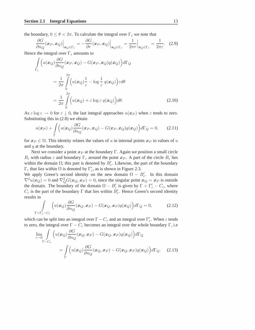
Next we consider a pointxP at the boundaryΓ. Again we position a small circleBε with radiusε and boundaryΓε around the pointxP . A part of the circleBε lieswithin the domainΩ; this part is denoted byB′
ε. Likewise, the part of the boundaryΓε that lies withinΩ is denoted byΓ′
ε, as is shown in Figure 2.3.We apply Green’s second identity on the new domainΩ − B′
ε. In this domain∇2u(xQ) = 0 and∇2
QG(xQ,xP ) = 0, since the singular pointxQ = xP is outsidethe domain. The boundary of the domainΩ − B′
ε is given byΓ + Γ′ε − Cε, where
Cε is the part of the boundaryΓ that lies withinB′ε. Hence Green’s second identity
results in∫
Γ+Γ′
ε−Cε
(
u(xQ)∂G
∂nQ(xQ,xP ) −G(xQ,xP )q(xQ)
)
dΓQ = 0, (2.12)
which can be split into an integral overΓ−Cε and an integral overΓ′ε. Whenε tends
to zero, the integral overΓ − Cε becomes an integral over the whole boundaryΓ, i.e
limε→0
∫
Γ−Cε
(
u(xQ)∂G
∂nQ(xQ,xP ) −G(xQ,xP )q(xQ)
)
dΓQ
=
∫
Γ
(
u(xQ)∂G
∂nQ(xQ,xP ) −G(xQ,xP )q(xQ)
)
dΓQ. (2.13)

14 Chapter 2 Boundary Element Method
x p
B ' eC e e
WG
n
G e '
Figure 2.3: The pointxP lies on the boundary of the domain.
If the boundary is smooth andε is small, the circle segmentΓ′ε will be the half of
the circleΓε. Therefore, whenε tends to zero, the integral overΓ′ε equals half the
integral overΓε, i.e.
limε→0
∫
Γ′
ε
(
u(xQ)∂G
∂nQ(xQ,xP ) −G(xQ,xP )q(xQ)
)
dΓQ
=1
2
∫
Γε
(
u(xQ)∂G
∂nQ(xQ,xP ) −G(xQ,xP )q(xQ)
)
dΓQ. (2.14)
As shown in the case in whichxP is in the interior ofΩ, the latter integral approachesu(xP ) asε→ 0. Substituting this result and (2.13) into (2.12) yields
1
2u(xP ) +
∫
Γ
(
u(xQ)∂G
∂nQ(xP ,xQ) −G(xP ,xQ)q(xQ)
)
dΓQ = 0, (2.15)
for xP ∈ Γ. This identity relates the boundary values ofu andq. No interior pointsappear in the equation and thus we have obtained a boundary integral equation. Bysolving this integral equation we find the values ofu andq at the boundary. Knowingthese values, equation (2.11) can be used to directly evaluateu at internal points. Thisis one of the benefits of the BEM, i.e. internal values are obtained without having tosolve additional integral equations.
We can summarize the results in (2.11) and (2.15) with the integral equation
c(xP )u(xP ) +
∫
Γ
(
u(xQ)∂G
∂nQ(xP ,xQ) −G(xP ,xQ)q(xQ)
)
dΓQ = 0,
(2.16)

Section 2.2 Operator theory 15
where the functionc(xP ) is given by
c(xP ) :=
1, xP ∈ Ω,12 , xP ∈ Γ.
(2.17)
ForxP ∈ Ω andxQ ∈ Γ we introduce two kernel functions,
Ks(xP ,xQ) := G(xP ,xQ) =1
2πlog
1
r(xP ,xQ),
Kd(xP ,xQ) :=∂G
∂nQ(xP ,xQ) =
1
2π
〈xP − xQ,nQ〉r2(xP ,xQ)
, (2.18)
where 〈x1,x2〉 is the standard inner product. These definitions turn the integralequation into
c(xP )u(xP ) +
∫
Γ
(
Kd(xP ,xQ)u(xQ) −Ks(xP ,xQ)q(xQ))
dΓQ = 0.
(2.19)
At this point we introduce thesingle and double layer potential, given by
(Ksq
)(xP ) :=
∫
Γ
Ks(xP ,xQ)q(xQ)dΓQ, (2.20a)
(Kdu
)(xP ) :=
∫
Γ
Kd(xP ,xQ)u(xQ)dΓQ, (2.20b)
respectively. The operatorsKs and Kd are called thesingle and double layeroperator. With the potentials, we write the integral equation (2.19)in short-handnotation,
(cI + Kd
)u = Ksq, (2.21)
whereI is the identity operator. In the sequel we assume that the functionsu andq are as smooth as is required for the mathematical processes that they are involvedin. The boundary integral operatorsKs andKd are well-known and their continuityproperties have been investigated in detail [29]. Some basic results are presented inthe next section.
2.2 Operator theory
The boundary integral operatorsKs andKd have been the topic of extensive study.In this section we list some basic results for these operators.
16 Chapter 2 Boundary Element Method
Theorem 2.1 LetΩ be a bounded domain inR2 with smooth boundaryΓ. The singlelayer operatorKs maps functions from the Sobolev spaceHr(Γ) isomorphically toHr+1(Γ).
Proof. See [14, p. 258, 287].
Theorem 2.2 Let Ω be a bounded domain inR2 with smooth boundaryΓ. Theboundary integral operatorK given by
Kf :=
∫
Γ
∂G
∂nyf(y)dΓy +
1
2f =
(Kd +
1
2I)f, (2.22)
is a so-called Fredholm operator with index zero that mapsHr(Γ) toHr(Γ).
Proof. See [14, p. 263, 289].
If the Fredholm operatorK has index zero it follows that the kernel ofK and thekernel of its adjointK∗ have the same dimension. In Chapter 5 we make use of thisconcept to apply the well-known Fredholm alternative.
Theorem 2.3 The single layer operatorKs is a compact and self-adjoint operator.
Sketch of proof. It can be proven that fork in L2([a, b] × [a, b]) and satisfyingk(s, t) = k(t, s) almost everywhere, the integral operatorK defined by
(Kf)(t) :=
∫ b
ak(t, s)f(s)ds (2.23)
is compact and self-adjoint onL2([a, b]) [46]. After parameterisation of theboundary, the operatorKs defined in this chapter can be written in this form, andthusKs is compact and self-adjoint. Note that also the single layeroperator for theStokes equations, which will be introduced in Chapter 5, canbe written in a similarway as (2.23). Hence the single layer operator for the Stokesequations is a compactand self-adjoint operator.
Theorem 2.4 The eigenvalues of the single layer operatorKs have an accumulationpoint 0.
Sketch of proof. As Ks is compact and self-adjoint the spectral theorem canbe applied, which is formulated as follows [46]. LetK be a compact self-adjoint
Section 2.3 Algebraic Equations 17
operator on a Hilbert spaceH. Then there exists an orthonormal systemφ1, φ2, . . . ofeigenvectors ofK and corresponding eigenvaluesλ1, λ2, . . . such that for allx ∈ H,
Kx =∑
k
λk(x, φk)φk, (2.24)
where(·, ·) is an appropriate inner product onH. If λk is an infinite sequence, thenit converges to zero. We remark that the spectral theorem canalso be applied to thesingle layer operator for the Stokes equations.
The last theorem indicates that the eigenvalues of the boundary integral operatorKs converge to zero, regardless of the domainΩ. In the next chapter we willanalytically compute the eigenvalues ofKs for a circular domain and we will seethat indeed the eigenvalues accumulate at0.
2.3 Algebraic Equations
To transform the integral equation into a system of algebraic equations, we start withthe integral equation as given in (2.19) and choosexP ∈ Γ,
1
2u(xP ) +
∫
Γ
Kd(xP ,xQ)u(xQ)dΓQ =
∫
Γ
Ks(xP ,xQ)q(xQ)dΓQ. (2.25)
We selectN pointsyk, k = 1, . . . , N , at the boundaryΓ. Two consecutive pointsare connected by a straight line elementΓk, which is called aboundary element. Thecenter of each element is referred to as acollocation nodexk. Then we replacexP
in (2.25) by thel-th collocation nodexl, l = 1, . . . , N , and replace the integral overΓ by a sum of integrals overΓk, yielding
1
2u(xl) +
N∑
k=1
∫
Γk
Kd(xl,xQ)u(xQ)dΓQ =
N∑
k=1
∫
Γk
Ks(xl,xQ)q(xQ)dΓQ,
(2.26)
for l = 1, . . . , N . At each elementΓk the functionsu andq are approximated by theconstant coefficientsuk := u(xk) andqk := q(xk) respectively. This gives us
1
2ul +
N∑
k=1
uk
∫
Γk
Kd(xl,xQ)dΓQ =
N∑
k=1
qk
∫
Γk
Ks(xl,xQ)dΓQ, (2.27)
for l = 1, . . . , N . One can also choose to approximateu andq by linear, quadratic, oreven higher order functions. This does not make the BEM much more complicated,

18 Chapter 2 Boundary Element Method
W
G k
x k
Figure 2.4: The boundary of the domain is approximated byN linear elements.
though the amount of work needed to solve the equations increases. In the subsequentchapters we will use constant or linear approximations only.
We introduceN ×N matricesG andH by
Glk :=
∫
Γk
Ks(xl,xQ)dΓQ, l, k = 1, . . . , N,
Hlk :=
∫
Γk
Kd(xl,xQ)dΓQ, l, k = 1, . . . , N, (2.28)
and vectorsu andq by
u := [u1, . . . , uN ]T ,
q := [q1, . . . , qN ]T . (2.29)
Then equation (2.27) can be written as
1
2u + Hu = Gq. (2.30)
With H := 12I + H we have
Hu = Gq. (2.31)
This linear system consists ofN algebraic equations, whereas there are2Ncoefficients, namely the coefficientsuk andqk at theN elementsΓk. However, theBVP (2.2) gives us Dirichlet and Neumann boundary conditions for u andq at theboundary. IfΓk is a boundary element at which a Neumann condition is given, thenqk is a known coefficient whileuk is an unknown coefficient. Vice versa, ifΓk isa boundary element at which a Dirichlet condition is given, thenuk is known and

Section 2.3 Algebraic Equations 19
qk unknown. In this way the boundary conditions eliminateN coefficients and weobtain a system ofN equations for the remainingN unknown coefficients.
At this point all coefficientsuk are at the left-hand side of (2.31), including theones that are known. All coefficientsqk are at the right-hand side, including the onesthat are unknown. Obviously, we want to have all the unknown coefficients on thesame side to solve the equations efficiently. For this goal weneed to reorder theequations in a suitable way. Thel-th equation of (2.31) is given by
Hl1u1 + Hl2u2 + . . .+ HlNuN = Gl1q1 +Gl2q2 + . . .+GlNqN . (2.32)
Suppose thatu1 is given via a Dirichlet condition at the first elementΓ1 while q1 isunknown. To move the term withu1 in (2.32) to the right-hand side and the term withq1 to the left-hand side, we substractHl1u1 andGl1q1 from the equation, yielding
−Gl1q1 + Hl2u2 + . . .+ HlNuN = −Hl1u1 +Gl2q2 + . . . +GlNqN . (2.33)
In this way we move all unknown coefficients to the left-hand side and all knowncoefficients to the right-hand side. Without loss of generality, we may assume thatthe firstm boundary elements have Dirichlet conditions and the remaining N − mhave Neumann conditions. (We can always obtain such a situation by renumberingthe elements.) After reordering, thel-th equation is given by
−Gl1q1 − . . .−Glmqm + Hlm+1um+1 + . . .+ HlNuN
= −Hl1u1 − . . . − Hlmum +Glm+1qm+1 + . . .+GlNqN , (2.34)
We defineN ×N matricesA andG by
A :=
−G11 · · · −G1m H1m+1 · · · H1N...
......
...−GN1 · · · −GNm HNm+1 · · · HNN
,
G :=
−H11 · · · −H1m G1m+1 · · · G1N...
......
...−HN1 · · · −HNm GNm+1 · · · GNN
, (2.35)
and vectorsx andb by
x := [q1, . . . , qm, um+1, . . . , uN ]T ,
b := [u1, . . . , um, qm+1, . . . , qN ]T . (2.36)
With these definitions the equations can be written in the following way,
Ax = Gb. (2.37)

20 Chapter 2 Boundary Element Method
The proces described above can be formalized by introducingmatricesP1 andP2,
P1 :=
[Im
∅
]
, P2 :=
[ ∅IN−m
]
, (2.38)
whereIk is the identity matrix of sizek. The matrixP1 has sizeN × m and is amatrix that selects the firstm columns from a matrix. Likewise, the matrixP2 is ofsizeN × (N −m) and selects the lastN −m columns from a matrix. With thesematrices,A andG are constructed fromH andG with
A = [−GP1 | HP2],
G = [−HP1 | GP2], (2.39)
By introducingf := Gb, the system in (2.37) is written as
Ax = f . (2.40)
This notation gives the linear system of equations in the standard form. The matrixA is a dense matrix, but in many cases the matrix is not very large. For such a matrixa direct solver can be used to solve the linear system.
2.4 Matrix Elements
The matricesA and G are constructed from the matricesH and G, which areobtained by evaluating the integrals given in (2.28). Suppose that the elementΓk
is a straight line fromx0 := (x0, y0)T tox1 := (x1, y1)
T . A parameterisation of thiselement is given by
x(ξ) :=1
2(x0 + x1) +
1
2ξ(x1 − x0), (2.41)
whereξ is a local coordinate at the element,−1 ≤ ξ ≤ 1. The Jacobian of theparameterisation is
J(ξ) :=
√(dx
dξ
)2
+
(dy
dξ
)2
=1
2
√
(x1 − x0)2 + (y1 − y0)2 =:Lk
2, (2.42)
whereLk is the length of elementΓk.Substitution of the parameterisation and the Jacobian in the integrals of (2.28)

Section 2.4 Matrix Elements 21
x k
x l
r ( x l , x k )
x 1
x 0
G kL k
x = 1
x = - 1Figure 2.5: The local representation of an element.
yields the following expressions for the matrix elements,
Glk =1
2π
∫
Γk
log1
r(xl,xQ)dΓQ
= −Lk
4π
1∫
−1
log
∥∥∥∥xl −
x0 − x1
2− ξ
x1 − x0
2
∥∥∥∥dξ,
Hlk =1
2π
∫
Γk
〈xl − xQ,nQ〉r2(xl,xq)
dΓQ
=Lk
4π
1∫
−1
〈xl − x0−x1
2 − ξx1−x0
2 ,nQ〉‖xl − x0−x1
2 − ξx1−x0
2 ‖2dξ. (2.43)
When l 6= k, the integrands are nonsingular and we can evaluate the integrals byusing standard numerical integration, see Section 2.5.
Whenl = k, the collocation pointxl is in the center of the element over whichis integrated. As a consequence the integrands have a (logarithmic) singularity andwe cannot use standard numerical integration schemes. However, in this case we canevaluate the integrals analytically. Since the integrand in Gll is symmetric inr weonly need to parametrise one half of the element, i.e.
x(ξ) := xl − ξ(xl − x1), (2.44)
where0 ≤ ξ ≤ 1. The Jacobian of this parameterisation is
J(ξ) :=
√(dx
dξ
)2
+
(dy
dξ
)2
=√
(xl − x1)2 + (yl − y1)2 =1
2Ll. (2.45)

22 Chapter 2 Boundary Element Method
This leads to the following expression for the matrix element Gll,
Gll =1
2π
∫
Γl
log1
r(xl,xQ)dΓQ = −2 · 1
2π
1∫
0
log(1
2Llξ
)dξ · 1
2Ll
=Ll
2π(1 + log
2
Ll). (2.46)
To compute the matrix elementHll, the inner product〈xl − xQ,nQ〉 has to beevaluated. Here the vectorxl −xQ coincides with the elementΓl, as bothxl andxQ
are atΓl. Hence this vector is perpendicular to the normalnQ at the elementΓl, andconsequently〈xl − xQ,nQ〉 = 0, for all xQ ∈ Γl. This implies that the diagonalelementsHll vanish,
Hll = 0. (2.47)
2.5 Numerical integration
After parameterisation of the boundary elements, the integrals that have to beevaluated are of the form
∫ 1
−1f(ξ)dξ. (2.48)
If f is nonsingular on the interval[−1, 1], we may approximate the integral with astandardGauss-Legendre quadraturescheme,
∫ 1
−1f(ξ)dξ ≈
m∑
i=1
wif(ξi), (2.49)
whereξi are theknotsandwi theweights. If f has a weak or logarithmic singularity atthe interval[−1, 1], we either have to resort to analytical expressions as described inthe previous section, or use special numerical integrationschemes for integrals withweak or logarithmic singularities. For an integral with a kernel that has a logarithmicsingularity the following approximation is often used [34,88],
∫ 1
0f(ξ) log ξdξ ≈=
m∑
i=1
wif(ξi), (2.50)
whereξi andwi are the knots and weights for the quadrature rule with logarithmicweight function. Note that the integration interval for this approximation runs from

Section 2.5 Numerical integration 23
dx l
G k
Figure 2.6: Two boudary parts are separated by a distanced.
zero to one, so a transformation of the original integrationinterval is required to applythis quadrature rule.
One other situation in which the numerical integration needs special attentionis a geometry with a thin structure. If two boundaries or parts of a boundary areseparated by a small distanced, some integrals become near singular and are difficultto evaluate numerically. This is caused by the fact that, forsmall d, a collocationnodexl at one boundary approaches an elementΓk over which is integrated at theother boundary, see Figure 2.6. This phenomenon is calledthin-shape breakdown(TSB) and has been reported for the Helmholtz boundary integral equation [32, 69].In this thesis we show that a similar phenomenon occurs for the BIE for the Stokesequations in 2D (Section 5.6). In this case, the Gauss-Legendre quadrature is notaccurate enough. A more efficient way to evaluate the integrals is by using anadaptive numerical integration scheme.
Chapter 3
Laplace equation attwo-dimensional domain
In the current chapter and the subsequent chapter we investigate the boundary integralequation (BIE) for the Laplace equation on a two-dimensional domain. It turns outthat for certain sizes and shapes of the domain this BIE is singular. In this chapter weconcentrate on Laplace equations on circular domains. Due to the symmetry of thesedomains the boundary integral operators can be analysed easily. In particular it ispossible to compute the eigenvalues of the integral operators analytically. Moreover,in the case of Dirichlet or Neumann boundary conditions it ispossible to use theseeigenvalues to derive a accurate estimate for the conditionnumber of the BEM-matrices. Also for mixed boundary conditions an estimate for the condition numberof the BEM-matrix can be obtained by combining the information from the Dirichletand Neumann problems.
3.1 Eigenvalues ofKs andKd
In many BIEs thesingle and double layer operatorappear. The analysis of theseboundary integral operators is a well-chartered area. Manypapers discuss the spectralproperties of the Laplace and Helmholtz integral operatorsas well as the eigenvaluesof the corresponding discrete operators [1, 15]. When constructing preconditionersfor the BEM-matrices, the spectral properties of the boundary integral operators alsoneed to be addressed [71, 81, 87]. We use the spectral properties of the boundaryintegral operators to investigate the condition numbers oftheir discrete counterparts,the BEM-matrices. First we compute the eigenvalues of the operators for a circle.
For a circular domainΩ with radiusR it is possible to compute the eigenvalues
24

Section 3.1 Eigenvalues ofKs and Kd 25
of the boundary integral operatorsKs andKd analytically. First we introduce polarcoordinates(ρ, θ) and(ρ′, θ′), and write the pointsx andx′ in Ω as
x = ρ (cos θ, sin θ)T ,
x′ = ρ′ (cos θ′, sin θ′)T , 0 < ρ, ρ′ < R, 0 < θ, θ′ < 2π. (3.1)
Using these new coordinates the distancer(x,x′) between two pointsx andx′ at theboundaryΓ is given by
r2(x,x′) = 2R2[1 − cos(θ − θ′)], x,x′ ∈ Γ, (3.2)
while the normaln ≡ n(θ′) at a pointx′ ∈ Γ is given byn = [cos θ′, sin θ′]T .Substitution of these expressions in the single and double layer potentials yields
(Ksq)(θ) =−R4π
2π∫
0
[
2 logR+ log(
2 − 2 cos(θ − θ′))]
q(θ′)dθ′,
(Kdu)(θ) =−1
4π
2π∫
0
u(θ′)dθ′. (3.3)
The eigenvalues of the double layer operatorKd are easily computed. Wesubsequently insert foru the functions1, cos(kθ), andsin(kθ), k = 1, 2, . . ., andfind
Kd1 = − 1
4π
2π∫
0
dθ′ = −1
2,
Kd cos(kθ) = − 1
4π
2π∫
0
cos(kθ′)dθ′ = 0,
Kd sin(kθ) = − 1
4π
2π∫
0
sin(kθ′)dθ′ = 0. (3.4)
From this we conclude that−1/2 is an eigenvalue ofKd with eigenfunctionu = 1,and 0 is an eigenvalue with eigenfunctionsu = cos(kθ) andu = sin(kθ), k =1, 2, . . ..
To determine the eigenvalues of the single layer operatorKs we introduce thefunctionf(x) := log(2 − 2 cos x). The Fourier series of this function is
f(x) ∼ −∞∑
n=1
2
ncos(nx). (3.5)

26 Chapter 3 Laplace equation at two-dimensional domain
eigenvaluesKs eigenfunctionsKs
−R logR 1R2k sin(kθ)
cos(kθ)
eigenvaluesKd eigenfunctionsKd
−12 1
0 sin(kθ)
cos(kθ)
Table 3.1: The eigenvalues and eigenfunctions ofKs andKd for Ω a circle with radiusR.
We setx := θ − θ′ and substitute the series in the single layer potential to obtain
(Ksq)(θ) = − R
4π
2π∫
0
[
2 logR−∞∑
n=1
2
ncosn(θ − θ′)
]
q(θ′)dθ′
= − R
4π
2π∫
0
[
2 logR−∞∑
n=1
2
n
(
cos(nθ) cos(nθ′)
+ sin(nθ) sin(nθ′))]
q(θ′)dθ′. (3.6)
Also for q we insert the functions1, cos(kθ), andsin(kθ), k = 1, 2, . . .. Using somewell-known results for integrals of products of trigonometric functions, we find
Ks1 = − R
4π
2π∫
0
2 logRdθ′ = −R logR,
Ks cos(kθ) = − R
4π
2π∫
0
(
−2
kcos(kθ) cos2(kθ′)
)
dθ′ =R
2kcos(kθ),
Ks sin(kθ) = − R
4π
2π∫
0
(
−2
ksin(kθ) sin2(kθ′)
)
dθ′ =R
2ksin(kθ). (3.7)
From this we conclude that−R logR is an eigenvalue ofKs with eigenfunctionq = 1, andR/2k is an eigenvalue with eigenfunctionsq = cos(kθ) andq = sin(kθ),for k = 1, 2, . . ..
Table 3.1 gives an overview of the eigenvalues and eigenfunctions of the operatorsKs andKd for a circle with radiusR, cf. [1, 15].

Section 3.2 Eigenvalues of the matrices 27
3.2 Eigenvalues of the matrices
In this section we investigate the eigenvalues of the BEM-matricesG andH, whichoriginate from the operatorsKs andKd, see Chapter 2. In particular we are interestedin the correspondence between the eigenvalues of the integral operators and theeigenvalues of the matrices.
First we investigate the correspondence between the eigenvalues of the integraloperatorKs and the eigenvalues ofG. We do this for the caseR = 1. Using theresults from the previous section, we know that the integraloperator has the followingeigenvalues,
λk(Ks) ∈ 1/2, 1/4, 1/6, 1/8, . . . , 0 . (3.8)
N λ1(G) λ2(G) λ3(G) λ4(G) λN (G)
8 0.5122 0.2472 0.1686 0.1482 −2.0 · 10−2
16 0.5031 0.2480 0.1627 0.1207 −3.9 · 10−3
32 0.5008 0.2493 0.1652 0.1230 −8.9 · 10−4
64 0.5002 0.2498 0.1663 0.1244 −2.1 · 10−4
128 0.5000 0.2500 0.1666 0.1248 −5.1 · 10−5
Table 3.2: The four largest eigenvalues ofG and the smallest forR = 1.
Let N be the number of boundary elements atΓ. ThenG has sizeN × Nand hasN eigenvaluesλ1(G) ≥ . . . ≥ λN (G). In Table 3.2 we give the fourlargest eigenvaluesλ1, λ2, λ3 andλ4 and the smallest eigenvalueλN of the matrixG for several values ofN . We observe that the eigenvalues ofG approximatethe eigenvalues ofKs. The numerical test shows that the largest eigenvalue ofG converges to the corresponding eigenvalue ofKs with O(N−2). The othereigenvalues in Table 3.2 converge to the corresponding eigenvalues ofKs slower.In general the convergence for the smallest eigenvalue is the slowest.
Further on in this chapter we need the eigenvalues ofG to compute the conditionnumber ofG, in particular the largest and smallest eigenvalue. Table 3.2 shows thatwe can approximate these eigenvalues by the corresponding eigenvalues ofKs. Weobserve that the eigenvalues are approximated rather well.
In Figure 3.1 we show the relative error made by approximating the largest andsmallest eigenvalues ofG by the largest and smallest eigenvalues ofKs. In this casewe chooseR = 2. We see that the error for the largest eigenvalue decreases rapidly tozero. The error for the smallest eigenvalue is much larger, approximately16%. Later

28 Chapter 3 Laplace equation at two-dimensional domain
0 20 40 60 80 1000
2
4
6
8
10
12
14
16
18
20
N
rela
tive
err
or
(%)
λ1(G)
λN(G)
Figure 3.1: The errors for approximating the largest and smallest eigenvalue ofG by thelargest and smallest eigenvalue ofKs for R = 2.
on we will see which influence these errors have on the estimates of the conditionnumber of the system matrices.
The results from Section 3.1 show that the boundary integraloperatorKd hasonly two distinct eigenvalues. Letλ1(H) ≥ . . . ≥ λN (H) be the eigenvalues ofH, then we may expect that the firstN − 1 eigenvalues will be (almost) equal.Hence it is sufficient to studyλ1(H) andλN (H). The eigenvalues of the integraloperatorKd are independent ofR, so we may expect that the eigenvalues of thecorresponding BEM-matrixH are also independent ofR. Hence we chooseR = 1and compute the eigenvalues ofH for several values ofN . Table 3.3 shows the largestand smallest eigenvalue ofH, which approach the eigenvalues ofKd asN goes toinfinity. The numerical test shows that the rate by which thishappens is1/N . Hencethe eigenvalues ofKd provide accurate estimates of the eigenvalues of the BEM-matrixH. However, for the circular domain we can even compute the eigenvalues ofH analytically. Indeed, for the matrix elements ofH we find for l 6= k,
Hlk =
∫
Γk
Kd(xP ,xQ)dΓQ = − 1
4πR
∫
Γk
dΓQ = − 1
4πRLk, (3.9)
with Lk the length of elementΓk. Note that all elements have equal length, namelyLk = 2R tan(π/N). Substituting this in the matrix elements above results in
Hlk = − 1
2πtan
π
N, l 6= k. (3.10)

Section 3.3 Dirichlet problem 29
N λN (H) λ1(H) abs. errorλ1(H)
8 6.59 · 10−2 −0.462 3.85 · 10−2
16 3.17 · 10−2 −0.475 2.51 · 10−2
32 1.57 · 10−2 −0.486 1.41 · 10−2
64 7.82 · 10−3 −0.493 7.40 · 10−3
128 3.91 · 10−3 −0.496 3.80 · 10−3
256 1.95 · 10−3 −0.498 1.90 · 10−3
Table 3.3: The eigenvalues ofH for R = 1.
Recall that the diagonal elements ofH are equal to zero (see (2.47)). Thus the matrixH has a very simple structure, namely zeros on the diagonal, and the same non-zero number in all off-diagonal elements. For such a matrix the eigenvalues can becomputed analytically, which results in
λ1(H) = −N − 1
2πtan
π
N≈ −1
2+
1
2N+ O
(1
N3
)
,
λN (H) =1
2πtan
π
N≈ 1
2N+ O
(1
N3
)
. (3.11)
One may verify that these expressions give the same eigenvalues as presented inTable 3.3.
3.3 Dirichlet problem
In the subsequent sections we investigate the condition number of the matrices thatappear in the BEM. For a generalN ×N matrixA, the condition number is definedas the ratio of the largest and smallest singular value,
cond(A) :=σmax(A)
σmin(A). (3.12)
For symmetric matrices the singular values are equal to the absolute values of theeigenvalues. Hence whenA is symmetric, the condition number is computed as
cond(A) :=max |λ(A)|min |λ(A)| . (3.13)
Consider the Laplace equation on the circle with Dirichlet boundary conditions.In this case,u = u is prescribed at the whole boundary. The BIE (2.21) reduces to
Ksq = f. (3.14)
30 Chapter 3 Laplace equation at two-dimensional domain
Here f := (12I + Kd)u is a known function depending on the boundary datau.
Similarly the algebraic equations (2.30) reduce to
Gq = f , (3.15)
wheref := (12I+H)u is a known vector. As theN elements and nodes are uniformly
distributed over the boundaryΓ, the matrixG is symmetric. In that case the conditionnumber ofG can be computed as the ratio of largest and smallest eigenvalue ofG.Let N be even. Then theN eigenvalues ofG may be approximated by the firstNeigenvalues ofKs,
−R logR,R
2k,
R
N, (3.16)
with k = 1, 2, . . . , N/2 − 1 and where the eigenvaluesR/2k have geometricmultiplicity two and the other eigenvalues geometric multiplicity one. The conditionnumber can thus be approximated by
cond(G) ≈max
((max1≤k≤N/2−1
R2k
), R | logR|
)
min((
min1≤k≤N/2−1R2k
), R | logR|
)
=max
(12 , | logR|
)
min(
1N , | logR|
) . (3.17)
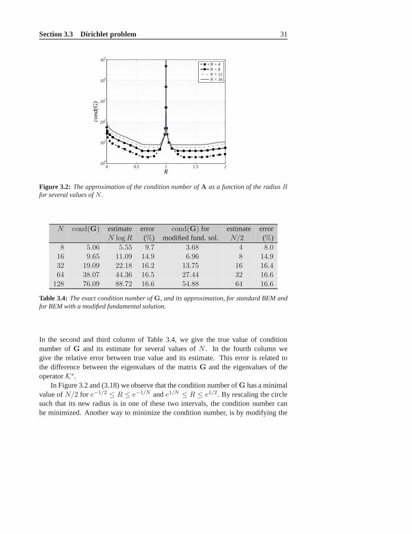
In Figure 3.2 we plot the approximation of (3.17) as a function of the radiusRfor four different values ofN : 4, 8, 12, and16. Note that the behaviour of thecondition number as shown in the figure is in good agreement with the results inliterature [19, 20]. ForR = 1 the condition number jumps to infinity. This impliesthat the linear systemGq = f is singular for the unit circle. In Chapter 4 we elaborateon modifications of the standard BEM formulation to avoid such singular systems.ForR → 0 the condition number also increases to infinity, reflecting the equationsbecoming singular when the domain shrinks to a single point.In Figure 3.2 a numberof regimes can be distinguished, in which the behaviour of the condition number isdifferent. To distinguish these regimes we write the estimate of the condition numberin (3.17) as
cond(G) ≈
12| log R| e−1/N ≤ R < 1 and1 < R ≤ e1/N ,
N2 e−1/2 ≤ R ≤ e−1/N ande1/N ≤ R ≤ e1/2,
N | logR| 0 ≤ R ≤ e−1/2 ande1/2 ≤ R <∞.
(3.18)
To study the accuracy of the approximation in (3.17), we chooseR = 2 andN ≥ 2. In that casee1/2 ≤ R <∞ and the condition number ofG is estimated by
cond(G) ≈ N log 2. (3.19)
Section 3.3 Dirichlet problem 31
0 0.5 1 1.5 210
0
101
102
103
104
105
R
con
d(G
)
N = 4N = 8N = 12N = 16
Figure 3.2: The approximation of the condition number ofA as a function of the radiusRfor several values ofN .
N cond(G) estimate error cond(G) for estimate errorN logR (%) modified fund. sol. N/2 (%)
8 5.06 5.55 9.7 3.68 4 8.016 9.65 11.09 14.9 6.96 8 14.932 19.09 22.18 16.2 13.75 16 16.464 38.07 44.36 16.5 27.44 32 16.6
128 76.09 88.72 16.6 54.88 64 16.6
Table 3.4: The exact condition number ofG, and its approximation, for standard BEM andfor BEM with a modified fundamental solution.
In the second and third column of Table 3.4, we give the true value of conditionnumber ofG and its estimate for several values ofN . In the fourth column wegive the relative error between true value and its estimate.This error is related tothe difference between the eigenvalues of the matrixG and the eigenvalues of theoperatorKs.
In Figure 3.2 and (3.18) we observe that the condition numberof G has a minimalvalue ofN/2 for e−1/2 ≤ R ≤ e−1/N ande1/N ≤ R ≤ e1/2. By rescaling the circlesuch that its new radius is in one of these two intervals, the condition number canbe minimized. Another way to minimize the condition number,is by modifying the

32 Chapter 3 Laplace equation at two-dimensional domain
fundamental solution of the Laplace operator by including afactorα,
Gα(r) =1
2πlog
(α
r
)
. (3.20)
This changes the eigenvalue−R logR of Ks to −R log(R/α). In that case theestimate for the condition number ofG becomes
cond(G) ≈ max(
12 , | logR/α|
)
min(
1N , | logR/α|
) . (3.21)
By choosingα = Re−1/2 the nominator reduces to1/2 and the denominator to1/N .As a consequence we havecond(G) ≈ N/2, which is the smallest value reached inFigure 3.2. This agrees with the theory that the condition number of the BEM-matrixfor a Laplace equation with Dirichlet conditions on any 2D domain can be minimizedtoO(N) [97]. In the last three columns of Table 3.4 we show the effectof the strategyof modifying the fundamental solution. We give the true condition number ofG withmodified fundamental solution, the corresponding estimateof N/2, and the relativeerror. We observe that the condition number for the new matrix is approximately25% smaller than the condition number of the original matrix. The most importantgain however is that the condition number does not become infinitely large anymore.
3.4 Neumann problem
In this section we study the Laplace equation on a circle withNeumann boundaryconditions. In this caseq = q is known at the whole boundary and the BIE (2.21)reduces to
(1
2I + Kd)u = f. (3.22)
Heref := Ksq is a known function depending on the boundary data. Similarly thealgebraic equations (2.30) reduce to
Hu = f , (3.23)
wheref := Gq is a known vector. As theN elements and nodes are uniformlydistributed over the boundaryΓ, the matrixH is symmetric. Hence the singularvalues of H are equal to the absolute values of the eigenvalues ofH, andconsequently
cond(H) =σmax(H)
σmin(H)=
λ1(H)
λN (H). (3.24)

Section 3.4 Neumann problem 33
0 20 40 60 80 100
10
20
30
40
50
60
70
80
90
100
110
N
con
d(H
)
~
exactestimate
Figure 3.3: The condition number ofH as a function ofN .
Note that bothλ1(H) andλN (H) are positive. As the exact eigenvalues ofH areknown andH = 1
2I + H we thus find
λ1(H) =1
2+
1
2πtan
( π
N
)
,
λN (H) =1
2− N − 1
2πtan
( π
N
)
. (3.25)
Consequently the condition number ofH is equal to
cond(H) =π + tanπ/N
|π − (N − 1) tan π/N | . (3.26)
In Figure 3.3 we show the condition number ofH as a function ofN . ForN ≥ 10,the condition number shows a strong linear behaviour inN . Realizing that for largeN we havetan π/N ≈ π/N , we find for the condition number
cond(H) ≈ π + π/N
π − (N − 1)π/N= N + 1, (3.27)
which confirms the linear behaviour from the figure.The Laplace equation with Neumann boundary conditions is inessence an ill-
posed problem. This is reflected by the zero eigenvalue of theboundary integraloperator12I +Kd; the corresponding BIE (3.22) is singular. Hence we may expect asingular system for the discrete equationsHu = f , i.e. an infinitely large condition

34 Chapter 3 Laplace equation at two-dimensional domain
number ofH. Nevertheless, the condition number ofH only grows linearly withN .This is a consequence of the discretisation of the problem. The smallest eigenvalueof the discrete problem, i.e. the smallest eigenvalue ofH, is not exactly equal tozero, but approaches zero as the discretisation of the boundary becomes finer, i.e. thenumber of elementsN increases.
3.5 Mixed boundary conditions
In this section we consider the Laplace equation on a circle with mixed boundaryconditions. We assume that the firstm elements of the boundary have Dirichletboundary conditions and the lastN − m elements Neumann conditions. We canalways reach such a situation by renumbering the elements. The BIE reads
(1
2I + Kd
)u = Ksq, (3.28)
while the set of algebraic equations is given by(1
2I + H
)u = Gq. (3.29)
As described in Section 2.3 the latter equations can be written as
Ax = f , (3.30)
where the matrixA is constructed from the matricesG andH by
A = [−GP1 | HP2]. (3.31)
In this section we derive an estimate for the condition number of the BEM-matrixA.Due to the symmetry of the boundary discretisation the matricesG andH are
circulant matrices [33]. Given the first row of such a matrix, one obtains the otherrows by a cyclic shift of the first row. An important property of a circulant matrixXis that it can be decomposed asX = F∗ΛF, whereΛ is a diagonal matrix containingthe eigenvalues ofX. The matrixF is the so-calledFourier matrix, whose elementsare defined by
F ∗lk :=
1√Nw(l−1)(k−1), (3.32)
The asterisk denotes complex conjugation andw := e2πi/N is theN -th root of unity.The Fourier matrixF is a unitary matrix. We apply the decomposition property ofcirculant matrices toG andH,
G = F∗ΛGF,
H = F∗ΛHF. (3.33)

Section 3.5 Mixed boundary conditions 35
Here ΛG and ΛH are diagonal matrices containing the eigenvalues ofG and H
respectively. Here the eigenvalues ofG are replaced by the eigenvalues ofKs andfor the eigenvalues ofH we use the exact expressions in (3.25) Substituting thedecompositions forG andH in (3.31), we writeA as
A = F∗[−ΛGFP1 | ΛHFP2]. (3.34)
We defineF1 := FP1 andF2 := FP2 to find
A = F∗[−ΛGF1 | ΛHF2]. (3.35)
By introducing two other diagonal matricesΛ and D by Λ := Λ1/2G Λ
−1/2H and
D := Λ1/2G Λ
1/2H , we obtain∗
A = F∗D[−ΛF1 | Λ−1F2]. (3.36)
We also introduce QR-decompositions ofΛF1 andΛ−1F2 as
ΛF1 = Q1U1,
Λ−1F2 = Q2U2. (3.37)
The columns ofQ1 andQ2 form bases of the subspaces which are spanned by thecolumns ofΛF1 andΛ−1F2. The matricesU1 andU2 are upper triangular matrices.With these decompositionsA can be written as
A = F∗D[
−Q1 | Q2
]
︸ ︷︷ ︸
Q
[U1 ∅∅ U2
]
︸ ︷︷ ︸
U
= F∗DQU. (3.38)
Since the unitary matrixF has condition number equal to1 we find
cond(A) ≤ cond(D) cond(Q) cond(U). (3.39)
Hence to bound the condition number ofA we need estimates of the conditionnumbers of the matricesD, Q andU.
Estimating cond(D)
The matrixD is the product of two diagonal matrices of which we can approximateor determine the singular values, namelyΛG andΛH. For convenience we list the
∗DefiningΛ andD as the square root ofΛG andΛH may yield complex numbers when a diagonalelement ofΛG or ΛH is negative. However, in order to estimate the condition numbers, we only needto evaluate thesquaredsingular values ofΛ andD, thus avoiding complex numbers.

36 Chapter 3 Laplace equation at two-dimensional domain
0 20 40 60 80 1003
4
5
6
7
8
9
N
con
d(D
)
exactestimate
Figure 3.4: Condition number ofD as a function ofN withR = 1/2 andm = N/2. Dotsrepresent the exact values while the dashed line representsthe estimate.
largest and smallest singular value ofD squared,
σ1(D)2 = σ1
(
Λ1/2G Λ
1/2H
)2= σ1 (ΛGΛH)2 = max
l[ΛGΛH ]ll
= max
R| logR|[1
2− N − 1
2πtan
π
N
]
,R
4+R
4πtan
π
N
,
σN (D)2 = σN
(
Λ1/2G Λ
1/2H
)2= σN (ΛGΛH)2 = min
l[ΛGΛH ]ll
= min
R| logR|[1
2− N − 1
2πtan
π
N
]
,R
2N+
R
2Nπtan
π
N
.
(3.40)
The condition number ofD is the square root of the ratio of these two expressions.Figure 3.4 shows the condition number ofD as a function ofN . The dots give theexact value of the condition number while the dashed line represents the estimateas constructed in this section. We observe that there is a very good correspondencebetween exact values and the estimated values.

Section 3.5 Mixed boundary conditions 37
Estimating cond(Q)
TheKantorovich-Wielandt angleθ is found by taking pairs of orthogonal vectorsx
andy and calculating the smallest angle between their images underQ [48],
cos θ := maxx⊥y
|(Qx,Qy)|‖Qx‖‖Qy‖ . (3.41)
The condition number ofQ is related to the Kantorovich-Wielandt angle by
cond(Q) = atan(θ/2), (3.42)
It can be proven that the angleθ is the angle between the two subspaces spanned bythe columns ofΛF1 andΛ−1F2.
Lemma 3.1 The Kantorovich-Wielandt angleθ is equal to the angle between the twosubspaces spanned by the columns ofΛF1 andΛ−1F2.
Proof. The angleα between the two subspaces that are spanned by the columns ofΛF1 andΛ−1F2 is defined as [8]
cosα := maxξ1∈R(ΛF1)
maxξ2∈R(Λ−1F2)
|(ξ1, ξ2)|‖ξ1‖‖ξ2‖
. (3.43)
To evaluate the Kantorovich-Wielandt angle we realize the following. The matrixQconsists of two blocks, and therefore we select two special vectorsx andy, namelyx = [xT
1 | 0, . . . , 0]T andy = [0, . . . , 0 | yT1 ]T , wherex1 ∈ R
m andy1 ∈ RN−m.
Clearly we havex ⊥ y. Moreover, we observe thatQx = −Q1x1 andQy = Q2y1.We substitute this into the definition of the Kantorovich-Wielandt angle and find
cos θ = maxx1∈Rm
maxy1∈RN−m
|(Q1x1,Q2y1)|‖Q1x1‖‖Q2y1‖
. (3.44)
Recall that the columns of the matricesQ1 andQ2 form an orthogonal basis forthe subspaces spanned by the columns ofΛF1 andΛ−1F2. This means that we canintroduceξ1 ∈ R(ΛF1) andξ2 ∈ R(Λ−1F2) such thatξ1 = Q1x1 andξ2 = Q2y1.Then (3.44) becomes
cos θ = maxξ1∈R(ΛF1)
maxξ2∈R(Λ−1F2)
|(ξ1, ξ2)|‖ξ1‖‖ξ2‖
, (3.45)
which is the definition of the angle between the subspaces. Thus the Kantorovich-Wielandt angleθ is equal to the angleα between the two subspaces.

38 Chapter 3 Laplace equation at two-dimensional domain
Lemma 3.1 is used to prove the following theorem.
Theorem 3.2 The condition number ofQ is equal to1.
Proof. The angleθ can be calculated from
cos θ = maxx∈R(ΛF1)
maxy∈R(Λ−1F2)
|(x,y)|‖x‖‖y‖
= maxx∈R(F1)
maxy∈R(F2)
|(Λ−1x,Λy)|‖Λ−1x‖‖Λy‖
= maxx∈R(F1)
maxy∈R(F2)
|(Λ∗Λ−1x,y)|‖Λ−1x‖‖Λy‖ . (3.46)
For 0 < R ≤ 1, Λ is a diagonal matrix with real elements, henceΛ∗ = Λ, and wefind
cos θ = maxx∈R(F1)
maxy∈R(F2)
|(x,y)|‖Λ−1x‖‖Λy‖ . (3.47)
However, sinceR(F1) ⊥ R(F2), the inner product between the vectorsx ∈ R(F1)andy ∈ R(F2) is equal to zero. Hencecos θ = 0 and consequentlycond(Q) = 1.
For R > 1, the first diagonal element ofΛG is negative, and hence the firstdiagonal element ofΛ = Λ
1/2G Λ
−1/2H is imaginary. In that case
(Λ−1x,Λy) =
(
− i
a1
)
(ia1)x1y1 + x2y2 + . . .+ xNyN = 0, (3.48)
whereaj , j = 1, . . . , N , are the diagonal elements ofΛ. So also in the caseR > 1cos θ = 0 andcond(Q) = 1.
Since the condition number ofQ is equal to one, it is interesting to note thatQ isa unitary matrix.
Corollary 3.3 The matrixQ is unitary.
Proof. Recall that the matrixQ consists of a unitaryN×m blockQ1 and a unitaryN× (N −m) blockQ2. Accordingly we can split any vectorx ∈ R
N into two parts,x = [xT
1 ;xT2 ]T . The matrix-vector productQ∗Qx then reads
Q∗Qx =
[x1 − Q∗
1Q2x2
−Q∗2Q1x1 + x2
]
. (3.49)
The subspaces that are spanned by the columns ofΛF1 and Λ−1F2 areperpendicular. The matricesQ1 and Q2 are bases of these subspaces, andconsequentlyQ∗
1Q2 = Q∗2Q1 = 0. Thus we findQ∗Qx = x. Likewise we can
prove thatQQ∗x = x. HenceQ∗Q = QQ∗ = I andQ is a unitary matrix.

Section 3.5 Mixed boundary conditions 39
Estimating cond(U)
To estimate the condition number ofU we need estimates of the singular values ofU1 andU2. For this observe that
σk(U1) = σk(Q1U1) = σk(ΛF1) ≤ σk(Λ)σ1(F1) = σk(Λ),
σk(U2) = σk(Q2U2) = σk(Λ−1F2) ≤ σk(Λ
−1)σ1(F2) = σk(Λ−1),
(3.50)
for k = 1, . . . ,m andk = 1, . . . , N −m respectively. Here we used the facts thatQi andFi have orthogonal columns and have singular values1. We also made useof estimates of the singular values of products of matrices [47]. Furthermore, withF1 = Λ−1Q1U1 andF2 = ΛQ2U2 we obtain
1 = σk(F1) = σk(Λ−1Q1U1) ≤ σ1(Λ
−1)σk(Q1U1) = σ1(Λ−1)σk(U1),
1 = σk(F2) = σk(ΛQ2U2) ≤ σ1(Λ)σk(Q2U2) = σ1(Λ)σk(U2),
(3.51)
for k = 1, . . . ,m andk = 1, . . . , N − m respectively. This yields the followinglower bounds,
σk(U1) ≥ 1
σ1(Λ−1)
= σN (Λ), k = 1, . . . ,m,
σk(U2) ≥ 1
σ1(Λ)= σN (Λ−1), k = 1, . . . , N −m. (3.52)
With (3.50) and (3.52) we have upper and lower bounds for the singular values ofU1 andU2. The singular values ofU are the singular values ofU1 plus the singularvalues ofU2, i.e. σ(U) = σ(U1)
⋃σ(U2). For the condition number ofU we
obtain
cond(U) =σ1(U)
σN (U)≤ max
σ1(Λ), σ1(Λ
−1)
minσN (Λ), σN (Λ−1)
=
max
σ1(Λ), 1σN (Λ)
min
σN (Λ), 1σ1(Λ)
= max
σ1(Λ)2,1
σN (Λ)2
. (3.53)

40 Chapter 3 Laplace equation at two-dimensional domain
0 20 40 60 80 1000
20
40
60
80
100
120
N
con
d(U
)
exactestimate
Figure 3.5: Condition number ofU as a function ofN , whereR = 1/2 andm = N/2. Thedashed line is the estimate whereas the large dots give the exact value for several values ofN .
SinceΛ is the product of the square roots ofΛG andΛ−1H , we can derive its singular
values, resulting in
σ1(Λ)2 = max
2πR| logR|
π − (N − 1) tan π/N,
πR
π + tan π/N
,
σN (Λ)2 = min
2πR| logR|
π − (N − 1) tan π/N,
2πR/N
π + tanπ/N
. (3.54)
We plot the condition number ofU and its approximation in Figure 3.5. Asis seen from (3.53), the approximation provides an upper bound for the conditionnumber ofU. The difference between the exact value and the estimate corresponds tothe error that is made by approximating the smallest eigenvalue ofG by the smallesteigenvalue ofKs.
Estimating cond(A)
The condition number ofA is estimated by the product of condition numbers ofD
andU, where the condition number ofU is obtained from the singular values ofΛ.Let us use a first order approximation fortan π/N to approximate the largest andsmallest singular values of the matricesD andΛ as given in (3.40) and (3.54). We

Section 3.5 Mixed boundary conditions 41
find
σ1(D)2 ≈ R
4Nmax
(2| logR|, N + 1
),
σN (D)2 ≈ R
2Nmin
(
| logR|, 1 +1
N
)
,
σ1(Λ)2 ≈ RN max(
2| logR|, 1
N + 1
)
,
σN (Λ)2 ≈ 2RN min(
| logR|, 1
N(N + 1)
)
. (3.55)
For a circle with radiusR = 1/2 we obtain
cond(D) ≈√
N + 1
2 log 2,
cond(U) . N + 1, (3.56)
wich gives the following estimate for the condition number of A,
cond(A) .1√
2 log 2(N + 1)3/2. (3.57)
Figure 3.6 shows this estimate for the condition number. Thedashed line givesthe estimate as a function ofN , whereas the dots give the exact value of the conditionnumber for several values ofN . For this example we choosem = N/2, i.e. as manyelements with Dirchlet conditions as elements with Neumannconditions. However,the parameterm does not appear in the estimates, and will not play any role. Weobserve that the estimate is of higher order than the actual value of the conditionnumber. In fact the condition number ofA turns out to be linear inN , while theestimate is of orderN3/2. Later on we will show how this discrepancy is caused.
Figure 3.7 gives the condition number ofA and its estimate as a function ofR.We chooseN = 12 andm = 6. Again the estimate isO(N3/2), while the actualvalue isO(N). The estimate does capture the large condition number atR = 1though.
Let us recapitulate the steps that we have taken to bound the condition numberof the matrixA. We decomposedA in a product of matrices and derived thatcond(A) ≤ cond(D)cond(U). We can evaluate or approximate the conditionnumbers ofD andU very well, but the condition number ofA is over-estimated.This must be caused by the decomposition ofA. As a simple example, consider thematricesX andY, given by
X :=
[1 00 ε
]
, Y :=
[1 00 1/ε
]
, (3.58)

42 Chapter 3 Laplace equation at two-dimensional domain
0 20 40 60 80 10010
0
101
102
103
N
con
d(A
)
exactestimate
Figure 3.6: Condition number ofA as a function ofN , whereR = 1/2 andm = N/2. Thedashed line is the estimate whereas the large dots give the exact condition number for severalvalues ofN .
0 0.5 1 1.5 2 2.5 3 3.5 410
0
101
102
103
104
105
con
d(A
)
R
exactestimate
Figure 3.7: Condition number ofA as a function ofR, whereN = 12 andm = 6. Thedashed line is the estimate whereas the large dots give exactvalues for several values ofR.

Section 3.6 Decoupled equations 43
where0 < ε≪ 1. Clearly both matrices have a large condition number∼ ε−1, whilethe product matrixZ := XY has condition number1. Exploiting the fact thatZ is aproduct ofX andY yields,
cond(Z) ≤ cond(X)cond(Y) =1
ε2, (3.59)
which highly over-estimates the condition number ofZ. Thus decomposing amatrix and multiplying the condition numbers of the severalfactor matrices doesnot nessecarily yield a good approximation of the conditionnumber of the originalmatrix.
3.6 Decoupled equations
The decomposition of the BEM-matrixA that we derived in the previous sectionhas been useful for finding an estimate for the condition number of A. Besides thisestimate the decomposition can also be used to decouple the equations from the BEMformulation. This allows us to separately retrieve the missing information ofu atΓ2
andq at Γ1. Recall equation (2.37), relating the boundary datab to the unknownvectorx,
Ax = Gb. (3.60)
In the previous section we have shown thatA is decomposed as
A = F∗DQU. (3.61)
The matrixG can be decomposed in a smiliar manner. First we writeG as
G = [−HP1 | GP2]
= [−F∗ΛHFP1 | F∗ΛGFP2]
= F∗[−ΛHF1 | ΛGF2]
= F∗D[−Λ−1F1 | ΛF2]. (3.62)
Realizing that the vectorb is constructed from the boundary datau1 andq2, namelyb = [u1; q2], we can write the right-hand side of (3.60) as
Gb = F∗D(−Λ−1F1u1 + ΛF2q2
)=: F∗D f . (3.63)
Using the new expressions forA andGb, equation (3.60) becomes
F∗DQUx = F∗Df . (3.64)

44 Chapter 3 Laplace equation at two-dimensional domain
Multiplying by Q∗D−1F yields
Ux = Q∗f , (3.65)
or[
U1 ∅∅ U2
] [q1
u2
]
= [−Q1 | Q2]∗f =
[−Q∗
1f
Q∗2f
]
. (3.66)
So we obtain a set of two linear systems,
U1q1 = −Q∗1f , (3.67a)
U2u2 = Q∗2f . (3.67b)
We are given datau1 on Γ1 andq2 on Γ2. Assume that we are interested inu2, i.e.the unknown coefficients ofu atΓ2. In the original BEM formulation we would thencalculate bothu atΓ2 andq atΓ1. With equation (3.67b) we can directly calculateuatΓ2 without computingq atΓ1.
Let us summarize which steps we have to take in order to compute u at Γ2.First we need the Fourier matrixF, whose two componentsF1 andF2 appear inthe vectorf . We also need the diagonal matrixΛ, which contains the eigenvaluesof the matricesG andH (Λ = Λ
1/2G Λ
−1/2H ). These eigenvalues are approximated
by the eigenvalues of the single and double-layer potentials. Then we need a QR-decomposition of the matrix productΛ−1F2, which yields us the matricesQ2 andU2. Finally we solve the system in (3.67b). Note that the matrixU2 in this systemis an upper triangular matrix, so the system is solved very efficiently by backwardelimination. The most costly step in this procedure is the QR-decomposition ofΛ−1F2. However, note thatΛ−1F2 is aN × (N − m) matrix. With the originalBEM procedure we would have to find a QR-decomposition for aN ×N matrix.
The method described above works similarly if we want to calculate q at Γ1
without computingu at Γ2. Then we need a QR-decomposition forΛF1 and solveequation (3.67a).
Example 3.1
Consider the following problem on the circleΩ with radiusR,
∇2u = 0, x ∈ Ω,u = R cos θ, x ∈ Γ1,q = cos θ, x ∈ Γ2,
(3.68)
which has exact solutionu = R cos θ and q = cos θ at Γ. We chooseR = 2,m = N − 1, so all elements have Dirichlet boundary conditions, except for the lastelement. We calculate the value ofu in this last element, following the procedure

Section 3.6 Decoupled equations 45
BEM BEM decoupled
N time(s) rel. error time(s) rel. error
100 0.44 3.93 · 10−4 0.10 3.96 · 10−4
200 1.85 9.95 · 10−4 0.39 9.95 · 10−5
300 4.56 4.44 · 10−5 1.27 4.43 · 10−5
400 9.14 2.51 · 10−5 2.97 2.49 · 10−5
500 15.80 1.61 · 10−5 5.64 1.60 · 10−5
Table 3.5: Calculation time and relative error for both BEM and decoupled BEM. Problemthat is solved is almost purely Dirichlet (m = N − 1).
BEM BEM decoupled
N time (s) time (s)
100 0.43 0.12
200 1.82 0.56
300 4.63 1.86
400 9.13 4.08
500 15.80 7.79
Table 3.6: Calculation time for both BEM and decoupled BEM. Problem that is solved hasmixed boundary conditions (m = N/2).
described above. In Table 3.5 we see that the computation time for findingu with thedecoupled BEM is a factor3 to 4 lower than findingu with the original BEM. At thesame time the accuracy is equally good.
Now let us choosem = N/2 and calculateu at Γ2 andq at Γ1 separately usingthe decoupled BEM and compare this to the original BEM. The computation time isgiven in Table 3.6. Again we see that the decoupled BEM is faster than the originalBEM. The reason for this is simple: it is more efficient to solve two small systemsthan one large system.
We can improve the efficiency even more, as we do not need to solve the systemsin (3.67) by backward elimination. For this we multiply (3.67a) byQ1,
Q1U1q1 = −Q1Q∗1f , (3.69)

46 Chapter 3 Laplace equation at two-dimensional domain
and replace the productQ1U1 by ΛF1,
ΛF1q1 = −Q1Q∗1f . (3.70)
We next multiply byF∗1Λ
−1 to find
q1 = −F∗1Λ
−1Q1Q∗1f . (3.71)
The linear system in (3.67b) can be transformed in a similar manner, and the twosystems in (3.67) are solved with
q1 = −F∗1Λ
−1Q1Q∗1f , (3.72a)
u2 = F∗2ΛQ2Q
∗2f . (3.72b)
In this wayq1 andu2 are found without using backward substitution. Neverthelessthe expressions on the right-hand sides involve many matrix-vector multiplicationsand may therefore be not very efficient. Moreover we still need to findQ1 andQ2,i.e. perform QR-decompositions.
For a pure Dirichlet problem, i.e.m = N , we haveQ1 = Q, which is a unitarymatrix. Therefore the matrix productQ1Q
∗1 in (3.72a) is equal to theN ×N matrix
IN . Also PT1 = IN and the vectorf is equal tof = −Λ−1Fu. Hence, for the
Dirichlet problem (3.72a) becomes
q = −F∗Λ−1(−Λ−1Fu) = F∗Λ−2Fu = F∗Λ−1G ΛHFu. (3.73)
All matrices in this expression are known or can be approximated accurately. Thuswe obtainq by performing a simple matrix-vector product. In a similar manner wefind u from boundary dataq with
u = F∗ΛGΛ−1H Fq. (3.74)

Chapter 4
Logarithmic capacity
In this chapter we investigate the uniqueness of the solution of the boundary integralequation (BIE) for the Laplace equation on a general two-dimensional domain.Three different types of boundary conditions are distinguished: Dirichlet, mixedand Neumann boundary conditions. For a Laplace equation with Dirichlet boundaryconditions it has been shown that a unique solution does not always exist, dependingon the size of the domain. A similar result is proven for the case of mixed boundaryconditions. The BIE for the Laplace equation with Neumann boundary conditionsdoes never have a unique solution.
4.1 Introduction
It is well-known that the Laplace equation in differential form with either Dirichletor mixed boundary conditions has a unique solution. However, when the Laplaceequation is transformed to a BIE this is not so straightforward anymore. It is notedthat the BIE for the Dirichlet Laplace equation does not always have a unique solution[53, 56, 75, 85]. Certain domains can be distinguished on which the BIE becomessingular and a non-trivial solution of the homogeneous equations can be found.A multiple of this solution can be added to the solution of thenon-homogeneousequations, which is then no longer unique. For each domain there exists exactly onerescaled version of this domain for which the BIE becomes singular. This introducesan extraordinary phenomenon for the BIEs; uniqueness of thesolutions depends onthe scale of the domain.
The domains on which no unique solution can be guaranteed arerelated to theso-calledlogarithmic capacity. The logarithmic capacity is a real positive numberbeing a function of the domain. This concept originates fromthe field of measuretheory, but it also appears in potential theory. The conceptof a capacity applied to
47

48 Chapter 4 Logarithmic capacity
a single domain may be a bit confusing, as usually theelectrical capacity is definedas a charge difference between two conducting objects. The logarithmic capacityhowever is related to a single domain.
In potential theory it is shown that when the logarithmic capacity of a domainis equal to one, then the homogeneous BIE for the Dirichlet Laplace equation at theboundary of that domain has a non-trivial solution [52, 66, 91]. This allows us toa-priori detect whether a BIE will become singular on a certain domain. Namely,we have to compute the logarithmic capacity and verify whether it is equal to one.Additionally, the logarithmic capacity also enables us to modify the BIE such that itdoes not become singular. We can scale the domain in such a waythat the logarithmiccapacity does not become equal to one. The BIE on the corresponding boundary willthen be nonsingular.
The BIE for the Laplace equation with mixed boundary conditions did not receivemuch attention until now [39]. However, a similar phenomenon as for the Dirichletcase takes place for mixed conditions. For each domain thereexists exactly onerescaled version of this domain for which the BIE becomes singular. This result isproven in Section 4.4.
Research has been done on the BIE for the biharmonic equation. It is shown thatthe BIE for the biharmonic equation with Dirichlet conditions on a circle does notadmit a unique solution when the radius of the circle is equalto 1 or e−1 [23]. A fewyears later it was shown that a more general result is true: for any 2D domain thereexists two critical scalings for which the BIE does not have aunique solution [44].For the BIE for the biharmonic equation, the number of critical scaling can evenincrease to three or four for domains that consist of two or four separate squares [30].Apart from rescaling the domain there are two options to guarantee nonsingular BIEsand a unique solution. The first option is to add two supplementary conditions [23],while the second option involves modified fundamental solutions for the biharmonicequation [28].
Another class of BIEs for which uniqueness properties has been investigated isthe class of BIEs for the Helmholtz equation. It is derived that there is a countableset of critical wave numbers for which the condition number of both the integraloperator as the related discrete operator becomes infinitely large [2, 59, 60, 61]. Byintroducing a coupling parameter between the various boundary integral operatorsit is shown that the condition numbers can be minimized. The singular BIE forthe Helmholtz equation is different from the singular BIEs for the Laplace andbiharmonic equation. The singularity appears at certain wave numbers, and notat certain critical scalings. Moreover singular BIEs also appear for the Helmholtzequation in 3D. This is not the case for the BIEs for the Laplace and biharmonicequation.
In this chapter we investigate both the BIE for the Laplace equation with Dirichlet

Section 4.1 Introduction 49
conditions and mixed conditions, and we also include the BIEfor the Laplaceequation with Neumann conditions. Thus we study three different problems. Firstwe describe the setting of these three problems.
Let Ω be a simply connected domain in 2D whose boundaryΓ is a closed curve.In the interior ofΩ the Laplace equation holds for the unknown functionu = u(x),
∇2u = 0, x ∈ Ω. (4.1)
Recall that thefundamental solutionG of the Laplace operator∇2 is given by
G(x,y) :=1
2πlog
1
‖x− y‖ . (4.2)
We denote byq the derivative ofu with respect to the outward normaln at Γ.Introduce thesingle and double layer potentialby
(Ksq)(x) :=
∫
ΓG(x,y)q(y)dΓy, x ∈ Γ,
(Kdu)(x) :=
∫
Γ
∂
∂nyG(x,y)u(y)dΓy, x ∈ Γ, (4.3)
respectively. The BIE for the Laplace equation deduced in Chapter 2 reads (cf. [6])
1
2u+ Kdu = Ksq, x ∈ Γ. (4.4)
At each point on the boundary we prescribe eitheru or q. We distinguish three typesof boundary conditions.Dirichlet problem
u = u, x ∈ Γ. (4.5)
Mixed problem
u = u, x ∈ Γ1,
q = q, x ∈ Γ2, (4.6)
Neumann problem
q = q, x ∈ Γ. (4.7)
whereΓ1 ∪ Γ2 = Γ andΓ1 ∩ Γ2 = ∅.

50 Chapter 4 Logarithmic capacity
4.2 Logarithmic capacity
To study the uniqueness properties of the Dirichlet and the mixed problem in the nextsection we need to introduce the notion oflogarithmic capacity. We define the energyintegralI by
I(q) :=
∫
Γ
∫
Γlog
1
‖x− y‖q(x)q(y)dΓxdΓy (4.8)
and the logarithmic capacityCl(Γ) is related to this integral by
− logCl(Γ) := infqI(q). (4.9)
Here the infimum is taken over all functionsq with the restriction that∫
Γq(x)dΓx = 1. (4.10)
Let us give a physical interpretation of the logarithmic capacity. For simplicitylet the domainΩ be contained in the disc with radius1/2. In that case it can be shownthat the integralI(q) is positive. The functionq can be seen as a charge distributionover a conducting domainΩ. Faraday demonstrated that this charge will only resideat the exterior boundary of the domain, in our case atΓ. We normalizeq in such away that the total amount of charge atΓ is equal to one, cf. condition (4.10). ThefunctionKsq is identified as the potential due to the charge distributionq. Note thatthe integralI can also be written as
I(q) = 2π
∫
Γ(Ksq)(x)q(x)dΓx. (4.11)
HenceI can be seen as the energy of the charge distributionq. The charge willdistribute itself overΓ in such a way that the energyI is minimized. So the quantity− logCl(Γ) is the minimal amount of energy. Hence the logarithmic capacity Cl(Γ)is a measure for the capability of the boundaryΓ to support a unit amount of charge.
For most boundaries the logarithmic capacity is not known explicitly. Only for afew elementary domains the logarithmic capacity can be calculated analytically [66];we have listed some in Table 4.1.
There are also some useful properties [5, 52] that help us to determine or estimatethe logarithmic capacity.
1. If Γ is the outer boundary of a closed bounded domainΩ, thenCl(Γ) = Cl(Ω).This agrees with the idea of Faraday’s cage, mentioned above.
2. Denote bydΓ the Euclidean diameter ofΩ, thenCl(Γ) ≤ dΓ. Hence theradius of the smallest circle in whichΓ is contained is an upper bound for thelogarithmic capacity ofΓ.

Section 4.3 Dirichlet problem 51
boundaryΓ logarithmic capacityCl(Γ)
circle with radiusR R
square with sideLΓ( 1
4)2
4π3/2 L ≈ 0.59017 · Lellipse with semi-axesa andb (a+ b)/2
interval of lengtha 14a
isosceles right triangle sidel 33/4Γ(1/4)2
27/2π3/2 l ≈ 0.476 l
Table 4.1: The logarithmic capacity of some domains. Note thatΓ(·) represents the gamma-function.
3. If Γ = x + αΓ1, thenCl(Γ) = αCl(Γ1). Hence the logarithmic capacitybehaves linearly with respect to scaling and is invariant with respect totranslation.
4. If Ω1 ⊂ Ω2, thenCl(Ω1) ≤ Cl(Ω2).
5. For a convex domainΩ,
Cl(Ω) ≥(
area(Ω)
π
)1/2
. (4.12)
If the properties from the list above do not supply accurate enough estimates, thelogarithmic capacity can also be approximated numericallywith the help of linearprogramming [82].
4.3 Dirichlet problem
For the BIE that arises from the Laplace equation with Dirichlet boundary conditionswe have the following result.
Theorem 4.1 There exists a nonzeroqe such that
(Ksqe)(x) = − 1
2πlogCl(Γ), x ∈ Γ. (4.13)
Sketch of proof. In the following we briefly present the major steps in the proof ofthe theorem [52, 70, 98]. We observe that for the values of theenergy integral (4.8)we have−∞ < I(q) ≤ ∞. If the infimum of the energy integral is infinitely large,then by definition the logarithmic capacity is equal to zero.

52 Chapter 4 Logarithmic capacity
Suppose thatCl(Γ) > 0 and thus−∞ < I(q) <∞. It is proven [52, p. 282] that foreach boundaryΓ there exists a unique minimizerqe of I(q), i.e.
I(qe) = infqI(q) = − logCl(Γ) with
∫
Γqe(x)dΓx = 1. (4.14)
For the minimizerqe the following result is proven [52, p. 287]. LetΓ be a closedbounded domain with positive logarithmic capacity and a connected complement.Then2πKsqe ≤ − logCl(Γ) in the whole plane and2πKsqe = − logCl(Γ) at Γ,except possibly for a subset which has zero logarithmic capacity.
Theorem 4.1 leads to the following result.
Corollary 4.2 If Cl(Γ) = 1 there exists a nonzeroqe such thatKsqe = 0.
Thus in the specific case thatCl(Γ) = 1 the single layer operatorKs admits aneigenfunctionqe with zero eigenvalue. HenceKs is not positive definite and theDirichlet problem does not have a unique solution.
If we rescale the domain such that the Euclidean diameter is smaller than one,then the second property in Section 4.2 shows us that the logarithmic capacity willalso be smaller than one. In this way we can guarantee the existence of a uniquesolution of the BIE.
Recall that the non-trivial solutionqe of the homogeneous BIEKsq = 0 has acontour integral equal to1. At the same time we realize that a solutionq of Ksq = 0has to satisfy
∫
ΓqdΓ =
∫
Ω∆udΩ = 0, (4.15)
where we make use of Gauss’ theorem. By adding this requirement for q to the BIE,we exclude the possibility thatqe is a solution of the homogeneous BIE. This providesa second strategy to ensure unique solutions of the BIE.
A third option to guarantee a unique solution is to adjust theintegral operatorKs.Note that the functionGα,
Gα(x,y) :=1
2πlog
α
‖x− y‖ , α ∈ R+, (4.16)
is also a fundamental solution for the Laplace operator. Thecorresponding singlelayer potential reads
Ksαq :=
1
2π
∫
Γlog
α
‖x− y‖q(y)dΓy = Ksq +log α
2π
∫
ΓqdΓ. (4.17)

Section 4.4 Mixed problem 53
For the minimizerqe we get
Ksαqe = Ksqe +
logα
2π
∫
ΓqedΓ = − 1
2πlogCl(Γ) +
1
2πlogα
=1
2πlog
α
Cl(Γ). (4.18)
This is only equal to zero ifα = Cl(Γ). We may chooseα any positive real numberunequal toCl(Γ) and obtainKs
αqe 6= 0. In that caseqe is no longer an eigenfunctionof the single layer potential operator with zero eigenvalue. Hence the BIE (4.4) withDirichlet conditions is uniquely solvable ifKs is replaced byKs
α [26, 70]. Theadvantage of this procedure is that we do not need a rescalingof the domain, nordo we have to add an extra equation. Furthermore, we do not need to know thelogarithmic capacity explicitly; a rough estimate of the capacity sufficies to chooseαsuch thatα 6= Cl(Γ).
There are also ways to ensure a unique solution of the BIE for the Laplaceequation tha can be used without having to know the logarithmic capacity. Forinstance, adding an extra collocation node at the interior or exterior of the domaincan change the BIE in such a way that it is not singular any longer [17]. This doesdepend on the location of the extra collocation node though.Another option is to usethe hypersingular formulation of the BIE [18]. The hypersingular BIE is the normalderivative of the standard BIE and does not involve the single layer operator. As aconsequence the BIE does not become singular at certain domains.
4.4 Mixed problem
To investigate the Laplace equation with mixed boundary conditions we have torewrite the BIE in (4.4). Fori = 1, 2 we introduce the functionsui := u|Γi andqi := q|Γi and the boundary integral operators
(Ksi q)(x) :=
∫
Γi
G(x,y)q(y)dΓy, x ∈ Γ, (4.19a)
(Kdi u)(x) :=
∫
Γi
∂
∂nyG(x,y)u(y)dΓy, x ∈ Γ. (4.19b)
Note that the boundary conditions (4.6) provideu1 = u and q2 = q. Bydistinguishingx ∈ Γ1 andx ∈ Γ2, we write (4.4) as a system of two BIEs,
Kd2u2 −Ks
1q1 = Ks2q −
1
2u−Kd
1u, x ∈ Γ1, (4.20a)
1
2u2 + Kd
2u2 −Ks1q1 = Ks
2q −Kd1u, x ∈ Γ2. (4.20b)

54 Chapter 4 Logarithmic capacity
In this system all prescribed boundary data are at the right-hand side of the equations.
Theorem 4.3 If Cl(Γ) = 1, the homogeneous equations of (4.20a) and (4.20b) havea non-trivial solution pair(q1, u2).
Proof. We have to find a non-trivial pair of functions(q1, u2) such that the left-hand sides of (4.20a) and (4.20b) are equal to zero whenCl(Γ) = 1. To this end wechooseu2 ≡ 0 andq1 = qe|Γ1
+ h1, with the functionh1 satisfying
Ks1h1 = Ks
2qe, x ∈ Γ. (4.21)
With these choices both the left-hand sides of (4.20a) and (4.20b) are equal to
−Ks1q1 = −(Ks
1qe + Ks1h1) = −(Ks
1qe + Ks2qe) = −Ksqe
=1
2πlogCl(Γ) = 0. (4.22)
We still have to prove that it is possible to find a functionh1 that satisfies (4.21). Firstwe note that the right-hand side of (4.21) is in〈qe〉⊥, since
(Ks2qe, qe)Γ =
∫
Γ
∫
Γ2
G(x,y)qe(y)dΓyqe(x)dΓx
=
∫
Γ2
∫
ΓG(x,y)qe(x)dΓxqe(y)dΓy
= (Ksqe, qe)Γ2= − 1
2πlogCl(Γ)(1, qe)Γ2
= 0. (4.23)
Here(·, ·)Γ stands for the inner product over the boundaryΓ. As the right-hand sideof (4.21) is in〈qe〉⊥, we can generalize the question: is it possible to find a functionh1 such thatKs
1h1 = φ for all φ ∈ 〈qe〉⊥? If so, thenφ = Ks2qe completes the proof.
For all functionsq ∈ 〈qe〉⊥ with q 6= 0 we haveI(q) > I(qe), sinceqe is theunique minimizer ofI. UsingI(q) = 2π(Ksq, q) we find that
(Ksq, q) >1
2πI(qe) = − 1
2πlogCl(Γ) = 0, q ∈ 〈qe〉⊥, q 6= 0. (4.24)
SoKs is positive definite and invertible on the function space〈qe〉⊥. This means thatfor all φ ∈< qe >
⊥ there is a functionh with Ksh = φ. Let h be the solution ofKsh = φ, then it can be decomposed as
h =
h1, x ∈ Γ1,h2, x ∈ Γ2.
(4.25)
Recall that we search for a functionh1 such thatKs1h1 = φ, for φ ∈ 〈qe〉⊥. We add
the functionKs2h2 to this equation,
Ks1h1 + Ks
2h2 = φ+ Ks2h2, (4.26)
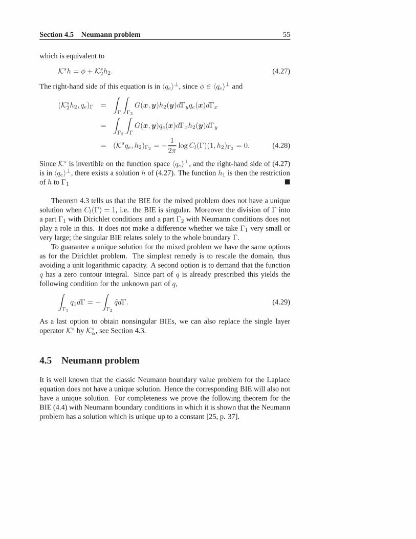
Section 4.5 Neumann problem 55
which is equivalent to
Ksh = φ+ Ks2h2. (4.27)
The right-hand side of this equation is in〈qe〉⊥, sinceφ ∈ 〈qe〉⊥ and
(Ks2h2, qe)Γ =
∫
Γ
∫
Γ2
G(x,y)h2(y)dΓyqe(x)dΓx
=
∫
Γ2
∫
ΓG(x,y)qe(x)dΓxh2(y)dΓy
= (Ksqe, h2)Γ2= − 1
2πlogCl(Γ)(1, h2)Γ2
= 0. (4.28)
SinceKs is invertible on the function space〈qe〉⊥, and the right-hand side of (4.27)is in 〈qe〉⊥, there exists a solutionh of (4.27). The functionh1 is then the restrictionof h to Γ1
Theorem 4.3 tells us that the BIE for the mixed problem does not have a uniquesolution whenCl(Γ) = 1, i.e. the BIE is singular. Moreover the division ofΓ intoa partΓ1 with Dirichlet conditions and a partΓ2 with Neumann conditions does notplay a role in this. It does not make a difference whether we take Γ1 very small orvery large; the singular BIE relates solely to the whole boundaryΓ.
To guarantee a unique solution for the mixed problem we have the same optionsas for the Dirichlet problem. The simplest remedy is to rescale the domain, thusavoiding a unit logarithmic capacity. A second option is to demand that the functionq has a zero contour integral. Since part ofq is already prescribed this yields thefollowing condition for the unknown part ofq,
∫
Γ1
q1dΓ = −∫
Γ2
qdΓ. (4.29)
As a last option to obtain nonsingular BIEs, we can also replace the single layeroperatorKs by Ks
α, see Section 4.3.
4.5 Neumann problem
It is well known that the classic Neumann boundary value problem for the Laplaceequation does not have a unique solution. Hence the corresponding BIE will also nothave a unique solution. For completeness we prove the following theorem for theBIE (4.4) with Neumann boundary conditions in which it is shown that the Neumannproblem has a solution which is unique up to a constant [25, p.37].

56 Chapter 4 Logarithmic capacity
WG
n
xB ' eB ee
Figure 4.1: The pointx ∈ Γ is the center of a small circleBε with radiusε.
Theorem 4.4 For any closed curveΓ
(1
2I + Kd
)1 = 0. (4.30)
Proof. To show that operator12I + Kd applied to the constant function1 yieldszero, we need to prove thatKd1 ≡ −1
2 at the boundary. Letx be a point at theboundaryΓ, then using Gauss’ theorem we find
(Kd1
)(x) =
∫
Γ
∂
∂nyG(x,y)dΓy =
∫
Ω∇2
yG(x,y)dΩy, (4.31)
where the subscripty means integration or differentiation with respect toy. Thefundamental solution is defined such that∇2
yG(x,y) = −δ(x − y). Hence, whenintegrating overy, we have to take special care at the pointy = x. LetBε be a smallcircle with radiusε around the pointx and letB′
ε be the part of that circle that liesinsideΩ, i.e.B′
ε = Bε ∩Ω, see Figure 4.1. The domain integral in (4.31) can be splitin
(Kd1
)(x) =
∫
Ω/B′
ε
∇2yG(x,y)dΩy +
∫
B′
ε
∇2yG(x,y)dΩy. (4.32)
Within the domainΩ/B′ε the fundamental solution does not have a singular point
and thus∇2yG(x,y) = 0 in this domain. As a consequence the first integral at the
right-hand side of (4.32) is equal to zero. If the boundaryΓ is smooth enough, thecircleB′
ε is half the size of the circleBε. Likewise, ifε goes to zero, the integral overB′
ε in (4.32) is half the size of the same integral overBε. Hence we obtain
(Kd1
)(x) =
1
2
∫
Bε
∇2yG(x,y)dΩy. (4.33)

Section 4.6 Examples 57
We use Gauss’ theorem to transform the domain integral overBε to a boundaryintegral overΓε, the boundary of the circleBε,
(Kd1
)(x) =
1
2
∫
Γε
∂
∂nyG(x,y)dΓy. (4.34)
We introduce polar coordinates(r, θ) at the circleBε, the point x being thelocal origin. Recall the definition of the fundamental solution (4.2) in which now‖x− y‖ ≡ r for y ∈ Bε. It is straightforward to see that
∂
∂nyG(x,y) =
1
2π
∂
∂rlog
1
r= − 1
2π
1
r. (4.35)
Substituting this in the integral of (4.34) results in
(Kd1
)(x) = −1
2
∫ 2π
0
1
2π
1
rrdθ = −1
2. (4.36)
The direct consequence of this is that
(1
2I + Kd
)1 = 0, (4.37)
with which Theorem 4.4 has been proven.
4.6 Examples
In this section we illustrate the results from the previous sections. We do this bycalculating the condition number of the matrices that appear in the BEM. Afterdiscretisation of the boundary, the BIE transforms into a linear system of equations.If the BIE is singular, we may expect that the linear system is(almost) singular. As aconsequence the condition number of the corresponding system matrix is very large.
For the BIE related to the Laplace equation with Dirichlet boundary equations weobtain the following linear system
Gq = f , (4.38)
wheref := f(u). We compute the condition number ofG for two cases: a circulardomain with radiusR and a square domain with sideL. In both cases we chooseN = 36 boundary elements.
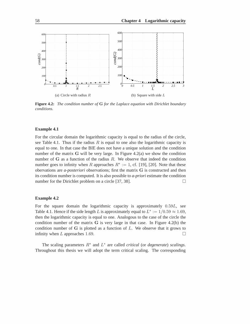
58 Chapter 4 Logarithmic capacity
0.5 1 1.5 2 2.50
100
200
300
400
500
600
R
con
d(G
)
(a) Circle with radiusR
0 0.5 1 1.5 2 2.5 30
100
200
300
400
500
600
L
con
d(G
)
(b) Square with sideL
Figure 4.2: The condition number ofG for the Laplace equation with Dirichlet boundaryconditions.
Example 4.1
For the circular domain the logarithmic capacity is equal tothe radius of the circle,see Table 4.1. Thus if the radiusR is equal to one also the logarithmic capacity isequal to one. In that case the BIE does not have a unique solution and the conditionnumber of the matrixG will be very large. In Figure 4.2(a) we show the conditionnumber ofG as a function of the radiusR. We observe that indeed the conditionnumber goes to infinity whenR approachesR∗ := 1, cf. [19], [20]. Note that theseobervations area-posterioriobservations; first the matrixG is constructed and thenits condition number is computed. It is also possible toa-priori estimate the conditionnumber for the Dirichlet problem on a circle [37, 38].
Example 4.2
For the square domain the logarithmic capacity is approximately 0.59L, seeTable 4.1. Hence if the side lengthL is approximately equal toL∗ := 1/0.59 ≈ 1.69,then the logarithmic capacity is equal to one. Analogous to the case of the circle thecondition number of the matrixG is very large in that case. In Figure 4.2(b) thecondition number ofG is plotted as a function ofL. We observe that it grows toinfinity whenL approaches1.69.
The scaling parametersR∗ andL∗ are calledcritical (or degenerate) scalings.Throughout this thesis we will adopt the term critical scaling. The corresponding

Section 4.6 Examples 59
0.5 1 1.5 210
−4
10−3
10−2
10−1
a
σ min.
σmin
(G)
σmin
(G1)
Figure 4.3: The smallest singular value of the matricesG (circles) andG1 (diamonds) forthe Laplace problem with mixed boundary conditions on an ellipsoidal domain.
domain is referred to as thecritical domain. A description for the boundary of acritical domain which frequently appears in literature isΓ-contour[56].
It is obvious that we cannot use the boundary element formulation if thelogarithmic capacity is equal to one. In Section 4.3 we suggested to search forsolutionsq of the Dirichlet BIE that also satisfy the requirement (4.15), i.e. havecontour integral equal to zero. Translating this requirement to the discrete problem,we have to search for solutionsq that also satisfyq1 + . . .+ qN = 0. Hence we haveto solve the rectangular system
G
H . . . H
︸ ︷︷ ︸
G1
q1...qN
=
f1...fN
0
. (4.39)
Here the additional condition is multiplied by a non-zero scalarH in order to obtain awell-balanced matrixG1. As we have a rectangular system, we require other solutiontechniques to solve the system, compared to the original system.
Example 4.3
To investigate the conditioning of the new system in (4.39),we compare the smallestsingular values ofG andG1. We illustrate this for an ellipsoidal domain with axisa anda/2. In Table 4.1 it is given that the logarithmic capacity of such an ellipseis equal to3a/4. Hence if we choosea equal to the critical valuea∗ = 4/3the logarithmic capacity is equal to one. In Figure 4.3 bothσmin(G) (circles)and σmin(G1) (diamonds) are plotted as a function of the scaling parameter a.
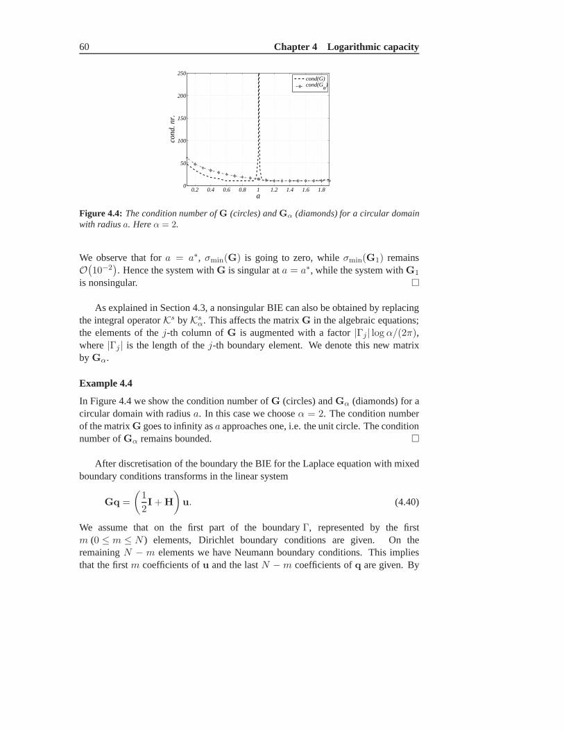
60 Chapter 4 Logarithmic capacity
0.2 0.4 0.6 0.8 1 1.2 1.4 1.6 1.80
50
100
150
200
250
a
con
d.
nr.
cond(G)cond(Gα)
Figure 4.4: The condition number ofG (circles) andGα (diamonds) for a circular domainwith radiusa. Hereα = 2.
We observe that fora = a∗, σmin(G) is going to zero, whileσmin(G1) remainsO
(10−2
). Hence the system withG is singular ata = a∗, while the system withG1
is nonsingular.
As explained in Section 4.3, a nonsingular BIE can also be obtained by replacingthe integral operatorKs byKs
α. This affects the matrixG in the algebraic equations;the elements of thej-th column ofG is augmented with a factor|Γj| log α/(2π),where|Γj | is the length of thej-th boundary element. We denote this new matrixby Gα.
Example 4.4
In Figure 4.4 we show the condition number ofG (circles) andGα (diamonds) for acircular domain with radiusa. In this case we chooseα = 2. The condition numberof the matrixG goes to infinity asa approaches one, i.e. the unit circle. The conditionnumber ofGα remains bounded.
After discretisation of the boundary the BIE for the Laplaceequation with mixedboundary conditions transforms in the linear system
Gq =
(1
2I + H
)
u. (4.40)
We assume that on the first part of the boundaryΓ, represented by the firstm (0 ≤ m ≤ N ) elements, Dirichlet boundary conditions are given. On theremainingN − m elements we have Neumann boundary conditions. This impliesthat the firstm coefficients ofu and the lastN −m coefficients ofq are given. By

Section 4.6 Examples 61
0.5 1 1.5 2 2.5 30
100
200
300
400
500
l
con
d. n
r.
cond(A)cond(G)
(a) Triangle
0.5 1 1.5 20
100
200
300
400
500
a
con
d. n
r.
cond(A)cond(G)
(b) Ellipse
Figure 4.5: The condition number of the matricesA (circles) and G (squares)corresponding to the Laplace equation with mixed boundary conditions and Dirichletboundary conditions respectively.
moving all unknown coefficients to the left-hand side and allknown coefficients tothe right-hand side in (4.40) we arrive at the standard form linear system
Ax = b. (4.41)
If the BIE is not uniquely solvable, then the linear system issingular, and thecondition number of the matrixA is very large. We illustrate this with two examples:a triangular domain and an ellipsoidal domain.
Example 4.5
The triangle is an isosceles right triangle with sides of length l. For such a trianglethe logarithmic capacity is given by
Cl(triangle) =33/4Γ2(1/4)
27/2π3/2l ≈ 0.476 l. (4.42)
This implies that the condition number will be large when thescaling parameterl isclose to the critical scalingl∗ := 1/0.476 ≈ 2.1. The ellipse has semi-axes of lengtha anda/2, which has logarithmic capacity equal to3a/4. Hence we may expect alarge condition number when the scaling parametera is close toa∗ := 4/3.
In Figure 4.5 we show the condition numbers for the matricesA andG. WechooseN = 32 and m = N/2, i.e. the number of elements with Dirichletconditions is equal to the number of elements with Neumann conditions. The circlesrepresent the condition number for the mixed problem, whilethe squares representthe condition number for the Dirichlet problem. We observe that the the critical
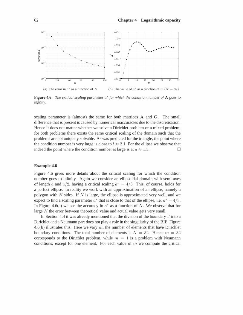
62 Chapter 4 Logarithmic capacity
0 20 40 60 80 10010
−4
10−3
10−2
10−1
N
err
or
in a
*
(a) The error ina∗ as a function ofN .
0 5 10 15 20 25 30 351.334
1.335
1.336
1.337
1.338
1.339
1.34
1.341
m
a*
(b) The value ofa∗ as a function ofm (N = 32).
Figure 4.6: The critical scaling parametera∗ for which the condition number ofA goes toinfinity.
scaling parameter is (almost) the same for both matricesA and G. The smalldifference that is present is caused by numerical inaccuracies due to the discretisation.Hence it does not matter whether we solve a Dirichlet problemor a mixed problem;for both problems there exists the same critical scaling of the domain such that theproblems are not uniquely solvable. As was predicted for thetriangle, the point wherethe condition number is very large is close tol ≈ 2.1. For the ellipse we observe thatindeed the point where the condition number is large is ata ≈ 1.3.
Example 4.6
Figure 4.6 gives more details about the critical scaling forwhich the conditionnumber goes to infinity. Again we consider an ellipsoidal domain with semi-axesof lengtha anda/2, having a critical scalinga∗ = 4/3. This, of course, holds fora perfect ellipse. In reality we work with an approximation of an ellipse, namely apolygon withN sides. IfN is large, the ellipse is approximated very well, and weexpect to find a scaling parametera∗ that is close to that of the ellipse, i.e.a∗ = 4/3.In Figure 4.6(a) we see the accuracy ina∗ as a function ofN . We observe that forlargeN the error between theoretical value and actual value gets very small.
In Section 4.4 it was already mentioned that the division of the boundaryΓ into aDirichlet and a Neumann part does not play a role in the singularity of the BIE. Figure4.6(b) illustrates this. Here we varym, the number of elements that have Dirichletboundary conditions. The total number of elements isN = 32. Hencem = 32corresponds to the Dirichlet problem, whilem = 1 is a problem with Neumannconditions, except for one element. For each value ofm we compute the critical

Section 4.6 Examples 63
scalinga∗. We see that there is little change in the value ofa∗ asm varies between1andN .
As the mixed problem is ill-posed when the logarithmic capacity is equal to one,we may add an extra condition like we did for the Dirichlet problem. Sinceu satisfiesthe Laplace equation on the interior of the domain we know that q must have a zerocontour integral. This leads to the following condition forthe solution vectorq of thelinear system in (4.40),
q1 + . . .+ qm = −γ := −(qm+1 + . . . + qN), (4.43)
since part of the vectorq is already prescribed by the boundary condition atΓ2. Likewe did for the Dirichlet case we formulate a new linear systemin which the extracondition is incorporated,
A
H . . .H 0 . . . 0
︸ ︷︷ ︸
A1
x1...xN
=
b1...bN
−Hγ
. (4.44)
Here the additional condition is multiplied by a non-zero scalarH to obtain a well-balanced system matrix.
Example 4.7
We compare the smallest singular valueσmin(A) of the original matrixA to thesmallest singular valueσmin(A1) of the new matrixA1 for the example of the ellipsewith semi-axesa anda/2. In Figure 4.7 we give the smallest singular values of thematricesA (circles) andA1 (diamonds) as a function of the scaling parametera.We observe that for the scalinga = a∗, σmin(A) drops to zero, whileσmin(A1)remainsO
(10−2
). Hence the system withA is singular ata = a∗ while the system
with A1 is nonsingular.
Another procedure to obtain a nonsingular BIE is to replace the integral operatorKs by Ks
α, see Section 4.4. This affects the matrixG as described before, and asA
inherits a block fromG, alsoA is affected. We denote the new matrix byAα.
Example 4.8
In Figure 4.8 we show the condition number ofA (circles) andAα (diamonds) fora circular domain with radiusR. In this case we choose the parameterα equal to

64 Chapter 4 Logarithmic capacity
0.5 1 1.5 210
−5
10−4
10−3
10−2
10−1
a
σ min.
σmin
(A)
σmin
(A1)
Figure 4.7: The condition number of the matricesA (circles) andA1 (diamonds) for theLaplace problem with mixed boundary conditions on an ellipsoidal domain.
0.2 0.4 0.6 0.8 1 1.2 1.4 1.6 1.80
50
100
150
200
250
300
350
400
R
con
d. n
r.
cond(A)cond(Aα)
Figure 4.8: The condition number ofA (circles) andAα (diamonds) for a circular domainwith radiusR. Hereα = 2.
two. As we have seen before, the condition number of the matrix A goes to infinityatR = R∗ := 1. The condition number ofAα remains bounded.
Another technique to ensure low condition numbers is by balancing the matrixelements ofG andH with a suitable scaling parameter of the domain [72].

Chapter 5
Two-dimensional Stokes flow
It was observed in Chapter 3 and 4 that the boundary integral equation (BIE) for theLaplace equation may become singular at certain critical two-dimensional domains.The main cause for this lies in the logarithmic kernel that appears in the boundaryintegral operator. In the boundary integral operator for the Stokes equations on a two-dimensional domain the logarithmic kernel also appears. Therefore we may expectsingular BIEs for the Stokes equations too. This is therefore the topic of this chapter.
The Stokes equations describe the flow of a viscous fluid. We briefly introducethe Stokes equations in differential form and the corresponding boundary integralformulation in dimensionless notation. For more details werefer to Chapter 6, inwhich the equations are derived in a three-dimensional setting. For the boundaryconditions we either choose Dirichlet or mixed boundary conditions. We will showthat for both cases there are critical sizes of the fluid domain for which the Stokesequations in boundary integral form are singular.
This chapter is an elaboration of earlier work of the author et al. [35] concerningcondition numbers of BEM-matrices that appear for the 2D Stokes equations.
5.1 Boundary integral equations for 2D Stokes flow
The Laplace equation and the Stokes equations have at least one thing in common: theLaplace operator appears in both equations. As we have seen in previous chapters,the Laplace equation may lead to a singular BIE for certain critical domains. Thequestion arises whether this is also the case for the Stokes equations: can thecorresponding BIEs become singular on certain critical domains?
In this chapter we study the BIEs following from the Stokes equations. Inparticular we focus on the eigenvalues of the integral operators. It is shown thatfor certain critical domains these integral operators admit zero eigenvalues. Hence,
65

66 Chapter 5 Two-dimensional Stokes flow
again we find that the BIEs become singular for a number of critical domains.For the Laplace equation it is possible toa-priori determine the critical domains.
For a number of simple domains, the logarithmic capacity canbe used to exactlycompute the critical size. For more involved domains the logarithmic capacity can beused to estimate the critical size of the domain. Unfortunately the critical domainsfor the Stokes equations do not coincide with the critical domains for the Laplaceequations. Hence we cannot use the logarithmic capacity toa-priori determine thecritical domains on which the BIEs for Stokes equations become singular. It is onlyby numerical experiments that we can distinguish the critical domains.
Let Ω be a two-dimensional simply-connected domainΩ with a smoothboundaryΓ. The Stokes equations for a viscous flow inΩ read
∇2v −∇p = 0,
∇.v = 0, (5.1)
wherev is the velocity field of the fluid andp its pressure. LetΓ be divided into apartΓ1 on which the velocityv is prescribed, and a partΓ2 on which the pressurepis prescribed,Γ = Γ1
⋃Γ2. Hence the Stokes equations are subject to the boundary
conditions
v = v, x ∈ Γ1,
p = p, x ∈ Γ2. (5.2)
Either Γ1 or Γ2 can be empty, leading to a purely Neumann or Dirichlet problemrespectively. The Stokes equations in differential form can be transformed to a set oftwo BIEs [65, 75, 76]
1
2vi(x) +
∫
Γqij(x,y)vj(y)dΓy
=
∫
Γuij(x,y)bj(y)dΓy, x ∈ Γ, i = 1, 2. (5.3)
Here a repeated index means summation over all possible values of that index. Thevector functionb is the normal stress at the fluid boundary,
b := σ(p,v)n, (5.4)
with n the outward unit normal at the boundary and the stress tensorσ defined by
σij(p,v) := −pδij +( ∂vi
∂xj+∂vj
∂xi
)
. (5.5)
Hence the boundary integral formulation involves two variables, the velocityv andthe normal stressb. In correspondence to (5.2), at each point of the boundary either

Section 5.2 Eigensystem of the single layer operatorG at a circle 67
v or b is prescribed,
v = v, x ∈ Γ1,b = −pn, x ∈ Γ2.
(5.6)
The kernelsuij andqij in the integral equations are defined as
qij(x,y) :=1
π
(xi − yi)(xj − yj)(xk − yk)nk
‖x− y‖4,
uij(x,y) :=1
4π
δij log1
‖x− y‖ +(xi − yi)(xj − yj)
‖x− y‖2
, (5.7)
for i, j = 1, 2. We introduce boundary integral operators,
(Gϕ)i(x) :=
∫
Γuij(x,y)ϕj(y)dΓy,
(Hψ)i(x) :=
∫
Γqij(x,y)ψj(y)dΓy, (5.8)
which enables us to write (5.3) as
(1
2I + H)v = Gb. (5.9)
The operatorsG andH are called thesingle and double layer operatorfor the Stokesequations. For the Dirichlet problem the velocityv at the boundary is given (Γ2 = ∅)and we would like to reconstruct the normal stressb at the boundary. To this end weneed to invert the operatorG. This can only be done when all eigenvalues ofG areunequal to zero. In this chapter we investigate under which conditionsG admits azero eigenvalue.
For the mixed problem the velocity atΓ1 is prescribed and the normal stress atΓ2 is prescribed. We would like to reconstruct the unknown velocity at Γ2 and theunknown normal stress atΓ1. After rearranging known and unknown terms (seeSection 5.4) we again need to invert a boundary integral operator. This can only bedone when all eigenvalues of the operator are unequal to zero. We will show that zeroeigenvalues occur under the same conditions as for the Dirichlet problem.
This chapter does not address the Stokes equations with Neumann conditions. Itis well known that the corresponding BIEs do not have a uniquesolution, due to theexistence of rigid body motions. The Completed Double LayerBEM [75] shows oneway to get around this problem.
5.2 Eigensystem of the single layer operatorG at a circle
For a circular domain it is possible to compute the eigenvalues of the single layeroperatorG analytically. These eigenvalues will show that for a circlewith a particular
68 Chapter 5 Two-dimensional Stokes flow
radius the BIE becomes singular. For general domains it is not possible to computethe eigenvalues ofG analytically. However the BIEs become also singular at certaindomains. This phenomenon for arbitrary domains is presented in the next section.In the current section we compute eigenfunctions and eigenvalues of the operatorGfor a circular boundaryΓ. Here we make use of the fact that the first term in thekerneluij is related to the fundamental solution for the Laplace operator in 2D. Thisresults in the following decomposition of the single layer operatorG for the Stokesequations,
(Gϕ)i(x) =1
2δij(Ksϕj)(x) +
1
4π
∫
Γ
(xi − yi)(xj − yj)
‖x− y‖2ϕj(y)dΓy. (5.10)
The operatorKs is the single layer operator for the Laplace equation. ForΓ a circlewith radiusR, the single-layer potentialKs admits the following eigensystem [38],
Ks cos(kt) =R
2kcos(kt),
Ks sin(kt) =R
2ksin(kt),
Ks1 = −R logR, (5.11)
with k ∈ N. We introduce the following polar coordinates,
x := R[cos t, sin t], y := R[cos s, sin s], 0 ≤ t, s < 2π. (5.12)
Then‖x− y‖2 = 2R2(1 − cos(t− s)) and we find
u11(t, s) =1
8π
− log[2R2(1 − cos(t− s))
]+
(cos t− cos s)2
1 − cos(t− s)
,
u12(t, s) =1
8π
(cos t− cos s)(sin t− sin s)
1 − cos(t− s),
u21(t, s) =1
8π
(sin t− sin s)(cos t− cos s)
1 − cos(t− s)= u12(t, s),
u22(t, s) =1
8π
− log[2R2(1 − cos(t− s))
]+
(sin t− sin s)2
1 − cos(t− s)
. (5.13)
Using the integral kernels in polar coordinates given in (5.13) it is straightforward tocompute the eigenvalues and eigenvectors of the operatorG. The results are given inTable 5.1.
We observe that the functionb(x) = n = [cos t, sin t]T , representing the unitoutward normal, is an eigenfunction with eigenvalue zero. This can be explained asfollows: when we apply a stress in the direction of the normalat each point of theboundary, each stress having the same magnitude, the net contribution will be equal

Section 5.2 Eigensystem of the single layer operatorG at a circle 69
eigenvalue eigenfunctions
0
[cos tsin t
]
R2
[− sin t
cos t
]
R4
[cos t
− sin t
]
,
[sin tcos t
]
R4k , (k = 2, 3, . . .)
[cos(kt)sin(kt)
]
,
[cos(kt)
− sin(kt)
]
,
[sin(kt)cos(kt)
]
,
[− sin(kt)
cos(kt)
]
−12R logR+ 1
4R
[10
]
,
[01
]
Table 5.1: Eigenvalues and eigenfunctions of the single layer operator G.
to zero. This phenomenon is not restricted to the circle, butapplies to any shape ofthe boundary, as will be proven in Section 5.3. Hence, when solving the BIE (5.9)with Dirichlet boundary conditions, one has to exclude the normal from the solutionspace.
For the caseR = R∗ := exp(1/2), we see that there is another zero eigenvalue,which has an eigenspace with dimension two. The eigenfunctions correspond to auniform stress distribution; at each point of the boundary an equal stress is appliedin the same direction. This particular stress distributionwill cause a translation ofthe body. The circular boundary withR = R∗ is called acritical boundaryand thecircle itself acritical domain. The radius or scaleR∗ is called thecritical scaleordegenerate scale. Equation (5.9) with Dirichlet conditions at the critical boundarycannot be solved as the operatorG admits a zero eigenvalue. The corresponding BIEis singular and does not have a unique solution.
The situation in which the BIE is not uniquely solvable for a circle with criticalscale also occurs for the Dirichlet Laplace equation in 2D [19, 20, 22, 24, 38]. It isshown that the single-layer operator for the unit circle admits a zero eigenvalue, andconsequently it cannot be inverted. Hence, the same phenomenon appears for boththe Laplace and Stokes equations. The critical scale however is not the same for theLaplace and Stokes equations.

70 Chapter 5 Two-dimensional Stokes flow
5.3 Invertibility of single layer operator on general domain
In this section we study the solvability of the BIE (5.9) withDirichlet conditionson a smooth closed boundaryΓ. We search for eigenfunctionsb of the boundaryintegral operatorG with zero eigenvalue, henceGb = 0. If such eigenfunctions exist,the boundary integral operatorG is not invertible and the integral equation (5.9) isnot uniquely solvable. First we show that at least one such eigenfunction with zeroeigenvalue exists.
Theorem 5.1 For any smooth boundaryΓ the outward unit normaln(x) is aneigenfunction of the boundary integral operatorG with eigenvalue zero.
Proof. Thei-th component ofGn equals
(Gn)i =
∫
Γuij(x,y)nj(y)dΓy
=1
4π
∫
Γ
[
δij log1
‖x− y‖ +(xi − yi)(xj − yj)
‖x− y‖2
]
nj(y)dΓy
=1
4π
∫
Ω
∂
∂xj
[
δij log1
‖x− y‖ +(xi − yi)(xj − yj)
‖x− y‖2
]
dΩy
= −∫
Ω
∂
∂xjui
jdΩy = −∫
Ω∇.uidΩ = 0. (5.14)
Here the vectorui is the velocity due to aStokeslet[65], i.e. the velocity field inducedby a point force in theei-direction. This velocity field satisfies the incompressibilitycondition∇.ui = 0.
In Section 5.2 we already saw that for a circular boundary thenormal vectornis an eigenfunction ofG with eigenvalue zero. The current theorem generalizesthis result to arbitrary smooth closed boundaries. In the sequel of this section weassume that the solutions of the Dirichlet problem (5.9) aresought in a functionspace that excludes the normal. Hence the eigenfunctionsb of G we are looking forare perpendicular ton.
We now show that for each boundaryΓ there exist (at most) two critical scalingsof the boundary such that the operatorG in the Dirichlet problem (5.9) is notinvertible. This phenomenon has been observed and proven [41] and we will partlypresent the analysis here. In analogy to Section 5.2 the scaling for which the operatorG is not invertible is called acritical scaling, and the corresponding boundary acritical boundary. The domain that is enclosed by the critical boundary is referred toas thecritical domain.

Section 5.3 Invertibility of single layer operator on general domain 71
Theorem 5.2 For all given functionsf and constant vectorsd the system ofequations
Gb+ c = f ,∫
Γ bdΓ = d,(5.15)
has a unique solution pair(b, c), whereb is a function andc a constant vector.
Sketch of proof. The main idea is to show that the operator that maps the pair(b, c) to the left-hand side of (5.15) is an isomorphism [41].
We proceed by introducing the two unit vectorse1 = [1, 0]T ande2 = [0, 1]T .Theorem 5.2 quarantees that two pairs(b1, c1) and(b2, c2) exist that are the uniquesolutions to the two systems
Gb1 + c1 = 0,∫
Γ b1dΓ = e1,
Gb2 + c2 = 0,∫
Γ b2dΓ = e2.
(5.16)
We define the matrixCΓ asCΓ := [c1|c2].
Theorem 5.3 If det(CΓ) = 0, then the operatorG is not invertible.
Proof. Suppose thatdet(CΓ) = 0, then the columnsc1 andc2 are dependent, sayc1 = αc2 for someα ∈ R, α 6= 0. In that case
0 =(Gb1 + c1
)− α
(Gb2 + c2
)
= G(b1 − αb2) + αc2 − αc2
= G(b1 − αb2). (5.17)
The functionb1 − αb2 cannot be equal to zero, since this requires∫
Γ(b1 − αb2)dΓto be equal to zero, while we have
∫
Γ(b1 − αb2)dΓ = e1 − αe2 6= 0. (5.18)
Sob1−αb2 is an eigenfunction ofG with zero eigenvalue. This eigenfunction cannotbe equal to the normaln, sincen also requires
∫
Γ ndΓ = 0.
Corollary 5.4 There are (at most) two critical scalings of the domainΓ for whichthe operatorG is not invertible.
Proof. We rescale the domainΓ by a factora, i.e. Γ → aΓ. With the definition ofthe operatorG it can be shown that
Gb→ Gab := − 1
4π
∫
Γa log a bdΓ + aGb. (5.19)

72 Chapter 5 Two-dimensional Stokes flow
Then the two systems in (5.16) change intoaGbj + cj − 1
4π
∫
Γ a log a bjdΓ = 0,
a∫
Γ bjdΓ = ej , j = 1, 2.
(5.20)
Definebja := abj for j = 1, 2, then we obtain
Gbj
a + cj − 14π
∫
Γ log a bjadΓ = 0,
∫
Γ bjadΓ = ej , j = 1, 2.
(5.21)
Substituting the second equation into the first equation, weget
Gbja + cj − 1
4π log a ej = 0,∫
Γ bjadΓ = ej, j = 1, 2.
(5.22)
These systems have the same form as the original systems in (5.16), except for thechangecj → cj − 1
4π log a ej for j = 1, 2. Define the new matrixCaΓ by
CaΓ := CΓ − 1
4πlog a I2, (5.23)
thenGa is not invertible whendet(CaΓ) = 0. Hence, when14π log a is an eigenvalue
of CΓ, the operatorGa is not invertible. This implies that, whenCΓ has two distincteigenvalues, there are two critical scalingsa for whichGa is not invertible. IfCΓ hasone eigenvalue with double multiplicity these critical scalings coincide.
The result of Corollary 5.4 shows that the BIEs for the Dirichlet Stokes equationsbecome singular for certain sizes of the domain. As a consequence, the equationsare not uniquely solvable. This solvability problem is an artifact of the boundaryintegral formulation; the Stokes equations in differential form always have a uniquesolution. In Chapter 3 and 4, and in literature [53, 56, 75, 85], a similar phenomenonis observed for the Laplace equation with Dirichlet conditions; in its differential formthe problem is well-posed, while the corresponding BIE is not solvable at criticalboundaries.
For the Laplace equation the critical scaling is related to the logarithmic capacityof the domain. By calculating or estimating the logarithmiccapacity one candetermine or estimate the critical domains, without computing BEM matrices andevaluating their condition numbers. It is thisa-priori information that allows us tomodify the standard BEM formulation such that the BIE becomeuniquely solvable(see Section 5.3).
For the Stokes equations, there does not exist an equivalentto the logarithmiccapacity. Hence we cannota-priori determine the critical domains. One way todetermine the critical domains is by computing the BEM-matrices and evaluating

Section 5.4 Invertibility of operator on general domain with mixed conditions73
their condition numbers. If the condition number jumps to infinity for a certaindomain, then this domain is a critical domain. Hence, this strategy requires thesolution of many BEM problems.
Another possibility to determine the critical domains is bysolving the systems in(5.16). This yields the matrixCΓ, and subsequently the matrixCaΓ. By calculatingthe eigenvalues of the latter matrix the critical scalings can be found. Again we haveto solve two non-standard BEM problems to compute the critical scalings.
REMARK : The BIEs for the Stokes flow in 2D are similar to the equationsfor plane elasticity. Hence the BIEs for the latter equations suffer from the samesolvability problems as the Stokes equations. A proof of this phenomenon for planeelasticity is found in literature [95] and is similar to the proof sketched above.
5.4 Invertibility of operator on general domain with mixedconditions
In the previous section we showed that the boundary integraloperatorG for theDirichlet Stokes equations is not invertible for all domains. In this section weshow that this phenomenon extends to the Stokes equations with mixed boundaryconditions.
The starting point is again the BIE for the Stokes equations,
1
2v + Hv = Gb, atΓ. (5.24)
Suppose that the boundaryΓ is split into two parts,Γ = Γ1⋃
Γ2. OnΓ1 we prescribethe velocityv1 while the normal stressb1 is unknown. OnΓ2 we prescribe the normalstressb2 while the velocityv2 is unknown. The boundary integral operatorsG andH are split accordingly,
[Gb]i =
∫
ΓuijbjdΓ =
∫
Γ1
uijb1jdΓ +
∫
Γ2
uijb2jdΓ =: [G1b1]i + [G2b2]i,
[Hv]i =
∫
ΓqijvjdΓ =
∫
Γ1
qijv1jdΓ +
∫
Γ2
qijv2j dΓ =: [H1v1]i + [H2v2]i.
(5.25)
With these notations the BIE is written in the following way,
1
2vk + H1v1 + H2v2 = G1b1 + G2b2, atΓk, k = 1, 2. (5.26)
We arrange the terms in such a way that all unknowns are at the left-hand side and all

74 Chapter 5 Two-dimensional Stokes flow
knowns are at the right-hand side,
H2v2 − G1b1 = G2b2 −H1v1 − 1
2v1, atΓ1,
1
2v2 + H2v2 − G1b1 = G2b2 −H1v1, atΓ2. (5.27)
Now we can define an operatorA that assigns to the pair(b1,v2) the two functionsat the left-hand side of (5.27),
[b1
v2
]
A→[
H2v2 − G1b1
12v
2 + H2v2 − G1b1
]
(5.28)
To study the invertibility of this operator we need to study the homogeneous versionof the equations in (5.27),
H2v2 − G1b1 = 0, atΓ1,1
2v2 + H2v2 − G1b1 = 0, atΓ2. (5.29)
Theorem 5.5 There are (at most) two scalings ofΓ such that the homogeneousequations (5.29) have a non-trivial solution, i.e.A is not invertible.
Proof. From the Dirichlet problem we know that there are (at most) two scalingsof Γ for whichG is not invertible. So there areaI andaII ∈ R and vector functionsqI andqII such that
Gqk = 0, atakΓ, k = I, II. (5.30)
The scalingsak and functionsqk may coincide but this does not affect the proof of thetheorem. Denote the nullspace of the operatorG by N(G). The normal vectorn isalways inN(G). If Γ is a critical boundary then alsoqI andqII are inN(G). AssumethatΓ is such a critical boundary. Letq ∈ N(G), that isq = α1qI +α2qII +α3n, forsomeα1, α2 andα3 in R, andGq = 0. Consider the homogeneous equations (5.29).We will show that there is a non-trivial pair(b1,v2) that satisfies these equations. Wechoosev2 = 0 andb1 = q1 + h1. Hereqi is the restriction ofq to Γi, i = 1, 2,andh1 is still unknown. Substituting these functions in the left-hand sides of thehomogeneous equations yields for both equations
−G1b1 = −G1q1 − G1h1 = G2q2 − G1h1, (5.31)
where we made use ofGq = G1q1 + G2q2 = 0. If we can find a functionh1 suchthatG1h1 = G2q2, then the left-hand sides of the homogeneous equations yield zeroand we have found a non-trivial solution. Our task is then to prove that a functionh1
exists such that
G1h1 = G2q2. (5.32)

Section 5.4 Invertibility of operator on general domain with mixed conditions75
A function b is in N(G)⊥ if it is perpendicular toq ∈ N(G)⊥. Hence, the innerproduct ofq andb should be equal to zero, i.e.
∫
Γqi(x)bi(x)dΓx = 0. (5.33)
First we note that the right-hand side of (5.32) is containedin N(G)⊥, since∫
Gqi[G2q2]idΓx =
∫
Γqi(x)
∫
Γ2
uij(x,y)q2j (y)dΓydΓx
=
∫
Γ2
q2j (y)
∫
Γuij(x,y)qi(x)dΓxdΓy
=
∫
Γ2
q2j (y)[Gq]jdΓy = 0. (5.34)
So we may generalize our task: prove that a solutionh1 of
G1h1 = φ (5.35)
exists, for anyφ ∈ N(G)⊥. If so, thenφ = G2q2 completes the proof. It is knownthat the operatorG is a Fredholm operator with index zero [29]. Hence the Fredholmalternative can be applied [70, p. 37]. This states that the homogeneous equationGh = 0 either has the trivial solution, or a set of non-trivial linearly independentsolutions. We are in the second situation, as the nullspace of G is non-empty and isspanned byn, qI andqII . The Fredholm alternative further states thatGh = φ issolvable if and only ifφ is perpendicular to the solutions ofG∗f = 0, whereG∗
denotes the adjoint operator ofG. However, the single layer operator for the Stokesequations is self-adjoint, soG∗ = G. Consequently the solvability condition saysthatφ has to be perpendicular to the solutions ofGh = 0. This is the case since wedefinedφ ∈ N(G)⊥. Consequently there exists anh with Gh = φ, for φ ∈ N(G)⊥.We split thish into two parts,
h =
h1, atΓ1,
h2, atΓ2.(5.36)
Recall that we search forh1 such thatG1h1 = φ. We addG2h2 to both sides of thisequation, obtaining
G1h1 + G2h2 = φ+ G2h2, (5.37)
or shorter
Gh = φ+ G2h2. (5.38)

76 Chapter 5 Two-dimensional Stokes flow
The right-hand side of this equation is inN(G)⊥, sinceφ ∈ N(G)⊥ and∫
Gqi[G2h2]idΓx =
∫
Γqi(x)
∫
Γ2
uij(x,y)h2j (y)dΓydΓx
=
∫
Γ2
h2j (y)
∫
Γuij(x,y)qi(x)dΓxdΓy
=
∫
Γ2
h2j (y)[Gq]jdΓy = 0, (5.39)
soG2h2 is also inN(G)⊥. Recall thatGh = φ+ G2h2 is solvable if the right-handside is inN(G)⊥, so there exists anh satisfying (5.38). Then we may constructh1
by simply restrictingh to Γ1, i.e.h1 = h|Γ1.
This result shows that also the BIE for the Stokes equations with mixed boundaryconditions may become singular. This happens for the same critical boundaries as forthe Stokes equations with Dirichlet boundary conditions. Hence the mixed probleminherits the singularities from the Dirichlet problem. Thedivision of the boundaryinto a Dirichlet and a Neumann part does not play a role in this.
Note that the Laplace equation exhibits the same behaviour.The boundaryintegral equation for the Laplace equation with mixed boundary conditions alsoinherits the solvability problems from the BIE for the Dirichlet case [39].
5.5 Numerical examples
To solve the BIEs (5.9), the boundaryΓ is discretised into a set ofN linear elements.At each element the velocityv and normal stressb are approximated linearly. In thisway the BIEs are transformed into a linear system of algebraic equations (for detailsabout the discretisation we refer to any BEM handbook [6, 10]). We introduce vectorsv andb of length2N containing the coefficients ofv andb at the nodal points. Thenthe system of equations can be written in short-hand notation as
(1
2I + H)v = Gb. (5.40)
HereG andH are the discrete counterparts of the single and double layeroperator.For the Dirichlet problem, the coefficients of the velocity vectorv are given, say
v = v, and we need to solve
Gb = f(v) := (1
2I + H)v (5.41)
to find the unknown coefficients of the normal stress vectorb.

Section 5.5 Numerical examples 77
If the boundary integral operatorG is not invertible then its discrete counterpart,the matrixG is ill-conditioned. To visualize this we compute the condition numberof G: if the condition number is infinitely large, then the matrixis not invertible. Asa consequence, the linear system (5.41) is singular and cannot be solved for arbitraryright-hand side vectorsf . If the condition number is bounded but very large, then stillthe problem (5.41) is difficult to solve numerically.
In the following examples we construct the matrixG for a certain boundaryΓand compute the condition number of this matrix. Then we rescale the boundaryΓby a factora, i.e. Γ → aΓ. Again we compute the condition number of the matrixG.We do this for several values of the scaling parametera. According to the theory inthe previous sections there are two critical scalings for which the integral operatorGis not invertible. For these two scalings also the matrixG is not invertible, or atleast very ill-conditioned. Hence we expect that the condition number ofG jumpsto infinity at these two scalings. The scaling for which such large condition numbersappear is again called acritical scalingand has ideally the same value as the criticalscaling defined for the BIE in the previous section. However,due to the discretisationof the equations, the critical scaling for the discrete problem may be slightly differentfrom the critical scaling for the BIE. In the limitN → ∞ these differences vanish.Analogously to the critical scaling, we define thecritical boundaryto be the boundaryfor which the condition number gets very large.
Example 5.1
In Figure 5.1 we show the condition number as a function of thescalea. We dothis for an ellipse with aspect ratio0.4 (to which we refer to as ellipse 1) and for anellipse with aspect ratio0.7 (to which we refer to as ellipse 2). We observe that forboth cases two critical scalings exist for which the condition number goes to infinity.Moreover, these critical scalings differ significantly forthe two ellipses. For ellipse 1we find critical scalings1.9 and2.9 approximately, while for ellipse 2 we find1.8and2.1. Hence the shape of the ellipse, i.e. its aspect ratio, greatly influences thevalues of the critical scalings.
Figure 5.2 visualises all ellipses for which the condition number ofG is verylarge, i.e. all critical ellipses with different aspect ratios. At the horizontal axis weput the lengtha of the horizontal semi-axis of the ellipse, at the vertical axis thelengthb of the vertical semi-axis of the ellipse. We compute the condition number ofG for several values ofa andb. We call the values ofa andb for which the conditionnumber goes to infinity thecritical sizesand the corresponding ellipse the criticalellipse. At thecritical sizeswe plot a dot in the(a, b)-plane of Figure 5.2. We seethat the critical sizes lie on two curved lines, which are symmetric around the linea = b. It can be concluded that for an ellipse with fixed aspect ratio d := a/b 6= 1,

78 Chapter 5 Two-dimensional Stokes flow
2 2.5 3
103
104
105
106
a
con
d(G
)
aspect ratio = 0.4aspect ratio = 0.7
Figure 5.1: Condition number ofG for an ellipsoidal domain with aspect ratios0.4 and0.7as a function of scaling parametera.
0 0.5 1 1.5 2 2.5 3 3.5 4 4.5 5 5.5 60
0.5
1
1.5
2
2.5
3
3.5
4
4.5
a
b
−a 0 a−b
0
b
Figure 5.2: The critical sizes of an ellipse for which the condition number ofG is very large.
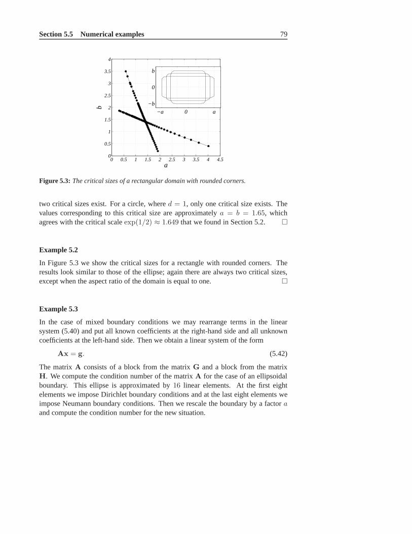
Section 5.5 Numerical examples 79
0 0.5 1 1.5 2 2.5 3 3.5 4 4.50
0.5
1
1.5
2
2.5
3
3.5
4
a
b
−a 0 a
−b
0
b
Figure 5.3: The critical sizes of a rectangular domain with rounded corners.
two critical sizes exist. For a circle, whered = 1, only one critical size exists. Thevalues corresponding to this critical size are approximately a = b = 1.65, whichagrees with the critical scaleexp(1/2) ≈ 1.649 that we found in Section 5.2.
Example 5.2
In Figure 5.3 we show the critical sizes for a rectangle with rounded corners. Theresults look similar to those of the ellipse; again there arealways two critical sizes,except when the aspect ratio of the domain is equal to one.
Example 5.3
In the case of mixed boundary conditions we may rearrange terms in the linearsystem (5.40) and put all known coefficients at the right-hand side and all unknowncoefficients at the left-hand side. Then we obtain a linear system of the form
Ax = g. (5.42)
The matrixA consists of a block from the matrixG and a block from the matrixH. We compute the condition number of the matrixA for the case of an ellipsoidalboundary. This ellipse is approximated by16 linear elements. At the first eightelements we impose Dirichlet boundary conditions and at thelast eight elements weimpose Neumann boundary conditions. Then we rescale the boundary by a factoraand compute the condition number for the new situation.

80 Chapter 5 Two-dimensional Stokes flow
1.5 2 2.5 310
1
102
103
104
105
106
107
a
con
d(A
)
aspect ratio = 0.4 .aspect ratio = 0.7 .
Figure 5.4: Condition number ofA for an ellipsoidal domain with aspect ratios0.4 and0.7with mixed boundary conditions, as a function of scalinga.
0 0.5 1 1.5 2 2.5 3 3.5 4 4.5 5 5.50
0.5
1
1.5
2
2.5
3
3.5
4
4.5
5
5.5
a
b
−a 0 a−b
0
b
Figure 5.5: The critical sizes of an ellipse with mixed boundary conditions for which thecondition number ofA is very large.
Figure 5.4 shows the condition number of the matrix for an ellipse with aspect ratio0.4 and an ellipse with aspect ratio0.7. We see that there exist two critical scalings foreach ellipse. For these critical ellipses the condition number ofA becomes infinitelylarge.
The critical sizes of the ellipse in the case of mixed conditions are close to the

Section 5.5 Numerical examples 81
0 0.5 1 1.5 2 2.5 3 3.5 40
0.5
1
1.5
2
2.5
3
3.5
4
a
b−a 0 a
−b
0
b
Figure 5.6: The critical sizes of rectangle with rounded corners with mixed boundaryconditions for which the condition number ofA is very large.
critical sizes for the case of Dirichlet conditions. In Figure 5.5 we show all criticalsizes of the ellipse for the case of mixed conditions. One canobserve that this plotresembles the plot in Figure 5.2 for Dirichlet conditions. This confirms the idea thatthe BIE for the mixed case inherits the solvability problem from the BIE for theDirichlet case. Note that the graph in Figure 5.6 is not symmetric anymore, as wasthe case for Dirichlet boundary conditions. This asymmetries are caused by the factthat the Dirichlet elements and Neumann elements are not distributed symmetricallyover the boundary.
Example 5.4
In Figure 5.6 we show the critical sizes of a rectangular domain with rounded cornerswith mixed boundary conditions. The results look similar tothose of rectangle withDirichlet conditions (Figure 5.3).
Example 5.5
We now turn our attention to a time-dependent problem. We study a viscous drop offluid of ellipsoidal shape that deforms to a circle due to surface tension. The evolutionof the boundary of the drop is governed by the Stokes equations and can be solvedusing the BEM [78, 93]. The velocityv of the boundary and the normal stressb atthe boundary are related by the BIE (5.9). The normal stressb is proportional to the

82 Chapter 5 Two-dimensional Stokes flow
Figure 5.7: An ellipse with aspect ratio0.5 deforming to a circle.
mean curvatureκ of the boundary,
b = −2γκn, (5.43)
with γ the surface tension andn the outward normal at the boundary.At time levelt = t1 we compute the velocityv at all discretisation nodesx. We
fix a time step∆t and update the boundary of the drop with an Euler forward step,
x→ x+ ∆tv(x), (5.44)
obtaining a new boundary. For this new boundary we again compute the velocity, andperform another Euler forward step. In this way we can study the shape evolution ofthe boundary. In Figure 5.7 we see the evolution of the ellipse to a circle. The initialshape is an ellipse with aspect ratio0.5 and the longest semi-axis has a length1.2. Wechoose40 points to discretise the boundary, the size of the time step is ∆t = 0.375and we compute10 time steps.
In the problem described above the normal stress is prescribed and the velocityhas to be reconstructed with equation (5.9). We can also formulate a problem inwhich we try to reconstruct the normal stress given the boundary velocity. It is thisproblem that we study in this example. To solve this problem we need to invert thematrix G at each time step. We know that there are certain critical boundaries forwhich the matrixG will not be invertible. In the problem of the deforming ellipse wego through a whole range of ellipses with different shapes, and we risk to encounterone or more of those critical boundaries.
In Figure 5.8 we show the condition number of the matrixG at each time stepfor a certain ellipse. An increase in the condition number indicates that the boundary

Section 5.5 Numerical examples 83
0 0.01 0.02 0.03 0.04 0.05 0.0610
2
104
106
108
1010
time
con
d(G
)
Figure 5.8: The condition number ofG at each time step without scaling.
0 0.01 0.02 0.03 0.04 0.05 0.06
104
106
108
time
con
d(G
)
Figure 5.9: The condition number ofG at each time step with temporary scaling when thedomain is close to a critical domain.
under consideration is close to a critical boundary. We see that there is one time levelin which such a critical boundary is reached. In this case we choose20 discretisationpoints, a time step size∆t = 0.002 and30 time steps.
There is a simple way to avoid a critical boundary. When the size of the boundarygets close to the critical boundary, we temporarily scale the domain. In Figure 5.9
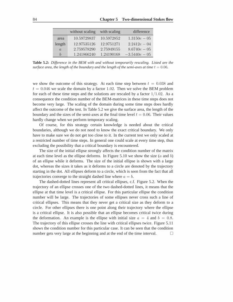
84 Chapter 5 Two-dimensional Stokes flow
without scaling with scaling difference
area 10.59729837 10.5972852 1.3150e − 05
length 12.97535126 12.9751271 2.2412e − 04a 2.759578290 2.75949155 8.6740e − 05b 1.241866240 1.24190168 −3.5440e − 05
Table 5.2: Difference in the BEM with and without temporarily rescaling. Listed are thesurface area, the length of the boundary and the length of thesemi-axes at timet = 0.06.
we show the outcome of this strategy. At each time step between t = 0.038 andt = 0.046 we scale the domain by a factor1.02. Then we solve the BEM problemfor each of these time steps and the solutions are rescaled bya factor1/1.02. As aconsequence the condition number of the BEM-matrices in these time steps does notbecome very large. The scaling of the domain during some timesteps does hardlyaffect the outcome of the test. In Table 5.2 we give the surface area, the length of theboundary and the sizes of the semi-axes at the final time levelt = 0.06. Their valueshardly change when we perform temporary scaling.
Of course, for this strategy certain knowledge is needed about the criticalboundaries, although we do not need to know the exact critical boundary. We onlyhave to make sure we do not get too close to it. In the current test we only scaled ata restricted number of time steps. In general one could scaleat every time step, thusexcluding the possibility that a critical boundary is encountered.
The size of the initial ellipse strongly affects the condition number of the matrixat each time level as the ellipse deforms. In Figure 5.10 we show the size (a andb)of an ellipse while it deforms. The size of the initial ellipse is shown with a largedot, whereas the sizes it takes as it deforms to a circle are denoted by the trajectorystarting in the dot. All ellipses deform to a circle, which isseen from the fact that alltrajectories converge to the straight dashed line wherea = b.
The dashed-dotted lines represent all critical ellipses, c.f. Figure 5.2. When thetrajectory of an ellipse crosses one of the two dashed-dotted lines, it means that theellipse at that time level is a critical ellipse. For this particular ellipse the conditionnumber will be large. The trajectories of some ellipses never cross such a line ofcritical ellipses. This means that they never get a criticalsize as they deform to acircle. For other ellipses there is one point along their trajectory where the ellipseis a critical ellipse. It is also possible that an ellipse becomes critical twice duringthe deformation. An example is the ellipse with initial sizea = 4 and b = 0.8.The trajectory of this ellipse crosses the line with critical ellipses twice. Figure 5.11shows the condition number for this particular case. It can be seen that the conditionnumber gets very large at the beginning and at the end of the time interval.

Section 5.5 Numerical examples 85
0 0.5 1 1.5 2 2.5 3 3.5 4 4.5 5 5.5 60
0.5
1
1.5
2
2.5
3
3.5
4
4.5
a
b
Figure 5.10: Each solid line represents the size of an ellipse as it deforms to a circle. Theinitial size, i.e. the lengthsa andb of the semi-axes, is denoted with a large dot. The dashed-dotted lines represent the critical sizes. The dashed line represents all circles.
0 1 2 3 4 5 610
2
104
106
108
time
con
d(G
)
Figure 5.11: The condition number for the ellipse with initial valuesa = 4 and b = 0.8.During the deformation to a circle this particular ellipse gets a critical size twice.

86 Chapter 5 Two-dimensional Stokes flow
p r e s s u r e
f l u i d
x = 1 x = 1 + d
dG 1
G 0
x
y
G 2 G 2
Figure 5.12: A viscous fluid is positioned into a mould. The boundary of thefluid consists oftwo semi-circles having radii1 and1 + d.
5.6 Blowing problem in 2D
It is shown that the Helmholtz boundary integral equation for domains with thin partscauses numerical instabilities, especially as the thickness of the thin part approacheszero; this phenomenon is calledthin-shape breakdown[32, 69]. In this section weinvestigate whether a similar phenomenon exists for the BIEs for the Stokes equationsin 2D. In particular we want to know how the BEM-matrices are affected by a part ofthe domain whose thickness approaches zero.
To this end we study a special application of the Stokes equations, a problem thatoccurs in the blowing of glass bottles, as explained in Chapter 6 . In this probleman amount of viscous fluid is positioned into a mould as depicted in Figure 5.12. Atthe topy = 0 (Γ2) the fluid is fixed, while it is free to move everywhere else. AttheboundaryΓ1 a pressurep1 is applied, which causes the fluid to move downwards andsideways, into the mould. In the current section we investigate the blowing problemfor an arbitrary viscous fluid. We do not address the time-dependent problem: for acertain initial shape we compute the velocity field of the fluid.
The flow of viscous fluids is described by the Stokes equations. The BEM cansolve these equations and yields the velocity field at the boundary of the fluid. Inthis section we investigate whether the BEM-matrices that appear when solving theblowing problem become singular. We assume that the fluid is rotationally symmetricsuch that we can investigate the flow in a 2D setting. The initial boundary of the fluid

Section 5.6 Blowing problem in 2D 87
consists of two concentric semi-circles separated by a distanced, as can be seen inFigure 5.12. The inner circle has radius1, so the outer circle has radius1 + d. Theidea is thatd will always be small compared to the radii of the circles, thus creatinga thin structure.
The boundary value problem that has to be solved for the blowing problem isgiven by (for more details we refer to Chapter 6)
∇2v −∇p = 0, atΩ,
∇.v = 0, atΩ,
σn = 0, atΓ0,
σn = −p1n, atΓ1,
v = 0, atΓ2. (5.45)
Hence we prescribe the normal stress at the part of the boundary where the pressureis applied. At the other part of the free boundary we prescribe zero normal stress.The BEM transforms the boundary value problem into a linear system,
(1
2I + H)v = Gb, (5.46)
wherev andb are vectors with the coefficients of the velocity and the normal stressat each of theN nodes along the boundary. In this example we use linear elements;hence the velocity and normal stress vary linearly over eachelement. As the twoboundary partsΓ2 are very small, each part is modelled by one element only. Sincethe boundary of the domain mainly consists of two parts, i.e.the inner and the outersemi-circle, the matrixG can be written as a block matrix,
G =
[
G1 G2
G3 G4
]
. (5.47)
The block matrixG1 corresponds with integration over the inner semi-circleΓ1 whileall collocation nodes are atΓ1. Similarly G4 is related solely to the outer circleΓ0.Hence to compute these blocks we do not require any information from the oppositeboundary part. The block matricesG2 andG3 correspond to integration over onesemi-circle while the collocation nodes are at the oppositesemi-circle. Let us assumethat the number of boundary elementsN is an even number.If the unknowns in the vectorb are ordered as
b = [b1x, . . . , bN/2x , b1y, . . . , b
N/2y , bNx , . . . , b
N/2+1x , bNy , . . . , b
N/2+1y ]T , (5.48)

88 Chapter 5 Two-dimensional Stokes flow
d ‖G − G‖∞ d ‖G − G‖∞0.1 3.26 · 10−2 0.0025 1.72 · 10−3
0.05 2.06 · 10−2 0.001 7.57 · 10−4
0.025 1.23 · 10−2 0.0005 3.90 · 10−4
0.01 5.78 · 10−3 0.00025 1.99 · 10−4
0.005 3.18 · 10−3 0.0001 9.87 · 10−5
Table 5.3: The matrixG approaches the matrixG as the thicknessd goes to zero.
and the equations in the BEM are ordered in the following way,
equation atx1... in x-directionequation atxN/2
equation atx1... in y-directionequation atxN/2
equation atxN... in x-directionequation atxN/2+1
equation atxN... in y-directionequation atxN/2+1
, (5.49)
it can be shown that the matrixG approaches the singular matrixG in the limit d ↓ 0,
limd↓0
G = G :=
[G1 G1
G1 G1
]
. (5.50)
Table 5.3 shows the max-norm ofG − G for decreasing values ofd. We see that asd ↓ 0 indeedG → G. Thus the matrixG can be seen as a perturbation of the matrixG around the pointd = 0. Table 5.3 suggests that the difference betweenG andG
depends linearly ond.It is straightforward to see that any vectorx of the formx = [x1 −x1]
T , x1 ∈ RN ,
is an eigenvector ofG with eigenvalue0. Hence the eigenvalue0 has an eigenspacewith dimension (at least)N , and is spanned by
[1, 0, . . . , 0,−1, 0, . . . , 0]T , . . . , [0, . . . , 0, 1, 0, . . . , 0,−1]T
. (5.51)

Section 5.6 Blowing problem in 2D 89
m ‖G −GS‖∞ m ‖G − GS‖∞4 2.0 · 10−3 20 5.8 · 10−5
8 5.2 · 10−4 24 2.6 · 10−5
12 2.1 · 10−4 28 2.7 · 10−5
16 1.1 · 10−4 32 1.7 · 10−5
Table 5.4: The difference between the matrixG, computed with the help of a Gauss-Legendrescheme withm knots, and the matrixGS , computed with the help of an adaptive Simpsonscheme.
Consider the matrixG as a function ofd, G = G(d), and introduce a functionF : R
2N × R → R2N by
F (x, d) := G(d)x. (5.52)
If G(d) is computed exactly, there existN roots of the equationF = 0, namely(x∗, d∗), wherex∗ = [x1 −x1]
T , x1 ∈ RN , andd∗ = 0. However in realityG
cannot be computed exactly since we make use of numerical integration schemes toapproximate integrals, so in fact we deal with a matrixG + E, with ‖E‖ small. Ifthe numerical integration is performed very accurately, the matrixE approaches thezero matrix. For the true matrixG + E we findM ≤ N of roots of the equationF = 0, namely(x∗, d∗), wherex∗ ≈ [x1 − x1]
T , x1 ∈ RN , andd∗ small, but not
necessarily0.The numerical integration error that is made by the Gauss-Legendre quadrature
scheme that we use here is particularly large for the blowingproblem that we study.To illustrate this we first compute the BEM-matrixG by using an adaptive Simpsonscheme with accuracy10−16. Adaptive schemes put more effort in approximating theintegrals near singularities. These schemes keep increasing the number of knots nearsingularities, until the required accuracy is obtained. The Gauss-Legendre schemetreats each subinterval of the integration path equally, and does not verify whether acertain accuracy is obtained. Therefore the adaptive Simpson scheme approximatesintegrals with a logarithmic singularity much more accurate than the Gauss-Legendrescheme. We denote the matrix whose integrals are approximated with an adaptiveSimpson scheme byGS and compare it to the matricesG that are computed byusing a Gauss- Legendre scheme withm knots. In Table 5.4 we show the max-normof G−GS . We see that the matricesG approachGS very slowly. Even with as muchasm = 32 knots the difference betweenG andGS is still 10−5. Hence the Gauss-Legendre scheme is much less accurate than the adaptive Simpson scheme. Thecause of this large error lies in the fact that the two semi-circles of the boundary are

90 Chapter 5 Two-dimensional Stokes flow
0.005 0.01 0.015 0.02 0.025
104
106
108
1010
thickness d
con
d(G
)
(a) N = 18
0.005 0.01 0.015 0.02 0.025
104
106
108
1010
thickness d
con
d(G
)
(b) N = 20
0.005 0.01 0.015 0.02 0.025
104
106
108
1010
thickness d
con
d(G
)
(c) N = 22
Figure 5.13: The condition number of the BEM-matrixG as a function of the thicknessd ofthe geometry.
Section 5.6 Blowing problem in 2D 91
separated by a small distance. In the computations of the BEM-matrix G, integralsthat involve the termlog ‖x − y‖ have to be evaluated, wherex is a point at onesemi-circle andy a point at the opposite semi-circle. Hence whend approaches zero,the distance‖x− y‖ betweenx andy becomes very small, and a nearly logarithmicsingularity appears in the integrals. The Gauss-Legendre scheme cannot approximatesuch integrals accurately enough [49, 84].
As a consequence, the matrixG is not computed accurately, and the equationF = 0 has a number of roots(x∗, d∗) in which thed∗ are unequal to zero. Toillustrate this we compute the BEM-matrixG for several values ofd and computeits condition number. In Figure 5.13(a) we show the condition number ofG as afunction ofd. For this example the boundary of the fluid is discretised withN = 18boundary elements and the Gauss-Legendre scheme usesm = 6 knots. We observethat for 6 values ofd the condition number jumps to infinity. These values ofdcorrespond to the roots ofF = 0.
If we increase the number of boundary elementsN and compute the matrixelements ofG exactly, the number of roots ofF = 0 also increases, as there areN such roots. IfG is not computed exactly, as is the case with the Gauss-Legendrescheme, we may also expect to find more roots ofF = 0. Figure 5.13(b) andFigure 5.13(c) confirm this idea. For Figure 5.13(b) we choose N = 20 boundaryelements and for Figure 5.13(c) we chooseN = 22 boundary elements. ForN = 20we observe8 values ofd for which the condition number jumps to infinity, and forN = 22 even10 of such values.
If we improve the accuracy of the numerical integration, we expect to approachthe exact matrixG better. As a consequence the roots ofF = 0 should alsoapproach the roots of the exact equation better. Hence the values ofd∗ should goto 0 if we improve on the numerical integration. Figure 5.14 confirms this idea. ThematricesG whose condition numbers are shown in Figure 5.14(a) are computed witha Gauss-Legendre scheme withm = 6 knots. For the matrices in Figure 5.14(b) andFigure 5.14(c) we usem = 7 andm = 8 knots respectively. Indeed we observe thatthe values ofd for which the condition number jumps to infinity approach zero asmincreases.
As we already noted before, the Gauss-Legendre schemes are not the mostappropriate numerical integration schemes for this particular blowing problem.Adaptive schemes are better equipped for the blowing problem. In the next examplewe compute the BEM-matrixG for several values ofd using an adaptive Simpsonscheme with accuracy10−6. With this accuracy the integrals inG are approximatedaccurately enough compared to the Gauss-Legendre scheme, whose accuracy is only10−5 for m = 32. The condition number ofG is plotted in Figure 5.15. We see that,except ford ↓ 0, there is no other value ofd for which the condition number ofGgoes to infinity. The large condition number ford ↓ 0 is expected, asG approaches
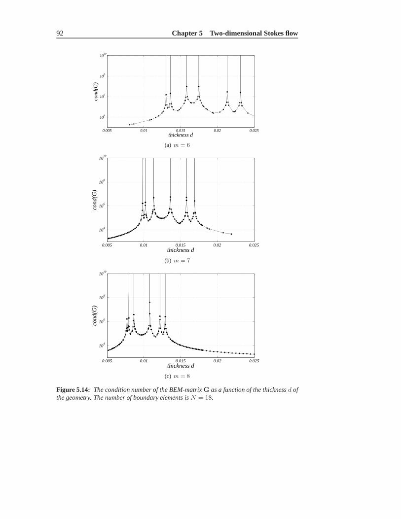
92 Chapter 5 Two-dimensional Stokes flow
0.005 0.01 0.015 0.02 0.025
104
106
108
1010
thickness d
con
d(G
)
(a) m = 6
0.005 0.01 0.015 0.02 0.025
104
106
108
1010
thickness d
con
d(G
)
(b) m = 7
0.005 0.01 0.015 0.02 0.025
104
106
108
1010
thickness d
con
d(G
)
(c) m = 8
Figure 5.14: The condition number of the BEM-matrixG as a function of the thicknessd ofthe geometry. The number of boundary elements isN = 18.

Section 5.6 Blowing problem in 2D 93
0 0.005 0.01 0.015 0.02 0.025
104
106
108
1010
thickness d
con
d(G
)
Figure 5.15: The condition number of the BEM-matrixG as a function of thicknessd.The number of boundary elements isN = 18. Numerical integration is performed withan adaptive Simpson scheme with accuracy10−6.
the singular matrixG very well in these cases.The blowing problem covered in this section shows that the numerical integration
needs special attention in the case of thin domains, i.e. twoboundary parts of thedomain are separated by a small distance only. For such domains, in particular forthe thin parts of such domains, the Gauss-Legendre quadrature scheme performspoorly when approximating the integrals that appear in the BEM-matrices. As aconsequence, for some values ofd the condition number ofG becomes infinitelylarge.

Chapter 6
Three-dimensional Stokes flow
In this chapter and the subsequent chapter we extend our research on the Stokesequations to three dimensions. We develop a mathematical model for a particularapplication: the blowing problem in 3D. We show that the BEM is a suitablenumerical method to solve such problems. These chapters arean elaboration ofearlier work of the author et al. [36, 40] concerning the numerical modelling ofthe blowing phase in the production of glass containers.
6.1 Simulating the blowing of glass containers with theBEM
In 3D the Stokes boundary integral equations cannot become singular at specific sizesor shapes of the domain, contrary to the Stokes boundary integral equations in 2D.The reason for this is the absence of a logarithmic term in thefundamental solutionfor the 3D Stokes equations. It is this logarithmic term thatis the essence of theexistence of critical domains in 2D. Hence we can safely construct a 3D BEM modelfor the class of blowing problems. In the blowing problem a viscous fluid is blown toa desired shape. We want to see whether the BEM is an appropriate numerical methodto solve this blowing problem. As a special application we consider the blowing ofglass containers.
The industrial production of glass containers like bottlesand jars consistsof several phases. First glass is moulten in a furnace where the glass reachestemperatures between1200 and 1600 C. The molten glass is then cut intogobs,which are transported to a forming machine.
The gob falls into a mould, and a plunger is pushed into the mould, shaping theglass to an intermediate form called theparison. This phase of the production process
94

Section 6.1 Simulating the blowing of glass containers withthe BEM 95
(a) Pressing phase (b) Blowing phase
Figure 6.1: The production of glass containers consists of a pressing phase and a blowingphase.
is called thepressing phase(Figure 6.1(a)). The parison is put into a second mould inwhich it is allowed to creep in vertical direction (sagging) due to gravity for a shortperiod of time. Then the parison is blown to its final shape by an inflow of pressurizedair. This phase of the production process is called theblowing phase(Figure 6.1(b)).
For the glass industry it is important to optimize each phaseof the productionprocess. One can think of optimizing the shape of the parison, the speed of theplunger, the sagging time, the pressure of the air during theblowing phase, etc [68].Experiments to tune these parameters are cumbersome, costly and time consuming.Therefore computer simulation of the various production phases can offer usefulinformation to optimize the production.
In this thesis we study the flow of the glass during the blowingphase. We assumethat the shape of the parison and the shape of the mould are given, and also thepressure of the inflowing air is prescribed. Given these settings the BEM computesthe velocity at the boundary of the glass by solving the Stokes equations. Then weperform a time integration step to obtain the shape of the glass at the next time level.For this new shape we again compute the velocity at the boundary and perform a newtime integration step. This iterative procedure enables usto study the shape evolutionof the glass during the blowing phase. The computations are performed in threedimensions. This allows studying bottles and jars that are not rotationally symmetric,for instance due to small imperfections in the initial parison.
Numerical modelling of the production process of glass bottles and jars has beenthe topic of several papers. Mostly finite element methods are used to simulate theglass flow [12, 13], sometimes using a level set method to track the position of the

96 Chapter 6 Three-dimensional Stokes flow
glass boundary [45]. In many cases rotationally symmetric parisons are modelled andcomputations are limited to two dimensions. To the author’sknowledge our work isthe first to address the blowing problem in three dimensions using the BEM.
During the blowing phase the temperature of the glass changes due to heatexchange with the mould. The viscosity of the glass depends on the temperaturein an essentially non-linear fashion. As the viscosity appears in the Stokes equations,the heat and flow problem are coupled. However we show that during the blowingphase we may consider a homogeneous temperature. Consequently also the viscositybecomes homogeneous and the heat and flow problem can be addressed separately.In the papers mentioned above the heat problem is studied intensively. In this thesiswe therefore focus on the flow problem.
In Figure 6.2 we schematically depict the glass and the mould. We assume that atthe top (S2) the glass touches the mould and cannot move. At the other parts wherethe glass touches the mould (S3) it is allowed to slip along the mould. At the inletof the mould (S1) pressurized air flows in, while at the bottom of the mould (S0)standard pressure is maintained.
Special attention has to be paid to the contact problem between the glass and themould. Most papers assume a no-slip condition at the mould surface, i.e. glass cannotslip along the surface. In practice this is not the case. Sometimes the mould is evencovered with a lubricating substance to improve the slip of the glass. Therefore wechoose to work with a partial-slip boundary condition instead of a no-slip boundarycondition.
The procedure described above results in a simulation tool that can be used tostudy the blowing phase for glass products. We have tested the simulation tool onseveral bottles and jars. The results of the tests are promising and may contribute toa better understanding of the production of bottles and jars.
6.2 Mathematical model
In this section we derive the mathematical model that describes the flow of aNewtonian fluid with high viscosity in three dimensions. Letthe fluid domain bedenoted byΩ, bounded by a closed surfaceS. The velocity and pressure of the fluidare denoted byv andp respectively. Furthermore the fluid is characterized by thedynamic viscosityη, a surface tensionγ and a typical length scaleL. In general theviscosityη depends on the temperature of the glass. As the temperature may be spacedependent, also the viscosity may be space dependent. However, later on we showthat for the blowing problem the glass has a uniform temperature distribution, andhenceforth the viscosity is uniform also.
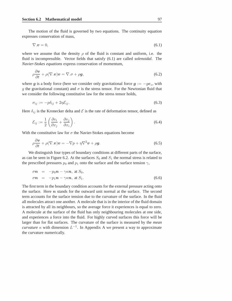
Section 6.2 Mathematical model 97
The motion of the fluid is governed by two equations. The continuity equationexpresses conservation of mass,
∇.v = 0, (6.1)
where we assume that the densityρ of the fluid is constant and uniform, i.e. thefluid is incompressible. Vector fields that satisfy (6.1) arecalled solenoidal. TheNavier-Stokes equationsexpress conservation of momentum,
ρ∂v
∂t+ ρ(∇.v)v = ∇.σ + ρg, (6.2)
whereg is a body force (here we consider only gravitational forceg := −gez, withg the gravitational constant) andσ is the stress tensor. For the Newtonian fluid thatwe consider the following constitutive law for the stress tensor holds,
σij := −pδij + 2ηEij . (6.3)
Hereδij is the Kronecker delta andE is the rate of deformation tensor, defined as
Eij :=1
2
(∂vi
∂xj+∂vj
∂xi
)
. (6.4)
With the constitutive law forσ the Navier-Stokes equations become
ρ∂v
∂t+ ρ(∇.v)v = −∇p+ η∇2v + ρg. (6.5)
We distinguish four types of boundary conditions at different parts of the surface,as can be seen in Figure 6.2. At the surfacesS0 andS1 the normal stress is related tothe prescribed pressuresp0 andp1 onto the surface and the surface tensionγ,
σn = −p0n− γκn, atS0,
σn = −p1n− γκn, atS1. (6.6)
The first term in the boundary condition accounts for the external pressure acting ontothe surface. Heren stands for the outward unit normal at the surface. The secondterm accounts for the surface tension due to the curvature ofthe surface. In the fluidall molecules attract one another. A molecule that is in the interior of the fluid domainis attracted by all its neighbours, so the average force it experiences is equal to zero.A molecule at the surface of the fluid has only neighbouring molecules at one side,and experiences a force into the fluid. For highly curved surfaces this force will belarger than for flat surfaces. The curvature of the surface ismeasured by themeancurvatureκ with dimensionL−1. In Appendix A we present a way to approximatethe curvature numerically.

98 Chapter 6 Three-dimensional Stokes flow
S 0
S 1
S 3
S 2
W
Figure 6.2: Cross-sectional view of the set-up of the blowing problem. The glass is positionedin a mould. The surface of the glass is divided into four parts.
At the surfaceS2 we assume that the fluid is in contact with the mould. The fluidis not allowed to slip and hence we set the velocity equal to zero,
v = 0, atS2. (6.7)
At the surfaceS3 the fluid is in contact with the mould, but is allowed to slip along thewall of the mould. This means that the velocity component in the normal direction tothe wall is equal to zero, i.e. the fluid cannot penetrate the wall,
v.n = 0, atS3. (6.8)
The velocity components in the tangential directions may not be zero. Navier’s sliplaw states that the tangential component of the velocity is related to the normal stressby [57, 67],
(σn+ βmv).t = 0, atS3. (6.9)
Heret is a vector in the tangential direction at the wall andβm is a friction parameter.If βm → 0 there is no friction between fluid and wall. Ifβm → ∞ the frictionbetween fluid and wall is very large and the fluid cannot flow along the wall.Condition (6.8) together with (6.9) yields the no-slip condition (6.7) whenβm = ∞.
We introduce a dimensionless pressurep′, velocityv′ and body forceg′ by
p′ :=p− p0
p1 − p0, v′ :=
v
vc:=
ηv
(p1 − p0)L, g′ := −ez. (6.10)

Section 6.2 Mathematical model 99
We also define a characteristic time scaletc := L/vc. Using these characteristicvariables and usingL as a characteristic length, we rewrite the Navier-Stokesequations in dimensionless form as
Re
(∂v′
∂t′+ (∇′.v′)v′
)
= −∇′p′ + ∇′2v′ +ReFrg′. (6.11)
Here the differential operator∇′ denotes differentiation with respect to thedimensionless spatial coordinates. The dimensionless numbers Re and Fr are theReynolds numberand theFroude numberrespectively, defined as
Re :=ρLvc
η,
Fr :=v2c
gL. (6.12)
For the type of fluids that we consider here, the Reynolds number is about10−3
or smaller. For instance, for glass the Reynolds number can be computed with thevalues of the material properties and process parameters inTable 6.1, and we findRe= 2.5 · 10−4. This implies that the convective term at the left-hand sideof (6.11)can be neglected. This reduces the Navier-Stokes equationsto theStokes equationswith body force term,
∇′2v′ −∇′p′ + αg′ = 0, (6.13)
whereα := Re/Fr. Together with the dimensionless form of (6.1)
∇′.v′ = 0, (6.14)
we obtain a system of four equations that describe the flow of the fluid. It can beverified that the dimensionless stress tensorσ′ is given by
σ′ := − p0
p1 − p0I +
1
p1 − p0σ. (6.15)
We also introduce a dimensionless curvatureκ′ by κ′ := Lκ. Substitution ofσ′ andκ′ into the boundary conditions atS0 andS1 yields
σ′n = −βκ′n, atS0,
σ′n = −(1 + βκ′)n, atS1, (6.16)
where the dimensionless numberβ is defined as
β :=γ
(p1 − p0)L. (6.17)
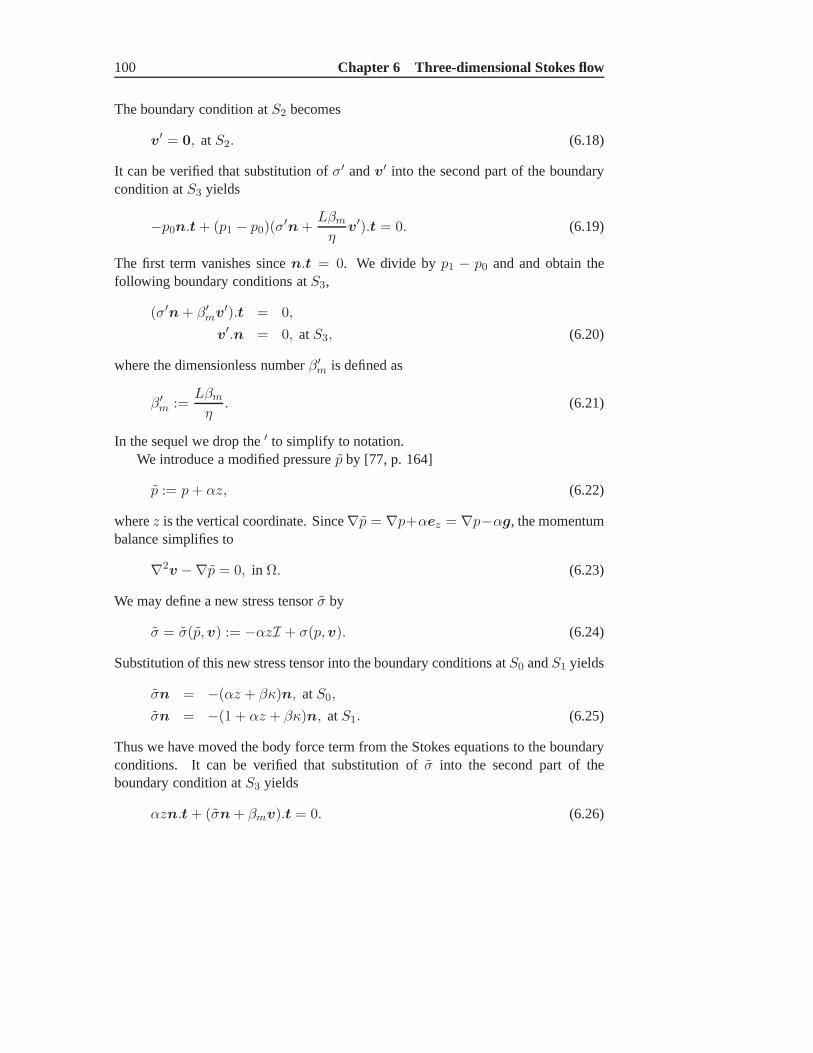
100 Chapter 6 Three-dimensional Stokes flow
The boundary condition atS2 becomes
v′ = 0, atS2. (6.18)
It can be verified that substitution ofσ′ andv′ into the second part of the boundarycondition atS3 yields
−p0n.t+ (p1 − p0)(σ′n+
Lβm
ηv′).t = 0. (6.19)
The first term vanishes sincen.t = 0. We divide byp1 − p0 and and obtain thefollowing boundary conditions atS3,
(σ′n+ β′mv′).t = 0,
v′.n = 0, atS3, (6.20)
where the dimensionless numberβ′m is defined as
β′m :=Lβm
η. (6.21)
In the sequel we drop the′ to simplify to notation.We introduce a modified pressurep by [77, p. 164]
p := p+ αz, (6.22)
wherez is the vertical coordinate. Since∇p = ∇p+αez = ∇p−αg, the momentumbalance simplifies to
∇2v −∇p = 0, in Ω. (6.23)
We may define a new stress tensorσ by
σ = σ(p,v) := −αzI + σ(p,v). (6.24)
Substitution of this new stress tensor into the boundary conditions atS0 andS1 yields
σn = −(αz + βκ)n, atS0,
σn = −(1 + αz + βκ)n, atS1. (6.25)
Thus we have moved the body force term from the Stokes equations to the boundaryconditions. It can be verified that substitution ofσ into the second part of theboundary condition atS3 yields
αzn.t+ (σn+ βmv).t = 0. (6.26)

Section 6.2 Mathematical model 101
The first term vanishes sincen.t = 0 and we obtain the following conditions atS3,
(σn+ βmv).t = 0,
v.n = 0, atS3, (6.27)
To summarize, the equations and boundary conditions in dimensionless form aregiven by
∇2v −∇p = 0, in Ω,
∇.v = 0, in Ω,
σn = −(αz + βκ)n, atS0,
σn = −(1 + αz + βκ)n, atS1,
v = 0, atS2,
(σn+ βmv).t = 0, atS3,
v.n = 0, atS3. (6.28)
In the sequal we will omit the.This thesis does not aim addressing the heat change in the glass and the heat
exchange between glass, air and mould. However, the temperature does enter theStokes equations via the viscosity of the glass. In general the viscosityη depends onthe temperature of the glass. Often in glass problems this dependence is modelledwith theVogel-Fulcher-Tamman relation[7], which is given by
η = η0 exp
(B
T − TV F
)
. (6.29)
HereT is the temperature of the glass andη0, B andTV F are the so-calledLakatoscoefficients.
We show that for the blowing problem it is not necessary to include thetemperature dependence of the viscosity into our model. To see this consider theenergy equation (still in dimension-full notation)
ρcp∂T
∂t+ v.∇T = kc∇2T + ∇ (kr(T )∇T )
+ η((∇v+ ∇vT ) : ∇v
). (6.30)
The three terms on the right-hand side of this equation represent the conduction,the radiation and the viscous dissipation respectively. The parameterscp, kc andkr
are the specific heat, the conductivity and the Rosseland parameter respectively. Weintroduce a dimensionless temperatureT ′ byT = Tm +∆TT ′, with ∆T = Tg−Tm,Tg being the initial temperature of the glass, andTm being the temperature of the

102 Chapter 6 Three-dimensional Stokes flow
parameter value dimensionL 0.01 mvc 0.01 m s−1
ρ 2500 kg m−3
η 1000 kg m−1s−1
cp 1350 J kg−1K−1
kc 1.5 W m−1K−1
Tg 1100 CTm 600 Cp0 1.00 · 105 kg m−1s−2
p1 1.38 · 105 kg m−1s−2
γ 0.3 kg s−2
Table 6.1: Material properties and process parameters for the glass blowing problem.
mould. The dimensionless form of the heat equation reads (weimmediately omitthe ′ )
∂T
∂t+ v.∇T =
1
Pe∇2T + ∇
(kr(T )
kc
1
Pe∇T
)
+EcRe
((∇v + ∇vT ) : ∇v
). (6.31)
Here thePeclet numberand theEckert numberare defined as
Pe:=ρcpvcL
kc, Ec :=
v2c
cp∆T. (6.32)
Typical values of the parameters involved (see Table 6.1) yield 1/Pe ≈ 10−3 andEc/Re ≈ 10−7. Hence the terms on the right-hand side can be neglected and theenergy equation reduces to
∂T
∂t+ v.∇T = 0. (6.33)
This implies that the temperature remains constant along streamlines. If we assumethat the initial temperature of the glass is uniform in spaceand the mould has auniform temperature too, it follows that the glass is isothermal. As a consequence,also the viscosity can be taken uniform. This shows that the Stokes equations and theheat equation are decoupled and can be solved separately. Inthis thesis, however, weare only interested in the flow problem.

Section 6.3 Boundary integral equations 103
6.3 Boundary integral equations
In this section the mathematical model summarized in (6.28)is transformed into aset of boundary integral equations [65]. We introduce a vector fielduk(x,y) and ascalar functionqk(x,y) that satisfy the following Stokes equations,
∇2xu
k(x,y) −∇xqk(x,y) = δ(x − y)ek,
∇x.u(x,y) = 0. (6.34)
The vectorek is a unit vector directed along thek − th coordinate axis,k = 1, 2, 3.The subscriptx means that differentiation is performed with respect to thespatialcoordinatex. The pointy is an arbitrary point inR3. Physically the equations (6.34)describe the velocity and pressure due to a unit point sourcein the ek-directionlocated at the pointy. Using the requirements
ukj (x,y) = O
(1
‖x− y‖
)
and qk(x,y) = o (1) , for ‖x‖ → ∞, (6.35)
it can be seen that the solution of (6.34) is given by
ukj (x,y) = − 1
8π
[
δjk1
‖x− y‖ +(xj − yj)(xk − yk)
‖x− y‖3
]
,
qk(x,y) = − 1
4π
xk − yk
‖x− y‖3. (6.36)
This solution is called thefundamental singular solutionof the Stokes equations. Thefunctions also satisfy the adjoint system,
∇2yu
k(x,y) + ∇yqk(x,y) = δ(x − y)ek,
∇y.uk(x,y) = 0. (6.37)
To proceed to a boundary integral formulation we require theGreen’s identity forthe Stokes equations. Let u andv be two solenoidal vector fields, andp andq twosufficiently smooth scalar functions. Then the following integral identity holds [65]
∫
Ω
[(
∇2vi −∂p
∂xi
)
ui −(
∇2ui +∂q
∂xi
)
vi
]
dΩ =
∫
S[σij(p,v)uinj − σij(−q,u)vinj] dS. (6.38)
Note that the stress tensorσ(q,u) is equal to
σij(q,u) = −qδij +
(∂ui
∂xj+∂uj
∂xi
)
. (6.39)

104 Chapter 6 Three-dimensional Stokes flow
For the functionsu and q in the Green’s identity we substitute the fundamentalsolutionsuk(x,y) and qk(x,y) and we consider these as functions ofy, thussatisfying the adjoint system (6.37). Furthermore we letv andp be the solutions ofthe Stokes equations described in the previous section. Then we obtain the followingintegral identity,
vk(x) =
∫
Sσij(−qk,uk)yvinjdSy −
∫
Sσij(p,v)uk
i njdSy, x ∈ Ω, (6.40)
for k = 1, 2, 3. We substitute the fundamental solution pair(qk,uk) in the expressionfor σ, to obtain
σij(−qk,uk)y = − 3
4π
(xi − yi)(xj − yj)(xk − yk)
‖x− y‖4. (6.41)
We introduce a new variableb,
b := σ(p,v)n, (6.42)
which represents the normal stress at the surface. Under theassumption that thesurface ofΩ is smooth, we letx approach the surface. Then it can be deduced that
cijvj(x) +
∫
Sqij(x,y)vj(y)dSy =
∫
Suij(x,y)bj(y)dSy, i = 1, 2, 3. (6.43)
Here the kernelsqij anduij are defined as
qij(x,y) :=3
4π
(xi − yi)(xj − yj)(xk − yk)nk
‖x− y‖5
uij(x,y) :=1
8π
[
δij1
‖x− y‖ +(xi − yi)(xj − yj)
‖x− y‖3
]
. (6.44)
The coefficientcij depends onx according to [65]
cij :=
δij x ∈ Ω,12δij x ∈ ∂Ω,0 elsewhere.
(6.45)
From now on we choosex ∈ ∂Ω, which givescij = 12δij . We introduce the integral
operatorsG andH,
(Gφ)i :=
∫
S
uij(x,y)φj(y)dSy,
(Hψ)i :=
∫
S
qij(x,y)ψj(y)dSy. (6.46)

Section 6.3 Boundary integral equations 105
These operators are called thesingle and double layer operatorfor the Stokes flow.With these operators the boundary integral equation (6.43)is written as steno
(1
2I + H
)v = Gb. (6.47)
This boundary integral equation expresses the relation between the velocityv at thesurface of the fluid and the normal stressb at the surface.
The double layer operatorH admits several eigenfunctions with eigenvalue zero.Hence the Neumann problem in whichb is prescribed andv unknown at the wholeboundary is not uniquely solvable. To overcome this non-uniqueness we followthe procedure of deflating the operatorH [94, p. 32]. The eigenfunctions ofHcorrespond to the six rigid body motions ofΩ, including three translations and threerotations,
ϕm(x) := em, m = 1, 2, 3,
ϕ4(x) := x3e2 − x2e
3,
ϕ5(x) := −x3e1 + x1e
3,
ϕ6(x) := x2e1 − x1e
2. (6.48)
Hereem is the unit vector in them-th direction. These rigid body motions are stillin dimensionfull notation. We introduce the total surface area|S|, the center of massxt and the moment of inertiaI by
|S| :=
∫
SdS, xt :=
1
|S|
∫
SxdS, I :=
∫
S‖x− xt‖2dS. (6.49)
The dimensionless rigid body motions are given by
ϕm :=ϕm
√
|S|, m = 1, 2, 3,
ϕ4 :=1√I
[(x3 − xt
3)ϕ2 − (x2 − xt
2)ϕ3],
ϕ5 :=1√I
[−(x3 − xt
3)ϕ1 + (x1 − xt
1)ϕ3],
ϕ6 :=1√I
[(x2 − xt
2)ϕ1 − (x1 − xt
1)ϕ2]. (6.50)
We define six projection operatorsPm by
Pm := ϕm(·, ϕm), m = 1, . . . , 6. (6.51)
We introduce the deflated form of the operatorH,
H + P := H +
6∑
m=1
Pm. (6.52)

106 Chapter 6 Three-dimensional Stokes flow
We replace the operatorH by the deflated operatorH + P in the boundary integralequation and obtain
(1
2I + H + P)v = Gb. (6.53)
This boundary integral equation is uniquely solvable. The operatorP can also bewritten as
(Pψ)i =
∫
S
ϕij(x,y)ψj(y)dSy, (6.54)
where the kernelϕij is given by
ϕij :=6∑
m=1
ϕmi (x)ϕm
j (y). (6.55)
Note that deflating the operatorH is only necessary for pure Neumann problems, i.e.whenb is given at the whole boundary. For many applications in thisthesis we haveproblems with mixed boundary conditions and we do not need todeflate the operator.
6.4 Numerical solution
In this section we transform the boundary integral equations (6.53) to a linear systemof algebraic equations. The surfaceS is approximated byK linear triangularelements. Each element consists of three nodesx1, x2, x3, which are located atthe corners of the triangle. The total number of nodes is denoted byN . We introducethree linear shape functions,
φ1(ξ1, ξ2) := 1 − ξ1 − ξ2,
φ2(ξ1, ξ2) := ξ1,
φ3(ξ1, ξ2) := ξ2, (6.56)
where0 ≤ ξ1, ξ2 ≤ 1 andξ1 + ξ2 ≤ 1. Consider thek-th elementSk with nodesx1,x2 andx3. The elementSk is parameterized by
y = y(ξ1, ξ2) = φ1x1 + φ2x
2 + φ3x3. (6.57)
At each elementSk the functionsv andb are linearly approximated with the sameshape functions,
v(y) = φ1v1 + φ2v
2 + φ3v3,
b(y) = φ1b1 + φ2b
2 + φ3b3. (6.58)

Section 6.4 Numerical solution 107
Herevs := v(xs) is the velocity at the nodexs andbs := b(xs) is the normalstress at the nodexs. We approximate the surface integrals overS in (6.53) by asum of integrals over the elementsSk, and substitute the approximations forv andb,yielding
1
2vi(x) +
K∑
k=1
∫
Sk
qij(x,y)(
φ1v1j + φ2v
2j + φ3v
3j
)
dSy
+K∑
k=1
∫
Sk
ϕij(x,y)(
φ1v1j + φ2v
2j + φ3v
3j
)
dSy
=
K∑
k=1
∫
Sk
uij(x,y)(
φ1b1j + φ2b
2j + φ3b
3j
)
dSy, x ∈ S, (6.59)
for i = 1, 2, 3. In these three equations there are3N velocity coefficients and3Nnormal stress coeffcients. At each node either the velocityor the normal stressis prescribed, leaving3N unknown coefficients. Hence we need3N equationsto calculate these remaining3N coefficients. By substitutingx = xp in (6.59),p = 1, . . . , N , we obtain the nessecary3N equations.
Next we construct two coefficient vectors,
v :=[v11 , v
12 , v
13 , . . . , v
N1 , v
N2 , v
N3
]T,
b :=[b11, b
12, b
13, . . . , b
N1 , b
N2 , b
N3
]T. (6.60)
This allows us to write (6.59) in a matrix-vector form,
(H + Φ)v = Gb. (6.61)
To compute the matricesH, Φ andG, we have to evaluate integrals of the form∫
Sk
qij(xp,y)φrdSy,
∫
Sk
ϕij(xp,y)φrdSy,
∫
Sk
uij(xp,y)φrdSy. (6.62)
The integrals can be evaluated by using a Gaussian quadrature scheme, but specialcare has to be taken of the third type. When the nodexp is in the surface elementSk the integrand is singular. In this case we perform an adaptive Gauss quadraturescheme to approximate the integral. The first integral also becomes singular whenxp is in the surface elementSk. However in this case the integral can be calculatedanalytically and it can be shown that its contribution yields zero.
In the case of mixed boundary conditions, we either know the velocitycoefficients at a node or the normal stress coefficients. Hence in (6.61) some ofthe unknowns are in the vectorb at the right-hand side and some of the knowns are

108 Chapter 6 Three-dimensional Stokes flow
in the vectorv at the left-hand side. By moving the known coefficients to therightand the unknown coefficients to the left we arrive at the standard form linear system
Ax = f . (6.63)
Here x contains all unknown coefficients andf is a vector with the prescribedboundary data.
WhenS3 6= ∅, i.e. a slip condition at the wall of the mould, there are nodes atwhich both the velocity and normal stress coefficients are unknown, though relatedvia the slip conditions (6.27). Lettr, r = 1, 2, be the two tangential vectors at thewall at such a nodex ∈ S3. Sincev.n = 0 atx andn, t1, t2 forms a local basisof R
3, we may write
v(x) = a1t1(x) + a2t
2(x), a1, a2 ∈ R. (6.64)
Substitution into(b+ βmv).tr = 0 yieldsar = −(b.tr)/βm.
In this way we expressv in terms ofb. In the boundary integral equations we canreplacev by this expression and thus eliminatev. We then solve the linear system,which is again of the formAx = f . The solution yieldsb atx and we reconstructvatx with the expression (6.64).
The matrixA is a dense matrix and the linear system can be solved by using anLU-decomposition technique. Due to the dense nature of the matrix, this may becomecostly, especially when the size of the matrix is large. However the BEM reducesthe dimension of the problem by one, as it involves variablesat the surface only.Hence compared to finite element methods or finite volume methods, the numberof unknowns is relatively low. Henceforth the matrixA is also not as large as inother numerical methods. In our numerical tests the number of nodesN ranges from750 to 1500. This leads to matrices of at most4500 × 4500 entries. It turns outthat computing these entries consumes most of the computation time, approximately90%. Solving the linear system consumes only5% of the time.
6.5 Time integration and post-processing
The movement of the boundary surface of the fluid domain is described by thevelocity fieldv(x, t) that is the outcome of the Stokes equations in Section 6.4. Infact we calculate the velocity at a set ofN nodes at the boundary. To study theevolution of the boundary we need to solve an ordinary differenial equation,
∂x
∂t= v(x, t). (6.65)
At time t = tn we know the locations of the nodesxn and the velocity at thesenodesv(xn, tn) =: vn. We do not have any information of the nodes or

Section 6.5 Time integration and post-processing 109
velocity in the future. Therefore we cannot make use of implicite time integrationschemes to solve (6.65).
An option is to use anEuler forward scheme, in which we approximate thelocations of the nodes at the next time leveltn+1 by
xn+1 = xn + ∆tvn, (6.66)
where ∆t = tn+1 − tn. However this scheme is only first order accurate.Another option is to use a modified version ofHeun’s method, which is also calledthe improved Euler method. In this method the location of the node at time leveltn+1 is approximated by
xn+1 = xn +1
2∆t
[
vn + v(xn + ∆tvn)]
. (6.67)
This method is known to be second order accurate [11]. However for this method weneed the velocityv at the next time leveltn+1 in the new locationxn+1 of thenode. As we remarked before we do not have information of future time levels. Toget around this problem we first predict the location of the node at the next time levelusing an Euler forward step (6.66). For this predicted nodexn+1 we again solvethe Stokes equations and we obtain the velocity in this node at time tn+1. Then weuse Heun’s method (6.67) to correct our prediction ofxn+1.
In the procedure to numerically solve the Stokes equations as described in thischapter, two types of errors are made. First we make a discretisation error withthe BEM. As we use linear elements this error isO(h2), whereh is the (maximal)element size. Second we make an error in the time integration, which isO(∆t)for Euler forward, andO(∆t2) for Heun’s method. We have to realize that todecrease the total error we have to decrease both the discretisation error and thetime integration error. Therefore it does not help to use high order time integrationschemes when the total error is dominated by the discretisation error. In ournumerical tests the latter is the case. The discretisation error is larger than the timeintegration error and in that view it suffices to use Euler forward for time integration.
After we obtain the solution of the Stokes equations with theBEM there areseveral ways to improve the quality of the solution. First weperform velocitysmoothing on the velocity field that is the outcome of the BEM.This smoothingstep takes away irregularities in the velocity field that arenot physical. The amountof velocity smoothing must be moderate, as it directly affects the solution of theStokes equations. In Appendix C we give a more detailed description of the velocitysmoothing process.
Another type of smoothing is Laplacian smoothing, which affects thediscretisation of the fluid surface. Again it takes away irregularities, yielding asmoother surface. Appendix C introduces the Laplacian smoothing technique.

110 Chapter 6 Three-dimensional Stokes flow
When we study the blowing problem for glass, the flow is restricted to the interiorof the mould. In all our numerical examples this mould is given by a parametricrepresentation. In Appendix B we develop a strategy to make sure that the fluidremains inside the mould, i.e. nodes of the discretised fluidsurface cannot penetratethe wall of the mould. The basic idea is that, in first instance, these nodes are allowedto cross the wall. At the end of each time step we verify if any node has movedthrough the wall. If so, we determine a new location for such anode, and also accountfor the volume change caused by this relocation.
As the fluid surface expands in time, the triangular elementsthat constitute thediscretised surface increase in size. This may lead to a veryirregular and coarsesurface discretisation. To avoid this we measure the lengths of the edges of theelements. If such an edge becomes larger than a certain tolerance value, the edgeis subdivided into two new edges. A new node is introduced at the center of thesubdivided edge, and the two elements sharing the edge are subdivided into foursmaller elements. In this way the number of nodes and boundary elements increasein time, but it ensures the surface to remain smooth and regular.

Chapter 7
Results
This chapter shows numerical results from the mathematicalmodel that wasdeveloped in the previous chapter. In Section 7.1 we presentseveral numericalexamples for the glass blowing problem. Section 7.2 shows examples for anothertype of problem, the evolution of viscous drops of fluid due tosurface tension. Inboth sections all computations are performed in three dimensions, without makingany assumptions on symmetry of the domains. We conclude thischapter with aparameter analysis in Section 7.3.
7.1 Glass blowing
The set-up of the blowing process of glass bottles and jars isschematically depictedin Figure 7.1. A preform of hot liquid glass, often called aparison, is positionedinto a mould. Pressurized air flows into the mould causing theglass to move deeperinto the mould. Eventually the whole mould is covered by a thin layer of glass. Wesimulate this blowing process with the BEM model that we developed in the previouschapter. We take several shapes for the mould and the parisonand study the flow ofthe glass in time. In all simulations we assume that the top ofthe glass (S2) is fixedto the mould and cannot move.
The material properties of glass and the process parametersof the blowingproblem can be found in Table 6.1. With these properties the dimensionless numbersthat appear in the model have the following values,
α = 0.006, β = 0.001. (7.1)
This implies that the effect of gravity and surface tension is small compared to theeffect of the inflow of pressurized air. Ideally the value of the dimensionless frictioncoefficientβm is determined experimentally. Unfortunately these experiments are
111
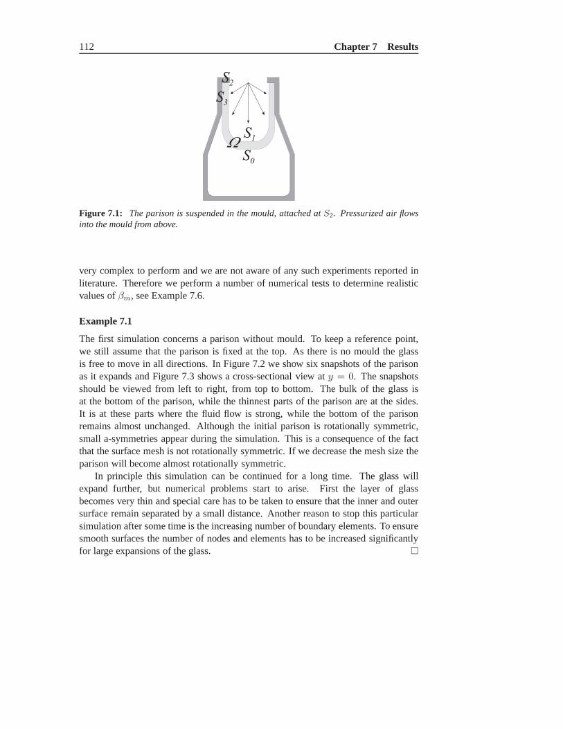
112 Chapter 7 Results
S 0
S 1
S 3
S 2
W
Figure 7.1: The parison is suspended in the mould, attached atS2. Pressurized air flowsinto the mould from above.
very complex to perform and we are not aware of any such experiments reported inliterature. Therefore we perform a number of numerical tests to determine realisticvalues ofβm, see Example 7.6.
Example 7.1
The first simulation concerns a parison without mould. To keep a reference point,we still assume that the parison is fixed at the top. As there isno mould the glassis free to move in all directions. In Figure 7.2 we show six snapshots of the parisonas it expands and Figure 7.3 shows a cross-sectional view aty = 0. The snapshotsshould be viewed from left to right, from top to bottom. The bulk of the glass isat the bottom of the parison, while the thinnest parts of the parison are at the sides.It is at these parts where the fluid flow is strong, while the bottom of the parisonremains almost unchanged. Although the initial parison is rotationally symmetric,small a-symmetries appear during the simulation. This is a consequence of the factthat the surface mesh is not rotationally symmetric. If we decrease the mesh size theparison will become almost rotationally symmetric.
In principle this simulation can be continued for a long time. The glass willexpand further, but numerical problems start to arise. First the layer of glassbecomes very thin and special care has to be taken to ensure that the inner and outersurface remain separated by a small distance. Another reason to stop this particularsimulation after some time is the increasing number of boundary elements. To ensuresmooth surfaces the number of nodes and elements has to be increased significantlyfor large expansions of the glass.

Section 7.1 Glass blowing 113
Example 7.2
The next simulation shown in Figure 7.4 and 7.5 concerns a parison that is suspendedin a mould. The air that flows in in from above causes the glass to take the shape ofthe mould. When the glass touches the wall of the mould, it remains connected to themould, though it is allowed to slip along the mould. In this example we takeβm = 1.The mould has a cylindrical shape with rounded corners. The reason to choose forrounded corners is twofold. First, in practice the corners of a bottle or jar are never90-degree corners. Second, it turns out that it is very hard to make the glass fill thewhole mould if the corners are straight. Even with rounded corners we still need torefine the mesh sufficiently to fill the corners with glass.
The cross-sectional view in Figure 7.5 shows that we get sharp corners at the topof the parison where the surface partsS1 andS2 touch. This is a direct consequenceof the choice to keep the glass fixed atS2, while it is allowed to move atS1. In realitythese sharp corners do not appear.
Example 7.3
Figure 7.6 and 7.7 show a simulation with a slightly more advanced mould. Thelower part of the mould has a smaller width than the upper partof the mould. Againthe corners are rounded and the glass is allowed to slip alongthe wall of the mould.In the previous two simulations the only driving force was the pressure of the air thatis blown into the mould from above. In reality, in first instance the glass is subjectedto gravity only. The glass will sag to the bottom of the mould and when it almosttouches the bottom, air starts to blow into the mould. The simulation in Figure 7.6and 7.7 distinguishes these two stages. The first three snapshots correspond to thesagging stage while the last three snapshots correspond to the blowing stage.
Example 7.4
The simulation that is presented in Figure 7.8 and 7.9 involves a parison and a mouldthat are not rotationally symmetric. We opt for square shapes with rounded corners.Hence the parison and mould are symmetric in the planesx = 0 andy = 0. Howeverthese symmetries are not exploited in the computations. Again we consider the twostages that occur in the production process: sagging and blowing. The first threesnapshots correspond to the sagging stage while the last three snapshots correspondto the blowing phase. In this case it is clearly visible that the glass moves only invertical directionduring the sagging stage. In the blowingstage the glass also movesin radial direction.

114 Chapter 7 Results
Figure 7.2: 3D Snapshots of the glass as it expands due to the air blowing in from above.For this simulation no mould is present, so the glass can expand freely in all directions. Theonly restriction is that the glass is fixed at the top of the parison.

Section 7.1 Glass blowing 115
−1 0 1
−1.5
−1
−0.5
0
−1 0 1
−1.5
−1
−0.5
0
−1 0 1
−1.5
−1
−0.5
0
−1 0 1
−1.5
−1
−0.5
0
−1 0 1
−1.5
−1
−0.5
0
−1 0 1
−1.5
−1
−0.5
0
Figure 7.3: Cross-sectional view of Figure 7.2 aty = 0.

116 Chapter 7 Results
Figure 7.4: 3D Snapshots of the glass as it expands due to the air blowing in from above.The mould has a cylindrical shape with rounded corners. The glass is allowed to slip alongthe wall.

Section 7.1 Glass blowing 117
−0.5 0 0.5
−1
−0.5
0
−0.5 0 0.5
−1
−0.5
0
−0.5 0 0.5
−1
−0.5
0
−0.5 0 0.5
−1
−0.5
0
−0.5 0 0.5
−1
−0.5
0
−0.5 0 0.5
−1
−0.5
0
Figure 7.5: Cross-sectional view of Figure 7.4 aty = 0.
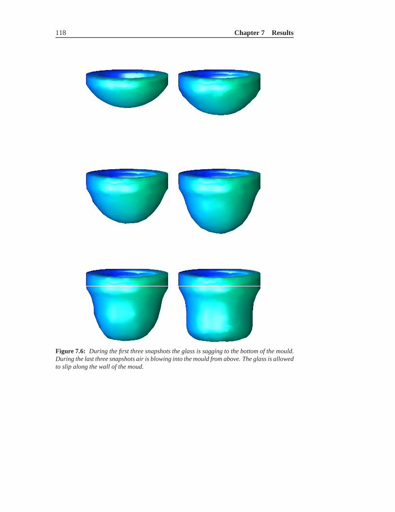
118 Chapter 7 Results
Figure 7.6: During the first three snapshots the glass is sagging to the bottom of the mould.During the last three snapshots air is blowing into the mouldfrom above. The glass is allowedto slip along the wall of the moud.

Section 7.1 Glass blowing 119
−1 0 1
−1.5
−1
−0.5
0
−1 0 1
−1.5
−1
−0.5
0
−1 0 1
−1.5
−1
−0.5
0
−1 0 1
−1.5
−1
−0.5
0
−1 0 1
−1.5
−1
−0.5
0
−1 0 1
−1.5
−1
−0.5
0
Figure 7.7: Cross-sectional view of Figure 7.6 aty = 0.

120 Chapter 7 Results
Figure 7.8: A square parison with rounded corners and a square mould withroundedcorners. During the first three snapshots the glass is sagging to the bottom of the mould.During the last three snapshots air is blowing into the mouldfrom above. The glass is notallowed to slip along the wall.

Section 7.1 Glass blowing 121
−0.5 0 0.5
−1
−0.5
0
−0.5 0 0.5
−1
−0.5
0
−0.5 0 0.5
−1
−0.5
0
−0.5 0 0.5
−1
−0.5
0
−0.5 0 0.5
−1
−0.5
0
−0.5 0 0.5
−1
−0.5
0
Figure 7.9: Cross-sectional view of Figure 7.8 aty = 0.

122 Chapter 7 Results
−1 −0.8 −0.6 −0.4 −0.2 0 0.2 0.4 0.6 0.8 1−1
−0.9
−0.8
−0.7
−0.6
−0.5
−0.4
−0.3
−0.2
−0.1
0
0.1
x
t=0.0
t=1.0
t=3.5
(a) Rotationally symmetric
−1 −0.5 0 0.5 1−1
−0.9
−0.8
−0.7
−0.6
−0.5
−0.4
−0.3
−0.2
−0.1
0
0.1
x
t=1.0
t=4.5
t=0.0
(b) With dent
Figure 7.10: Comparison between a rotationally symmetric parison and a parison with adent. The parisons are shown at three different time levels:t = 0.0, t = 1.0 andt = tend.
Example 7.5
In Figure 7.10 we show the cross-sections of two parisons that are blown into amould. The parison at the left-hand side, which we call parison 1, is perfectlyrotationally symmetric, while the parison at the right-hand side, which we callparison 2, has a dent in the initial shape (at the right-hand side of the parison). Lettend represent the (dimensionless) time level at which the glassproduct is finished,i.e. when the glass more or less covers the wall of the whole mould.
We compare the evolution of the two parisons at three different time levels:t = 0.0, t = 1.0 and t = tend. The value oftend differs for the two simulations.For parison 1 we findtend = 3.5 while parison 2 hastend = 4.5. Parison 2 takesapproximately28.9% longer to finish.
The dent is still present in the final product. The glass layerat the lower rightcorner of parison 2 is thinner than the glass layer at the samelocation of parison 1.Moreover the the glass layer at the lower left corner of parison 2 is thicker than theglass layer at the same location of parison 1. This is caused by the fact that the thinparts of the glass are easier to move than the thick parts. Hence the flow at the dentis relatively large. Since the total amount of glass needs tostay constant, the flow atother parts is relatively small. This is exactly what happens at the lower left cornerof parison 1.

Section 7.2 Curvature driven flow 123
7.2 Curvature driven flow
In the absence of external forces, droplets of viscous fluid tend to evolve to a perfectsphere, regardless of the initial shape of the fluid. This is explained as follows. Amolecule in the interior of the fluid is completely surrounded by other molecules. Itexperiences an attraction from all neighbouring molecules, which sums to zero. Onthe other hand, a molecule that is at the surface of the fluid experiences a net inwardattraction. When the curvature of a convex surface is large,the inward attractionis large and when the curvature is small also the inward attraction is small. Thisintroduces a potential energy of the fluid, which may be transformed to kinetic energy.For a spherically shaped fluid, the curvature is equal at eachpoint of the surface.Hence the inward attraction is the same at each point. The fluid is in an equilibriumstate and the potential energy will not be transformed to kinetic energy. In this sectionwe show that the BEM model developed in Chapter 6 is also applicable for this typeof evolution processes. Related work on two-dimensional fluid domains can be foundin literature [78, 79, 94], in which both the direct and the indirect formulation of theBEM are used.
In this section we illustrate the evolution of viscous dropsby looking at a numberof fluid shapes that evolve to a sphere due to the surface tension. Using the notationfrom Chapter 6, we haveS1 = S2 = S3 = ∅ andS ≡ S0, i.e. the fluid surface is afree surface. The boundary condition for this surface reads
σn = −(αz + βκ)n. (7.2)
Since we do not want to take gravitational effects into account we takeα = 0, and asthe only driving force of the flow is the surface tension, we may setβ = 1.
Note that the choiceS ≡ S0 implies that we have to solve a Neumann problem.Hence we use the deflated form of the boundary integral operator H, as is describedin Section 6.3.
Example 7.6
In Figure 7.11 we see a beam-shaped volume of fluid evolving toa sphere. Figure7.13(a) shows a cross-sectional view aty = 0 of the same fluid. The dimensions ofthe beam are2, 2 and1. The corners of the initial beam are rounded, as a viscous fluidwill never have straight corners. For this particular simulation the initial number ofnodes at the surface isN = 500 and the number of triangular elements isK = 996.The initial volume of the beam is20.6465 and the volume of the final sphere to whichit evolves is20.6355. Hence we have a volume loss of less than0.1%. Since the fluidapproaches a sphere we can compute the radius that such a volume requires to findr = 1.702. The average radius of the nodes at the final surface is1.714 with standard

124 Chapter 7 Results
Figure 7.11: A beam with sizes2, 2 and1 evolves to a sphere.

Section 7.2 Curvature driven flow 125
Figure 7.12: An ellipse with semi-axes of length3, 2 and1 evolves to a sphere.

126 Chapter 7 Results
−2 −1 0 1 2
−1.5
−1
−0.5
0
0.5
1
1.5
x
z
(a) Beam
−3 −2 −1 0 1 2 3
−2
−1.5
−1
−0.5
0
0.5
1
1.5
2
x
z
(b) Ellipse
Figure 7.13: Cross-sectional views of Figure 7.11 and 7.12 aty = 0.
0 5 10 15 20 25 30−0.2
−0.15
−0.1
−0.05
0
0.05
0.1
0.15
0.2
0.25
0.3
time step
mas
s ch
ange
[%]
Figure 7.14: Volume change of the ellipsoid while evolving to a sphere.
deviation0.025, which implies that the final surface is indeed a sphere with almostthe appropriate radius. During the simulation we apply a remeshing technique thatassures that all edges of the boundary elements are smaller than0.39. This leads to afinal discretisation withN = 684 nodes andK = 1364 elements.
Example 7.7
In the next example we watch an ellipsoidal volume of fluid evolve to a sphere(Figures 7.13(b) and 7.12). The initial ellipsoid has semi-axes of length3, 2 and1and hasN = 500 nodes andK = 996 elements at its surface. The volume of the

Section 7.2 Curvature driven flow 127
initial ellipse is equal to24.56 while the volume of the final sphere is equal to24.54.Hence the volume change is0.08%. During the simulation we apply a remeshingtechnique that assures that all edges of the boundary elements are smaller than0.4.This leads to a final discretisation withN = 666 nodes andK = 1328 elements. InFigure 7.14 we show the relative volume change of the ellipsoid during its evolutionto a sphere. We observe that the volume first increases while later on it decreasesagain.
In Section 6.5 we mentioned two types of smoothing techniques to improvethe quality of the BEM solution. We use Example 7.6 to study the effect of thesesmoothing techniques and to determine optimal settings forthe smoothing.
The first technique is Laplacian smoothing, see Appendix C.1. This techniquesmooths the discretised surface and involves two parameters; the number of iterationsN1 and the weightw1. The second technique is the smoothing of a vector field at asurface, see Appendix C.3. This technique smooths the velocity field that is thesolution of the Stokes equations. Involved are also two parameters; the number ofiterationsN2 and the weightw2.
Similar to Example 7.6 we let a beam-shaped volume of fluid evolve to a sphere.We vary the smoothing parameters and determine for which values the final fluidapproximates a sphere optimally.
The initial beam-shaped fluid has a volume of20.6. When the radius of the finalsphere is equal toR := 1.702, the sphere volume is also20.6. This gives us a criterionto determine whether the discretised surface approximatesa sphere accurately. Wecompute the distance of each node at the surface to the geometric center of the fluid.The average of these values should approximate1.702. We also compute the standarddeviation of these values. If the standard deviation is low,the fluid is close to a sphere.In this way we can study the effect of the smoothing techniques on the final geometry.
In the first test we choosew1 = w2 = 0.4 and vary the number of iterations.The results are shown in Table 7.1(a). We see that the averageradius is close to theexact value in each case. The standard deviation is minimal forN1 = N2 = 3. In thesecond test we chooseN1 = N2 = 3, i.e. the optimal choice from the previous test,and vary the weightsw1 andw2. The results are shown in Table 7.1(b). We observethat the best results are obtained whenw1 = w2 = 0.1. In this case the radius isclosest to the exact radius and the standard deviation is minimal.
Until now we chose the same number of iterations and weights for bothsmoothing techniques. In the next test we choosew1 = w2 = 0.1 and we takeseveral combinations of numbers of iterationsN1 andN2. The results are shown inTable 7.2(a). Clearly the effect of the velocity smoothing is smaller than the effect ofLaplacian smoothing.
In the last test we do not perform velocity smoothing (N2 = 0) and we choose

128 Chapter 7 Results
N1 N2 r std(r)
0 0 1.7100 0.05501 1 1.7080 0.01623 3 1.7093 0.01396 6 1.7074 0.0213
w1 w2 r std(r)
0.1 0.1 1.7081 0.01100.4 0.4 1.7093 0.01390.7 0.7 1.7096 0.01541.0 1.0 1.7124 0.0242
Table 7.1: The mean radius and standard deviation of all nodes at the surface of the spherefor (a) w1 = w2 = 0.4 and(b) N1 = N2 = 3.
N1 N2 r std(r)
3 3 1.7090 0.01241 3 1.7131 0.01453 1 1.7081 0.01143 0 1.7081 0.01056 0 1.7085 0.0166
w1 r std(r)
0.1 1.7081 0.01050.2 1.7078 0.01690.3 1.7071 0.00970.4 1.7089 0.01800.6 1.7115 0.0218
Table 7.2: The mean radius and standard deviation of all nodes at the surface of the spherefor (a) w1 = w2 = 0.1 and(b) N1 = 3 andN2 = 0.
N1 = 3. We let the weightw1 vary. The results are shown in Table 7.2(b). We seethat the best results are obtained whenw1 = 0.3. In this case the average radius isvery close to the exact radius and the standard deviation is minimal.
The main conclusions from these tests on smoothing techniques are:
• Velocity smoothing has less effect than Laplacian smoothing;
• The optimal number of iterations for Laplacian smoothing isN1 = 3;
• The optimal weight for Laplacian smoothing isw1 = 0.3.
In all simulations presented in this chapter we perform the smoothing techniques withthe settings equal to or close to the optimal settings listedabove.
7.3 Parameter analysis
In this section we investigate the role of several model parameters for the glassblowing problem. To this end we simulate the flow of a cup-shaped amount of glass.

Section 7.3 Parameter analysis 129
Example 7.8
In the first example we let gravity act on the glass, which willcause the glass to sagdownward. We study the significance of the surface tension during this process. Theeffect of surface tension is represented by the value of the dimensionless numberβ,which involves the surface tension. As gravity is the driving force we setα = 1. Thevalues ofβ that we use in this example lie in the range of0.0 to 0.4. If β = 0.0, thenthe glass does not have surface tension. A large positive value ofβ implies a highsurface tension.
We let the glass sag downwards for a fixed amount of time and plot the resultingshape in Figure 7.15. We do this for several values ofβ. The left pane of the figuregives a cross-section of the glass, while the right pane zooms in on the lowest part ofthis cross-section. Several lines are plotted, each representing a specific value ofβ.In the left pane, the various shapes, corresponding to the various values ofβ, moreor less coincide. In the right pane we are able to distinguishthe various shapes. Weobserve that the glass flow has moved downward the furthest for β = 0.0, while forlarge values ofβ the glass has not moved very far. Hence the surface tension slowsdown the flow of the glass.
Table 7.3 gives the height of the lowest point of the glass surface for severalvalues ofβ. We compare these heights with the height forβ = 0.0. We observe that,for β = 1.0, the glass surface is more than2% higher than forβ = 0.0. Hence thesurface tension plays a small role in the case of gravity driven flow. Therefore weinclude surface tension in all numerical simulations that cover the sagging stage.
β zmin difference (%)0.0 −0.8970 –0.1 −0.8908 +0.690.2 −0.8858 +1.250.3 −0.8813 +1.750.4 −0.8765 +2.29
Table 7.3: Thez-coordinate of the lowest node after sagging for several values of the surfacetensionβ.
Example 7.9
In the next example we investigate the significance of the surface tension during theblowing stage. Hence the glass does not sag due to gravity in this case, but it flowsdue to a pressure difference between upper and lower layer ofthe glass. In this case
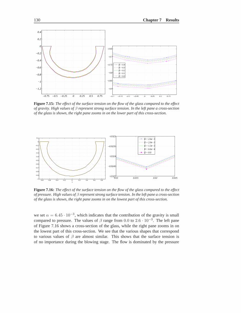
130 Chapter 7 Results
−0.75 −0.5 −0.25 0 0.25 0.5 0.75
−1.2
−1
−0.8
−0.6
−0.4
−0.2
0
0.2
0.4
−0.2 −0.15 −0.1 −0.05 0 0.05 0.1 0.15
−0.9
−0.85
−0.8
−0.75
−0.7
−0.65
β = 0.4β = 0.3β = 0.2β = 0.1β = 0.0
Figure 7.15: The effect of the surface tension on the flow of the glass compared to the effectof gravity. High values ofβ represent strong surface tension. In the left pane a cross-sectionof the glass is shown, the right pane zooms in on the lower partof this cross-section.
−0.8 −0.6 −0.4 −0.2 0 0.2 0.4 0.6 0.8−1
−0.9
−0.8
−0.7
−0.6
−0.5
−0.4
−0.3
−0.2
−0.1
0
0.1
x
0.01 0.015 0.02 0.025−0.925
−0.9245
−0.924
−0.9235
−0.923
β = 2.6e−3
β = 2.0e−3
β = 1.3e−3
β = 6.6e−4
β = 0.0
Figure 7.16: The effect of the surface tension on the flow of the glass compared to the effectof pressure. High values ofβ represent strong surface tension. In the left pane a cross-sectionof the glass is shown, the right pane zooms in on the lowest part of this cross-section.
we setα = 6.45 · 10−3, which indicates that the contribution of the gravity is smallcompared to pressure. The values ofβ range from0.0 to 2.6 · 10−3. The left paneof Figure 7.16 shows a cross-section of the glass, while the right pane zooms in onthe lowest part of this cross-section. We see that the various shapes that correspondto various values ofβ are almost similar. This shows that the surface tension isof no importance during the blowing stage. The flow is dominated by the pressure
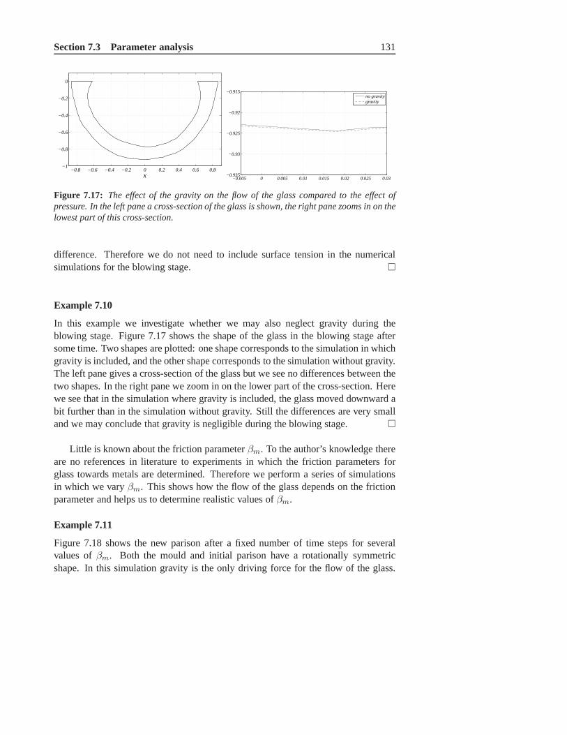
Section 7.3 Parameter analysis 131
−0.8 −0.6 −0.4 −0.2 0 0.2 0.4 0.6 0.8−1
−0.8
−0.6
−0.4
−0.2
0
x
−0.005 0 0.005 0.01 0.015 0.02 0.025 0.03−0.935
−0.93
−0.925
−0.92
−0.915
no gravitygravity
Figure 7.17: The effect of the gravity on the flow of the glass compared to the effect ofpressure. In the left pane a cross-section of the glass is shown, the right pane zooms in on thelowest part of this cross-section.
difference. Therefore we do not need to include surface tension in the numericalsimulations for the blowing stage.
Example 7.10
In this example we investigate whether we may also neglect gravity during theblowing stage. Figure 7.17 shows the shape of the glass in theblowing stage aftersome time. Two shapes are plotted: one shape corresponds to the simulation in whichgravity is included, and the other shape corresponds to the simulation without gravity.The left pane gives a cross-section of the glass but we see no differences between thetwo shapes. In the right pane we zoom in on the lower part of thecross-section. Herewe see that in the simulation where gravity is included, the glass moved downward abit further than in the simulation without gravity. Still the differences are very smalland we may conclude that gravity is negligible during the blowing stage.
Little is known about the friction parameterβm. To the author’s knowledge thereare no references in literature to experiments in which the friction parameters forglass towards metals are determined. Therefore we perform aseries of simulationsin which we varyβm. This shows how the flow of the glass depends on the frictionparameter and helps us to determine realistic values ofβm.
Example 7.11
Figure 7.18 shows the new parison after a fixed number of time steps for severalvalues ofβm. Both the mould and initial parison have a rotationally symmetricshape. In this simulation gravity is the only driving force for the flow of the glass.

132 Chapter 7 Results
−0.8 −0.6 −0.4 −0.2 0−1
−0.9
−0.8
−0.7
−0.6
−0.5
−0.4
−0.3
−0.2
−0.1
0
x0.5 0.6 0.7 0.8 0.9
−0.65
−0.6
−0.55
−0.5
−0.45
−0.4
−0.35
−0.3
−0.25
−0.2
−0.15
x
βm
= 5.0
βm
= 3.0
βm
= 2.0
βm
= 1.5
Figure 7.18: Deformation of the glass after a fixed number of time steps fordifferent valuesof βm.
Theoretically, forβm = ∞ the friction between glass and mould is infinitely largeand the glass does not slip at all along the wall of the mould; for βm = 0 there is nofriction, and the glass can flow freely along the wall of the mould. We observe that forβm = 5 the glass has slipped a little along the wall of the mould. This slip becomeslarger if the friction parameter is lowered further. Forβm = 2 andβm = 1.5 we seethat the glass that is in contact with the wall moves faster downward than the glassthat does not touch the wall. Hence these values ofβm are not realistic. Appropriatechoices forβm lie in the range of3 to∞. Note that we use the dimensionless frictionparameter here, which depends on the length scale and the viscosity. Hence forexamples that have other characteristic lengths and viscosities, suitable values forβm may be slightly different than the values that we find for thisexample.
Example 7.12
Example 7.11 shows that a minimal value for the friction parameter isβm = 3, basedon observations of intermediate shapes during sagging. In the current example weelaborate a bit more on values ofβm that are in the interval[5,∞). For severalvalues ofβm we simulate the blowing stage and plot the final shapes in Figure 7.19.We observe that the shapes vary significantly.
In Table 7.4 we give the height of the lowest point of the glasssurface for several

Section 7.3 Parameter analysis 133
−0.8 −0.6 −0.4 −0.2 0 0.2 0.4 0.6 0.8
−1
−0.8
−0.6
−0.4
−0.2
0
x
βm = ∞
βm = 30
βm = 15
βm = 10
βm = 5
Figure 7.19: The effect of friction on the flow of the glass compared to the effect of pressure.High values ofβm represent much friction.
βm zmin difference (%)∞ −0.90 –30 −1.05 −615 −1.09 −910 −1.12 −125 −1.17 −18
Table 7.4: Thez-coordinate of the lowest node after the blowing stage for several values ofthe friction parameterβm.
values ofβm. We compare these heights with the height forβm = 0. We see thatβm = 5 gives a glass surface that is18% lower than the surface forβm = ∞. Hencethe friction between glass and mould is very important and cannot be neglected.

Appendix A
Curvature approximation
This appendix describes the approximation of curvature parameters of a discretisedsurface. When a surface is given by a parametric representation these curvatureparameters can be calculated analytically. However in manynumerical applicationsthe surface is a discretised surface, consisting of a large number of triangular elementsand nodes. For such discretised surfaces it is not so straightforward to computecurvature parameters. However, there exists a number of strategies to approximatecurvature parameters, of which theparaboloid fit methodappears to be the mostaccurate one [89]. We use a similar method in which abicubic polynomial is fittedthrough data points.
Assume that a surfaceS is uniquely described byz = f(x, y), where(x, y) is ina closed and bounded setD ⊂ R
2. TheGaussian curvatureof the surface at a point(x, y) ∈ D is defined as
K :=fxxfyy − f2
xy
(1 + f2x + f2
y )2
∣∣∣(x,y)
, (A.1)
and themean curvatureas
H :=(1 + f2
x)fxx − 2fxfyfxy + (1 + f2y )fyy
2(1 + f2x + f2
y )3/2
∣∣∣(x,y)
. (A.2)
Related to these two curvature parameters are theprincipal curvaturesκ1 andκ2.They satisfy the relations
K = κ1κ2, H =1
2(κ1 + κ2). (A.3)
The principal curvatures can also be found as follows. Letx be a point at thesurfaceS and let a vertical plane intersect the surface in the pointx. The intersectionof the surface and the plane yields a curveC. By rotating the planes around the
134

135
Figure A.1: The nodesv0 andv1, . . . ,vm are translated and rotated in such a way thatv isin the origin and its normal vector points in the vertical direction.
vertical axis we get a set of curvesC. For each curve we calculate its the secondderivative at the pointx. The largest second derivative is the largest principalcurvatureκ1 and the smallest second derivative is the smallest principal curvatureκ2.
The triangulated surfaceT is described by a set of nodesxp at the surfaceS,p = 1, . . . , N and a set of trianglesTk, k = 1, . . . ,K, each triangle defined bythree nodes. We want to approximate the curvature in each node xp using only theinformation of the locations of neighbouring nodes. A node is a neighbour ofxp
if they share a triangleTk. The procedure to approximate the curvature goes asfollows. Let v0 be the node at which we want to approximate the curvature. Letv1, . . . ,vm be them neighbouring nodes ofv0. First we translate and rotate thenodesv0,v1, . . . ,vm in such a way thatv0 is translated to the origin and the normalvector inv0 at the surface points in vertical direction, see Figure A.1.Note that atranslation and rotation of the surface does not affect the curvature parameters.We fit a bicubic polynomialp(x, y) through the nodesv0,v1, . . . ,vm using a leastsquares technique. The translation and rotation of the nodes guarantees that such apolynomial exists. The polynomial provides a local parameterisation of the surfaceof the formz = p(x, y). Hence we can use (A.1) and (A.2) to calculate the curvatureparameters in(x, y) = (0, 0) at the parametric surfac.
We describe the procedure above in more detail. Define the edge betweenv0 andvi by ei := v0 − vi, i = 1, . . . ,m. Let thek-th triangle be given by the nodesv0, vk1 andvk2. For the outward normal at this triangle we use the straightforwarddefinition,
nk :=ek1 × ek2
‖ek1 × ek2‖ . (A.4)
The normal vector at the pointv0 can be defined in several ways. In each case thenormal vector atv0 is a weighted sum of the normals at the surrounding triangles.For the weights several options are available.

136 Appendix A Curvature approximation
1. Average of normals at surrounding triangles,
n :=1
m
m∑
k=1
nk. (A.5)
2. If Ak is the area of thek-th triangle,
n :=m∑
k=1
1
Aknk. (A.6)
3. Define the weightθk by
cos θk :=〈ek1 ,ek2〉‖ek1‖‖ek2‖ , (A.7)
i.e. the angle between the two edges of a triangle that meet inv0, and
n :=
m∑
k=1
θknk. (A.8)
Later on we will demonstrate the effect of the different definitions of n on thecurvature approximation. It turns out that the last definition gives the most accurateapproximation.
We want to rotate the nodesv0,v1, . . . ,vm such that the normal inv0 pointsin either positive or negative vertical direction. For thisgoal we define two rotationmatrices
R0 :=
cosα1 0 − sinα1
0 1 0sinα1 0 cosα1
, R1 :=
1 0 00 cosα2 − sinα2
0 sinα2 cosα2
, (A.9)
which rotate the nodes over an angleα1 with respect to they-axis and over an angleα2 with respect to thex-axis respectively. Writen = [n1, n2, n3]
T and denote therotation ofn overα1 by n1 := R0n. We writen1 = [n1
1, n12, n
13]
T and denote therotation ofn1 overα2 byn2 := R1n
1. It can be shown thatn2 points in positive ornegativez-direction ifα1 andα2 are chosen as follows,
α1 =
arctan(n1
n3) if n3 6= 0,
π2 if n3 = 0,
α2 =
− arctan(n1
2
n13
) if n13 6= 0,
π2 if n1
3 = 0.(A.10)

137
Having determined the appropriate rotation anglesα1 andα2, we can rotate all nodesv0,v1, . . . ,vm, using the rotation matrixP := R1R0. This yields a set of newnodes,
w0 := Pv0,
wi := Pvi, i = 1, . . . ,m. (A.11)
It may occur that at this stage the normal vector atw0 is pointing in the positivez-direction. In that case we simply mirror all nodes with respect to the(x, y)-plane.Thus the normal atw0 always point in the negativez-direction. Finally we translateall nodes over the same distance such thatw0 is located in the origin. This yields thefollowing set of nodes,
w0 := w0 − w0 = 0,
wi := wi − w0, i = 1, . . . ,m. (A.12)
Let p(x, y) := a1x2 + a2xy + a3y
2 + a4x3 + a5y
3 be a bicubic polynomial. Theequationz = p(x, y) describes a 2D surface. We use a linear least squares techniqueto find the polynomialp that gives the best fit of the nodesw0,w1, . . . ,wm. Inthis way we create a parametric representation of a surface that locally approximatesthe discretised surfaceS. The Gaussian and mean curvature at the nodev0 of thediscretised surface are obtained by evaluating (A.1) and (A.2) with f ≡ p at thepoint (x, y) = (0, 0). They can be expressed in terms of the coefficients of thepolynomialp,
K = 4a1a3 − a22,
H = a1 + a3. (A.13)
We illustrate the procedure to approximate the curvature ofa discretised surface fora sphere and an ellipsoid.
Example A.1
In Figure A.2(a) we show a unit sphere discretised withN = 704 nodes. It can beshown that the unit sphere has a Gaussian curvature equal to1 in each point at thesurface. The color at the surface represents the value of theGaussian curvature asapproximated by the polynomial fit method. We observe that the approximation isnot equal to1 everywhere.
We repeat the curvature approximation for the unit sphere with other numbers ofnodesN . In Figure A.2(b) we show the maximum and mean error of the curvatureapproximation as a function of number of nodesN . To our surprise the mean errordoes not decrease if the number of nodes increases, i.e. the discretisation refines.Moreover the maximal error is even increasing with the number of nodes.

138 Appendix A Curvature approximation
0.75
0.8
0.85
0.9
0.95
1
1.05
1.1
(a) A discretised sphere withN = 704 nodes.Color represents the Gaussian curvature.
300 400 500 600 700 8000
5
10
15
20
25
30
N
err
or
(%)
max errormean error
(b) The maximal and mean error in the curvatureapproximation of a sphere as a function of numberof nodesN .
Figure A.2: Gaussian curvature approximation for a sphere. All neighbouring nodes areused in the approximation.
1.005
1.01
1.015
1.02
1.025
1.03
1.035
1.04
(a) A discretised sphere withN = 704 nodes.Color represents the Gaussian curvature.
300 400 500 600 700 8000
1
2
3
4
5
6
N
err
or
(%)
max errormean error
(b) The maximal and mean error in the curvatureapproximation of a sphere as a function of numberof nodesN .
Figure A.3: Gaussian curvature approximation for a sphere. Only the fivenearestneighbouring nodes are used in the approximation.

139
1.015
1.02
1.025
1.03
Figure A.4: A sphere with a more regular discretisation. Color represents the Gaussiancurvature.
max nr. of neighbours max. error(%) mean error(%)
4 4.08 1.88
5 4.08 1.70
6 29.18 5.86
7 29.18 5.54
8 29.18 5.62
all 29.18 5.62
Table A.1: The maximal and mean error in the curvature approximation when a certainnumber of neighbours is used for creating a polynomial fit.
Example A.2
The way to improve the curvature approximation is by using only the nearestneighbours of a node when constructing the bicubic polynomial. In Figure A.3we show the curvature approximation when at most five neighbours are used. Wesee that the errors are much smaller and that the accuracy increases when we takemore nodes. We also investigate what number of neighbours gives the best curvatureapproximation. In Table A.1 we give the maximal and mean error when a certainnumber of neighbours is used. We see that for five neighbours the approximation isthe most accurate.

140 Appendix A Curvature approximation
weight max. error(%) mean error(%)1m 57.08 7.351
Ak36.27 5.94
θk 4.08 1.70
Table A.2: The maximal and mean error in the curvature approximation for a sphere foreach of the three definitions of the normal at a node. Number ofnodes isN = 704.
Example A.3
The accuracy of the curvature approximation also depends onthe discretisation of thesurface. In Figure A.3 we see that the largest errors are at the top of the sphere, wherewe have a number of narrow triangular elements. In Figure A.4we show a spherewith a more regular discretisation, i.e. all elements have approximately the sameshape and size. Although the accuracy is more or less the sameas for the sphere inFigure A.3, the largest errors are not concentrated at one area.
Example A.4
We mentioned that there are several possibilities to define the normal vector at a node.In Table A.2 we show the maximal and mean error in the curvature approximationfor each of the three definitions. It is clear that the definition in which we use theweightsθk results in a higher accuracy.
Also for an ellipsoid the Gaussian curvature can be calculated explicitly. For apoint (x, y, z) at the surface of the ellipsoid the Gaussian curvature is given by
K =1
a2b2c2
(x2
a4+y2
b4+z2
c4
)−2
, (A.14)
wherea, b andc are the lengths of the semi-axes.
Example A.5
In Figure A.5(a) we show an ellipsoid where the semi-axes have length3, 2 and1, discretised withN = 932 nodes. The color at the surface represents theGaussian curvature of the surface. We see that at the tipsx ± 3 the curvature ismaximal, which agrees with the maximal value of the analyticexpression forK. Werepeat the curvature approximation for the ellipsoid with other numbers of nodesN .In Figure A.5(b) we give the maximal error and the mean error of the curvature

141
0.2
0.4
0.6
0.8
1.0
1.2
1.4
1.6
1.8
2.0
(a) A discretised ellipsoid withN = 932 nodes.Color represents the Gaussian curvature.
400 500 600 700 800 9003
4
5
6
7
8
9
N
err
or
(%)
max errormean error
(b) The maximal and mean error in the curvatureapproximation of the ellipsoid as a function ofnumber of nodesN .
Figure A.5: Gaussian curvature approximation for an ellipsoid. Only the five nearestneighbouring nodes are used in the approximation.
approximation as a function ofN . We see that for a fine discretisation of the surface(N > 550) the mean error is lower than5%.
Appendix B
Contact problem
In this appendix we address the contact problem of a fluid witha wall. In manymathematical models for fluid flow it is assumed that the fluid is already in contactwith a wall. At the contact area a slip or no-slip boundary condition is prescribedthat ensures that the fluid remains in contact with the wall. For the blowing problemcovered in this thesis the fluid may, in first instance, not yetbe in contact with thewall. However as the fluid expands into the direction of the wall, at a certain momentit will touch the wall. From that moment on, the fluid will stayconnected to thewall at that specific point. Thus a fluid particle may at first instance be part of a freeboundary, while some time later it is fixed at a wall (althoughit may slide along thewall in the case of a slip boundary condition).
For a flow that is computed numerically the touching of the wall is difficult toimplement. In boundary element methods, the fluid domain is described by a set ofnodes and elements at the surface of the domain. Moreover thetrajectory of a nodeor fluid particle is only known at a discrete set of time points. Thus it may occurthat at timet = tn a fluid particle is not yet at the wall, while at timet = tn+1 theparticle has moved to the other side of the wall, see Figure B.1. Physically this is notpossible, but it is very difficult to “tell” the fluid particlethat it cannot move throughthe wall.
When an explicit time integration method is used to track theflow of the fluid,e.g. Euler forward, there is a simple way to avoid nodes moving through the wall.One can find an intermediate timetn < t∗ < tn+1 such that the node that crossedthe wall lies exactly at the wall att = t∗. In this way we effectively decrease thetime step of the time integration method to a suitable size. In practice one shouldthus verify all nodes att = tn+1 whether they moved through the wall. The nodethat has moved through the wall the furthest determines the new time step size. Thedrawback of the procedure is that the time steps can become very small, especiallywhen the number of nodes is large.
142
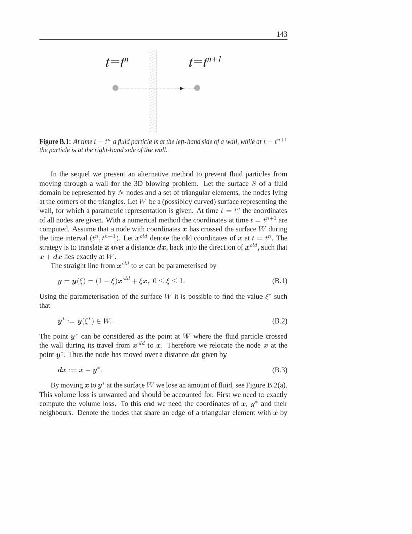
143
t = t n t = t n + 1
Figure B.1: At timet = tn a fluid particle is at the left-hand side of a wall, while att = tn+1
the particle is at the right-hand side of the wall.
In the sequel we present an alternative method to prevent fluid particles frommoving through a wall for the 3D blowing problem. Let the surfaceS of a fluiddomain be represented byN nodes and a set of triangular elements, the nodes lyingat the corners of the triangles. LetW be a (possibley curved) surface representing thewall, for which a parametric representation is given. At time t = tn the coordinatesof all nodes are given. With a numerical method the coordinates at timet = tn+1 arecomputed. Assume that a node with coordinatesx has crossed the surfaceW duringthe time interval(tn, tn+1). Letxold denote the old coordinates ofx at t = tn. Thestrategy is to translatex over a distancedx, back into the direction ofxold, such thatx+ dx lies exactly atW .
The straight line fromxold to x can be parameterised by
y = y(ξ) = (1 − ξ)xold + ξx, 0 ≤ ξ ≤ 1. (B.1)
Using the parameterisation of the surfaceW it is possible to find the valueξ∗ suchthat
y∗ := y(ξ∗) ∈W. (B.2)
The pointy∗ can be considered as the point atW where the fluid particle crossedthe wall during its travel fromxold to x. Therefore we relocate the nodex at thepointy∗. Thus the node has moved over a distancedx given by
dx := x− y∗. (B.3)
By movingx toy∗ at the surfaceW we lose an amount of fluid, see Figure B.2(a).This volume loss is unwanted and should be accounted for. First we need to exactlycompute the volume loss. To this end we need the coordinates of x, y∗ and theirneighbours. Denote the nodes that share an edge of a triangular element withx by

144 Appendix B Contact problem
x
x 1 x 2
d V
y *W
f l u i d
(a) By movingx back to the surfaceW a certainamount of fluid is lost (cross-sectional view).
x
x 1
x 2
x 3
x 4 x 5
e 1e 2
e 3
e 4 e 5
(b) The nodex is surrounded bymtriangular elements andm neighbouringnodes.
Figure B.2: Procedure to relocatex at the wall.
x1, . . . ,xm, see Figure B.2(b). The volume lossdV due to the displacementdx isgiven by [64]
dV =1
6〈dx,
m∑
j=1
ej × ej+1〉. (B.4)
Hereej is the edge connectingx andxj, whereem+1 ≡ e1.For the blowing problem covered in this thesis the fluid domain is in fact a layer
of fluid. For this particular shape we develop a strategy to compensate the volumeloss. In Figure B.3(a) we give a schematic overview of the situation. The nodex islocated at the lower boundary of the fluid and is moved back to the pointy∗ atW .Letw be the node at the upper boundary that is closest toy∗. We replacew over adistancedw such that the volume loss is compensated. It is easy to see that dw hasto satisfy
−dV =1
6〈dw,
m∑
j=1
f j × f j+1〉, (B.5)
wheref j is the edge betweenw and itsj-th neighbour. Note that the vector quantitydw has to satisfy a scalar equation. This means that we have the freedom to choosethe direction ofdw. We choosedw = w0n
w, wherenw is the outward normal atw.If we substitute this into the condition fordw we find
w0 = − 6dV
〈nw,∑m
j=1 fj × f j+1〉 . (B.6)

145
x
y *Ww
n w
f l u i d
(a)
x
y *W
w 4f l u i dw 1 w 2
w 5w 3
(b)
Figure B.3: One or multiple nodes are moved to compensate the volume loss.
In the procedure described above only one nodew is relocated to compensate thevolume loss caused by relocatingx to the wall. The procedure can be improved byrelocating several nodesw1, . . . ,wm, each node compensating a part of the volumeloss. Figure B.3(b) illustrates this idea for a 2D setting. The nodex has movedthrough a wall, which is a curved line at a certain height. We distinguish5 nodeswi
in the neighbourhood ofx that are candidates to be relocated. Letαi be5 weightsthat sum to1. Each of the nodeswi is relocated over a distancedwi following theprocedure described above, with the difference that the volume loss thatwi has tocompensate is multiplied by the weightαi. In this way the amount of fluiddV isdistributed over a larger part of the total fluid, which is physically more correct.
Example B.1
We demonstrate the procedure described in this appendix fora thin layer of fluidthat is slightly curved, see Figure B.4. In this example we only use a single nodeto compensate the volume loss. Located at the right is a straight wall, representedgraphically by the light-gray surface. At timet = tn all nodes at the fluid surfaceare at the left side of the wall (Figure B.4(a)). A numerical method provides thecoordinates of the nodes at the new time levelt = tn+1, see Figure B.4(b). Weobserve that a number of nodes has moved through the wall. We correct this byrelocating these nodes at appropriate points at the wall. Toaccount for the volumeloss, we also relocate a number of nodes that are at the opposite side of the fluid layer.The new situation is shown in Figure B.4(c). We observe that the fluid perfectlytouches the wall.
Figure B.5 shows a cross-section of the situation. The solidline represents thefluid layer, for which some nodes move to the right-hand side of the wall. The wall isrepesented by the vertical dashed line. In the third figure the fluid perfectly touches

146 Appendix B Contact problem
(a) t = tn (b) t = t
n+1 (c) t = tn+1
Figure B.4: A fluid layer near a wall (a). At timet = tn+1 some nodes of the discretisedfluid surface have moved through the wall (b). These nodes arerelocated at the wall.Simultaneously some other nodes at the opposite side of the fluid layer are also relocatedto compensate the volume loss (c).
(a) t = tn (b) t = t
n+1 (c) t = tn+1
Figure B.5: Cross-sectional view of Figure B.4
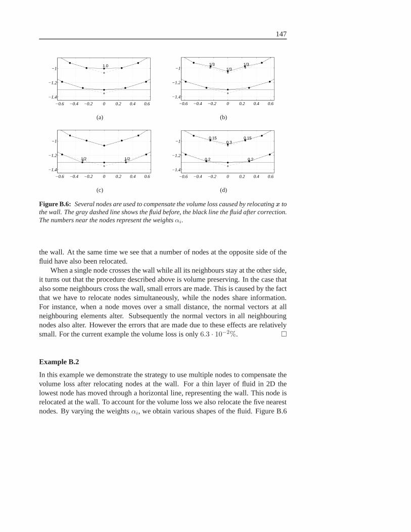
147
−0.6 −0.4 −0.2 0 0.2 0.4 0.6
−1.4
−1.2
−11.0
(a)
−0.6 −0.4 −0.2 0 0.2 0.4 0.6
−1.4
−1.2
−1 1/31/3 1/3
(b)
−0.6 −0.4 −0.2 0 0.2 0.4 0.6
−1.4
−1.2
−1
1/2 1/2
(c)
−0.6 −0.4 −0.2 0 0.2 0.4 0.6
−1.4
−1.2
−1
0.2 0.2
0.30.15 0.15
(d)
Figure B.6: Several nodes are used to compensate the volume loss caused by relocatingx tothe wall. The gray dashed line shows the fluid before, the black line the fluid after correction.The numbers near the nodes represent the weightsαi.
the wall. At the same time we see that a number of nodes at the opposite side of thefluid have also been relocated.
When a single node crosses the wall while all its neighbours stay at the other side,it turns out that the procedure described above is volume preserving. In the case thatalso some neighbours cross the wall, small errors are made. This is caused by the factthat we have to relocate nodes simultaneously, while the nodes share information.For instance, when a node moves over a small distance, the normal vectors at allneighbouring elements alter. Subsequently the normal vectors in all neighbouringnodes also alter. However the errors that are made due to these effects are relativelysmall. For the current example the volume loss is only6.3 · 10−2%.
Example B.2
In this example we demonstrate the strategy to use multiple nodes to compensate thevolume loss after relocating nodes at the wall. For a thin layer of fluid in 2D thelowest node has moved through a horizontal line, representing the wall. This node isrelocated at the wall. To account for the volume loss we also relocate the five nearestnodes. By varying the weightsαi, we obtain various shapes of the fluid. Figure B.6

148 Appendix B Contact problem
present several shapes, each one corresponding to a particular set of weights. Thefirst shape is the result when only the node oppositex is relocated, as we did in theprevious example. Apart for this particular choice, the other shapes only have smalldifferences. It is a matter of taste to determine which shape, i.e. which set of weights,is preferrable.

Appendix C
Smoothing techniques
In this appendix we present a number of smoothing techniques. The smoothing isapplied to a triangulated surface directly, or to a scalar function or vector field at thisdiscretised surface.
C.1 Laplacian smoothing
A well-known technique to smooth a triangulated surface is the technique calledLaplacian smoothing[42, 64, 96]. LetS be a triangulated surface withN nodesandK triangular elements. The idea is that the coordinates of thenodes containnoise due to inaccuracies in the numerical method that determines these coordinates.The noise causes the surface to look unsmooth and irregular.Laplacian smoothingattempts to remove the noise, thus obtaining a smoother surface.
Let x1, . . . ,xm be them neighbours of a nodex, i.e. the nodes that share atriangular element withx. For each nodex we compute the geometric averagexav
of the neighbouring nodes,
xav :=1
m
m∑
i=1
xi. (C.1)
If the nodex is too far away fromxav , it is relocated to a weighted average ofxandxav,
x→ (1 − w)x+ wxav, (C.2)
wherew is a suitably chosen weight,0 ≤ w ≤ 1. In this way x is movednearer toxav. If w = 1, x is placed atxav, if w = 0, x stays at its own place.We can relocate every node at the surface, in which case we apply global smoothing.
149

150 Appendix C Smoothing techniques
Figure C.1: A triangulated sphere whose coordinates contains noise is smoothed to analmost perfect sphere.
We may also replacex only if the distance toxav exceeds a certain tolerance value.In that case we applylocal smoothing. In other words, we smooth the surface only atnodes where it is most needed. For both global and local smoothing, the process canbe repeated several times. In each iteration the surface gets smoother.
A side-effect of the smoothing is that the volume that the surface enclosesdecreases. This is a typical disadvantage of standard Laplacian smoothing. There areseveral modifications to the standard technique to avoid volume loss. The simplestmodification is to restrict the movement of the nodex to a direction perpendicularto the normal at the surface atx. Unfortunately this reduces the performance of thesmoothing. Another possibility is to consider pairs of nodes that are connected by anedge [64]. The two nodes are relocated to new positions simultaneously. In this waywe have more freedom to move the nodes to the desired locations, while conservingthe volume. In the examples of this section we use the latter modification to Laplaciansmoothing.
Example C.1
As an example we consider a triangulated unit sphere, as is shown in Figure C.1.Normally distributed noise is added to the coordinates of the nodes. By applyingseveral iterations of Laplacian smoothing the noise is removed and a smooth surfaceappears.
Example C.2
For the Laplacian smoothing technique three parameters areneeded. The weightw,the number of iterationsn and the type of smoothing, which can be global or local. InFigure C.2 we let these parameters vary and study the performance of the smoothing.Again we consider the example of the noisy unit sphere. Ideally all nodes are at a
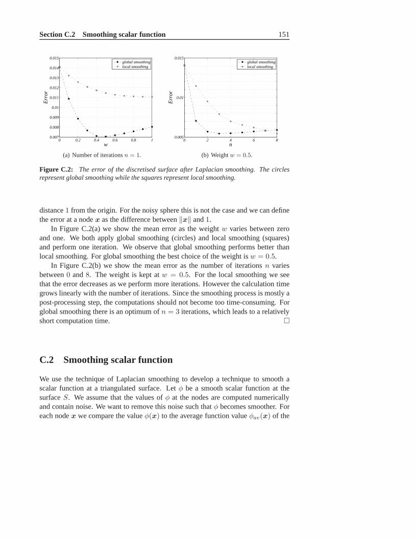
Section C.2 Smoothing scalar function 151
0 0.2 0.4 0.6 0.8 10.007
0.008
0.009
0.01
0.011
0.012
0.013
0.014
0.015
w
Err
or
global smoothinglocal smoothing
(a) Number of iterationsn = 1.
0 2 4 6 80.005
0.01
0.015
n
Err
or
global smoothinglocal smoothing
(b) Weightw = 0.5.
Figure C.2: The error of the discretised surface after Laplacian smoothing. The circlesrepresent global smoothing while the squares represent local smoothing.
distance1 from the origin. For the noisy sphere this is not the case and we can definethe error at a nodex as the difference between‖x‖ and1.
In Figure C.2(a) we show the mean error as the weightw varies between zeroand one. We both apply global smoothing (circles) and local smoothing (squares)and perform one iteration. We observe that global smoothingperforms better thanlocal smoothing. For global smoothing the best choice of theweight isw = 0.5.
In Figure C.2(b) we show the mean error as the number of iterations n variesbetween0 and8. The weight is kept atw = 0.5. For the local smoothing we seethat the error decreases as we perform more iterations. However the calculation timegrows linearly with the number of iterations. Since the smoothing process is mostly apost-processing step, the computations should not become too time-consuming. Forglobal smoothing there is an optimum ofn = 3 iterations, which leads to a relativelyshort computation time.
C.2 Smoothing scalar function
We use the technique of Laplacian smoothing to develop a technique to smooth ascalar function at a triangulated surface. Letφ be a smooth scalar function at thesurfaceS. We assume that the values ofφ at the nodes are computed numericallyand contain noise. We want to remove this noise such thatφ becomes smoother. Foreach nodex we compare the valueφ(x) to the average function valueφav(x) of the

152 Appendix C Smoothing techniques
function at the neighbours ofx,
φav(x) :=1
m
m∑
i=1
φ(xi). (C.3)
The value ofφ atx is replaced by a weighted average ofφ(x) andφav(x),
φ(x) → (1 − w)φ(x) + wφav(x). (C.4)
If we do this for every node we apply global smoothing. We may also decide tochangeφ(x) only if the difference betweenφ(x) andφav(x) is larger than a certaintolerance value. In that case we apply local smoothing. The whole process canbe repeated several times, in each iteration improving the smoothness of the scalarfunctionφ.
Example C.3
To demonstrate the smoothing of a scalar function we consider the unit sphere. Thistime we do not add noise to the coordinates of the nodes of the triangulated sphere,so the sphere is a perfect sphere. As a test function we chooseφ(x) = x + y + zand add normally distributed noise to the function values atthe nodes. In analogy toLaplacian smoothing three parameters exist: the weightw, the number of iterationsn and the type of smoothing, which can be global or local. In Figure C.3 we let theseparameters vary and study the performance of the smoothing.For this goal we definethe following error measure. We consider the vector with exact function values ofφ and the vector with smoothed function values ofφ. Then we determine the meandifference between these two vectors.
In Figure C.3(a) we let the weightw vary between zero and one. We apply globalsmoothing (circles) and local smoothing (squares). As was the case for Laplaciansmoothing, global smoothing gives better results than local smoothing. The optimalchoice forw in the case of global smoothing isw = 0.6. In Figure C.3(b) we letthe number of iterationsn vary between0 and6. We observe thatn = 2 or n = 3iterations of smoothing yield the smallest error.
C.3 Smoothing vector field
In the same way as we smoothed a scalar function at a triangulated surface wemay also smooth a vector field at a surface. Letv be a smooth vector field at thesurfaceS. We assume that for each nodex the vectorv(x) is computed numerically
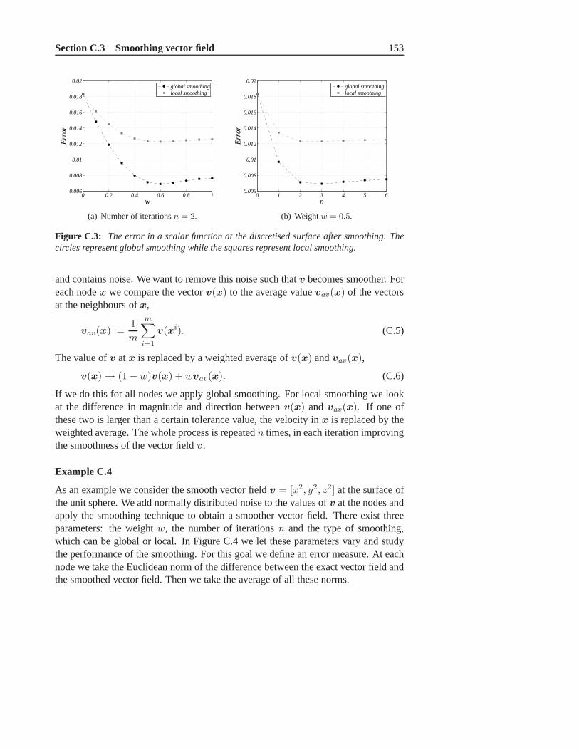
Section C.3 Smoothing vector field 153
0 0.2 0.4 0.6 0.8 10.006
0.008
0.01
0.012
0.014
0.016
0.018
0.02
w
Err
or
global smoothinglocal smoothing
(a) Number of iterationsn = 2.
0 1 2 3 4 5 60.006
0.008
0.01
0.012
0.014
0.016
0.018
0.02
n
Err
or
global smoothinglocal smoothing
(b) Weightw = 0.5.
Figure C.3: The error in a scalar function at the discretised surface after smoothing. Thecircles represent global smoothing while the squares represent local smoothing.
and contains noise. We want to remove this noise such thatv becomes smoother. Foreach nodex we compare the vectorv(x) to the average valuevav(x) of the vectorsat the neighbours ofx,
vav(x) :=1
m
m∑
i=1
v(xi). (C.5)
The value ofv atx is replaced by a weighted average ofv(x) andvav(x),
v(x) → (1 − w)v(x) + wvav(x). (C.6)
If we do this for all nodes we apply global smoothing. For local smoothing we lookat the difference in magnitude and direction betweenv(x) andvav(x). If one ofthese two is larger than a certain tolerance value, the velocity in x is replaced by theweighted average. The whole process is repeatedn times, in each iteration improvingthe smoothness of the vector fieldv.
Example C.4
As an example we consider the smooth vector fieldv = [x2, y2, z2] at the surface ofthe unit sphere. We add normally distributed noise to the values ofv at the nodes andapply the smoothing technique to obtain a smoother vector field. There exist threeparameters: the weightw, the number of iterationsn and the type of smoothing,which can be global or local. In Figure C.4 we let these parameters vary and studythe performance of the smoothing. For this goal we define an error measure. At eachnode we take the Euclidean norm of the difference between theexact vector field andthe smoothed vector field. Then we take the average of all these norms.

154 Appendix C Smoothing techniques
0 0.2 0.4 0.6 0.8 10.05
0.06
0.07
0.08
0.09
0.1
0.11
w
Err
or
global smoothinglocal smoothing
(a) Number of iterations is3.
0 2 4 6 8 10 12 140.04
0.06
0.08
0.1
0.12
0.14
n
Err
or
global smoothinglocal smoothing
(b) Weight is0.3.
Figure C.4: The reduction of the error at a vector field at the discretisedsurface due toLaplacian smoothing. The circles represent global smoothing while the squares representlocal smoothing.
In Figure C.4(a) we let the weightw run from zero to one and apply globalsmoothing (circles) and local smoothing (squares). From the graph we see that globalsmoothing performs better than local smoothing for small weights. If a weightw ischosen larger than0.6 it is better to use local smoothing. However the best resultsare obtained for global smoothing with a weightw = 0.3. Figure C.4(b) shows theerror as a function of the number of iterations. For global smoothing the best choiceisn = 3 iterations. If local smoothing is performed,n = 12 iterations give the lowesterror. Performing more iterations does not lower the error.

Bibliography
[1] S. Amini. On boundary integral operators for the Laplaceand the Helmholtzequations and their discretisations.Eng. Anal. Bound. Elem., 23:327–337, 1999.
[2] S. Amini and S.M. Kirkup. Solution of Helmholtz equationin the exteriordomain by elementary boundary integral methods.J. Comput. Phys., 118:208–221, 1995.
[3] D.N. Arnold and W.L. Wendland. On the asymptotic convergence of collocationmethods.Math. Comp., 41:349–381, 1983.
[4] D.N. Arnold and W.L. Wendland. The convergence of splinecollocation forstrongly elliptic equations on curves.Numer. Math., 47:317–341, 1985.
[5] R.W. Barnard, K. Pearce, and A.Y Solynin. Area, width, and logarithmiccapacity of convex sets.Pacific J. Math., 212:13–23, 2003.
[6] A.A. Becker. The Boundary Element Method in Engineering. McGraw-Hill,Maidenhead, 1992.
[7] R.C.G. Beerkens et al.NCNG Handbook for Glass Technologists. 1997.
[8] A. Bjorck and G.H. Golub. Numerical methods for computing angles betweenlinear subspaces.Math. Comp., 27:579–594, 1973.
[9] C.A. Brebbia. The boundary element method for engineers. Pentech Press,London, 1978.
[10] C.A. Brebbia, J.C.F. Telles, and L.C. Wrobel.The boundary element method inengineering. McGraw-Hill Book Company, London, 1984.
[11] J.C. Butcher.The numerical analysis of ordinary differential equations. Wiley,Chichester, 1987.
[12] J.M.A. Cesar de Sa. Numerical modelling of glass forming processes.Eng.Comput., 3:266–275, 1986.
155

156 BIBLIOGRAPHY
[13] J.M.A. Cesar de Sa, R.M. Natal Jorge, C.M.C. Silva, and R.P.R. Cardoso.A computational model for glass container forming processes. In EuropeConference on Computational Mechanics Solids, Structuresand CoupledProblems in Engineering, 1999.
[14] G. Chen and J. Zhou.Boundary Element Methods. Academic Press, London,1992.
[15] J.T. Chen and Y.P. Chiu. On the pseudo-differential operators in the dualboundary integral equations using degenerate kernels and circulants.Eng. Anal.Bound. Elem., 26:41–53, 2002.
[16] J.T. Chen, S.R. Kuo, and J.H. Lin. Analytical study and numerical experimentsfor degenerate scale problems in the boundary element method for two-dimensional elasticity. Internat. J. Numer. Methods Engrg., 26:1669–1681,2002.
[17] J.T. Chen, C.F. Lee, I.L. Chen, and J.H. Lin. An alternative methodfor degenerate scale problems in boundary element methods for the two-dimensional Laplace equation.Eng. Anal. Bound. Elem., 26:559–569, 2002.
[18] J.T. Chen, J.H. Lin, S.R. Kuo, and Y.P. Chiu. Analyticalstudy and numericalexperiments for degenerate scale problems in boundary element method usingdegenerate kernels and circulants.Eng. Anal. Bound. Elem., 25:819–828, 2001.
[19] S. Christiansen. Condition number of matrices derivedfrom two classes ofintegral equations.Mat. Meth. Appl. Sci., 3:364–392, 1981.
[20] S. Christiansen. On two methods for elimination of non-unique solutions of anintegral equation with logarithmic kernel.Appl. Anal., 13:1–18, 1982.
[21] S. Christiansen. Modifications of some first kind integral equations withlogarithmic kernel to improve numerical conditioning.Computing, 34:221–242, 1985.
[22] S. Christiansen and P.C. Hansen. The effective condition number applied toerror analysis of certain boundary collocation methods.J. Comp. Appl. Math.,54:15–35, 1994.
[23] S. Christiansen and P. Hougaard. An investigation of a pair of integral equationsfor the biharmonic problem.J. Inst. Maths. Applics, 22:15–27, 1978.
[24] S. Christiansen and J. Saranen. The conditioning of some numerical methodsfor the first kind boundary integral equations.J. Comp. Appl. Math., 67:43–58,1996.

BIBLIOGRAPHY 157
[25] C. Constanda.A mathematical analysis of bending plates with transverse sheardeformation. Longman, Harlow, and Wiley, New York, 1990.
[26] C. Constanda. On the solution of the Dirichlet problem for the two-dimensionalLaplace equation.Proc. Amer. Math. Soc., 119(3):877–884, 1993.
[27] C. Constanda. On non-unique solutions of weakly singular integral equationsin plane elasticity.Quart. J. Mech. Appl. Math., 47:261–268, 1994.
[28] C. Constanda. On the Dirichlet problem for the two-dimensional biharmonicequation.Mat. Meth. Appl. Sci., 20:885–890, 1997.
[29] M. Costabel. Boundary integral operators on Lipschitzdomains: elementaryresults.SIAM J. Math. Anal., 19(3):613–626, 1988.
[30] M. Costabel and M. Dauge. On invertibility of the biharmonic single-layerpotential operator.Integr. Equ. Oper. Theory, 24:46–67, 1996.
[31] T.A. Cruse. Numerical solutions in three dimensional elastostatics.Int. J. SolidsStructures, 5:1259–1274, 1969.
[32] V. Cutanda, P.M. Juhl, and F. Jacobsen. On the modellingof narrow gaps usingthe standard boundary element method.J. Acoust. Soc. Am., 109:1296–1303,2001.
[33] J. Davis.Circulant Matrices. John Wiley and Sons, New York, 1979.
[34] P.J. Davis and P. Rabinowitz.Numerical Integration. Blaisdell PublishingCompany, Waltham, 1967.
[35] W. Dijkstra and R.M.M. Mattheij. Condition number of the BEM matrix arisingfrom the Stokes equations in 2D.Eng. Anal. Bound. Elem.in press.
[36] W. Dijkstra and R.M.M. Mattheij. Numerical modelling of the blowing phasein the production of glass containers.Electron. J. Bound. Elem.in press.
[37] W. Dijkstra and R.M.M Mattheij. Estimating the condition number of thematrices appearing in the boundary element method. In A.P. Selvadurai, C.L.Tan, and M.H. Aliabadi, editors,Advances in Boundary Element Techniques VI,pages 359–364, 2005.
[38] W. Dijkstra and R.M.M. Mattheij. The condition number of the BEM-matrixarising from Laplace’s equation.Electron. J. Bound. Elem., 4(2):67–81, 2006.

158 BIBLIOGRAPHY
[39] W. Dijkstra and R.M.M. Mattheij. A relation between thelogarithmic capacityand the condition number of the BEM-matrices.Comm. Numer. MethodsEngrg., 23(7):665–680, 2007.
[40] W. Dijkstra and R.M.M Mattheij. Simulating the blowingof glass containersusing the boundary element method. In V. Minutolo and M.H. Aliabadi, editors,Advances in Boundary Element Techniques VIII, pages 105–110, 2007.
[41] V. Domınguez and F.J. Sayas. A BEM-FEM overlapping algorithm for theStokes equation.Appl. Math. Comput., 182:691–710, 2006.
[42] D. Field. Laplacian smoothing and Delaunay triangulations. Comm. Appl.Numer. Methods, 4(6):709–712, 1988.
[43] I. Fredholm. Sur une classe d’equations fonctionnelles. Acta Numer., 27:365–390, 1903.
[44] B. Fuglede. On a direct method of integral equations forsolving the biharmonicDirichlet problem.ZAMM, 61:449–459, 1981.
[45] C.G. Giannopapa. Development of a computer simulationmodel for blowingglass containers.ASME J. Manuf. Sci. Eng., 2008. in press.
[46] I. Gohberg and S. Goldberg.Basic Operator Theory. Birkhauser, Boston, 1981.
[47] I.C. Gohberg and M.G. Kreın. Introduction to the Theory of LinearNonselfadjoint Operators. Nauka, Moscow, 1969.
[48] K. Gustafson. The geometrical meaning of the Kantorovich-Wielandtinequalities.Lin. Alg. Appl., 296:143–151, 1999.
[49] W. Hackbusch and S.A. Sauter. On numerical cubatures ofnearly singularsurface integrals arising in BEM collocation.Computing, 52:139–1994, 1994.
[50] W. He, H. Ding, and H. Hu. A necessary and sufficient boundary integralformulation for plane elasticity problems.Comm. Numer. Methods Engrg.,12:413–424, 1996.
[51] U. Heise. Dependence of the round-off error in the solution of boundary integralequations on a geometrical scale factor.Comput. Methods Appl. Mech. Engrg.,62:115–126, 1987.
[52] E. Hille. Analytic Function Theory: vol II. Ginn, London, 1959.

BIBLIOGRAPHY 159
[53] G.C. Hsiao. On the stability of integral equations of the first kind withlogarithmic kernels.Arch. Ration. Mech. Anal., 94:179–192, 1986.
[54] G.C. Hsiao and W.L. Wendland. A finite element method forsome integralequations of the first kind.J. Math. Anal. Appl., 58:449–481, 1979.
[55] M.A. Jaswon. Integral equation methods in potential theory - i, Series A.Proc.Roy. Soc. Lond., 275:23–32, 1963.
[56] M.A. Jaswon and G. Symm.Integral Equation Methods in Potential Theoryand Elastostatics. Academic Press, London, 1977.
[57] V. John and A. Liakos. Time-dependent flow across a step:the slip with frictionboundary condition.Int. J. Numer. Meth. Fluids, 50:713–731, 2006.
[58] O.D. Kellogg.Foundations of Potential Theory. Springer, Berlin, 1929.
[59] S.M. Kirkup. The influence of the weighting parameter onthe improvedboundary element solution of the exterior Helmholtz equation. Wave Motion,93:93–101, 1992.
[60] R. Kress. Minimizing the condition number of boundary integral operators inacoustics and electromagnetic scattering.Quart. J. Mech. Appl. Math., 38:323–341, 1985.
[61] R. Kress and W.T. Spassov. On the condition number of boundary integraloperators for the exterior Dirichlet problem for the Helmholtz equation.Numer.Math., 42:77–85, 1983.
[62] G. Kuhn, G. Lobel, and I. Potrc. Kritisches Losungsverhalten der direktenRandelementmethode bei logarithmischem Kern.Z. angew. Math. Mech.,67:361–363, 1987.
[63] V.D. Kupradze.Potential Methods in Theory of Elasticity. Daniel Davy, NewYork, 1965.
[64] A. Kuprat, A. Khamayseh, D. George, and L. Larkey. Volume conservingsmoothing for piecewise linear curves, surfaces and triplelines. J. of Comp.Phys., 172:99–118, 2001.
[65] O.A. Ladyzhenskaya.The Mathematical Theory of Viscous IncompressibleFlow. Gordon and Beach, New York-London, 1963.
[66] N.S. Landkof. Foundations of Modern Potential Theory. Springer Verlag,Berlin, 1972.

160 BIBLIOGRAPHY
[67] U. Lange. The use of remeshing methods in pressing simulations. In D. Krauseand H. Loch, editors,Mathematical Simulation in Glass Technology, pages317–325. Springer, 2002.
[68] C. Marechal, P. Moreau, and D. Lochegnies. Numerical optimization of a newrobotized glass blowing process.Engineering with Computers, 19:233–240,2004.
[69] R. Martinez. The thin-shape breakdown (tsb) of the Helmholtz integralequation.J. Acoust. Soc. Am., 90:2728–2738, 1991.
[70] W. McLean. Strongly elliptic systems and boundary integral equations.Cambridge University Press, Cambridge, 2000.
[71] W. McLean and T. Tran. A preconditioning strategy for boundary elementGalerkin methods.Numer. Methods Partial Differential Eq., 13:283–301, 1997.
[72] J.L. Migeot. BEM-condition number of systems obtainedwhen solving mixedboundary value potential poblems.Commun. Appl. Numer. Methods, 2:429–435, 1986.
[73] S.D. Mikhlin. Integral Equations. Pergamon Press, Oxford, 1957.
[74] N.I. Muskhelishvili. Some Basic Problems of Mathematical Theory ofElasticity. Noordhoff, Holland, 1953.
[75] H. Power and L.C. Wrobel.Boundary integral methods in fluid mechanics.Computational Mechanics Publications, Southampton, 1995.
[76] C. Pozrikidis.Boundary integral and singularity methods for linearized viscousflows. Cambridge University Press, Cambridge, 1992.
[77] C. Pozrikidis. A practical guide to boundary element methods. Chapman andHall, Boca Raton, 2002.
[78] A.R.M. Primo, L.C. Wrobel, and H. Power. An indirect boundary-elementmethod for slow viscous flow in a bounded region containig airbubbles. J.Engrg. Math., 37:305–326, 2000.
[79] A.R.M. Primo, L.C. Wrobel, and H. Power. Low Reynolds number deformationof viscous drops in a bounded flow region under surface tension. Math. Comput.Modelling, 31:99–118, 2000.
[80] F.J. Rizzo. An integral equation approach to boundary-value problems ofclassical elastostatics.Q. Appl. Math., 25:83–95, 1967.

BIBLIOGRAPHY 161
[81] G.J. Rodin and O. Steinbach. Boundary element preconditioners for problemsdefined on slender domains.SIAM J. Sci. Comput., 24:1450–1464, 2003.
[82] J. Rostand. Computing logarithmic capacity with linear programming.Experiment. Math., 6:221–238, 1997.
[83] J. Saranen and W.L. Wendland. On the asymptotic convergence of collocationmethods with spline functions of even degree.Math. Comp., 45:91–108, 1985.
[84] V. Sladek, J. Sladek, and M. Tanaka. Numerical integration of logarithmic andnearly logarithmic singularity in BEMs.Appl. Math. Modelling, 25:901–922,2001.
[85] I.H. Sloan and A. Spence. The Galerkin method for integral equations of thefirst kind with logarithmic kernel: theory.IMA J. Numer. Anal., 8:105–122,1988.
[86] C. Somigliana. Sopra l’equilibrio di un corpo elasticoisotrope. Il NuovoCiemento, serie III, pages 181–185, 1886.
[87] O. Steinbach and W.L. Wendland. The construction of some efficientpreconditioners in the boundary element method.Adv. in Comp. Math., 9:191–216, 1998.
[88] A.H. Stroud and D. Secrest.Gaussian quadrature formulas. Prentice-Hall,Englewood Cliffs, NJ, 1966.
[89] T. Surazhsky, E. Magid, O. Soldea, G. Elber, and E. Rivlin. A comparison ofGaussian and mean curvatures estimation methods on triangular meshes.Proc.Int. Conf. on Robotics and Automation, pages 1021–1026, 2003.
[90] G.T. Symm. Integral equation methods in potential theory - ii, Series A.Proc.Roy. Soc. Lond., 275:33–46, 1963.
[91] M. Tsuji. Potential Theory in Modern Function Theory. Maruzen, Tokyo, 1959.
[92] A.M. Turing. Rounding-off errors in matrix processes.Quart. J. Mech. Appl.Math., 1:287–308, 1948.
[93] G.A.L. Vorst van der, R.M.M. Mattheij, and H.K. Kuiken.Boundary elementsolution for two-dimensional viscous sintering.J. Comput. Phys., 100:50–63,1992.
[94] G.A.L. van der Vorst.Modelling and numerical simulation of viscous sintering.PhD thesis, Eindhoven University of Technology, 1994.

162 BIBLIOGRAPHY
[95] R. Vodicka and V. Mantic. On invertibility of elasticsingle-layer potentialoperator.J. Elasticity, 74:147–173, 2004.
[96] J. Vollmer, R. Mencl, and H. Muller. Improved Laplacian smoothing of noisysurface meshes.Computer Graphics Forum, 18(3):131–138, 1999.
[97] W.L. Wendland and S. Christiansen. On the condition number of the influencematrix belonging to some first kind integral equations with logarithmic kernel.Appl. Anal., 21:175–183, 1986.
[98] Y. Yan and I.H. Sloan. On integral equations of the first kind with logarithmickernels.J. Integral Equations Appl., 1:549–579, 1988.
[99] G. Zukav. The Dancing W Li Masters: an Overview of the New Physics, page208. William Morrow and Company, New York, 1979.

Index
G, 67H, 67Kd, 15, 49Ks, 15, 49A, 19G, 18, 107H, 18, 107
adaptive Simpson, 89algebraic equations, 17angle
between subspaces, 37Kantorovich-Wielandt, 37
beam, 123biharmonic equation, 48blowing phase, 95boundary element, 17boundary element method, 2, 10boundary elements, 106boundary integral equation, 6, 49, 66,
103boundary value problem, 10
capacitylogarithmic, 47, 50
circle, 24, 67circulant, 34collocation, 8collocation node, 17compact, 16condition number, 4, 29
local, 5
M-, 5N-, 5
contact problem, 142critical
boundary, 69domain, 7, 59, 69scaling, 7, 58, 69
critical domain, 7, 59critical scaling, 7, 58, 69curvature
Gaussian, 134mean, 82, 97, 134principal, 134
decomposition, 35decoupled equations, 43deflated operator, 106direct formulation, 8Dirichlet boundary conditions, 10Dirichlet problem, 49, 51double layer potential, 15, 24, 49, 67, 105dynamic viscosity, 96
Eckert number, 102eigenvalues, 16, 24, 27
of Kd, 24of Ks, 24of G, 27of H, 27
elastostatic problem, 6element, 17elements, 106ellipsoid, 126, 140
163

164 INDEX
energy equation, 101Euler forward, 82, 109
Fourier matrix, 34Fredholm, 16friction, 131friction parameter, 98Froude number, 99fundamental solution, 11, 49, 103
modified, 11, 31
Galerkin, 8Gauss-Legendre, 22, 89Gaussian curvature, 134global smoothing, 149gravity, 131Green’s identity, 11, 103
Helmholtz equation, 48Heun’s method, 109
ill-conditioned, 4improved Euler method, 109
Jacobian, 20
Kantorovich-Wielandt angle, 37knots
of Gauss-Legendre scheme, 22
Laplaceequation, 10, 49operator, 11
Laplace equation, 10, 49Laplacian smoothing, 109, 127, 149local condition number, 5local smoothing, 150logarithmic capacity, 47, 50
M-condition number, 5mean curvature, 82, 97, 134mixed problem, 49, 53
mould, 111
N-condition number, 5Navier’s slip law, 98Navier-Stokes equations, 97Neumann, 10Neumann problem, 49, 55node, 17normal stress, 66normal vector, 135
Peclet number, 102parabolic fit method, 134parison, 94, 111pressing phase, 95principal curavture, 134projection operator, 105
QR-decomposition, 35
Reynolds number, 99rigid body motions, 105rotation matrix, 136
sagging, 95, 113self-adjoint, 16Simpson
adaptive, 89single layer potential, 15, 24, 49, 67, 105slip condition, 98smoothing
Laplacian , 149scalar function, 151vector field, 152
spectral theorem, 16sphere, 137Stokes equations, 6, 66, 99stress tensor, 66, 97surface tension, 81, 96, 129
thin-shape breakdown, 23, 86triangular elements, 106

INDEX 165
velocity smoothing, 109viscosity, 96, 101viscous drop, 81, 123
weightsof Gauss-Legendre scheme, 22
well-conditioned, 4

Summary
The boundary element method (BEM) is an efficient numerical method thatapproximates solutions of various boundary value problems. Despite its success littleresearch has been performed on the conditioning of the linear systems that appear inthe BEM.
For a Laplace equation with Dirichlet boundary conditions aremarkablephenomenon is observed; the corresponding boundary integral equation (BIE) issingular for a certain critical size of the 2D domain. As a consequence the discretecounterpart of the BIE, the linear system, is singular too, or at least ill-conditioned.This is reflected by the condition number of the system matrix, which is infinitelylarge, or at least very large. When the condition number of the BEM-matrix is large,the linear system is difficult to solve and the solution of thesystem is very sensibleto perturbations in the boundary data.
For a Laplace equation with mixed boundary conditions a similar phenomenonis observed. The corresponding BEM-matrix consists of two blocks; one blockoriginates from the BEM-matrix belonging to the Dirichlet problem, the other blockoriginates from the BEM-matrix belonging to the Neumann problem. The compositematrix inherits the solvability problems from the Dirichlet block. In other words, forthe Laplace equation with mixed boundary conditions there exists also a critical sizeof the 2D domain for which the BEM-matrix has an infinitely large condition number.Hence the size and shape of the domain affects the solvability of the BEM problem.
The critical size of the domain for which the BIE becomes singular is related tothe logarithmic capacity of the domain. The logarithmic capacity is a positive realnumber that is a function of the size and shape of the domain. If this logarithmiccapacity is equal to one, the domain is a critical domain, andfor this domain theBIE becomes singular. Thus by computing the logarithmic capacity we cana-prioridetermine whether the BIE will be singular or not. The logarithmic capacity dependslinearly on the scale of the domain, and thus a domain with logarithmic capacity equalto one can always be found by rescaling the domain. Unfortunately the logarithmiccapacity can only be computed analytically for a few simple domains; for moreinvolved domains the logarithmic capacity can be estimatedthough.
166

Summary 167
There are several possibilities to avoid large condition numbers, i.e. singular BIEsthat appear at critical domains. The first option is to rescale the domain such that thelogarithmic capacity is unequal to one. One can also add a supplementary conditionto the BIE and the linear system. A drawback of this option is that the linear systemhas more equations than unknowns and different techniques are required to solve thesystem. A third option is to slightly modify the fundamentalsolution of the Laplaceoperator. This fundamental solution directly appears in the BIE and it can be shownthat a suitable modification yields BIEs that do not become singular.
The critical domains for which the BIEs become singular do not restrict toLaplace equations only. Also for BIEs applied to the biharmonic equation or theelastostatic equations and the Stokes equations such critical domains exist. As thelast two equations are vectorial equations, also the corresponding BIE consists oftwo equations. As a consequence two critical domains can be found for which theseBIEs become singular. To obtain nonsingular BIEs techniques similar to the Laplacecase can be used. Unfortunately we cannota-priori determine the sizes for whichthe BIEs becomes singular, and thus do not know to what size weshould rescale thedomain to obtain nonsingular BIEs.
The existence of critical domains is in essence caused by thelogarithmic termin the fundamental solutions for the elliptic boundary value problems in 2D. Thislogarithmic term does not depend linearly on the size of the domain. When a domainis scaled, i.e. multiplied by a scale factor, the argument ofthe logarithm is alsomultiplied by this scale factor, but the logarithm turns this into an additive term. Thusthe logarithm transforms multiplication into addition. This affects the BIEs in such away that critical domains can appear. The fundamental solutions of boundary valueproblems in 3D do not contain a logarithmic term. Hence scaling of the domain doesnot affect the fundamental solution, and consequently alsothe BIE is not affected.Hence we may safely rescale 3D domains without the risk to encounter a criticaldomain.
An example in which a domain takes many different sizes and shapes is theblowing problem. In this problem a viscous fluid is blown to a desired shape.Typically the time is discretised into a set of discrete timesteps, and at each stepthe shape of the fluid is computed by solving the Stokes equations. When attemptingto simulate this problem in 2D, we meet a large number of 2D domains, and we riskthat one of these domains is equal to or approaches a criticaldomain. In such a casethe BEM will have difficulties with solving the Stokes equations for that particulardomain.
When simulating the blowing problem in 3D, no critical domains areencountered. It turns out that the BEM is a very efficient numerical method for thisparticular 3D problem with a moving boundary. As we are merely interested in theshape of the fluid, we only need to know the flow of its boundary.The BEM does

168 Summary
exactly that; it does not compute the flow at the interior of the fluid. Furthermore it israther easy to include other effects from the blowing problem in the model, such asgravity, surface tension and friction from the contact of the fluid with a wall. As onlythe boundary of the fluid is discretised, the system matricesthat appear in the BEMare smaller than the system matrices that appear when solving the problem with afinite element method, for example. Though the BEM-matricesare dense, while thefinite element matrices are sparse, the computational effort for the BEM is relativelylow. In short, the BEM is a very appropriate numerical methodwhen solving blowingproblems.
Samenvatting
De boundary element method (BEM) is een efficiente numerieke methode omoplossingen van randwaardeproblemen te benaderen. Ondanks haar succes is erweinig onderzoek gepleegd naar het goed of slecht geconditioneerd zijn van destelsels van lineaire vergelijkingen die voorkomen in de BEM.
Voor de Laplace vergelijking met Dirichlet randvoorwaarden is een opmerkelijkverschijnsel geobserveerd; the bijbehorende randintegraalvergelijking (BIE) issingulier voor een bepaalde kritieke grootte van het 2D gebied. Daardoor is dediscrete versie van de BIE, het stelsel van lineaire vergelijkingen, ook singulier,of tenminste slecht geconditioneerd. Dit wordt zichtbaar in het conditiegetal vande systeemmatrix, welke oneindig groot is, of tenminste heel erg groot. Als hetconditiegetal van de BEM-matrix groot is, is het stelsel vergelijkingen moeilijk opte lossen en ook is de oplossing van het stelsel gevoelig voorperturbaties in derandvoorwaarden.
Voor een Laplace vergelijking in 2D met gemengde randvoorwaarden wordt eenvergelijkbaar verschijnsel geobserveerd. The bijbehorende BEM-matrix bestaat uittwee blokken; een blok uit de BEM-matrix behorende bij het Dirichlet probleem,en een blok uit de BEM-matrix behorende bij het Neumann probleem. Desamengestelde matrix erft de oplosbaarheidsproblemen vanhet Dirichlet blok.Daardoor bestaat er voor de Laplace vergelijking met gemengde randvoorwaardenook een kritieke grootte van het gebied waarvoor het conditiegetal van de BEM-matrix oneindig groot wordt. Met andere woorden, de groottevan het gebiedbeınvloedt de oplosbaarheid van het BEM probleem.
De kritieke grootte van een gebied waarvoor de BIE singulierwordt is gerelateerdaan de logaritmische capaciteit van het gebied. De logaritmische capaciteit is eenpositief reeel getal dat een functie is van de grootte en de vorm van het gebied. Alsdeze logaritmische capaciteit gelijk is aan een, dan is het gebied een kritiek gebied,en is de BIE singulier. Door de logaritmische capaciteit te berekenen kunnen wea-priori bepalen of een BIE singulier is. De logaritmische capaciteit hangt lineairaf van de schaal van een gebied, en een gebied met logaritmische capaciteit gelijkaan een kan dus altijd gevonden worden door het gebied te herschalen. Helaas
169
170 Samenvatting
kan de logaritmische capaciteit alleen analytisch worden uitgerekend voor een paareenvoudige gebieden; voor ingewikkeldere gebieden kan de logaritmische capaciteitworden geschat.
Er zijn verschillende mogelijkheden om grote conditiegetallen, i.e. singuliereBIEs als gevolg van kritieke gebieden, te voorkomen. De eerste optie is het gebied teherschalen zodanig dat de logaritmische capaciteit ongelijk is aan een. Men kan ookeen extra vergelijking toevoegen aan de BIE en het stelsel lineaire vergelijkingen. Eennadeel hiervan is dat we een stelsel krijgen met meer vergelijkingen dan onbekenden,en we hebben andere technieken nodig om deze stelsels op te lossen. Een derdeoptie is de fundamentaaloplossing van de Laplace operator aan te passen. Dezefundamentaaloplossing komt voor in de BIE en het kan aangetoond worden dat eengeschikte aanpassing tot BIEs leidt die niet meer singulierzijn.
De kritieke gebieden waarvoor de BIEs singulier zijn beperken zich niet totde Laplace vergelijking. Ook voor BIEs voor de biharmonische vergelijking ofde elastostatische vergelijkingen en de Stokes vergelijkingen bestaan zulke kritiekegebieden. Aangezien de laatste twee vergelijkingen vectoriele vergelijkingen zijn,bestaat de bijbehorende BIE ook uit twee vergelijkingen. Dientengevolge kunnen erook twee kritieke gebieden gevonden worden waarvoor deze BIEs singulier zijn. Omniet-singuliere BIEs te verkrijgen kunnen vergelijkbare methodes gebruikt worden alsvoor het geval van de Laplace vergelijking. Helaas kunnen weniet a-priori bepalenvoor welke kritieke gebieden de BIEs singulier zijn, en dus weten we ook niet hoewe de gebieden moeten herschalen om niet-singuliere BIEs teverkrijgen.
Het verschijnsel van kritieke gebieden wordt in essentie veroorzaakt doorde aanwezigheid van een logaritmische term in de fundamentaaloplossing voorelliptische randwaardeproblemen in 2D. Deze logaritmische term hangt niet-linear afvan de grootte van het gebied. Als een gebied wordt geschaald, i.e. vermenigvuldigdmet een schaalfactor, dan wordt het argument van de logaritme ook vermenigvuldigdmet deze schaalfactor, maar de logaritme verandert dit in een optelling. Op dezemanier verandert de logaritme een vermenigvuldiging in eenoptelling. Hierdoorworden de vergelijkingen dusdanig veranderd dat verschijnselen als kritieke gebiedenkunnen optreden. De fundamentaaloplossing voor randwaardeproblemen in 3Dbevat geen logaritmische term. Een herschaling van het gebied heeft daardoorgeen significante invloed op de fundamentaaloplossing, en ook de BIE wordt nietessentieel beınvloed. Hierdoor kunnen we een 3D gebied herschalen zonder het risicote lopen op een kritiek gebied te stuiten.
Een voorbeeld waarin een gebied veel verschillende groottes en vormen aanneemtis het blaasprobleem. In het blaasprobleem wordt een visceuze vloeistof in eengewenste vorm geblazen. De tijd wordt vaak gediscretiseerdin een aantal discretetijdstappen, en in elke stap kan de vorm van de vloeistof berekend worden door deStokes vergelijkingen op te lossen. Als we dit probleem in 2Dsimuleren doorlopen

Samenvatting 171
we een groot aantal gebieden, en we lopen het risico dat we op een kritiek gebiedstuiten of op een gebied dat bijna kritiek is. In zo’n geval zal de BEM moeite hebbenom de Stokes vergelijkingen op te lossen.
Als we het blaasprobleem simuleren in 3D komen we geen kritieke gebiedentegen. Het blijkt dat de BEM een zeer efficiente numerieke methode is voor dit typeprobleem in 3D met een bewegende rand. Omdat we eigenlijk alleen geınteresseerdzijn in de vorm van de vloeistof, hoeven we alleen de stromingvan de rand te weten.De BEM doet dit precies; ze berekent de stroming in het inwendige niet. Verder is hetgemakkelijk om andere aspecten van het blaasprobleem toe tevoegen aan het model,zoals zwaartekracht, oppervlaktespanning en wrijving alsgevolg van contact tussenvloeistof en een wand. Omdat alleen de rand van de vloeistof gediscretisseerd wordt,zijn de systeemmatrices die voorkomen in de BEM veel kleinerdan de matrices dievoorkomen in bijvoorbeeld de eindige elementen methode. Ook al zijn de BEM-matrices vol, terwijl eindige elementen matrices ijl zijn,de rekentijd voor de BEMis relatief kort. Kortom, de BEM is een uitermate geschikte numerieke methode omblaasproblemen te simuleren.

Acknowledgements
During my four years as a PhD student several people have supported me.These people have, each in his own way, contributed to the realization of thisthesis. First of all I would like to express my gratitude towards my promotorprof. dr. Bob Mattheij for giving me the opportunity to work on a challenging andinteresting mathematical subject for four years. He has guided and inspired megreatly, while at the same time allowing me a high level of independence. Mycopromotor dr. ir. Michiel Hochstenbach was very valuable in discussing technicalaspects of my work, especially during the last year of my thesis. I am also greatlyindepted towards dr. ir. Bas van der Linden who assisted me inprogramming mysimulation tool, and also helped me on several other computational issues. I wouldlike to thank prof. dr. Jan de Graaf for several fruitful discussions on the concept oflogarithmic capacity.
I really enjoyed working in the CASA group at the Eindhoven University ofTechnology. I highly esteem the open atmosphere, the healthy working spirit, andall the agreeable social events. I would like to thank all CASA-members for makingthis possible. A special word of gratitude goes towards the colleagues with whom Ishared the office. Bratislav, Irina, Luiza, Ali, and Maxim; thank you for the soundworking environment during all these years. As one cannot live on mathematics only,I would like to thank Bas, Luiza, Ronald, Martijn and others for the numerous coffeeand lunch breaks in which we have had many joyful conversations.
Although he is yet not old enough to read this, I want to thank Stephan, my son,for the new source of energy that I could tap into after his birth. Finally, I would liketo thank my wife, Esther, for standing by my side with me for all these years. Withoutyour support, both emotional and technical, and without your encouragements, Iwould never have been able to complete this thesis.
In every thing give thanks: for this is thewill of God in Christ Jesus concerning you.
1 Thessalonians 5:18 (NKJ)
172

Curriculum vitae
Willem Dijkstra was born in Driebruggen, The Netherlands, on April 15th 1979.He completed his pre-university education at the Kalsbeek College in Woerdenin 1997 and started his Applied Mathematics studies at the Eindhoven Universityof Technology in the same year. During his studies he performed an internshipat Thales Nederland in Hengelo, concerning antenna-arraysin radar tenchnology.From September 2001 until January 2004 he followed the postgraduate programMathematics for Industry at the Stan Ackermans Institute (SAI) of the EindhovenUniversity of Technology. His studies at the SAI were concluded with a final projectat Agrotechnology and Food Sciences in Wageningen. The finalproject report wassimultaneously also his Master thesis. The final project concerned modelling themoisture loss in chicken filet during cooking. From January 2004 until April 2008 hewas a PhD student in the Centre for Analysis, Scientific computing and Applications(CASA) at the Eindhoven University of Technology. The research performed in thisgroup has led to this thesis.
173