Condensing Temporal Networks using Propagation

Bijaya Adhikari∗ Yao Zhang∗ Aditya Bharadwaj∗ B. Aditya Prakash∗

Abstract

Modern networks are very large in size and also evolve withtime. As their size grows, the complexity of performing net-work analysis grows as well. Getting a smaller representa-tion of a temporal network with similar properties will helpin various data mining tasks. In this paper, we study thenovel problem of getting a smaller diffusion-equivalent rep-resentation of a set of time-evolving networks.

We first formulate a well-founded and general temporal-

network condensation problem based on the so-called

system-matrix of the network. We then propose NetCon-

dense, a scalable and effective algorithm which solves this

problem using careful transformations in sub-quadratic run-

ning time, and linear space complexities. Our extensive ex-

periments show that we can reduce the size of large real

temporal networks (from multiple domains such as social,

co-authorship and email) significantly without much loss of

information. We also show the wide-applicability of Net-

Condense by leveraging it for several tasks: for example,

we use it to understand, explore and visualize the original

datasets and to also speed-up algorithms for the influence-

maximization problem on temporal networks.

1 Introduction

Given a large time-varying network, can we get asmaller, nearly “equivalent” one? Networks are a com-mon abstraction for many different problems in variousdomains. Further, propagation-based processes are veryuseful in modeling multiple situations of interest in real-life such as word-of-mouth viral marketing, epidemicslike flu, malware spreading, information diffusion andmore. Understanding the propagation process can helpin eventually managing and controlling it for our benefit,like designing effective immunization policies. However,the large size of today’s networks, makes it very hard toanalyze them. It is even more challenging consideringthat such networks evolve over time. Indeed, typicalmining algorithms on dynamic networks are very slow.

One way to handle the scale is to get a summary:the idea is that the (smaller) summary can be analyzedinstead of the original larger network. While summa-rization (and related problems) on static networks has

∗Department of Computer Science, Virginia Tech. Email:{bijaya, yaozhang, adb, badityap}@cs.vt.edu.

Figure 1: Condensing a Temporal Network

been recently studied, surprisingly getting a smaller rep-resentation of a temporal network has not received muchattention (see related work). Since the size of temporalnetworks are order of magnitude higher than static net-works, their succinct representation is important froma data compression viewpoint too. In this paper, westudy the problem of ‘condensing’ a temporal networkto get one smaller in size which is nearly ‘equivalent’with regards to propagation. Such a condensed net-work can be very helpful in downstream data miningtasks, such as ‘sense-making’, influence maximization,immunization and so on. Our contributions are:• Problem formulation: Using spectral characteriza-

tion of propagation processes, we formulate a noveland general Temporal Network Condensa-tion problem.

• Efficient Algorithm: We design careful transforma-tions and reductions to develop an effective, near-linear time algorithm NetCondense which is alsoeasily parallelizable. It merges unimportant nodeand time-pairs to quickly shrink the network with-out much loss of information.

• Extensive Experiments: Finally, we conduct multi-ple experiments over large diverse real datasets toshow correctness, scalability, and utility of our al-gorithm and condensation in several tasks e.g. weshow speed-ups of 48 x in influence maximizationover dynamic networks.

The rest of the paper is organized in the usual way. Weomit proofs due to lack of space.

2 Preliminaries

We give some preliminaries next. Notations used andtheir descriptions are summarized in Table 1.Temporal Networks: We focus on the analysis ofdynamic graphs as a series of individual snapshots.In this paper, we consider directed, weighted graphs

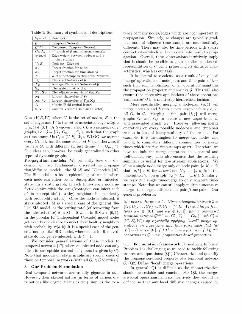
Table 1: Summary of symbols and descriptions

Symbol Description

G Temporal Network

Gcond Condensed Temporal Network

Gi, Ai ith graph of G and adjacency matrix

wi(a, b) Edge-weight between nodes a and bin time-stamp i

V ; E Node-set; Edge-set

αN Target fraction for nodes

αT Target fraction for time-stamps

T # of timestamps in Temporal Network

FG Flattened Network of GXG Average Flattened Network of GSG The system matrix of GFG ; XG The adjacency matrix of FG ; XGλS Largest eigenvalue of SGλF; λX Largest eigenvalue of FG ; XGA Matrix (Bold capital letter)

u, v Column Vectors (Bold small letter)

G = (V,E,W ) where V is the set of nodes, E is theset of edges and W is the set of associated edge-weightsw(a, b) ∈ [0, 1]. A temporal network G is a sequence of Tgraphs, i.e., G = {G1, G2, . . . , GT }, such that the graphat time-stamp i is Gi = (V,Ei,Wi). WLOG, we assumeevery Gi in G has the same node-set V (as otherwise, ifwe have Gi with different Vi, just define V = ∪Ti=1Vi).Our ideas can, however, be easily generalized to othertypes of dynamic graphs.Propagation models: We primarily base our dis-cussion on two fundamental discrete-time propaga-tion/diffusion models: the SI [3] and IC models [10].The SI model is a basic epidemiological model whereeach node can either be in ‘Susceptible’ or ‘Infected’state. In a static graph, at each time-step, a node in-fected/active with the virus/contagion can infect eachof its ‘susceptible’ (healthy) neighbors independentlywith probability w(a, b). Once the node is infected, itstays infected. SI is a special case of the general ‘flu-like’ SIS model, as the ‘curing rate’ (of recovering fromthe infected state) δ in SI is 0 while in SIS δ ∈ [0, 1).In the popular IC (Independent Cascade) model nodesget exactly one chance to infect their healthy neighborswith probability w(a, b); it is a special case of the gen-eral ‘mumps-like’ SIR model, where nodes in ‘Removed’state do not get re-infected, with δ = 1.

We consider generalizations of these models totemporal networks [17], where an infected node can onlyinfect its susceptible ‘current’ neighbors (as given by G).Note that models on static graphs are special cases ofthose on temporal networks (with all Gi ∈ G identical).

3 Our Problem Formulation

Real temporal networks are usually gigantic in size.However, their skewed nature (in terms of various dis-tributions like degree, triangles etc.) implies the exis-

tence of many nodes/edges which are not important inpropagation. Similarly, as changes are typically grad-ual, most of adjacent time-stamps are not drasticallydifferent. There may also be time-periods with sparseconnectivities which will not contribute much to prop-agation. Overall, these observations intuitively implythat it should be possible to get a smaller ‘condensed’representation of G while preserving its diffusive char-acteristics; which is our task.

It is natural to condense as a result of only local‘merge’ operations on node-pairs and time-pairs of G—such that each application of an operation maintainsthe propagation property and shrinks G. This will alsoensure that successive applications of these operations‘summarize’ G in a multi-step hierarchical fashion.

More specifically, merging a node-pair {a, b} willmerge nodes a and b into a new super-node say c, inall Gi in G. Merging a time-pair {i, j} will mergegraphs Gi and Gj to create a new super-time, k,and associated graph Gk. However, allowing mergeoperations on every possible node-pair and time-pairresults in loss of interpretability of the result. Forexample, it is meaningless to merge two nodes whobelong to completely different communities or mergetimes which are five time-stamps apart. Therefore, wehave to limit the merge operations in a natural andwell-defined way. This also ensures that the resultingsummary is useful for downstream applications. Weallow a single node-merge only on node pairs {a, b} suchthat {a, b} ∈ Ei for at least one Gi, i.e. {a, b} is in theunweighted ‘union graph’ UG(V,Eu = ∪iEi). Similarly,we restrict a single time-merge to only adjacent time-stamps. Note that we can still apply multiple successivemerges to merge multiple node-pairs/time-pairs. Ourgeneral problem is:

Informal Problem 1. Given a temporal network G ={G1, G2, . . . , GT } with Gi = (V,Ei,Wi) and target frac-tions αN ∈ (0, 1] and αT ∈ (0, 1], find a condensedtemporal network Gcond = {G′1, G′2, . . . , G′T ′} with G′i =(V ′, E′i,W

′i ) by repeatedly applying “local” merge op-

erations on node-pairs and time-pairs such that (a)|V ′| = (1− αN )|V |; (b) T ′ = (1− αT )T ; and (c) Gcond

approximates G w.r.t. propagation-based properties.

3.1 Formulation framework Formalizing InformalProblem 1 is challenging as we need to tackle followingtwo research questions: (Q1) Characterize and quantifythe propagation-based property of a temporal networkG; (Q2) Define “local” merge operations.

In general, Q1 is difficult as the characterizationshould be scalable and concise. For Q2, the mergesare local operations, and so intuitively they should bedefined so that any local diffusive changes caused by

them is minimum. Using Q1 and Q2, we can formulateInformal Problem 1 as an optimization problem wherethe search space is all possible temporal networks withthe desired size and which can be constructed via somesequence of repeated merges from G.

3.2 Q1: Propagation-based property One possi-ble naive answer is to run some diffusion model on Gand Gcond and see if the propagation is similar; but thisis too expensive. Therefore, we want to find a tractableconcise metric that can characterize and quantify prop-agation on a temporal network.

A major metric of interest in propagation on net-works is the epidemic threshold which indicates whetherthe virus/contagion will quickly spread throughout thenetwork (and cause an ‘epidemic’) or not, regardless ofthe initial conditions. Past works [6, 16] have stud-ied epidemic thresholds for various epidemic models onstatic graphs. Recently, [17] show that in context oftemporal networks and the SIS model, the thresholddepends on the largest eigenvalue λ of the so-called sys-tem matrix of G: an epidemic will not happen in G ifλ < 1. The result in [17] was only for undirected graphs;however it can be easily extended to weighted directedG with a strongly connected union graph UG (which justimplies that in principle any node can infect any othernode via a path, ignoring time; as otherwise we can justexamine each connected component separately).

Definition 1. System Matrix: For the SI model,the system matrix SG of a temporal network G ={G1, G2, ..., GT } is defined as SG =

∏Ti=1(I + Ai).

where At is the weighted adjacency matrix of Gt. Forthe SI model, the rate of infection is governed byλS, the largest eigenvalue of SG . Preserving λS whilecondensing G to Gcond will imply that the rate of virusspreading out in G and Gcond will be preserved too.Therefore λS is a well motivated and meaningful metricto preserve during condensation.

3.3 Q2: Merge Definitions We define two opera-tors: µ(G, i, j) merges a time-pair {i, j} in G to a super-time k in Gcond; while ζ(G, a, b) merges node-pair {a, b}in all Gi ∈ G and results in a super-node c in Gcond.

As stated earlier, we want to condense G by suc-cessive applications of µ and ζ. We also want themto preserve local changes in diffusion in the locality ofmerge operands. At the node level, the level where lo-cal merge operations are performed, the diffusion pro-cess is best characterized by the probability of infection.Hence, working from first principles, we design these op-erations to maintain the probabilities of infection beforeand after the merges in the ‘locality of change’ without

worrying about the system matrix. For µ(G, i, j), the‘locality of change’ is Gi, Gj and the new Gk. Whereas,for ζ(G, a, b), the ‘locality of change’ is the neighborhoodof {a, b} in all Gi ∈ G.Time-pair Merge: Consider a merge µ(G, i, j) be-tween consecutive times i and j. Consider any edge(a, b) in Gi and Gj (note if (a, b) /∈ Ei, then wi(a, b) = 0)and assume that node a is infected and node b is suscep-tible in Gi (illustrated in Figure 2 (a)). Now, node a caninfect node b in i via an edge in Gi, or in j via an edgein Gj . We want to maintain the local effects of propa-gation via the merged time-stamp Gk. Hence we needto readjust edge-weights in Gk such that it captures theprobability a infects b in G (in i and j).

Lemma 3.1. (Infection via i & j) Let Pr(a→ b|Gi, Gj)be the probability that a infects b in G in either time ior j, if it is infected in Gi. Then Pr(a → b|Gi, Gj) =[wi(a, b) + wj(a, b)], upto a first order approximation.

Lemma 3.1 suggests that the condensed time-stampk, after merging a time-pair {i, j} should be Ak =Ai + Aj . However, consider a G such that all Gi in Gare the same. This is effectively a static network: hencethe time-merges should give the network Gi rather thanTGi. This discrepancy arises because for any singletime-merge, as we reduce ‘T ’ from 2 to 1, to maintainthe final spread of the model, we have to increase theinfectivity along each edge by a factor of 2 (intuitivelyspeeding up the model [8]). Hence, the condensed

network at time k should be Ak =Ai+Aj

2 instead; whilefor the SI model, the rate of infection should be doubledfor time k in the system matrix. Motivated by theseconsiderations, we define a time-stamp merge as follows:

Definition 2. Time-Pair Merge µ(G, i, j). Themerge operator µ(G, i, j) returns a new time-stamp k

with weighted adjacency matrix Ak =Ai+Aj

2 .

Node-pair Merge: Similarly, in ζ(G, a, b) we need toadjust the weights of the edges to maintain the localeffects of diffusion between a and b and their neighbors.Note that when we merge two nodes, we need to mergethem in all Gi ∈ G.

Consider any time i. Suppose we merge {a, b} inGi to form super-node c in G′i (note that G′i ∈ Gcond).Consider a node x such that {a, b} and {a, x} areneighbors in Gi (illustrated in Figure 2 (b)). When c isinfected in G′i, it is intuitive to imply that either nodea or b is infected in Gi uniformly at random. Hencewe need to update the edge-weight from c to x in G′i,such that the new edge-weight is able to reflect theprobability that either node a or b infects x in Gi.

(a) Time merge of a single edge (b) Node Merge in a single time

Figure 2: (a) Example of merge operation on a single edge (a, b) when time-pair {i, j} is merged to form super-timek. (b) Example of node-pair {a, b} being merged in a single time i to form super-node c.

Lemma 3.2. (Probability of infecting out-neighbors) Ifeither node a or node b is infected in Gi and they aremerged to form a super-node c, then the first orderapproximation of probability of node c infecting its out-neighbors is given by:

Pr(c→ z|Gi) =

wi(a, z)

2∀z ∈ Nboi (a)\Nboi (b)

wi(b, z)

2∀z ∈ Nboi (b)\Nboi (a)

wi(a, z) + wi(b, z)

4∀z ∈ Nboi (a) ∩Nboi (b)

where, Nboi (v) is the set of out-neighbors of node v intime-stamp i. We can write down the correspondingprobability Pr(z → c|Gi) (for getting infected by in-neighbors) similarly. Motivated by Lemma 3.2, wedefine node-pair merge as:

Definition 3. Node-Pair merge ζ(G, a, b). Themerge operator ζ(G, a, b) merges a and b to form a newsuper-node c in all Gi ∈ G, s.t. wi(c, z) = Pr(c→ z|Gi)and wi(z, c) = Pr(z → c|Gi).

3.4 Problem Definition We can now formally de-fine our problem.

Problem 1. (Temporal Network CondensationProblem (TNC)) Given a temporal network G ={G1, G2, . . . , GT } with strongly connected UG, αN ∈(0, 1] and αT ∈ (0, 1], find a condensed temporal net-work Gcond = {G′1, G′2, . . . , G′T ′} with G′i = (V ′, E′i,W

′i )

by repeated applications of µ(G, ·, ·) and ζ(G, ·, ·), suchthat |V ′| = (1 − αN )|V |; T ′ = (1 − αT )T ; and Gcond

minimizes |λS − λcondS |.

Problem 1 naturally contains the GCP coarseningproblem for a static network [18] (which aims to preservethe largest eigenvalue of the adjacency matrix) as aspecial case: when G = {G}. GCP itself is a challengingproblem as it is related to immunization problems.Hence, Problem 1 is intuitively even more challenging.

4 Our Proposed Method

The naive algorithm is combinatorial. Even the greedymethod which computes the next best merge operands

(a) Temporal Network (b) Flattened NetworkFigure 3: (a) G, and (b) corresponding FG .

will be O(αN · V 6), even without time-pair merges. Infact, even computing SG is inherently non-trivial dueto matrix multiplications. It does not scale well forlarge temporal networks because SG gets denser as thenumber of time-stamps in G increases. Moreover, sinceSG is a dense matrix of size |V | by |V |, it does noteven fit in the main memory for large networks. Evenif there was an algorithm for Problem 1 that couldbypass computing SG , λS still has to be computed tomeasure success. Therefore, even just measuring successfor Problem 1, as is, seems hard.

4.1 Main idea To solve the numerical and computa-tional issues, our idea is to find an alternate representa-tion of G such that the new representation has the samediffusive properties and avoids the issues of SG . Thenwe develop an efficient sub-quadratic algorithm.

Our main idea is to look for a static network thatis similar to G with respect to propagation. We dothis in two steps. First we show how to construct astatic flattened network FG , and show that it has similardiffusive properties as G. We also show that eigenvaluesof SG and the adjacency matrix FG of FG are preciselyrelated. Due to this, computing eigenvalues of FG too isdifficult. Then in the second step, we derive a networkfrom FG whose largest eigenvalue is easier to computeand related to the largest eigenvalue of FG . Using it wepropose a new related problem, and solve it efficiently.

4.2 Step 1: An Alternate Static View Ourapproach for getting a static version is to expand Gand create layers of nodes, such that edges in G arecaptured by edges between the nodes in adjacent layers(see Figure 3). We call this the “flattened network” FG .

Definition 4. Flattened network. FG for G is de-fined as follows:

• Layers: FG consists of 1, ..., T layers correspond-ing to T time-stamps in G.

• Nodes: Each layer i has |V | nodes (so FG has T |V |nodes overall). Node a in the temporal network Gat time i is represented as ai in layer i of FG.

• Edges: At each layer i, each node ai has a directedge to a(i+1) mod T in layer (i + 1) mod T withedge-weight 1. And for each time-stamp Gi in thetemporal network G, if there is a directed edge (a, b),then in FG, we add a direct edge from node ai tonode b(i+1) mod T with weight wi(a, b).

For the relationship between G and FG , considerthe SI model running on G (Figure 3 (a)). Say node a isinfected in G1, which also means node a1 is infected inFG (Figure 3 (b)). Assume a infects b in G1. So in thebeginning of G2, a and b are infected. Correspondinglyin FG node a1 infects nodes a2 and b2. Now in G2, nofurther infection occurs. So the same nodes a and b areinfected in G3. However, in FG infection occurs betweenlayers 2 and 3, which means a2 infects a3 and b2 infectsb3. Propagation in FG is different than in G as each‘time-stamped’ node gets exactly one chance to infectothers. Note that the propagation model on FG we justdescribed is the popular IC model. Hence, running theSI model in G should be “equivalent” to running the ICmodel in FG in some sense.

We formalize this next. Assume we have the SImodel on G and the IC model on FG starting from thesame node-set of size I(0). Let IGSI(t) be the expectednumber of infected nodes at the end of time t. Similarly,let IFG

IC (T ) be the expected number of infected nodesunder the IC model till end of time T in FG . Note thatIFGIC (0) = IFG

SI (0) = I(0). Then:

Lemma 4.1. (Equivalence of propagation in G and FG)

We have∑Tt=1 I

GSI(t) = IFG

IC (T ).

That is, the cumulative expected infections for theSI model on G is the same as the infections after Tfor the IC model in FG . This suggests that the largesteigenvalues of SG and FG are closely related. Actually,we can prove a stronger statement that the spectra ofFG and G are closely related (Lemma 4.2).

Lemma 4.2. (Eigen-equivalence of SG and FG) Wehave (λF)T = λS. Furthermore, λ is an eigenvalue ofFG, iff λT is an eigenvalue of SG.

Lemma 4.2 implies that preserving λS in G isequivalent to preserving λF in FG . Therefore, Problem1 can be re-written in terms of λF (of a static network)instead of λS (of a temporal one).

4.3 Step 2: A Well Conditioned Network How-ever λF is problematic too. The difficulty in comput-ing λF arises because FG is ill-conditioned. So mod-ern packages take many iterations and the result maybe imprecise. Intuitively, it is easy to understand thatcomputing λF is difficult: as if it were not, computingλS itself would have been easy (just compute λF andraise it to the T -th power).

So we create a new static network that has a closerelation with FG and whose adjacency matrix is well-conditioned. To this end, we look at the average flat-tened network, XG , whose adjacency matrix is defined

as XG = FG+FG′

2 , where FG′ is the transpose of FG . It

is easy to see that trace of XG and FG are equal, whichmeans that the sum of eigenvalues of XG and FG areequal. Moreover, we have the following:

Lemma 4.3. (Eigenvalue relationship of FG and XG)The largest eigenvalue of FG, λF, and the largest eigen-value of XG, λX, are related as λF ≤ λX.

Note that if λX < 1, then λF < 1. Moreover, ifλF < 1 then λS < 1. Hence if there is no epidemicin XG , then there is no epidemic in FG as well, whichimplies that the rate of spread in G is low. Hence, XGis a good proxy static network for FG and G and λX is awell-motivated quantity to preserve. Also we need onlyweak-connectedness of UG for λX (and correspondingeigenvectors) to be real and positive (by the Perron-Frobenius theorem). Furthermore, XG is free of theproblems faced by FG and SG : it is well-conditionedand its eigenvalue can be efficiently computed.New problem: Considering all of the above, we re-formulate Problem 1 in terms of λX. Since G and XGare closely related networks, the merge definitions onXG can be easily extended from those on G.

Problem 2. Given G with weakly connected UG overV , αN and αT , find Gcond by repeated application ofµ(XG , ., .) and ζ(XG , ., .) such that |V ′| = (1 − αN )|V |;T ′ = (1− αT )T ; and Gcond minimizes |λX − λcond

X |.

4.4 NetCondense In this section, we propose a fastgreedy algorithm for Problem 2 called NetCondense,which only takes sub-quadratic time in the size of theinput. Again, the obvious approach is combinatorial.Consider a greedy approach using ∆-Score.

Definition 5. ∆-Score. ∆XG (a, b) = |λX − λcondX |

where λcondX is the largest eigenvalue of the new XG after

merging a and b (node or time-pair).

The greedy approach will successively choose thosemerge operands at each step which have the lowest

∆-Score. Doing this naively will lead to quartic time(due to repeated re-computations of λX for all possibletime/node-pairs). Recall that we limit time-merges toadjacent time-pairs and node-merges to node-pairs withan edge in UG . Now, computing ∆-Score simplyfor all edges (a, b) ∈ UG is still expensive. Hencewe estimate ∆-Score for node/time pairs instead usingMatrix Perturbation Theory [23]. Let u and v be rightand left eigenvector of XG , corresponding to λX. Letu(ai) and v(ai) be the right and left ‘eigenscore’ of nodeai in XG . Then we have the following lemmas.

Lemma 4.4. (∆-Score for time-pair) Let Vi = nodes inLayer i of XG. Now, for merge µ(XG , i, j) to form k,

∆XG (i, j) =−λX(

∑i∈Vi,Vj

η(i,i)) +∑

k∈Vkv(i)koTu + Y

vTu−∑

i∈Vi,Vjη(i,i)

upto a first-order approximation, where η(i,j) =u(i)v(j), Y =

∑i∈Vi,j∈Vj

(η(i,j) + η(j,i))XG(i, j), and

koTu = 12 (λXu(i) + λXu(j) + u(i) + u(j)).

Lemma 4.5. (∆-Score for node-pair) Let Va ={a1, a2, . . . , aT } ∈ XG corresponding to node a in G.For merge ζ(XG , a, b) to form c,

∆XG (a, b) =−λX(

∑a∈Va,Vb

η(a,a)) +∑

c∈Vcv(a)coTu + Y

vTu−∑

a∈Va,Vbη(a,a)

upto a first-order approximation, where η(a,b) =u(a)v(b), Y =

∑a∈Va,b∈Vb

(η(a,b) + η(b,a))XG(a, b), and

coTu = 12λX(u(a) + u(b)).

Our algorithm NetCondense works as follows: wefirst calculate ∆-Score for time-pairs based on Lemma4.4. Similarly, for all edges in UG using Lemma 4.5.Then we choose the top number of node/time-pairsbased on score, and we keep merging till Gcond is of thedesired size. Complete pseudo-code is in Algorithm 1.

Lemma 4.6. NetCondense has sub-quadratic time-complexity of O(TEu+E logE+αNθTV +αTE), whereθ is the maximum degree in any Gi ∈ G and linearspace-complexity of O(E + TV ).

Parallelizability: We can easily parallelize NetCon-dense: once the eigenvector of XG is computed, ∆-Score for node-pairs and time-pairs (loops in Lines 3and 5 in Algorithm 1) can be computed independent ofeach other in parallel. Similarly, µ and ζ operators (inLine 11) are also parallelizable.

5 Experiments

5.1 Experimental Setup We briefly describe ourset-up next. All experiments are conducted using a 4Xeon E7-4850 CPU with 512GB 1066Mhz RAM. Ourcode is publicly available for academic purposes1.

1http://people.cs.vt.edu/~bijaya/codes/NetCondense.zip

Algorithm 1 NetCondense

Require: Temporal graph G , 0 < αN < 1, 0 < αT < 1Ensure: Temporal graph Gcond(V ′, E′, T ′)1: obtain XG using Definition 4.2: for every adjacent time-pairs {i, j} do3: Calculate ∆XG (i, j) using Lemma 4.4

4: for every node-pair {a, b} in UG do5: Caluclate ∆XG (a, b) using Lemma 4.5

6: sort the lists of ∆-Score for time-pairs and node-pairs7: Gcond = G8: while |V ′| > αN · |V | or T ′ > αT · T do9: (x, y)← node-pair or time-pair with lowest ∆-Score

10: Gcond ← µ(Gcond, x, y) or ζ(Gcond, x, y)

11: return Gcond

Table 2: Datasets Information.

Dataset Weight |V | |E| T

WorkPlace Contact Hrs 92 1.5K 12 Days

School Contact Hrs 182 4.2K 9 Days

Enron # Emails 184 8.4K 44 Months

Chess # Games 7.3K 62.4K 9 Years

Arxiv # Papers 28K 3.8M 9 Years

Wikipedia # Pages 118K 2.1M 10 Years

WikiTalk # Messages 497K 2.7M 12 Years

DBLP # Papers 1.3M 18M 25 Years

Datasets. We run NetCondense on a variety of realdatasets (Table 2) of varying sizes from different do-mains such as social-interactions (WorkPlace, School,Chess), co-authorship (Arxiv, DBLP) and communi-cation (Enron, Wikipedia, WikiTalk). They includeweighted and both directed and undirected networks.Edge-weights are normalized to the range [0, 1].Baselines. Though there are no direct competitors, weadapt multiple methods to use as baselines.Random: Uniformly randomly choose node-pairs andtime-stamps to merge.Tensor: Here we pick merge operands based on thecentrality given by tensor decomposition. G can bealso seen as a tensor of size |V | × |V | × T . So werun PARAFAC decomposition [12] on G and choose thelargest component to get three vectors x, y, and z ofsize |V |, |V |, and T respectively. We compute pairwisecentrality measure for node-pair {a, b} as x(a) ·y(b) andfor time-pair {i, j} as z(i) · z(j) and choose the top-Kleast central ones.CNTemp: We run Coarsenet [18] (a summarizationmethod which preserves the diffusive property of a staticgraph) on UG and repeat the summary to create Gcond.

In Random and Tensor, we use our own mergedefinitions, hence the comparison is inherently unfair.

5.2 Perfomance of NetCondense: EffectivenessWe ran all the algorithms to get Gcond for differentvalues of αN and αT , and measure RX = λcond

X /λXto judge performance for Problem 2. See Figure 4.

NetCondense is able to preserve λX excellently (upto80% even when the the number of time-stamps andnodes are reduced by 50% and 70% respectively). Onthe other hand, the baselines perform much worse, andquickly degrade λX. Note that Tensor does not evenfinish within 7 days for DBLP for larger αN . Randomand Tensor perform poorly even though they use thesame merge definitions, showcasing the importance ofright merges. In case of Tensor, unexpectedly ittends to merge unimportant nodes with all nodes intheir neighborhood even if they are “important”; so itis unable to preserve λX. Finally CNTemp performsbadly as it does not use the full temporal nature of G.

(a) WikiTalk (b) DBLP

Figure 4: RX = λcondX /λX vs αN (top row, αT = 0.5)

and vs αT (bottom row, αN = 0.5).

We also compare our performance for Problem 1,against an algorithm specifically designed for it. We usethe simple greedy algorithm GreedySys for Problem 1(as the brute-force is too expensive): it greedily pickstop node/time merges by actually re-computing λS.We can run GreedySys only for small networks dueto the SG issues we mentioned before. See Figure 5(λM

S is λcondS obtained from method M). NetCondense

does almost as well as GreedySys, due to our carefultransformations and reductions.

(a) WorkPlace (b) School

Figure 5: Plot of RS = λNetCondenseS /λGreedySys

S .

5.3 Application 1: Temporal Influence Maxi-mization In this section, we show how to apply ourmethod to the well-known Influence Maximization prob-lem on a temporal network (TempInfMax) [2]. Given apropagation model, TempInfMax aims to find a seed-setS ⊆ V at time 0, which maximizes the ‘footprint’ (ex-pected number of infected nodes) at time T . Solving itdirectly on large G can be very slow. Here we proposeto use the much smaller Gcond as an approximation of G,as it maintains the propagation-based properties well.

Specifically, we propose CondInf (Algorithm 2) tosolve the TempInfMax problem on temporal networks.The idea is to get Gcond from NetCondense, solveTempInfMax problem on Gcond, and map the resultsback to G. Thanks to our well designed merging schemethat merges nodes with the similar diffusive propertytogether, a simple random mapping is enough. To bespecific, let the operator that maps node v from Gcond

to G be ζ−1(v). If v is a super-node then ζ−1(v) returnsa node sampled uniformly at random from v.

Algorithm 2 CondInf

Require: Temporal graph G , 0 < αN < 1, 0 < αT < 1Ensure: seed set S of top k seeds1: S = ∅2: Gcond ← NetCondense (G, αN , αT )3: k′1, k

′2, ..., k

′S ← Run base TempInfMax on Gcond

4: for every k′i do5: ki ← ζ−1(k′i); S ← S ∪ {ki}6: return S

We use two different base TempInfMax methods:ForwardInfluence [2] for the SI model and Greedy-OT [7] for the PersistentIC model. As our approachis general (our results can be easily extended to othermodels), and our actual algorithm/output is model-independent, we expect CondInf to perform well forboth these methods. To calculate the footprint, weinfect nodes in seed set S at time 0, and run theappropriate model till time T . We set αT = 0.5and αN = 0.5 for all datasets. We show results onlyfor ForwardInfluence in Table 3. The results forGreedy-OT were similar, however Greedy-OT didnot even finish for datasets larger than Enron. As wecan see, our method performs almost as good as the basemethod on G, while being significantly faster (upto 48times), showcasing its usefulness.

5.4 Application 2: Understanding/ExploringNetworks We can also use NetCondense for ‘sense-making’ of temporal datasets: it ensures that importantnodes and times remain unmerged while super-nodesand super-times form coherent interpretable groups ofnodes and time-stamps. This is not the case for thebaselines e.g. Tensor merges important nodes, giving

Table 3: Performance of CondInf (CI) with For-wardInfluence (FI) as base methods. σm and Tm arethe footprint and running time for method m respectively.‘-’ means the method did not finish.

Dataset σFI σCI TFI TCI

School 130 121 14s 3s

Enron 110 107 18s 3s

Chess 1293 1257 36m 45s

Arxiv 23768 23572 3.7d 7.5h

Wikipedia - 26335 - 7.1h

Figure 6: Condensed WorkPlace (αN = 0.6, αT = 0.5).

us heterogeneous super-nodes lacking interpretability.WorkPlace: It is a social-contact network betweenemployees of a company with five departments, whereweights are normalized contact time. In Gcond (seeFigure 6), we find a super-node composed mostly ofnodes from SRH (orange) and DSE (pink) departments,which were on floor 1 of the building while the rest wereon floor 2. In the same super-node, surprisingly, we finda node from DMCT (green) department on floor 2 whohas a high contact with DSE nodes. It turns out s/hewas labeled as a “wanderer” in [4].

Unmerged nodes in the Gcond had high degree inall T . For example, we found nodes 80, 150, 751,and 255 (colored black) remained unmerged even forαN = 0.9. In fact, all these nodes were classified as“Linkers” whose temporal stability is crucial for epi-demic spread [4]. The visualization of Gcond emphasizesthat linkers connect consistently to nodes from multipledepts.; which is not obvious in the original networks.We also examined the super-times, and discovered thatthe days in and around the weekend (where there is littleactivity) were merged together.School: It is socio-contact network between high schoolstudents from five different sections over several days [5].In Gcond, we find a super-node containing nodes fromMP*1 and MP*2 sections and another super-node withnodes from remaining three sections PC, PC*, and PSI.The groupings in the super-nodes are intuitive as thedataset can broadly be divided into two components(MP*1 and MP*2) and (PC, PC*, and PSI) [5].Enron: They are the email communication networks ofemployees of the Enron Corporation. In Gcond (αN =0.8, αT = 0.5), we find that unmerged nodes are im-portant nodes such as G. Whalley (President), K. Lay(CEO), and J. Skilling (CEO). We also found a star with

Chief of Staff S. Kean in the center and important offi-cials such as Whalley, Lay and J. Shankman (President)for six consecutive time-stamps. We also find a clique ofhigh ranking officials in the same period. These struc-tures appear only in consecutive time-stamps leading towhen Enron declared bankruptcy. Sudden emergence,stability for over six/seven time-stamps, and sudden dis-appearance of these structures correctly suggests that amajor event occurred during that time. We also notethat time-stamps in 2001 were never merged, indicativeof important and suspicious behavior.DBLP: These are co-authorship networks from DBLP-CSbibiliography. This is an especially large dataset: henceexploration without any condensation is hard. In Gcond

(αN = 0.7, αT = 0.5), we found that the unmergednodes were very well-known researchers such as PhilipS. Yu, Christos Faloutsos, Rakesh Aggarwal, and soon.We also find a giant super-node of size 395, 000.An interesting observation is that famous researchersconnect very weakly to the giant super-node. Whereas,less known researchers connect to the giant super-nodewith higher edge-weights. Another common patternamong famous researchers is that they connect to super-nodes only in the earlier time-stamps in the dataset.This observation suggests that as the authors becomemore famous, they collaborate less with non-famousresearchers or their collaborators too become famous.

(a) Scalability (b) ParallelizabilityFigure 7: Near-linear running time and speed-up.

5.5 Scalability and Parallelizability Figure 7 (a)shows the runtime of NetCondense on the compo-nents of increasing size of Arxiv. NetCondense hassubquadratic time complexity. In practice, it is near-linear w.r.t input size. Figure 7 (b) shows the near-linear run-time speed-up of parallel-NetCondense vs# cores on Wikipedia.

6 Related Work

Mining Dynamic Graphs. Dynamic graphs havegained a lot of interest recently (see [1] for a survey).Many graph mining tasks on static graphs have beenintroduced to dynamic graphs, including communitydetection [24] and link prediction [21]. Due to theincreasing size, typically it is challenging to performanalysis on temporal networks.Propagation. Cascade processes have been widelystudied, including in epidemiology [3, 8], information

diffusion [10], cyber-security [11] and product market-ing [20]. A lot of work has been done on determiningthe epidemic threshold i.e. the conditions under whicha virus causes an epidemic [6, 16, 17]. Examples ofpropagation-based optimization problems are influencemaximization [10, 7, 2], and immunization [26]. Re-motely related work deals with weak and strong tiesover time for diffusion [9].Graph Summarization. Here, we seek to find a com-pact representation of a large graph by leveraging globaland local graph properties like local neighborhood struc-ture [15], node/edge attributes [25], action logs [19],eigenvalue of the adjacency matrix [18], and key sub-graphs. It is also related to graph sparsification algo-rithms [14]. The goal is to either reduce storage andmanipulation costs, or simplify structure. Summariz-ing temporal networks has not seen much work, exceptrecent papers based on bits-storage-compression [13],or extracting a list of recurrent sub-structures overtime [22]. Unlike these, we are the first to focus on hier-archical condensation: using structural merges, giving asmaller propagation-equivalent temporal network.

7 Discussion and Conclusions

In this paper, we proposed a novel general TemporalNetwork Condensation Problem using the funda-mental so-called ‘system matrix’ and present an effec-tive, near-linear and parallelizable algorithm NetCon-dense. Using a variety of large datasets, we leverageit to dramatically speed-up influence maximization al-gorithms on temporal networks, and to explore and un-derstand complex datasets. As also shown by our ex-periments, it is useful to note that our method itselfis model-agnostic and has wide-applicability, thanks toour carefully chosen metrics which can be easily gener-alized to other propagation models. There are multipleideas to explore: including leveraging NetCondensefor other tasks such as role discovery and immunization.Acknowledgements This paper is based on work partially

supported by the NSF (IIS-1353346), the NEH (HG-229283-

15), ORNL (Task Order 4000143330) and from the Maryland

Procurement Office (H98230-14-C- 0127), and a Facebook

faculty gift.References

[1] C. Aggarwal and K. Subbian. Evolutionary networkanalysis: A survey. ACM Computing Survey, 2014.

[2] C. C. Aggarwal, S. Lin, and S. Y. Philip. On influentialnode discovery in dynamic social networks. In SDM,2012.

[3] R. M. Anderson and R. M. May. Infectious Diseasesof Humans. Oxford University Press, 1991.

[4] M. G. et. al. Data on face-to-face contacts in an officebuilding suggest a low-cost vaccination strategy basedon community linkers. Network Science, 3(03), 2015.

[5] J. Fournet and A. Barrat. Contact patterns amonghigh school students. PloS one, 9(9):e107878, 2014.

[6] A. Ganesh, L. Massoulie, and D. Towsley. The effectof network topology in spread of epidemics. IEEEINFOCOM, 2005.

[7] N. T. Gayraud, E. Pitoura, and P. Tsaparas. Diffusionmaximization in evolving social networks. In COSN,2015.

[8] H. W. Hethcote. The mathematics of infectious dis-eases. SIAM review, 42(4):599–653, 2000.

[9] M. Karsai, N. Perra, and A. Vespignani. Time varyingnetworks and the weakness of strong ties. ScientificReports, 4:4001, 2014.

[10] D. Kempe, J. Kleinberg, and E. Tardos. Maximizingthe spread of influence through a social network. InKDD, 2003.

[11] J. O. Kephart and S. R. White. Measuring andmodeling computer virus prevalence. In Research inSecurity and Privacy, pages 2–15. IEEE, 1993.

[12] T. G. Kolda and B. W. Bader. Tensor decompositionsand applications. SIAM Review, 51(3):455–500, 2009.

[13] W. Liu, A. Kan, J. Chan, J. Bailey, C. Leckie, J. Pei,and R. Kotagiri. On compressing weighted time-evolving graphs. In CIKM12. ACM, 2012.

[14] M. Mathioudakis, F. Bonchi, C. Castillo, A. Gionis,and A. Ukkonen. Sparsification of influence networks.In KDD, pages 529–537. ACM, 2011.

[15] S. Navlakha, R. Rastogi, and N. Shrivastava. Graphsummarization with bounded error. In SIGMOD, 2008.

[16] B. A. Prakash, D. Chakrabarti, M. Faloutsos, N. Valler,and C. Faloutsos. Threshold conditions for arbitrarycascade models on arbitrary networks. In ICDM, 2011.

[17] B. A. Prakash, H. Tong, N. Valler, M. Faloutsos,and C. Faloutsos. Virus propagation on time-varyingnetworks: Theory and immunization algorithms. InECML/PKDD10, 2010.

[18] M. Purohit, B. A. Prakash, C. Kang, Y. Zhang, andV. Subrahmanian. Fast influence-based coarsening forlarge networks. In KDD14.

[19] Q. Qu, S. Liu, C. S. Jensen, F. Zhu, and C. Faloutsos.Interestingness-driven diffusion process summarizationin dynamic networks. In ECML/PKDD. 2014.

[20] E. M. Rogers. Diffusion of innovations. 2010.[21] P. Sarkar, D. Chakrabarti, and M. Jordan. Nonpara-

metric link prediction in dynamic networks. In ICML,2012.

[22] N. Shah, D. Koutra, T. Zou, B. Gallagher, andC. Faloutsos. Timecrunch: Interpretable dynamicgraph summarization. In KDD15.

[23] G. W. Stewart. Matrix perturbation theory. 1990.[24] C. Tantipathananandh and T. Y. Berger-Wolf. Finding

communities in dynamic social networks. In ICDM11.[25] N. Zhang, Y. Tian, and J. M. Patel. Discovery-driven

graph summarization. In ICDE, 2010.[26] Y. Zhang and B. A. Prakash. Dava: Distributing

vaccines over networks under prior information. InSDM, 2014.