Confidence intervals, t tests, P values
42
Confidence intervals, t tests, P values Joe Felsenstein Department of Genome Sciences and Department of Biology Confidence intervals, t tests, P values – p.1/31
Transcript of Confidence intervals, t tests, P values

Confidence intervals, t tests, P values
Joe Felsenstein
Department of Genome Sciences and Department of Biology
Confidence intervals,t tests,P values – p.1/31
Normality
Everybody believes in the normal approximation, the experimentersbecause they think it is a mathematical theorem, the mathematiciansbecause they think it is an experimental fact! G. Lippman
We can use the Gaussian (normal) distribution, assumed correct,and estimate the mean (which is the expectation). It turns out that,not surprisingly, the best estimate of the mean is the mean of thesample.
Confidence intervals,t tests,P values – p.2/31
Normality
Everybody believes in the normal approximation, the experimentersbecause they think it is a mathematical theorem, the mathematiciansbecause they think it is an experimental fact! G. Lippman
We can use the Gaussian (normal) distribution, assumed correct,and estimate the mean (which is the expectation). It turns out that,not surprisingly, the best estimate of the mean is the mean of thesample.
(The median of the sample is a legitimate estimate too, but it isnoisier).
The sample mean is the optimal estimate as it is the MaximumLikelihood Estimate – for which see later in the course.
Confidence intervals,t tests,P values – p.2/31
Normality
Everybody believes in the normal approximation, the experimentersbecause they think it is a mathematical theorem, the mathematiciansbecause they think it is an experimental fact! G. Lippman
We can use the Gaussian (normal) distribution, assumed correct,and estimate the mean (which is the expectation). It turns out that,not surprisingly, the best estimate of the mean is the mean of thesample.
(The median of the sample is a legitimate estimate too, but it isnoisier).
The sample mean is the optimal estimate as it is the MaximumLikelihood Estimate – for which see later in the course.But how do we figure out how noisy the estimate is?
Can we make an interval estimate?
Confidence intervals,t tests,P values – p.2/31
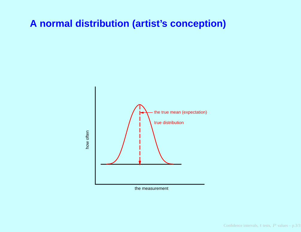
A normal distribution (artist’s conception)
true distribution
how
ofte
n
the measurement
the true mean (expectation)
Confidence intervals,t tests,P values – p.3/31
Uncertainty of the mean
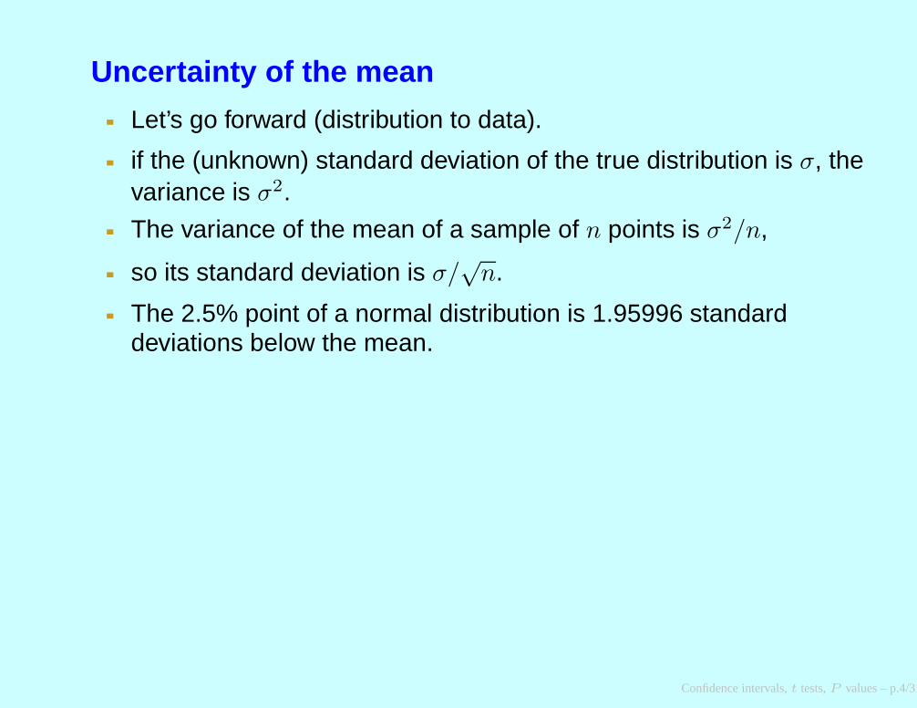
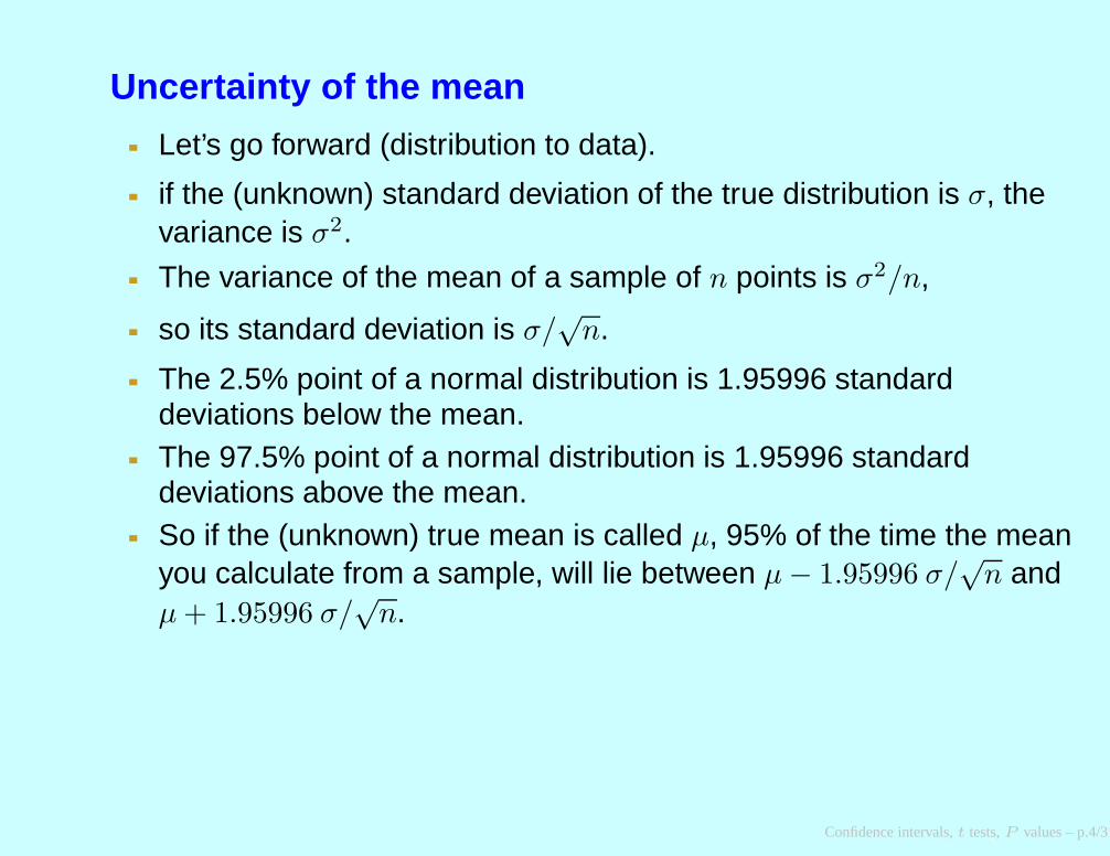
Let’s go forward (distribution to data).
Confidence intervals,t tests,P values – p.4/31
Uncertainty of the mean
Let’s go forward (distribution to data).
if the (unknown) standard deviation of the true distribution is σ, thevariance is σ2.
Confidence intervals,t tests,P values – p.4/31
Uncertainty of the mean
Let’s go forward (distribution to data).
if the (unknown) standard deviation of the true distribution is σ, thevariance is σ2.
The variance of the mean of a sample of n points is σ2/n,
Confidence intervals,t tests,P values – p.4/31
Uncertainty of the mean
Let’s go forward (distribution to data).
if the (unknown) standard deviation of the true distribution is σ, thevariance is σ2.
The variance of the mean of a sample of n points is σ2/n,
so its standard deviation is σ/√
n.
Confidence intervals,t tests,P values – p.4/31
Uncertainty of the mean
Let’s go forward (distribution to data).
if the (unknown) standard deviation of the true distribution is σ, thevariance is σ2.
The variance of the mean of a sample of n points is σ2/n,
so its standard deviation is σ/√
n.
The 2.5% point of a normal distribution is 1.95996 standarddeviations below the mean.
Confidence intervals,t tests,P values – p.4/31

Uncertainty of the mean
Let’s go forward (distribution to data).
if the (unknown) standard deviation of the true distribution is σ, thevariance is σ2.
The variance of the mean of a sample of n points is σ2/n,
so its standard deviation is σ/√
n.
The 2.5% point of a normal distribution is 1.95996 standarddeviations below the mean.The 97.5% point of a normal distribution is 1.95996 standarddeviations above the mean.
Confidence intervals,t tests,P values – p.4/31
Uncertainty of the mean
Let’s go forward (distribution to data).
if the (unknown) standard deviation of the true distribution is σ, thevariance is σ2.
The variance of the mean of a sample of n points is σ2/n,
so its standard deviation is σ/√
n.
The 2.5% point of a normal distribution is 1.95996 standarddeviations below the mean.The 97.5% point of a normal distribution is 1.95996 standarddeviations above the mean.So if the (unknown) true mean is called µ, 95% of the time the meanyou calculate from a sample, will lie between µ − 1.95996 σ/
√
n andµ + 1.95996 σ/
√
n.
Confidence intervals,t tests,P values – p.4/31
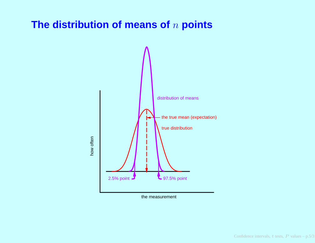
The distribution of means of n points
how
ofte
n
the measurement
the true mean (expectation)
true distribution
distribution of means
2.5% point 97.5% point
Confidence intervals,t tests,P values – p.5/31
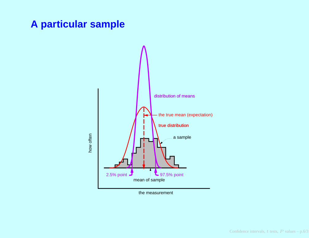
A particular sample
true distribution
mean of sample
distribution of means
a sample
how
ofte
n
the measurement
the true mean (expectation)
true distribution
distribution of means
2.5% point 97.5% point
Confidence intervals,t tests,P values – p.6/31
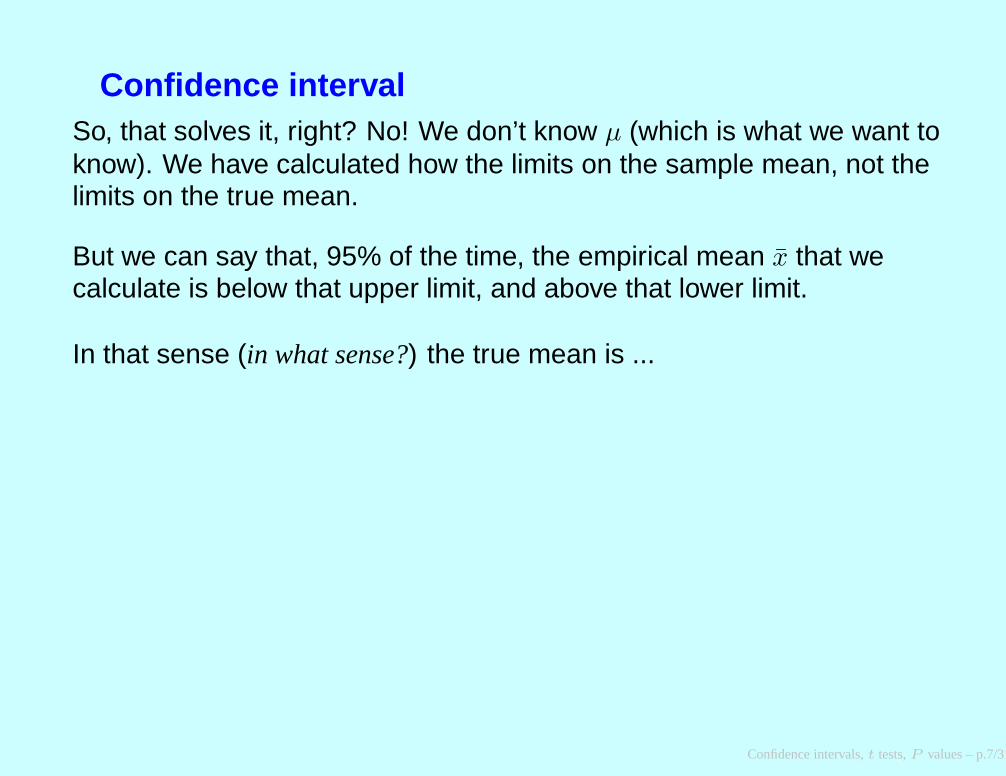
Confidence intervalSo, that solves it, right? No! We don’t know µ (which is what we want toknow). We have calculated how the limits on the sample mean, not thelimits on the true mean.
But we can say that, 95% of the time, the empirical mean x that wecalculate is below that upper limit, and above that lower limit.
In that sense (in what sense?) the true mean is ...
Confidence intervals,t tests,P values – p.7/31
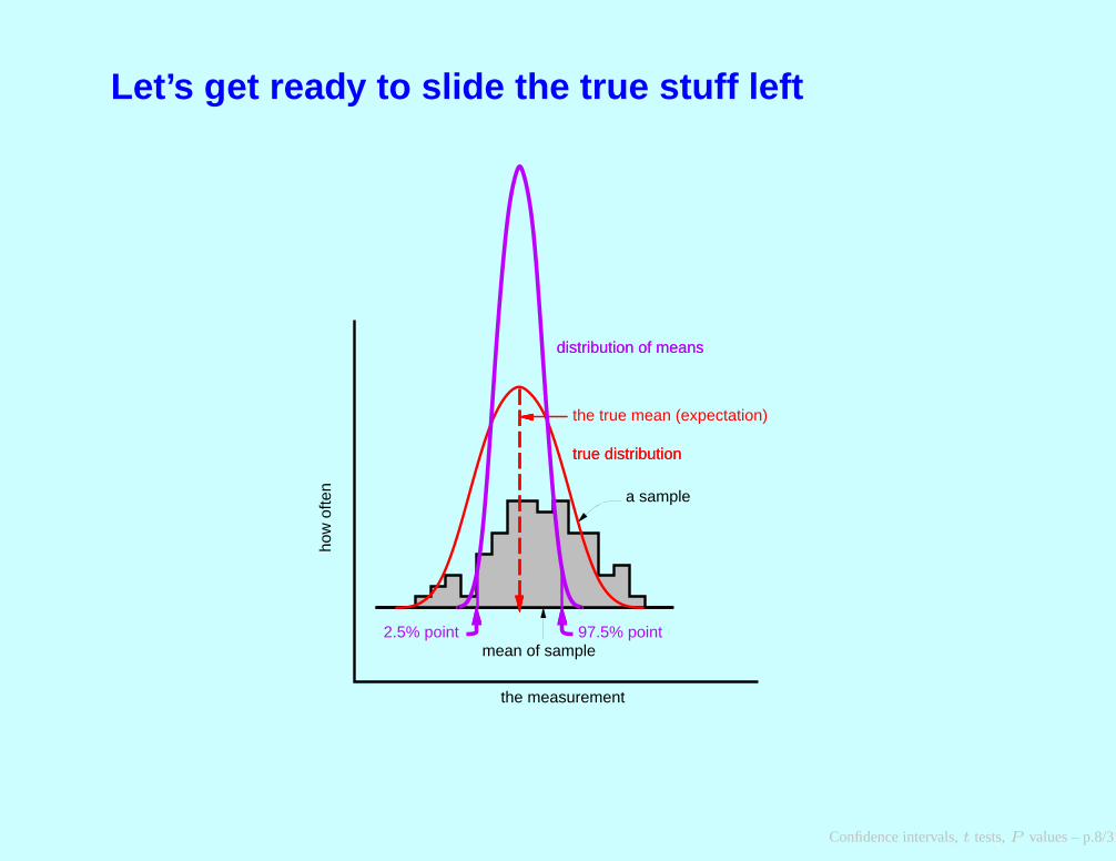
Let’s get ready to slide the true stuff left
true distribution
mean of sample
distribution of means
a sample
how
ofte
n
the measurement
the true mean (expectation)
true distribution
distribution of means
2.5% point 97.5% point
Confidence intervals,t tests,P values – p.8/31
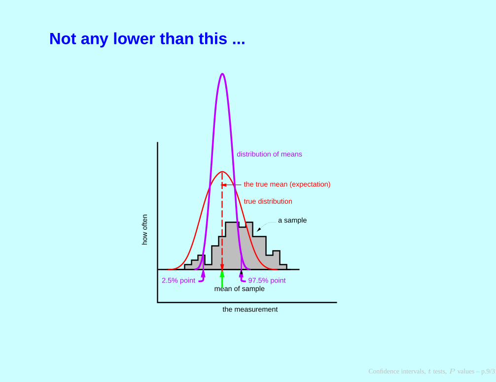
Not any lower than this ...
mean of sample
a sample
how
ofte
n
the measurement
distribution of means
the true mean (expectation)
2.5% point 97.5% point
true distribution
Confidence intervals,t tests,P values – p.9/31
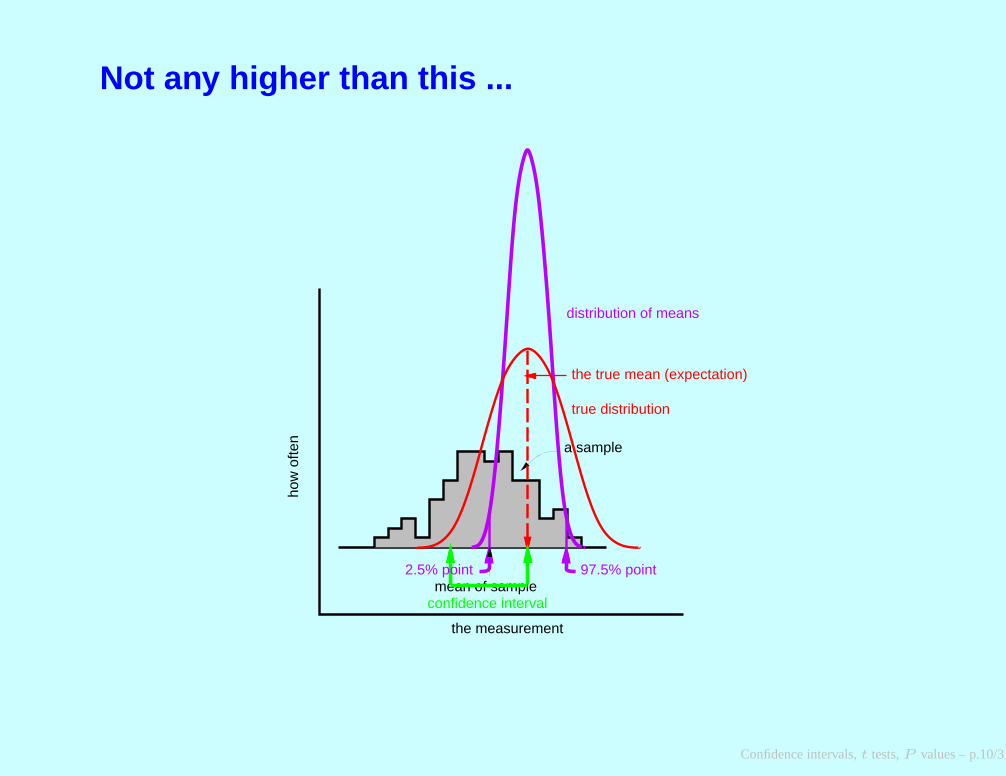
Not any higher than this ...
mean of sample
a sample
how
ofte
n
the measurement
distribution of means
confidence interval
the true mean (expectation)
2.5% point 97.5% point
true distribution
Confidence intervals,t tests,P values – p.10/31
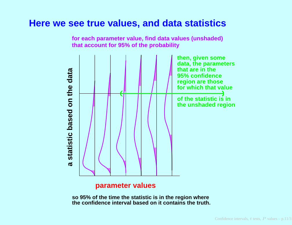
Here we see true values, and data statisticsfor each parameter value, find data values (unshaded)that account for 95% of the probability
a st
atis
tic b
ased
on
the
data
parameter values
then, given somedata, the parametersthat are in the95% confidenceregion are thosefor which that value
so 95% of the time the statistic is in the region wherethe confidence interval based on it contains the truth.
of the statistic is inthe unshaded region
Confidence intervals,t tests,P values – p.11/31
In what sense??You could say that if you do this throughout your career, 95% of theseintervals will contain the true value.
This is fairly unsatisfactory, as it acts as if the outcome of someother, unrelated, experiment is relevant.
Confidence intervals,t tests,P values – p.12/31
In what sense??You could say that if you do this throughout your career, 95% of theseintervals will contain the true value.
This is fairly unsatisfactory, as it acts as if the outcome of someother, unrelated, experiment is relevant.
Maybe best this way: if you did this experiment again and again andagain, each time making a confidence interval for the mean, 95% ofthose intervals would contain the true value.
Confidence intervals,t tests,P values – p.12/31
The Bayesian alternative
We will cover this later (lecture 6). It involves assuming that we know aprior probability of the parameters (in this case of the mean µ of the truedistribution and the standard deviation σ).
Then, using Bayes’ Formula (which we see in that lecture) we cancompute the posterior probability of the parameter, given the data.
This gives us what we really wanted: the probabilities (or probabilitydensities) of different values of the parameters. But it is achieved at thecost of having to have a prior distribution for them that we are assuming istrue.
The present approach instead makes a different assumption, that we canregard the experiment as a repeatable trial. This Frequentist approachand the Bayesian approach both have supporters among statisticians –the issue is one’s philosophy of science, not a technical disagreementabout statistics.
Confidence intervals,t tests,P values – p.13/31
Coping with not knowing the standard deviation
So far we have casually assumed we know the standard deviation σ of the true distribution.
But generally we don’t. The upper (lower) 2.5% point of the sample means is 1.95996 σ. But
if we look at the estimate of σ2, its unbiased estimate is (for reasons connected with also
estimating the mean)
s2 =
nP
i=1
(xi − x)2
n − 1
(the n − 1 instead of n is to correct for xi being a bit closer tox than it should be, because xi is part of x as well).
The standard deviation we use is the (estimated) standarddeviation of the mean, which is s/
√
n.
The quantity 1.95996 needs to be replaced by something thatcorrects for us sometimes having a s that is smaller than σ,and sometimes larger.
Here’s why, in this case “Guiness is good for you”:
Confidence intervals,t tests,P values – p.14/31
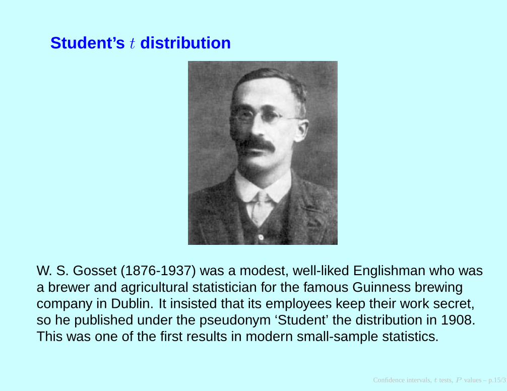
Student’s t distribution
W. S. Gosset (1876-1937) was a modest, well-liked Englishman who wasa brewer and agricultural statistician for the famous Guinness brewingcompany in Dublin. It insisted that its employees keep their work secret,so he published under the pseudonym ‘Student’ the distribution in 1908.This was one of the first results in modern small-sample statistics.
Confidence intervals,t tests,P values – p.15/31
Why we have to make the confidence interval wider
We can’t just say that the estimated σ is sometimes 20% smaller than thetrue value, and sometimes 20% larger, so it all cancels out.
It doesn’t, because σ doesn’t have a symmetrical distribution, butsomething derived from a chi-square distribution (which we have notintroduced yet).
Confidence intervals,t tests,P values – p.16/31
The t statisticThis is the number of (estimated) standard deviations of the mean that themean deviates from its expected value.
If s is the estimated standard deviation, from a sample of n values, andthe mean of the sample is x , while the expectation of that mean is µ, then
t =x − µ
s/√
n
This does not have a normal distribution but it is closer to normal thebigger n is. The quantity n − 1 is called the degrees of freedomof the t
value.
Confidence intervals,t tests,P values – p.17/31
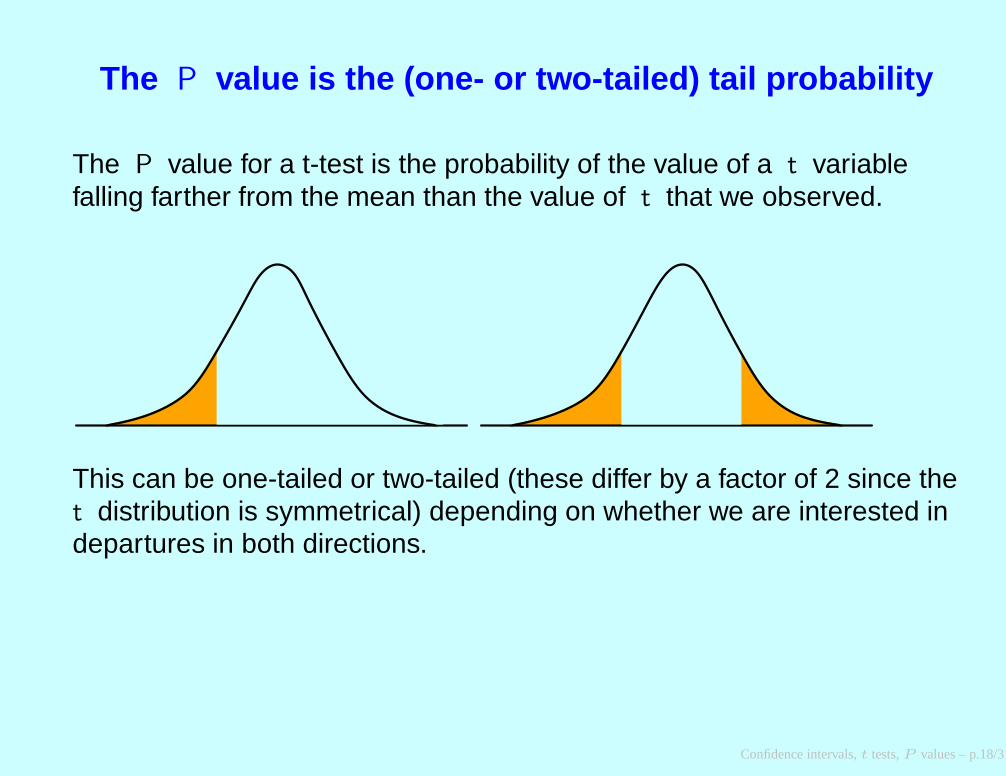
The P value is the (one- or two-tailed) tail probability
The P value for a t-test is the probability of the value of a t variablefalling farther from the mean than the value of t that we observed.
This can be one-tailed or two-tailed (these differ by a factor of 2 since thet distribution is symmetrical) depending on whether we are interested indepartures in both directions.
Confidence intervals,t tests,P values – p.18/31
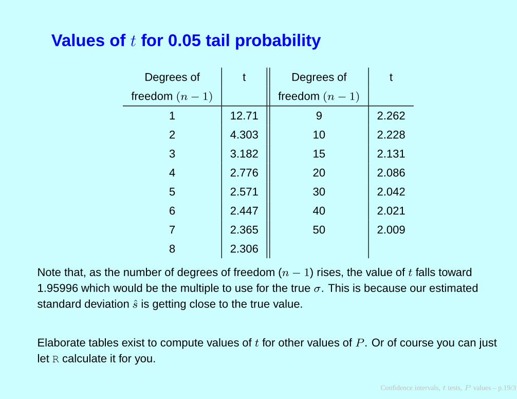
Values of t for 0.05 tail probability
Degrees of t Degrees of t
freedom (n − 1) freedom (n − 1)
1 12.71 9 2.262
2 4.303 10 2.228
3 3.182 15 2.131
4 2.776 20 2.086
5 2.571 30 2.042
6 2.447 40 2.021
7 2.365 50 2.009
8 2.306
Note that, as the number of degrees of freedom (n − 1) rises, the value of t falls toward1.95996 which would be the multiple to use for the true σ. This is because our estimatedstandard deviation s is getting close to the true value.
Elaborate tables exist to compute values of t for other values of P . Or of course you can justlet R calculate it for you.
Confidence intervals,t tests,P values – p.19/31
Why 0.05?
No real reason.
It is mostly an historical accident of the values R. A. Fisher chose to use inhis incredibly influential 1922 book Statistical Methods for Research Workers.
The more cautious you need to be the smaller tail probability P you shouldchoose. (Note: sometimes people describe the non-tail probability, suchas 95%, instead).
Confidence intervals,t tests,P values – p.20/31
Statistical tests and confidence intervalsIf someone suggests that the true µ is (say) 3.14159, we can test this byseeing whether 3.14159 is within the confidence interval. If it isn’t, wereject that hypothesis (the null hypothesis).
Alternatively, we can calculate for what value of P the suggested value(3.14159 in this case) is just within the confidence interval. We might get,for example, 0.09. That means it is within the interval calculated for amore extreme tail probability 0.05, Departure of the mean from 3.14159 isnot significant. We can report the 0.09 to indicate to the reader how closeto significance it was.
Getting all worried about whether 0.09 is “significantly larger than 0.05” isnot worth it. If we think about the “significance of the significance”, thatway lies madness!
The 0.05 is the “type I error” of the test. It is the fraction of the time (whenthe null hypothesis is true) that we get a “false positive” and reject it.
Confidence intervals,t tests,P values – p.21/31
One-tailed testIf we just want to know whether our mean is significantly bigger than3.14159, but do not want to get excited if it is smaller, we do a one-tailed ttest. We get the tail probability of 0.05 on one side, and 0.05 on the other(before we used 0.025 on each). Then we ignore the uninteresting tail (inthis case the upper tail – think about it ...)
This will make sense, for example, if we want to get excited about a drugand develop it further if it causes us to lose weight, but not if it causes usto gain weight.
Confidence intervals,t tests,P values – p.22/31
Paired two-sample t-test
Suppose we have two samples of the same size (say 25 numbers) andthe corresponding numbers pair naturally. That is, there are some sourcesof error (“noise”) that are shared by both members of a pair. For example,we might do before-and-after pairs of measurements after giving a drug.Or measure gene expression levels of a gene on two samples (oneEuropean and one African) on the same day, and do pairs of indviduals,one from each continent, on 25 different days.
The difference between two independent normally-distributed quantities isitself normally distributed. So to measure whether the “after” member ofthe pair is different from the “before” member, we just subtract them, andtest whether the mean of this sample of differences is 0. It is then just aone-sample t test of the sort we used above. The standard deviation youuse is the standard deviation of the differences, not of the individualmembers of the pair.
If the shared noise is large, this can be incredibly more appropriate thanthe next test ...
Confidence intervals,t tests,P values – p.23/31
(Unpaired) two-sample t test
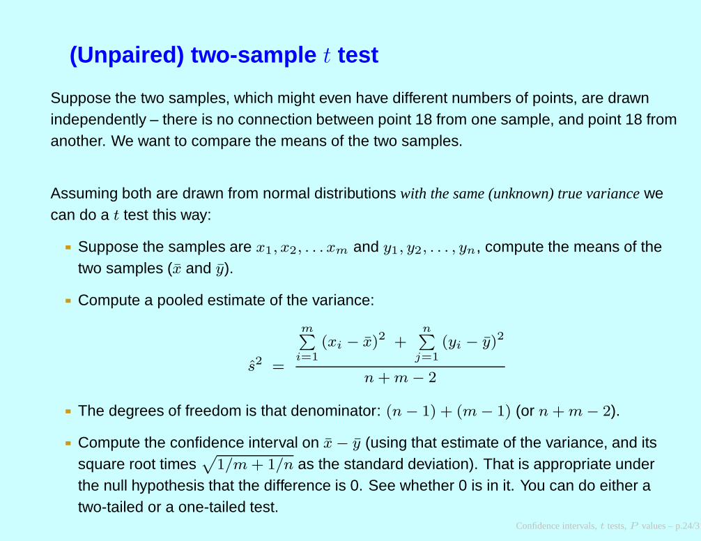
Suppose the two samples, which might even have different numbers of points, are drawnindependently – there is no connection between point 18 from one sample, and point 18 fromanother. We want to compare the means of the two samples.
Assuming both are drawn from normal distributions with the same (unknown) true variancewecan do a t test this way:
Suppose the samples are x1, x2, . . . xm and y1, y2, . . . , yn, compute the means of thetwo samples (x and y).
Compute a pooled estimate of the variance:
s2 =
mP
i=1
(xi − x)2 +n
P
j=1
(yi − y)2
n + m − 2
The degrees of freedom is that denominator: (n − 1) + (m − 1) (or n + m − 2).
Compute the confidence interval on x − y (using that estimate of the variance, and itssquare root times
p
1/m + 1/n as the standard deviation). That is appropriate underthe null hypothesis that the difference is 0. See whether 0 is in it. You can do either atwo-tailed or a one-tailed test.
Confidence intervals,t tests,P values – p.24/31
Gene expression levels in two individuals
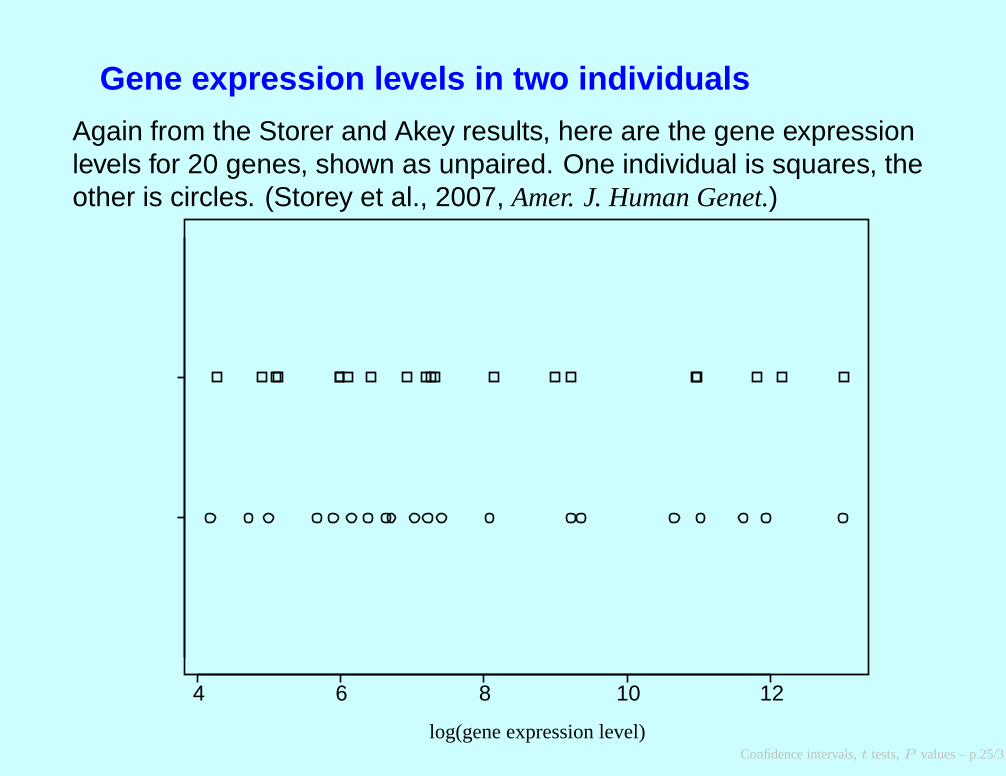
Again from the Storer and Akey results, here are the gene expressionlevels for 20 genes, shown as unpaired. One individual is squares, theother is circles. (Storey et al., 2007, Amer. J. Human Genet.)
4 6 8 10 12
log(gene expression level)Confidence intervals,t tests,P values – p.25/31
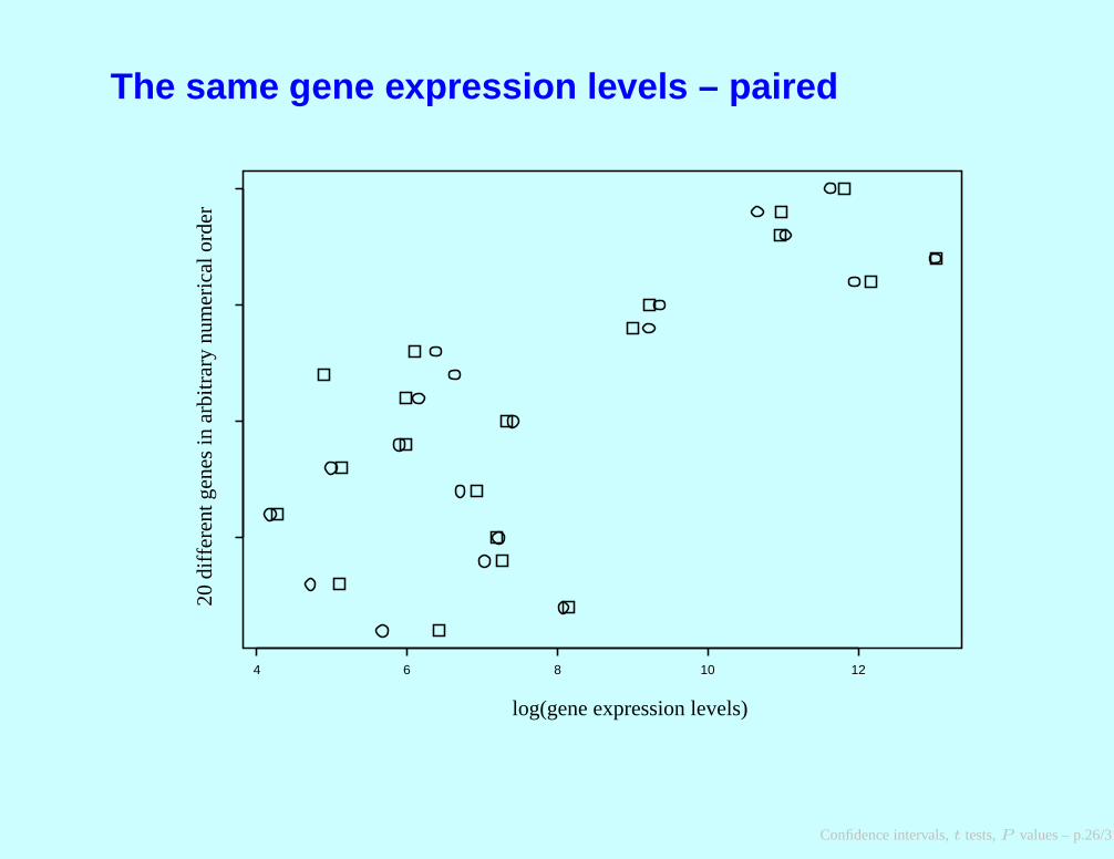
The same gene expression levels – paired
4 6 8 10 12
log(gene expression levels)
20 d
iffer
ent g
enes
in a
rbitr
ary
num
eric
al o
rder
Confidence intervals,t tests,P values – p.26/31
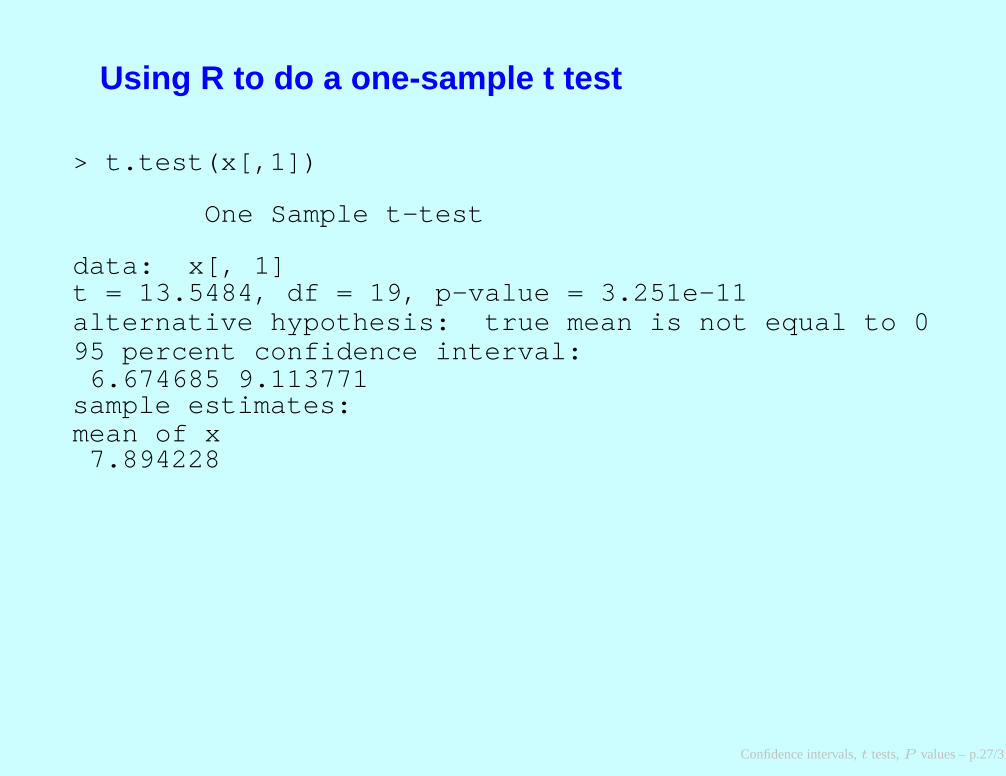
Using R to do a one-sample t test
> t.test(x[,1])
One Sample t-test
data: x[, 1]t = 13.5484, df = 19, p-value = 3.251e-11alternative hypothesis: true mean is not equal to 095 percent confidence interval:6.674685 9.113771sample estimates:mean of x7.894228
Confidence intervals,t tests,P values – p.27/31
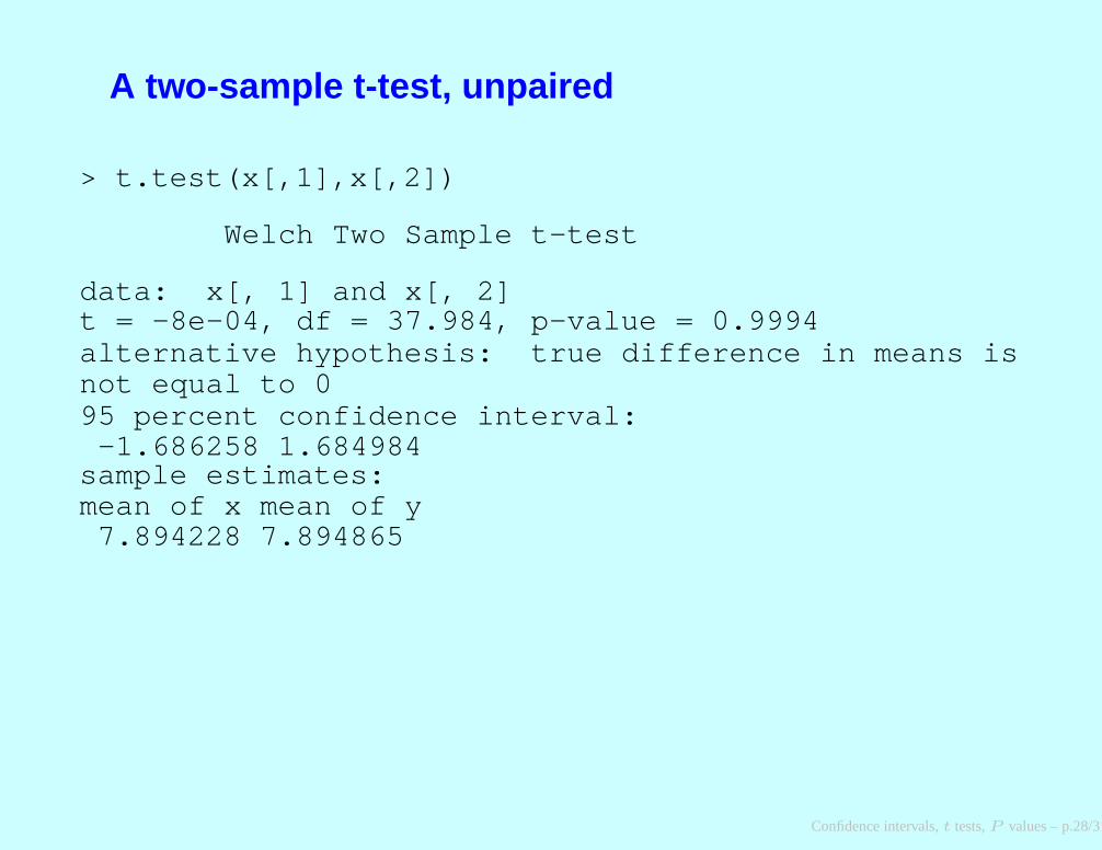
A two-sample t-test, unpaired
> t.test(x[,1],x[,2])
Welch Two Sample t-test
data: x[, 1] and x[, 2]t = -8e-04, df = 37.984, p-value = 0.9994alternative hypothesis: true difference in means isnot equal to 095 percent confidence interval:-1.686258 1.684984sample estimates:mean of x mean of y7.894228 7.894865
Confidence intervals,t tests,P values – p.28/31
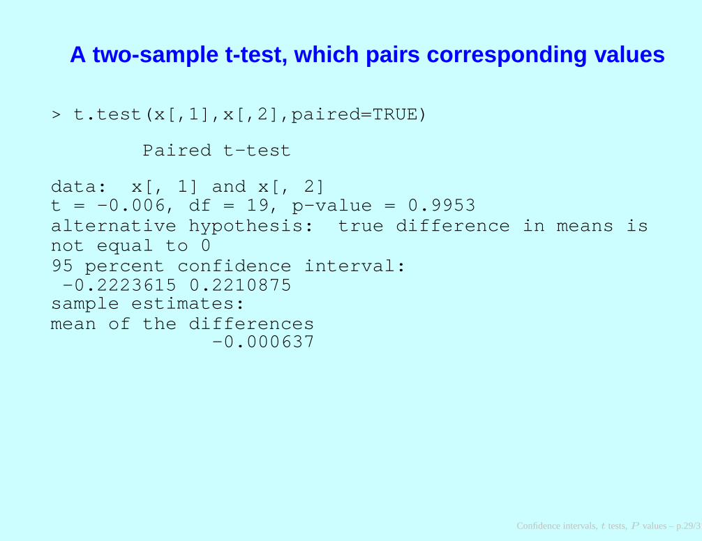
A two-sample t-test, which pairs corresponding values
> t.test(x[,1],x[,2],paired=TRUE)
Paired t-test
data: x[, 1] and x[, 2]t = -0.006, df = 19, p-value = 0.9953alternative hypothesis: true difference in means isnot equal to 095 percent confidence interval:-0.2223615 0.2210875sample estimates:mean of the differences
-0.000637
Confidence intervals,t tests,P values – p.29/31
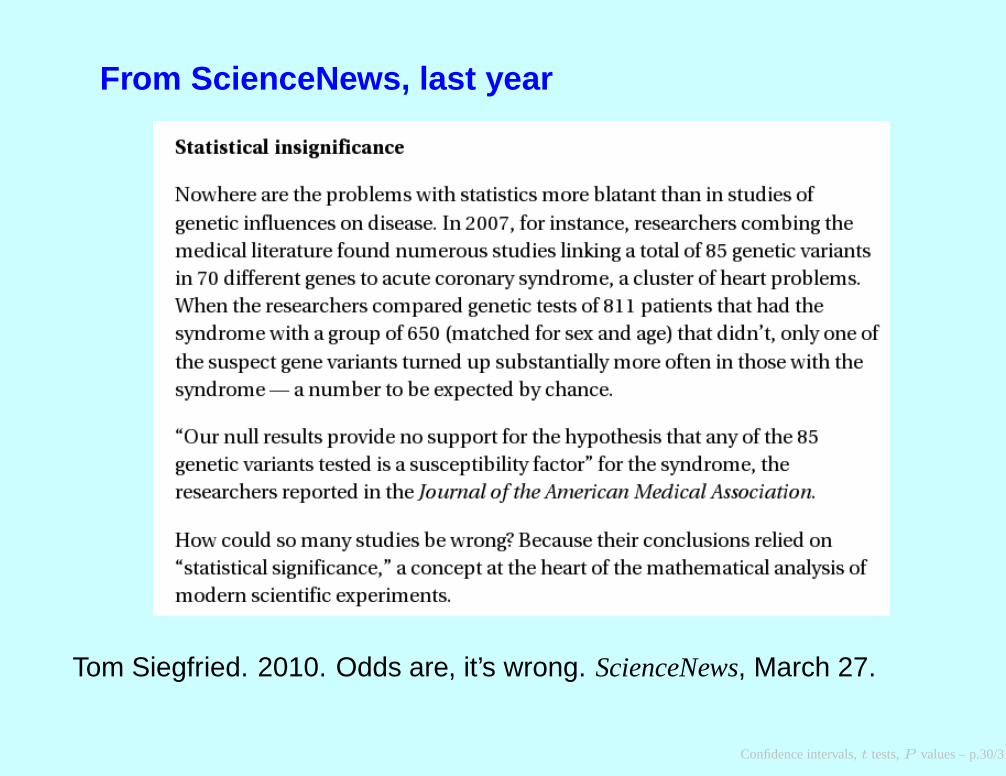
From ScienceNews, last year
Tom Siegfried. 2010. Odds are, it’s wrong. ScienceNews, March 27.
Confidence intervals,t tests,P values – p.30/31
MiscellaneousIf the two samples seem to have different variances, maybe you are on thewrong scale. Maybe their logarithms are normally distributed and haveequal variances (more nearly anyway). If we are dealing withmeasurements that can’t be negative, such as weights, that is a morenatural assumption, and sometimes it homogenizes the variances nicely.
Get familiar with the lognormal distribution, which just means the logs arenormally distributed. (It doesn’t matter whether natural logs or commonlogs as those are just multiples of each other).
Confidence intervals,t tests,P values – p.31/31