Confidence and the Transmission of Policy Shocks∗

Ruediger Bachmann

University of Michigan and NBER

Eric R. Sims

University of Notre Dame and NBER

August 11, 2010

Abstract

A widespread belief amongst economists, policy-makers, and members of the media

is that the “confidence”of households and firms is a critical component of the trans-

mission of fiscal and monetary policys shocks into economic activity. In this paper

we take this proposition to the data. We use common restrictions from the literature

to identify monetary and fiscal policy shocks in multivariate systems augmented with

measures of consumer and/or business confidence. We then construct counterfactual

impulse responses in which the endogenous response of confidence to policy is “shut

down”. Comparing the unconstrained and counterfactual responses of economic aggre-

gates allows us to determine the importance of confidence as a transmission mechanism

of policy. Typically, the counterfactual responses of GDP are dampened compared to

the unconstrained ones. Confidence, depending on the specification, can account for as

much as 100 percent of the quantitative magnitude of the responses, though often the

counterfactual responses of GDP are insignificantly different from the unconstrained

responses. Confidence appears to be more important in the transmission of tax and

monetary policy shocks than spending shocks, and business confidence is quantitatively

more important than consumer confidence.

∗Contact information: rudib@umich.edu and esims1@nd.edu. We are grateful to seminar participants atNotre Dame and Rochester for helpful comments and suggestions. Any remaining errors are our own.

“But the hope that monetary and fiscal policies would prevent continued weakness by boosting

consumer confidence was derailed by the recent report that consumer confidence in January

collapsed to the lowest level since 1992.” —Martin Feldstein, Wall Street Journal, February

20, 2008

“Confidence matters independently of fundamentals!”—Roger Farmer, May 29, 2010

1 Introduction

A widespread belief amongst economists, policy-makers, and members of the news media is

that the “confidence” of households and firms is a critical component of the transmission

of policy shocks into economic activity. A sampling of quotes from economists and policy-

makers with wide-ranging economic and political philosophies attest to this fact (see the

Appendix for more). A large literature studies the effects of fiscal and monetary policy

shocks on the real economy, while a smaller though not insubstantial literature examines the

effects of confidence in the economy. To our knowledge, however, no study bridges these two

literatures and explicitly examines the relationship between confidence and the transmission

of policy shocks. This paper fills that void.

We begin by reviewing some of the literature seeking to identify the effects of both fiscal

and monetary policy shocks in the economy. Most of these studies use the structural vector

autoregression (VAR) methodology, sometimes combined with an “event study”component,

to be described in more detail below. For fiscal policy, we examine the identification ap-

proaches of Blanchard and Perotti (2002), and Romer and Romer (2007). Blanchard and

Perotti combine institutional knowledge of the automatic stabilizer features of the tax and

spending system to identify both tax and spending shocks. Romer and Romer (2007) use

a narrative approach to come up with an exogenous tax changes series. For monetary pol-

icy, we use the Romer and Romer (1989) narrative approach, the Christiano, Eichenbaum,

and Evans (1999 and 2005) recursive VAR approaches, and the Romer and Romer (2004)

narrative-based approach.

Our paper is also related to the literature studying the effects of changes in consumer and

business confidence on economic activity. Carroll, Fuhrer, and Wilcox (1994), Matsusaka

and Sbordonne (1994), and Barsky and Sims (2010) try to measure how important changes in

confidence are in predicting the current and future paths of macroeconomic variables. This

literature hypothesizes that shocks to confidence may themselves be a source of economic

fluctuations, whereas in the current paper we study whether or not confidence is an important

source of the transmission and propagation of policy shocks.

1

To shed light on this question, we imbed measures of consumer and business confidence

into the VARs customarily used to identify monetary and fiscal policy shocks. We verify

that the inclusion of confidence in the system does little to alter either the qualitative or

quantitative dynamics of the response of economic activity to policy shocks. Further, con-

fidence typically responds in the way one would expect to policy shocks (i.e. contractionary

monetary policy shocks lead to reduced confidence). Business confidence tends to respond

both earlier and by more than does consumer confidence.

We then construct counterfactual impulse responses in which the level of confidence is held

constant in response to the policy shocks. In effect, this approach “turns off”the endogenous

response of confidence to policy, and in so doing also “turns off”the endogenous response

of activity to the endogenous response of confidence. Our methodology is an application

of an approach originally proposed in Sims and Zha (2006) to study the importance of

the systematic component of monetary policy. It has also been used to study the role of

monetary policy in the transmission of oil price shocks into the real economy (Bernanke,

Gertler, and Watson (1998) and Kilian and Lewis (2010)).

We find that confidence generally plays a modest role in the transmission and propagation

of policy shocks. In particular, “shutting down” the response of confidence to fiscal or

monetary policy shocks generally leads to an impulse response of output that is dampened

compared to the unconstrained impulse response, though the contribution of confidence is

in most cases statistically insignificant. Nevertheless, we find that confidence accounts from

anywhere between 100 percent and nothing of the response of real GDP to policy shocks.

Confidence appears to play a more important role in the transmission of monetary policy and

tax shocks than it does for government spending shocks. CEO confidence is also typically

a more important part of the transmission mechanism than is consumer confidence.

The remainder of the paper is organized as follows. Section 2 discusses potential mecha-

nisms why confidence might matter for the transmission of policy shocks. Section 3 reviews

the literature on identifying policy shocks. It also briefly reviews work examining the role of

confidence shocks in the aggregate economy. Section 4 provides detail on our counterfactual

impulse response methodology. Section 5 presents the results. The final section concludes,

and expounds on possible areas for future research.

2 Why Might Confidence Matter?

Within the conventions of dynamic general equilibrium rational expectations macroeco-

nomics, it is diffi cult to think of realistic theoretical structures which are capable of per-

mitting an important, independent role for “confidence”. The parameters of standard

2

neoclassical models capable of generating multiple equilibria (e.g. degree of returns to scale)

have been judged as empirically unrealistic (Basu and Fernald, 1997). Even under depar-

tures from full information rational expectations, general equilibrium forces and Bayesian

learning render pure confidence or sentiment fluctuations quantitatively irrelevant in many

contexts (Barsky and Sims, 2010). One important purpose of this paper is to attempt to use

minimal theory to inform the extent to which confidence matters, which in turn can guide

the development of more realistic macroeconomic models.

An old idea (Keynes, 1936) that has gained recent attention (Ackerlof and Shiller, 2008) is

that “animal spirits”are central to understanding economic fluctuations. While intriguing,

this idea lacks a coherent theoretical structure, and has met with limited empirical success

(Barsky and Sims, 2010). Loosely speaking, the idea is that aggregate sentiment determines

aggregate spending, which in turn determines aggregate output and employment. Fiscal

or monetary shocks from the government might signal a commitment to aggregate stability,

thereby raising sentiment, stimulating demand, and leading to economic expansion. This

idea is related to the “sunspot”framework popularized by Farmer (1998) and others, which

holds that there are, at any time, multiple aggregate equilibria. Stimulating sentiment could

cause the economy to jump from a “bad”equilibrium to a “good”one.

Another related possibility includes a role for informational frictions and strategic comple-

mentarities. In a world in which households fail to perfectly observe aggregate fundamentals

they may use observed variables (like aggregate output) to form perceptions of the true fun-

damentals (see Lorenzoni, 2009). Following a recession there might be induced sluggishness

—the true fundamentals might have improved but beliefs about the fundamentals are slow

to catch up, hence putting a brake on the recovery. By engaging in expansionary fiscal or

monetary policies, the government may be able to convince agents that fundamentals have

improved, thereby facilitating recovery.

Another possibility is that empirically measured confidence is a measure of a time-varying

discount factor —periods of high confidence are periods in which households do not discount

the future by much, and thus are relatively more willing to spend. If policies can lead to an

increase in confidence, they might therefore stimulate demand over and above what would

happen under normal transmission channels.

3 Related Literature

The purpose of this section is twofold. First, we briefly review some of the standard strategies

to identify both monetary and fiscal policy shocks. Second, we briefly review some of the

literature on confidence and its relation to our work.

3

As most of the identification schemes are (or can be) cast in a vector autoregression

framework, we briefly review some terminology before proceeding. A reduced form VAR

can be written as follows:

A(L)xt = ut

E(utu′t) = Σu 6= I

The vector of endogenous variables, xt, is dimension q×1. There are a variety of methods fordealing with trending variables in VARs, among them linear and quadratic detrending, HP

filtering, first differencing, estimating in levels, and estimating vector error correction models

in which cointegrating relationships are explicitly modeled. We proceed by estimating all

VARs in levels, which is the conservative approach advocated by Hamilton (1994). The

matrix A(L) = I−A1L − A2L2 − ... is a lag polynomial of order p. Under standard

assumptions, its elements can be consistently estimated via OLS. The vector ut is a vector

of innovations or time t forecast errors which may be correlated across equations.

It is assumed that there exists a linear mapping between structural shocks, of which there

are the same number as there are variables in the system, and reduced form innovations.

Structural shocks are defined as mutually uncorrelated innovations. The mapping between

structural and reduced form is:

ut = Bet

Normalizing the diagonal variance-covariance matrix of structural shocks to the identity

matrix, B is the solution toBB′ = Σu. This orthogonalizing matrix is not unique, andq(q−1)2

restrictions must be made in order to completely identify it. It is not necessary to impose

this many restrictions in order to identify only a subset of the shocks, however, which is an

approach frequently made in these literatures. A popular identifying assumption in these

literatures is that there is a recursive structure in which innovations to variables ordered late

in the system impact variables ordered early in the system only with a delay.1

3.1 Monetary Policy

We begin by reviewing popular methods for the identification of monetary policy shocks.

1This is not to say that recursiveness is the only assumption used to identify policy shocks. See Faust(1998) or Uhlig (2005) for alternative approaches to monetary policy identification and Mountford and Uhlig(2008) for fiscal policy.

4

3.1.1 Romer and Romer (1989)

Romer and Romer (1989) peruse the transcripts of FOMC meetings to come up with several

dates at which the US Federal Reserve exogenously pursued a contractionary policy aimed

at reducing inflation at the expense of real output. Focusing on the post-1960 data, these

dates are the fourth quarter of 1968, the second quarter of 1974, the third quarter of 1978,

and the fourth quarter of 1979.2

Let Dt be a dummy indicator taking a value of 1 in these quarters and zeros otherwise.

The vector of variables to be included in the VAR is xt = [yt Dt FFRt]′, where yt is

the log of real GDP and FFRt is the Federal Funds rate expressed at an annualized rate.3

The innovations are orthogonalized in the same order as the variables appear in xt, so that

the Romer dates only affect real GDP with a lag. They find that contractionary monetary

policy shocks are associated with a significant and persistent reduction in economic activity.

3.1.2 Christiano, Eichenbaum, and Evans (1999)

Christiano, Eichenbaum, and Evans (1999, hereafter CEE) estimate a benchmark VAR with

the log of real GDP, the log of the GDP deflator, a measure of commodity prices, the federal

funds rate, non-borrowed reserves, total reserves, and a measure of the money supply (either

M1 or M2). We estimate a variant of this dropping both non-borrowed and total reserves

and using M2 as our measure of the money supply.4 As with Romer and Romer (1989),

the identifying assumption is that monetary policy shocks (measured as innovations in the

federal funds rate), do not affect GDP or prices immediately, though they do affect the

money supply immediately. This amounts to a Choleski decomposition in which the funds

rate is ordered fourth. The remaining structural shocks are left unidentified.

3.1.3 Christiano, Eichenbaum, and Evans (2005)

CEE (2005) estimate a similar system to their 1999 paper. In particular, they include log

real GDP, log real consumption, log real investment, the GDP deflator, the real wage, labor

productivity, the federal funds rate, the growth rate of M2, and corporate profits in their

benchmark system. In addition, we include the same measure of commodity prices as above

2The original paper covers the entire post-war sample, including two additional dates in the 1950s. Westart the sample in the first quarter of 1960 because that is when the confidence data first become available.

3We aggregate the monthly FFR data to quarterly by taking the within quarter average. Alternativefrequency conversions (such as using the last monthly observation of the quarter) produce nearly identicalresults.

4Our measure of commodity prices is the BLS producer price index for intermediate inputs. We dropthe two reserve variables because, in a sample extended from their benchmark (which ends in 1996), thisresults in a high degree of collinearity with M2. The results are qualitatively invariant, however.

5

to help account for the price puzzle. The identifying restriction is the same as in the earlier

paper —most economic aggregates are restricted to not respond on impact to funds rate

innovations. In particular, only money growth and corporate profits are allowed to respond

to funds rate innovations within a quarter. This amounts to a Choleski decomposition in

which the funds rate is ordered eighth.

3.1.4 Romer and Romer (2004)

Romer and Romer (2004) extend the narrative analysis of their earlier paper. They combine

both quantitative and narrative records to form a measure of the exogenous changes in the

FOMC’s target funds rate. This differs from their earlier work in that the measure of

monetary policy here is a quantitative measure and not simply a qualitative dummy indicator.

The estimated system is otherwise similar to above —real GDP, the quantitative measure of

monetary policy shocks, and the fed funds rate. The innovations are orthogonalized such

that the policy shock has no immediate effect on output.5

3.2 Fiscal Policy

In this subsection we review the identification of fiscal shocks using VAR methods. Blan-

chard and Perotti (2002) identify both spending and tax shocks, while Romer and Romer

(2007) identify only tax shocks.6

3.2.1 Blanchard and Perotti (2002)

Blanchard and Perotti (2002) estimate a system featuring real government spending, real

tax collections, and real GDP. They assume that the reduced form innovations (call them

ug,t, uT,t, and uy,t, respectively) can be written as:

uT,t = a1uy,t + a2eg,t + et,t

ug,t = b1uy,t + b2eT,t + eg,t

uy,t = c1uT,t + c2ug,t + ey,t

5The paper uses monthly data with industrial production as the measure of activity. We aggregate theseries to a quarterly frequency by averaging within quarter.

6We also studied the “war date”-identification from Ramey (2009), which in turn is based on Ramey andShapiro (1998). The problem is that the Ramey/Shapiro dates are heavily influenced by the Korean wardate in the 1950s. We do not have confidence data going back this far. Running Ramey’s (2009) exactspecification on post-1960 data reveals that the war dates fail to predict significant changes in spending, sothat the interpretation of a multiplier is precarious at best here.

6

eg,t, eT,t, and ey,t, respectively, are the structural shocks. The coeffi cients a1 and b1 are

meant to capture the “automatic stabilizer”features of tax and spending. Estimates of a1and b1 are obtained outside of the VAR using institutional information. In the benchmark

identification, they impose that a1 = 2.08 and b1 = 0. Given these two restrictions, only one

more restriction is required to fully identify the system. The authors consider restricting

either a2 = 0 or b2 = 0. We consider the case with b2 = 0 as the benchmark, so that

spending does not respond to tax shocks within the quarter.7

3.2.2 Romer and Romer (2009)

Romer and Romer (2009) use the narrative approach to construct a measure of exogenous tax

changes, similarly to their (2007) monetary policy paper. In their benchmark identification,

they simply estimate a bivariate VAR with the tax measure and real GDP and construct the

impulse response of GDP.

3.3 Confidence

Another literature studies the effects of changes in measures of confidence for the evolution

of macroeconomic aggregates. Papers in this literature include Carroll, Fuhrer, and Wilcox

(1994), Matsusaka and Sbordonne (1994), and Barsky and Sims (2010). Carroll, Fuhrer,

and Wilcox (1994) show that changes in confidence have predictive content for future con-

sumption growth. They hypothesize that confidence proxies for current income, and test

whether a simple model with “rule of thumb”(Campbell and Mankiw, 1989) consumers can

account for the correlation. They find that changes in confidence have predictive content

for consumption growth above and beyond that which is contained in income.

Matsusaka and Sbordonne (1994) show that changes in confidence Granger cause changes

in economic aggregates, and argue in favor of models with multiple equilibria. Barsky and

Sims (2010) show that confidence innovations predict prolonged and (loosely speaking) per-

manent changes in both income and consumption. They argue that this result suggests

that confidence likely proxies for information agents have about future income that is other-

wise unavailable to econometricians, though they argue that there is likely not an important

direct causal channel between confidence and activity.

We draw on two sources for data on subjective measures of confidence —one for house-

holds and one for businesses. The first is the Survey of Consumers. Conducted by the

Survey Research Center at the University of Michigan, the survey polls a nationally repre-

sentative sample of households on a variety of questions concerning personal and aggregate

7The alternative assumption, a2 = 0, yields similar results.

7

economic conditions. Most answers are tabulated into qualitative categories —“good”, “neu-

tral”, and “bad”. Scores for each question are then tabulated as the percentage of good

responses minus the percentage of bad responses. These are then aggregated into an index,

which is known as the Index of Consumer Sentiment. Quarterly data from the survey are

publicly available beginning in the first quarter of 1960. The index is weighted to have value

of 100 as the first observation.

We obtain survey data on business confidence from the Conference Board’s CEO Confi-

dence Survey. The Conference Boards surveys CEOs in a variety of industries on current

and future economic conditions. As with the Michigan Survey, answers are tabulated into

qualitative categories —“very good”, “good”,“neutral”,“bad”, and “very bad”. These cate-

gories get a score of 100, 75, 50, 25, and 0, respectively. The aggregate confidence score is

simply the average across the respondents. Data from the survey are available at a quarterly

frequency beginning in 1976.

Figure 1 plots both series against time. The shaded gray areas are recessions as dated by

the National Bureau of Economic Research. Both series undergo repeated dramatic swings

and exhibit some of the properties that one might expect. For example, confidence is low

during recessions and high during booms. The CEO confidence data appear to lead the

business cycle more than do the confidence data. This unconditional feature of the data

turns out to also manifest itself in the conditional impulse responses.

Figure 2 plots impulse responses of real GDP from bivariate VARs with either measure of

confidence and real output, with both series in levels and the confidence innovation ordered

first. The dashed lines are 90 percent confidence intervals from Kilian’s bias-corrected boot-

strap after bootstrap. These figures replicate the essential insight of Barsky and Sims (2010):

confidence innovations, however measured, are associated with movements in output that are

much larger at long horizons than at short ones. The fact that confidence innovations have

a statistically significant effect on economy activity does not imply that confidence shocks

are an independent source of fluctuations; rather it is entirely consistent with confidence

innovations simply revealing information about other structural shocks. Barsky and Sims

(2010) conclude exactly this: changes in confidence are likely not an important independent

source of fluctuations. Their analysis is, however, silent on how confidence factors into the

transmission of other shocks into the economy.

4 Constructing Counterfactuals

We propose measuring the importance of confidence in the transmission of policy shocks by

constructing counterfactual impulse responses of macroeconomic variables to policy shocks

8

in which the endogenous response of confidence to the policy shock is “shut down”. This

necessitates first adding a measure of confidence to the VARs. For all systems, we include a

measure of confidence and order it last in the VARs. Ordering last means that confidence is

allowed to respond immediately to all of the other orthogonal shocks in the system (in par-

ticular policy shocks), while orthogonal innovations to confidence only affect macroeconomic

variables with a lag.

Using the VAR notation from above, the reduced form innovation in confidence (call it

uq+1,t) can be written as a linear combination of the other q orthogonalized shocks in the

system plus its own orthogonal innovation:

uq+1,t =

q∑j=1

bq+1,jej,t + eq+1,t

The bq+1,j are the coeffi cients in the q + 1th row of the orthogonalizing matrix B. If the

policy shock of interest is set to 1, for example, then the impact response of confidence to

policy would be given by bq+1,1.

The impulse response function is simply the structural moving average representation

of the time series. On impact, the impulse response is given by the impact matrix, B.

At subsequent horizons, h > 1, the response depends on both the impact matrix and the

reduced form moving average coeffi cients. Let IRFq+1,t(h) denote the impulse response of

confidence at horizon h to a unit jth orthogonal shock in the system. Write this as:

IRFq+1,j(h) = Cq+1,j(h)bq+1,j for j = 1, ..., q + 1

The elements Cq+1,j(h) are from the matrix polynomial of reduced form moving average

coeffi cients (i.e. C(L) = A(L)−1), with Cq+1,j(1) = 1 and bq+1,q+1 = 1.

The idea of constructing counterfactual impulse responses in a VAR context was first

proposed by Sims and Zha (2006) to determine how important the systematic component

of monetary policy (i.e. the endogenous response of the funds rate to other shocks) is for

the evolution of real variables. It was later also adopted in a similar context by Bernanke,

Gertler, and Watson (1998) to study the role of monetary policy in the transmission of oil

price shocks.

The counterfactual thought experiment can be applied as well to our problem and is both

conceptually and quantitatively straightforward. It involves constructing a time series of

counterfactual orthogonalized confidence shocks, eq+1,t, t = 1, ..., h, so as to set the impulse

response of confidence to a policy shock zero at all horizons. Using the above definition of

the impulse response function of confidence, and assuming that the policy shock is indexed

9

first and takes a value of unity, this amounts to the following recursive calculation of the

sequence of counterfactual orthogonal confidence innovations:

IRFq+1,j(h) = 0 ∀ h

⇔eq+1,1 = −bq+1,1eq+1,2 = − (Cq+1,1(2)bq+1,1 + Cq+1,q+1(2)eq+1,1)

eq+1,3 = − (Cq+1,1(3)bq+1,1 + Cq+1,q+1(3)eq+1,1 + Cq+1,q+1(2)eq+1,2)...

eq+1,h = −(Cq+1,q+1(h)bq+1,1 +

h−1∑j=1

Cq+1,q+1(h− 1− j)eq+1,j

)

Because orthogonal shocks to confidence affect the other variables of the system with a

lag, the counterfactual impulse responses will not only hold confidence fixed but will alter

the impulse responses of the other variables of the system. How much the responses of the

other variables (particularly real output) change when holding confidence fixed is precisely

the object of interest in our analysis.

We now briefly present some model-based evidence that our counterfactual methodology

is appropriate and likely to work well in practice. Formally, we operate under the null

hypothesis that confidence does not “matter”, though it may reflect available information

concerning underlying fundamentals. We study a simple DSGE model with government

spending shocks; similar results obtain in a framework where we study monetary policy

shocks.

Consider a simple version of a real business cycle (RBC) model in which government

spending evolves according to an exogenous, stochastic process and is financed via lump

sum taxation. The equilibrium of the economy can be characterized by the solution to a

planner’s problem:

maxct,kt+1,nt

E0

( ∞∑t=0

βt (ln ct + θ ln(1− nt)))

s.t.

10

ct + gt + kt+1 − (1− δ)kt = atkαt n

1−αt

ln at = ρa ln at−1 + ea,t

ln gt = (1− ρg) ln g∗ + ρg ln gt−1 + eg,t

We assume that the unconditional mean of log TFP is zero, or unity in the level. The

unconditional mean of government spending is g∗. We incorporate “confidence” into the

model in the following way: we assume that it follows a univariate AR(1) process with an

innovation equal to a linear combination of the two structural disturbances and its own

“noise”term:

conft = ρcconft−1 + φ1ea,t + φ2eg,t + ec,t

This specification is similar to the structural model in Barsky and Sims (2010) and is consis-

tent with the null hypothesis presented above: autonomous confidence “shocks”(ec,t) have

no effect on the real economy, but fundamental shocks can impact confidence if φ1 6= 0 orφ2 6= 0.We choose the following standard parameter values: α = 0.33, δ = 0.03, β = 0.98,

ρa = ρg = 0.9, and θ = 3. We then choose g∗ so that government spending is equal to 15

percent of output in steady state; with the parameterization of θ then about 25 percent of the

time endowment is spent working in steady state. We set φ1 = 1, φ2 = −0.5, and ρc = 0.9.We solve the model by linearizing the first order conditions about the non-stochastic steady

state. We set the standard deviations of the shocks to TFP, government spending, and

confidence at 0.007, 0.006, and 0.01, respectively.

We simulate data from the model, drawing shocks from normal distributions. Then for

each simulated data set we estimate a three variable VAR with government spending, output,

and confidence. We estimate the VAR in the levels of the variables with four lags. We

orthogonalize the innovations in that order using a Choleski decomposition. This ordering

is consistent with the implications of the structural model —government spending shocks

affect both output and confidence immediately; TFP shocks affect output and confidence

immediately but not government spending; and confidence shocks affect neither government

spending nor output on impact.

We simulate 500 data sets from the model with 200 observations each. Figure 3 shows

some results. The solid line depicts the theoretical impulse response to a government

spending shock in the model. The dashed line shows the average estimated response to

the identified government spending shock in the VAR across simulations. The shaded gray

11

areas are the 5th and 95th percentiles of the distribution of estimated responses. It is clear

that the VAR does a good job of identifying the model’s impulse responses. The responses

are roughly unbiased and capture well the model’s dynamic implications of a government

spending shock.

In the model as specified confidence declines in response to a government spending shock;

nevertheless, if confidence did not decline the impulse responses of output and government

spending to the government spending shock would be identical. Put differently, applying

our counterfactual methodology to the model-generated data should lead to no change in the

estimated impulse responses of output and government spending to the government spending

shock. Figure 4 shows results from this exercise. The solid line is the theoretical impulse

response; the dashed line is the average estimated response from the unrestricted identified

VAR; the dotted line shows the average responses from the counterfactual VARs; and the

shaded gray areas are the 5th and 95th percentiles of the distribution of unrestricted VAR

impulse responses. Here we see that there is essentially no difference in the unrestricted and

counterfactual impulse responses, which is consistent with the theory. By construction, the

confidence response is “shut down”.

This quantitative example is meant to be illustrative. It does, however, serve a couple

of purposes. First, it illustrates our methodology in a simple and transparent framework,

showing that it is likely to perform well. It also makes the following points clear: for

the counterfactual responses of aggregate variables to differ, (i) confidence must respond to

policy shocks and (ii) confidence innovations ordered last must have non-zero impacts on the

other variables over some horizon.

5 Results

We proceed similarly in this section as in Section 2. We augment the basic VAR systems

with a qualitative measure of confidence. We compute the impulse responses to the identified

shocks and then construct the counterfactual responses in which the confidence response is

“shut down”. We begin with monetary policy and then study fiscal policy.

5.1 Monetary Policy

5.1.1 Romer and Romer (1989)

Figure 5.1 shows impulse responses of GDP, the federal funds rate, and consumer confidence

from a three variable VAR as described above in Section 3.1.1. The sold lines are the unre-

stricted responses to a policy shock, with the shaded gray area representing the 90 percent

12

confidence bands, constructed via Kilian’s (1998) bias-corrected bootstrap after bootstrap.

The dashed lines show counterfactual responses holding confidence fixed. The time units

on the horizontal axis are quarters. The data used in the estimation span the 1960-2007

period.

In the unrestricted case, we see that the Romer “dates”are associated with a large and

persistent increase in the federal funds rate and a large decline in real GDP. The implied

“elasticity”of GDP to the policy shock (defined as the maximum percentage decline in GDP

over all horizons divided by the maximum percentage point increase in the funds rate) is

slightly greater than 1.5. Consumer confidence responds significantly and negatively to the

Romer “dates”, albeit with a lag, with peak negative response of confidence occurring a year

and a half after the shock.

The dashed line show the counterfactual responses. The counterfactual response of

the funds rate itself holding confidence fixed is virtually unchanged. The counterfactual

response of output is qualitatively similar to the unrestricted case but smaller. One is not

able to statistically reject the hypothesis that the responses are the same (i.e. the dashed

line lies within the shaded confidence region), but there is nevertheless some evidence that

confidence matters quantitatively. The “elasticity” (defined similar as above) of GDP to

the monetary policy shock is now -0.87 as opposed to -1.5, suggesting that as much as 40

percent of the response of output is due to consumer confidence.

Figure 5.2 repeats this exercise but uses CEO confidence in place of consumer confidence.

Qualitatively the results are very much the same —the funds rate response is almost identical

and the output response is similar but smaller. One important difference is that CEO

confidence reacts much more quickly to a policy shock than does consumer confidence. Here

the maximum decline in CEO confidence is on impact as opposed to at six quarters in the

case of consumer confidence.

5.1.2 CEE (1999)

In Figure 6.1 we show the responses to a monetary policy shock in CEE’s system augmented

with a measure of consumer confidence. The structure of the figures is the same as above.

In the unrestricted case, output declines significantly in response to the policy shock, albeit

with a substantial delay. Prices decline (but only with a very long delay) and the money

supply declines immediately. As one might expect, confidence declines, though once again

with a delay of several quarters.

The responses of the other variables in the system to the policy shock are very similar

in the counterfactual simulations. The hypothesis of equality between the restricted and

counterfactual responses for output can once again not be rejected at conventional levels of

13

significance. The unrestricted output elasticity with respect to the funds rate is here -0.76;

the elasticity under the counterfactual is -0.64. This suggests that confidence accounts for

only a little more than 10 percent of the response of output to a monetary policy shock.

Figure 6.2 conducts the same analysis using the CEO confidence survey. As was the

case with the Romer dates, CEO confidence falls most dramatically in the same quarter as

the shock, as opposed to several quarters later in the case of consumer confidence. While

still statistically insignificant, the counterfactual response of output to the policy shock is

roughly 50 percent of its value in the unrestricted case.

5.1.3 CEE (2005)

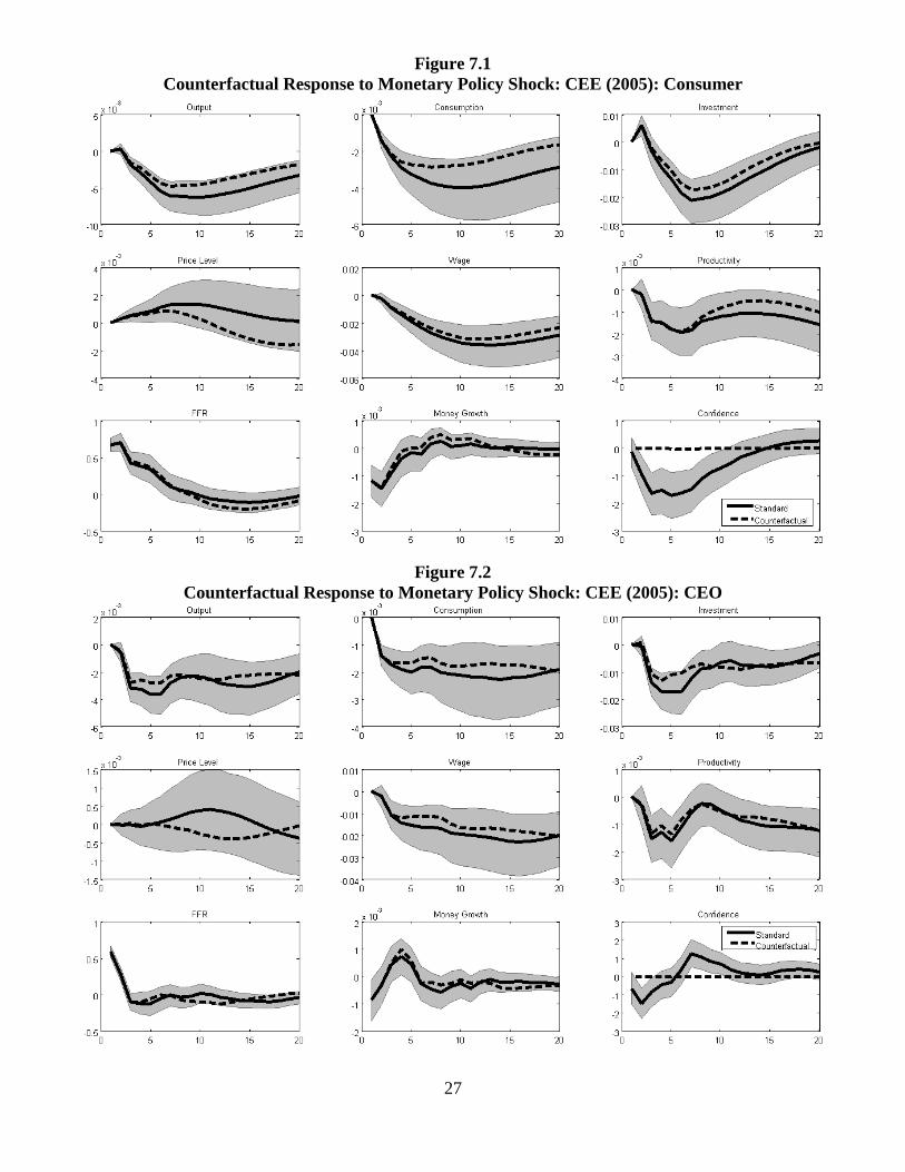
Figures 7.1 and 7.2 shows the analogous set of unrestricted and counterfactual responses for

the CEE (2005) system augmented with consumer and business confidence, respectively. In

the unrestricted case, the response of output looks very similar to the CEE (1999) responses.

In terms of the counterfactual responses, one observes that the responses of the variables

of the model to a monetary policy shock are roughly unchanged when forcing confidence to

not respond, though confidence itself does negatively and significantly respond to the shock

in the unrestricted system. The unrestricted elasticity of output with respect to the policy

shock is -0.9 here and the counterfactual elasticity is -0.68 when consumer confidence is held

fixed, or about 75% of its unrestricted value. In the case of CEO confidence, the results are

very much the same. CEO confidence declines sooner and more significantly does consumer

confidence. The counterfactual elasticity of output with respect the policy shock is also

roughly 75% of its unconstrained value.

5.1.4 Romer and Romer (2004)

In Figures 8.1 and 8.2 we show responses for the Romer and Romer (2004) identification. We

observe again that consumer confidence responds significantly and in the expected direction

to the contractionary monetary policy shock. Output responds less in the counterfactual

response than in the unrestricted response to the monetary policy shock, as we would expect,

though yet again the two responses are statistically indistinguishable. The unrestricted

elasticity of output with respect to money here is -0.57, while the restricted elasticity is -0.4.

The responses with CEO confidence tell much the same story.

5.1.5 Comments

For all four identifications of monetary policy shocks, we find that both consumer and busi-

ness confidence respond negatively and significantly to contractionary policy shocks. In

14

counterfactual simulations in which the response of confidence is held constant at its pre-

shock value, we find that real GDP responds less to the policy shock than in the unrestricted

case. The standard errors are, however, large, and it is not possible to statistically dis-

tinguish between the restricted and the unrestricted responses. The table below lists the

unrestricted and restricted elasticities of output to the federal funds rate, with this elasticity

defined as the maximum negative output response divided by the maximum positive funds

rate response, for both consumer and CEO confidence:

Table 1:Unrestricted and Counterfactual Monetary Policy Multipliers

Unrestricted Restricted Fraction Due to Confidence

Consumer Confidence:

Romer and Romer (1989) -1.5 -0.87 0.42

CEE (1999) -0.76 -0.64 0.16

CEE (2005) -0.90 -0.68 0.25

Romer and Romer (2004) -0.57 -0.40 0.30

CEO Confidence:

Romer and Romer (1989) -1.25 -0.80 0.35

CEE (1999) -0.49 -0.25 0.50

CEE (2005) -0.63 -0.48 0.23

Romer and Romer (2004) -0.58 -0.46 0.20

We can see that, in all four specifications, holding confidence fixed reduces the response

of output to policy shocks. The effects are higher for the two Romer and Romer narrative

identifications than for the recursive assumptions in the two CEE papers. We can con-

clude the confidence is likely a part of the transmission of monetary policy into real GDP,

though the effect is statistically diffi cult to distinguish from zero. There is little significant

quantitative difference between the results with consumer and CEO confidence.

5.2 Fiscal Policy

5.2.1 Blanchard and Perotti (2002)

Figure 9.1 shows the actual and counterfactual responses of the variables of interest to

both a government spending (upper panel) and a tax shock (lower panel) in the benchmark

Blanchard and Perotti (2002) identification in a system augmented to include consumer

confidence. In the unrestricted case, we see that an increase in spending leads to a mod-

est increase in output that is not very persistent. It also leads to a decline in consumer

15

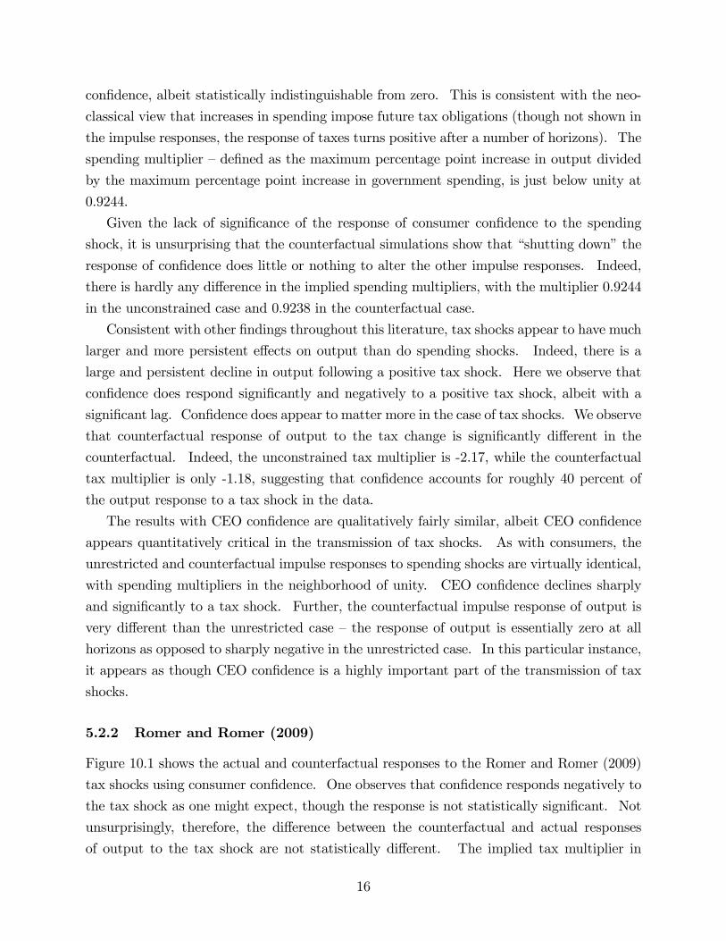
confidence, albeit statistically indistinguishable from zero. This is consistent with the neo-

classical view that increases in spending impose future tax obligations (though not shown in

the impulse responses, the response of taxes turns positive after a number of horizons). The

spending multiplier —defined as the maximum percentage point increase in output divided

by the maximum percentage point increase in government spending, is just below unity at

0.9244.

Given the lack of significance of the response of consumer confidence to the spending

shock, it is unsurprising that the counterfactual simulations show that “shutting down”the

response of confidence does little or nothing to alter the other impulse responses. Indeed,

there is hardly any difference in the implied spending multipliers, with the multiplier 0.9244

in the unconstrained case and 0.9238 in the counterfactual case.

Consistent with other findings throughout this literature, tax shocks appear to have much

larger and more persistent effects on output than do spending shocks. Indeed, there is a

large and persistent decline in output following a positive tax shock. Here we observe that

confidence does respond significantly and negatively to a positive tax shock, albeit with a

significant lag. Confidence does appear to matter more in the case of tax shocks. We observe

that counterfactual response of output to the tax change is significantly different in the

counterfactual. Indeed, the unconstrained tax multiplier is -2.17, while the counterfactual

tax multiplier is only -1.18, suggesting that confidence accounts for roughly 40 percent of

the output response to a tax shock in the data.

The results with CEO confidence are qualitatively fairly similar, albeit CEO confidence

appears quantitatively critical in the transmission of tax shocks. As with consumers, the

unrestricted and counterfactual impulse responses to spending shocks are virtually identical,

with spending multipliers in the neighborhood of unity. CEO confidence declines sharply

and significantly to a tax shock. Further, the counterfactual impulse response of output is

very different than the unrestricted case —the response of output is essentially zero at all

horizons as opposed to sharply negative in the unrestricted case. In this particular instance,

it appears as though CEO confidence is a highly important part of the transmission of tax

shocks.

5.2.2 Romer and Romer (2009)

Figure 10.1 shows the actual and counterfactual responses to the Romer and Romer (2009)

tax shocks using consumer confidence. One observes that confidence responds negatively to

the tax shock as one might expect, though the response is not statistically significant. Not

unsurprisingly, therefore, the difference between the counterfactual and actual responses

of output to the tax shock are not statistically different. The implied tax multiplier in

16

the unconstrained case is -1.88, which is not too different from the Blanchard and Perotti

(2002) results. The counterfactual tax multiplier is estimated to be -1.33, suggesting that

confidence accounts for roughly 30 percent of the response of GDP to a tax shock.

The results are similar in Figure 10.2, which shows unrestricted and counterfactual re-

sponses using the CEO confidence index. As in other figures, CEO confidence responds

sooner to the tax shock than does consumer confidence. The counterfactual response of

output is statistically indistinguishable from the unrestricted case, though confidence ac-

counts for as much as 50% of the quantitative magnitude of the response (particularly at the

long horizons).

5.2.3 Comments

We offer a brief concluding commentary on our counterfactual simulations for fiscal policy.

We find that confidence responds in the expected direction to fiscal shocks, typically much

more significantly to tax shocks than to spending shocks, which appears at first blush consis-

tent with neoclassical theories. We also find that confidence is a more important part of the

transmission mechanism of tax shocks than spending shocks. The table below summarizes

the implied actual and counterfactual multipliers.

Table 2:Unrestricted and Counterfactual Fiscal Policy Multipliers

Unrestricted Restricted Fraction Due to Confidence

Consumer Confidence:

BP (2002) Spending 0.92 0.92 0.00

BP (2002) Tax -2.17 -1.18 0.45

Romer and Romer (2007) Tax -1.88 -1.33 0.29

CEO Confidence:

BP (2002) Spending 1.10 1.09 0.00

BP (2002) Tax -1.51 0.00 1.00

Romer and Romer (2007) Tax -2.03 -1.05 0.50

These results suggest that confidence is potentially important in the transmission of tax

shocks, accounting for between one quarter and all of the output response. Confidence is

evidently completely unimportant in the transmission of spending shocks. We omit multi-

pliers based on Ramey (2009) due to the puzzling features of those responses. We observe

that CEO confidence is quantitatively about twice as important as consumer confidence in

transmission.

17

Many observers feel that fiscal policy is most potent when the economy exhibits extreme

slack (e.g. Christiano, Eichenbaum, and Rebelo, 2009). We experimented with a number of

non-linear specifications in which the impact effect of fiscal or tax shocks is different when

the economy is in a recession or when the unemployment rate is “high”(or more generally

when some cyclical indicator is “poor”). These specifications do not yield vastly different

impulse responses to policy shocks, and so we omit them for space consideration.

6 Conclusion

In this paper we have taken a serious look at an increasingly popular claim —that “confidence”

is an important part of the transmission mechanism between economic policy and economic

outcomes. We address this question by constructing counterfactual impulse responses to

identified policy shocks in which the response of confidence to policy is forced to equal

zero at all time horizons. Comparing the unrestricted and counterfactual responses of

economic variables allows us to quantify the importance of confidence in the transmission

and propagation of policy shocks.

Our results are somewhat mixed. In most cases, the counterfactual impulse responses

are statistically no different than the unrestricted cases. Quantitatively, however, the contri-

bution of confidence often appears large. In the case of tax shocks, confidence does appear

to be an important transmission mechanism, particular CEO confidence.

18

References

[1] Ackerlof, George and Robert Shiller. Animal Spirits. Princeton, NJ: Princeton Uni-

versity Press, 2008.

[2] Barsky, Robert B. and Eric Sims. “Information, Animal Spirits, and the Meaning of

Innovations in Consumer Confidence.” NBER WP #15049, 2010.

[3] Basu, Susanto and John Fernald. “Returns to Scale in US Production: Estimates and

Implications.” Journal of Political Economy 105, 249-283, 1997.

[4] Bernanke, Ben, Mark Gertler, and Mark Watson. “Systematic Monetary Policy and

the Effects of Oil Price Shocks.” Brookings Papers on Economic Activity, 1, 91-157,

1998.

[5] Blanchard, Olivier and Roberto Perotti. “An Empirical Characterization of the Dy-

namic Effects of Changes in Government Spending and Taxes on Output.” Quarterly

Journal of Economics. 107, 2002, 1329-12368.

[6] Campbell, John and N. Gregory Mankiw. “Consumption, Income, and Interest Rates:

Reinterpreting the Time Series Evidence.” NBER Macroeconomics Annual, 1989.

[7] Carroll, Christopher, Jeffrey Fuhrer and David Wilcox. “Does Consumer Sentiment

Forecast Household Spending? If so, Why?” American Economic Review, 1994, 1397-

1408.

[8] Christiano, Lawrence, Martin Eichenbaum, and Charles Evans. “Monetary Policy

Shocks: What Have We Learned and to What End?” Handbook of Macroeconomics,

1999.

[9] Christiano, Lawrence, Martin Eichenbaum, and Charles Evans. “Nominal Rigidities and

the Dynamic Effects of a Shock to Monetary Policy.” Journal of Political Economy,

2006, 514-558.

[10] Christiano, Lawrence, Martin Eichenbaum, and Sergio Rebelo. “When is the Govern-

ment Spending Multiplier Large?” NBER WP #15394, 2009.

[11] Farmer, Roger. The Macroeconomics of Self-Fulfilling Prophecies. Boston, MA: MIT

Press, 1998.

[12] Faust, Jon. “The Robustness of Identified VAR Conclusions About Money.” Carnegie-

Rochester Conference Series on Public Policy, 49, 1998, 207-244.

19

[13] Faust, Jon and Eric Leeper. “When Do Long Run Identifying Restrictions Given Reli-

able Results?” Journal of Business and Economics Statistics, 1997, 345-353.

[14] Keynes, John Maynard. The General Theory. 1936.

[15] Kilian, Lutz. “Small Sample Confidence Intervals for Impulse Response Functions.”

Review of Economics and Statistics, 1998, 218-230.

[16] Kilian, Lutz and Logan Lewis. “Does the Fed Respond to Oil Price Shocks?” University

of Michigan Working Paper, 2009.

[17] Lorenzoni, Guido. “A Theory of Demand Shocks.” American Economic Review 99:

2050-2084, 2009.

[18] Ramey, Valerie. “Identifying Government Spending Shocks: It’s All in the Timing.”

NBER WP #15464, 2009.

[19] Matsusaka, J.G. and Argia Sbordonne. “Consumer Confidence and Economic Fluctu-

ations.” Economic Inquiry. 1994.

[20] Mountford, Andrew and Harald Uhlig. “What are the Effects of Fiscal Policy Shock?”

Journal of Applied Econometrics, 24, 2009, 960-992.

[21] Romer, Christina and David Romer. “Does Monetary Policy Matter? A New Test in

the Spirit of Friedman and Schwartz.” NBER Macroeconomics Annual, 1989.

[22] Romer, Christina and David Romer. “A New Measure of Monetary Policy Shocks:

Derivation and Implications.” American Economic Review, 94, 1055-1084.

[23] Romer, Christina and David Romer. “The Macroeconomic Effects of Tax Changes:

Estimates Based on a New Measure of Fiscal Shocks.” American Economic Review,

forthcoming, 2009 (WP version 2007).

[24] Shapiro, Matthew and Valerie Ramey. “Costly Capital Reallocation and the Effects

of Government Spending.” Carnegie-Rochester Conference Series on Public Policy, 48,

1998, 145-194.

[25] Sims, Christopher and Tao Zha. “Does Monetary Policy Generate Recessions?”Macro-

economic Dynamics, 10, 2006, 231-272.

20

7 Appendix: Quotes“We must be certain that programs to solve the current financial and economic crisis are

large enough, and targeted broadly enough, to impact public confidence.”—Robert Shiller

“Yale’s Bob Shiller argues that confidence is the key to getting the economy back on track.

I think a lot of economists would agree with that.” —N. Gregory Mankiw

“Enacting such a conditional stimulus would have two desirable effects. First, it would im-

mediately boost the confidence of households and businesses since they would know that a

significant slowdown would be met immediately by a substantial fiscal stimulus.” —Martin

Feldstein

“But the hope that monetary and fiscal policies would prevent continued weakness by boosting

consumer confidence was derailed by the recent report that consumer confidence in January

collapsed to the lowest level since 1992.” —Martin Feldstein

“The economy is stagnant because of a lack of confidence in the future.” —Russell Roberts

“ . . . that at some point, people could lose confidence in the U.S. economy in a way that

could actually lead to a double-dip recession." —President Barack Obama

“The stimulus was too small, and it will fade out next year, while high unemployment is

undermining both consumer and business confidence.” —Paul Krugman

“It’s only an attempt to perhaps provide a bit of additional confidence, a bit of additional

assurance or a bit of additional certainty to the markets about the Federal Reserve’s long-term

objective.” —Ben Bernanke

“Economic activity in the United States turned up in the second half of 2009, supported by

an improvement in financial conditions, stimulus from monetary and fiscal policies, and a

recovery in foreign economies. These factors, along with increased business and household

confidence, appear likely to boost spending and sustain the economic expansion.” — Ben

Bernanke

“Confidence today will be enhanced if we put measures in place that assure that the coming ex-

pansion will be more sustainable and fair in the distribution of benefits than its predecessor.”

—Larry Summers

“President Obama’s top priority has been to stop the vicious cycle of economic and financial

collapse, stem the historic rate of job loss, restore confidence and put the economy on a path

21

to recover.”—Larry Summers

“Others say that we should have a fiscal stimulus to ’give people confidence,’even if we have

neither theory nor evidence that it will work.” —John Cochrane

“The subsequent global sell-off in equity markets suggested that governments would need to

take action with more immediate impact to restore confidence in the markets.” — James

Bullard

22

23

Figure 1: Consumer and Business Confidence Data

50

60

70

80

90

100

110

120

60 65 70 75 80 85 90 95 00 05 10

Index of Consumer Sentiment

20

30

40

50

60

70

80

1980 1985 1990 1995 2000 2005 2010

CEO Confidence

Note: Shades areas are recessions as defined by the NBER.

Figure 2 Impulse Responses to Confidence Innovations in Bivariate VAR

0 5 10 15 20 25 30 35 400.002

0.004

0.006

0.008

0.01

0.012

0.014

0.016

0.018

0.02

0.022GDP to Consumer Conf.

0 5 10 15 20 25 30 35 400

0.002

0.004

0.006

0.008

0.01

0.012

0.014GDP to CEO Conf.

Note: These are IRFs from two variable VARs with confidence and real GDP (with the confidence variable ordered first).

24

Figure 3 Impulse Response from Theoretical Model and Simulations

Note: the solid line shows the model impulse response to a government spending shock; the dashed line shows the average VAR estimated IRF across 500 simulations; and the shaded gray area shows the 5th and 95th percentiles of the distribution of estimated responses.

Figure 4 Counterfactual Impulse Responses from Model Simulation

Note: the dotted line shows the average estimated counterfactual impulse responses across the 500 simulations; see also the note to Figure 3.

25

Figure 5.1

Counterfactual Responses to Monetary Policy Shock: Romer and Romer (1989): Consumer

Figure 5.2

Counterfactual Responses to Monetary Policy Shock: Romer and Romer (1989): CEO

26

Figure 6.1 Counterfactual Responses to Monetary Policy Shock: CEE (1999): Consumer

Figure 6.2

Counterfactual Responses to Monetary Policy Shock: CEE (1999): CEO

27

Figure 7.1 Counterfactual Response to Monetary Policy Shock: CEE (2005): Consumer

Figure 7.2

Counterfactual Response to Monetary Policy Shock: CEE (2005): CEO

28

Figure 8.1 Counterfactual Response to Monetary Policy Shock: Romer and Romer (2004): Consumer

Figure 8.2

Counterfactual Response to Monetary Policy Shock: Romer and Romer (2004): CEO

29

Figure 9.1 Counterfactual Responses to Fiscal Policy: Blanchard and Perotti (2002): Consumer

Figure 9.2

Counterfactual Responses to Fiscal Policy: Blanchard and Perotti (2002): CEO

30

Figure 10.1 Counterfactual Response to Fiscal Policy: Romer and Romer (2009): Consumer

Figure 10.2

Counterfactual Response to Fiscal Policy: Romer and Romer (2009): CEO