PRODUCT 0-6332-P1 and P2TxDOT PROJECT NUMBER 0-6332

ConcreteWorks V3 Training/User Manual (P1)

ConcreteWorks Software (P2)

Research Supervisor:Kevin Folliard

July 2013; Published April 2017

http://library.ctr.utexas.edu/ctr-publications/0-6332-P1P2.pdf

0-6332-P1

CONCRETEWORKS V3 TRAINING/USER MANUAL Dr. Kyle Riding Dr. Anton Schindler Philip Pesek Dr. Thanos Drimalas Dr. Kevin Folliard Project 0-6332: Development of Predictive Model for Bridge Deck Cracking and

Strength Development JULY 2013; PUBLISHED APRIL 2017

Performing Organization: Center for Transportation Research The University of Texas at Austin 1616 Guadalupe Street, Suite 4.202 Austin, Texas 78701

Sponsoring Organization: Texas Department of Transportation Research and Technology Implementation Office P.O. Box 5080 Austin, Texas 78763-5080

Performed in cooperation with the Texas Department of Transportation and the Federal Highway Administration.

Acknowledgements

This program was made possible through funding provided by the Texas Department of Transportation. The advice of the following individuals is appreciated: Ralph Browne, Tyler Ley, Moon Won, Brian Merrill, Charles Gaskin, David Head, Doug Beer, J.C. Liu, John Vogel, Kevin Pruski, and Tom Yarbrough.

iii

Table of Contents

1. Introduction ........................................................................................................................... 1

2. Concrete Mixture Proportioning Guide ............................................................................. 2

2.1. Basic Mixture Proportioning ............................................................................................ 2 2.2. Water Adjustments ........................................................................................................... 3 2.3. Aggregate Gradations ....................................................................................................... 4

3. Temperature Prediction ....................................................................................................... 5

3.1. Heat Transfer Modeling ................................................................................................... 5 3.1.1. Fundamentals and Numerical Scheme ...................................................................... 5 3.1.2. Time Discretization ................................................................................................... 9 3.1.3. Symmetry ................................................................................................................ 10 3.1.4. Concrete Thermal Properties .................................................................................. 10 3.1.5. Concrete Heat of Hydration .................................................................................... 11 3.1.6. Boundary Conditions .............................................................................................. 13

3.2. Concrete Member Models .............................................................................................. 14 3.2.1. Rectangular Column ............................................................................................... 14 3.2.2. Rectangular Footing ................................................................................................ 18 3.2.3. Rectangular Footing with Soil on the Sides ............................................................ 21 3.2.4. Bent Caps ................................................................................................................ 23 3.2.5. T-Shaped Bent Cap ................................................................................................. 27 3.2.6. Circular Columns .................................................................................................... 30 3.2.7. Bridge Decks ........................................................................................................... 31 3.2.8. Precast Rectangular and U-Shaped Beams ............................................................. 33 3.2.9. Precast Type IV Beams ........................................................................................... 35 3.2.10. Pavements ............................................................................................................ 37

4. Thermal Stress Analysis ..................................................................................................... 40

4.1. Overview ........................................................................................................................ 40 4.2. Plastic Shrinkage ............................................................................................................ 42 4.3. Free Shrinkage and Mechanical Properties .................................................................... 42

4.3.1. Concrete Maturity and Strength Development ....................................................... 42 4.3.2. Poisson Ratio .......................................................................................................... 45 4.3.3. Coefficient of Thermal Expansion .......................................................................... 47 4.3.4. Autogenous Shrinkage Model................................................................................. 49

4.4. Elastic Stress and Degree of Restraint ........................................................................... 50 4.5. Early-Age Concrete Creep Model .................................................................................. 51

iv

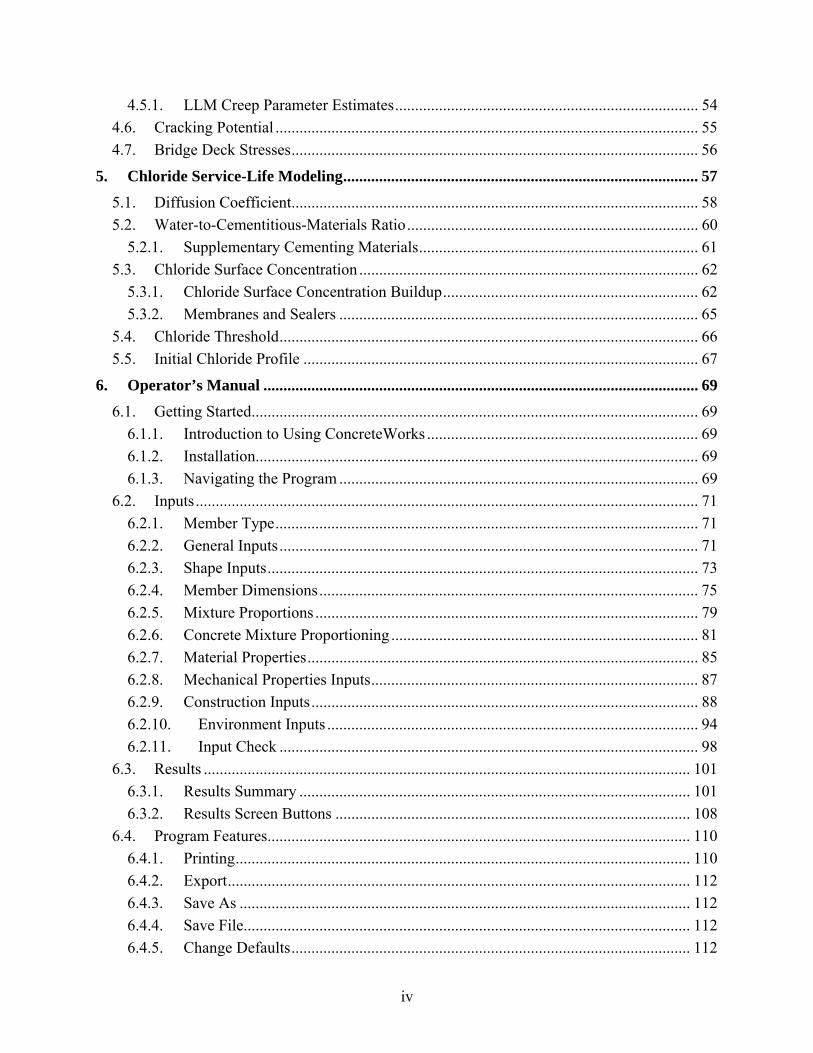
4.5.1. LLM Creep Parameter Estimates ............................................................................ 54 4.6. Cracking Potential .......................................................................................................... 55 4.7. Bridge Deck Stresses ...................................................................................................... 56

5. Chloride Service-Life Modeling ......................................................................................... 57

5.1. Diffusion Coefficient ...................................................................................................... 58 5.2. Water-to-Cementitious-Materials Ratio ......................................................................... 60

5.2.1. Supplementary Cementing Materials ...................................................................... 61 5.3. Chloride Surface Concentration ..................................................................................... 62

5.3.1. Chloride Surface Concentration Buildup ................................................................ 62 5.3.2. Membranes and Sealers .......................................................................................... 65

5.4. Chloride Threshold ......................................................................................................... 66 5.5. Initial Chloride Profile ................................................................................................... 67

6. Operator’s Manual ............................................................................................................. 69

6.1. Getting Started ................................................................................................................ 69 6.1.1. Introduction to Using ConcreteWorks .................................................................... 69 6.1.2. Installation............................................................................................................... 69 6.1.3. Navigating the Program .......................................................................................... 69

6.2. Inputs .............................................................................................................................. 71 6.2.1. Member Type .......................................................................................................... 71 6.2.2. General Inputs ......................................................................................................... 71 6.2.3. Shape Inputs ............................................................................................................ 73 6.2.4. Member Dimensions ............................................................................................... 75 6.2.5. Mixture Proportions ................................................................................................ 79 6.2.6. Concrete Mixture Proportioning ............................................................................. 81 6.2.7. Material Properties .................................................................................................. 85 6.2.8. Mechanical Properties Inputs .................................................................................. 87 6.2.9. Construction Inputs ................................................................................................. 88 6.2.10. Environment Inputs ............................................................................................. 94 6.2.11. Input Check ......................................................................................................... 98

6.3. Results .......................................................................................................................... 101 6.3.1. Results Summary .................................................................................................. 101 6.3.2. Results Screen Buttons ......................................................................................... 108

6.4. Program Features.......................................................................................................... 110 6.4.1. Printing .................................................................................................................. 110 6.4.2. Export .................................................................................................................... 112 6.4.3. Save As ................................................................................................................. 112 6.4.4. Save File................................................................................................................ 112 6.4.5. Change Defaults .................................................................................................... 112

v

6.4.6. Tools Menu ........................................................................................................... 113 6.4.7. Help Menu ............................................................................................................ 114

6.5. Input Sensitivities ......................................................................................................... 114 6.5.1. Environment Inputs Sensitivity ............................................................................ 114 6.5.2. Run Speed ............................................................................................................. 114

6.6. Troubleshooting ........................................................................................................... 115 6.6.1. Installation Problems ............................................................................................ 115 6.6.2. Screen Settings ...................................................................................................... 115

References .................................................................................................................................. 116

vii

List of Tables

Table 1 - Software features available for each concrete member type ........................................... 1 Table 2 - Concrete water requirement and coarse aggregate volume fit parameters based

on the maximum size aggregate ................................................................................................ 3 Table 3 - Range of water adjustment factors used in ConcreteWorks (Hover, 2003) .................... 4 Table 4 - Corners of box of acceptable mixtures for Shilstone Coarseness Factor-

Workability Factor aggregate gradation method (TxDOT Special Provision 421) .................. 5 Table 5 - Chemical admixture dosages assumed in ConcreteWorks ............................................ 13 Table 6 - Footing subbase material thermal properties ................................................................. 20 Table 7 - Pavement subbase material properties ........................................................................... 39 Table 8 - CTE for concretes made with different aggregates (Bamforth and Price, 1995) .......... 47 Table 9 - Concrete constituent materials assumed specific gravity values ................................... 49 Table 10 - Concrete constituent materials assumed CTE ............................................................. 49 Table 11 - Modified linear logarithmic model parameters assumed to remain constant in

ConcreteWorks ....................................................................................................................... 55 Table 12 - Chloride surface concentration constants used in ConcreteWorks for marine

exposure .................................................................................................................................. 64 Table 13 - Build-up rate constants with their corresponding maximum surface

concentration values used in ConcreteWorks ......................................................................... 65 Table 14 - Chloride threshold values assumed for black steel based on corrosion inhibitor

dose ......................................................................................................................................... 67 Table 15 - Values deemed questionable by ConcreteWorks ...................................................... 100

ix

List of Figures

Figure 1 - Control volume example - three neighboring nodes ...................................................... 7 Figure 2 - Example of control volume with a convection boundary condition .............................. 9 Figure 3 - Horizontal cross section of rectangular column assumed in ConcreteWorks .............. 15 Figure 4 - Simplified rectangular column model used in ConcreteWorks ................................... 15 Figure 5 - Example rectangular column node and control volumes ............................................. 16 Figure 6 - Rectangular column during form removal and the beginning of construction

stage two ................................................................................................................................. 17 Figure 7 - Diagram of the vertical cross section assumed in modeling a two-dimensional

footing ..................................................................................................................................... 18 Figure 8 - Summary of rectangular footing boundary conditions ................................................. 19 Figure 9 - Rectangular footing model ........................................................................................... 20 Figure 10 - Node layout for rectangular footing ........................................................................... 21 Figure 11 - Summary of rectangular footing with soil on the sides .............................................. 22 Figure 12 - Rectangular footing with “soil on sides” model ........................................................ 22 Figure 13 - Node and control volume layout for rectangular footing with soil on the sides ........ 23 Figure 14 - Diagram of the vertical cross section modeled in a rectangular bent cap .................. 24 Figure 15 - Rectangular bent cap radiation summary ................................................................... 24 Figure 16 - Rectangular bent cap convection summary ................................................................ 25 Figure 17 - Summary of rectangular bent cap .............................................................................. 26 Figure 18 - Node and control volume layout of rectangular bent cap .......................................... 26 Figure 19 - Summary of dolphin with pre-cast concrete bottom .................................................. 27 Figure 20 - Summary of radiation boundary conditions for T-shaped bent caps ......................... 28 Figure 21 - Summary of convection boundary conditions on T-shaped bent cap ........................ 28 Figure 22 - Construction summary form T-shaped bent cap ........................................................ 29 Figure 23 - Node and control volume layout for T-shaped bent caps .......................................... 29 Figure 24 - Circular column model ............................................................................................... 30 Figure 25 - Node and control volume layout for circular columns ............................................... 31 Figure 26 - Circular column boundary conditions ........................................................................ 31 Figure 27 - Bridge deck layout ..................................................................................................... 32 Figure 28 - Bridge deck node and control volume layout ............................................................ 32 Figure 29 - Bridge deck temperature boundary conditions .......................................................... 33 Figure 30 - Modeled region of rectangular and U-shaped beams ................................................. 34 Figure 31 - ConcreteWorks simplified model for rectangular and U-shaped beams ................... 34 Figure 32 - Rectangular and U-shaped beam node and control volume layout ............................ 35 Figure 33 - Precast type IV beam model assumed in ConcreteWorks ......................................... 36 Figure 34 - Precast type IV beam node and control volume boundary layout ............................. 36

x

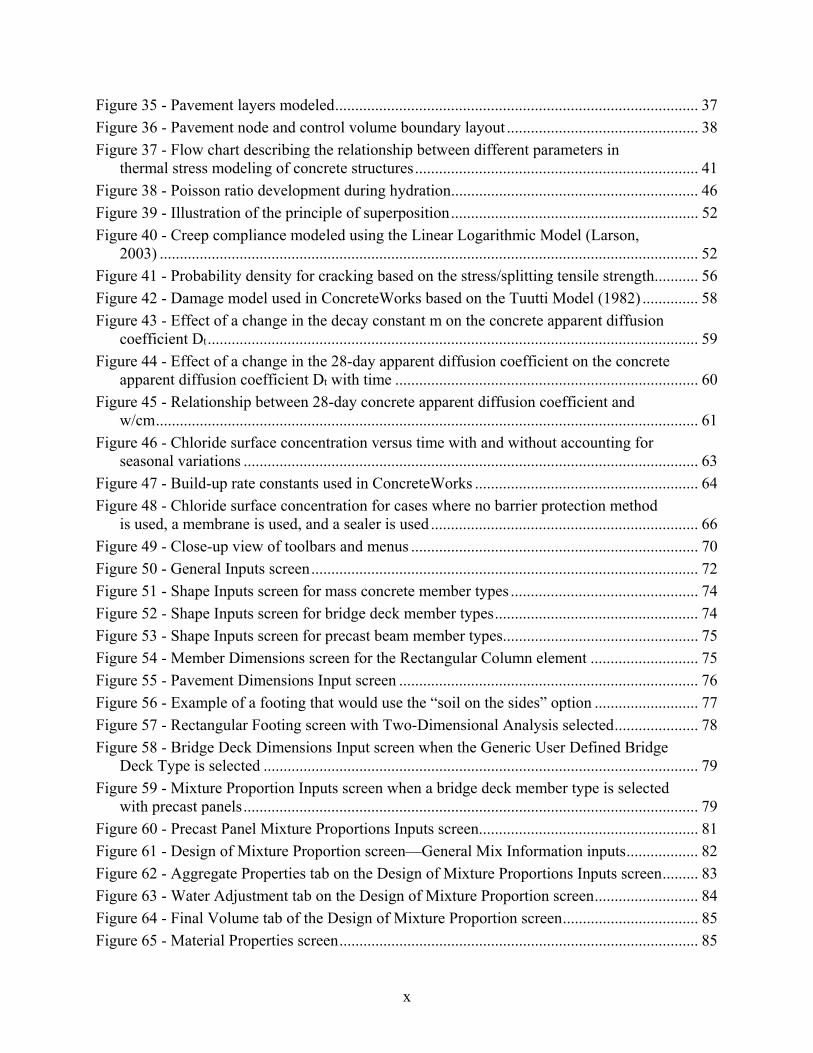
Figure 35 - Pavement layers modeled ........................................................................................... 37 Figure 36 - Pavement node and control volume boundary layout ................................................ 38 Figure 37 - Flow chart describing the relationship between different parameters in

thermal stress modeling of concrete structures ....................................................................... 41 Figure 38 - Poisson ratio development during hydration .............................................................. 46 Figure 39 - Illustration of the principle of superposition .............................................................. 52 Figure 40 - Creep compliance modeled using the Linear Logarithmic Model (Larson,

2003) ....................................................................................................................................... 52 Figure 41 - Probability density for cracking based on the stress/splitting tensile strength ........... 56 Figure 42 - Damage model used in ConcreteWorks based on the Tuutti Model (1982) .............. 58 Figure 43 - Effect of a change in the decay constant m on the concrete apparent diffusion

coefficient Dt ........................................................................................................................... 59 Figure 44 - Effect of a change in the 28-day apparent diffusion coefficient on the concrete

apparent diffusion coefficient Dt with time ............................................................................ 60 Figure 45 - Relationship between 28-day concrete apparent diffusion coefficient and

w/cm ........................................................................................................................................ 61 Figure 46 - Chloride surface concentration versus time with and without accounting for

seasonal variations .................................................................................................................. 63 Figure 47 - Build-up rate constants used in ConcreteWorks ........................................................ 64 Figure 48 - Chloride surface concentration for cases where no barrier protection method

is used, a membrane is used, and a sealer is used ................................................................... 66 Figure 49 - Close-up view of toolbars and menus ........................................................................ 70 Figure 50 - General Inputs screen ................................................................................................. 72 Figure 51 - Shape Inputs screen for mass concrete member types ............................................... 74 Figure 52 - Shape Inputs screen for bridge deck member types ................................................... 74 Figure 53 - Shape Inputs screen for precast beam member types ................................................. 75 Figure 54 - Member Dimensions screen for the Rectangular Column element ........................... 75 Figure 55 - Pavement Dimensions Input screen ........................................................................... 76 Figure 56 - Example of a footing that would use the “soil on the sides” option .......................... 77 Figure 57 - Rectangular Footing screen with Two-Dimensional Analysis selected ..................... 78 Figure 58 - Bridge Deck Dimensions Input screen when the Generic User Defined Bridge

Deck Type is selected ............................................................................................................. 79 Figure 59 - Mixture Proportion Inputs screen when a bridge deck member type is selected

with precast panels .................................................................................................................. 79 Figure 60 - Precast Panel Mixture Proportions Inputs screen ....................................................... 81 Figure 61 - Design of Mixture Proportion screen—General Mix Information inputs .................. 82 Figure 62 - Aggregate Properties tab on the Design of Mixture Proportions Inputs screen ......... 83 Figure 63 - Water Adjustment tab on the Design of Mixture Proportion screen .......................... 84 Figure 64 - Final Volume tab of the Design of Mixture Proportion screen .................................. 85 Figure 65 - Material Properties screen .......................................................................................... 85

xi

Figure 66 - Material Inputs screen with manual adjustment checkboxes checked ....................... 86 Figure 67 - Mechanical Properties inputs ..................................................................................... 87 Figure 68 - Construction Inputs screen for a rectangular column ................................................ 89 Figure 69 - Construction Inputs screen shown when the rectangular footing member

shape is chosen ........................................................................................................................ 91 Figure 70 - Construction Inputs screen for a rectangular bent cap with pre-cast concrete

selected as the bottom form .................................................................................................... 92 Figure 71 - Bridge Deck inputs when wood forms are selected ................................................... 93 Figure 72 - Pavement Construction inputs .................................................................................... 94 Figure 73 - Temperature tab on the Environment Inputs screen .................................................. 95 Figure 74 - Percent Cloud Cover tab on the Environment Inputs screen ..................................... 96 Figure 75 - Yearly Temperature inputs ......................................................................................... 97 Figure 76 - Summary Graphs tab on the Environment Inputs screen (the temperature

graph is currently displayed) ................................................................................................... 98 Figure 77 - Input Check screen ..................................................................................................... 99 Figure 78 - Mix Checks tab shown on the Rectangular Column Temperature Model

screen .................................................................................................................................... 102 Figure 79 - Max-Min Graph tab as shown on the Rectangular Column Temperature

Model screen ......................................................................................................................... 103 Figure 80 - Animation tab as shown on the Rectangular Column Temperature Model

screen .................................................................................................................................... 104 Figure 81 - Maturity tab as shown on the Rectangular Column Temperature Model screen ..... 105 Figure 82 - Compressive Strength tab with compressive strength calculated as shown on

the Rectangular Column Temperature Model screen ........................................................... 106 Figure 83 - Graph of chloride concentration at steel .................................................................. 107 Figure 84 - Cracking risk classification chart ............................................................................. 108 Figure 85 - Comparison chart screen .......................................................................................... 109 Figure 86 - Rectangular Footing Results screen with the Cross-Section to be Displayed

frame showing ....................................................................................................................... 110 Figure 87 - Print Preview screen ................................................................................................. 111 Figure 88 - Page Setup dialog ..................................................................................................... 112 Figure 89 - Material Inputs tab on the Change Defaults screen ................................................. 113

1

1. Introduction

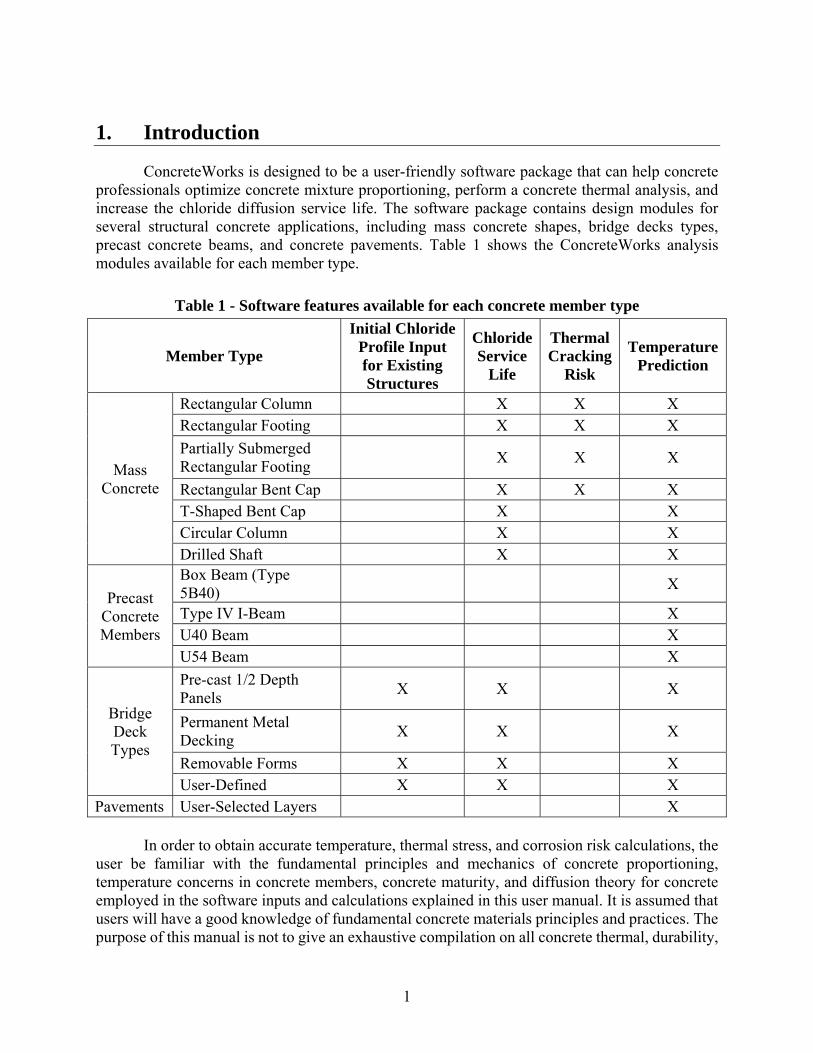
ConcreteWorks is designed to be a user-friendly software package that can help concrete professionals optimize concrete mixture proportioning, perform a concrete thermal analysis, and increase the chloride diffusion service life. The software package contains design modules for several structural concrete applications, including mass concrete shapes, bridge decks types, precast concrete beams, and concrete pavements. Table 1 shows the ConcreteWorks analysis modules available for each member type.

Table 1 - Software features available for each concrete member type

Member Type

Initial Chloride Profile Input for Existing Structures

Chloride Service

Life

Thermal Cracking

Risk

Temperature Prediction

Mass Concrete

Rectangular Column X X X Rectangular Footing X X X

Partially Submerged Rectangular Footing

X X X

Rectangular Bent Cap X X X T-Shaped Bent Cap X X Circular Column X X Drilled Shaft X X

Precast Concrete Members

Box Beam (Type 5B40)

X

Type IV I-Beam X U40 Beam X U54 Beam X

Bridge Deck Types

Pre-cast 1/2 Depth Panels

X X X

Permanent Metal Decking

X X X

Removable Forms X X X User-Defined X X X

Pavements User-Selected Layers X

In order to obtain accurate temperature, thermal stress, and corrosion risk calculations, the user be familiar with the fundamental principles and mechanics of concrete proportioning, temperature concerns in concrete members, concrete maturity, and diffusion theory for concrete employed in the software inputs and calculations explained in this user manual. It is assumed that users will have a good knowledge of fundamental concrete materials principles and practices. The purpose of this manual is not to give an exhaustive compilation on all concrete thermal, durability,

2

and corrosion research in the literature. Instead, this manual is designed assist the user with the specific knowledge of concrete behavior needed to successfully use ConcreteWorks, built upon an already existing knowledge of fundamental concrete behavior. It is recommended that users carefully read this user manual as well as cited references as needed before using the software.

This manual is divided into an informational section followed by an operator’s manual. Chapter 2 presents the information on the ConcreteWorks mixture proportioning guide. Chapter 3 describes how the heat transfer calculations in the program are performed. Chapter 4 explains how the program’s thermal stress analysis and consequent cracking risk assessment is done. Chapter 5 discusses the chloride service life model built into ConcreteWorks. Finally, a ConcreteWorks operator’s manual is provided in Chapter 6.

2. Concrete Mixture Proportioning Guide

2.1. Basic Mixture Proportioning

The backbone for the mixture proportioning guide found in ConcreteWorks is the procedure outlined in the ACI 211 document “Standard Practice for Selecting Proportions for Normal, Heavyweight, and Mass Concrete” (ACI 211, 1991). For a detailed explanation of this mixture proportioning method, users are encouraged to read the ACI 211.1-91 document.

The basic steps of the concrete mixture proportioning procedure can be summarized as the following:

1. Determine the amount of water needed to achieve a given slump for the selected maximum aggregate size. Adjust the required water amount based on material conditions, chemical admixtures, air entrainment, etc. (covered in Section 2.2 of this document).

2. Determine the water-to-cementitious-materials ratio (w/cm) needed for a given air content to achieve selected target strength. The use of supplementary materials is assumed to not affect the w/cm needed to achieve the target strength (which may or may not be true depending on the reactivity of the material and the replacement rate). Supplementary cementing materials replacement percentages are only used in calculating the volume of cementitious materials.

3. Adjust the w/cm to account for maximum w/cm allowed for given exposure conditions (chloride and sulfate exposure levels).

4. Calculate the coarse aggregate fraction based on the maximum size aggregate, the sand fineness modulus, and the coarse aggregate dry-rodded unit weight.

5. Calculate the amount of sand needed to fill the remaining concrete volume (that volume not already accounted for by the cementitious materials, water, coarse aggregate, or air). The sand weight is then calculated for this volume using the sand specific gravity. The required water amount is calculated using Equation 1 and the coefficients found in Table

1 based on the ACI 211.1-91 Table 6.3.3. The required water amount is then reduced by the percentages specified using the water adjustment factors discussed in Section 2.2 and calculated using Equation 1:

)1())ln(( WAbslaW ww −⋅+⋅= Equation 1

3

where W is the required water (lb/yd³), aw and bw are constants determined from Table 2 (lb/yd³), sl is the desired concrete slump (in), and WA is the water reduction factor. The amount of water needed to obtain the required slump increases as the maximum aggregate size decreases and consequently the total aggregate surface area increases.

Table 2 - Concrete water requirement and coarse aggregate volume fit parameters based on the maximum size aggregate

Maximum Aggregate Size (in.)

aw (lb/yd³)

bw (lb/yd³)

aca

2 27.411 249.41 0.78 1.5 27.411 264.41 0.75 1 27.411 289.41 0.71

0.75 30.618 302.31 0.66 0.5 34.176 321.45 0.59

0.375 40.941 333.49 0.5

The connection between compressive strength and w/cm was first published in 1918 by Duff Abrams. W/cm is one of the major factors in determining the concrete porosity and consequently compressive strength (Mindess, Young, and Darwin, 2003). Air entrainment will increase the amount of voids in concrete, and consequently reduce the strength. The required w/cm ratio is calculated using Equation 2 through Equation 4:

))ln((/ '

acta bfacmw +⋅= Equation 2

3762.0*00065.0 −= airaa Equation 3

7275.3*0263.0 −−= airba Equation 4where air is the target percent air in the concrete, and fct’ is the concrete target strength. Equations 3 and 4 were calculated using a regression analysis from the data found in ACI 211.1-91 table 6.3.4, assuming the quoted values of 2% entrapped air for the non-air entrained concrete and 6% for the air entrained concrete.

The coarse aggregate weight is calculated using Equation 5:

DRUWFM

aCAW ca ⋅−+= )10

)4.2(( Equation 5

where CAW is the coarse aggregate weight (lb/yd3), aca is a fit parameter found in Table 2, FM is the fineness modulus, and DRUW is the coarse aggregate dry rodded unit weight (lb/yd3). The coefficient aca was derived by fitting the data found in ACI 211.1-91 Table 6.3.6.

2.2. Water Adjustments

The required water adjustments procedures and magnitudes are based on the National Highway Institute (NHI) Course 15123 Participant Workbook (Hover, 2003). The amount of water adjustment needed for each material used is highly material dependent. Concrete mixture proportioning knowledge and experience with the local materials used is critical to accurately

4

estimate the influence of each material on the concrete mixture. A trial batch is normally required to confirm the validity of the concrete mixture designed, and to make any necessary adjustments to the concrete workability.

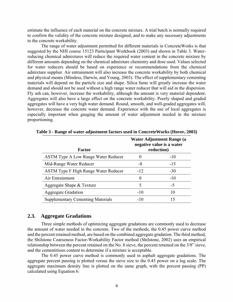
The range of water adjustment permitted for different materials in ConcreteWorks is that suggested by the NHI course 15123 Participant Workbook (2003) and shown in Table 3. Water-reducing chemical admixtures will reduce the required water content in the concrete mixture by different amounts depending on the chemical admixture chemistry and dose used. Values selected for water reducers should be based on experience or recommendations from the chemical admixture supplier. Air entrainment will also increase the concrete workability by both chemical and physical means (Mindess, Darwin, and Young, 2003). The effect of supplementary cementing materials will depend on the particle size and shape. Silica fume will greatly increase the water demand and should not be used without a high range water reducer that will aid in the dispersion. Fly ash can, however, increase the workability, although the amount is very material dependent. Aggregates will also have a large effect on the concrete workability. Poorly shaped and graded aggregates will have a very high water demand. Round, smooth, and well-graded aggregates will, however, decrease the concrete water demand. Experience with the use of local aggregates is especially important when gauging the amount of water adjustment needed in the mixture proportioning.

Table 3 - Range of water adjustment factors used in ConcreteWorks (Hover, 2003)

Factor

Water Adjustment Range (a negative value is a water

reduction)

ASTM Type A Low Range Water Reducer 0 -10

Mid-Range Water Reducer -8 -15

ASTM Type F High Range Water Reducer -12 -30

Air Entrainment 0 -10

Aggregate Shape & Texture 5 -5

Aggregate Gradation -10 10

Supplementary Cementing Materials -10 15

2.3. Aggregate Gradations

Three simple methods of optimizing aggregate gradations are commonly used to decrease the amount of water needed in the concrete. Two of the methods, the 0.45 power curve method and the percent retained method, are based on the combined aggregate gradation. The third method, the Shilstone Coarseness Factor-Workability Factor method (Shilstone, 2002) uses an empirical relationship between the percent retained on the No. 8 sieve, the percent retained on the 3/8” sieve, and the cementitious content to determine if a mixture is acceptable.

The 0.45 power curve method is commonly used in asphalt aggregate gradations. The aggregate percent passing is plotted versus the sieve size to the 0.45 power on a log scale. The aggregate maximum density line is plotted on the same graph, with the percent passing (PP) calculated using Equation 6:

5

45.0

=

D

dPP Equation 6

where d is the sieve size (in.), and D is the maximum aggregate size (in.). The Shilstone Coarseness Factor-Workability Factor method uses an empirically derived,

graphical relationship between aggregate gradation and cementitious content to classify a mixture as acceptable or not. The coarseness factor is plotted on the x axis while the workability factor is plotted on the y axis. The coarseness factor is the cumulative percent retained on the 3/8” sieve divided by the cumulative percent retained on the No. 8 sieve times 100 (%). The workability factor is the “percent of the combined aggregate that passes the No. 8 sieve (Shilstone, 2002).” The workability factor is then adjusted for the cementitious content by Equation 7:

5.2*94

5648

−⋅= cmCAWF Equation 7

where WF is the workability factor, CA8 is the combined aggregate that passes the No. 8 sieve (%), and cm is the concrete cementitious material content (lb/yd3). If the coarseness factor and workability factor for the mixture plots inside of an empirically derived box, defined below, then the mixture is deemed acceptable (Shilstone, 2002). The concrete mixture proportions acceptability box whose corners are shown in Table 4:

Table 4 - Corners of box of acceptable mixtures for Shilstone Coarseness Factor-Workability Factor aggregate gradation method (TxDOT Special Provision 421)

Corner #

Coarseness Factor

Workability Factor

1 68 36 2 68 32 3 52 38 4 52 34

The percent retained method involves plotting the percent retained on each sieve, and

eliminating large valleys and peaks in the gradation. This method is very subjective, but may help avoid having a very gap-graded mixture.

3. Temperature Prediction

3.1. Heat Transfer Modeling

3.1.1. Fundamentals and Numerical Scheme

Heat transfer is governed by the second order differential equation known as the heat diffusion equation, as shown in Equation 8:

t

Tcq

z

Tk

zy

Tk

yx

Tk

x p ∂∂=+

∂∂

∂∂+

∂∂

∂∂+

∂∂

∂∂ ρ' Equation 8

6

where k is the material thermal conductivity (W/m/K), T(x,y,z) is the scalar temperature field (°C), q’ is the heat generation term (W), ρ is the material density (kg/m3), cp is the material specific heat (kJ/kg/°K), and t is the time (s) (Incropera and Dewitt, 2002).

Closed form solutions for the heat diffusion equation are only available for very simple geometries and conditions. The heat transfer in real concrete members is much too complex for direct solutions. Numerical approximations can, however, be used to estimate the concrete temperature development. One such method is the finite difference method. An energy balance on an assumed differential control volume can be used to account for all thermal energy changes inside the control volume, as shown in Equation 9:

stgenoutin EEEE Δ=+− Equation 9

where Ein is the thermal energy entering the control volume (W), Eout is the thermal energy leaving the control volume (W), Egen is the thermal energy being generated in the control volume (in the case of concrete, the heat generated by hydration) (W), and ΔEst is the change in thermal energy stored in the control volume (W). The energy entering and leaving the control volume by conduction is equivalent to the first three terms in the heat diffusion equation. The heat generation term is the chemical energy being released in the control volume. The change in heat energy being stored in the control volume is equal to the change in temperature in the control volume times the specific heat and density. The temperature and material properties are assumed to be constant for each control volume. Sufficiently small control volumes must then be used to adequately approximate the heat transfer for each volume.

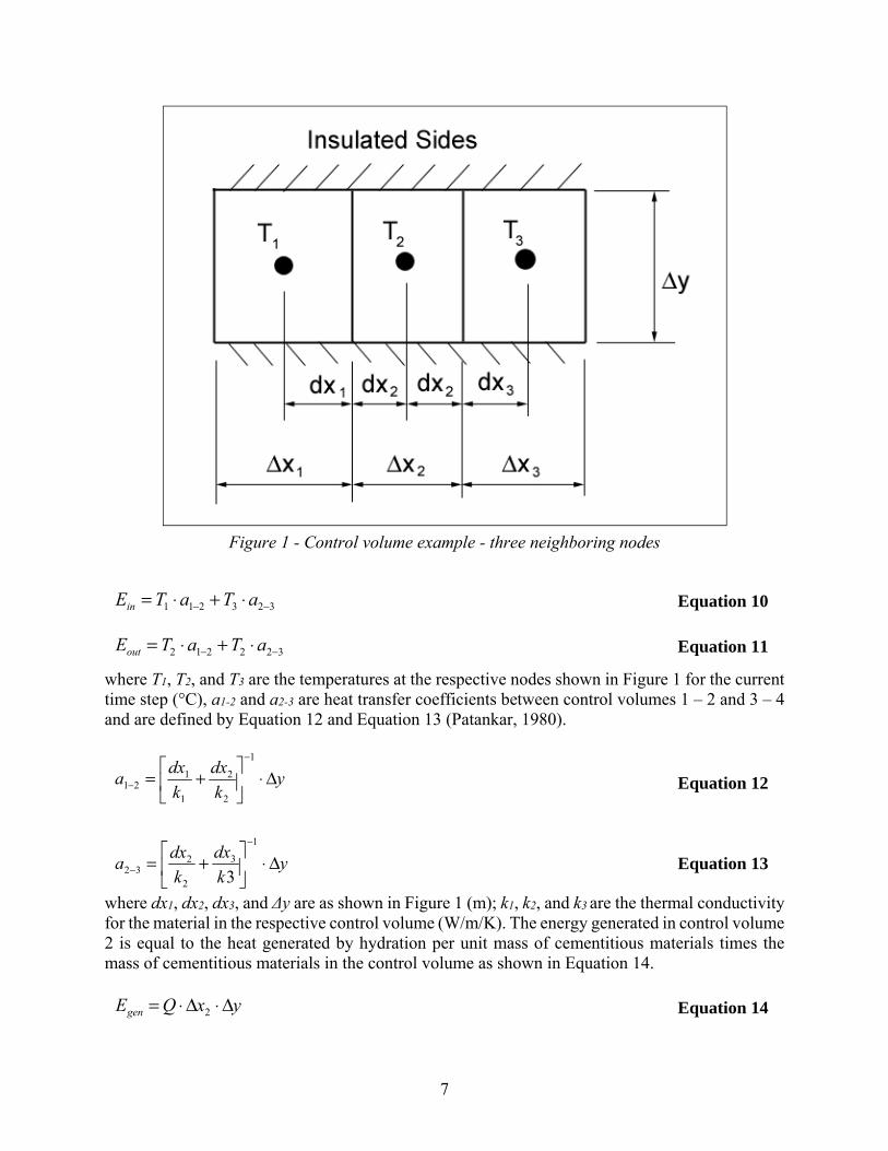
Figure 1 shows three neighboring control volumes with insulated sides. An explicit time discretization has been used in formulating these equations, which is explained in Section 3.1.2. The change in energy entering and leaving the control volume 2 can be calculated using Equation 10 and Equation 11.

7

Figure 1 - Control volume example - three neighboring nodes

323211 −− ⋅+⋅= aTaTEin Equation 10

322212 −− ⋅+⋅= aTaTEout Equation 11

where T1, T2, and T3 are the temperatures at the respective nodes shown in Figure 1 for the current time step (°C), a1-2 and a2-3 are heat transfer coefficients between control volumes 1 – 2 and 3 – 4 and are defined by Equation 12 and Equation 13 (Patankar, 1980).

yk

dx

k

dxa Δ⋅

+=

−

−

1

2

2

1

121 Equation 12

yk

dx

k

dxa Δ⋅

+=

−

−

1

3

2

232 3

Equation 13

where dx1, dx2, dx3, and Δy are as shown in Figure 1 (m); k1, k2, and k3 are the thermal conductivity for the material in the respective control volume (W/m/K). The energy generated in control volume 2 is equal to the heat generated by hydration per unit mass of cementitious materials times the mass of cementitious materials in the control volume as shown in Equation 14.

yxQEgen Δ⋅Δ⋅= 2 Equation 14

8

where Q is the heat generated per unit mass of cementitious materials (W); Δx2 and Δy are as shown in Figure 1 (m). For control volume 2, Q may be calculated based on the Arrhenius equation as shown in Equation 15 (Schindler, 2004):

⋅

+

−+

⋅

−⋅

⋅

⋅⋅=

3600

1

273

1

273

1expexp*)(

2TTR

E

tttCHtQ

r

a

e

u

ee

cue

ββ

ταβτ Equation 15

where te is the concrete equivalent age at the reference temperature as shown in Equation 16 (hrs), Hu is the total amount of heat generated at 100% hydration (J/kg), Cc is the total amount of cementitious materials (kg/m3), τ is the hydration time parameter (hrs), β is the hydration slope parameter, αu is the ultimate degree of hydration, Ea is the activation energy (J/mol), R is the universal gas constant (J/mol/K), and Tr is the reference temperature (°C). The degree of hydration is calculated as shown in Equation 17.

dtTTR

AETt

t

re ⋅

+

−+

⋅= 0 2

2 273

1

273

1exp)( Equation 16

−⋅=

βταα

eue t

t exp)( Equation 17

The change in energy stored in the control volume is shown in Equation 18.

t

TTyxcE p

st Δ−⋅Δ⋅Δ⋅⋅

=Δ+ )( 2

12222ρ

Equation 18

where ρ2 is the material density in control volume 2 (kg/m3), cp2 is the material specific heat in control volume 2 (J/kg/K), T2

+1 is the temperature at node 2 for the next time step (°C), T2 is the temperature at node 2 for the current time step (°C), and Δt is the time step (seconds).

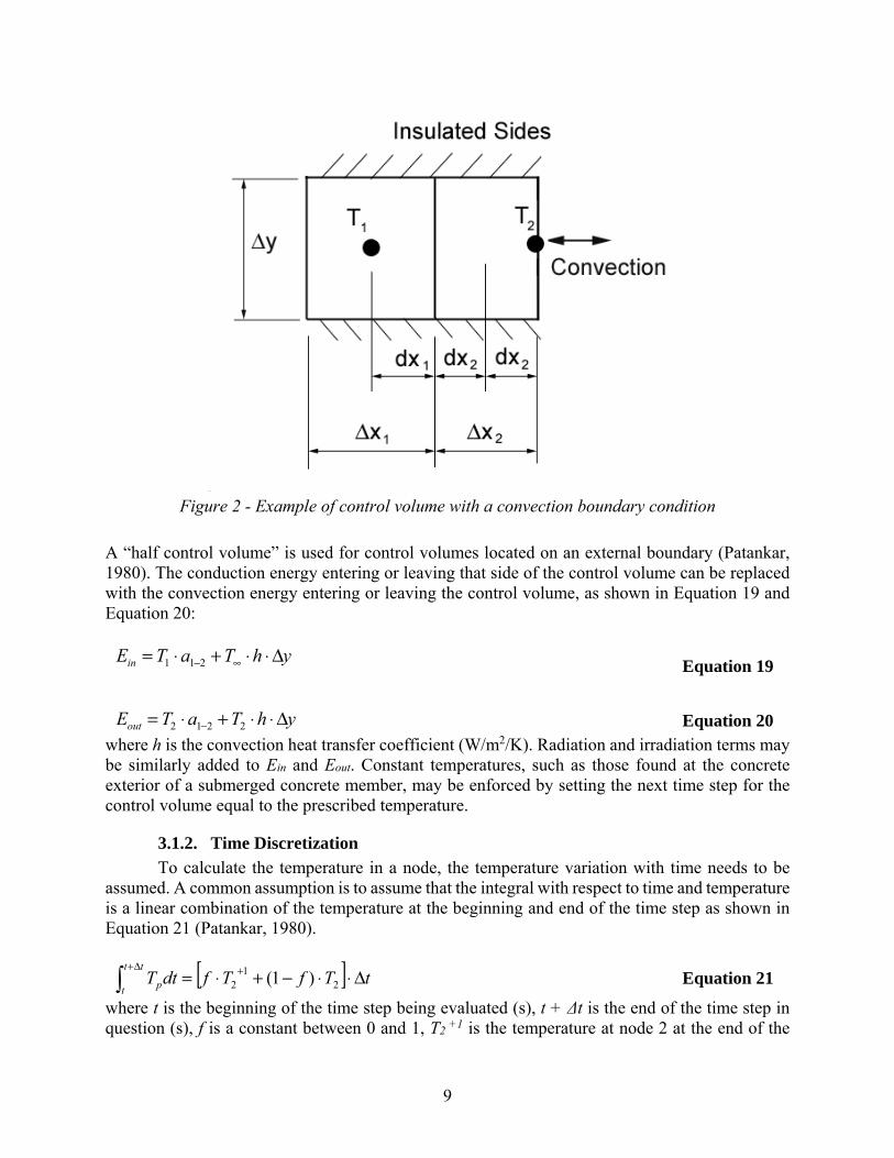
Boundary conditions are easily handled using the energy balance approach. A control volume with a side exposed to convection is shown in Figure 2.

9

Figure 2 - Example of control volume with a convection boundary condition

A “half control volume” is used for control volumes located on an external boundary (Patankar, 1980). The conduction energy entering or leaving that side of the control volume can be replaced with the convection energy entering or leaving the control volume, as shown in Equation 19 and Equation 20:

yhTaTEin Δ⋅⋅+⋅= ∞−211 Equation 19

yhTaTEout Δ⋅⋅+⋅= − 2212 Equation 20where h is the convection heat transfer coefficient (W/m2/K). Radiation and irradiation terms may be similarly added to Ein and Eout. Constant temperatures, such as those found at the concrete exterior of a submerged concrete member, may be enforced by setting the next time step for the control volume equal to the prescribed temperature.

3.1.2. Time Discretization

To calculate the temperature in a node, the temperature variation with time needs to be assumed. A common assumption is to assume that the integral with respect to time and temperature is a linear combination of the temperature at the beginning and end of the time step as shown in Equation 21 (Patankar, 1980).

[ ] tTfTfdtTtt

t p Δ⋅⋅−+⋅= +Δ+

21

2 )1( Equation 21

where t is the beginning of the time step being evaluated (s), t + Δt is the end of the time step in question (s), f is a constant between 0 and 1, T2

+1 is the temperature at node 2 at the end of the

10

time step (°C), and T2 is the temperature at node 2 at the beginning of the time step (°C). When f is chosen to be 0, the time discretization is said to be fully explicit and the temperature during the time step is assumed to be equal to the beginning temperature during the time step. If f is greater than 0, the method is called implicit. If f is assumed to be 1, the method is called fully implicit. The temperature during the time step is then assumed to be equal to the ending temperature during the time step. Explicit methods allow for temperature calculations directly from previous time step temperatures. Implicit methods however, are dependent on unknown temperatures. A system of unknown temperatures must be solved for simultaneously (Patankar, 1980). When the explicit method is used, the temperature at a node for the next time step is completely dependent on the current time step. This means that the unknown temperatures for the next time step do not have to be solved simultaneously.

If care is not taken when fully explicit methods are used, unstable results may be calculated. The stability criterion is shown in Equation 22:

t

TyxcE p

out Δ⋅Δ⋅Δ⋅⋅

< 2222ρ Equation 22

where Eout, ρ2, cp2, Δx2, Δy, T2, and Δt are as defined above. Equation 9 means that the amount of energy leaving the control volume has to be less than the amount of the energy stored in the control volume to give physically possible results. As seen in Equation 22, as the control volume decreases, the time step must also decrease. As a result, explicit finite difference methods can be computationally expensive.

3.1.3. Symmetry

The use of symmetry can significantly decrease the amount of computations needed. At a line of symmetry, the derivative of the temperature profile is zero. This implies that no heat is exchanged across the line of symmetry. The energy leaving and entering the face of the control volume on the line of symmetry is set equal to zero. The assumption of symmetry may lead to some inaccuracies when modeling boundary conditions, such as when one side of a concrete member is shaded and the other is not. If symmetry where not assumed, longer run times would occur and more complex program inputs (including inputs that may not be available to the engineer) would be required.

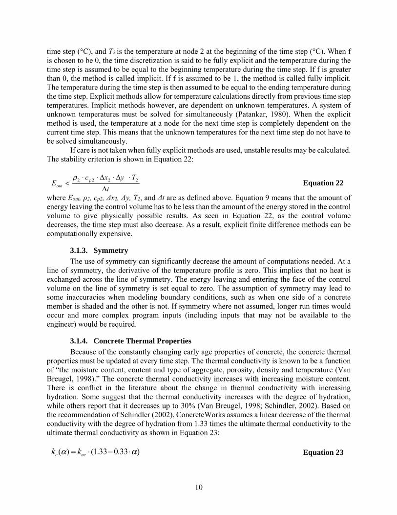
3.1.4. Concrete Thermal Properties

Because of the constantly changing early age properties of concrete, the concrete thermal properties must be updated at every time step. The thermal conductivity is known to be a function of “the moisture content, content and type of aggregate, porosity, density and temperature (Van Breugel, 1998).” The concrete thermal conductivity increases with increasing moisture content. There is conflict in the literature about the change in thermal conductivity with increasing hydration. Some suggest that the thermal conductivity increases with the degree of hydration, while others report that it decreases up to 30% (Van Breugel, 1998; Schindler, 2002). Based on the recommendation of Schindler (2002), ConcreteWorks assumes a linear decrease of the thermal conductivity with the degree of hydration from 1.33 times the ultimate thermal conductivity to the ultimate thermal conductivity as shown in Equation 23:

)33.033.1()( αα ⋅−⋅= ucc kk Equation 23

11

where kc is the concrete thermal conductivity (W/m/K), α is the degree of hydration, and kuc is the ultimate hardened concrete thermal conductivity. The thermal conductivity of the concrete is not adjusted for moisture content in ConcreteWorks because the moisture content in mass concrete does not change significantly during early ages. The thermal conductivity is also not adjusted for temperature because of the differing responses of different aggregates.

The specific heat of concrete is also dependent on the mixture proportions, degree of hydration, temperature, and moisture level (Van Breugel, 1998; Schindler, 2002). A model proposed by Van Breugel accounts for changes in the specific heat based on degree of hydration, mixture proportions, and temperature as shown in Equation 24:

))1((1

wwaacccefcconc

pconc cWcWcWcWc ⋅+⋅+⋅−⋅+⋅⋅⋅= ααρ

Equation 24

where cpconc is the specific heat of the concrete (J/kg/K), ρconc is the concrete density (kg/m3), Wc is the weight of cement (kg/m3), Wa is the weight of aggregate (kg/m3), Ww is the weight of water (kg/m3), Cc is the cement specific heat (J/kg/K), Ca is the aggregate specific heat (J/kg/K), Cw is the water specific heat (J/kg/k), and Ccef is a fictitious specific heat of the hydrating cement as shown in Equation 25:

3394.8 +⋅= cref Tc Equation 25

where Tc is the concrete temperature (°C).

3.1.5. Concrete Heat of Hydration

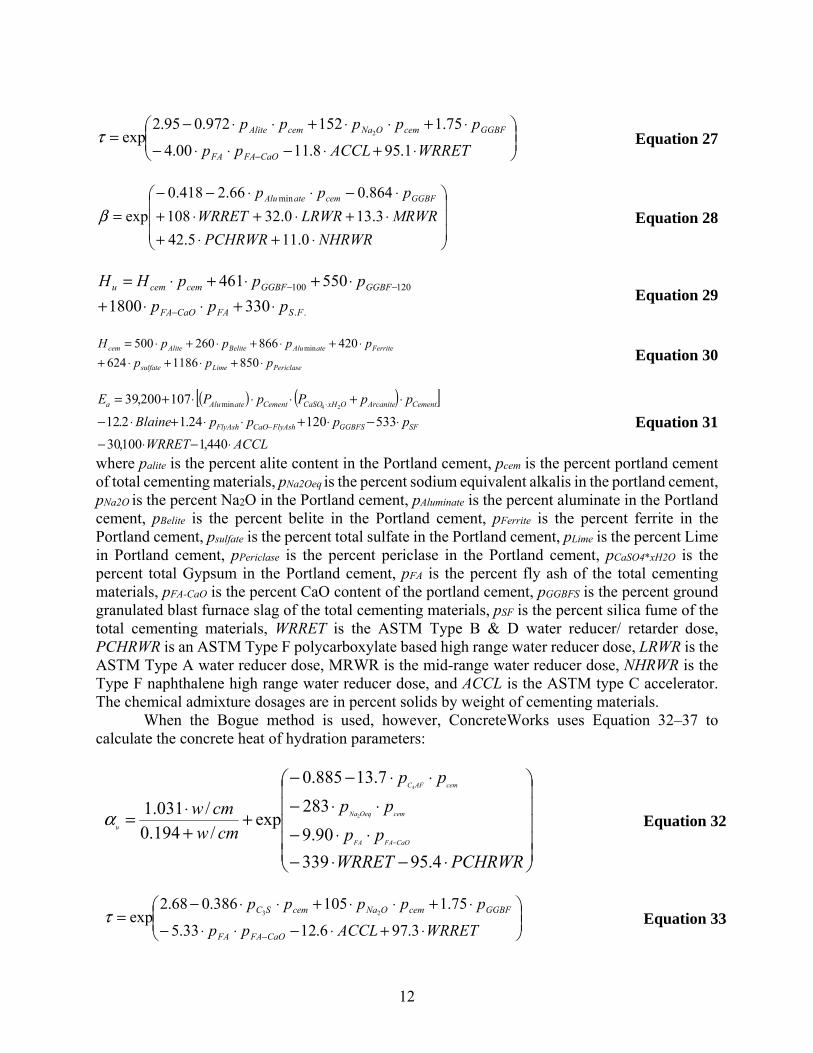
The concrete heat of hydration parameters Hu, τ, β, αu, and Ea can be calculated based on the concrete mixture proportions and constituent material properties. The τ, β, αu parameters are calculated from a statistical analysis developed based on over 300 semi-adiabatic calorimetry tests performed according to recommendations from the RILEM technical committee 119 (1998) and validated by 18 tests conducted on concrete sampled from concrete construction sites and 44 tests conducted independently by Schindler and Folliard (2005) and Ge (2006). The dataset used includes concrete containing various chemical admixtures, cement fineness and chemical composition, and supplementary cementing materials on the heat of hydration. The apparent activation energy Ea can also be calculated based on the cementing material properties and the chemical admixtures used. A statistical analysis of 117 apparent activation energies calculated from isothermal calorimetry was developed by Poole (2007). The Hu parameter can also be calculated from the cement chemical composition using a model developed by Schindler and later altered to better characterize the influence of grade 120 ground granulated blast furnace slag by Poole (2007). The cement composition can be defined in ConcreteWorks using either the Rietveld method (Rietveld, 1969) determined from quantitative x-ray diffraction or the Bogue method calculated according to ASTM C 150 (2005). When the Rietveld method is used to determine the cement chemical composition, Equation 26–31 are used in ConcreteWorks to calculate the concrete heat of hydration parameters:

⋅−⋅−⋅⋅−

⋅⋅−⋅⋅−−

++⋅=

−

PCHRWRWRRET

pp

pp

pp

cmw

cmw

CaOFAFA

cemOeqNa

cemFerrite

u

8.93331

90.8

325

73.9297.0

exp/194.0

/031.1 2α

Equation 26

12

⋅+⋅−⋅⋅−

⋅+⋅⋅+⋅⋅−=

− WRRETACCLpp

ppppp

CaOFAFA

GGBFcemONacemAlite

1.958.1100.4

75.1152972.095.2exp 2τ Equation 27

⋅+⋅+⋅+⋅+⋅+

⋅−⋅⋅−−=

NHRWRPCHRWR

MRWRLRWRWRRET

ppp GGBFcemateAlu

0.115.42

3.130.32108

864.066.2418.0

expmin

β Equation 28

..

120100

3301800

550461

FSFACaOFA

GGBFGGBFcemcemu

ppp

pppHH

⋅+⋅⋅+⋅+⋅+⋅=

−

−− Equation 29

PericlaseLimesulfate

FerriteateAluBeliteAlitecem

ppp

ppppH

⋅+⋅+⋅+⋅+⋅+⋅+⋅=

8501186624

420866260500 min Equation 30

( ) ( )[ ]

ACCLWRRET

ppppBlaine

ppPpPE

SFGGBFSFlyAshCaOFlyAsh

CementArcaniteOxHCaSOCementateAlua

⋅−⋅−

⋅−⋅+⋅⋅+⋅−

⋅+⋅⋅⋅+=

−

⋅

440,1100,30

53312024.12.12

107200,3924min

Equation 31

where palite is the percent alite content in the Portland cement, pcem is the percent portland cement of total cementing materials, pNa2Oeq is the percent sodium equivalent alkalis in the portland cement, pNa2O is the percent Na2O in the Portland cement, pAluminate is the percent aluminate in the Portland cement, pBelite is the percent belite in the Portland cement, pFerrite is the percent ferrite in the Portland cement, psulfate is the percent total sulfate in the Portland cement, pLime is the percent Lime in Portland cement, pPericlase is the percent periclase in the Portland cement, pCaSO4*xH2O is the percent total Gypsum in the Portland cement, pFA is the percent fly ash of the total cementing materials, pFA-CaO is the percent CaO content of the portland cement, pGGBFS is the percent ground granulated blast furnace slag of the total cementing materials, pSF is the percent silica fume of the total cementing materials, WRRET is the ASTM Type B & D water reducer/ retarder dose, PCHRWR is an ASTM Type F polycarboxylate based high range water reducer dose, LRWR is the ASTM Type A water reducer dose, MRWR is the mid-range water reducer dose, NHRWR is the Type F naphthalene high range water reducer dose, and ACCL is the ASTM type C accelerator. The chemical admixture dosages are in percent solids by weight of cementing materials.

When the Bogue method is used, however, ConcreteWorks uses Equation 32–37 to calculate the concrete heat of hydration parameters:

⋅−⋅−⋅⋅−

⋅⋅−⋅⋅−−

++⋅=

−

PCHRWRWRRET

pp

pp

pp

cmwcmw

CaOFAFA

cemOeqNa

cemAFC

u

4.95339

90.9

283

7.13885.0

exp/194.0

/031.12

4

α

Equation 32

⋅+⋅−⋅⋅−

⋅+⋅⋅+⋅⋅−=

− WRRETACCLpp

ppppp

CaOFAFA

GGBFcemONacemSC

3.976.1233.5

75.1105386.068.2exp 23τ Equation 33

13

⋅+⋅+⋅+⋅+⋅+

⋅−⋅⋅−−

=NHRWRPCHRWR

MRWRLRWRWRRET

ppp GGBFcemAC

07.93.38

2.234.398.96

594.080.3494.0

exp3

β Equation 34

..

120100

3301800

550461

FSFACaOFA

GGBFGGBFcemcemu

ppp

pppHH

⋅+⋅⋅+⋅+⋅+⋅=

−

−− Equation 35

MgOFreeCaSO

AFCACSCSCcem

ppp

ppppH

⋅+⋅+⋅+

⋅+⋅+⋅+⋅=

8501186624

420866260500

3

4323 Equation 36

( )[ ]

ACCLWRRET

pppp

BlaineONa

pGypsumpAFCACE

SFGGBFSFlyAshCaOFlyAsh

eq

CementCementa

⋅−⋅−

⋅−⋅+⋅⋅+

⋅−⋅−⋅⋅⋅+⋅+=

−

450,1900,30

51616296.2

8.19470,3

330,8230,41

2

43

Equation 37

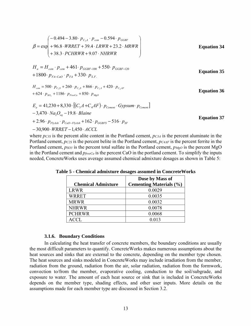
where pC3S is the percent alite content in the Portland cement, pC3A is the percent aluminate in the Portland cement, pC2S is the percent belite in the Portland cement, pC4AF is the percent ferrite in the Portland cement, pSO3 is the percent total sulfate in the Portland cement, pMgO is the percent MgO in the Portland cement and pfreeCa is the percent CaO in the portland cement. To simplify the inputs needed, ConcreteWorks uses average assumed chemical admixture dosages as shown in Table 5:

Table 5 - Chemical admixture dosages assumed in ConcreteWorks

Chemical Admixture Dose by Mass of

Cementing Materials (%) LRWR 0.0029 WRRET 0.0035 MRWR 0.0032 NHRWR 0.0078 PCHRWR 0.0068 ACCL 0.013

3.1.6. Boundary Conditions

In calculating the heat transfer of concrete members, the boundary conditions are usually the most difficult parameters to quantify. ConcreteWorks makes numerous assumptions about the heat sources and sinks that are external to the concrete, depending on the member type chosen. The heat sources and sinks modeled in ConcreteWorks may include irradiation from the member, radiation from the ground, radiation from the air, solar radiation, radiation from the formwork, convection to/from the member, evaporative cooling, conduction to the soil/subgrade, and exposure to water. The amount of each heat source or sink that is included in ConcreteWorks depends on the member type, shading effects, and other user inputs. More details on the assumptions made for each member type are discussed in Section 3.2.

14

Modeling each type of heat source or sink in ConcreteWorks requires numerous equations. Details about many of the boundary conditions equations used in ConcreteWorks, especially for vertical members may be found in the paper “Temperature Boundary Condition Models for Concrete Bridge Members” (Riding et al., 2007). The evaporative cooling model is from Schindler (2002). It combines models from the ASHRAE handbook (1993) and Al-Fadhala and Hover (2001) to predict the evaporation and consequently the cooling rate for concrete surfaces. The model is based on the work of Menzel that applied water evaporation rate equations developed by Koehler to concrete. The evaporation rate follows Dalton’s law, which relates the water-vapor pressure of the air, at the water surface, and the wind speed (which helps speed up evaporation) to the evaporation rate (Hover, 2006). Menzel’s equation is shown as Equation 38 (Al-Fadhala and Hover, 2001):

)060.0253.0)((315.0 0 weRHeE aw +⋅−= Equation 38

where Ew is the water evaporation rate (kg/m2/hr), e0 is the water surface saturated water vapor pressure (mmHg), ea is the air water vapor pressure (mmHg), RH is the relative humidity (as a decimal), and w is the wind speed (m/s). The terms e0 and ea are dependent on the water surface and air temperatures. Concrete follows Dalton’s law pretty well when bleed water is on the surface, and decreases rapidly during setting. The amount of evaporation from concrete may be related to the amount of evaporation from a water surface by Equation 39 (Al-Fadhala and Hover, 2001):

−=

5.1

expevapw

c

a

t

E

E Equation 39

where Ec is the evaporation rate from concrete (kg/m2/hr), t is the time from mixing (hrs), and aevap is mixture dependent time constant (hrs). ConcreteWorks assumes that aevap is equal to 3.75 hours. The evaporative cooling model is applied until either a cure method is applied or 24 hours after placing.

3.2. Concrete Member Models

Each type of concrete member modeled in ConcreteWorks has different formwork, boundary conditions, geometry, and opportunities to use symmetry. Different nodal arrangements are also required to keep nodes in a regular pattern and in line.

3.2.1. Rectangular Column

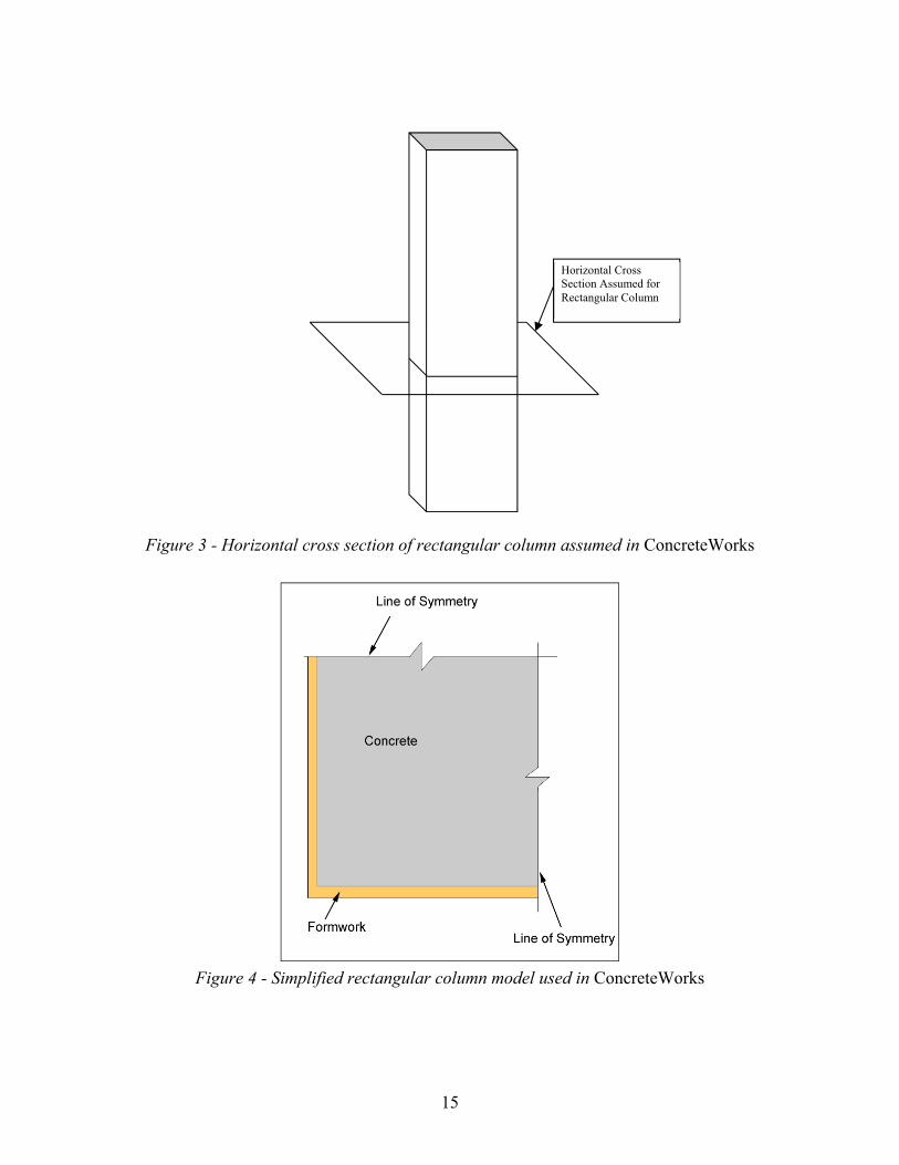
ConcreteWorks models a two-dimensional horizontal cross section for rectangular columns, as shown in Figure 3. The column heat transfer in the vertical direction is assumed to be zero, which is a reasonable assumption except near the top and bottom ends of the column. Rectangular columns are modeled using symmetry in both directions as shown in Figure 4. The formwork is handled by using half control volumes around the concrete, as shown in Figure 5. ConcreteWorks allows the user to select up to three construction stages to model for rectangular columns by selecting different formwork removal times and curing techniques.

15

Figure 3 - Horizontal cross section of rectangular column assumed in ConcreteWorks

Figure 4 - Simplified rectangular column model used in ConcreteWorks

Horizontal Cross Section Assumed for Rectangular Column

16

Figure 5 - Example rectangular column node and control volumes

The first construction stage is during concrete placement and curing before form removal. When steel formwork is selected and form-liners are not selected, ConcreteWorks assumes that the steel provides no insulation because of the “little resistance to heat dissipation from the concrete” (ACI 207.2, 1995). The steel emissivity, absorptivity, and shading values are then assigned to the concrete surface node, so that the surface of the column will still see the same heating from the environment. Eliminating the form control volumes for steel formwork greatly increases the runtime because of the small time step needed to maintain stability with such a thin control volume needed to model a steel form. When form-liners are used, ConcreteWorks calculates an equivalent form thermal conductivity, density, and specific heat for the selected combination of form and form-liner. The thermal conductivity, density, and specific heat of the equivalent form are calculated using Equation 40–42:

1−

+=

fl

fl

f

fef k

w

k

wk Equation 40

flf

flflffef ww

ww

+⋅+⋅

=ρρ

ρ Equation 41

flf

flflffef cpcp

wcpwcpcp

+⋅+⋅

= Equation 42

where kef is the effective form thermal conductivity (W/m/K), wf is the width of the form (m), wfl is the width of the form-liner (m), kf is the form thermal conductivity (W/m/K), kfl is the form-liner thermal conductivity (W/m/K), ρef is the effective form density (kg/m3), ρf is the form density (kg/m3), ρfl is the form-liner density (kg/m3), cpef is the effective form specific heat (J/kg/K), cpf is

17

the form specific heat (J/kg/K), and cpef is the form-liner specific heat (J/kg/K). In ConcreteWorks, form-liners are assumed to have a thickness of 0.036 m (1.4 in), a thermal conductivity of 0.7437 W/m/°C, a specific heat of 1549.1 J/kg/K, and a density of 1121 kg/m3.

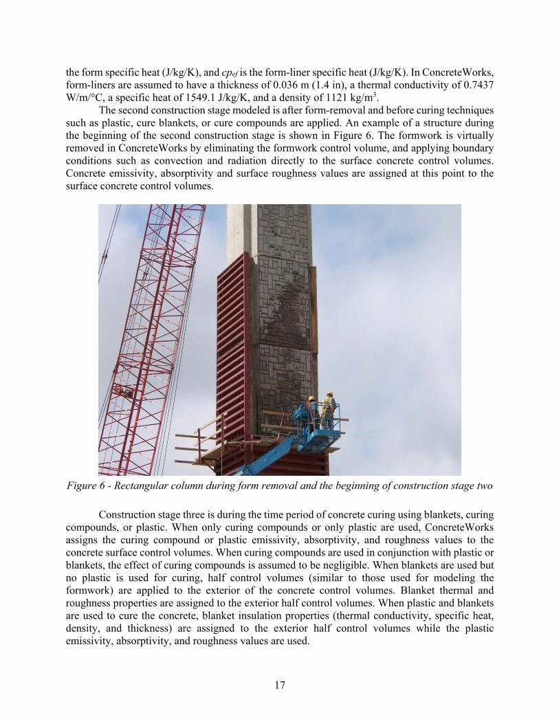
The second construction stage modeled is after form-removal and before curing techniques such as plastic, cure blankets, or cure compounds are applied. An example of a structure during the beginning of the second construction stage is shown in Figure 6. The formwork is virtually removed in ConcreteWorks by eliminating the formwork control volume, and applying boundary conditions such as convection and radiation directly to the surface concrete control volumes. Concrete emissivity, absorptivity and surface roughness values are assigned at this point to the surface concrete control volumes.

Figure 6 - Rectangular column during form removal and the beginning of construction stage two

Construction stage three is during the time period of concrete curing using blankets, curing compounds, or plastic. When only curing compounds or only plastic are used, ConcreteWorks assigns the curing compound or plastic emissivity, absorptivity, and roughness values to the concrete surface control volumes. When curing compounds are used in conjunction with plastic or blankets, the effect of curing compounds is assumed to be negligible. When blankets are used but no plastic is used for curing, half control volumes (similar to those used for modeling the formwork) are applied to the exterior of the concrete control volumes. Blanket thermal and roughness properties are assigned to the exterior half control volumes. When plastic and blankets are used to cure the concrete, blanket insulation properties (thermal conductivity, specific heat, density, and thickness) are assigned to the exterior half control volumes while the plastic emissivity, absorptivity, and roughness values are used.

18

Blanket insulation properties are calculated from the blanket R-value entered by the user. The R-value is equivalent to the thickness divided by the thermal conductivity. ConcreteWorks assumes a blanket thickness of 0.02 m and then solves for the blanket thermal conductivity kbl (W/m/K) as shown in Equation 43:

blbl R

k02.0= Equation 43

where Rbl is the blanket R-value (m2K/W). The specific heat of the wet blanket is assumed to be 320 kg/m3 while the specific heat is assumed to be 2000 J/kg/K.

3.2.2. Rectangular Footing

Footings have some unique features that require special cases for modeling. When footings are modeled in two dimensions, ConcreteWorks assumes a vertical cross section of the footing as shown in Figure 7 with no heat transfer perpendicular to the cross section. The heat exchange between the footing and the environment is dependent on the formwork, cure blankets and plastic used, soil conditions, weather, orientation of the footing, shading from scaffolding and embankments, and heat conduction from the concrete interior. Figure 8 summarizes the footing surface boundary conditions.

Figure 7 - Diagram of the vertical cross section assumed in modeling a two-dimensional footing

Vertical cross section modeled in 2-d footing

19

Figure 8 - Summary of rectangular footing boundary conditions

Radiation

Solar Radiation, atmospheric radiation, irradiation from the footing, and the radiation exchange between the vertical surface and form horizontal cross bracing models are used in the side and top boundary condition calculations. Radiation emitted by the ground surface is assumed to be incident on the side surface only. If the user chooses to shade the sides of the footing because of scaffolding or the embankment, then the solar radiation is set to zero.

Conduction to/from Soil

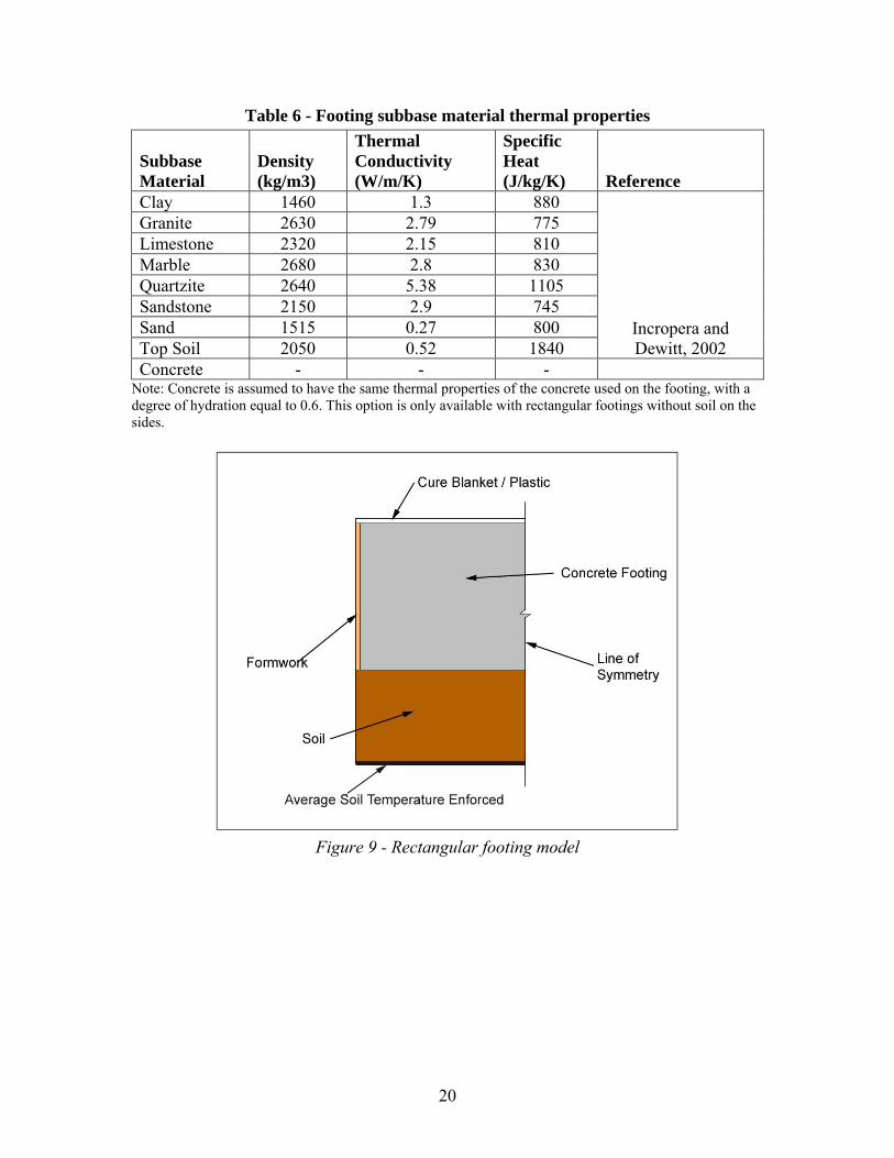
Conduction to/from the soil underneath the footing is modeled by assuming a constant depth of soil. The initial temperature of the soil is set to the user defined average soil temperature. The temperature at the bottom of the modeled soil is set also set to the user defined average soil temperature. Table 6 lists the thermal properties of the different soil and rock types modeled by ConcreteWorks. Figure 9 shows how the rectangular footing is modeled, and Figure 10 illustrates the node and control volume boundaries assumed. Symmetry is assumed in the model in the width and length (when calculated in three dimensions) direction as shown in the figure.

20

Table 6 - Footing subbase material thermal properties

Subbase Material

Density (kg/m3)

Thermal Conductivity (W/m/K)

Specific Heat (J/kg/K) Reference

Clay 1460 1.3 880

Incropera and Dewitt, 2002

Granite 2630 2.79 775 Limestone 2320 2.15 810 Marble 2680 2.8 830 Quartzite 2640 5.38 1105 Sandstone 2150 2.9 745 Sand 1515 0.27 800 Top Soil 2050 0.52 1840 Concrete - - -

Note: Concrete is assumed to have the same thermal properties of the concrete used on the footing, with a degree of hydration equal to 0.6. This option is only available with rectangular footings without soil on the sides.

Figure 9 - Rectangular footing model

21

Figure 10 - Node layout for rectangular footing

Construction Stages

Rectangular footings can modeled with up to four potential construction stages. The first stage is before the blanket or any cure method is applied to the top surface. The second stage is when the cure method is applied to the top surface. ConcreteWorks assumes that a cure blanket is placed on the top surface when the cure method is applied. Any other cure methods such as plastic will also be placed and will affect the absorptivity and emissivity of the top cure surface. The third stage is after form and cure method removal. The fourth construction stage represents the time period when a cure method on the top and sides is used after the forms and initial top surface curing methods are removed. If a cure blanket is selected for this stage, it is applied uniformly over the top and side surfaces.

3.2.3. Rectangular Footing with Soil on the Sides

ConcreteWorks contains an option for soil to be used as the formwork, as shown in Figure 11. Symmetry is assumed in the middle of the member as shown. Conduction to/from the soil on the sides is treated in a similar manner to the soil underneath the footing. A constant thickness of soil is modeled on the sides of the footing. The average soil temperature is enforced on the sides at the edge of the soil, as shown in Figure 12. The node and control volume layout for the rectangular footing with soil on the sides is shown in Figure 13.

22

Figure 11 - Summary of rectangular footing with soil on the sides

Figure 12 - Rectangular footing with “soil on sides” model

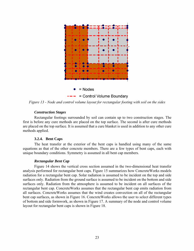
23

Figure 13 - Node and control volume layout for rectangular footing with soil on the sides

Construction Stages

Rectangular footings surrounded by soil can contain up to two construction stages. The first is before any cure methods are placed on the top surface. The second is after cure methods are placed on the top surface. It is assumed that a cure blanket is used in addition to any other cure methods applied.

3.2.4. Bent Caps

The heat transfer at the exterior of the bent caps is handled using many of the same equations as that of the other concrete members. There are a few types of bent caps, each with unique boundary conditions. Symmetry is assumed in all bent cap members.

Rectangular Bent Cap

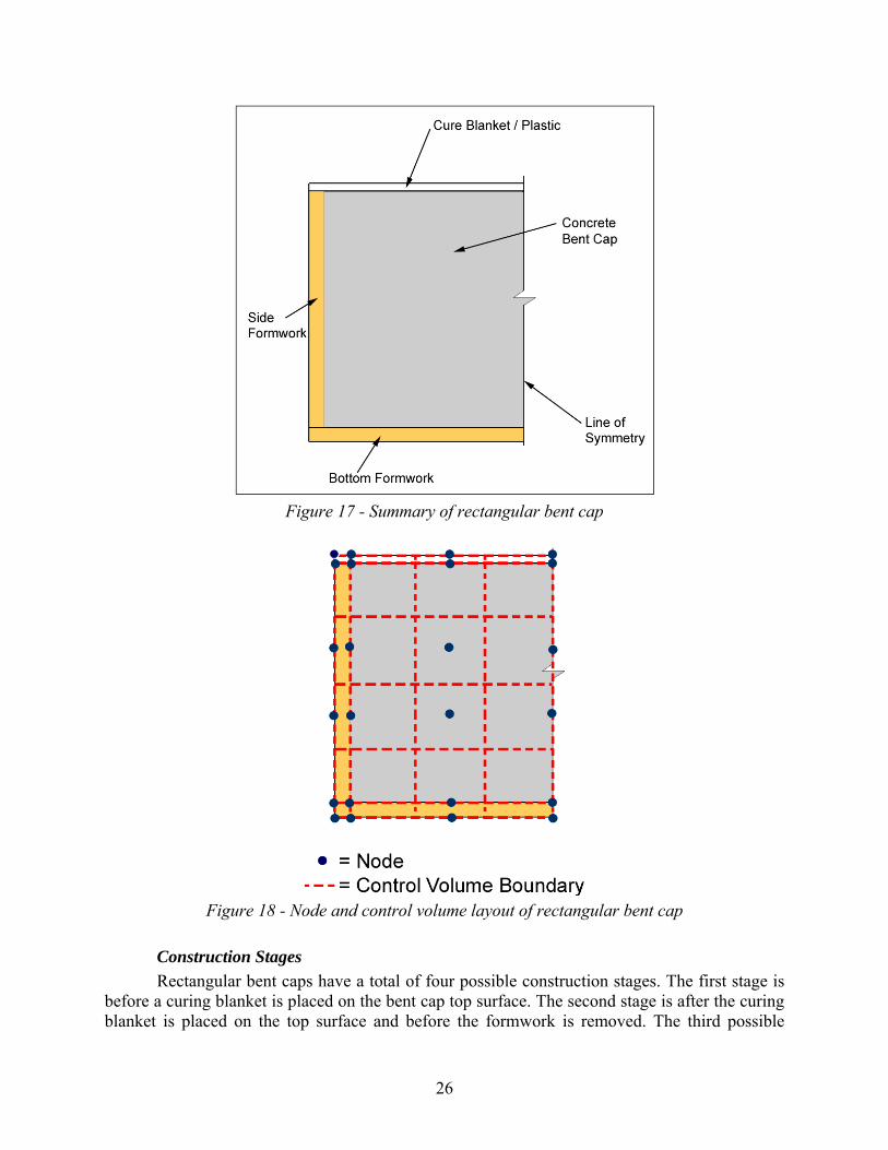
Figure 14 shows the vertical cross section assumed in the two-dimensional heat transfer analysis performed for rectangular bent caps. Figure 15 summarizes how ConcreteWorks models radiation for a rectangular bent cap. Solar radiation is assumed to be incident on the top and side surfaces only. Radiation from the ground surface is assumed to be incident on the bottom and side surfaces only. Radiation from the atmosphere is assumed to be incident on all surfaces of the rectangular bent cap. ConcreteWorks assumes that the rectangular bent cap emits radiation from all surfaces. ConcreteWorks assumes that the wind creates convection on all of the rectangular bent cap surfaces, as shown in Figure 16. ConcreteWorks allows the user to select different types of bottom and side formwork, as shown in Figure 17. A summary of the node and control volume layout for rectangular bent caps is shown in Figure 18.

24

Figure 14 - Diagram of the vertical cross section modeled in a rectangular bent cap

Figure 15 - Rectangular bent cap radiation summary

Vertical cross section modeled in 2-d rectangular bent cap

25

Figure 16 - Rectangular bent cap convection summary

26

Figure 17 - Summary of rectangular bent cap

Figure 18 - Node and control volume layout of rectangular bent cap

Construction Stages

Rectangular bent caps have a total of four possible construction stages. The first stage is before a curing blanket is placed on the bent cap top surface. The second stage is after the curing blanket is placed on the top surface and before the formwork is removed. The third possible

27

construction stage is after the formwork and curing blanket is removed. The last possible construction stage is after a curing blanket is wrapped around the bent cap.

Dolphin

ConcreteWorks allows the user to select pre-cast concrete as the bottom formwork material. Pre-cast concrete is assumed to have the same material thermal properties as the concrete mixture used for the bent cap with a degree of hydration equal to 0.6. When the user inputs that the bent cap is a dolphin, the temperature of the bottom of the bent cap is set equal to the average water temperature. Figure 19 shows a summary of a dolphin with a pre-cast concrete bottom.

Figure 19 - Summary of dolphin with pre-cast concrete bottom

3.2.5. T-Shaped Bent Cap

The T-shaped bent cap modeled in ConcreteWorks assumes the same type of vertical cross section as the rectangular bent cap. Figure 20 shows a summary of how ConcreteWorks models radiation boundary conditions in T-shaped bent caps. Radiation from the ground surface is assumed to be incident on the cap bottom and sides. Solar Radiation is assumed to be incident on all the top of the cap, the top of the corbel, and the sides. Radiation from the atmosphere is assumed to be incident on all sides. The cap is assumed to emit radiation from all surfaces. ConcreteWorks assumes that the wind creates convection on all of the T-shaped bent cap surfaces, as shown in Figure 21. ConcreteWorks allows the user to select different types of bottom and side formwork, as shown in Figure 22. The node and control volume layout for the T-shaped bent cap is shown in Figure 23.

28

Figure 20 - Summary of radiation boundary conditions for T-shaped bent caps

Figure 21 - Summary of convection boundary conditions on T-shaped bent cap

29

Figure 22 - Construction summary form T-shaped bent cap

Figure 23 - Node and control volume layout for T-shaped bent caps

Construction Stages

T-shaped bent caps use the same construction stages as rectangular bent caps.

30

3.2.6. Circular Columns

ConcreteWorks models a horizontal cross section of the circular column, just like that of a rectangular column. The boundary conditions for both rectangular and circular columns are handled in a similar manner. Circular columns are modeled in ConcreteWorks using the same radiation and convection boundary conditions as rectangular columns. Figure 24 shows a summary of the construction model used for a circular column in ConcreteWorks. Symmetry is assumed in the circumferential direction. Figure 25 shows the node and control volume layout for a circular column. Figure 26 shows the boundary conditions modeled for circular columns. ConcreteWorks applies convection on the outer surface of the model of the circular column. Radiation from ground surfaces, atmospheric radiation, solar radiation, and irradiation are also modeled on the outer surface of the column.

Figure 24 - Circular column model

31

Figure 25 - Node and control volume layout for circular columns

Figure 26 - Circular column boundary conditions

Construction Stages

Circular columns use the same construction stages as rectangular columns.

3.2.7. Bridge Decks

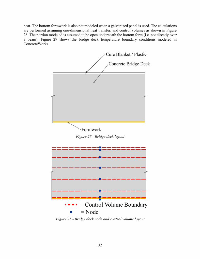
The fundamental heat transfer calculations performed for all four types of bridge decks modeled in ConcreteWorks are the same. Figure 27 shows the basic layout of the bridge deck modeled. In the case of a bridge deck with a precast panel, no bottom form is modeled. The precast panel thermal conductivity and specific heat properties are calculated using Equation 23 and Equation 24, with a degree of hydration equal to 0.6. The precast panel is assumed to generate no

32

heat. The bottom formwork is also not modeled when a galvanized panel is used. The calculations are performed assuming one-dimensional heat transfer, and control volumes as shown in Figure 28. The portion modeled is assumed to be open underneath the bottom form (i.e. not directly over a beam). Figure 29 shows the bridge deck temperature boundary conditions modeled in ConcreteWorks.

Figure 27 - Bridge deck layout

Figure 28 - Bridge deck node and control volume layout

33

Figure 29 - Bridge deck temperature boundary conditions

Construction Stages

Bridge decks have up to four possible construction stages. The first is before the cure method is applied to the top surface. A cure blanket is assumed to be used along with any additional curing methods selected by the user. The second stage is after the cure blanket is placed on the top surface, but before form removal and cure method removal. There are two possible final construction stages. An optional third construction stage is when the formwork remains on, but the cure method is removed from the top surface. The fourth construction stage in this option is when the form has been removed following the blanket removal. In the second option, the third construction stage is when the formwork is removed before the cure method is removed from top. Option two’s fourth construction stage is when the cure method is removed after the bottom formwork removal.

3.2.8. Precast Rectangular and U-Shaped Beams

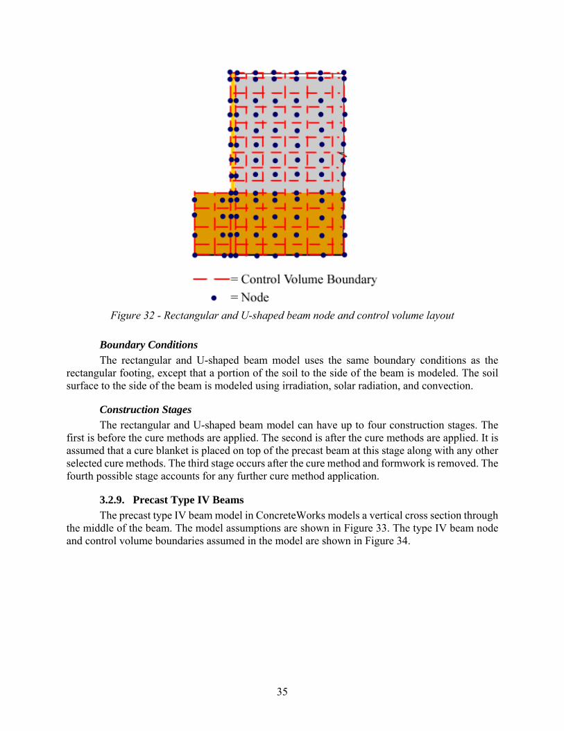
Precast rectangular and U-shaped beams are handled in the same way in ConcreteWorks. Only the dimensions and number of nodes are changed, depending on which member is selected. ConcreteWorks only models a vertical cross section of the solid beam end block, as shown in Figure 30. Only the end block is modeled to greatly simplify the analysis, and to capture the maximum temperature in the beam, which occurs in the solid end region. Figure 31 shows how the end region concrete, formwork, and soil underneath are modeled in ConcreteWorks. Figure 32 shows the node and control volume layout for the rectangular and U-shaped precast beams.

34

Figure 30 - Modeled region of rectangular and U-shaped beams

Figure 31 - ConcreteWorks simplified model for rectangular and U-shaped beams

35

Figure 32 - Rectangular and U-shaped beam node and control volume layout

Boundary Conditions

The rectangular and U-shaped beam model uses the same boundary conditions as the rectangular footing, except that a portion of the soil to the side of the beam is modeled. The soil surface to the side of the beam is modeled using irradiation, solar radiation, and convection.

Construction Stages

The rectangular and U-shaped beam model can have up to four construction stages. The first is before the cure methods are applied. The second is after the cure methods are applied. It is assumed that a cure blanket is placed on top of the precast beam at this stage along with any other selected cure methods. The third stage occurs after the cure method and formwork is removed. The fourth possible stage accounts for any further cure method application.

3.2.9. Precast Type IV Beams

The precast type IV beam model in ConcreteWorks models a vertical cross section through the middle of the beam. The model assumptions are shown in Figure 33. The type IV beam node and control volume boundaries assumed in the model are shown in Figure 34.

36

Figure 33 - Precast type IV beam model assumed in ConcreteWorks

Figure 34 - Precast type IV beam node and control volume boundary layout

Boundary Conditions

The precast type IV beam top and side boundary conditions include solar radiation, irradiation, radiation from the air, and convection. In addition to conduction from the bottom of

37

the member to the soil, convection is also allowed to occur because of a small gap of air that exists between the member bottom form and the ground underneath. Because the gap is not sealed, convection may occur resulting in cooling.

Construction Stages

The precast type IV beam utilizes the same construction stages as the rectangular precast beam.

3.2.10. Pavements

Pavements are modeled assuming one-dimensional heat transfer in the vertical direction. Figure 35 shows the pavement layers modeled in ConcreteWorks. The thermal conductivities, specific heat, and density values used for the pavement subgrade depends on the user inputs, according to Table 6.

Figure 35 - Pavement layers modeled

38

Figure 36 - Pavement node and control volume boundary layout

Boundary Conditions

The top surface of the pavement is exposed to the same boundary conditions as the bridge deck top surface. The pavement may be cured with a monomolecular compound, a single coat of curing compound, a double coat of curing compound, a clear or black plastic sheet, or a cure blanket. If a monomolecular compound or a curing compound is used, then the user may enter the concrete color after the cure method application. The cure method color will change the concrete surface emissivity and absorptivity. Darker colors (like black and dark gray) have higher solar absorptivity and emissivity values than lighter colors (like white or light gray). The pavement layered system provides conduction to the supporting subbase layers and to the subgrade. ConcreteWorks models 49.2 ft (15 meter) of subbase. The temperature of the bottom of the subbase is modeled using the deep ground water temperature calculated using Equation 44 (Yoshitake, Nagai, Tanimoto, and Hamada 2002):

7.383.0 +⋅= aatgw TT Equation 44where Tgw is the deep ground water temperature (°C), and Taat is the average annual temperature (°C). The average annual temperature in ConcreteWorks is calculated from the weather data entered for the city selected. The soil about 0.6 m below the ground surface remains at a fairly constant temperature throughout the year (Yoshitake, Nagai, Tanimoto, and Hamada 2002). The initial subbgrade and subbase temperature profile used in the analysis is then calculated using the Barber model. The Barber model can estimate the subbase and subgrade temperature profile based on the weather data selected in ConcreteWorks, as shown in Equation 45–51 (Barber 1957, Schindler 2002):

+−⋅−⋅⋅

++⋅−⋅⋅+=

CHC

CztCCHCzH

TTzTVM

arctan262.0sin)(

)exp()(

22

Equation 45

39

( )L0.04985.0 ⋅+⋅=AM

TT for T≥TA Equation 46

( )L0.0498278.05.0 ⋅⋅+⋅=Am

TT for T<TA

( )L0.049867.15.0 ⋅⋅+⋅=RV

TT for T≥TA Equation 47

RVTT ⋅= 5.0 for T<TA

⋅+=k

wH

75.013.11.4 Equation 48

⋅=

ρpc

kC Equation 49

where T(z) is the soil temperature (°C) at depth z (m), TM is the mean effective air temperature (°C) as calculated in Equation 46, TA is the mean air temperature (°C), L is the solar radiation (W/m2), TV is the maximum variation in temperature from the mean (°C) calculated using Equation 47, TR is the maximum daily temperature minus the minimum daily temperature (°C), H is calculated using Equation 48, w is the wind speed (m/s), k is the soil thermal conductivity (W/m2), C is the soil thermal diffusivity calculated using Equation 49 (m2/s), cp is the soil specific heat (J/kg/°C), ρ is the soil density (kg/m3), and t is the time from the beginning of the temperature cycle (hours). The finite difference model excluding the concrete is then run from midnight of the placement date to the placement time to further improve the initial soil temperature profile. The thermal conductivity, specific heat, density, solar absorptivity, and emissivity values assumed for different subbase materials is shown in Table 7:

Table 7 - Pavement subbase material properties

Material Thermal Conductivity (W/m2)

Specific Heat (J/kg/°C)

Density (kg/m3)

Solar Absorptivity

Emissivity

Asphalt Concrete 1.38 1047 2302 0.93 0.93 Cement Stabilized Base 0.985 985 2101 0.65 0.9 Asphalt Stabilized Base 0.865 1025 2002 0.9 0.9 Granular Base 1.59 1214 2066 0.8 0.9 Existing Concrete 2.7 921 2403 0.55 0.92

Construction Stages

The pavement temperature analysis module contains three possible construction stages: before the cure method is applied, after the cure method is applied, and after the cure method is removed. If a monomolecular compound or a curing compound is chosen, then it is assumed to stay on during the length of the analysis.

40

4. Thermal Stress Analysis

4.1. Overview

Thermal stress modeling in concrete members is non-linear because of changing early age material properties (E modulus, strength, Poisson’s ratio, and coefficient of thermal expansion), differential temperature development, and creep. Figure 37 shows how the non-linear concrete property and restrained stress development is calculated in ConcreteWorks.

41

Figure 37 - Flow chart describing the relationship between different parameters in thermal

stress modeling of concrete structures

In order to calculate the thermal stresses, the concrete member degree of hydration and temperature development must first be calculated as described in Chapter 3. Next, the degree of hydration and temperature development is used to calculate the the strains the concrete would undergo if there were restraint, including the elastic modulus development, Poisson’s ratio, the

42

tensile strength development, the coefficient of thermal expansion, and autogenous and drying shrinkage. Next, the concrete elastic stress must be calculated from the free shrinkage strains and mechanical properties by performing a structural analysis. Stress relaxation may then be applied to the concrete elastic stress. Finally, a failure criterion such as the stress to tensile strength ratio may be used to determine the cracking risk.

4.2. Plastic Shrinkage

Plastic shrinkage cracking is very difficult to predict. Our knowledge of the tensile strength development at very young ages is lacking. Stresses are known to develop once the protective bleed water covering the structure and the pore water near the surface evaporates. There are currently no known models available for assessing the bleeding rate of different concrete mixtures at differing temperatures to know how much protective bleed is available at a given time. The evaporation rate is calculated using the model described in Section 3.1.6. The plastic shrinkage probability classification is described as low if the evaporation rate is kept below 0.1 lb/ft2/hr. Evaporation between 0.1 and 0.2 is classified as high. Evaporation above 0.2 lb/ft2/hr is classified as very high. For concrete containing silica fume, the evaporation rate limits used in the classification are reduced by 75% for 5% or more silica fume used in the mixture. The evaporation rate limit is reduced linearly between 0 and 5% silica fume to the 75% reduction at 5% silica fume content.

4.3. Free Shrinkage and Mechanical Properties

Both the concrete the mechanical property development and the early-age free shrinkage strains are dependent on the concrete degree of hydration and temperature development. The mechanical property development is calculated using the equivalent age maturity (ASTM C 1074, 2004). Several different equations have been developed to relate the maturity to strength development and are discussed in Section 4.2.1. Section 4.2.2 discusses the development of Poisson’s ratio. The free shrinkage strain is composed of the concrete thermal strains, the autogenous strains, the drying shrinkage strains, and the plastic shrinkage strains. In mass concrete, the drying shrinkage may be assumed equal to zero for early-age analysis because of the small surface to volume ratio. Free thermal deformation calculation methods are discussed in Section 4.2.3 and autogenous shrinkage calculation methods are discussed in Section 4.2.4.

4.3.1. Concrete Maturity and Strength Development

The rate of cement hydration is dependent on the temperature and the time since mixing (Mindess, Young, and Darwin, 2003). Maturity is a method of comparing the cement hydration progress made at different temperatures. Two maturity methods are commonly used, both of which are described in ASTM C 1074 (2004). They are the Nurse-Saul method and the Equivalent Age method. The Nurse-Saul method concept was developed first in the 1950s and uses a temperature-time factor to define maturity. The temperature-time factor may be defined as the integral of the temperature history and may be calculated using Equation 50 (ASTM C 1074, 2004):

Δ⋅−= tTTtM a )()( 0 Equation 50

where M(t) is the maturity (°C-hrs) at time t (hrs), Ta is the average temperature (°C) during time interval Δt (hrs), and T0 is the datum temperature (°C). The equivalent age maturity is the age a concrete sample would have to be cured isothermally at some reference temperature Tr (°C) to

43

have the same degree of reaction or properties as the sample cured at a different temperature. The equivalent age maturity may be calculated using Equation 51 (ASTM C 1074, 2004):

tet ra TTQ

eΔ=

+

−+

−)273(

1

)273(

1

Equation 51

where te is the equivalent age maturity (hrs), and Q is the activation energy divided by the gas constant (°K). ConcreteWorks uses the equivalent age maturity method because it does a better job of predicting the concrete strength development than the Nurse-Saul method (Emborg 1998a, Mindess, Young, and Darwin 2003). One of the problems with the maturity method, termed the cross-over effect, is that curing at higher temperatures can result in lower long-term concrete strengths than concrete cured at lower temperatures (Emborg 1998a). This effect does not usually occur until later ages, meaning that the maturity method may still be used at early-ages with little expected loss of accuracy. For this reason, ConcreteWorks does not consider the cross-over effect in calculating the strength from the maturity.

Compressive Strength Development

A good model that describes the compressive strength development is essential in ConcreteWorks because it is used to calculate the elastic modulus development and the splitting tensile strength development. The compressive strength is the most widely used strength quality control test. Many engineers and contractors have already gained experience in developing compressive strength-maturity relationships, making it a much easier parameter for ConcreteWorks users to input than the modulus or splitting tensile strength to maturity relationship.

Many equations of different forms have been developed to relate the compressive strength to the maturity development. Two very common equations used are shown in Equation 52 and Equation 53 (Viviani, 2005):

( ) 0,))(log(log)( ≥⋅+= cc ftMbatf Equation 52

−⋅=

s

e

scultec t

ftfβ

τexp)( Equation 53

where fc is the compressive strength development (MPa), a is a fit parameter which is usually negative (MPa), b is a fit parameter (MPa/°C/hr), fcult is the ultimate compressive strength parameter fit from the compressive strength tests (MPa), τs is a fit parameter (hrs), and βs is a fit parameter. Equation 52 is not very good for use in thermal stress analysis, because before setting, the compressive strength is zero. Any modulus value calculated from the compressive strength which is equal to zero will result a singular matrix in the structural analysis. Equation 53 is only allowed to be used in ConcreteWorks when the Nurse-Saul maturity method is used.

Elastic Modulus Development

The elastic modulus provides the link between restrained strains and stresses. The elastic modulus is known to be dependent on the mixture proportions, unit weight, maturity, aggregate modulus, strength, and moisture condition. The elastic modulus is known to develop faster than

44

the tensile and compressive strength. Several models for the elastic modulus development with time are based on a form of Equation 54:

)(*)( tEtE ref β= Equation 54

where Eref is the reference modulus (MPa), E is the elastic modulus at time t, and β is a modification factor that accounts for the modulus development with time. Equation 55–57 for β are compared to experimental data (Larson, 2003):

for

for

for

for

ttbttb

ttbt

ssB

s

+=

1

)/log(*)/log(*

)/log(*

0

)(11

1β

dayt

daytt

ttt

tt

B

Bs

s

28

280

≥<≤

<≤<

Equation 55

5.0

28/11exp)(

−−−⋅=

s

s

t

ttstβ Equation 56

−⋅= ∞

ατβtE

Et

ref

exp)( Equation 57

where ts is the apparent setting time (hours); b1, b2, α, τ, and s are model parameters; tB is a constant that represents the time of change in slope of the elastic modulus (hours); and E∞ is the ultimate elastic modulus (MPa). Larson (2003) found that all three models gave satisfactory results when elastic modulus data from concrete less than one day old was used in the model parameter regression analysis.

Rostasy, Gutsch, and Laube (1993) have proposed a model for the normalized modulus development based on degree of hydration as shown in Equation 58:

3

2

0

0

1

−−=

∧

ααα

E Equation 58

where Ê is the normalized elastic modulus, α is the degree of hydration, and α0 is the degree of hydration at time of initial setting. Bernard, Ulm, and Lemarchand (2003) found that the elastic modulus of cement paste increases almost linearly with the degree of hydration. This result arises the modulus development is highly dependent on the porosity of the cement paste. They found that when aggregates are added the relationship between elastic modulus and degree of hydration stops being linear.

The elastic modulus is also commonly calculated from the compressive strength of the concrete. Most models of this type follow a form of Equation 59:

n

cfkE )(⋅= Equation 59

where fc is the compressive strength (MPa), and k and n are model parameters. ACI 318 (2005) uses a form of this equation where n is equal to 0.5 and k is as shown in Equation 60:

45

5.1043.0 cwk ⋅= Equation 60

where wc is the unit weight of the concrete (kg/m3). ConcreteWorks uses Equation 59 and Equation 60 in calculating the elastic modulus from the compressive strength development. The default values set in ConcreteWorks are equal to those used in the ACI 318 building code. This equation was chosen because most engineers are familiar with this equation from prior experience in structural design, and readily accept its use. Most ConcreteWorks users will also not have test data available to model the elastic modulus development, making the use of readily accepted default equations necessary.

Tensile Strength Development

Concrete failure in early age concrete stress models is usually considered to occur when the stress exceeds the concrete strength. An accurate knowledge of the tensile strength development of concrete is just as crucial in determining concrete cracking risks as knowing the stress. The tensile strength development of concrete is known to be effected by aggregate strength, smoothness, and size, saturation level, and cementitious materials.

Tensile strength develops in a similar manner to the elastic modulus. The tensile strength has been found to develop faster than compressive strength, but slower than the elastic modulus. The elastic modulus is often related to the compressive strength by Equation 61 (Raphael, 1984):

mct flf )(⋅= Equation 61

where ft is the tensile strength (MPa), and l and m are fit parameters. The tensile strength of concrete can be determined by uniaxial tensile tests, the splitting

tensile test, or the flexural tensile test. The uniaxial tensile test is difficult to perform especially at early ages. The uniaxial tensile strength, splitting tensile strength, and flexural tensile strength of concrete have been found to develop at the same rate, allowing conversion from the splitting tensile and flexural tensile strength to the uniaxial tensile strength (De Schutter and Taerwe, 1996). Rostasy, Gutsch, and Laube (1993) have shown that the tensile strength development is independent of the load history, allowing for independent calculation of the strength and stress. ConcreteWorks assumes that the splitting tensile strength is used, and uses the parameters developed by Raphael (1984) of l equal to 1.7 and m equal to 2/3 for the default values.

4.3.2. Poisson Ratio

Stress modeling in two- or three-dimensional elements requires the knowledge of Poisson’s ratio. Poisson’s ratio is a measure of the deformation in one direction due to a load in the transverse direction. There is debate as to whether Poisson’s ratio is constant or changing in young concrete. Oluokun, Burdette, and Deatherage (1991) have concluded that Poisson’s ratio is independent of the age of the concrete. This conclusion is not supported by their data, which shows the Poisson ratio at 6 hour to be less than that at later ages. To illustrate why the Poisson ratio of concrete must not be a constant value, consider the concrete fresh plastic state. The Poisson ratio of concrete while the concrete is in its liquid state must be equal or close to that of water, 0.5. After setting, the cementitious system stiffens and transforms from a suspended liquid to a rigid skeleton. The long-term Poisson ratio of concrete varies between 0.15 and 0.2 (Mindess, Young, and Darwin, 2003). A transition from a Poisson ratio of 0.5 to around 0.2 must occur during hardening. Three models describe how Poisson’s ratio changes with time. The first model assumes a linear decrease in Poisson’s ratio with time. Experimental data has shown that with concrete the Poisson

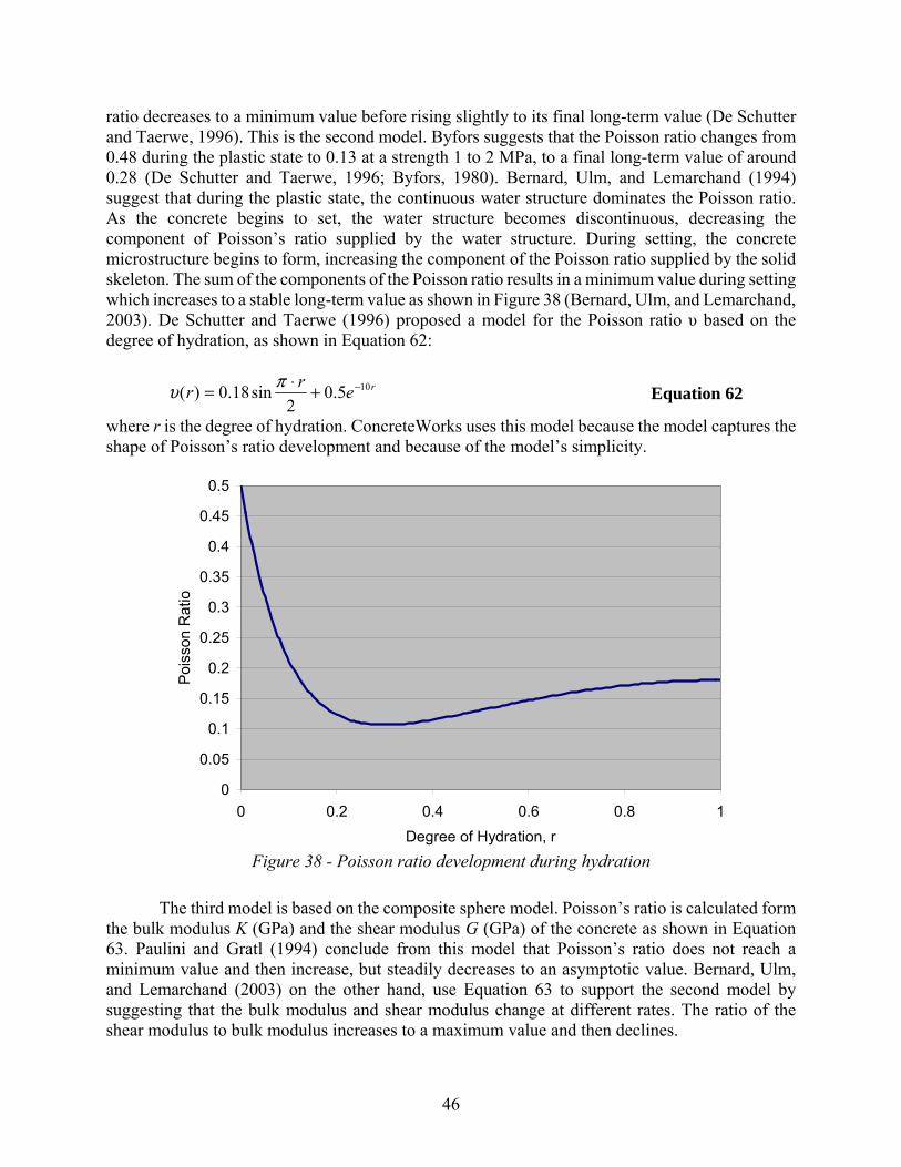
46

ratio decreases to a minimum value before rising slightly to its final long-term value (De Schutter and Taerwe, 1996). This is the second model. Byfors suggests that the Poisson ratio changes from 0.48 during the plastic state to 0.13 at a strength 1 to 2 MPa, to a final long-term value of around 0.28 (De Schutter and Taerwe, 1996; Byfors, 1980). Bernard, Ulm, and Lemarchand (1994) suggest that during the plastic state, the continuous water structure dominates the Poisson ratio. As the concrete begins to set, the water structure becomes discontinuous, decreasing the component of Poisson’s ratio supplied by the water structure. During setting, the concrete microstructure begins to form, increasing the component of the Poisson ratio supplied by the solid skeleton. The sum of the components of the Poisson ratio results in a minimum value during setting which increases to a stable long-term value as shown in Figure 38 (Bernard, Ulm, and Lemarchand, 2003). De Schutter and Taerwe (1996) proposed a model for the Poisson ratio υ based on the degree of hydration, as shown in Equation 62:

rer

r 105.02

sin18.0)( −+⋅= πυ Equation 62

where r is the degree of hydration. ConcreteWorks uses this model because the model captures the shape of Poisson’s ratio development and because of the model’s simplicity.

Figure 38 - Poisson ratio development during hydration

The third model is based on the composite sphere model. Poisson’s ratio is calculated form the bulk modulus K (GPa) and the shear modulus G (GPa) of the concrete as shown in Equation 63. Paulini and Gratl (1994) conclude from this model that Poisson’s ratio does not reach a minimum value and then increase, but steadily decreases to an asymptotic value. Bernard, Ulm, and Lemarchand (2003) on the other hand, use Equation 63 to support the second model by suggesting that the bulk modulus and shear modulus change at different rates. The ratio of the shear modulus to bulk modulus increases to a maximum value and then declines.

0

0.05

0.1

0.15

0.2

0.25

0.3

0.35

0.4

0.45

0.5

0 0.2 0.4 0.6 0.8 1

Degree of Hydration, r

Poi

sson

Rat

io

47

GK

GK

26

23

+−=υ Equation 63

Poisson’s ratio has been found to be equivalent in tension and compression (Lydon and

Balendran, 1986)—a very important point for use in computer models of thermal stresses. ConcreteWorks assumes that the Poisson’s ratio is equal in compression and tension.

The dynamic Poisson ratio is about 25–40% higher than the static Poisson ratio (Byfors, 1980). The dynamic Poisson ratio is thought to be more representative of the actual elastic behavior of concrete (Mindess, Young, and Darwin, 2003). The static Poisson’s ratio has been found to be principally a function of the percent volume of aggregates in the mixture, while the dynamic Poisson’s ratio has been found to be a function of the age, w/cm, and percent volume of aggregates.

Poisson’s ratio has been shown to be constant up to a stress of 50–60% of the compressive strength. Micro-cracking at higher stress levels can change the Poisson’s ratio. Poisson’s ratio may also be different under biaxial or triaxial states of stress (Anson and Newman, 1966). ConcreteWorks assumes that the Poisson’s ratio is independent of the stress level and the state of stress.

4.3.3. Coefficient of Thermal Expansion

The coefficient of thermal expansion (CTE) of concrete is an indicator of the concrete member length change due to temperature changes in the concrete. It is one of the most important parameters in predicting stress distributions in concrete members. Knowledge of the CTE allows researchers to separate the effects of temperature induced deformations from autogenous shrinkage in laboratory tests. Separate models for thermal and autogenous deformations can then be made, allowing for their superposition in computer based stress models. Several factors can affect the CTE, including mixture proportions, aggregate type, degree of saturation, and age.

The hardened concrete CTE is primarily a function of the CTE of the concrete mixture’s constituent materials (Mitchell, 1953; Emanuel and Hulsey, 1977). Because of the volume of aggregates in concrete mixtures, the hardened concrete CTE is dominated by the CTE of the aggregate. Some common values of the CTE for concrete containing different types of aggregates are shown in Table 8. A change in the cementitious material properties such as fineness, type, and composition will also affect the CTE (Mitchell, 1953).

Table 8 - CTE for concretes made with different aggregates (Bamforth and Price, 1995)

Aggregate Type of Concrete

CTE (m/m/°C) CTE (in/in/°F)

Siliceous River Gravel 12.0 6.7 Granite 10.0 5.6 Limestone 8.0 4.4 Lightweight 7.0 3.9

Materials change volume as the temperature changes because the temperature changes the

attractive forces in molecular and atomic structures, as well as capillary stresses. It has been observed that concrete has a higher CTE when partially saturated than at oven dry or saturated. The CTE reaches a maximum value between 60% and 80% relative humidity (Meyers, 1950; Mitchell, 1953; Emanuel and Hulsey, 1977; Walker, Bloem, and Mullen, 1952). As the water in

48

capillary pores expands with temperature, the surface curvature and hence surface tension and capillary under pressure in the pores decreases. This surface-tension-induced volume change does not occur at oven dry conditions or at saturated conditions because the pore has no air-water meniscus in these states (Bjøntegaard, 1999). When autogenous shrinkage occurs in concrete, the relative humidity will drop in the capillary pores to a limiting value of about 75% (Jensen and Hansen, 2001). The CTE will then rise because of the change in relative humidity (Hedlund, 2000), further increasing the development of thermal stresses.

Some researchers have found different coefficients for thermal expansion and contraction (Byfors, 1980; Emborg, 1989). The difference in measured coefficients may be explained by the changing mechanical properties of concrete during young ages, so that the concrete that is measured during the heat phase is different mechanically than that measured during cooling a short time later (Emborg, 1989). Differences between measured coefficients of thermal expansion and contraction may also be due to non-linear effects from differences in the CTE between the concrete and embedded strain gauges (Yamakawa, Nakauchi, Kita, and Onuma, 1986).

As the concrete hydrates, the CTE will change. The fresh concrete CTE is estimated to be 8–10 times greater than the hardened CTE (Schöppel and Springenschmid, 1994). There is debate about how the CTE changes during hydration. Kada, et. al. (2002) measured a decrease in the CTE for a low w/cm mixture (0.30) during the first few hours after setting. The CTE then increased to a stable long-term value. Mixtures with a w/cm of .35 and .4 both showed the CTE decreasing to assume a stable value at around 10 hours. The drop in the CTE and subsequent rise can be attributed to the reduction of relative humidity in the sample because of self desiccation, which increases the CTE. Other researchers have found that the CTE decreases to an asymptotic long-term value (Byfors, 1980; Glisic, 2000). Hashida and Yamaziki (2002) have developed an equation to relate the time of final set to the CTE, as shown in Equation 64:

bt

tat

fscte +

⋅= ln)( 1α Equation 64

where αcte is the concrete CTE (με/°C), a1 and b are fit parameters (με/°C), t is the time, and tfs is the time of final set. The parameters a1 and b are dependent on the w/cm, supplementary cementitious materials, cement type, and aggregates used.

ConcreteWorks uses a constant CTE, because of the lack of a data to model how the mixture proportions relate to CTE development. Because the CTE decreases very rapidly before the time of set, little loss in accuracy is expected from using a constant value except in the case of low w/cm where the CTE may increase after set and during curing. The constant CTE used in ConcreteWorks is calculated from the mixture proportions and the aggregate type using the method proposed by Emanual and Hulsey (1977) shown in Equation 65.

pfaca

ppfafacacacteh VVV

VVV

++⋅+⋅+⋅

=ααα

α Equation 65

where αcteh is the hardened concrete CTE, αca is the coarse aggregate CTE (με/°C), Vca is the coarse aggregate volume (kg/m3), αfa is the fine aggregate CTE (με/°C), Vfa is the fine aggregate volume (kg/m3), αp is the paste CTE (με/°C), and Vp is the paste volume (kg/m3). In order to simplify the inputs, ConcreteWorks uses the assumed material specific gravity values for constituent materials shown in Table 9 in calculating the hardened concrete CTE. The assumed constituent material CTE values are shown in Table 10. Material CTE and specific gravity values can vary

49

substantially, and may affect the calculated CTE value substantially. The values selected for use in ConcreteWorks were selected to represent typical, commonly used Texas materials. For more accurate results, it is suggested that the user test and input into ConcreteWorks the hardened concrete CTE of the specific materials used.

Table 9 - Concrete constituent materials assumed specific gravity values

Material Specific Gravity Water 1

Cement 3.14 Class F Fly

Ash 2.4 Class C Fly

Ash 2.7 Slag 2.87

UFFA 2.57 Silica Fume 2.2

Coarse Aggregate 2.65

Fine Aggregate 2.65

Table 10 - Concrete constituent materials assumed CTE

Material CTE values used in

ConcreteWorks (με/°C) CTE from Emanuel and Hulsey,

1977 (με/°C) Hardened Cement Paste 10.8 10.8 Limestone Aggregate 3.5 3.5–6 Siliceous River Gravel

and Sand 11 11–12.5

Granite Aggregate 7.5 6.5–8.5 Dolomitic Limestone

Aggregate 7 7–10

4.3.4. Autogenous Shrinkage Model

The volume of the cement hydration products is less than the volume of the cement before hydration. In low w/cm concrete, all of the water will be used to react with the cement. The unhydrated cement will then react with the water in the concrete pores, drying the pores and causing shrinkage. ConcreteWorks uses a modified version of the autogenous shrinkage model developed by Hedlund (2000). Hedlund developed a model based on his testing and that found in the literature for autogenous shrinkage starting at 24 equivalent age hours. The model is based on an ultimate autogenous shrinkage calculated from the w/cm which is altered to account for temperature effects. Equation 66-69 show the equations proposed by Hedlund for calculating the autogenous shrinkage with the concrete equivalent age:

)()(0 Tt STessuSH ββεε ⋅⋅= Equation 66

50

310)3.165.0( −⋅⋅+−=cm

wsuε Equation 67

−

−=SH

s

ses tt

tt

η

β0

10 exp)( Equation 68

−−⋅+

−−⋅+=

21

22

110 exp1exp1)(

bb

ST T

Ta

T

TaaTβ Equation 69

where ts0 (days), ts1 (days), ηSH, a0, a1, a2, b1, b2, T1 (°C), and T2 (°C) are fit parameters. Hedlund recommends setting the parameters ts1, ηSH, a0, a1, b1, b2, T1 (°C), and T2 (°C) may be set equal to 5 days, 0.3, 0.4, 0.6, 9 °C, 2.9, 55 °C, and 7, respectively. Additionally, he recommends setting the parameter a2 may be set equal to 1.3 for normal strength concrete and 0.1 for high performance concrete. The parameter ts0 is the time at which the concrete shrinkage begins. Before this time, the concrete autogenous shrinkage is set equal to zero (Hedlund, 2000).

The autogenous shrinkage model used in ConcreteWorks modifies the model developed by Hedlund to reduce the w/cm at which autogenous shrinkage develops, the time at which autogenous shrinkage begins, and does not include the temperature modification term. The ultimate concrete shrinkage value used in ConcreteWorks is calculated using Equation 70:

( ) 310/238.294.0 −⋅⋅+−= cmwaultε Equation 70

The w/cm ratio at which autogenous shrinkage develops in ConcreteWorks is 0.42, which corresponds to the theoretical w/cm at which complete hydration is possible (Mindess, Young, and Darwin, 2003). Additionally, autogenous shrinkage begins at the virtual time of set, not at 24 equivalent age hours as in the Hedlund model. The autogenous shrinkage model will be improved in future versions of ConcreteWorks as more data and models become available.

4.4. Elastic Stress and Degree of Restraint

The restraint is needed at each point in the concrete member at each time step to be able to accurately model the stresses in the concrete. The restraint can be obtained by performing a structural analysis of the concrete member with non-uniform material properties across the cross section. ConcreteWorks uses a plane strain finite-difference scheme to calculate the elastic stress in the member. The software considers the non-homogenous material development of the member by assuming a constant modulus and Poisson ratio for each control volume. The elastic modulus and Poisson ratio for each control volume is different, and is based on the maturity for the case of the elastic modulus and the degree of hydration for the Poisson ratio. The restraint case modeled for the rectangular column is the same as that shown in Figure 4, a two-dimensional horizontal cross section of the column. The restraint case modeled for the rectangular bent cap is the same as that shown in Figure 14, a two-dimensional vertical cross section of the cap. Footings are modeled assuming a two-dimensional cross section as shown in Figure 7, assuming a fixed base condition. The state of stress in the rectangular column and bent cap can be adequately represented using the two-dimensional models assumed because the stress in the third direction should be relatively small compared to the other two dimensions. The footing model, however, may deviate from the actual member stresses because the stress in the third dimension may not be small relative to the

51

other two dimensions. Care should be taken in interpreting results from the footing model in ConcreteWorks. Improvements in the footing elastic stress calculation module are being considered for future versions of ConcreteWorks.

After the elastic stress is calculated, the elastic strain is then calculated using Hooke’s law, as shown in Equation 71–73.

[ ]E

yxx

συσε

⋅−=

Equation 71

[ ]E

xyy

συσε

⋅−= Equation 72

( )E

xyxy

υσε

+⋅⋅=

12 Equation 73

where εx is the strain in the x direction, σx is the stress in the x direction (MPa), ν is the Poisson ratio, σy is the stress in the y direction (MPa), εy is the strain in the y direction, εxy is the shear strain in the xy direction, σxy is the shear stress in the xy direction, and E is the elastic modulus (MPa).

4.5. Early-Age Concrete Creep Model

Creep may be defined as a time-dependent deformation during a constant stress. Stress relaxation may be defined as a time dependent decrease in stress during a constant strain. Creep is applied to the stresses in the x, y and xy directions independently. The uniaxial constitutive equation for concrete creep is shown in Equation 74.

+⋅=t

ttdttJt0

000 )()(),()( εσε Equation 74

where ε is the total strain, t is the time, t0 is the time of the load application, J(t,t0) is the creep compliance, dσ(t0) is the stress imposed at time t0, and ε0 is the instantaneous or elastic response to the stress application.

Creep is applied to the elastic strains using the principle of superposition. The principle of superposition assumes that a step stress function is applied, with a corresponding strain response. The strain responses are then superimposed using the assumption of linearity as shown in Figure 39. The assumption of linearity is probably a valid assumption up to stress levels of about 40% (Emborg, 1998b). The two obvious problems with the approach used in ConcreteWorks are 1) the thermal stresses calculated in the model can exceed 40% of the tensile strength and 2) the model assumes linearity. The second assumption is a simplification necessary for simplicity and to reduce the runtime of the analysis. This assumption is definitely not true. Because the stresses in the member are relieved non-linearly by stress relaxation, the thermal stresses would redistribute in the member. These assumptions, however, do not preclude ConcreteWorks from being used in design. High tensile stresses should be avoided during the design stage to prevent damage from micro-cracking and potential through cracks.

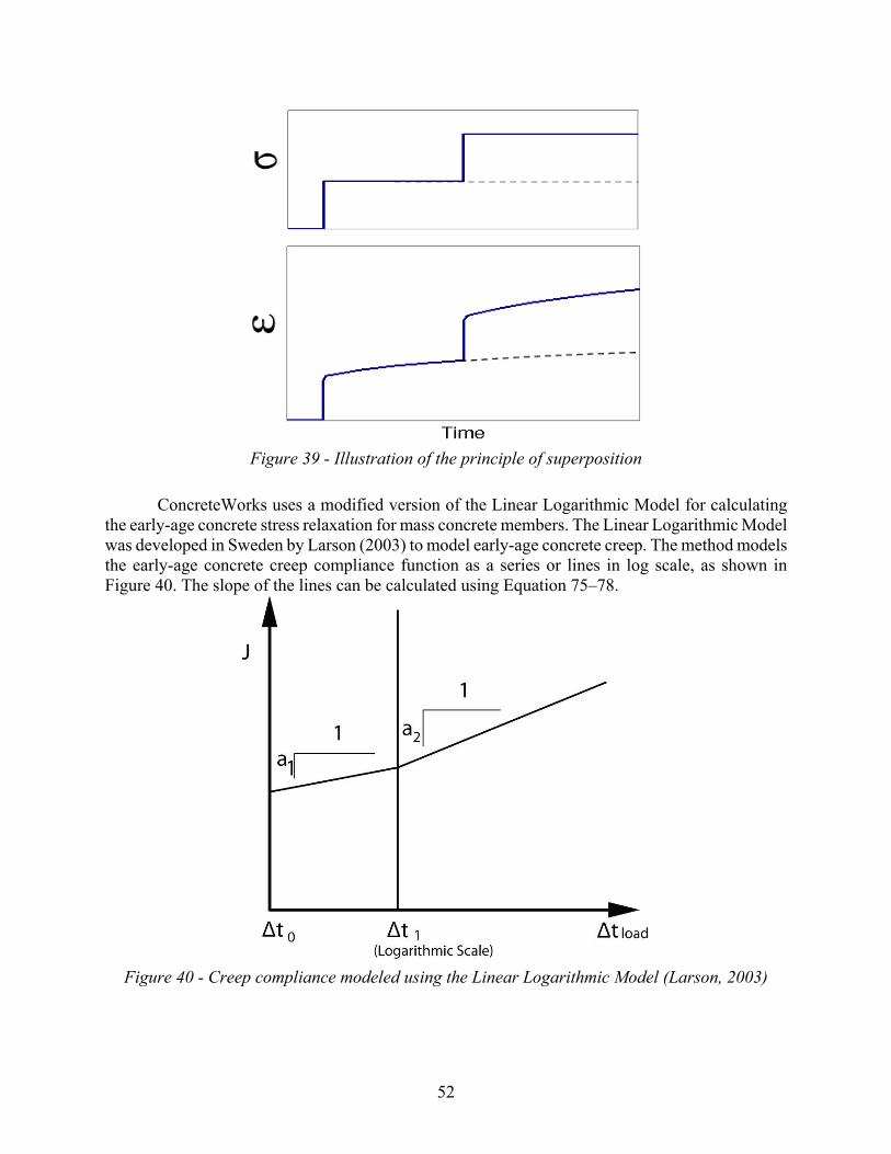
52

Figure 39 - Illustration of the principle of superposition

ConcreteWorks uses a modified version of the Linear Logarithmic Model for calculating the early-age concrete stress relaxation for mass concrete members. The Linear Logarithmic Model was developed in Sweden by Larson (2003) to model early-age concrete creep. The method models the early-age concrete creep compliance function as a series or lines in log scale, as shown in Figure 40. The slope of the lines can be calculated using Equation 75–78.

Figure 40 - Creep compliance modeled using the Linear Logarithmic Model (Larson, 2003)

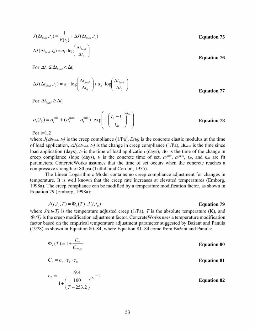
53

),()(

1),( 0

00 ttJ

tEttJ loadload ΔΔ+=Δ Equation 75

Δ

Δ⋅=ΔΔ0

10 log),(t

tattJ load

load

For 10 ttt load Δ<Δ≤Δ

Equation 76

Δ

Δ⋅+

Δ

Δ⋅=ΔΔ0

20

10 loglog),(t

ta

t

tattJ loadload

load

For 1ttload Δ≥Δ

Equation 77

−−⋅−+=ain

ai

siiii t

ttaaata 0minmaxmin

0 exp)()(

For i=1,2

Equation 78

where J(Δtload, t0) is the creep compliance (1/Pa), E(t0) is the concrete elastic modulus at the time of load application, ΔJ(Δtload, t0) is the change in creep compliance (1/Pa), Δtload is the time since load application (days), t0 is the time of load application (days), Δt1 is the time of the change in creep compliance slope (days), ts is the concrete time of set, ai

min, aimax, tai, and nai are fit

parameters. ConcreteWorks assumes that the time of set occurs when the concrete reaches a compressive strength of 80 psi (Tuthill and Cordon, 1955). The Linear Logarithmic Model contains no creep compliance adjustment for changes in temperature. It is well known that the creep rate increases at elevated temperatures (Emborg, 1998a). The creep compliance can be modified by a temperature modification factor, as shown in Equation 79 (Emborg, 1998a):

),()(),,( 00 ttJTTttJ c ⋅Φ= Equation 79where J(t,t0,T) is the temperature adjusted creep (1/Pa), T is the absolute temperature (K), and Φc(T) is the creep modification adjustment factor. ConcreteWorks uses a temperature modification factor based on the empirical temperature adjustment parameter suggested by Bažant and Panula (1978) as shown in Equation 80–84, where Equation 81–84 come from Bažant and Panula:

TMF

Tc C

CT +=Φ 1)( Equation 80

0ccC TTT ⋅⋅= τ Equation 81

1

2.253

1001

4.195.3

−

−+

=

T

cT Equation 82

54

78.0

)(

601

1

69.0

+

+

=

T

T

t

τ Equation 83

1

2

0 8

1a

cm

a

cm

wc ⋅

⋅

⋅

= Equation 84

where CTMF is a fit parameter equal to 2.5, tT is the concrete age at the time the temperature is applied, w is the water content (kg/m3), cm is the cementing materials content (kg/m3), a is the aggregate content (kg/m3), a1 is a constant that accounts for the type of cement used.

4.5.1. LLM Creep Parameter Estimates

The creep parameters used in ConcreteWorks for the LLM model are based on a statistical model developed from early-age rigid cracking frame tests on 36 different concrete mixtures. A few of these mixtures were tested under several different temperature histories, in order to quantify the effects of temperature on concrete early-age creep. The creep parameters ta1, ta2, and na2 are calculated from the concrete mixture proportions and constituent material properties according to Equation 85-87 when the Rietveld method (Rietveld, 1969) of determining the cement composition is used (Riding, 2007):

FerritecmwFAta ⋅−⋅+⋅+= 00965.0)/ln(429.00064.0680.01 Equation 85

)0556.0

)(10078.0

/7169.3)(0192.0671.3exp(2

Ferrite

ArcaniteAnhydriteeHemihydratGypsum

cmwGGBFSFAta

⋅−+++⋅

−⋅−+⋅−=

Equation 86

)/194.5253.0177.0)ln(586.6

072.00705.0735.26exp(2

cmwAlumFerriteAlite

GGBFSFAna

⋅+⋅−⋅−⋅+⋅+⋅+−=

Equation 87

where FA is the percent fly ash replacement of cement by mass, w/cm is the water-to-cementing-materials ratio, Ferrite is the percent ferrite of the cement, as determined by Rietveld analysis, GGBFS is the percent grade 120 ground granulated blast furnace slag replacement of cement by mass, Gypsum is the percent gypsum of the cement, as determined by Rietveld analysis, Hemihydrate is the percent hemihydrate in the cement, as determined by Rietveld analysis, Anhydrite is the percent anhydrite in the cement, as determined by Rietveld analysis, Alite is the percent alite in the cement, as determined by Rietveld analysis, and Alum in the percent aluminate in the cement as determined by Rietveld analysis. When a supplementary cementing material is used, the percent values used of the cement chemistry are the percent of the material in the cement times the percent cement of the total cementing materials.

When the Bogue method (ASTM C 150) of determining the cement composition is used, Equation 88-90 are used to relate the mixture proportions and constituent material properties to the early age MLLM creep parameters ta1, ta2, na2 (Riding, 2007):

AFCwcmFAta 41 0111.0)ln(448.00061.0728.0 ⋅−⋅+⋅+= Equation 88

55

)0566.00186.0

404.3)(0179.0436.3exp(

42

2

AFCSC

wcmGGBFSFAta

⋅−⋅−⋅−+⋅−=

Equation 89

)0107.0572.0425.0

00869.00619.00541.0165.6exp(

43

2

CemBlaineAFCAC

cementGGBFSFAna

⋅+⋅−⋅−⋅−⋅−⋅−=

Equation 90

where C4AF is the percent C4AF of the cement, as calculated using the Bogue method, C2S is the percent C2S of the cement, as calculated using the Bogue method, C3A is the percent C3A of the cement, as calculated using the Bogue method, cement is the total amount of cementing materials used in lb/yd3, and CemBlaine is the cement Blaine fineness (m2/kg). When a supplementary cementing material is used, the percent values used of the cement chemistry are the percent of the material in the cement times the percent cement of the total cementing materials. The remainders of the MLLM creep parameters are kept constant, according to Table 11:

Table 11 - Modified linear logarithmic model parameters assumed to remain constant in ConcreteWorks

Modified Linear Logarithmic Model Parameter

Value Units

Δt0 0.001 days Δt1 0.1 days a1

min (*10^-12) 0.1 1/Pa a1

max (*10^-12) 60 1/Pa na1 1.19 a2

min (*10^-12) 5 1/Pa a2

max (*10^-12) 30 1/Pa

4.6. Cracking Potential

In ConcreteWorks, the cracking potential classification of a mass concrete member is based on the calculated tensile stress-to-tensile strength ratio. The concrete tensile-stress-to-tensile-strength ratio calculated in the software is assigned a cracking probability classification using the probability density shown in Figure 41. The cracking probability density was obtained from the distribution of the tensile stress-to-splitting tensile strength at cracking in the rigid cracking frame tests performed.

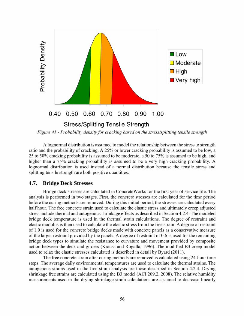
56

Figure 41 - Probability density for cracking based on the stress/splitting tensile strength

A lognormal distribution is assumed to model the relationship between the stress to strength ratio and the probability of cracking. A 25% or lower cracking probability is assumed to be low, a 25 to 50% cracking probability is assumed to be moderate, a 50 to 75% is assumed to be high, and higher than a 75% cracking probability is assumed to be a very high cracking probability. A lognormal distribution is used instead of a normal distribution because the tensile stress and splitting tensile strength are both positive quantities.

4.7. Bridge Deck Stresses

Bridge deck stresses are calculated in ConcreteWorks for the first year of service life. The analysis is performed in two stages. First, the concrete stresses are calculated for the time period before the curing methods are removed. During this initial period, the stresses are calculated every half hour. The free concrete strain used to calculate the elastic stress and ultimately creep adjusted stress include thermal and autogenous shrinkage effects as described in Section 4.2.4. The modeled bridge deck temperature is used in the thermal strain calculations. The degree of restraint and elastic modulus is then used to calculate the elastic stress from the free strain. A degree of restraint of 1.0 is used for the concrete bridge decks made with concrete panels as a conservative measure of the larger restraint provided by the panels. A degree of restraint of 0.6 is used for the remaining bridge deck types to simulate the resistance to curvature and movement provided by composite action between the deck and girders (Krauss and Rogalla, 1996). The modified B3 creep model used to relax the elastic stresses calculated is described in detail by Byard (2011). The free concrete strain after curing methods are removed is calculated using 24-hour time steps. The average daily environmental temperatures are used to calculate the thermal strains. The autogenous strains used in the free strain analysis are those described in Section 4.2.4. Drying shrinkage free strains are calculated using the B3 model (ACI 209.2, 2008). The relative humidity measurements used in the drying shrinkage strain calculations are assumed to decrease linearly

0.40 0.50 0.60 0.70 0.80 0.90 1.00

Stress/Splitting Tensile Strength

Pro

ba

bili

ty D

en

sity

Low

Moderate

High

Very high

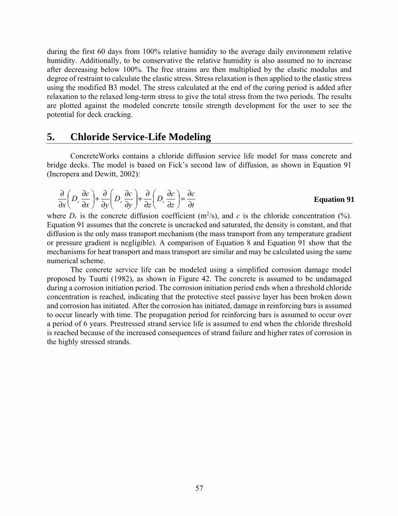
57

during the first 60 days from 100% relative humidity to the average daily environment relative humidity. Additionally, to be conservative the relative humidity is also assumed no to increase after decreasing below 100%. The free strains are then multiplied by the elastic modulus and degree of restraint to calculate the elastic stress. Stress relaxation is then applied to the elastic stress using the modified B3 model. The stress calculated at the end of the curing period is added after relaxation to the relaxed long-term stress to give the total stress from the two periods. The results are plotted against the modeled concrete tensile strength development for the user to see the potential for deck cracking.

5. Chloride Service-Life Modeling

ConcreteWorks contains a chloride diffusion service life model for mass concrete and bridge decks. The model is based on Fick’s second law of diffusion, as shown in Equation 91 (Incropera and Dewitt, 2002):

t

c

z

cD

zy

cD

yx

cD

x ccc ∂∂=

∂∂

∂∂+

∂∂

∂∂+

∂∂

∂∂

Equation 91

where Dc is the concrete diffusion coefficient (m2/s), and c is the chloride concentration (%). Equation 91 assumes that the concrete is uncracked and saturated, the density is constant, and that diffusion is the only mass transport mechanism (the mass transport from any temperature gradient or pressure gradient is negligible). A comparison of Equation 8 and Equation 91 show that the mechanisms for heat transport and mass transport are similar and may be calculated using the same numerical scheme. The concrete service life can be modeled using a simplified corrosion damage model proposed by Tuutti (1982), as shown in Figure 42. The concrete is assumed to be undamaged during a corrosion initiation period. The corrosion initiation period ends when a threshold chloride concentration is reached, indicating that the protective steel passive layer has been broken down and corrosion has initiated. After the corrosion has initiated, damage in reinforcing bars is assumed to occur linearly with time. The propagation period for reinforcing bars is assumed to occur over a period of 6 years. Prestressed strand service life is assumed to end when the chloride threshold is reached because of the increased consequences of strand failure and higher rates of corrosion in the highly stressed strands.

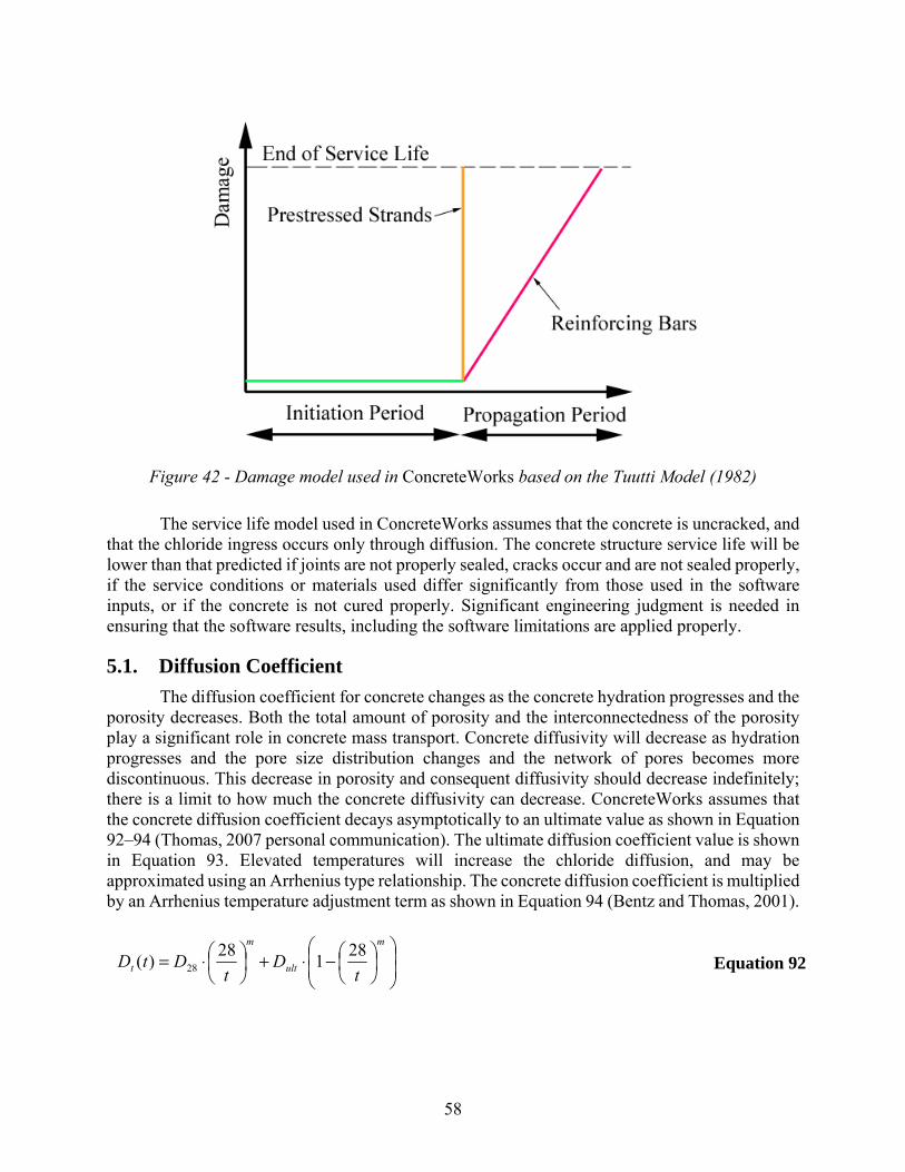
58

Figure 42 - Damage model used in ConcreteWorks based on the Tuutti Model (1982)

The service life model used in ConcreteWorks assumes that the concrete is uncracked, and that the chloride ingress occurs only through diffusion. The concrete structure service life will be lower than that predicted if joints are not properly sealed, cracks occur and are not sealed properly, if the service conditions or materials used differ significantly from those used in the software inputs, or if the concrete is not cured properly. Significant engineering judgment is needed in ensuring that the software results, including the software limitations are applied properly.

5.1. Diffusion Coefficient

The diffusion coefficient for concrete changes as the concrete hydration progresses and the porosity decreases. Both the total amount of porosity and the interconnectedness of the porosity play a significant role in concrete mass transport. Concrete diffusivity will decrease as hydration progresses and the pore size distribution changes and the network of pores becomes more discontinuous. This decrease in porosity and consequent diffusivity should decrease indefinitely; there is a limit to how much the concrete diffusivity can decrease. ConcreteWorks assumes that the concrete diffusion coefficient decays asymptotically to an ultimate value as shown in Equation 92–94 (Thomas, 2007 personal communication). The ultimate diffusion coefficient value is shown in Equation 93. Elevated temperatures will increase the chloride diffusion, and may be approximated using an Arrhenius type relationship. The concrete diffusion coefficient is multiplied by an Arrhenius temperature adjustment term as shown in Equation 94 (Bentz and Thomas, 2001).

−⋅+

⋅=

m

ult

m

t tD

tDtD

281

28)( 28 Equation 92

59

m

ult DD

⋅=

36500

2828 Equation 93

−⋅⋅=

TTR

UtDTtD

refttT

11exp)(),( Equation 94

where Dt(t) is the concrete diffusion coefficient (m2/s) at time t (days), D28 is the 28-day concrete diffusion coefficient (m2/s), m is the concrete diffusion decay constant, U is the diffusion process activation energy, which can be assumed to 35000 J/mol, R is the universal gas constant (8.314 J/K/mol), Tref is the concrete diffusion coefficient reference temperature (293 K), and T is the temperature of the concrete (K). Figure 43 and Figure 44 show the effect of a change in the 28-day concrete diffusion coefficient D28 and the decay constant m on the concrete apparent diffusion coefficient.

Figure 43 - Effect of a change in the decay constant m on the concrete apparent diffusion

coefficient Dt

1.0E-14

1.0E-13

1.0E-12

1.0E-11

10 100 1000 10000 100000 1000000Age, t (days)

Dt

(m2/s

)

m = 0.26m = 0.46m = 0.66

D28=8x10-12

60

Figure 44 - Effect of a change in the 28-day apparent diffusion coefficient on the concrete

apparent diffusion coefficient Dt with time

ConcreteWorks uses the yearly temperature profile calculated from the weather data files for the city selected in Equation 94. The value for each temperature point used in the yearly temperature profile is calculated as the average of the 24 hourly temperature points for the day selected. When the user selects 12 temperature points per year, the 12 temperature data points are calculated using the first day of each month. When the user selects 24 points per year, the 24 temperature data points are calculated using the first and fifteenth days of each month. When the user selects 52 temperature points per year, a temperature point is calculated for every 7 days.

All concrete bulk diffusion material models used in ConcreteWorks were developed by Mike Thomas at the University of New Brunswick (UNB) based on tests performed according to ASTM C 1556. The literature reports many differences in reported chloride diffusion values because of differences in material, testing conditions, and analysis method. Because the materials used were well characterized, the testing and analysis methods are known, and for consistency, only data collected at the University of Toronto (UT) and UNB was used in developing the concrete diffusion coefficient material models used in ConcreteWorks (Mike Thomas, 2007 Personal Communication).

5.2. Water-to-Cementitious-Materials Ratio

The water-to-cementitious-materials ratio (w/cm) is a major factor in the chloride diffusion coefficient. It is well known that the concrete porosity and consequently permeability decreases as the w/cm decreases (Mindess, Young, and Darwin, 2003). The base 28-day diffusion coefficient D28 used in ConcreteWorks is calculated using the w/cm as shown in Equation 95:

1.0E-13

1.0E-12

1.0E-11

10 100 1000 10000 100000 1000000Age, t (days)

Dt

(m2/s

)

D = 8x10D = 4x10D = 1x10

m=0.26-12

-12

-12

61

279.0

/12

28 1017.2cmw

eD ⋅⋅= − Equation 95

Figure 45 shows the test results from a study performed at UNB and UT used to model the effect of w/cm ratio on the concrete 28-day bulk diffusion value. All of the tests shown in Figure 45 were cast with a type I cement with 12% C3A, with w/cm ratio varying between 0.2 and 0.8, and cement contents varying between 225 and 725 kg/m3 (Mike Thomas, 2007 Personal Communication).

Figure 45 - Relationship between 28-day concrete apparent diffusion coefficient and w/cm

5.2.1. Supplementary Cementing Materials

Supplementary cementing materials can reduce the diffusivity of concrete by reducing the porosity and pore size distribution of concrete (Mindess, Young, and Darwin, 2003). Ultra-fine fly ash and silica fume will reduce the 28-day diffusivity by particle packing and the pozzolanic reaction that will occur at a faster rate because of the high surface area. The effect of ultra-fine fly ash and silica fume on concrete 28-day diffusivity is calculated in ConcreteWorks using Equation 96 and Equation 97:

( )07.6/829.0170.0 UFFA

PC

UFFA eD

D −+= Equation 96

( )51.2/794.0206.0 SF

PC

SF eD

D −+= Equation 97

where DUFFA is 28-day diffusivity of concrete containing ultra-fine fly ash (m2/s), DPC is the 28-day diffusivity of concrete containing no supplementary cementing materials (m2/s), UFFA is the percent replacement of cement with ultra-fine fly ash, DSF is the 28-day diffusivity of concrete containing silica fume (m2/s), and SF is the percent replacement of cement with silica fume. The concrete diffusivity adjustments used for silica fume replacement are based on bulk concrete

1.0E-12

1.0E-11

1.0E-10

0.2 0.4 0.6 0.8W/CM

28

-da

y D

iffu

sio

n C

oe

ffici

en

t, D28

(m

2 /s)

UNB (UT Study)

Best-fit exponential

R2 = 0.931 ( ) 195.0//131228 1040.51087.1 −−−− ×+×= CMWeD

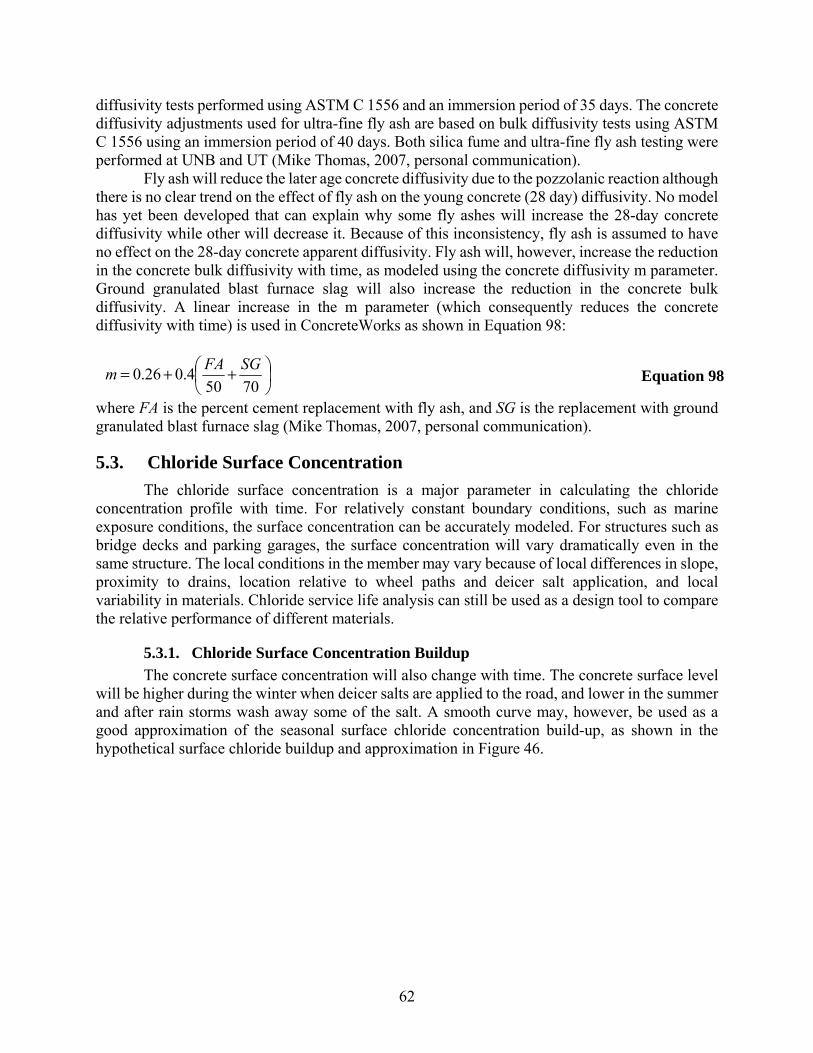
62

diffusivity tests performed using ASTM C 1556 and an immersion period of 35 days. The concrete diffusivity adjustments used for ultra-fine fly ash are based on bulk diffusivity tests using ASTM C 1556 using an immersion period of 40 days. Both silica fume and ultra-fine fly ash testing were performed at UNB and UT (Mike Thomas, 2007, personal communication).

Fly ash will reduce the later age concrete diffusivity due to the pozzolanic reaction although there is no clear trend on the effect of fly ash on the young concrete (28 day) diffusivity. No model has yet been developed that can explain why some fly ashes will increase the 28-day concrete diffusivity while other will decrease it. Because of this inconsistency, fly ash is assumed to have no effect on the 28-day concrete apparent diffusivity. Fly ash will, however, increase the reduction in the concrete bulk diffusivity with time, as modeled using the concrete diffusivity m parameter. Ground granulated blast furnace slag will also increase the reduction in the concrete bulk diffusivity. A linear increase in the m parameter (which consequently reduces the concrete diffusivity with time) is used in ConcreteWorks as shown in Equation 98:

++=

70504.026.0

SGFAm Equation 98

where FA is the percent cement replacement with fly ash, and SG is the replacement with ground granulated blast furnace slag (Mike Thomas, 2007, personal communication).

5.3. Chloride Surface Concentration

The chloride surface concentration is a major parameter in calculating the chloride concentration profile with time. For relatively constant boundary conditions, such as marine exposure conditions, the surface concentration can be accurately modeled. For structures such as bridge decks and parking garages, the surface concentration will vary dramatically even in the same structure. The local conditions in the member may vary because of local differences in slope, proximity to drains, location relative to wheel paths and deicer salt application, and local variability in materials. Chloride service life analysis can still be used as a design tool to compare the relative performance of different materials.

5.3.1. Chloride Surface Concentration Buildup

The concrete surface concentration will also change with time. The concrete surface level will be higher during the winter when deicer salts are applied to the road, and lower in the summer and after rain storms wash away some of the salt. A smooth curve may, however, be used as a good approximation of the seasonal surface chloride concentration build-up, as shown in the hypothetical surface chloride buildup and approximation in Figure 46.

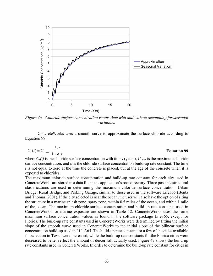
63

Figure 46 - Chloride surface concentration versus time with and without accounting for seasonal

variations

ConcreteWorks uses a smooth curve to approximate the surface chloride according to Equation 99:

tb

tbCtC ss ⋅+

⋅⋅=1

)( max Equation 99

where Cs(t) is the chloride surface concentration with time t (years), Csmax is the maximum chloride surface concentration, and b is the chloride surface concentration build-up rate constant. The time t is not equal to zero at the time the concrete is placed, but at the age of the concrete when it is exposed to chlorides. The maximum chloride surface concentration and build-up rate constant for each city used in ConcreteWorks are stored in a data file in the application’s root directory. Three possible structural classifications are used in determining the maximum chloride surface concentration: Urban Bridge, Rural Bridge, and Parking Garage, similar to those used in the software Life365 (Bentz and Thomas, 2001). If the city selected is near the ocean, the user will also have the option of siting the structure in a marine splash zone, spray zone, within 0.5 miles of the ocean, and within 1 mile of the ocean. The maximum chloride surface concentration and build-up rate constants used in ConcreteWorks for marine exposure are shown in Table 12. ConcreteWorks uses the same maximum surface concentration values as found in the software package Life365, except for Florida. The build-up rate constants used in ConcreteWorks were determined by fitting the initial slope of the smooth curve used in ConcreteWorks to the initial slope of the bilinear surface concentration build-up used in Life-365. The build-up rate constant for a few of the cities available for selection in Texas were increased, while the build-up rate constants for the Florida cities were decreased to better reflect the amount of deicer salt actually used. Figure 47 shows the build-up rate constants used in ConcreteWorks. In order to determine the build-up rate constant for cities in

0

1

2

3

4

5

6

7

8

9

10

0 5 10 15 20

Time (Yrs)

Ch

lorid

e C

once

ntra

tion

(kg

/m3 )

ApproximationSeasonal Variation

64

ConcreteWorks that were not available in Life365, the annual snowfall for each city was compared to that of other cities in the same state for which values were available in Life365. This approach is expected to give a reasonable approximation for these cities, because states usually have uniform deicer salting policies. The maximum surface concentrations used for different exposure conditions corresponding to the build-up rate constant are shown in Table 13.

Table 12 - Chloride surface concentration constants used in ConcreteWorks for marine exposure

Exposure condition Maximum surface concentration (%)

Build-up rate constant

Splash zone 0.8 Instantaneous Spray zone 1 0.15 Within 0.5 miles of ocean

0.6 0.06

Within 1 mile of ocean 0.6 0.03

Figure 47 - Build-up rate constants used in ConcreteWorks

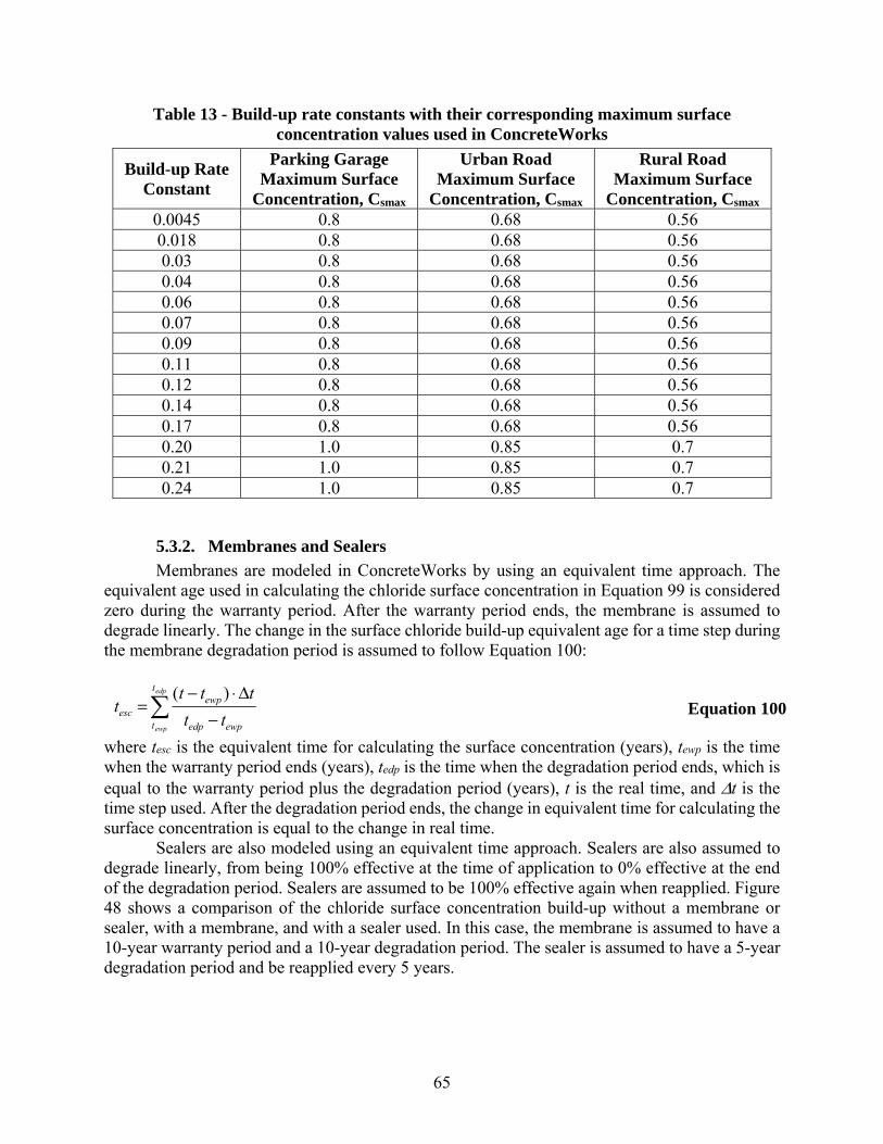
65

Table 13 - Build-up rate constants with their corresponding maximum surface concentration values used in ConcreteWorks

Build-up Rate Constant

Parking Garage Maximum Surface

Concentration, Csmax

Urban Road Maximum Surface

Concentration, Csmax

Rural Road Maximum Surface

Concentration, Csmax

0.0045 0.8 0.68 0.56 0.018 0.8 0.68 0.56 0.03 0.8 0.68 0.56 0.04 0.8 0.68 0.56 0.06 0.8 0.68 0.56 0.07 0.8 0.68 0.56 0.09 0.8 0.68 0.56 0.11 0.8 0.68 0.56 0.12 0.8 0.68 0.56 0.14 0.8 0.68 0.56 0.17 0.8 0.68 0.56 0.20 1.0 0.85 0.7 0.21 1.0 0.85 0.7 0.24 1.0 0.85 0.7

5.3.2. Membranes and Sealers

Membranes are modeled in ConcreteWorks by using an equivalent time approach. The equivalent age used in calculating the chloride surface concentration in Equation 99 is considered zero during the warranty period. After the warranty period ends, the membrane is assumed to degrade linearly. The change in the surface chloride build-up equivalent age for a time step during the membrane degradation period is assumed to follow Equation 100:

−Δ⋅−

=edp

ewp

t

t ewpedp

ewpesc tt

tttt

)( Equation 100

where tesc is the equivalent time for calculating the surface concentration (years), tewp is the time when the warranty period ends (years), tedp is the time when the degradation period ends, which is equal to the warranty period plus the degradation period (years), t is the real time, and Δt is the time step used. After the degradation period ends, the change in equivalent time for calculating the surface concentration is equal to the change in real time.

Sealers are also modeled using an equivalent time approach. Sealers are also assumed to degrade linearly, from being 100% effective at the time of application to 0% effective at the end of the degradation period. Sealers are assumed to be 100% effective again when reapplied. Figure 48 shows a comparison of the chloride surface concentration build-up without a membrane or sealer, with a membrane, and with a sealer used. In this case, the membrane is assumed to have a 10-year warranty period and a 10-year degradation period. The sealer is assumed to have a 5-year degradation period and be reapplied every 5 years.

66

Figure 48 - Chloride surface concentration for cases where no barrier protection method is

used, a membrane is used, and a sealer is used

5.4. Chloride Threshold

In ConcreteWorks, corrosion is assumed to initiate after the chloride concentration at the steel reaches a threshold value. A one-size fits all corrosion threshold value is certainly not valid. Many different chloride threshold values are published in literature. However, a comprehensive model for determining the chloride threshold value from the temperature, relative humidity, mixture proportions, and steel type used does not currently exist. A single chloride threshold value that is dependent on the type of steel chosen is a reasonable assumption for design. A chloride threshold value of 0.07% chloride by mass of concrete is used for black steel and epoxy coated steel (need references). A chloride threshold value of 0.7% chloride by mass of concrete is used for grade 316 Stainless steel.

ConcreteWorks contains inputs for two types of corrosion inhibitors, calcium-nitrite-based corrosion inhibitors or amines and esters. ConcreteWorks uses the same chloride threshold values as Life365 when a corrosion inhibitor is used, as shown in Table 14. Corrosion inhibitors in ConcreteWorks are only used in the cast-in-place concrete. This means that if the user selects a precast panel to be used with a bridge deck, the chloride threshold value of the steel in the precast panel does not change when a corrosion inhibitor is used in cast-in-place concrete above it. In addition, like Life365, the diffusion coefficient is reduced by 10% and the chloride surface concentration build-up rate constant is also reduced by 50% when amines and esters are selected.

0

1

2

3

4

5

6

7

8

9

10

0 10 20 30 40 50 60

Time (Yrs)

Chl

orid

e C

once

ntra

tion

(kg/

m3 )

no protectionmembranesealer

67

Table 14 - Chloride threshold values assumed for black steel based on corrosion inhibitor dose

Corrosion Inhibitor and Dosage Chloride Threshold Value (% of Concrete) Calcium Nitrite at 10 L/m3 0.15 Calcium Nitrite at 15 L/m3 0.24 Calcium Nitrite at 20 L/m3 0.32 Calcium Nitrite at 25 L/m3 0.37 Calcium Nitrite at 30 L/m3 0.40 Amines and Esters at 5 L/m3 0.12

5.5. Initial Chloride Profile

ConcreteWorks contains an option to model the chloride diffusion considering an initial chloride profile. This initial chloride concentration profile may be used because of the addition of a significant amount of chlorides in the concrete mixture (such as the ill-advised use of sea water instead of fresh water or the use of a calcium-chloride based admixture in reinforced concrete). Additionally, the initial chloride profile may be used to enter the chloride profile obtained from performing chloride profile grinding of the actual structure. Considerable engineering judgment should be used in performing this type of test and the subsequent service life analysis. Chloride profile tests can be highly variable depending on the location in the structure because of local water runoff conditions and local variability in the concrete cover quality. When an existing structure is modeled, the age of the structure is added to the time used in determining the chloride surface concentration and the concrete diffusion coefficients. The default chloride surface concentration constants should be altered to account for the actual concrete chloride surface concentration and the expected future concentrations. This type of analysis should only be performed by those intimately familiar with the service life calculation methods used in ConcreteWorks and those with considerable experience in corrosion investigations. Additionally, if corrosion has already initiated, the use ConcreteWorks to estimate the remaining concrete service life is not recommended.

68

ConcreteWorks Version 3.01

Operator’s Manual This program is made possible through funding by the Texas Department of Transportation

under TxDOT Project 4563 and 6332 (Project Director: Ralph Browne).

1 ©Copyright, 2007 by Concrete Durability Center

69

6. Operator’s Manual

6.1. Getting Started

6.1.1. Introduction to Using ConcreteWorks

ConcreteWorks is a suite of Windows®-based concrete technology programs intended for use by engineers, researchers, inspectors, contractors, and precasters already familiar with concrete materials and construction practices. The first program in the series is the self-titled ConcreteWorks program. ConcreteWorks is a concrete durability design tool that may be used to predict temperature development, thermal stress cracking probability, or the concrete chloride service life for various concrete members, as explained in the software introduction. ConcreteWorks is meant to be used by operators described above that have a working knowledge of concrete behavior. It is recommended that ConcreteWorks users thoroughly read the background information on the software to understand some of the limitations and the assumptions made in the software.

Mix Proportions is a program that assists the user in concrete mixture design and proportioning. Mix Proportions is based on the procedures outlined in ACI 211 (1991) and National Highway Institute (NHI) Course 15123 (Hover, 2003). This user manual provides help with using the program ConcreteWorks. No warranty of the accuracy of results calculated by any of the ConcreteWorks programs is given or implied.

6.1.2. Installation

To install ConcreteWorks, the target computer must be running the Microsoft .NET Framework v3.5. The .NET Framework should be updated through automatic updates.

Once the target computer is running the .NET Framework, you may install ConcreteWorks. ConcreteWorks may be downloaded from www.texasconcreteworks.com. Once downloaded, the user should unzip the downloaded file and double-click on the setup.exe file to begin installation. The program should then start the Installation Wizard.

The installation wizard will guide you through all of the necessary steps to install ConcreteWorks. The first screen is the installation welcome screen. Click the Next button to continue with the installation. The second screen contains the End-User License Agreement (EULA). Click the I Agree button if you agree with the terms of the EULA, and then click Next. If you do not agree with the terms of the EULA, click I Do Not Agree and then Cancel, ending the installation process. The software will not install unless you signify that you agree to the terms of the EULA by clicking I Agree. Internet Explorer must be on the computer to access the official ConcreteWorks website from ConcreteWorks as described in Section 6.4.7. Lack of access to Internet Explorer could result in an error and/or the program crashing.

Adobe Reader® is also required to be installed on the computer to access the ConcreteWorks User Manual as described in Section 6.4.7. Failure to have Adobe Reader® installed on the computer could result in an error and/or the program crashing.

6.1.3. Navigating the Program

There are two methods of opening a new or saved file in ConcreteWorks. The first method is to click on the New File or Open Existing File toolbar button. The second method is to click New or Open under the File Menu. Figure 49 shows a zoomed in view of the upper left side of ConcreteWorks. The red arrows point to the different menus and toolbars available in

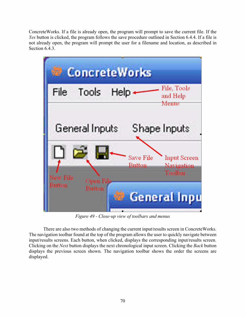
70

ConcreteWorks. If a file is already open, the program will prompt to save the current file. If the Yes button is clicked, the program follows the save procedure outlined in Section 6.4.4. If a file is not already open, the program will prompt the user for a filename and location, as described in Section 6.4.3.

Figure 49 - Close-up view of toolbars and menus

There are also two methods of changing the current input/results screen in ConcreteWorks. The navigation toolbar found at the top of the program allows the user to quickly navigate between input/results screens. Each button, when clicked, displays the corresponding input/results screen. Clicking on the Next button displays the next chronological input screen. Clicking the Back button displays the previous screen shown. The navigation toolbar shows the order the screens are displayed.

71

For more information on the printing features found in the File menu, see Section 6.4.1. See Section 6.4.6 for more information on the Tools menu and Section 6.4.7 for more information on the Help menu.

6.2. Inputs

6.2.1. Member Type

When a new file is selected, the user is prompted to select the type of member to analyze. In ConcreteWorks v2.0, the user may select from four basic types of concrete members: mass concrete, bridge decks, pavements, or precast beams. The analysis options available for each type of concrete member are shown in Table 1 of Chapter 1. The input screens available will depend on the type of member selected, and will only be shown if needed. For example, the Corrosion Inputs screen is not available when the user selects the Precast Concrete member type because ConcreteWorks does not contain a chloride service life module for precast beams. This manual will explain the inputs for all member types; note that if the input is not applicable for a particular member type, it will simply not be shown in the software. Additionally, the next and back buttons will show the next input screen available in the same order as the order of inputs shown in the input screen navigation toolbar shown in Figure 49.

6.2.2. General Inputs

The basic model settings and project inputs are all done in the General Inputs screen, as seen in Figure 50. The General Inputs screen is the first screen shown after opening a new or saved file, which is why there’s not a Back button shown. Changing the inputs in the General Inputs screen will fundamentally change other data entered later in the program. Changing the placement date, analysis duration, or project location will cause the weather data to change, even if maximum or minimum values have been entered earlier.

72

Figure 50 - General Inputs screen

Units

Many inputs in ConcreteWorks can be entered in either English units or Metric (S.I.) units. The English units system is the default units system in ConcreteWorks. When the system of units is changed, the program will prompt the user to change all values or cancel to stay in the current unit system. If the user chooses to change the values entered, the program assumes that the user entered the correct values for the old unit system, and will then multiply the entered values by the appropriate conversion factor for the new unit system. The Chloride Units input allows the user to select to perform the chloride service life calculations by % Chlorides by mass of concrete, or by mass per unit volume. The chloride surface concentration inputs in the Corrosion Inputs will be in the units chosen, as will the steel chloride threshold at corrosion initiation values, and the initial chloride concentration values.

Project Time and Date

The Placement Time box allows the user to enter the time concrete placement is started on the element being analyzed. If the cross section being analyzed is a horizontal cross section (such as a column), then the user should input the time concrete is placed at the particular cross section being analyzed. The default time is 7:00 a.m.

The Placement Date is entered by clicking on the number corresponding to the date of concrete placement. The month or year of placement can be changed by either clicking on the appropriate arrow or by clicking on the month or year. The default date is the current date.

Accurate results in ConcreteWorks depend on the user entering the correct time and date. Even if the minimum and maximum weather data is entered later in the program, the correct date

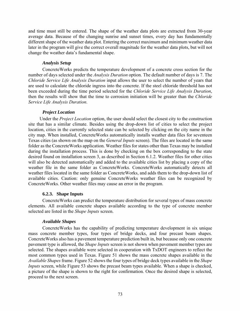
73

and time must still be entered. The shape of the weather data plots are extracted from 30-year average data. Because of the changing sunrise and sunset times, every day has fundamentally different shape of the weather data plot. Entering the correct maximum and minimum weather data later in the program will give the correct overall magnitude for the weather data plots, but will not change the weather data’s fundamental shape.

Analysis Setup

ConcreteWorks predicts the temperature development of a concrete cross section for the number of days selected under the Analysis Duration option. The default number of days is 7. The Chloride Service Life Analysis Duration input allows the user to select the number of years that are used to calculate the chloride ingress into the concrete. If the steel chloride threshold has not been exceeded during the time period selected for the Chloride Service Life Analysis Duration, then the results will show that the time to corrosion initiation will be greater than the Chloride Service Life Analysis Duration.

Project Location

Under the Project Location option, the user should select the closest city to the construction site that has a similar climate. Besides using the drop-down list of cities to select the project location, cities in the currently selected state can be selected by clicking on the city name in the city map. When installed, ConcreteWorks automatically installs weather data files for seventeen Texas cities (as shown on the map on the General Inputs screen). The files are located in the same folder as the ConcreteWorks application. Weather files for states other than Texas may be installed during the installation process. This is done by checking on the box corresponding to the state desired found on installation screen 3, as described in Section 6.1.2. Weather files for other cities will also be detected automatically and added to the available cities list by placing a copy of the weather file in the same folder as ConcreteWorks. ConcreteWorks automatically detects all weather files located in the same folder as ConcreteWorks, and adds them to the drop-down list of available cities. Caution: only genuine ConcreteWorks weather files can be recognized by ConcreteWorks. Other weather files may cause an error in the program.

6.2.3. Shape Inputs

ConcreteWorks can predict the temperature distribution for several types of mass concrete elements. All available concrete shapes available according to the type of concrete member selected are listed in the Shape Inputs screen.

Available Shapes

ConcreteWorks has the capability of predicting temperature development in six unique mass concrete member types, four types of bridge decks, and four precast beam shapes. ConcreteWorks also has a pavement temperature prediction built in, but because only one concrete pavement type is allowed, the Shape Inputs screen is not shown when pavement member types are selected. The shapes available were selected in cooperation with TxDOT engineers to reflect the most common types used in Texas. Figure 51 shows the mass concrete shapes available in the Available Shapes frame. Figure 52 shows the four types of bridge deck types available in the Shape Inputs screen, while Figure 53 shows the precast beam types available. When a shape is checked, a picture of the shape is shown to the right for confirmation. Once the desired shape is selected, proceed to the next screen.

74

Figure 51 - Shape Inputs screen for mass concrete member types

Figure 52 - Shape Inputs screen for bridge deck member types

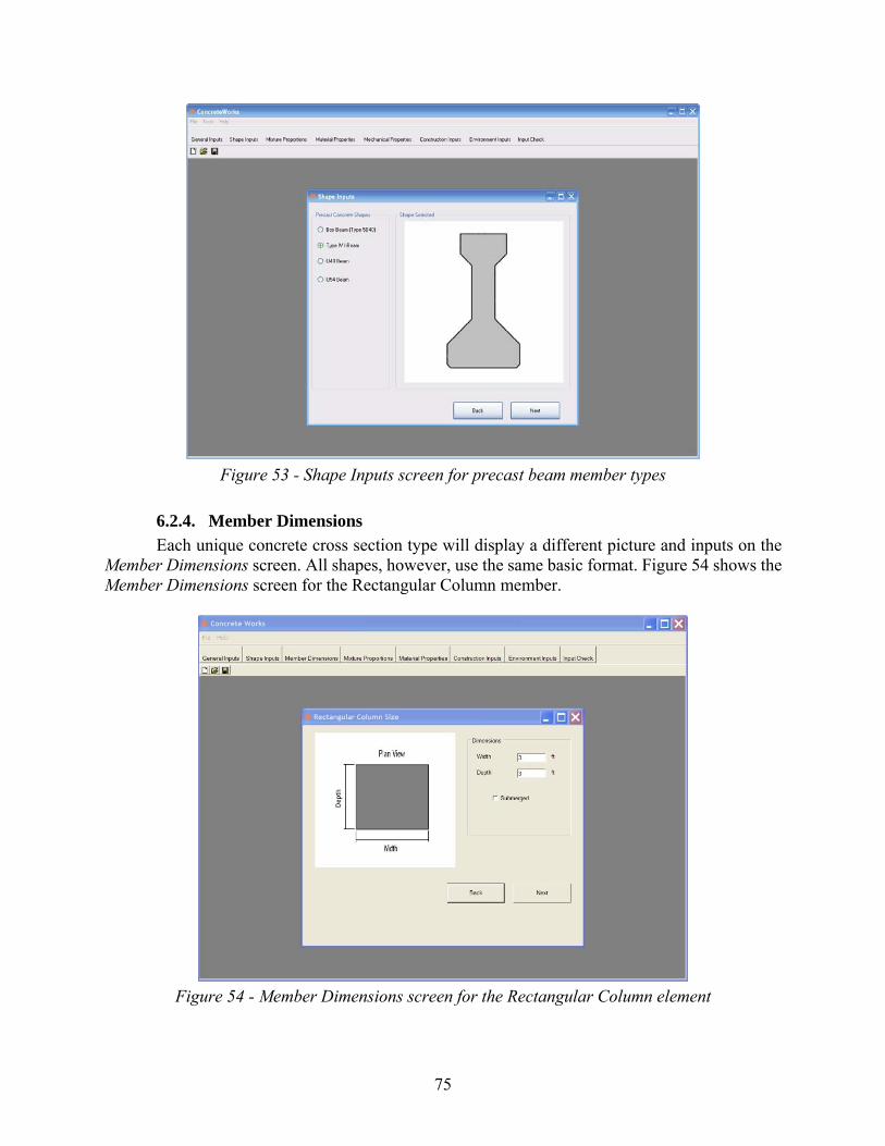
75

Figure 53 - Shape Inputs screen for precast beam member types

6.2.4. Member Dimensions

Each unique concrete cross section type will display a different picture and inputs on the Member Dimensions screen. All shapes, however, use the same basic format. Figure 54 shows the Member Dimensions screen for the Rectangular Column member.

Figure 54 - Member Dimensions screen for the Rectangular Column element

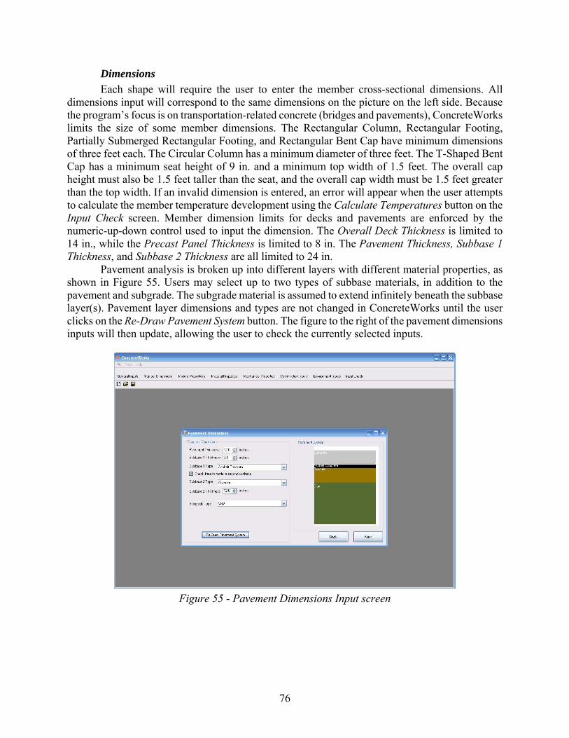
76

Dimensions

Each shape will require the user to enter the member cross-sectional dimensions. All dimensions input will correspond to the same dimensions on the picture on the left side. Because the program’s focus is on transportation-related concrete (bridges and pavements), ConcreteWorks limits the size of some member dimensions. The Rectangular Column, Rectangular Footing, Partially Submerged Rectangular Footing, and Rectangular Bent Cap have minimum dimensions of three feet each. The Circular Column has a minimum diameter of three feet. The T-Shaped Bent Cap has a minimum seat height of 9 in. and a minimum top width of 1.5 feet. The overall cap height must also be 1.5 feet taller than the seat, and the overall cap width must be 1.5 feet greater than the top width. If an invalid dimension is entered, an error will appear when the user attempts to calculate the member temperature development using the Calculate Temperatures button on the Input Check screen. Member dimension limits for decks and pavements are enforced by the numeric-up-down control used to input the dimension. The Overall Deck Thickness is limited to 14 in., while the Precast Panel Thickness is limited to 8 in. The Pavement Thickness, Subbase 1 Thickness, and Subbase 2 Thickness are all limited to 24 in.

Pavement analysis is broken up into different layers with different material properties, as shown in Figure 55. Users may select up to two types of subbase materials, in addition to the pavement and subgrade. The subgrade material is assumed to extend infinitely beneath the subbase layer(s). Pavement layer dimensions and types are not changed in ConcreteWorks until the user clicks on the Re-Draw Pavement System button. The figure to the right of the pavement dimensions inputs will then update, allowing the user to check the currently selected inputs.

Figure 55 - Pavement Dimensions Input screen

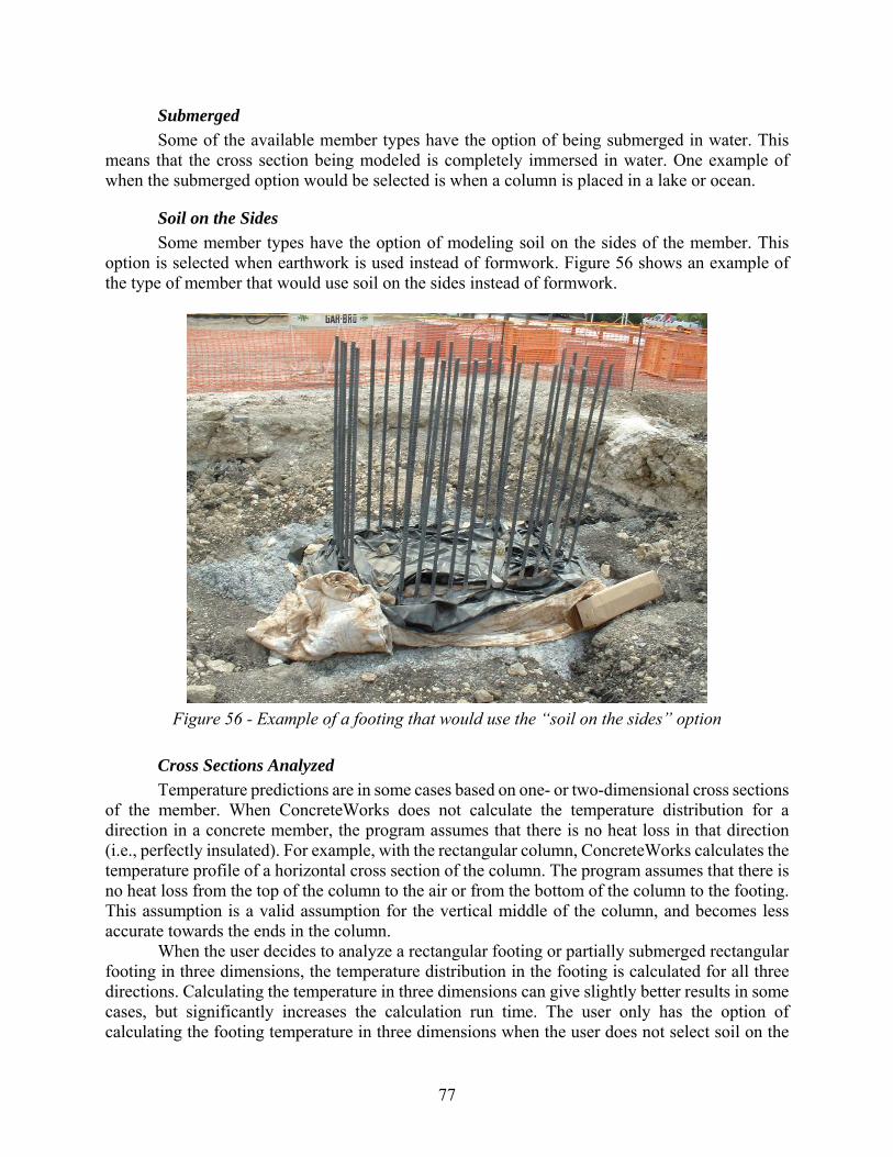
77

Submerged

Some of the available member types have the option of being submerged in water. This means that the cross section being modeled is completely immersed in water. One example of when the submerged option would be selected is when a column is placed in a lake or ocean.

Soil on the Sides

Some member types have the option of modeling soil on the sides of the member. This option is selected when earthwork is used instead of formwork. Figure 56 shows an example of the type of member that would use soil on the sides instead of formwork.

Figure 56 - Example of a footing that would use the “soil on the sides” option

Cross Sections Analyzed

Temperature predictions are in some cases based on one- or two-dimensional cross sections of the member. When ConcreteWorks does not calculate the temperature distribution for a direction in a concrete member, the program assumes that there is no heat loss in that direction (i.e., perfectly insulated). For example, with the rectangular column, ConcreteWorks calculates the temperature profile of a horizontal cross section of the column. The program assumes that there is no heat loss from the top of the column to the air or from the bottom of the column to the footing. This assumption is a valid assumption for the vertical middle of the column, and becomes less accurate towards the ends in the column.

When the user decides to analyze a rectangular footing or partially submerged rectangular footing in three dimensions, the temperature distribution in the footing is calculated for all three directions. Calculating the temperature in three dimensions can give slightly better results in some cases, but significantly increases the calculation run time. The user only has the option of calculating the footing temperature in three dimensions when the user does not select soil on the

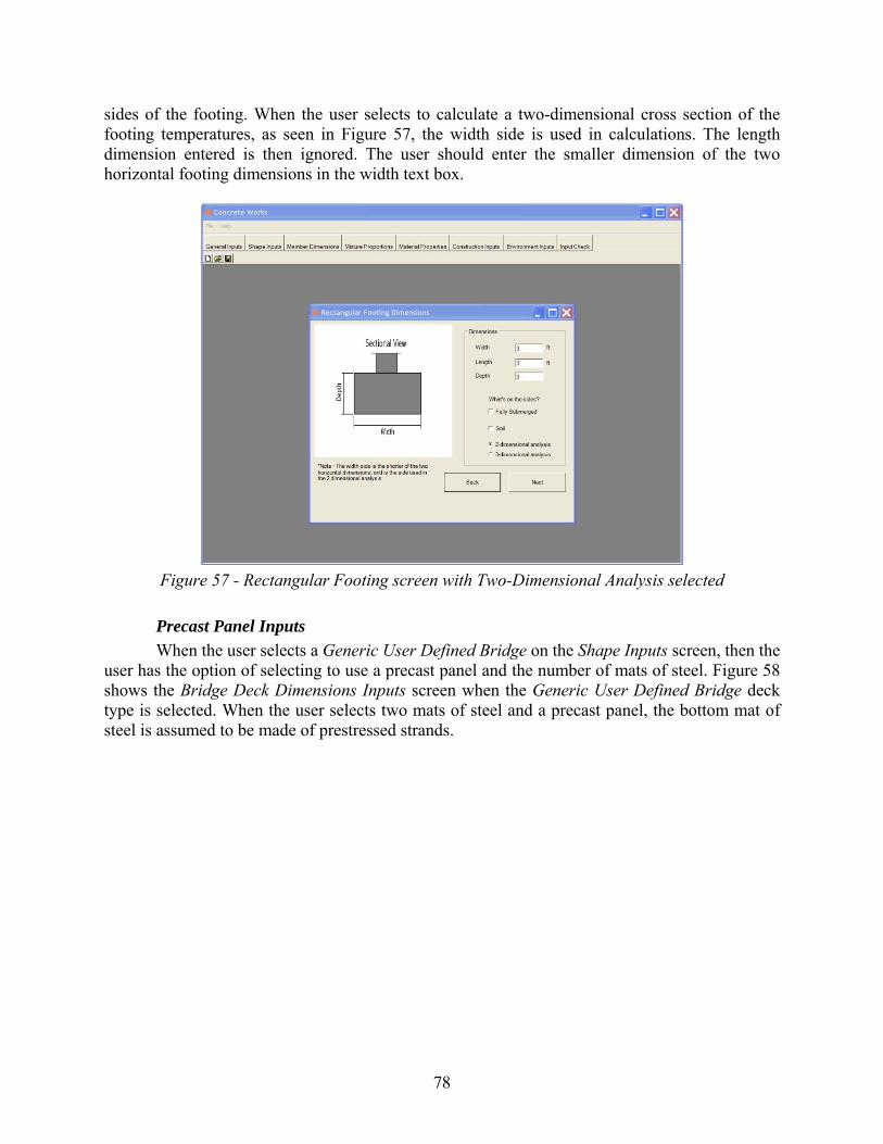
78

sides of the footing. When the user selects to calculate a two-dimensional cross section of the footing temperatures, as seen in Figure 57, the width side is used in calculations. The length dimension entered is then ignored. The user should enter the smaller dimension of the two horizontal footing dimensions in the width text box.

Figure 57 - Rectangular Footing screen with Two-Dimensional Analysis selected

Precast Panel Inputs

When the user selects a Generic User Defined Bridge on the Shape Inputs screen, then the user has the option of selecting to use a precast panel and the number of mats of steel. Figure 58 shows the Bridge Deck Dimensions Inputs screen when the Generic User Defined Bridge deck type is selected. When the user selects two mats of steel and a precast panel, the bottom mat of steel is assumed to be made of prestressed strands.

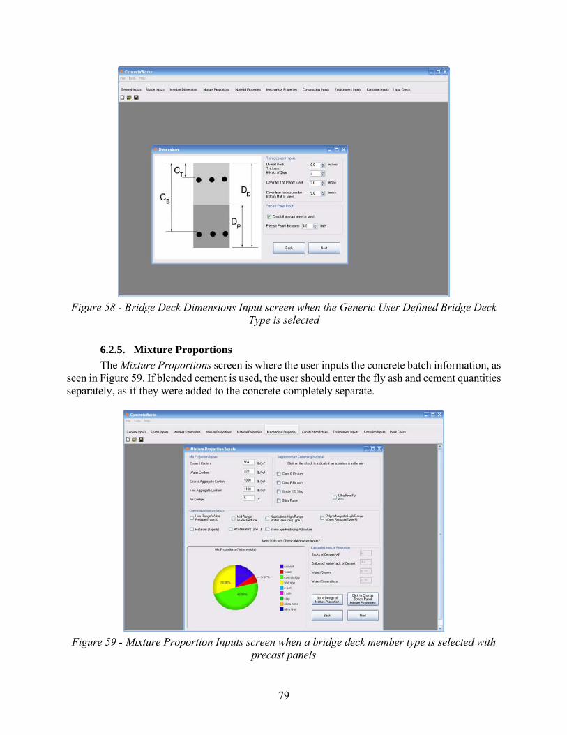
79

Figure 58 - Bridge Deck Dimensions Input screen when the Generic User Defined Bridge Deck

Type is selected

6.2.5. Mixture Proportions

The Mixture Proportions screen is where the user inputs the concrete batch information, as seen in Figure 59. If blended cement is used, the user should enter the fly ash and cement quantities separately, as if they were added to the concrete completely separate.

Figure 59 - Mixture Proportion Inputs screen when a bridge deck member type is selected with

precast panels

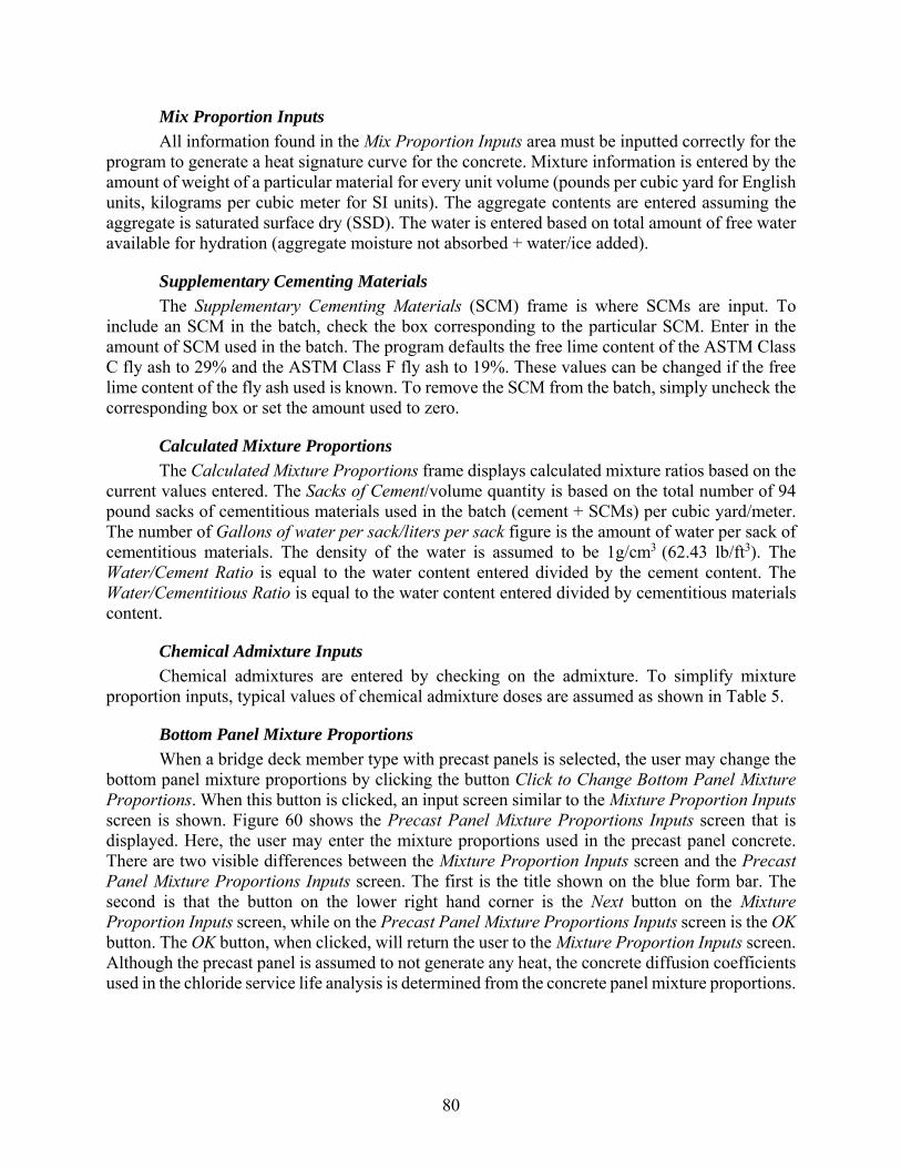
80

Mix Proportion Inputs

All information found in the Mix Proportion Inputs area must be inputted correctly for the program to generate a heat signature curve for the concrete. Mixture information is entered by the amount of weight of a particular material for every unit volume (pounds per cubic yard for English units, kilograms per cubic meter for SI units). The aggregate contents are entered assuming the aggregate is saturated surface dry (SSD). The water is entered based on total amount of free water available for hydration (aggregate moisture not absorbed + water/ice added).

Supplementary Cementing Materials

The Supplementary Cementing Materials (SCM) frame is where SCMs are input. To include an SCM in the batch, check the box corresponding to the particular SCM. Enter in the amount of SCM used in the batch. The program defaults the free lime content of the ASTM Class C fly ash to 29% and the ASTM Class F fly ash to 19%. These values can be changed if the free lime content of the fly ash used is known. To remove the SCM from the batch, simply uncheck the corresponding box or set the amount used to zero.

Calculated Mixture Proportions

The Calculated Mixture Proportions frame displays calculated mixture ratios based on the current values entered. The Sacks of Cement/volume quantity is based on the total number of 94 pound sacks of cementitious materials used in the batch (cement + SCMs) per cubic yard/meter. The number of Gallons of water per sack/liters per sack figure is the amount of water per sack of cementitious materials. The density of the water is assumed to be 1g/cm3 (62.43 lb/ft3). The Water/Cement Ratio is equal to the water content entered divided by the cement content. The Water/Cementitious Ratio is equal to the water content entered divided by cementitious materials content.

Chemical Admixture Inputs

Chemical admixtures are entered by checking on the admixture. To simplify mixture proportion inputs, typical values of chemical admixture doses are assumed as shown in Table 5.

Bottom Panel Mixture Proportions

When a bridge deck member type with precast panels is selected, the user may change the bottom panel mixture proportions by clicking the button Click to Change Bottom Panel Mixture Proportions. When this button is clicked, an input screen similar to the Mixture Proportion Inputs screen is shown. Figure 60 shows the Precast Panel Mixture Proportions Inputs screen that is displayed. Here, the user may enter the mixture proportions used in the precast panel concrete. There are two visible differences between the Mixture Proportion Inputs screen and the Precast Panel Mixture Proportions Inputs screen. The first is the title shown on the blue form bar. The second is that the button on the lower right hand corner is the Next button on the Mixture Proportion Inputs screen, while on the Precast Panel Mixture Proportions Inputs screen is the OK button. The OK button, when clicked, will return the user to the Mixture Proportion Inputs screen. Although the precast panel is assumed to not generate any heat, the concrete diffusion coefficients used in the chloride service life analysis is determined from the concrete panel mixture proportions.

81

Figure 60 - Precast Panel Mixture Proportions Inputs screen

6.2.6. Concrete Mixture Proportioning

If the user needs help with the concrete mixture design and proportioning, the user may click on the Go to Design of Mixture Proportion button on the lower right corner of the Mixture Proportions screen, as seen in Figure 59. The Design of Mixture Proportion screen will appear, as seen in Figure 61. The Design of Mixture Proportion screen guides the user through the mixture proportioning steps as found in ACI 211 (1991) and NHI Course 15123 (Hover, 2003). For a more detailed presentation of the mixture proportioning procedure and limitations, please refer to ACI 211 (1991) and Chapter 2 of this document. The most important thing to remember about the mixture proportion calculations is that they are only designed to create the proportions for making and testing a trial batch. The calculations in the Design of Mixture Proportions screen can never be used as a substitute for local knowledge of material properties or for trial batches. This is designed to be a user-friendly tool as the first step in designing mixtures for field applications.

The Cancel button on the Design of Mixture Proportion screen sends the user back to the Mix Proportions Inputs screen without any changes being made to the material weights. The OK button sends the user back to the Mixture Proportions Inputs screen, changing the material weights to those shown in the Final Volume Calculations. When a chemical admixture is checked in the Water Adjustment tab, the admixture is then checked on the Mix Proportions Inputs screen. When the High-Range Water Reducer (Type F) box is checked in the Design of Mixture Proportion screen, ConcreteWorks assumes that a Napthalene-based admixture is used.

82

Figure 61 - Design of Mixture Proportion screen—General Mix Information inputs

General Mix Information

The General Mix Information tab of the Design of Mixture Proportion screen displays all of the general material specifications. If not entered manually, the w/cm ratio is calculated from the Target Strength shown in the Strength Requirement frame, the air content, and any minimum w/cm ratios imposed by selecting a severe exposure condition from ACI 318-05 Tables 4.2.2 or 4.3.1.

The target strength is calculated by default on the specified f’c increased by the percent increase in target strength value. Alternatively, the user may calculate the concrete target strength by checking the box for using the concrete standard deviation, and then entering the standard deviation.

Aggregate Properties

The Aggregate Properties tab allows the user to either input the aggregate properties or calculated some of the inputs needed from an aggregate sieve analysis. Figure 62 shows the Aggregate Properties tab. Sieve Analysis Data for each aggregate type used should be entered as percent passing. Additionally, the percent of each aggregate used should be input as percent of the coarse or fine aggregate used, not the total amount of aggregates used. When the Update Agg. Properties button is clicked, the combined Coarse Aggregate Specific Gravity, combined Fine Aggregate Specific Gravity, and Maximum Size Aggregate inputs are updated. Additionally, the aggregate gradation charts are updated when the Update Agg. Properties button is clicked. An error is generated when the user enters a percent passing value that is larger than that from a larger size sieve, when the sum of coarse aggregate percent used values does not equal 100 percent, or when the sum of fine aggregate percent used values does not equal 100 percent. When the user checks the button that states Instead of ACI 211, optimize aggregate weights by:, the software will

83

calculate the aggregate amounts to use by optimizing the selected aggregate gradation index selected instead of the ACI 211 methods.

Figure 62 - Aggregate Properties tab on the Design of Mixture Proportions Inputs screen

Water Adjustment

The Water Adjustment tab contains tracking bars that let the user adjust the water requirements for the concrete by moving the tracking bar values, as seen in Figure 63. To use a water reducer, check the corresponding box on the Water Adjustment tab. Then move the track bar value to correspond to the water reduction gained from that particular admixture. The values used for maximum and minimum water reduction for all factors come from the NHI Course 15123 (Hover, 2003). A local knowledge of the water reduction properties for all the materials is extremely important. The quality of the concrete mixture designed will depend greatly on the accuracy of the inputs. Trial batches should always be made to verify the slump and strength properties of the concrete.

The Adjusted Water Content shown in the Paste Content frame is calculated based on the desired slump, the percent air, the aggregate gradation, and any water requirement adjustments made in the Water Adjustment tab (as described in Section 6.2.6). The cementitious material content is calculated by dividing the Adjusted Water Content by the w/cm ratio.

84

Figure 63 - Water Adjustment tab on the Design of Mixture Proportion screen

Final Volume Calculations

The final volume calculations for the concrete mixture are calculated based on the aggregate properties, cement content, adjusted water content, mineral admixture replacement, and air content. The batch weights per yard of concrete are shown in the Final Weights frame. The pie graph shows the percent of each material in the concrete mixture by volume. Figure 64 shows the Final Volume Calculations tab. When the total calculated paste content exceeds 30% by volume a warning appears to warn the user that the concrete mixture may be more susceptible to drying shrinkage. This does not preclude the use of the concrete mixture, but caution should be used for concrete members with a high surface area-to-volume ratio when exposed to low relative humidity.

85

Figure 64 - Final Volume tab of the Design of Mixture Proportion screen

6.2.7. Material Properties

The material characteristics are entered in the Material Properties screen. Figure 65 shows the Material Properties screen. To manually override the default cement chemistry and hydration parameters, check the corresponding boxes and enter in the desired values, as seen in Figure 66.

Figure 65 - Material Properties screen

86

Figure 66 - Material Inputs screen with manual adjustment checkboxes checked

Cement Chemical/Physical Properties

The Cement Chemical/Physical Properties frame is where the cement type, composition, and physical properties are entered. To change the cement properties to those for the cement used, check the Check to manually enter cement chemical/physical properties box. If the user unchecks the Check to manually enter cement chemical/physical properties box, the cement properties revert back to the default values for the cement type selected. When the Bogue method is selected under the Cement Analysis Method found in the Tools menu, the Bogue values and oxide contents for the cement properties are displayed. If the Rietveld method is selected instead of the Bogue method, then the cement composition phases corresponding to that method is displayed. Actual cement properties estimated using the Bogue method can be found on mill sheets shipped with the cement.

Hydration Calculation Properties

Hydration Calculation Properties are based on equations developed as part of TxDOT research project 0-4563, and are described in Section 3.1.5. Different models that describe the Hydration Calculation Properties are used depending on whether the Bogue method of the Rietveld method is used to define the cement properties. If the user has performed a semi-adiabatic calorimetry test on the concrete mixture used, then the calculated hydration properties can be changed by checking the Check to manually enter hydration properties box. When the Check to manually enter hydration properties box is checked, the hydration parameters do not change when the mixture proportions is changed or the cement type changes. The semi-adiabatic calorimetry test performed to determine hydration parameter equations for ConcreteWorks Version 2.0 came from mixes that used Texas materials. Low alkali cements were used in a majority of tests, and thus the hydration parameters for any mix containing a large amount of alkalis may not be as

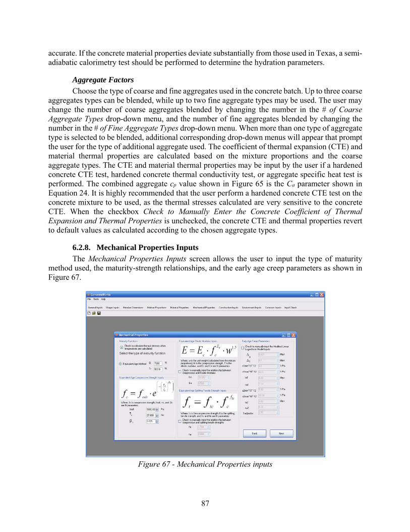
87

accurate. If the concrete material properties deviate substantially from those used in Texas, a semi-adiabatic calorimetry test should be performed to determine the hydration parameters.

Aggregate Factors

Choose the type of coarse and fine aggregates used in the concrete batch. Up to three coarse aggregates types can be blended, while up to two fine aggregate types may be used. The user may change the number of coarse aggregates blended by changing the number in the # of Coarse Aggregate Types drop-down menu, and the number of fine aggregates blended by changing the number in the # of Fine Aggregate Types drop-down menu. When more than one type of aggregate type is selected to be blended, additional corresponding drop-down menus will appear that prompt the user for the type of additional aggregate used. The coefficient of thermal expansion (CTE) and material thermal properties are calculated based on the mixture proportions and the coarse aggregate types. The CTE and material thermal properties may be input by the user if a hardened concrete CTE test, hardened concrete thermal conductivity test, or aggregate specific heat test is performed. The combined aggregate cp value shown in Figure 65 is the Ca parameter shown in Equation 24. It is highly recommended that the user perform a hardened concrete CTE test on the concrete mixture to be used, as the thermal stresses calculated are very sensitive to the concrete CTE. When the checkbox Check to Manually Enter the Concrete Coefficient of Thermal Expansion and Thermal Properties is unchecked, the concrete CTE and thermal properties revert to default values as calculated according to the chosen aggregate types.

6.2.8. Mechanical Properties Inputs

The Mechanical Properties Inputs screen allows the user to input the type of maturity method used, the maturity-strength relationships, and the early age creep parameters as shown in Figure 67.

Figure 67 - Mechanical Properties inputs

88

Maturity Functions

The Maturity Functions frame allows the user to select between the Nurse-Saul method of maturity and the Equivalent Age method, both as described in ASTM C 1074 (2004). For the Nurse-Saul method, a reference temperature of 0°C is used when metric units are selected and 0°F is used as the reference temperature when English units are selected. If the user has a maturity curve already calculated for the given concrete mixture, the user may enter the a and b strength parameters according to the equation shown on the Materials Inputs screen. The Check to calculate thermal stresses when temperatures are calculated checkbox must be checked for the software to calculate the concrete member cracking probability failure classification. When thermal stresses are to be calculated, the equivalent age maturity method must be used. The elastic modulus and splitting tensile strength equations are calculated from the concrete compressive strength fit parameters entered. At a minimum, the compressive strength/maturity relationship must be entered for the concrete mixture proportions and materials used. The accuracy of the thermal cracking probability analysis increases when the elastic modulus and splitting tensile strength are measured and input in the software.

Early Age Creep Parameters

The concrete early age creep is calculated using the Modified Linear Logarithmic Model (MMLM) described in Section 4.5. The early age creep parameters for the MLLM are calculated from the mixture proportions and material properties entered. Different equations are used, depending on whether the Bogue method or the Rietveld method is selected as described in Section 4.5.1.

6.2.9. Construction Inputs

The Construction Inputs screen is where the construction-related options are entered. Each type of concrete member will have different construction options to choose from. ConcreteWorks will automatically display the needed inputs based on the other options selected by the user, such as member type or whether the member is submerged. Do not be alarmed if a particular set of inputs does not appear with the particular choices made. If you change the member shape or submerged status, the available construction inputs will change. Even small mistakes, such as the form type, or blanket insulation, can yield dramatically different results. Figure 68 shows the Construction Inputs screen for a rectangular column.

89

Figure 68 - Construction Inputs screen for a rectangular column

Concrete Placement Temperature

The Estimated Placement Temperature is the temperature of the concrete when it arrives on the jobsite. The concrete placement temperature can be calculated three ways.

The first way is to click on the Calculate button. After it is clicked, the Raw Material Temperature Inputs screen will pop up. The temperature of the cementitious materials, aggregates, and water must be entered. Aggregate moisture contents and absorptions must also be entered. Optionally, ice may be entered if it is used in the batch. The OK button will not work until all of the required information is entered. After all of the required information is entered and the OK button is clicked, the calculated placement temperature will be displayed in the Estimated Placement Temperature box. ConcreteWorks uses the ACI 305 model for predicting the fresh concrete temperature (ACI 305R, 1991). When the Mixture Proportion inputs are changed, the predicted fresh concrete temperature will also change, if all of the required inputs are entered in the Raw Material Temperature Inputs screen. Note: if all of the required inputs in the Mixture Proportion Inputs screen are not entered, ConcreteWorks will not be able to calculate the fresh concrete temperature.

The second way is to calculate the concrete placement temperature from the ambient temperature. In this method, the concrete fresh temperature is estimated as the ambient temperature at the time of placement.

The third way to enter the concrete placement temperature is to check the Check here to manually enter Fresh Concrete Placement Temperature box. After the box has been checked, the user may enter the concrete placement temperature in the Estimated Placement Temperature box. If the Check here to manually enter Fresh Concrete Placement Temperature box is checked, the value in the Estimated Placement Temperature box will only change when manually entered by the user.

90

Formwork

The Concrete age at Form Removal input requires the user to input the concrete age when formwork is removed (at the cross section being analyzed), starting from the time the concrete was first mixed. The form type and form color must also be input in their corresponding boxes.

Surrounding Temperature

If the element selected is a footing or the element is submerged, the Construction Inputs screen will have inputs for the soil temperature and water temperature. The soil temperature refers to the average soil temperature for the time being modeled. A good estimate of the soil temperature for most footings is the average of the maximum and minimum ambient temperatures during the time period in question. The water temperature refers to the temperature of the water surrounding a concrete element. For example, if a column was being placed in a lake, the user would enter the average lake water temperature for that time period.

Curing Methods Applied after Forms Are Stripped

The After Forms Are Stripped area asks the user to input what kind of curing methods are applied to the member after the forms are removed. ConcreteWorks requires the user to enter a time in the box Time between form removal and curing method applied if a cure method is checked. If the user enters a delay time, but does not check a cure method box, ConcreteWorks assumes that no cure methods are used. The user cannot check both the Black Plastic option and the White or Clear Plastic option at the same time. If for some reason, both types of plastic are used in construction, the user should check the type of plastic used as the outside layer. All curing methods applied after forms are stripped are assumed to remain on the concrete member until the end of the analysis duration. The default time between removing forms and applying the cure method is one hour.

Footing Inputs

When a footing is selected as the member type, the Footing Inputs frame becomes visible on the Construction Inputs screen, as seen in Figure 69. The input Type of footing subbase asks the user to select the type of soil or rock on which the footing is built. If a plastic sheet is also used in curing, the user should select which color plastic is used. If both types of plastic are used, the user should select the color of the plastic placed on top. The input Concrete age when cure blanket is placed is the number of hours between concrete placement time and when cure methods are applied (the cure methods applied to the top before form removal). This input allows the concrete to set before placing the cure blankets on top of the footing.

If the sides of the footing are shaded from the sun because of scaffolding or the ground, the user should check the input Footing Sides Shaded.

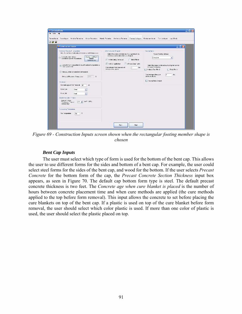
91

Figure 69 - Construction Inputs screen shown when the rectangular footing member shape is

chosen

Bent Cap Inputs

The user must select which type of form is used for the bottom of the bent cap. This allows the user to use different forms for the sides and bottom of a bent cap. For example, the user could select steel forms for the sides of the bent cap, and wood for the bottom. If the user selects Precast Concrete for the bottom form of the cap, the Precast Concrete Section Thickness input box appears, as seen in Figure 70. The default cap bottom form type is steel. The default precast concrete thickness is two feet. The Concrete age when cure blanket is placed is the number of hours between concrete placement time and when cure methods are applied (the cure methods applied to the top before form removal). This input allows the concrete to set before placing the cure blankets on top of the bent cap. If a plastic is used on top of the cure blanket before form removal, the user should select which color plastic is used. If more than one color of plastic is used, the user should select the plastic placed on top.

92

Figure 70 - Construction Inputs screen for a rectangular bent cap with pre-cast concrete

selected as the bottom form

Bridge Deck Inputs

ConcreteWorks assumes that a cure blanket is used on top of bridge decks. The user may additionally select to use a layer of plastic on top of blanket, the time the blanket is placed, and the concrete age when the cure blanket is removed. If wood forms are selected for the bridge deck, the user may additionally specify the concrete age at the wood form removal, as shown in Figure 71.

93

Figure 71 - Bridge Deck inputs when wood forms are selected

Precast Concrete Construction Inputs

Precast concrete members allow the user to specify a tarp or blanket to be used on the member sides. When a tarp or blanket is used on the sides of the precast beam, the same R-value is used for the blanket on the top and sides of the beam. The software also allows the user to select the subbase underneath the precast member, and the age when the cure method is started. The cure method is assumed to end when the forms are removed.

Pavement Construction Inputs

ConcreteWorks asks the user to input the type of cure method used as shown in Figure 72. The other pavement curing options depends on the curing method selected, and may ask the user for the application rate, the time of cure method application and removal, and the cure method color.

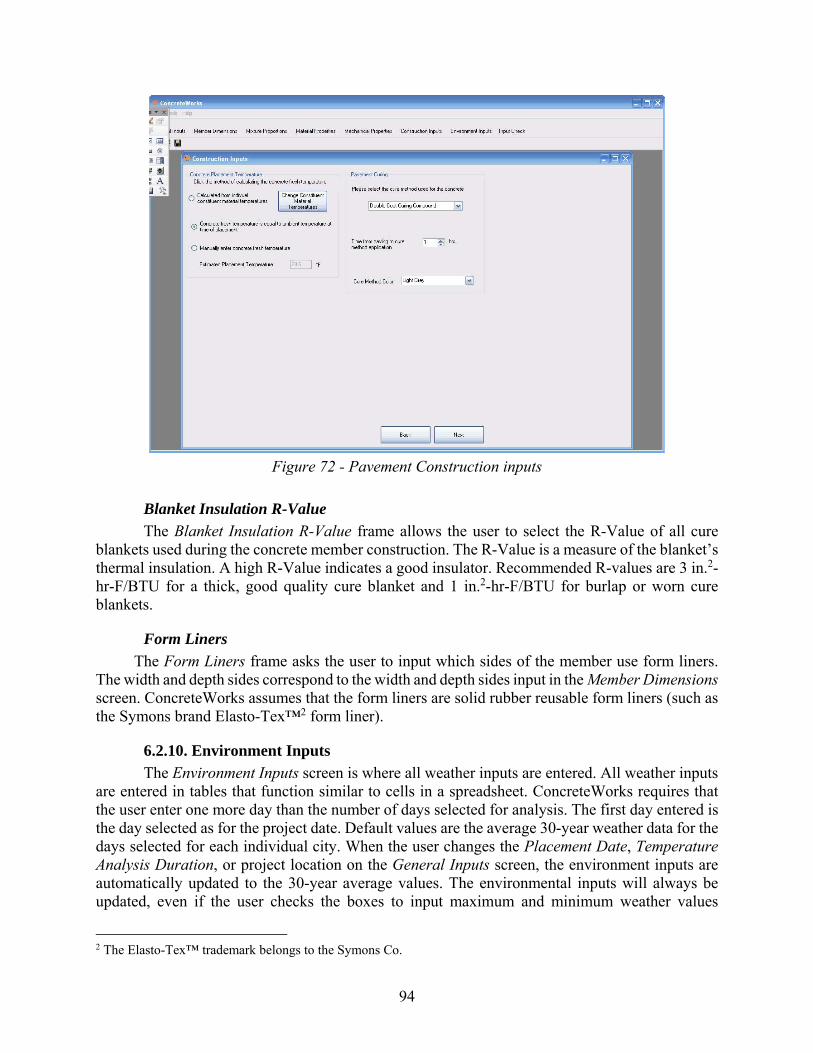
94

Figure 72 - Pavement Construction inputs

Blanket Insulation R-Value

The Blanket Insulation R-Value frame allows the user to select the R-Value of all cure blankets used during the concrete member construction. The R-Value is a measure of the blanket’s thermal insulation. A high R-Value indicates a good insulator. Recommended R-values are 3 in.2-hr-F/BTU for a thick, good quality cure blanket and 1 in.2-hr-F/BTU for burlap or worn cure blankets.

Form Liners

The Form Liners frame asks the user to input which sides of the member use form liners. The width and depth sides correspond to the width and depth sides input in the Member Dimensions screen. ConcreteWorks assumes that the form liners are solid rubber reusable form liners (such as the Symons brand Elasto-Tex™2 form liner).

6.2.10. Environment Inputs

The Environment Inputs screen is where all weather inputs are entered. All weather inputs are entered in tables that function similar to cells in a spreadsheet. ConcreteWorks requires that the user enter one more day than the number of days selected for analysis. The first day entered is the day selected as for the project date. Default values are the average 30-year weather data for the days selected for each individual city. When the user changes the Placement Date, Temperature Analysis Duration, or project location on the General Inputs screen, the environment inputs are automatically updated to the 30-year average values. The environmental inputs will always be updated, even if the user checks the boxes to input maximum and minimum weather values

2 The Elasto-Tex™ trademark belongs to the Symons Co.

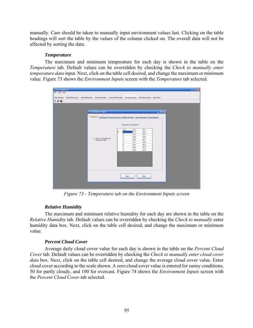
95

manually. Care should be taken to manually input environment values last. Clicking on the table headings will sort the table by the values of the column clicked on. The overall data will not be affected by sorting the data.

Temperature

The maximum and minimum temperature for each day is shown in the table on the Temperature tab. Default values can be overridden by checking the Check to manually enter temperature data input. Next, click on the table cell desired, and change the maximum or minimum value. Figure 73 shows the Environment Inputs screen with the Temperature tab selected.

Figure 73 - Temperature tab on the Environment Inputs screen

Relative Humidity

The maximum and minimum relative humidity for each day are shown in the table on the Relative Humidity tab. Default values can be overridden by checking the Check to manually enter humidity data box. Next, click on the table cell desired, and change the maximum or minimum value.

Percent Cloud Cover

Average daily cloud cover value for each day is shown in the table on the Percent Cloud Cover tab. Default values can be overridden by checking the Check to manually enter cloud cover data box. Next, click on the table cell desired, and change the average cloud cover value. Enter cloud cover according to the scale shown. A zero cloud cover value is entered for sunny conditions, 50 for partly cloudy, and 100 for overcast. Figure 74 shows the Environment Inputs screen with the Percent Cloud Cover tab selected.

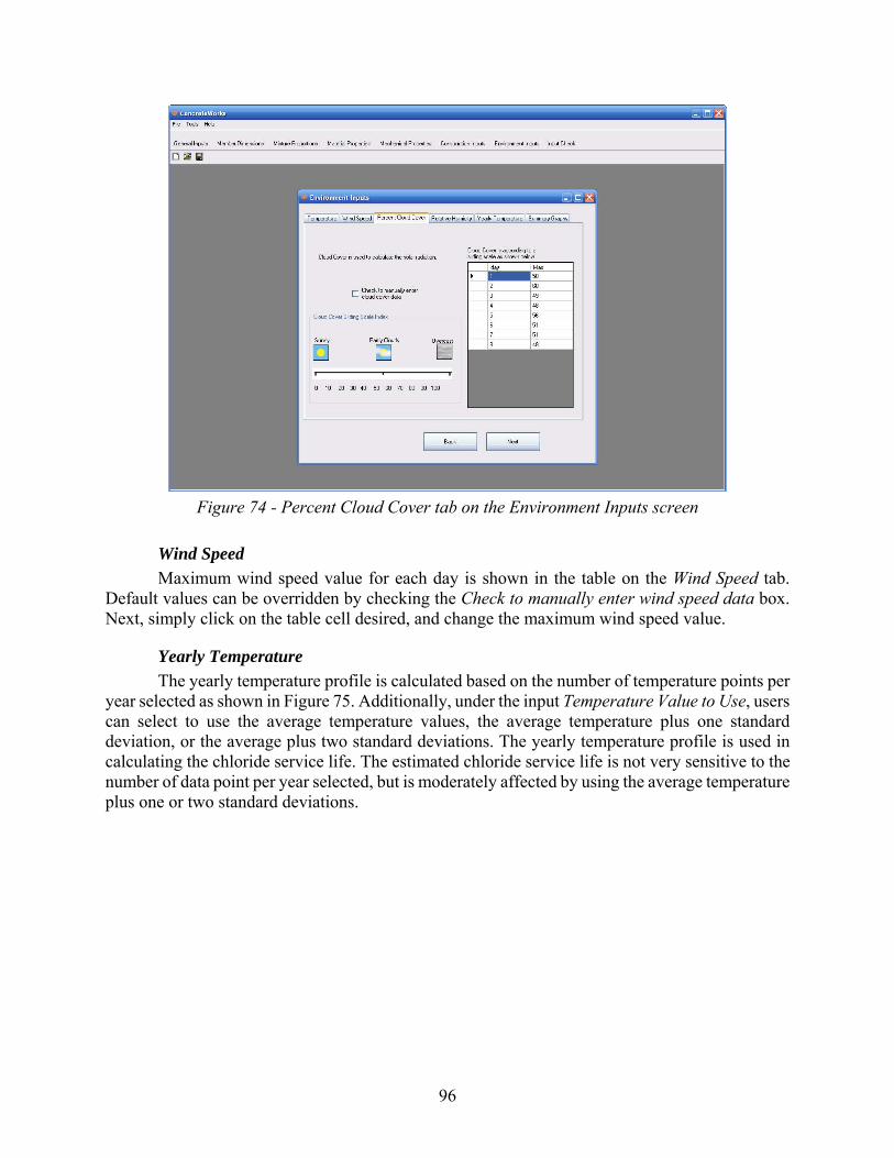
96

Figure 74 - Percent Cloud Cover tab on the Environment Inputs screen

Wind Speed

Maximum wind speed value for each day is shown in the table on the Wind Speed tab. Default values can be overridden by checking the Check to manually enter wind speed data box. Next, simply click on the table cell desired, and change the maximum wind speed value.

Yearly Temperature

The yearly temperature profile is calculated based on the number of temperature points per year selected as shown in Figure 75. Additionally, under the input Temperature Value to Use, users can select to use the average temperature values, the average temperature plus one standard deviation, or the average plus two standard deviations. The yearly temperature profile is used in calculating the chloride service life. The estimated chloride service life is not very sensitive to the number of data point per year selected, but is moderately affected by using the average temperature plus one or two standard deviations.

97

Figure 75 - Yearly Temperature inputs

Summary Graphs

The Summary Graphs tab can display the updated weather data on a graph. All plots start at 1:00 a.m. on the project date selected. The Temperature button shows a plot of temperature data with time. The Humidity button displays the relative humidity data with time. The Wind Speed tab shows a plot of wind speed with time. The Solar Radiation tab shows a plot of solar radiation with time. The solar radiation values are calculated based on the cloud cover data and relative humidity data. Figure 76 shows the Environment Inputs screen with the Summary Graphs tab selected. The graph shown in Figure 76 is a plot of the temperature.

98

Figure 76 - Summary Graphs tab on the Environment Inputs screen (the temperature graph is

currently displayed)

6.2.11. Input Check

The Input Check screen shows the values that have been entered, providing the user an opportunity to catch any mistakes made in the inputs section of ConcreteWorks. Anytime a user enters a character not allowed, ConcreteWorks assumes the value of the input to be zero. For example, if the user types “78u” on the Cement Content input in the Mixture Proportion Inputs screen, the Input Check screen would show that the cement content is “0”. Figure 77 shows the Input Check screen. Notice the default values are highlighted green, and the questionable values are highlighted red.

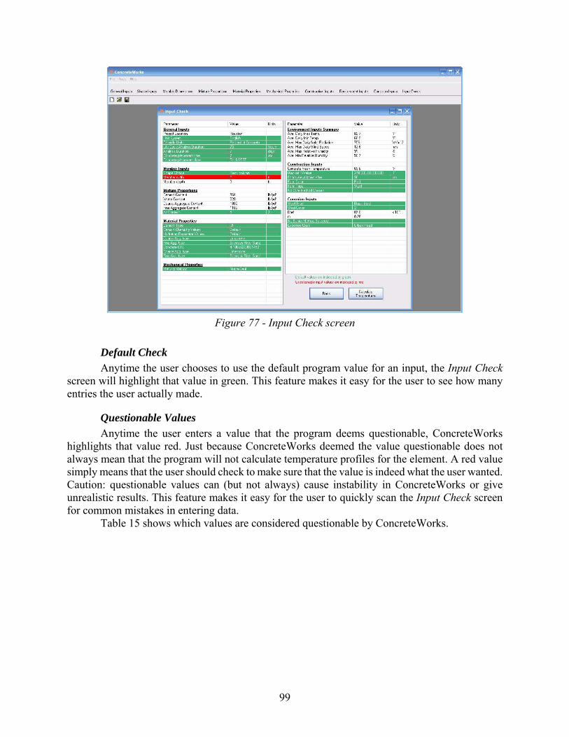
99

Figure 77 - Input Check screen

Default Check

Anytime the user chooses to use the default program value for an input, the Input Check screen will highlight that value in green. This feature makes it easy for the user to see how many entries the user actually made.

Questionable Values

Anytime the user enters a value that the program deems questionable, ConcreteWorks highlights that value red. Just because ConcreteWorks deemed the value questionable does not always mean that the program will not calculate temperature profiles for the element. A red value simply means that the user should check to make sure that the value is indeed what the user wanted. Caution: questionable values can (but not always) cause instability in ConcreteWorks or give unrealistic results. This feature makes it easy for the user to quickly scan the Input Check screen for common mistakes in entering data.

Table 15 shows which values are considered questionable by ConcreteWorks.

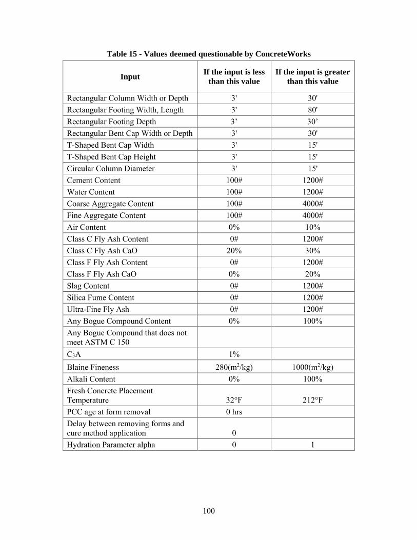
100

Table 15 - Values deemed questionable by ConcreteWorks

Input If the input is less

than this value If the input is greater

than this value

Rectangular Column Width or Depth 3' 30'

Rectangular Footing Width, Length 3' 80'

Rectangular Footing Depth 3’ 30’

Rectangular Bent Cap Width or Depth 3' 30'

T-Shaped Bent Cap Width 3' 15'

T-Shaped Bent Cap Height 3' 15'

Circular Column Diameter 3' 15'

Cement Content 100# 1200#

Water Content 100# 1200#

Coarse Aggregate Content 100# 4000#

Fine Aggregate Content 100# 4000#

Air Content 0% 10%

Class C Fly Ash Content 0# 1200#

Class C Fly Ash CaO 20% 30%

Class F Fly Ash Content 0# 1200#

Class F Fly Ash CaO 0% 20%

Slag Content 0# 1200#

Silica Fume Content 0# 1200#

Ultra-Fine Fly Ash 0# 1200#

Any Bogue Compound Content 0% 100%

Any Bogue Compound that does not meet ASTM C 150

C3A 1%

Blaine Fineness 280(m2/kg) 1000(m2/kg)

Alkali Content 0% 100%

Fresh Concrete Placement Temperature 32°F 212°F

PCC age at form removal 0 hrs

Delay between removing forms and cure method application 0

Hydration Parameter alpha 0 1

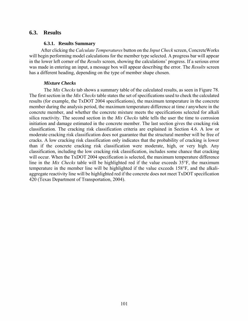
101

6.3. Results

6.3.1. Results Summary

After clicking the Calculate Temperatures button on the Input Check screen, ConcreteWorks will begin performing model calculations for the member type selected. A progress bar will appear in the lower left corner of the Results screen, showing the calculations’ progress. If a serious error was made in entering an input, a message box will appear describing the error. The Results screen has a different heading, depending on the type of member shape chosen.

Mixture Checks

The Mix Checks tab shows a summary table of the calculated results, as seen in Figure 78. The first section in the Mix Checks table states the set of specifications used to check the calculated results (for example, the TxDOT 2004 specifications), the maximum temperature in the concrete member during the analysis period, the maximum temperature difference at time t anywhere in the concrete member, and whether the concrete mixture meets the specifications selected for alkali silica reactivity. The second section in the Mix Checks table tells the user the time to corrosion initiation and damage estimated in the concrete member. The last section gives the cracking risk classification. The cracking risk classification criteria are explained in Section 4.6. A low or moderate cracking risk classification does not guarantee that the structural member will be free of cracks. A low cracking risk classification only indicates that the probability of cracking is lower than if the concrete cracking risk classification were moderate, high, or very high. Any classification, including the low cracking risk classification, includes some chance that cracking will occur. When the TxDOT 2004 specification is selected, the maximum temperature difference line in the Mix Checks table will be highlighted red if the value exceeds 35°F, the maximum temperature in the member line will be highlighted if the value exceeds 158°F, and the alkali-aggregate reactivity line will be highlighted red if the concrete does not meet TxDOT specification 420 (Texas Department of Transportation, 2004).

102

Figure 78 - Mix Checks tab shown on the Rectangular Column Temperature Model screen

Max-Min Graph

The Max-Min Graph tab shows the user a graph of the important calculated values with time, as seen in Figure 79. The values shown are the maximum temperature anywhere in the concrete member at each point in time, the minimum temperature anywhere in the concrete member at each point in time, the maximum temperature difference in the concrete member at each point in time, and the ambient temperature.

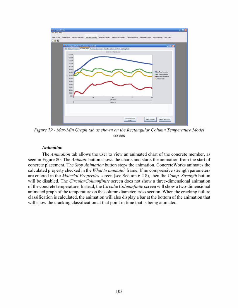
103

Figure 79 - Max-Min Graph tab as shown on the Rectangular Column Temperature Model

screen

Animation

The Animation tab allows the user to view an animated chart of the concrete member, as seen in Figure 80. The Animate button shows the charts and starts the animation from the start of concrete placement. The Stop Animation button stops the animation. ConcreteWorks animates the calculated property checked in the What to animate? frame. If no compressive strength parameters are entered in the Material Properties screen (see Section 6.2.8), then the Comp. Strength button will be disabled. The CircularColumnfinite screen does not show a three-dimensional animation of the concrete temperature. Instead, the CircularColumnfinite screen will show a two-dimensional animated graph of the temperature on the column diameter cross section. When the cracking failure classification is calculated, the animation will also display a bar at the bottom of the animation that will show the cracking classification at that point in time that is being animated.

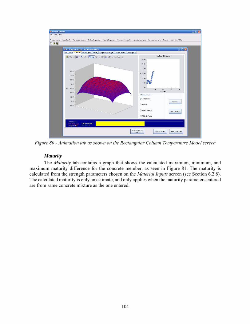
104

Figure 80 - Animation tab as shown on the Rectangular Column Temperature Model screen

Maturity

The Maturity tab contains a graph that shows the calculated maximum, minimum, and maximum maturity difference for the concrete member, as seen in Figure 81. The maturity is calculated from the strength parameters chosen on the Material Inputs screen (see Section 6.2.8). The calculated maturity is only an estimate, and only applies when the maturity parameters entered are from same concrete mixture as the one entered.

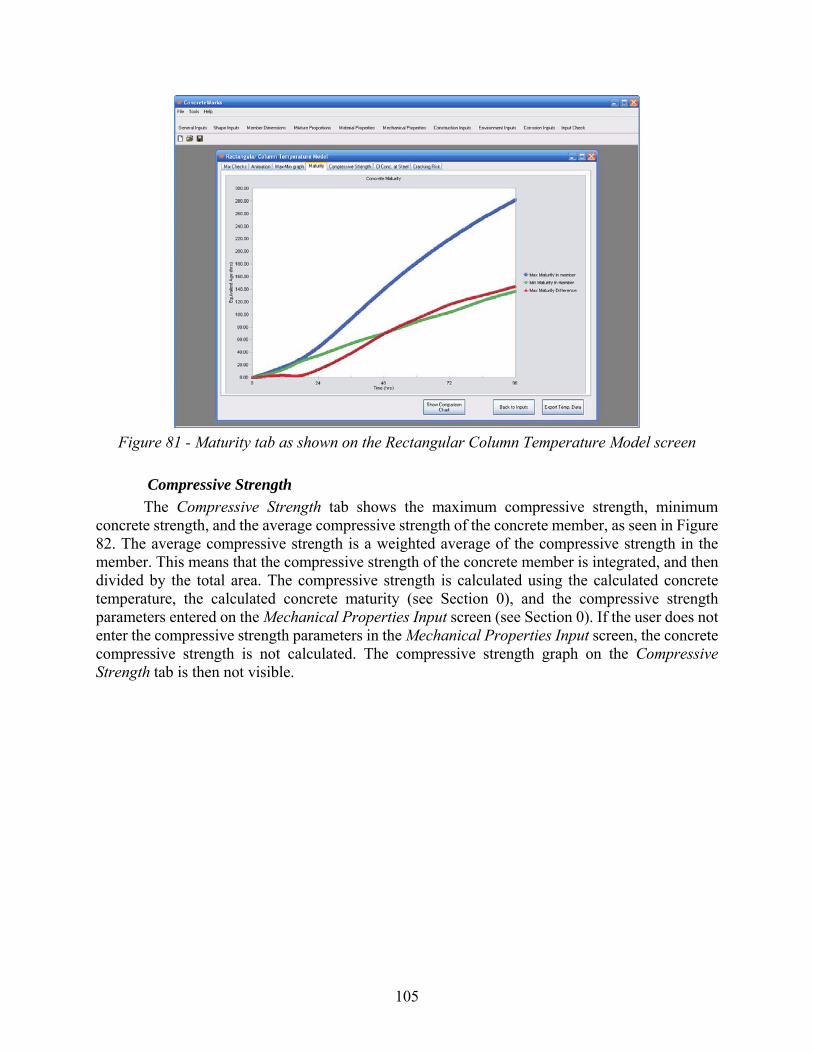
105

Figure 81 - Maturity tab as shown on the Rectangular Column Temperature Model screen

Compressive Strength

The Compressive Strength tab shows the maximum compressive strength, minimum concrete strength, and the average compressive strength of the concrete member, as seen in Figure 82. The average compressive strength is a weighted average of the compressive strength in the member. This means that the compressive strength of the concrete member is integrated, and then divided by the total area. The compressive strength is calculated using the calculated concrete temperature, the calculated concrete maturity (see Section 0), and the compressive strength parameters entered on the Mechanical Properties Input screen (see Section 0). If the user does not enter the compressive strength parameters in the Mechanical Properties Input screen, the concrete compressive strength is not calculated. The compressive strength graph on the Compressive Strength tab is then not visible.

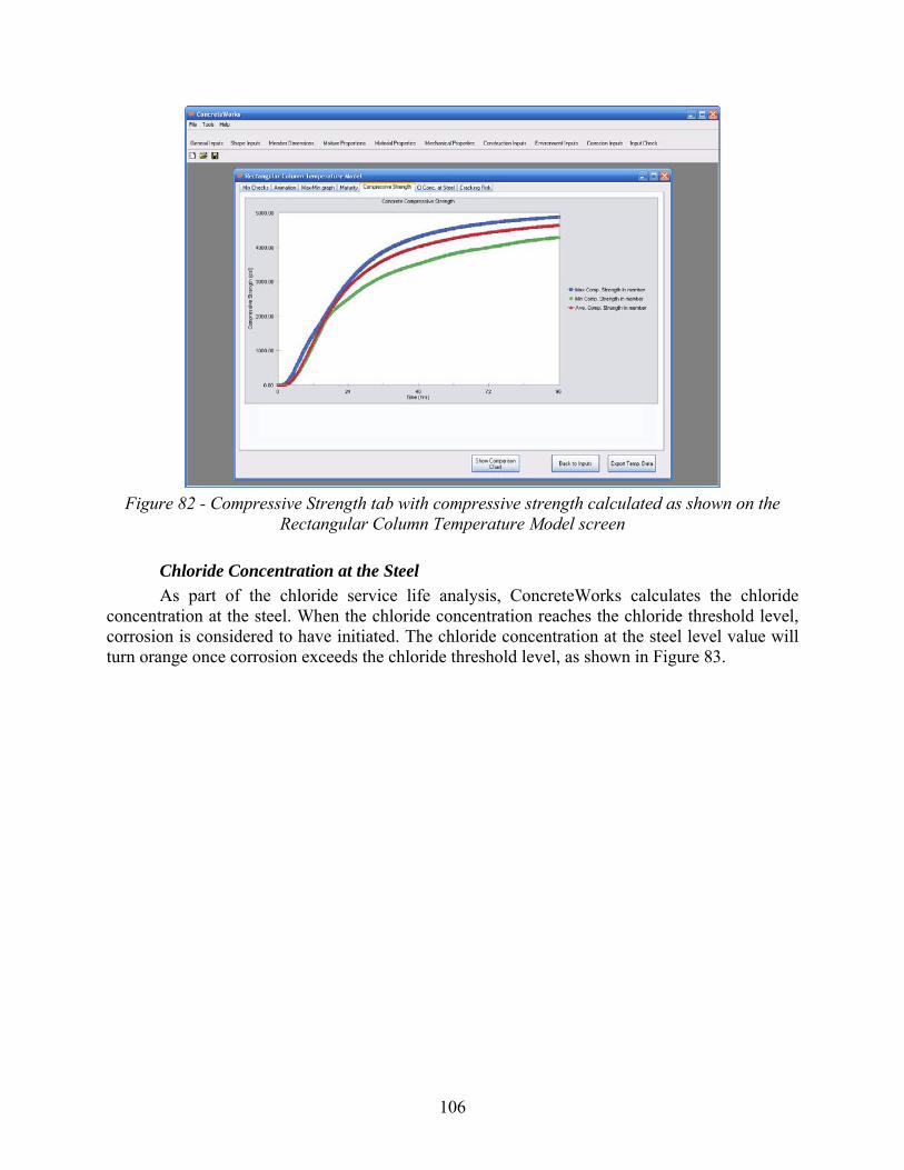
106

Figure 82 - Compressive Strength tab with compressive strength calculated as shown on the

Rectangular Column Temperature Model screen

Chloride Concentration at the Steel

As part of the chloride service life analysis, ConcreteWorks calculates the chloride concentration at the steel. When the chloride concentration reaches the chloride threshold level, corrosion is considered to have initiated. The chloride concentration at the steel level value will turn orange once corrosion exceeds the chloride threshold level, as shown in Figure 83.

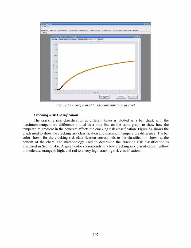
107

Figure 83 - Graph of chloride concentration at steel

Cracking Risk Classification

The cracking risk classification at different times is plotted as a bar chart, with the maximum temperature difference plotted as a blue line on the same graph to show how the temperature gradient in the concrete affects the cracking risk classification. Figure 84 shows the graph used to show the cracking risk classification and maximum temperature difference. The bar color shown for the cracking risk classification corresponds to the classification shown at the bottom of the chart. The methodology used to determine the cracking risk classification is discussed in Section 4.6. A green color corresponds to a low cracking risk classification, yellow to moderate, orange to high, and red to a very high cracking risk classification.

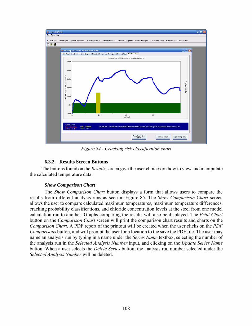
108

Figure 84 - Cracking risk classification chart

6.3.2. Results Screen Buttons

The buttons found on the Results screen give the user choices on how to view and manipulate the calculated temperature data.

Show Comparison Chart

The Show Comparison Chart button displays a form that allows users to compare the results from different analysis runs as seen in Figure 85. The Show Comparison Chart screen allows the user to compare calculated maximum temperatures, maximum temperature differences, cracking probability classifications, and chloride concentration levels at the steel from one model calculation run to another. Graphs comparing the results will also be displayed. The Print Chart button on the Comparison Chart screen will print the comparison chart results and charts on the Comparison Chart. A PDF report of the printout will be created when the user clicks on the PDF Comparisons button, and will prompt the user for a location to the save the PDF file. The user may name an analysis run by typing in a name under the Series Name textbox, selecting the number of the analysis run in the Selected Analysis Number input, and clicking on the Update Series Name button. When a user selects the Delete Series button, the analysis run number selected under the Selected Analysis Number will be deleted.

109

Figure 85 - Comparison chart screen

Export Temperature Data

To export the temperature data calculated, click on the Export Temperature Data button on the Results screen. ConcreteWorks saves the data in an ASCII text file when the extension .txt is used. ConcreteWorks will also save the data as an excel spreadsheet when the extension .xls is used. Data will be shown for discrete points in the member with time. The default file extension for data exported is “.xls”.

Cross Section to Be Displayed

ConcreteWorks only displays data in the graphs from two-dimensional cross sections. When a footing temperature distribution is calculated in three dimensions, the user may change which cross section is shown in the graphs by changing the Cross-Section Number to be Displayed value, and then clicking on the Display new cross-section button, as seen in Figure 86. The Mix Checks values are calculated for the full three-dimensional temperature distributions, however, and will not change when the Display new cross-section button is clicked. The temperature data exported when the Export Temperature Data button is clicked (as explained in Section 6.3.2) only exports the temperature data from the two-dimensional cross section currently selected.

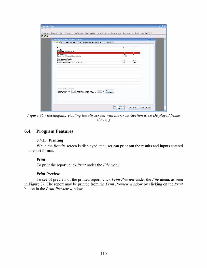
110

Figure 86 - Rectangular Footing Results screen with the Cross-Section to be Displayed frame

showing

6.4. Program Features

6.4.1. Printing

While the Results screen is displayed, the user can print out the results and inputs entered in a report format.

Print

To print the report, click Print under the File menu.

Print Preview

To see of preview of the printed report, click Print Preview under the File menu, as seen in Figure 87. The report may be printed from the Print Preview window by clicking on the Print button in the Print Preview window.

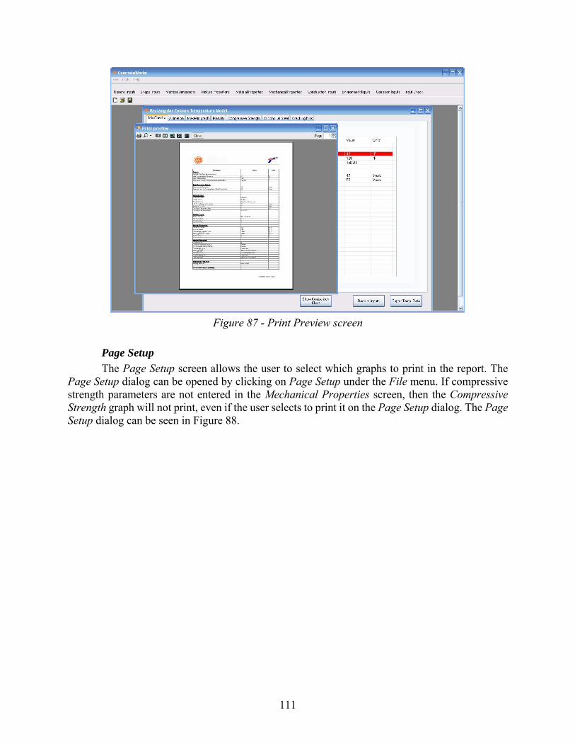
111

Figure 87 - Print Preview screen

Page Setup

The Page Setup screen allows the user to select which graphs to print in the report. The Page Setup dialog can be opened by clicking on Page Setup under the File menu. If compressive strength parameters are not entered in the Mechanical Properties screen, then the Compressive Strength graph will not print, even if the user selects to print it on the Page Setup dialog. The Page Setup dialog can be seen in Figure 88.

112

Figure 88 - Page Setup dialog

6.4.2. Export

The ConcreteWorks inputs and results can be exported to a PDF file. The PDF file exported is similar to the printed reports. To make the PDF report, select “PDF” from the “Export to” option under the File menu. The software will then prompt the user for a location to save the PDF file. It may take a few minutes for the software to generate the PDF file. After the file has been generated and saved, ConcreteWorks will display a message that the PDF file was generated.

ConcreteWorks also contains an option to export the inputs to SiteManager™. SiteManager™ is an AASHTOWare® product used by several state departments of transportation. The export to SiteManager™ function in ConcreteWorks will create an XML file that can be used to import ConcreteWorks inputs into SiteManager™.

6.4.3. Save As

To save the inputs entered in a new file, click Save As under the File menu. The default file extension for an inputs file is “.dat”.

6.4.4. Save File

To save a currently opened file, click the Save button, or click Save under the File menu. If the Save button is clicked and the file has not previously been saved, the program will prompt for a name and location.

6.4.5. Change Defaults

Click the Change Defaults item under the File menu to change the default values used for inputs to custom values. All values entered in the Change Defaults screen are input in English units, but are displayed in the correct units in the inputs section of ConcreteWorks the next time a

113

new file is opened. All units stay the same in the Change Defaults screen, except for the a and b strength parameters under the Mechanical Properties tab. The a and b parameters change units depending on the type of maturity function chosen under the same tab. The Material Inputs tab on the Change Defaults screen is seen on Figure 89.

Figure 89 - Material Inputs tab on the Change Defaults screen

6.4.6. Tools Menu

The Tools menu contains a few options that increase the power and versatility of ConcreteWorks. The first is the analysis method used to calculate the cement chemical properties. To select the Bogue method of determining the cement composition, select Bogue (ASTM C 150 2005) under the Cement Analysis Method under the Tools menu. To select the Rietveld method of determining the cement chemistry, select Rietveld under the Cement Analysis Method under the Tools menu. Different equations are used to determine the concrete heat of hydration and early age concrete creep properties based on the cement analysis method selected, as explained in Sections 3.1.5 and 4.5.1.

The specification used in the results check section can be changed by selecting the desired specification from the Specifications Used option under the Tools menu. ConcreteWorks currently only contains the 2004 specifications for the Texas Department of Transportation. If the Basic ASR and DEF specification is selected, ConcreteWorks will check to see if the predicted maximum temperature exceeds 160°F, and if the minimum amounts of SCMs prescribed by TxDOT in the 2004 specification are used. If the minimum amounts of SCMs are not used, then a warning that more investigations should be done is shown. Caution should be used in interpreting this check for alkali-silica reaction (ASR). Specifications that require the use of minimum amounts of supplementary cementing materials or maximum cement alkali levels to reduce the likelihood of ASR do not guarantee that this deleterious reaction will be prevented. Alkali silica reaction is

114

highly dependent on the aggregate type, type, and quantity of supplementary cementing materials, alkali loading, and exposure environment.

6.4.7. Help Menu

The Help menu provides the user with useful information about the ConcreteWorks program.

About ConcreteWorks

When the user clicks on the About ConcreteWorks item under the Help menu, a splash screen appears with information on the ConcreteWorks version being used, a link to the official ConcreteWorks website, www.texasconcreteworks.com, and a button that shows the End-User License Agreement. When the link to the official ConcreteWorks website is clicked, ConcreteWorks uses Internet Explorer® to navigate to the website—which is why Internet Explorer is required for using ConcreteWorks (as described in Section 6.1.2).

View User Manual

When the user clicks on the View User Manual item under the Help menu, the ConcreteWorks User Manual is opened as a new Adobe Reader® process (which is why Adobe Reader® is required for using ConcreteWorks, as described in Section 6.1.2).

6.5. Input Sensitivities

ConcreteWorks asks the user to input a great deal of data. To receive a correct answer, the user must enter correct data. Some of the data needed may be hard to obtain. Other data have less of an effect on the calculated results and performance of the model. This section contains some comments on these input sensitivities.

6.5.1. Environment Inputs Sensitivity

All of the Environment Inputs directly affect the way heat is transferred to or from the concrete member to the surrounding environment. Of the four types of environmental inputs, the temperature inputs have the greatest impact on the resulting temperature distribution in the element. The relative humidity and cloud cover inputs have a moderate effect on the data. A percent cloud cover value within 30% is generally acceptable. The wind data can also have a moderate effect on the calculated temperatures.

6.5.2. Run Speed

The run speed of the program is one of the biggest concerns to many designers. Following are the six factors that most influence the run speed of the program:

1. The computer speed and computer RAM

2. Analysis duration—A 14-day duration takes longer to run than a 5-day duration. When a thermal stress analysis is performed, the analysis duration has a very large impact on the run time. Because of the numerical methods used, an analysis duration of 4 days may have a run time several times that of a 3 day analysis, instead of the expected 33% longer runtime.

3. Member size—the larger the element, the longer the run-time.

115

4. Concrete age at form removal—the greater the time before form removal, the greater the run-time.

5. Cure method after form removal—if a cure blanket is used after form removal, the run-time is longer.

6. Three-dimensional analysis greatly increases the run-time compared to a two-dimensional analysis.

6.6. Troubleshooting

6.6.1. Installation Problems

If more than one version of the .NET Framework is installed, errors may occur during installation or when the ConcreteWorks is started. To resolve the issue, try deleting the folder containing the old version of the .NET Framework, usually found in the directory C:\WINDOWS\Microsoft.NET\Framework. Before installing or deleting any files or folders, make sure that the owner of the computer or appropriate network administrator is contacted to obtain permission and/or assistance.

6.6.2. Screen Settings

The screen settings on the computer running ConcreteWorks may adjust the program’s appearance. Some of the buttons may be cut off or not visible. The problem may be corrected by either manually resizing the program windows or adjusting the screen settings on the computer. To adjust the screen settings on the computer, open up the display settings window by right-clicking on the desktop. Then click on the Settings tab. Then adjust the screen resolution for optimal software viewing.

116

References

Abrams, D., 1918, “Effect of Time of Mixing on the Strength and Wear of Concrete,” ACI Journal Proceedings, Vol. 14, No. 6, pp. 22-92.

ACI 207.2, 1995, “Effect of restraint, volume change, and reinforcement on cracking in massive concrete,” American Concrete Institute, Farmington Hills, Mich., pp. 3-10.

ACI 209.2, 2008, “Guide for Modeling and Calculating Shrinkage and Creep in Hardened Concrete,” American Concrete Institute, Farmington Hills, Mich., pp. 20-22.

ACI 211, 1991, “Standard Practice for Selecting Proportions for Normal, Heavyweight, and Mass Concrete, ACI 211.1R, American Concrete Institute, Farmington Hills, Mich., 38 pp.

ACI 305R, 1991, “Hot Weather Concreting – Reported by ACI Committee 305,” American Concrete Institute, Farmington Hills, Michigan, 20 pp.

ACI 318, 2005, “Building Code Requirements for Structural Concrete (ACI 318-05) and Commentary (ACI 318R-05),” American Concrete Institute, Farmington Hills, Mich., pp. 99.

Al-Fadhala, M., and Hover, K.C., 2001, “Rapid Evaporation from Freshly Cast Concrete and the Gulf Environment,” Construction and Building Materials, Vol. 15, pp. 1-7.

Anson, M.; and Newman, K., 1966, "The effect of mix proportions and method of testing on Poisson's ratio for mortars and concretes," Magazine of Concrete Research, V. 18, No. 56, pp. 115-130.

ASHRAE, 1993, “1993-ASHRAE Handbook,” American Society of Heating, Refrigerating, and Air-Conditioning Engineers, Incorporated, Atlanta.

ASTM C 150, 2005, “Standard Specification for Portland Cement,” ASTM International, West Conshohocken, PA., 8 pp.

ASTM C 1074, 2004, “Standard Practice for Estimating Concrete Strength by the Maturity Method,” ASTM International, West Conshohocken, PA, 9 pp.

Barber, E.S., 1957, “Calculation of Maximum Pavement Temperatures from Weather Reports,” Bulletin 168, Highway Research Board, Washington, D.C., pp. 1-8.

Bažant, Z.P., and Panula, L., 1978, “Practical Prediction of Time-Dependent Deformations of Concrete Part IV: Temperature Effect on Basic Creep,” Matériaux et Constructions, Vol. 11, No. 66, pp. 424-434.

Bentz, E.C., and Thomas, M.D.A., 2001, “Life-365 Service Life Prediction Model™: User Manual,” 57 pp.

Bernard, O.; Ulm, F.; and Lemarchand, E., 2003, "A multiscale micromechanics-hydration model for the early-age elastic properties of cement-based materials," Cement and Concrete Research, V 33, pp. 1293–1309.

117

Bjøntegaard, O., 1999, "Thermal Dilation and Autogenous Deformation as Driving Forces to Self-Induced Stresses in High Performance Concrete," Doctoral Thesis, Division of Structural Engineering, The Norwegian University of Science and Technology, 256 pp.

Byard, B.E., 2011, “Early-Age Behavior of Lightweight Aggregate Concrete,” Doctoral Dissertation, Auburn University, 311 pp.

Byfors, J. 1980, “Plain Concrete at Early Ages,” Research 3:80, Swedish Cement and Concrete Research Institute, Stockholm, Sweden.

De Schutter, G, Taerwe, L., 1996, "Degree of hydration-based description of mechanical properties of early age concrete," Materials and Structures, V. 29, July, pp. 335-344.

Emanuel and Hulsey, 1977, “Prediction of the Thermal Expansion Coefficient of Concrete,” Journal of the American Concrete Institute, Vol. 74, No. 4, pp. 149-155.

Emborg, M., 1989, Thermal Stresses in Concrete Structures at Early Ages,” Doctoral Thesis, Luleå University of Technology, Division of Structural Engineering, 280 pp.

Emborg, M., 1998a, “Developing Early Age Mechanical Behaviour.” Rilem Report 15, Prevention of Thermal Cracking in Concrete at Early Ages, Edited by R. Springenschmid, E & Fn Spon, London, UK, pp. 76-148.

Emborg, M., 1998b, “Models and Methods for Computation of Thermal Stresses,” Prevention of Thermal Cracking in Concrete at Early Ages, Edited by R. Springenschmid, RILEM Report 15, EF Spon, London, pp 178-230.

Ge, Z., 2006, “Predicting Temperature and Strength Development of the Field Concrete,” Doctoral Dissertation, Iowa State University.

Glisic, B., 2000, "Fibre optic sensors and behaviour in concrete at early age," Doctoral Thesis, Swiss Federal Institute of Technology, Lausanne, Switzerland, 154 pp.

Hashida, H., and Yamazaki, N., 2002, “Deformation Composed of Autogenous Shrinkage and Thermal Expansion due to Hydration of High-Strength Concrete and Stress in Reinforced Structures,” Proceedings of the Third International Research Seminar on Self-Desiccation and its Importance in Concrete Technology, Edited by B. Persson and G. Fagerlund, Lund, Sweden, June 14-15, pp. 77-92.

Hedlund, H., 2000, “Hardening Concrete: Measurements and evaluation of non-elastic deformation and associated restraint stresses,” Doctoral Thesis, Luleå University of Technology, Division of Structural Engineering, 394 pp.

Hover, K., 2003, “NHI Course 15123 – Highway Materials Engineering: Portland Cement Concrete Module – Participant Workbook,”.

Hover, K.C., 2006, “Evaporation of Water from Concrete Surfaces,” ACI Materials Journal, Vol. 103, No. 5, pp. 384-389.

Incropera, F.P.; and Dewitt, D.P., 2002, Fundamentals of Heat and Mass Transfer, John Wiley & Sons, Inc., New York, p. 931.

Jensen, O.M.,and Hansen, P.F., 1999, "Influence of temperature on autogenous deformation and relative humidity change in hardening cement paste," Cement and Concrete Research, V 29, PP. 567-575.

118

Kada, H.; Lachemi, M.; Petrov, N.; Bonneau, O.; and Aïtcin, P.C., 2002, "Determination of the coefficient of thermal expansion of high performance concrete from initial setting," Materials and Structures, Vol. 35, No. 245, pp. 35-41.

Krauss, P.D.; Rogalla, E.A., 1996, “Transverse Cracking in Newly Constructed Bridge Decks,” NCHRP Report 380, Transportation Research Board, Washington, DC.

Larson, M., 2003, “Thermal Crack Estimation in Early Age Concrete – Models and Methods for Practical Application,” Doctoral Thesis, Division of Structural Engineering, Luleå University of Technology, 190 pp.

Lydon, F.D., and Balendran, R.V., 1986, “Some Observations on Elastic Properties of Plain Concrete,” Cement and Concrete Research, Vol. 16, No. 3, pp. 314-324.

Meyers, S.L., 1950, “Thermal Expansion Characteristics of Hardened Cement paste and of Concrete,” Proceedings, Highway Research Board, Vol. 30, pp. 193-203.

Mindess, S., Young, J.F., and Darwin, D., 2003, Concrete, 2nd Ed., Pearson Education, Inc., Upper Saddle River, NJ.

Mitchell, L.J., 1953, “Thermal Expansion Tests on Aggregates, Neat Cement, and Concretes,” Proceedings, ASTM, V. 53, pp. 963-977.

Oluokun, F.A., Burdette, E.G., and Deatherage, J.H., 1991, “Elastic Modulus, Poisson’s Ratio, and Compressive Strength Relationships at Early Ages,” ACI Materials Journal, Vol. 88, No. 1, pp. 3-10.

Patankar, S.V., 1980, Numerical Heat Transfer and Fluid Flow, McGraw-Hill Book Company, New York, p. 30-66.

Paulini, P., and Gratl, N., 1994, “Stiffness Formation on Early Age Concrete,” In Rilem Report 25, Thermal Cracking in Mass Concrete, E & FN Spon, London, pp. 153-160.

Poole, J.L., 2007, “Modeling Temperature Sensitivity and Heat Evolution of Concrete,” Doctoral Dissertation, The University of Texas at Austin, 299 pp.

Raphael, J.M., 1984, “Tensile Strength of Concrete,” ACI Journal, Vol. 81, No. 2, pp. 158-165.

Rietveld, H.M., 1969, “A Profile Refinement Method for Nuclear and Magnetic Structure,” Journal of Applied Crystallography, Vol. 2, pp. 65-71.

Riding, K.A., Poole, J.L., Schindler, A.K., Juenger, M.C.G., Folliard, K.J., 2007, “Temperature Boundary Condition Models for Concrete Bridge Members,” ACI Materials Journal, Vol. 104, No. 4, pp. 379-387.

Riding, K., 2007, “Early Age Concrete Thermal Stress Measurement and Modeling,” Doctoral Dissertation, The University of Texas at Austin, 588 pp.

RILEM Technical Committee 119-TCE, 1998, “Adiabatic and Semi-Adiabatic Calorimetry to Determine the temperature Increase in Concrete due to Hydration Heat of Cement,” RILEM Report 15, Prevention of Thermal Cracking in Concrete at Early Ages, Edited by R. Springenshmid, E & FN Spon, London, pp. 315-330.

Rostasy, F.S.; Gutsch, A.; and Laube, M., 1993, "Creep and Relaxation of Concrete at Early Ages - Experiments and Mathematical Modeling," Creep and Shrinkage of Concrete, Edited by Z.P. Bazant and I. Carol, E & Fn Spon, London, pp. 453-458.

119

Schindler, A.K., 2002, “Concrete Hydration, Temperature Development, and Setting at Early-Ages,” Doctoral Dissertation, The University of Texas at Austin, 530 pp.

Schindler, A.K., 2004, “Effect of Temperature on Hydration of Cementitious Materials”, ACI Materials Journal Vol. 101, No. 1, pp. 72-81.

Schindler, A.K., and Folliard, K.J., 2005, “Heat of Hydration Models for Cementitious Materials,” Vol. 102, No. 1, pp. 24-33.

Schöppel, K., and Springenschmid, R., 1994, “The Effect of Thermal Deformation, Chemical Shrinkage and Swelling on Restraint Stresses in Concrete at Early Ages,” RILEM Report 25, Thermal Cracking in Concrete at Early Ages, Edited by R. Springenschmid, E & FN Spon, London, UK, pp. 213-220.

Shilstone, J.M. Sr., and Shilstone, J.M. Jr., 2002, “Performance-Based Concrete Mixtures and Specifications for Today,” Concrete International, Vol. 24, No. 2, pp. 80-83.

TxDOT, 2004, “Special Provision 421 – Hydraulic Cement Concrete,” Texas Department of Transportation.

Tuthill, L., and Cordon, W.A., 1955, “Properties and Uses of Initially Retarded Concrete,” Journal of the American Concrete Institute, Vol. 27, No. 3, pp. 273-286.

Tuutti, K., 1982, “Corrosion of Steel in Concrete,” Swedish Cement and Concrete Research Institute, Report No. 4-82.

Van Breugel, K., 1998, “Prediction of Temperature Development in Hardening Concrete,” In Rilem Report 15, Prevention of Thermal Cracking in Concrete at Early Ages, Edited by R. Springenschmid, E & Fn Spon, London, pp. 51-75.

Viviani, M., 2005, “Monitoring and Modeling of Construction Materials During Hardening,” Doctoral Thesis, Swiss Federal Institute of Technology, Lausanne, Switzerland, 172 pp.

Walker, S., Bloem, D.L., and Mullen, W.G., 1952, “Effects of Temperature Changes on Concrete as Influenced by Aggregates,” Journal of the American Concrete Institute, Vol. 48, pp. 661-679.

Yamakawa, H., Nakauchi, H., Kita, T., and Onuma, H., 1986, “A Study of the Coefficient of Thermal Expansion of Concrete,” Transactions of the Japanese Concrete Institute, Vol. 8, pp. 111-118.

Yoshitake, I., Nagai, S., Tanimoto, T., and Hamada, S., 2002, “Simple Estimation of the Ground Water Temperature and Snow Melting Process,” Proceedings of The 11th Standing International Road Weather Commission, Sapporo, Japan, January 26-28, 8 pp.

0-6332-P2

CONCRETEWORKS SOFTWARE As of April 2017, this software is available on the TxDOT Engineering Software web page: http://www.txdot.gov/inside-txdot/division/information-technology/engineering-software.html