Conceptual spaces and semantic similarities of colors

Gerhard JagerUniversitat Tubingen, Seminar fur Sprachwissenschaft

Wilhelmstr. 19, 72074 Tubingen, Germanygerhard.jaeger@uni-tuebingen.de

Abstract

The paper presents a statistical evaluation of the typological data about color namingsystems across the languages of the world that have been obtained by the World ColorSurvey. In a first step, we discuss a singular value decomposition of the categorization datathat led to a small set of easily interpretable features dominant in color categorization.These features were used for a dimensionality reduction of the categorization data.

Using the thus preprocessed categorization data, we proceed to show that the availabletypological data support the hypothesis by the cognitive scientist Peter Gardenfors thatthe extension of color category are convex sets in the CIELab space in the languages ofthe world.

Keywords: color terms, conceptual spaces, semantic similarity, dimensionality reduction

1 Linguistic relativism and the semantics of color terms

The semantics of color terms, and the space of cross-linguistic variation regarding color se-mantics, has received a high amount of attention over the past decades. The domain of colorshas a fairly simple and well-understood structure. Also, basic color terms are usually simplemonomorphemic lexical entries. Still, relevant studies have unearthed interesting and non-trivial patterns of cross-linguistic variation. For these reasons, the semantics of color termshas been used as a paradigmatic case to address two fundamental issues: linguistic nativismand linguistic relativity.

The debate was initiated by the seminal study Berlin & Kay (1969). These authors in-vestigated the color vocabulary of 98 typologically distinct languages (20 of these languageswere studied in more detail). They found considerable variation in the size of basic colorvocabularies (where basic color terms were defined as morphologically simple color termswith unrestricted applicability, excluding loan words), ranging from three to eleven. How-ever, denotations of these terms were always drawn from a set of eleven universal categories(corresponding to the meanings of the English words black, white, red, green, yellow, blue,brown, gray, pink, purple, and orange). Furthermore they found that color term inventoriesfollow implicational universals of the type: “If a language has a word for yellow, it also hasa word for red.”

These results seem to indicate that the range of possible cross-linguistic semantic variationis severely constrained, arguably by non-linguistic aspects of perception and cognition. Thisargument was reinforced by the study Heider (1972). It provided evidence that the ability

1

of test persons to recognize and remember colors does not depend on their native language’scolor vocabulary.

This sparked a controversial discussion lasting to the present day. While some authorshave debated the existence of universal tendencies in color naming systems (e.g., Saunders& van Brakel 1997; Roberson et al. 2000), more recent results (such as Kay & Regier 2003;Lindsey & Brown 2006) have confirmed Berlin & Kay’s basic conclusions while suggestingmany modifications in detail. Also, some further experiments indicated that there is a cor-relation between the native languages of test persons and their ability to discriminate colorstimuli (Witthoft et al. 2003). Gilbert et al. (2006) argue that this correlation exists but isrestricted to the right visual field.

The present article studies the issue of the cross-linguistic universality of color namingsystems under a somewhat different perspective. It will be argued that across languages,color categories are convex regions of a universal conceptual space (in the sense of Gardenfors2000) of low dimensionality. The statistical techniques utilized in this context are inspiredby current work in computational distributional semantics (see for instance Erk 2012 for anoverview), thus suggesting a potential synergy between computational and cross-linguisticsemantics.

2 Semantic similarity and the geometry of meaning

It is a recurring thought in the history of natural language semantics that meanings aregeometrically structured in some way. The image schemas developed in cognitive semantics(Langacker 1987; Lakoff 1987; Talmy 1988) are an early example. Peter Gardenfors developeda full-blown program for semantic theory based on the idea that meanings are regions in someconceptual space which is endowed with a geometric structure (see for example especiallyGardenfors 2000; Gardenfors 2014).

Quite independently of these developments in cognitive linguistics, research on semanticsin quantitative natural language processing frequently employs geometric notions to representsemantic relations (see for instance Widdows 2004).

Utilizing geometric notions for semantic representations has several intuitively appealingaspects. The perhaps most attractive feature of this approach is the fact that the structure ofa semantic space can be derived from the pairwise similarities between semantic objects. Assimilarity judgments can be empirically determined in various ways, such as via psychologicalexperiments or corpus studies, the geometric approach offers an additional empirical foun-dation for semantic theory, complementing introspective judgments. Also, various meaningrelations such as synonymy, hyperonymy, relevance etc. can be given a geometric interpreta-tion. Furthermore, representing meanings geometrically allows to formulate semantic gener-alizations in geometrical terms not easily expressible in other frameworks. A case in point isGardenfors’ (2000) Criterion P :

“criterion p: A natural property is a convex region of a domain in a conceptualspace.”

Gardenfors (2000), 71

Together with Gardenfors’ assumption that simple adjectives denote natural properties,this leads to a semantic generalization that is not easily expressible in other semantic for-malisms.

2

3 Human color perception

The semantics of color terms is well-suited to spell out a geometrical approach to meaningbecause there is little controversy that the the conceptual domain in question — colors asperceived by humans — does have a geometrical structure, but identifying this structure isnon-trivial as it is not easily accessible to introspection.

Physiologically, human vision is based on photoreceptor cells in the retina sensitive tolight of various wave lengths and intensities. There are two types of such cells: cones respondto bright light while rods work best in dim lights. Only cones are able to differentiate wavelengths, i.e. colors. There are three types of cones sensitive to different wave lengths. Thethree types are specialized roughly to monochromatic red, green and blue light respectively(see for instance Bowmaker & Dartnalli 1980 for details). Connected to this is the factthat human color vision is three-dimensional. All perceivable colors can be arranged in athree-dimensional structure in such a way that the Euclidean distance between two colorsis inversely related to their perceived similarity. There are several three-dimensional colorspaces in use, depending on the desired technical or psychometric application. In this study,I will use the CIELab color space, a three-dimensional representation of colors that has beendesigned with the goal of perceptual uniformity. This means that equal distances within theCIELab space approximately corresponds to equal perceptual dissimilarity. The CIELab colorsolid is roughly spherically shaped. White and black are located at the North Pole and theSouth Pole respectively. The rainbow color are arranged around the equator. Lighter colors,such as bright yellow or pink, are located in the Northern hemisphere and darker colors, suchas brown or purple, in the Southern hemisphere. The various shades of gray are arrangedalong the earth’s axis.

As the domain of colors has a well-defined geometrical structure, it is well-suited to studythe predictions of the geometric theory of meaning. In this paper I will specificall be concernedwith Gardenfors’ claim that simple adjectives denote convex regions.

4 The World Color Survey

In their above-mentioned path-breaking study Berlin & Kay (1969), the authors investigatedthe color naming systems of 98 typologically distinct languages. They argued that there arestrong universal tendencies both regarding the extension and the prototypical examples forthe meaning of the basic color terms in these languages.

As mentioned in the introduction, this work sparked a controversial discussion. To counterthe methodological criticism that has been raised in this context, Kay and several co-workersstarted the World Color Survey project (WCS, see Cook et al. 2005 for details), a systematiclarge-scale collection of color categorization data from a sizeable amount of typologicallydistinct languages across the world.

The WCS researchers collected field research data for 110 unwritten languages, workingwith an average of 24 native speakers for each of these languages. During this investigation,the Munsell chips were used, a set of 330 chips of different colors that cover 322 colors ofmaximal saturation plus eight shades of gray. Figure 1 displays them in form of the Munsellchart.

The main chart is a 8 × 40 grid, with eight rows for different levels of lightness, and 40columns for different hues. Additionally there is a ten-level column of achromatic colors,

3

Figure 1: The Munsell chart

ranging from white via different shades of gray to black. The level of granularity is chosensuch that the difference between two neighboring chips is minimally perceivable.

For the WCS, each test person was “asked (1) to name each of 330 Munsell chips, shownin a constant, random order, and (2), exposed to a palette of these chips and asked to to pickout the best example(s) (‘foci’) of the major terms elicited in the naming task” (quoted fromthe WCS homepage). The data from this survey are freely available from the WCS homepagehttp://www.icsi.berkeley.edu/wcs/data.html.

This invaluable source of empirical data has been used in a series of subsequent evaluationsthat largely confirm Berlin and Kay’s hypothesis that there are universal tendencies in colornaming systems (see for instance Kay & Maffi 1999; Kay & Regier 2003; Regier et al. 2005,Lindsey & Brown 2006).

In the present study I will look primarily at structural commonalities in how the testpersons that participated in the WCS carve up the Munsell color space.

5 Cleaning up the data: dimensionality reduction

5.1 Motivation

For each informant, the outcome of the categorization task defines a partition of the Munsellspace into disjoint sets — one for each color term from their idiolect.

An inspection of the raw data reveals a certain level of noise. This may be illustratedwith the partitions of two speakers of a randomly chosen language (Central Tarahumara, anUto-Aztecan language spoken in Mexico). They are visualized in Figure 2.

In the figure, shades of gray and the shape of the points in the center of each cell representcolor terms of Central Tarahumara. We see striking similarities between the two speakers, butthe identity is not complete. They have slightly different vocabularies, and the extensions ofcommon terms are not identical. Furthermore, the boundaries of the extensions are unsharpand appear to be somewhat arbitrary at various places. Also, some data points seem to bedue to plain mistakes. Similar observations apply to the data from most informants.

Since the raw data from the WCS are quite noisy, in a first step I applied heuristicmethods to separate the linguistically/cognitively interesting variation in the data from noise.Techniques from distributional semantics proved to be suitable for this purpose.

Recall that the first task of the test persons in the World Color Survey was to name the330 Munsell chips, using color terms from their native languages. The outcome of this task

4

Figure 2: Partitions for two speakers of Central Tarahumara

can be represented as a contingency table. The rows of this matrix are word-language pairs,such as red/English or noir/French. (English and French are not covered in the WCS data,but they are used for illustrative purposes here.) There are 1,601 rows in total.

The columns of the contingency table are the 330 Munsell chips. Each cell contains thenumber of test persons that used the term corresponding to the row to name the Munsellchip corresponing to the color. The structure of this table is illustrated in Table 1. (The rownames and the numbers are made up for the purpose of illustration.)

A0 B0 B1 B2 · · · I38 I39 I40 J0

red/English 0 0 0 0 · · · 0 0 2 0green/English 0 0 0 0 · · · 0 0 0 0blue/English 0 0 0 0 · · · 0 0 0 0black/English 0 0 0 0 · · · 18 23 21 25white/English 25 25 22 23 · · · 0 0 0 0...

......

......

......

......

...rot/German 0 0 0 0 · · · 1 0 0 0grun/German 0 0 0 0 · · · 0 0 0 0gelb/German 0 0 0 1 · · · 0 0 0 0...

......

......

......

......

...rouge/French 0 0 0 0 · · · 0 0 0 0vert/French 0 0 0 0 · · · 0 0 0 0...

......

......

......

......

...

Table 1: Contingency table

This matrix is comparable to the term-document matrix (TDM) in distributional seman-tics (see for instance Widdows 2004: 145). A TDM is derived from a corpus which consistsof a selection of documents. It is a contingency matrix with terms as rows, documents ascolumns and the frequency of occurrence of a term in a document as entries.

5

The WCS contingency matrix can be seen as a collection of vectors in a 330-dimensionalspace. The 330 Munsell chips define the dimensions of this abstract space, and the usagepatterns of an individual term (of an individual languages) in the WCS gives a vector in this330-dimensional space.

In this representation, each vector (usage pattern of a term) has 330 degrees of freedom.It is for instance possible to represent a checkerboard pattern on the Munsell chart as suchvectors. However, we know that the color categorization patterns of human test persons aremuch more constrained — a checkerboard pattern is not a possible response of a WCS testperson. Let us assume that there are actually only k degrees of freedom in human colorcategorization, with k � 330. We want to project the raw data vectors from the contingencytable to a k-dimensional space while preserving as much information as possible.

5.2 Singular Value Decomposition in a nutshell

A commonly used method for this purpose (which also underlies the Latent Semantic Analysistechnique in distributional semantics; see Landauer & Dumais 1997) is based on SingularValue Decomposition (SVD). Let me illustrate the underlying intuition with a toy example.Remember the fairy tale of Hansel and Gretel. When the father leads the children into thewood for the first time, Hansel leaves a trail of pebbles along the way, which leads them backto their home after the parents abandoned them. Suppose they walked on a straight line, andthe pebbles are located as in the left panel of Figure 3.

Figure 3: Dimensionality reduction from two dimensions to one

Hansel did not manage to leave the pebbles exactly where they walked; their location intwo dimensions is perturbed by a certain amount of noise. To find back home, Hansel andGretel are interested to reconstruct the one-dimensional linear manifold that generated thepattern — the path they walked in the morning — and to filter out the uninformative noise.

SVD achieves this by finding a lower-dimensional linear manifold — a straight line — withthe property that its average distance to the observed points is minimized. This is shown inthe right panel of Figure 3. The white circles represent the projections of the observed datapoints onto the inferred lower-dimensional manifold.

6

While the toy example reduces dimensionality from two to one, the WCS data are pointsin a 330-dimensional space that should be projected onto a k-dimensional linear manifold, foran unkown value of k.

In the remainder of this subsection I will spell out the underlying mathematics of SVD, aswell as the postprocessing step applied, in somewhat more detail. This part can be skippedwithout loss of continuity.

There is a theorem of linear algebra which states that each matrix m × n M can bedecomposed in the following way (see for instance Strang 2009, Section 6.7):

M = UΣV T (1)

Here U is a m ×m orthogonal matrix, i.e. a rotation of points in m-dimensional space.Likewise, V is an n×n orthogonal matrix, i.e. a rotation of n-dimensional space. Σ is a m×ndiagonal matrix, i.e. a matrix where all entries except those on the main diagonal are zero.

The diagonal entries σi in Σ are the singular values of M . By convention, they are listedin descending order.

As explained above, the intuition underlying SVD is that there is an abstract space oflatent dimensions, and the variation of the data (represented by M) along the various latentdimensions is pairwise independent. The matrix U maps data points in an m-dimensionalspace (i.e. columns of M) onto the latent space. Likewise, U maps n-dimensional vectors(rows of M) onto the latent space. The singular value σi captures the importance of the i-thlatent dimension in distinguishing the data points in M .

When applied to the WCS contingency matrix, m is the number of term/language pairs(1,601) and n is the number of Munsell chips (330). The latent dimensions are, ideally, thecriteria test persons use when categorizing Munsell chips. Additionally, the WCS data havedegrees of freedem (i.e. latent dimensions) that reflect properties of the data collection processrather than cognitive features of color categorization. Let us assume, optimistically, that mostvariation in the WCS data reflect cognitively and linguistically meaningful information ratherthan noise due to data collection. Then there is a number k, with k � 330, such that thespace of the k most important latent dimensions captures the interesting variation in the data,while the remaining 330 − k latent dimensions reflect noise. Figure 4 displays the singularvalues of the WCS contingency table.

There is no fool-proof criterion to determine the number k of “interesting dimensions”.Figure 4 suggests that at most the first 20 latent dimension capture the relevant variation inthe data. In the sequel, I will — somewhat arbitrarly — choose k = 10. None of the resultsof this study depends on this choice though.

Let Σk be the result of replacing σi in Σ by zero for each i > k. If we replace Σ in equation(1) by Σk, we get

Mk = UΣkVT (2)

Mk is a matrix with the same shape as M . However, its rank is reduced to k, i.e. both itsrows and its columns are vectors within a k-dimensional linear manifold. In fact, Mk is therank-k matrix which is as close to M as possible.

Each of the 10 latent dimensions identified via SVD can be mapped to a vector of the330-dimensional space of Munsell chips. These vectors are the first 10 columns of the vectorV of equation (1). In Figure 5 the 3rd and 5th of these vectors are visualized for illustration.The values of a 330-dimensional vector along a dimension is represented by the shade of gray

7

0 50 100 150 200 250 300

050

010

0015

00

latent dimension

sing

ular

val

ue

Figure 4: Singular values of the WCS contingency table

of the corresponding position in the Munsell chart. White corresponds to the minimal andblack to the maximal value along any dimension.

As can be seen from these charts, the third latent dimension has its maximal values at redMunsell chips and its minimal values at white ones. So in short, this latent feature capturesthe contrast between white and red. Likewise, the 5th latent dimension captures the contrastbetween red and yellow. Similar — or more complex — patterns can also be discerned in theother eight latent dimensions.

The Varimax algorithm (Kaiser 1958) is a statistical technique to facilitate the inter-pretability of latent features. It amounts to a rotation of the latent (in our cases: 10-dimensional) subspace in such a way that the correlation of the latent with the observabledimensions is maximized. This procedure was applied to the 10-dimensional space resultingfrom SVD.

5.3 Results

The resulting 10 relevant dimensions, or features, are visualized in Figure 6. For each of thesefeatures, the high values are concentrated within a contiguous region of the Munsell chart.In most cases, these regions even correspond to the extension of English basic color terms:green, red, white, black, yellow, blue, purple, pink and brown. Only the 10th latent dimensionhas to be described with a non-basic term, light blue.

These findings indicate that the WCS test persons categorized Munsell chips mostly ac-cording to their degree of greenness, redness, whiteness etc. So the WCS data provide supportto Berlin and Kay’s claim that there are universal color categories that underlie the structureof the color vocabulary in typologically diverse languages.1

1The WCS data do not fully support Berlin and Kay’s more specific proposals about universals of colorvocabularies. These issues are discussed in detail in Jager (2012), using a methods similar to the ones describedhere.

8

J

I

H

G

F

E

D

C

B

A 1 2 3 4 5 6 7 8 9 10 11 12 13 14 15 16 17 18 19 20 21 22 23 24 25 26 27 28 29 30 31 32 33 34 35 36 37 38 39 40

J

I

H

G

F

E

D

C

B

A 1 2 3 4 5 6 7 8 9 10 11 12 13 14 15 16 17 18 19 20 21 22 23 24 25 26 27 28 29 30 31 32 33 34 35 36 37 38 39 40

Figure 5: Third and fifth latent dimension

The effect of mapping the raw data vectors to the 10 most important latent dimensions isillustrated in Figure 7. The first panel visualizes the row corresponding to the term aleluyafrom the Bolivian language Chiquitano. This term was only used by a single test person.That person used it for some, but not all, deep red Munsell chips. The vector that resultsfrom applying dimensionality reduction is shown in the second panel. It has high values forall red Munsell chips.

Another example is displayed in the third and fourth panel, representing the term madsmasof the Bantoid language Gunu (spoken in Cameroon). This term was used by two test person.One of them only used it to name two light gray Munsell chips, while the other one also appliedit to white and several whitish, very light blue and very light pink chips. After dimensionalityreduction (bottom panel), the corresponding vector has high values for white, all light shadesof gray and very light shades of blue and pink.

Dimensionality reduction can also be applied to the extension of a term as it is used by asingle test person. The set of chips which were categorized by the same term by a given testperson can be represented as a 330-dimensional binary vector. Let Vk be the matrix consistingof the first k columns of V . Vk can be conceived as a transformation that maps 330-dimensionalvectors (over Munsell chips) to k-dimensional vectors in the latent subspace. The matrix V T

k

represents a transformation that maps vectors from the k-dimensional latent space to an k-dimensional linear sub-manifold of the 330-dimensional Munsell space. Combining these twooperations to the matrix VkV

Tk is an operation within the 330-dimensional Munsell space that

supresses all but the first k latent dimensions. (The rows of Mk are the result of applying

9

Figure 6: Latent dimensions (Singular Value Decomposition + Varimax)

this operations to the corresponding rows or M .)To illustrate this, let us consider again the data from the first test person from the Mexican

language Central Tarahumara (cf. the upper panel of Figure 2). The upper left panel of Figure8 displays the extension of the term siyo. It covers almost all shades of green and blue, excepttwo single chips in the center of green and blue respectively. The upper right panel shows theextension of the term sita, which covers all shades of red plus the two green and blue outliers.The lower two panels visualize the result of applying dimensionality reduction to these twoextensions (or rather, their vector representation). The dimensionality-reduced version of siyonow covers all shades of blue and green, while sita is confined to all shades of red.

After dimensionality reduction, the values of the extension of a term for a single speakeris not binary anymore but contains values. It can be conceived as a fuzzy set with smoothboundaries.

For a given speaker, each Munsell chip c can be assigned to the term t for which c hasthe highest membership value after dimensionality reduction. This leads to a partition of

10

the Munsell space into disjoint categories. The net effect of this transformation is that theboundaries between categories are crisp but outliers in the raw data are removed. Figure 9displays the raw data for the first test person from Central Tarahumara (upper panel) andthe partition that results from dimensionality reduction (lower panel). Figure 10 displays theraw and the denoised partition for test person 11 from the Nilo-Saharan language Didinga(spoken in South Sudan). The comparison between the upper and the lower chart in bothfigures illustrates how dimensionality reduction smoothes the boundaries between categoriesand removes outliers.

6 Convexity in the CIELab space

6.1 Motivation

The visualizations that were discussed so far suggest the generalization that after dimension-ality reduction, category extensions are usually contiguous regions in the 2d Munsell space.This impression becomes even more striking if we study the extensions of categories in a geo-metrical representation of the color space with a psychologically meaningful distance metric.The CIELab space has this property. It is a 3d space with the dimension L* (for lightness),a* (the green-red axis) and b* (the yellow-blue axis). The set of perceivable colors forms athree-dimensional solid with approximately spherical shape. As described above, white is atthe North Pole, black at the South Pole, the rainbow colors form the equator, and the grayaxis cuts through the center of the sphere. The CIELab space has been standardized by theCommission Internationale d’Eclairage such that Euclidean distances between pairs of colorsare monotonically related to their perceived dissimilarity.

The 320 chromatic Munsell colors cover the surface of the color solid, while the ten achro-matic chips are located at the vertical axis. The color solid is actually not completely sphericalbut irregularly shaped.

Visually inspecting CIELab representations of the (dimensionality-reduced) partitions ledto the hypothesis that the boundaries between categories are in most cases linear, i.e. two-dimensional planes. This is in line with the main claim of Gardenfors’ (2000) book ConceptualSpaces. Gardenfors suggests that meanings can always be represented geometrically, and thatnatural categories must be convex regions in such a conceptual space. The three-dimensionalcolor space is one of his key examples.

In this section it will be tested to what degree this prediction is borne out for thedimensionality-reduced partitions obtained from the WCS. For this purpose, a computationalmethod was devised that modifies a partition (by re-categorizing individual Munsell chips) insuch a way that each category corresponds to a convex sub-region of the CIELab space andthese sub-regions do not overlap. The degree of convexity of a partition is the proportion ofMunsell chips that need to be re-categorized for convexification.

6.2 Finding convex approximations using Support Vector Machines

The convexification algorithm is described in more detail in this section. This material is notessential for the main thread of this article.

The algorithm can be described as follows. Suppose a partition p1, · · · , pk of the Munsellcolors into k categories is given.

11

1. For each pair of distinct categories pi, pj (with 1 ≤ i, j ≤ k), find a linear separatorin the CIELab space that optimally separates pi from pj . This means that the setof Munsell chips is partitioned into two linearly separable sets pi/j and pj/i, that arelinearly separable, such that the number of items in pi∩pj/i and in pj∩pi/j is minimized.

2. For each category pi, define

pi.=

⋂j 6=i

pi/j

As every pi/j is a half-space and thus convex, and the property of convexity is preserved underset intersection, each pi is a convex set.

To perform the linear separation in the first step, I used a soft-margin Support VectorMachine (SVM). An SVM (Vapnik & Chervonenkis 1974) is an algorithm that finds a linearseparator between two sets of labeled vectors in an n-dimensional space. An SVM is soft-margin if it tolerates misclassifications in the training data. As SVMs are designed to optimizegeneralization performance rather than misclassification of training data, it is not guaranteedthat the linear separators that are found in step 1 are really optimal in the described sense.Therefore the numerical results to be reported below provide only a lower bound for thedegree of success of Gardenfors’ prediction.

The output of this algorithm is a re-classification of the Munsell chips into convex sets(that need not be exhaustive). Figure 11 illustrates the convex approximation of a partitionwith the data of test person 12 from the Nilo-Saharan language Murle (spoken in South Sudanand Ethiopia). The upper panel shows the categorization performed by this test person afterdimensionality reduction. The lower panel gives the convex approximation of this partitionusing the procedure described above. It should be kept in mind that these charts are two-dimensional projections of the three-dimensional CIELab sapce. The region covering purpleand pink, for instance, is not convex in the projection. Nevertheless it does represent a convexregion in CIELab space.

It can be seen that there are minor differences between the two partitions concerningthe boundaries between adjacent categories. The five white squares in the lower chart markMunsell chips that could not uniquely be assigned to any convex category. In total the twopartitions agree for 306 out of 330 Munsell chips.

The degree of convexity “conv” of a partition is defined as the proportion of Munsell chipsthat are not re-classified in this process. If p(c) and p(c) are the class indices of chip c beforeand after re-classification, and if p(c) = 0 if c 6∈

⋃1≤i≤n pi, we can define formally:

conv.= |{c|p(c)=p(c)}|/330

For the example from Figure 11, this value is 306/330 ≈ 92.6%.

6.3 Results

The mean degree of convexity of the partitions that were obtained SVD and dimensionalityreduction is 93.8%, and the median is 94.5% (see the first boxplot in Figure 12).

One might wonder how important the dimensionality reduction step is in obtaining thisresult. To address this question, convex approximation via SVM training was also appliedto the raw partitions. Here the degree of convexity is only 77.9% (see the second boxplot inFigure 12).

12

Since the difference between these values is considerable, one might suspect that thehigh degree of convexity for the cleaned-up data is actually an artifact of the dimensionalityreduction algorithm and not a genuine property of the data. This is not very plausible,however, because the input for dimensionality reduction were exclusively categorization datafrom the WCS, while the degree of convexity depends on information about the CIELabspace. Nevertheless, to test this hypothesis, a random permutation of the category labelswas applied to each original partition. To the permuted data, the same analysis (SVD,dimensionality reduction, computation of the degree of convexity) was performed. The meandegree of convexity for these data is as low as 35.1% (see the third boxplot in Figure 12). Thefact that this value is so low indicates that the high average degree of convexity is a genuineproperty of natural color category systems and not a side effect of dimensionality reduction.

The choice of k = 10 as the number of relevant latent dimensions was somewhat arbitrary.Therefore it is important to test to what degree the results from this section depend on thischoice.

For this reason, the same analysis was performed with the original data for all values ofk between 5 and 20. The dependency of the mean degree of convexity on k is displayed inFigure 13. It can be seen that the degree of convexity is not very sensitive to the choice ofk. The highest value is achieved for k = 6 with mean degree of convexity of 94.3%. Forhigher values of k convexity slightly drops off, but at a slow rate. For k = 20, mean degreeof convexity is still at 92.8%. Most importantly, the mean degree of convexity only differsvery slightly (by less than 0.5%) between adjacent values of k. We can thus conclude thatthe choice of k does not seriously affect the qualitative conclusions of this study.

These results strongly indicate that color terms across typologically diverse languagesdenote convex regions within the CIELab space. This finding strongly supports Gardenfors’hypothesis that simple adjectives denote natural properties, which are, in turn, convex regionswithin some conceptual space.

7 Acknowledgments

I would like to thank the editors and reviewers of this volume for valuable feedback. Thisresearch has been supported by the ERC Advanced Grant 324246 EVOLAEMP (LanguageEvolution: The Empirical Turn) and the DFG-KFG 2237 Words, Bones, Genes, Tools, whichis gratefully acknowledged.

A Methods

Investigation where confined to the data from those informants for which the WCS containsa definite category term for each of the 330 Munsell chips. In total, 13,490 category exten-sions/vectors from 1,771 speakers from 102 languages (out of a total of 21,992 categories for2,616 speakers from 110 languages) have been used.

The convex approximations where computed by using the e1071 implementation (Dim-itriadou et al. 2005) of an SVM with a penalty term of 100 to minimize the number ofmisclassified training data rather than to maximize the margin.

13

References

Berlin, Brent, and Paul Kay. 1969. Basic color terms: their universality and evolution. Uni-versity of California Press: Berkeley and Los Angeles.

Bowmaker, James K., and Herbert J. A. Dartnall. 1980. ‘Visual pigments of rods and conesin a human retina’. The Journal of Physiology 298, 501–511.

Cook, Richard, Paul Kay, and Terry Regier. 2005. ‘The world color survey database: Historyand use’. In: Cohen, Henri, and Claire Lefebvre (eds.), Handbook of Categorisation in theCognitive Sciences. Amsterdam: Elsevier, 223–242.

Dimitriadou, Evgenia, Kurt Hornik, Friedrich Leisch, David Meyer, and Andreas Weingessel.2005. e1071: Misc Functions of the Department of Statistics (e1071). Tech. rep. Vienna:Technical University Vienna.

Erk, Katrin. 2012. ‘Vector space models of word meaning and phrase meaning: A survey’.Language and Linguistics Compass 6, 635–653.

Gardenfors, Peter. 2000. Conceptual Spaces. MIT Press: Cambridge, MA.Gardenfors, Peter. 2014. The Geometry of Meaning: Semantics Based on Conceptual Spaces.

MIT Press: Cambridge, MA.Gilbert, Aubrey L., Terry Regier, Paul Kay, and Richard B. Ivry. 2006. ‘Whorf hypothesis is

supported in the right visual field but not the left’. Proceedings of the National Academyof Sciences of the United States of America 103, 489–494.

Heider, Eleanor Rosch. 1972. ‘Universals in color naming and memory’. Journal of Experi-mental Psychology 93, 10–20.

Jager, Gerhard. 2012. ‘Using statistics for cross-linguistic semantics: a quantitative investiga-tion of the typology of color naming systems’. Journal of Semantics 29, 521–544.

Kaiser, Henry F. 1958. ‘The varimax criterion for analytic rotation in factor analysis’. Psy-chometrika 23, 187–200.

Kay, Paul, and Luisa Maffi. 1999. ‘Color appearance and the emergence and evolution of basiccolor lexicons’. American Anthropologist, 743–760.

Kay, Paul, and Terry Regier. 2003. ‘Resolving the question of color naming universals’. Pro-ceedings of the National Academy of Sciences 100, 9085–9089.

Lakoff, George. 1987. Women, fire, and dangerous things: What categories reveal about themind. University of Chicago Press: Chicago.

Landauer, Thomas K., and Susan T. Dumais. 1997. ‘A Solution to Plato’s problem: thelatent semantic analysis theory of acquisition, induction and representation of knowledge’.Psychological Review 104, 211–240.

Langacker, Ronald Wayne. 1987. Foundations of Cognitive Grammar. Vol. 1. Stanford Uni-versity Press: Stanford.

Lindsey, Delwin T., and Angela M. Brown. 2006. ‘Universality of color names’. Proceedingsof the National Academy of Sciences 103, 16608–16613.

Regier, Terry, Paul Kay, and Richard S. Cook. 2005. ‘Focal colors are universal after all’.Proceedings of the National Academy of Sciences 102, 8386–8391.

Roberson, Debie, Ian R. L. Davies, and Jules Davidoff. 2000. ‘Color categories are not uni-versal: Replications and new evidence from a Stone-age culture’. Journal of ExperimentalPsychology: General 129, 369–398.

Saunders, Barbara A. C., and Jaap van Brakel. 1997. ‘Are there nontrivial constraints oncolour categorization?’ Behavioral and Brain Sciences 20, 167–228.

Strang, Gilbert. 2009. Introduction to Linear Algebra. Wellesley-Cambridge Press: Wellesley.

14

Talmy, Leonard. 1988. ‘Force dynamics in language and cognition’. Cognitive Science 12, 49–100.

Vapnik, Vladimir, and Alexey Chervonenkis. 1974. Theory of pattern recognition [in Russian].Nauka: Moscow.

Widdows, Dominic. 2004. Geometry and meaning. CSLI Publications: Stanford.Witthoft, Nathan, Jonathan Winawer, Lisa Wu, Michael Frank, Alex Wade, and Lera Borodit-

sky. 2003. ‘Effects of language on color discriminability’. In: Proceedings of the 25th AnnualMeeting of the Cognitive Science Society.

Biographical note

Gerhard Jager obtained his PhD at Humboldt-University in Berlin in 1996. He becameprofessor of semantics in syntax at Bielefeld University in 2004. Since 2009 he is professor ofgeneral linguistics in Tubingen.

He has worked on a variety of topics in semantics and mathematical linguistics, includingdynamic semantics, categorial grammar, and Optimality Theory. In recent years his researchhas mostly focused on evolutionary and game theoretic approaches to the dynamics of lan-guage.

15

Figure 7: The effect of dimensionality reduction

16

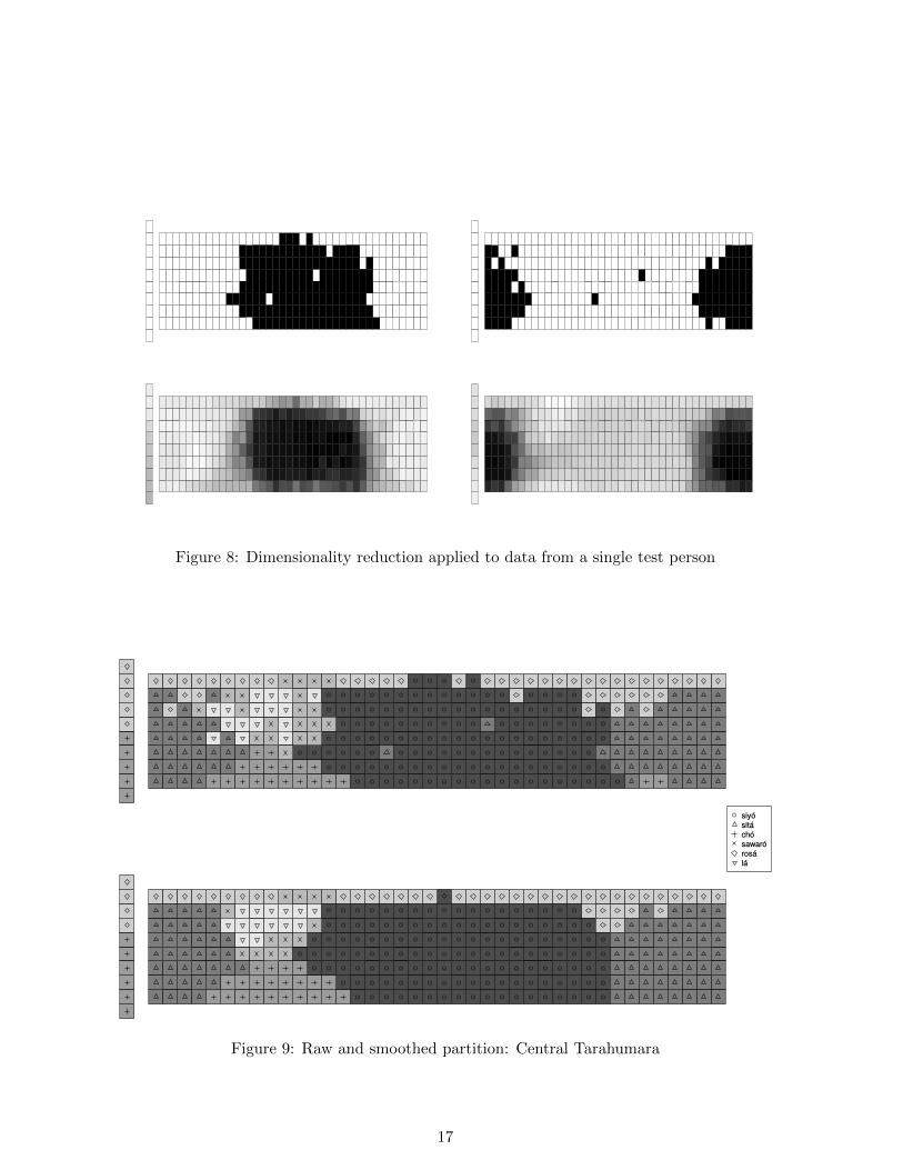
Figure 8: Dimensionality reduction applied to data from a single test person

Figure 9: Raw and smoothed partition: Central Tarahumara

17

Figure 10: Raw and smoothed partition: Didinga

Figure 11: Convex approximation of a partion: an example from Murle

18

●●●

●

●●●●●

●

●

●

●

●●

●

●●

●

●●●●

●

●

●

●

●

●

●●●

●

●

●

●

●

●●●●

●●●●●●●

●

●●

●●

●●●●●●●●●●

●●

●

●

●●●●●●●

●

●●●

●

●●

●

●●

●

●

●●

●

●

●

●

●●●

●

●

●

●

●

●

●

●●

●●

●

●

●

●●

●●

●

●

●

●

●

●●

●

●●

●●

●

●

●

●

●●

●

●

●●

●

●●●●●●●●

●●

●

●

●

●●

●

●

●

dimensionality−reduced raw permuted

2040

6080

100

degr

ee o

f con

vexi

ty (

%)

Figure 12: Degrees of convexity (in %) of 1. cleaned-up partitions, 2. raw partitions, and 3.randomized partitions

●

●● ● ●

● ● ● ● ● ● ● ● ● ● ●

5 10 15 20

8085

9095

100

number of latent dimensions

mea

n de

gree

of c

onve

xity

(%

)

Figure 13: Mean degree of convexity as a function of k

19