CONCEPT DRIFT ADAPTATION FOR
206
C ONCEPT D RIFT A DAPTATION FOR L EARNING WITH S TREAMING DATA Anjin Liu Faculty of Engineering and Information Technology University of Technology Sydney A thesis submitted for the Degree of Doctor of Philosophy April 2018
Transcript of CONCEPT DRIFT ADAPTATION FOR

CONCEPT DRIFT ADAPTATION FOR
LEARNING WITH STREAMING
DATA
Anjin Liu
Faculty of Engineering and Information Technology
University of Technology Sydney
A thesis submitted for the Degree of
Doctor of Philosophy
April 2018


CERTIFICATE OF AUTHORSHIP/ORIGINALITY
I certify that the work in this thesis has not previously been submitted for a degree
nor has it been submitted as part of the requirements for a degree except as fully
acknowledged within the text.
I also certify that the thesis has been written by me. Any help that I have received
in my research work and the preparation of the thesis itself has been acknowledged.
In addition, I certify that all information sources and literature used are indicated in
the thesis.
Anjin Liu
April 2018


Acknowledgements
This has been a memorial and exciting journey. I would like to extend my warm
gratitude to the people who inspired and helped me in many ways.
I would like to express my earnest thanks to my supervisors, Professor Guangquan
Zhang and Distinguished Professor Jie Lu, for their knowledgeable suggestions and
critical comments. During my doctoral research, their comprehensive guidance al-
ways illuminated the way. My discussions with them greatly improved the scientific
aspect and quality of my research. Their strict academic attitude and respectful
personality benefited my PhD study and will be a great memory throughout my life.
I have learnt so much from them; it has been an honour.
I am honored to have met all the talented researchers of the Decision Systems
& e-Service Intelligence Lab (DeSI). I have greatly enjoyed the pleasurable and
plentiful research opportunities I shared with them. I would like to give my special
thanks to Dr Ning Lu for whom inspired me to concept drift, and Feng Liu, Yiliao
Song and Feng Gu with whom I engaged in concept drift-related research. The
discussions with them were rewarding and fun.
I kindly thank Ms Jemima Moore and Ms Michele Mooney for polishing the
language used in my thesis and publications. I have learnt much about academic
writing from them.

vi
I am grateful to the School of Software in the Faculty of Engineering and
Information Technology at the University of Technology Sydney. This study was
supported by the Australian Postgraduate Award (APA) and the Australian Research
Council (ARC) discovery project.
Finally, I would like to express my heartfelt appreciation and gratitude to my
parents and my wife for their love and support.

Abstract
The term concept drift refers to the change of distribution underlying the data. It is
an inherent property of evolving data streams. Concept drift detection and adaptation
has been considered an important component of learning under evolving data streams
and has attracted increasing attention in recent years.
According to the existing literature, the most commonly used definition of
concept drift is constrained to discrete feature space. The categorization of concept
drift is complicated and has limited contribution to solving concept drift problems.
As a result, there is a gap to uniformly describe concept drift for both discrete and
continuous feature space, and to be a guideline to addressing the root causes of
concept drift.
The objective of existing concept drift handling methods mainly focuses on
identifying when is the best time to intercept training samples from data streams
to construct the cleanest concept. Most only consider concept drift as a time-
related distribution change, and are disinterested in the spatial information related
to the drift. As a result, if a drift detection or adaptation method does not have
spatial information regarding the drift regions, it can only update learning models or
their training dataset in terms of time-related information, which may result in an
incomplete model update or unnecessary training data reduction. In particular, if a

viii
false alarm is raised, updating the entire training set is costly and may degrade the
overall performance of the learners. For the same reason, any regional drifts, before
becoming globally significant, will not trigger the adaptation process and will result
in a delay in the drift detection process. These disadvantages limit the accuracy of
machine learning under evolving data streams.
To better address concept drift problems, this thesis proposes a novel Regional
Drift Adaptation (RDA) framework that introduces spatial-related information into
concept drift detection and adaptation. In other words, RDA-based algorithms
consider both time-related and spatial information for concept drift handling (concept
drift handling includes both drift detection and adaptation).
In this thesis, a formal definition of regional drift is given which has theoreti-
cally proved that any types of concept drift can be represented as a set of regional
drifts. According to these findings, a series of regional drift-oriented drift adaptation
algorithms have been developed, including the Nearest Neighbor-based Density
Variation Identification (NN-DVI) algorithm which focuses on improving concept
drift detection accuracy, the Local Drift Degree-based Density Synchronization Drift
Adaptation (LDD-DSDA) algorithm which focuses on boosting the performance
of learners with concept drift adaptation, and the online Regional Drift Adaptation
(online-RDA) algorithm which incrementally solves concept drift problems quickly
and with limited storage requirements. Finally, an extensive evaluation on various
benchmarks, consisting of both synthetic and real-world data streams, was conducted.
The competitive results underline the effectiveness of RDA in relation to concept
drift handling.
To conclude, this thesis targets an urgent issue in modern machine learning
research. The approach taken in the thesis of building regional concept drift detection

ix
and adaptation system is novel. There has previously been no systematic study on
handling concept drift from spatial prespective. The findings of this thesis contribute
to both scientific research and practical applications.


Table of Contents
CERTIFICATE OF AUTHORSHIP/ORIGINALITY iii
Acknowledgements v
Abstract vii
List of Figures xv
List of Tables xvii
1 Introduction 1
1.1 Background . . . . . . . . . . . . . . . . . . . . . . . . . . . . . . 1
1.2 Research Questions and Objectives . . . . . . . . . . . . . . . . . . 4
1.3 Research Contributes . . . . . . . . . . . . . . . . . . . . . . . . . 9
1.4 Research Significance . . . . . . . . . . . . . . . . . . . . . . . . . 10
1.5 Thesis Structure . . . . . . . . . . . . . . . . . . . . . . . . . . . . 11
1.6 Publications Related to this Thesis . . . . . . . . . . . . . . . . . . 14
2 Literature Review 17
2.1 Concept Drift . . . . . . . . . . . . . . . . . . . . . . . . . . . . . 17

xii Table of Contents
2.1.1 Definition of concept drift and sources . . . . . . . . . . . . 17
2.1.2 Classification of concept drift . . . . . . . . . . . . . . . . 19
2.1.3 Related research topics and applications . . . . . . . . . . . 21
2.1.3.1 Related research topics . . . . . . . . . . . . . . 21
2.1.3.2 Related applications . . . . . . . . . . . . . . . . 25
2.2 Concept Drift Detection and Adaptation . . . . . . . . . . . . . . . 26
2.2.1 Concept drift detection . . . . . . . . . . . . . . . . . . . . 26
2.2.1.1 Drift detection framework . . . . . . . . . . . . . 27
2.2.1.2 Concept drift detection algorithms . . . . . . . . 29
2.2.1.3 A summary of drift detection algorithms . . . . . 37
2.2.2 Concept drift adaptation . . . . . . . . . . . . . . . . . . . 39
2.2.2.1 Single learning model adaptation . . . . . . . . . 39
2.2.2.2 Ensemble learning for concept drift adaptation . . 43
3 The Nature of Regional Drift 47
3.1 Introduction . . . . . . . . . . . . . . . . . . . . . . . . . . . . . . 47
3.2 Regional Drift and Regional Drift Presented Concept Drift . . . . . 48
3.3 The Relationship between Regional Drift and Concept Drift . . . . 49
3.4 Summary . . . . . . . . . . . . . . . . . . . . . . . . . . . . . . . 52
4 Concept Drift Detection via Accumulating Regional Density Discrepan-
cies 53
4.1 Introduction . . . . . . . . . . . . . . . . . . . . . . . . . . . . . . 53
4.2 Preliminary . . . . . . . . . . . . . . . . . . . . . . . . . . . . . . 55
4.3 Nearest Neighbor-based Data Embedding . . . . . . . . . . . . . . 57
4.3.1 Modelling data as a set of high-resolution partitions . . . . . 59

Table of Contents xiii
4.3.2 Partition size optimization . . . . . . . . . . . . . . . . . . 67
4.4 Nearest Neighbor-based Density Variation Identification . . . . . . 69
4.4.1 A regional drift-oriented distance function . . . . . . . . . . 69
4.4.2 Statistical guarantee . . . . . . . . . . . . . . . . . . . . . 71
4.4.2.1 Permutation test . . . . . . . . . . . . . . . . . . 71
4.4.2.2 A tailored significant test . . . . . . . . . . . . . 74
4.4.3 Implementation of NN-DVI for learning under concept drift 77
4.5 Experiments and Evaluation . . . . . . . . . . . . . . . . . . . . . 80
4.5.1 Evaluating the effectiveness of dnnps . . . . . . . . . . . . . 82
4.5.2 Evaluating the NN-DVI drift detection accuracy . . . . . . . 89
4.5.3 Evaluating the NN-DVI on real-world datasets . . . . . . . 98
4.5.4 Evaluating the stream learning with NN-DVI with different
parameters . . . . . . . . . . . . . . . . . . . . . . . . . . 103
4.6 Summary . . . . . . . . . . . . . . . . . . . . . . . . . . . . . . . 105
5 Concept Drift Adaptation via Reginal Density Synchronization 107
5.1 Introduction . . . . . . . . . . . . . . . . . . . . . . . . . . . . . . 107
5.2 Local Drift Degree . . . . . . . . . . . . . . . . . . . . . . . . . . 110
5.2.1 The definition of LDD . . . . . . . . . . . . . . . . . . . . 110
5.2.2 The statistical property of LDD . . . . . . . . . . . . . . . 110
5.3 Drifted Instances Selection and Adaptation . . . . . . . . . . . . . 113
5.3.1 Drifted instance selection . . . . . . . . . . . . . . . . . . . 113
5.3.2 Density synchronized drift adaptation . . . . . . . . . . . . 115
5.4 Experiment and Evaluation . . . . . . . . . . . . . . . . . . . . . . 118
5.4.1 Evaluation of LDD-DIS . . . . . . . . . . . . . . . . . . . 118

xiv Table of Contents
5.4.2 Evaluation of LDD-DSDA . . . . . . . . . . . . . . . . . . 122
5.5 Summary . . . . . . . . . . . . . . . . . . . . . . . . . . . . . . . 125
6 Incremental Regional Drift Adaptation 127
6.1 Introduction . . . . . . . . . . . . . . . . . . . . . . . . . . . . . . 127
6.2 A Regional Drift Adaptation Framework . . . . . . . . . . . . . . . 129
6.3 Online Regional Drift Adaptation . . . . . . . . . . . . . . . . . . 131
6.3.1 kNN-based dynamic region construction . . . . . . . . . . . 132
6.3.2 kNN-based regional drift detection . . . . . . . . . . . . . . 134
6.3.3 kNN-based regional drift adaptation . . . . . . . . . . . . . 136
6.3.4 The implementation of online-RDA . . . . . . . . . . . . . 136
6.4 Experiment and Evaluation . . . . . . . . . . . . . . . . . . . . . . 138
6.4.1 Evaluation of the capabilities of online-RDA on drift detec-
tion and adaptation . . . . . . . . . . . . . . . . . . . . . . 138
6.4.2 Evaluation of online-RDA on synthetic drift datasets . . . . 140
6.4.3 Evaluation of online-RDS stream learning on real-world
datasets . . . . . . . . . . . . . . . . . . . . . . . . . . . . 143
6.5 Summary . . . . . . . . . . . . . . . . . . . . . . . . . . . . . . . 149
7 Conclusion and Future Research 155
7.1 Conclusions . . . . . . . . . . . . . . . . . . . . . . . . . . . . . . 155
7.2 Future Study . . . . . . . . . . . . . . . . . . . . . . . . . . . . . . 158
Bibliography 161
Appendix 185

List of Figures
1.1 A general framework of concept drift handling . . . . . . . . . . . . 3
1.2 A mapping from trends to challenges and research topics . . . . . . 4
1.3 Thesis structure . . . . . . . . . . . . . . . . . . . . . . . . . . . . 12
2.1 Three sources of concept drift . . . . . . . . . . . . . . . . . . . . 19
2.2 A demonstration of concept drift types . . . . . . . . . . . . . . . . 20
2.3 A general framework of concept drift detection . . . . . . . . . . . 27
2.4 Landmark time window for drift detection . . . . . . . . . . . . . . 30
2.5 Two sliding time windows for drift detection . . . . . . . . . . . . . 31
2.6 Two time windows for drift detection with fixed historical window . 33
2.7 Parallel multiple hypothesis test drift detection. . . . . . . . . . . . 35
2.8 Hierarchical multiple hypothesis test drift detection. . . . . . . . . . 36
3.1 Converting sudden drift and incremental drift to a set of regional drifts 51
4.1 Distribution-based drift detection framework . . . . . . . . . . . . . 58
4.2 Conventional space partitioning methodology . . . . . . . . . . . . 60
4.3 Instance-oriented space partitioning . . . . . . . . . . . . . . . . . 61
4.4 k-nearest neighbor-based instance-oriented space partitioning . . . . 62

xvi List of Figures
4.5 Instance particle independence . . . . . . . . . . . . . . . . . . . . 68
4.6 A demonstration of accumulated regional density dissimilarity mea-
surement . . . . . . . . . . . . . . . . . . . . . . . . . . . . . . . . 72
4.7 The test statistics of two-sample K-S test between normally dis-
tributed data with varying μ . . . . . . . . . . . . . . . . . . . . . 84
4.8 The selection of k for NN-DVI . . . . . . . . . . . . . . . . . . . . 84
4.9 dnnps between normal distributed data (batch size 400) with varying μ 85
4.10 dnnps between normal distributed data (batch size 50) with varying μ 85
4.11 The test statistics for the two-sample K-S test between normal dis-
tributed data with a varying σ . . . . . . . . . . . . . . . . . . . . 86
4.12 The dnnps between normally distributed data that varies σ . . . . . . 87
4.13 1-D normal distribution with regional drift detection . . . . . . . . . 88
4.14 NN-DVI classification accuracy of real-world datasets . . . . . . . . 104
5.1 A demonstration of the importance of considering regional drift . . 109
5.2 An illustration of how LDD works . . . . . . . . . . . . . . . . . . 111
5.3 LDD-DIS on Gaussian distribution with drifted variance . . . . . . 121
5.4 LDD-DIS on Gaussian mixture distribution with drifted Mean . . . 121
6.1 A concept drift adaptation framework based on regional drift . . . . 130
6.2 Experiment evaluation of online-RDA on drift detection and adaptation141
6.3 The average buffer size of online-RDA on synthetic datasets . . . . 145
6.4 The buffer size of online-RDA on real-world datasets . . . . . . . . 148

List of Tables
2.1 A summary of drift detection algorithms . . . . . . . . . . . . . . . 38
4.1 NN-DVI drift detection results on M(�) stream . . . . . . . . . . . 92
4.2 NN-DVI drift detection results on C(�) stream . . . . . . . . . . . 93
4.3 NN-DVI drift detection results on P(�) stream . . . . . . . . . . . 95
4.4 NN-DVI drift detection results on HD C(�) streams . . . . . . . . 97
4.5 NN-DVI average drift detection results . . . . . . . . . . . . . . . . 98
4.6 NN-DVI classification accuracy of real-world datasets . . . . . . . . 102
5.1 Comparison of LDD-DSDA and different data stream classification
algorithms on real-world datasets . . . . . . . . . . . . . . . . . . . 124
6.1 Online-RDA evaluation one-dimensional sudden-incremental drift
data generator . . . . . . . . . . . . . . . . . . . . . . . . . . . . . 139
6.2 Online-RDA evaluation synthetic data generator . . . . . . . . . . . 142
6.3 Online-RDS evaluation the accuracy of synthetic datasets . . . . . . 144
6.4 Online-RDA evaluation real-world dataset characteristics . . . . . . 149
6.5 Online-RDA evaluation real-world datasets accuracy (%) . . . . . . 150
6.6 Online-RDA evaluation real-world datasets execution time (ms) . . 151

xviii List of Tables
6.7 Online-RDA evaluation real-world datasets memory cost (GB RAM-
Hours) . . . . . . . . . . . . . . . . . . . . . . . . . . . . . . . . . 152

Chapter 1
Introduction
1.1 Background
Conventional batch-based machine learning systems assume that learning and predic-
tion environments are stationary. However, in the context of the Internet of Things
(IoT) and Big Data, which consider data as a continuous stream, the traditional
assumptions of data independence and stationary distributions are being confronted
with serious challenges Losing et al. (2016). In machine learning, the term concept
drift refers to a phenomenon in learning models where accuracy continues to de-
crease over time Ditzler et al. (2015). In prediction or classification tasks, such as
user preference prediction or fraud detection, the performance of a static predictor
trained with historical data will inevitably degrade over time because the nature of
personal preferences or fraudulent attacks is always evolving Harel et al. (2014).
As concepts change, new data may no longer conform to the patterns in historical
data Lu et al. (2014), and such conflicts will exert a negative impact on subsequent
data analysis tasks Lu et al. (2016). More importantly, in real-world scenarios, these
2 Introduction
changes may be barely perceptible. For this reason, any effective learning system
must vigilantly monitor concept drift and adapt quickly, rather than assuming the
learning environment is stationary.
Conventional machine learning has two main components: training/learning and
prediction. Research on machine learning under concept drift in streaming data
presents three new components: concept drift detection (whether or not drift occurs),
drift understanding (when it occurs, where it occurs, how significant is the drift)
and drift adaptation (reaction to the existence of drift). The most commonly used
strategies for stream learning with the present of concept drift is illustrated in Figure
1.1.
Various studies in the field of concept drift have been developed over the last ten
years. Recent research targets more challenging problems, i.e., how to accurately
detect concept drift in unstructured and noisy datasets Liu et al. (2018); Lu et al.
(2016, 2014), how to effectively understand concept drift in a way that can be
explained Liu et al. (2017a,b), and how to effectively react to drift by adapting
related knowledge Gama et al. (2014); Gomes et al. (2017a), thereby endowing
prediction and decision-making with the required adaptability in a concept drift
environment. These new results significantly improve research in data science and
artificial intelligence in general, and in pattern recognition and data stream mining
in particular. Also, in a very recent technical report from Berkeley Stoica et al.
(2017), acting in dynamic environments and continual learning has been considered
as one of nine research opportunities which can help address current AI research
challenges. Figure 1.2 shows the mapping from trends to challenges and research
topics summarized by Stoica et al. (2017).

1.1
Back
gro
und
3
Instance selectionInstance selectionLearner-based
Distribution-based
Ensemble learningMulti-hypothesis test
When
Where
How
Drift Understanding Drift AdaptationDrift DetectionPredictionTraining and Learning
Streaming Data
No
Yes
t+1...
...
Single model updatingIncremental learning
Instance selection and weighting
The most commonly used combinations for concept drift
handling in the literature
The difference between conventional data stream learning and learning with the present
of concept drift
Figure 1.1 A general framework of concept drift handling. Although numerous concept drift detection algorithms can measures the
significance of the drift, namely the severity of the drift, few of them has considered this information for concept drift adaptation.
Therefore, the "How" is highlighted. Similarly, the "Incremental learning" is highlighted because that very few publications have
combined it with a drift detection algorithm, although it has been widely used for drift adaptation.

4 Introduction
Figure 1.2 A mapping from trends to challenges and research topics Stoica et al. (2017).
Concept drift is considered as a sub research topic of R1: Continual learning
1.2 Research Questions and Objectives
This research aims to develop a set of concept drift detection and adaptation algo-
rithms for learning with streaming data and will answer the following four research
questions. The research scope for this study mainly focus on supervised data stream
classification problems.
QUESTION 1. How to uniformly describe different types of concept drift?
In the literature, concept drift has been defined as several types according to
different characteristics. For example, according to how long the drifting period is,
short period drift is defined as sudden/abrupt drift, while long period drift is defined
as incremental drift; and according to whether the drift has a decision boundary
change, decision boundary change is defined as actual drift, while no decision
boundary change is defined as virtual drift. In Minku et al. (2010), the authors

1.2 Research Questions and Objectives 5
discussed the characteristics of concept drift and proposed fourteen types of concept
drifts. However, in most situations, these definitions make no clear contribution
to concept drift detection and adaptation solutions. Therefore, there is a need to
uniformly define concept drift, and utilize it as a guideline for concept drift detection
and adaptation.
QUESTION 2. How can we improve concept drift detection accuracy for stream
learning?
The accuracy of drift detection consists of two major evaluation criteria, the
true positive (TP) rate and the false positive (FP) rate Alippi et al. (2017); Bu et al.
(2016). TP indicates concept drift has been correctly detected; usually this criterion
is evaluated with a delay time, which shows how fast a drift detection algorithm can
realize the changes since the drift occurred. FP indicates that a random noise or a
sampling bias has been incorrectly recognized as concept drift, namely a false alarm.
TP and FP are trade-offs and both are critical to concept drift detection Liu et al.
(2017a,b). Therefore, improving drift detection accuracy is a challenging task in that
the detection algorithms not only need to improve their sensitivity to small changes,
they also have to become more robust against random issues, especially noise data
instances Gama et al. (2014).
QUESTION 3. How to effectively adapt to concept drift for streaming data?
Concept drift adaptation is important to learning with streaming data, which
directly affects the learning performance. Without proper adaptation, no matter
how accurate a drift detection algorithm is, the damage caused by concept drift
will not be repaired. Currently, according to the literature Harel et al. (2014),most

6 Introduction
drift adaptation algorithms suffer from two major problems: a) adaptation delay;
b) unnecessary training dataset shrink. The first problem is caused by the delay of
drift detection, while the second problem is blamed on the adaptation algorithms
themselves. Therefore, improving drift adaptation algorithms with delayed drift
detection results and avoiding unnecessary training dataset shrinkage is an urgent
problem to be solved.
QUESTION 4. How to handle concept drift incrementally with time and storage
constrains?
Stream learning poses additional challenges because of the time and storage
limitations. The trade-off between computational costs and learning accuracy is also
an important aspect which needs to be addressed for real-world applications Bifet
et al. (2015); Gama et al. (2012); Žliobaite et al. (2015). Since learning accuracy
is not the only evaluation metric to measure the performance of an online learning
model, an algorithm that can handle concept drift in a fast and low computational
resource environment is highly desired.
This research aims to achieve the following objectives, which are expected to
answer the above research questions:
OBJECTIVE 1. To give a uniform definition of concept drift so that it can explain
different types of concept drift, and act as a guideline for concept drift detection and
adaptation.
This objective corresponds to research question 1. Currently, the most commonly
mentioned concept drift types are sudden/abrupt drift, gradual drift, incremental
drift, and reoccurring drift, which are defined according to how the data distribution

1.2 Research Questions and Objectives 7
changes with time Minku et al. (2010); Sarnelle et al. (2015); Sun et al. (2016).
Accordingly, many concept drift handling studies have been conducted in terms
of these definitions, and most of them address different types of drift individually
Losing et al. (2016). However, as pointed out by Losing et al. (2016), in real-world
applications, these types of drifts can occur simultaneously. Therefore, there is a
need to discover the common characteristics of these types of drifts and propose a
novel definition to include them. This study describes concept drift from a novel
perspective and is able to summarize the most commonly mentioned drift types in
one definition. The new proposed definition provides a theoretical guarantee that
addressing the newly defined drift will simultaneously solve the commonly defined
drifts.
OBJECTIVE 2. To develop a novel concept drift detection algorithm which can
address different types of drifts.
This objective corresponds to research question 2. Existing studies consider
that concept drift occurs at the global level, that is, whether the distribution change
is globally significant. In Barddal et al. (2016); Bifet and Gavaldà (2009); Gama
and Castillo (2006); Ikonomovska et al. (2011, 2009), the authors proposed the use
of the tree structure to divide the feature space into a set of tree nodes and then
addresses node drifts separately, which was a good attempt to investigate and solve
local drifts. However, these solutions are based on decision tree models, which may
have constraints on constructing the tree nodes, and the highlighted regions can
only be hyper-rectangle and may suffer from the curse of high dimensionality. For
example, Concept-adapting Very Fast Decision Tree (CVFDT) normally requires
observations of 200 data instances before attempting to split the nodes Hulten et al.

8 Introduction
(2001). If a local drift occurs within 200 data instances, a tree node will be updated
before splitting, and no regional drifts in that area will be identified. In contrast,
this study proposes a novel local region construction methodology that can handle
arbitrary shapes and be high-dimensionality friendly. The newly developed algorithm
is sensitive to local drifts as well as global drifts without sacrificing the false alarm
rate.
OBJECTIVE 3. To develop a novel concept drift adaptation algorithm which can
address different types of drifts.
This objective corresponds to research question 3. At present, most concept
drift detection and handling methods focus on time-related drift, namely when a
concept drift occurs. They consider that a drift could occur suddenly at a time point,
incrementally, or gradually in a time period Harel et al. (2014). As a result, their
solutions search for the best time to split the old and new concepts. The data received
before the drift time point is considered to be an old concept, while the data received
after the drift time point is considered to be a new concept. Accordingly, the old
concept data is discarded, while the new concept data is used for updating or training
new learners, which can be seen as a time-oriented “one-cut” process. This strategy
may be suitable for sudden/abrupt drifts, but will result in unnecessary training data
shrink for other types of drifts Liu et al. (2017a). Therefore, this study proposes a
novel solution to overcome this problem, which means the developed drift adaptation
algorithm should be selective in its action. The new solution is able to reduce the risk
of unnecessary training data shrink, and should achieve at least the same accuracy
result as the "one-cut" strategy.

1.3 Research Contributes 9
OBJECTIVE 4. To develop an incremental drift handling framework that can
address different types of drifts with time and storage constraints.
This objective corresponds to research question 4. Since the trade-off between
computational costs and learning accuracy is an important aspect for real-world
applications Bifet et al. (2015); Gama et al. (2012); Žliobaite et al. (2015), the drift
detection and adaptation algorithms are implemented in an online manner. This
study develops an online regional drift detection and adaptation algorithm to improve
computational efficiency. The proposed algorithm requests no prior knowledge on
the window size, and has low computational cost and is able to be executed on
distributed systems so that the time and storage limitation poses no challenges for
the proposed algorithm.
1.3 Research Contributes
The main contributions of this research are summarised as follows:
• A novel definition of concept drift, namely regional drift, is proposed to elabo-
rate how the data distribution changes from both time and spatial perspectives
and to uniformly describe different types of concept drift. This study also
theoretically proves that addressing regional drift will guarantee other types of
drift are solved simultaneously (Chapter 3).
• According to the proposed definition, a novel regional drift detection algorithm
is developed, named NN-DVI. Compared to the other algorithms, NN-DVI is
more sensitive to regional drift, and its drifting bond is theoretically proved.

10 Introduction
The evaluation results show thatNN-DVI can improve drift detection accuracy
without increasing the false alarm rates (Chapter 4).
• Similarly, a novel regional drift adaptation algorithm is proposed to handle the
drift detection results, called LDD-DSDA. Compared to the other algorithms,
LDD-DSDA addresses drift via density synchronization rather than replacing
training data. The evaluation results demonstrate that LDD-DSDA accurately
identifies drifted regions and synchronizes the data distribution automatically
(Chapter 5).
• This study also proposed a novel incremental concept drift handling algo-
rithm, called online regional drift adaptation online-RDA. Considering stream
learning is an online incremental learning process, concept drift detection and
adaptation should also be operated in an online manner which has limited time
and storage constraints (Chapter 6).
1.4 Research Significance
The theoretical and practical significance of this research is summarized as follows:
Theoretical significance: This study investigates the nature properties of con-
cept drift and proposes to divide and conquer the concept drift problem as a set of
regional drift problems by theoretically proving that any type of concept drift can be
represented as a set of regional drifts. In other words, if regional drift exists, then a
concept drift must exist, and if all regional drifts have been solved, then the concept
drift problem is solved. This thesis introduces spatial information for concept drift
detection and adaptation with a proof of the effectiveness.

1.5 Thesis Structure 11
Practical significance: This study develops a regional drift detection and adap-
tion framework, and proposes a series of algorithms to improve drift detection and
adaptation accuracy. The first algorithm is a regional drift detection algorithm which
can also be used as a dissimilarity measurement and multivariate two-sample test.
The second algorithm is a regional density synchronization algorithm which can also
be used for transfer learning, or data re-sampling. The third algorithm is an ensemble
incremental drift handling algorithm which contributes to revealing the drift patterns
of real-world datasets with higher accuracy but less computational cost.
1.5 Thesis Structure
The logical structure of this thesis (the chapters and the corresponding research
questions) and the relationship between the chapters are shown in Figure 1.3. The
main contents of each chapter are summarised as follows:
CHAPTER 2 studies the literature and discovers common patterns of concept
drift detection and adaptation algorithms, thereby revealing the current research gap.
In this chapter, the basic components of concept drift detection and adaptation are
introduced, after which a categorization of the existing algorithms based on their
implementations details are given. At last, the limitations of the reviewed algorithms
are discussed, which inspires the following chapters and solutions.
CHAPTER 3 analyses the inherent properties of different types of concept drift
and extracts the common features of the three most mentioned types of drift. Based
on these findings, this chapter proposes a novel definition, namely regional drift,
that can be used to explain and describe all three types of drifts. In addition, few
theorems have been developed to address drift detection and adaptation problems.

12 Introduction
window based,require prior knowledge of
window size
incremental learning,require no prior knowledge of
window size
CHAPTER 1. Introduction
CHAPTER 2. Literature Review
CHAPTER 3. The Nature of
Concept Drift and a Novel Definition
CHAPTER 4. Concept Drift Detection via
Accumulating Regional Density Discrepancies
asedddd
CHAPTER 5. Concept Drift Adaptation via
Regional Density Synchronization
ini crementall llearniing
CHAPTER 6. Incremental Regional Drift
Adaptation
CHAPTER 7. Conclusion and Future
Research
RQ2. Improve drift detection accuracy
RQ4. Incremental concept drift handling
window barequire prior kno
window s
window baiii ddd bbb
RQ3. Effective drift adaptation
RQ1. Uniformly define concept drift
Figure 1.3 Thesis structure and relationship between chapters

1.5 Thesis Structure 13
This chapter constitutes the theoretical foundation of the next proposed algorithms,
and it addresses RQ1 to achieve Objective 1.
CHAPTER 4 proposes a novel regional drift-oriented drift detection algorithm,
called NN-DVI, based on the theorems developed in Chapter 3. The core idea
is to accumulate the density discrepancies of every region, and then examine if
the accumulated discrepancy is significant enough to trigger a drift alarm. NN-
DVI consists of data distribution dissimilarity measurement dnnps and a tailored
hypothesis test θ nnps used to determine the critical interval. In this chapter, the
properties of dnnps and θ nnps are explored in detail, and their evaluations are given at
the end. This chapter addresses RQ2 to achieve Objective 2.
CHAPTER 5 proposes a novel regional drift-oriented drift adaptation algorithm,
called LDD-DSDA. LDD-DSDA is more focused on drift adaptation compared
to NN-DVI. In fact, LDD-DSDA can be considered as the adaptation process of
NN-DVI, so that the combination of NN-DVI (drift detection) and LDD-DSDA
(drift adaptation) is a set of window-based concept drift handling algorithms. The
core idea of LDD-DSDA is to detect significant regional density discrepancies and
to synchronize these discrepancies based on instance selection. In this chapter, a
regional density discrepancies measurement is defined, called Local Drift Degree
(LDD), and the distribution of LDD is proved. Based on these theorems, an Local
Drift Degree-based Drifted Instance Selection (LDD-DIS) algorithm is proposed
which is an extension of NN-DVI. Lastly, the drift adaptation algorithm LDD-DSDA
is introduced and evaluated. This chapter is aiming to address RQ3 to achieve
Objective 3.
CHAPTER 6 takes advantage of NN-DVI and LDD-DSDA and addresses the
prior knowledge of the window size problem. In this chapter, an incremental drift

14 Introduction
adaptation algorithm, named online-RDA, is proposed. This chapter starts with an
incremental regional drift adaptation framework, called RDA, and then a detailed
algorithm that is based on this framework is presented, namely the online-RDA. The
experimental evaluation demonstrates the effectiveness of online-RDA and shows
several interesting findings, such as a change in the online-RDA buffer size reflects
the drift patterns, which is a noteworthy study for further research. This chapter
addresses RQ4 to achieve Objective 4.
CHAPTER 7 summarises the findings of this thesis and points to directions for
future work.
1.6 Publications Related to this Thesis
Below is a list of the refereed international journal and conference papers during my
PhD research that have been published or currently under review:
Published:
1. A. Liu, J. Lu, F. Liu, and G. Zhang, "Accumulating regional density dissim-
ilarity for concept drift detection in data streams," Pattern Recognition, vol.
76, no. Supplement C, pp. 256-272, 2018/04/01/ 2018. (ERA Rank A*)
2. A. Liu, Y. Song, G. Zhang, and J. Lu, "Regional concept drift detection and
density synchronized drift adaptation," in Proceedings o f the Twenty-sixth
International Joint Con f erence on Arti f icial Intelligence, Melbourne, 2017,
pp. 2280-2286, 2017. (ERA Rank A*)

1.6 Publications Related to this Thesis 15
3. A. Liu, G. Zhang, and J. Lu, "Fuzzy time windowing for gradual concept
drift adaptation," in Proceedings o f the Twenty-sixth IEEE International
Con f erence on Fuzzy Systems, Naples, 2017: IEEE, 2017. (ERA Rank A)
4. A. Liu, G. Zhang, J. Lu, N. Lu, and C.-T. Lin, "An online competence-
based concept drift detection algorithm," in Proceedings o f the Twenty-ninth
Australasian Joint Con f erence on Arti f icial Intelligence, Hobart, 2016, pp.
416-428, Springer, 2016. (ERA Rank B)
5. A. Liu, G.Zhang, and J. Lu, "Concept drift detection based on anomaly
analysis," in Proceedings o f the Twenty- f irst International Con f erence on
Neural In f ormation, Kuching, 2014 pp.263-270, Springer, 2014 (ERA Rank
A)
6. A. Liu, G. Zhang, and J. Lu, "A novel weighting method for online ensemble
learning with the presence of concept drift," in Proceedings o f the Eleventh
International FLINS Con f erence, Decision Making and So f t Computing,
Brazil, 2014 pp. 550-555, World Scientific Publishing Co. Pty. Ltd., 2014.
(ERA Rank B)
Under review:
1. J. Lu, F. Dong, A. Liu, F. Gu, J. Gama, and G. Zhang, "Learning under Concept
Drift: A Review," IEEE Transactions on Knowledge and Data Engineering,
2017 submitted. (ERA Rank A)
2. A. Liu, G. Zhang, and J. Lu, "Online Regional Concept Drift Adaptation
for Learning with Streaming Data," IEEE Transactions on Neural Networks
and Learning Systems, 2017 submitted. (ERA Rank A*)

Chapter 2
Literature Review
2.1 Concept Drift
This section first gives the formal definition and the sources of concept drift in
Section 2.1.1. Then, in Section 2.1.2, the commonly defined types of concept drift
are introduced. At last, other close related research topics and applications are
discussed in Section 2.1.3
2.1.1 Definition of concept drift and sources
Concept drift is a phenomenon in which the statistical properties of a target domain
change over time in an arbitrary way Lu et al. (2014). It was first proposed by
Schlimmer and Granger Jr (1986) who aimed to point out that noise data may turn to
non-noise information at different time. These changes might be caused by changes
in hidden variables which cannot be measured directly Liu et al. (2017a). Formally,
concept drift is defined as follows:

18 Literature Review
Given a time period [0, t], a set of samples, denoted as S0,t = {d0, . . . ,dt}, where
di = (Xi,yi) is one observation (or a data instance), Xi is the feature vector, yi is
the label, and S0,t follows a certain distribution F0,t(X ,y). Concept drift occurs
at timestamp t + 1, if there is a statistically significant change in the distribution
F0,t(X ,y) that has F0,t(X ,y) �= Ft+1,∞(X ,y), denoted as ∃t : Pt(X ,y) �= Pt+1(X ,y)
Gama et al. (2014); Losing et al. (2016); Lu et al. (2016).
Concept drift has also been defined by various authors using alternative names,
such as dataset shift Storkey (2009) or concept shift Widmer and Kubat (1996).
Other related terminologies were introduced in Moreno-Torres et al. (2012)’s work,
the authors proposed that concept drift or shift is only one subcategory of dataset
shift and the dataset shift consists of covariate shift, prior probability shift and
concept shift. These definitions clearly stated the research scope of each research
topics. However, since concept drift is usually associated with covariate shift and
prior probability shift, and an increasing number of publications Gama et al. (2014);
Losing et al. (2016); Lu et al. (2016) refer to the term "concept drift" as the problem
in which ∃t : Pt(X ,y) �= Pt+1(X ,y). Therefore, the same definition of concept drift
is applied in this thesis. Accordingly, concept drift at time t can be defined as the
change of joint probability of X and y at time t. Since the joint probability Pt(X ,y)
can be decomposed into two parts as Pt(X ,y) = Pt(X)×Pt(y|X), concept drift can
be triggered by three sources:
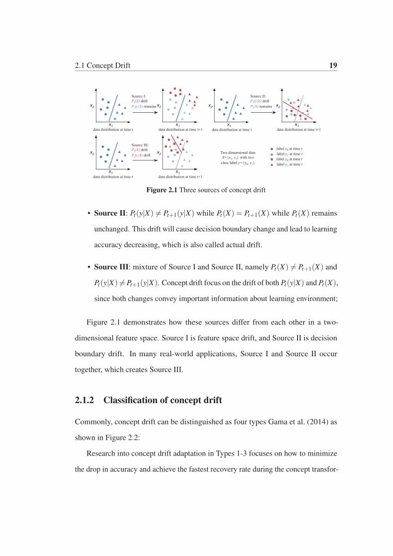
• Source I: Pt(X) �= Pt+1(X) while Pt(y|X) = Pt+1(y|X), that is, the research
focus is the drift in Pt(X) while Pt(y|X) remains unchanged. Since Pt(X) drift
does not affect the decision boundary, it has also been considered as virtual
drift Ramírez-Gallego et al. (2017).
2.1 Concept Drift 19
Source III:Pt(X) driftPt(y|X) drift
data distribution at time t data distribution at time t+1x1
x2
x1
x2
Source II:Pt(y|X) driftPt(X) remains
data distribution at time t data distribution at time t+1x1
x2
x1
x2
Source I:Pt(X) driftPt(y|X) remains
data distribution at time t data distribution at time t+1x1
x2
x1
x2
Two dimensional data X={x1, x2} with two class label y={y0, y1}
label y0 at time tlabel y1 at time tlabel y0 at time tlabel y1 at time t
Figure 2.1 Three sources of concept drift
• Source II: Pt(y|X) �= Pt+1(y|X) while Pt(X) = Pt+1(X) while Pt(X) remains
unchanged. This drift will cause decision boundary change and lead to learning
accuracy decreasing, which is also called actual drift.
• Source III: mixture of Source I and Source II, namely Pt(X) �= Pt+1(X) and
Pt(y|X) �=Pt+1(y|X). Concept drift focus on the drift of both Pt(y|X) and Pt(X),
since both changes convey important information about learning environment;
Figure 2.1 demonstrates how these sources differ from each other in a two-
dimensional feature space. Source I is feature space drift, and Source II is decision
boundary drift. In many real-world applications, Source I and Source II occur
together, which creates Source III.
2.1.2 Classification of concept drift
Commonly, concept drift can be distinguished as four types Gama et al. (2014) as
shown in Figure 2.2:
Research into concept drift adaptation in Types 1-3 focuses on how to minimize
the drop in accuracy and achieve the fastest recovery rate during the concept transfor-

20 Literature Review
SuddenDrift:A new concept occurs within a short time.s within a short time
Data
distribution
Time
GradualDrift:A new concept gradually replaces an old one over a period of time.ll l ld i d f ti
Data
distribution
Time
IncrementalDrift:The old concept incrementally changes to new concept over a period of time.ementally changes to new concept over a period of time
Data
distribution
Time
ReoccurringConcepts:The old concepts may reoccur after some time.ft ti
Data
distribution
Time
Figure 2.2 A demonstration of concept drift types
mation process. In contrast, the study of Type 4 drift emphasizes the use of historical
concepts, that is, how to find the best matched historical concepts with the shortest
time. The new concept may suddenly reoccur, incrementally reoccur, or gradually
reoccur.
To better demonstrate the differences between these types, the term “intermediate
concept” was introduced by Gama et al. (2014) to describe the transformation
between concepts. As mentioned by Liu et al. (2017a), a concept drift may not only
take place at an exact timestamp, but may also last for a long period. As a result,
intermediate concepts may appear during the transformation as one concept (starting
concept) changes to another (ending concept). An intermediate concept can be a
mixture of the starting concept and the ending concept, like the incremental drift, or
one of the starting or ending concept, such as the gradual drift.

2.1 Concept Drift 21
2.1.3 Related research topics and applications
Handling concept drift is not a standalone research subject but has a large number of
indirect usage scenarios. This section adopts this new perspective to review recent
developments in other research areas that benefit from handling the concept drift
problem.
2.1.3.1 Related research topics
i) Class imbalance. Class imbalance is a common problem in streaming data learning
in addition to concept drift Wang et al. (2013, 2018). Research effort has been made
to develop effective learning algorithms to tackle both problems at the same time. In
Ditzler and Polikar (2013), the authors presented two ensemble methods for learning
under concept drift with imbalanced class. The first method, Learn++ for Concept
Drift with SMOTE (Learn++.CDS), is extended from Learn++ for Non-Stationary
Environment (Learn++.NSE) Elwell and Polikar (2011) and combined with the
Synthetic Minority class Oversampling TEchnique (SMOTE). The second algo-
rithm, Learn++ for Non-stationary and Imbalanced Environments (Learn++.NIE),
improves on the previous method by employing a different penalty constraint to
prevent prediction accuracy bias and replacing SMOTE with bagging to avoid
oversampling. Ensemble of Subset Online Sequential Extreme Learning Machine
(ESOS-ELM) Mirza et al. (2015) is another ensemble method which uses Online
Sequential Extreme Learning Machine (OS-ELM) as a basic classifier to improve
performance with class imbalanced data. A concept drift detector is integrated to
retrain the classifier when drift occurs. The author then developed another algorithm
Mirza and Lin (2016), which is able to tackle multi-class imbalanced data with

22 Literature Review
concept drift. Wang et al. (2015) proposed two learning algorithms Oversampling-
based Online Bagging (OOB) and Undersampling-based Online Bagging (UOB),
which build an ensemble model to overcome the class imbalance in real time through
resampling and time-decayed metrics. Arabmakki and Kantardzic (2017) developed
an ensemble method which handles concept drift and class imbalance with additional
true label data limitation.
ii) Big data mining. Data mining in big data environments faces similar chal-
lenges to stream data mining Katal et al. (2013): data is generated at a fast rate
(Velocity) and distribution uncertainty always exists in the data (Variety), which
means that handling concept drift is crucial in big data applications. Additionally,
scalability is an important consideration because in big data environments, a data
stream may come in very large and potentially unpredictable quantities (Volume) and
cannot be processed in a single computer server. An attempt to handle concept drift
in a distributed computing environment was made by Andrzejak and Gomes (2012)
in which an Online Map-Reduce Drift Detection Method (OMR-DDM) was pro-
posed, using the combined online error rate of the parallel classification algorithms
to identify the changes in a big data stream. A recent study Tennant et al. (2017) pro-
posed another scalable stream data mining algorithm, called Micro-Cluster Nearest
Neighbor (MC-NN), based on nearest neighbor classifier. This method extends the
original micro-cluster algorithm Aggarwal et al. (2003) to adapt to concept drift by
monitoring classification error. This micro-cluster algorithm was further extended to
a parallel version using the map-reduce technique in Song et al. (2016) and applied
to solve the label-drift classification problem where class labels are not known in
advance Nguyen et al. (2016). Similar strategy has been applied in Liu et al. (2016a)
to develop an online competence-based concept drift detection algorithm.
2.1 Concept Drift 23
iii) Active learning and semi-supervised learning. Active learning is based on
the assumption that there is a large amount of unlabeled data but only a fraction
of them can be labeled by human effort. This is a common situation in stream
data applications, which are often also subject to the concept drift problem. In
Žliobaite et al. (2014), the authors presented a general framework that combines
active learning and concept drift adaptation. It first compares different instance-
sampling strategies for labeling to guarantee that the labeling cost will be under
budget, and that distribution bias will be prevented. A drift adaptation mechanism is
then adopted, based on the Drift Detection Method (DDM) Gama et al. (2004). In
Chu et al. (2011), the authors proposed a new active learning algorithm that primarily
aims to avoid bias in the sampling process of choosing instances for labeling. They
also introduced a memory loss factor to the model, enabling it to adapt to concept
drift.
Semi-supervised learning concerns how to use limited true label data more
efficiently by leveraging unsupervised techniques. In this scenario, additional design
effort is required to handle concept drift. For example, in Ditzler and Polikar
(2011), the authors applied a Gaussian Mixture model to both labeled and unlabeled
data, and assigned labels, which has the ability to adapt to gradual drift. Similarly,
Hosseini et al. (2015); Wu et al. (2012); Zhang et al. (2010) are all cluster-based
semi-supervised ensemble methods that aim to adapt to drift with limited true label
data. The latter are also able to recognize recurring concepts. In Chandra et al.
(2016), the author adopted a new perspective on the true label scarcity problem
by considering the true labeled data and unlabeled data as two independent non-
stationary data generating processes. Concept drift is handled asynchronously on
these two streams. The Semi-supervised Adaptive Novel class Detection (SAND)

24 Literature Review
algorithm Haque et al. (2016a,b) is another semi-supervised adaptive method which
detects concept drift on cluster boundaries.
iv) Decision Rules. Data-driven decision support systems need to be able to
adapt to concept drift in order to make accurate decisions and decision rules is the
main technique for this purpose. Kosina and Gama (2015) proposed a decision
rule induction algorithm, Very Fast Decision Rules (VFDR), to effectively process
stream data. An extended version, adaptive VFDR, was developed to handle concept
drift by dynamically adding and removing decision rules according to their error
rate which is monitored by drift detector. Instead of inducing rules from decision
trees, Le et al. (2017) proposed another decision rule algorithm based on PRISM
Cendrowska (1987) to directly induce rules from data. This algorithm is also able
to adapt to drift by monitoring the performance of each rule on a sliding window
of latest data. Pratama et al. (2015) also developed an adaptive decision making
algorithm based on fuzzy rules. The algorithm includes a rule pruning procedure,
which removes obsolete rules to adapt to changes, and a rule recall procedure to
adapt to recurring concepts.
This section by no means attempts to cover every research field in which concept
drift handling is used. There are many other studies that also consider concept drift
as a dual problem. For example, Yeh and Wang (2013) is a dimension reduction
algorithm to separate classes based on Least Squares Linear Discovery Analysis
(LSLDA), which is then extended to adapt to drift; Feature Extraction for explicit
concept Drift Detection (FEDD) Cavalcante et al. (2016) considered the concept drift
problem in time series and developed an online explicit drift detection method by
monitoring time series features; and Pratama et al. (2016) developed an incremental
scaffolding classification algorithm for complex tasks that also involve concept drift.

2.1 Concept Drift 25
2.1.3.2 Related applications
Handling concept drift is important to real-world applications because streaming data
are ubiquitous. Examples include network traffic, telecommunications, and financial
transactions, to name just three. Data mining tasks in these systems will inevitably
encounter the concept drift problem. In some cases, the ability to handle concept
drift becomes the key factor in improving system performance. A comprehensive
review of concept drift industrial applications can be found in Žliobaite et al. (2016),
in which the authors list many industrial examples of different types of application,
including monitoring and control, information management, analytics and diagnos-
tics. In this section previous studies are summarized from two aspects drift detection
applications and drift adaptation applications, to provide a guide for concept drift
applications from an academic research perspective to real-life applications.
Concept drift detection applications fulfill the industrial requirement of diagnos-
ing significant changes in the internal and external environment of industry trends
or customer preferences: for example, using drift detection technology to diagnose
changes in user preferences on news Harel et al. (2014). Similar tasks include fraud
detection in finance, intrusion detection in computer security, mobile masquerade de-
tection in telecommunications, topic changes in information document organization,
and clinical studies in the biomedical area.
Concept drift adaptation applications concern the maintenance of a continu-
ously effective evaluation and prediction system for industry. These applications
sometimes also involve drift detection technologies for better accuracy. A real case
represented in Sousa et al. (2016) is the design of a credit risk assessment framework
for dynamic credit scoring. Other real-world drift adaptation applications can be

26 Literature Review
found in customer churn prediction in telecommunication, traffic management in
transportation, production and service monitoring, recommendations for customers,
and bankruptcy prediction in finance.
With the rapid development of technology, learning with streaming data are
becoming more highly dimensional with larger sizes and faster speed. The new
challenges presented by big data streams require more advanced concept drift appli-
cations. One concern is how to handle concept drift problems in the IoT Morales
et al. (2016), where the huge quantity of big data streams require deeper insight and
a better understanding of concept drift.
2.2 Concept Drift Detection and Adaptation
This section focuses on summarizing concept drift detection algorithms. A general
drift detection framework is introduced in Section 2.2.1.1. Then, Section 2.2.1.2
systematically reviews and categorizes drift detection algorithms according to their
implementation details for each component in the framework. At last, Section
2.2.1.3 lists the state-of-the-art drift detection algorithms with comparisons of their
implementation details.
2.2.1 Concept drift detection
Drift detection refers to the techniques and mechanisms that characterize and quantify
concept drift via identifying change points or change time intervals Basseville and
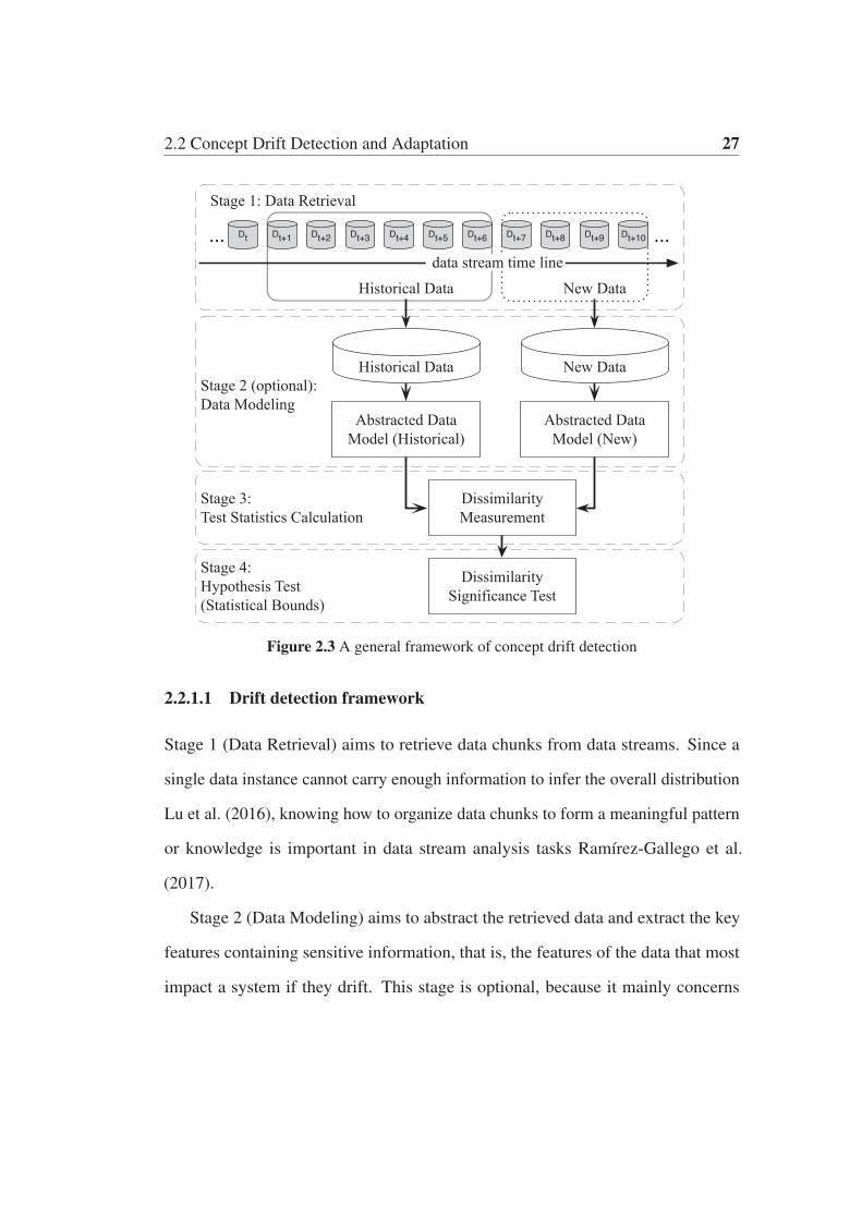
Nikiforov (1993). A general framework for drift detection contains four stages, as
shown in Figure 2.3.
2.2 Concept Drift Detection and Adaptation 27
Dt Dt+1 Dt+2 Dt+3 Dt+4 Dt+5 Dt+6 Dt+7 Dt+8 Dt+9 Dt+10
Historical Data New Data
Stage 1: Data Retrieval
data stream time line
Abstracted Data Model (New)
Abstracted DataModel (Historical)
Stage 2 (optional): Data Modeling
Historical Data New Data
Dissimilarity Measurement
Stage 3: Test Statistics Calculation
Dissimilarity Significance Test
Stage 4: Hypothesis Test (Statistical Bounds)
Figure 2.3 A general framework of concept drift detection
2.2.1.1 Drift detection framework
Stage 1 (Data Retrieval) aims to retrieve data chunks from data streams. Since a
single data instance cannot carry enough information to infer the overall distribution
Lu et al. (2016), knowing how to organize data chunks to form a meaningful pattern
or knowledge is important in data stream analysis tasks Ramírez-Gallego et al.
(2017).
Stage 2 (Data Modeling) aims to abstract the retrieved data and extract the key
features containing sensitive information, that is, the features of the data that most
impact a system if they drift. This stage is optional, because it mainly concerns

28 Literature Review
dimensionality reduction, or sample size reduction, to meet storage and online speed
requirements Liu et al. (2017a).
Stage 3 (Test Statistics Calculation) is the measurement of dissimilarity, or
distance estimation. It quantifies the severity of the drift and forms test statistics for
the hypothesis test. It is considered to be the most challenging aspect of concept
drift detection. The problem of how to define an accurate and robust dissimilarity
measurement is still an open question. A dissimilarity measurement can also be
used in clustering evaluation Silva et al. (2013), and to determine the dissimilarity
between sample sets Dries and Rückert (2009).
Stage 4 (Hypothesis Test) uses a specific hypothesis test to evaluate the sta-
tistical significance of the change observed in Stage 3, or the p-value. They are
used to determine drift detection accuracy by proving the statistical bounds of the
test statistics proposed in Stage 3. Without Stage 4, the test statistics acquired in
Stage 3 are meaningless for drift detection, because they cannot determine the drift
confidence interval, that is, how likely it is that the change is caused by concept drift
and not noise or random sample selection bias Lu et al. (2014). The most commonly
used hypothesis tests are: estimating the distribution of the test statistics Alippi
and Roveri (2008a); Gama et al. (2004), bootstrapping Bu et al. (2016); Dasu et al.
(2006), the permutation test Lu et al. (2014), and Hoeffding’s inequality-based bound
identification Frias-Blanco et al. (2015).
It is also worth to mention that, without Stage 1, the concept drift detection
problem can be considered as a two-sample test problem which examines whether
the population of two given sample sets are from the same distribution Dries and
Rückert (2009). In other words, any multivariate two-sample test is an option that can
be adopted in Stages 2-4 to detect concept drift Dries and Rückert (2009). However,

2.2 Concept Drift Detection and Adaptation 29
in some cases, the distribution drift may not be included in the target features,
therefore the selection of the target feature will affect the overall performance of
a learning system and is a critical problem in concept drift detection Yamada et al.
(2013).
2.2.1.2 Concept drift detection algorithms
A) Learner-based Dri f t Detection: Learner-based drift detection algorithms form
the largest category of algorithms. These algorithms focus on tracking changes
in the online error rate of base classifiers. If an increase or decrease of the error
rate is proven to be statistically significant, an upgrade process (drift alarm) will be
triggered.
One of the most-referenced concept drift detection algorithms is the DDM Gama
et al. (2004). It was the first algorithm to define the warning level and drift level for
concept drift detection. In this algorithm, Stage 1 is implemented by a landmark
time window, as shown in Figure 2.4. When a new data instance become available
for evaluation, DDM detects whether the overall online error rate within the time
window has increased significantly. If the confidence level of the observed error rate
change reaches the warning level, DDM starts to build a new learner while using the
old learner for predictions. If the change reached the drift level, the old learner will
be replaced by the new learner for further prediction tasks. To acquire the online error
rate, DDM needs a classifier to make the predictions. This process converts training
data to a learning model, which is considered as the Stage 2 (Data Modeling). The
test statistics in Stage 3 constitute the online error rate. The hypothesis test, Stage 4,
is conducted by estimating the distribution of the online error rate and calculating
the warning level and drift threshold.

30 Literature Review
t t+1 t+2 t+3 t+4 t+5 t+6 t+7 t+8 t+9 t+10
Historical DataNew Data
Figure 2.4 Landmark time window for drift detection. The starting point of the window is
fixed, while the end point of the window will be extended after a new data instance has been
received.
Similar implementations have been adopted and applied in the Learning with
Local Drift Detection (LLDD) Gama and Castillo (2006), Early Drift Detection
Method (EDDM) Baena-García et al. (2006), Heoffding’s inequality based Drift
Detection Method (HDDM) Frias-Blanco et al. (2015), Fuzzy Windowing Drift
Detection Method (FW-DDM) Liu et al. (2017b), Dynamic Extreme Learning
Machine (DELM) Xu and Wang (2017). LLDD modifies Stages 3 and 4, dividing the
overall drift detection problem into a set of decision tree node-based drift detection
problems; EDDM improves Stage 3 of DDM using the distance between two correct
classifications to improve the sensitivity of drift detection; HDDM modifies Stage
4 using Hoeffding’s inequality to identify the critical region of a drift; FW-DDM
improves Stage 1 of DDM using a fuzzy time window instead of a conventional
time window to address the gradual drift problem; DELM does not change the
DDM detection algorithm but uses a novel base learner, which is a single hidden
layer feedback neural network called Extreme Learning Machine (ELM) Huang et al.
(2006) to improve the adaptation process after a drift has been confirmed. EWMA for
Concept Drift Detection (ECDD) Ross et al. (2012) takes advantage of the error rate
to detect concept drift. ECDD employs the Exponentially Weighted Moving Average
(EWMA) chart to track changes in the error rate. The implementation of Stages 1-3
of ECDD is the same as for DDM, while Stage 4 is different. ECDD modifies the

2.2 Concept Drift Detection and Adaptation 31
t t+1 t+2 t+3 t+4 t+5 t+6 t+7 t+8 t+9 t+10
New DataHistorical Data
Figure 2.5 Two time windows for concept drift detection. The New Data window has to be
defined by the user.
conventional EWMA chart using a dynamic mean p0,t instead of the conventional
static mean p0, where p0,t is the estimated online error rate within time [0, t], and p0
implies the theoretical error rate when the learner was initially built. Accordingly,
the dynamic variance can be calculated by σ2Zt= p0,t(1− p0,t)
√λ
2−λ (1− (1−λ )2t)
where λ controls how much weight is given to more recent data as opposed to older
data, and λ = 0.2 is recommended by the authors. Also, when the test statistic of
the conventional EWMA chart is Zt > p0,t +0.5LσZt , ECDD will report a concept
drift warning; when Zt > p0,t +LσZt , ECDD will report a concept drift. The control
limits L is given by the authors through experimental evaluation.
In contrast to DDM and other similar algorithms, Statistical Test of Equal
Proportions Detection (STEPD) Nishida and Yamauchi (2007) detects error rate
change by comparing the most recent time window with the overall time window,
and for each timestamp, there are two time windows in the system, as shown in
Figure 2.5. The size of the new window must be defined by the user. According to
Nishida and Yamauchi (2007), the test statistic θSTEPD conforms to standard normal
distribution, denoted as θSTEPD ∼ N(0,1). The significance level of the warning
level and the drift level were suggested as αw = 0.05 and αd = 0.003 respectively.
As a result, the warning threshold and drift threshold can be easily calculated.

32 Literature Review
Another popular two-time window-based drift detection algorithm is ADaptive
WINdowing (ADWIN) Bifet and Gavaldà (2007). Unlike STEPD, ADWIN does not
require users to define the size of the compared windows in advance; it only needs
to specify the total size n of a "sufficiently large" window W . It then examines all
possible cuts of W and computes optimal sub-window sizes nhist and nnew according
to the rate of change between the two sub-windows whist and wnew. The test statistic
is the difference of the two sample means θADWIN = |μhist − μnew|. An optimal
cut is found when the difference exceeds a threshold with a predefined confidence
interval δ . The author proved that both the false positive rate and false negative
rate are bounded by δ . It is worth noting that many concept drift adaptation meth-
ods/algorithms in the literature are derived from or combined with ADWIN, such as
Bifet and Gavaldà (2009); Bifet et al. (2009a,b); Gomes et al. (2017b). Since their
drift detection methods are implemented with almost the same strategy, details will
be discussed further.
B) Distribution-based Dri f t Detection: The second largest category of drift
detection algorithms is data distribution-based drift detection. Algorithms of this
category use a distance function/metric to quantify the dissimilarity between the
distribution of historical data and the new data. If the dissimilarity is proven to be
statistically significantly different, the system will trigger a learning model upgrada-
tion process. These algorithms address concept drift from the root sources, which
is the distribution drift. Not only can they accurately identify the time of drift, they
can also provide location information about the drift. However, these algorithms are
usually reported as incurring higher computational cost than the learner-based drift
detection algorithms mentioned before Lu et al. (2016). In addition, these algorithms
usually require users to predefine the historical time window and new data window.

2.2 Concept Drift Detection and Adaptation 33
Two windows at timestamp: t+6
t+11
Historical Data New Data
t+1 t+2 t+3 t+4 t+5 t+6 t+7 t+8 t+9 t+10 t+11
Historical Data New Data
Two windows at timestamp: t+7
Dt Dt+1 Dt+2 Dt+3 Dt+4 Dt+5 Dt+6 Dt+7 Dt+8 Dt+9 Dt+10
Dt Dt+1 Dt+2 Dt+3 Dt+4 Dt+5 Dt+6 Dt+7 Dt+8 Dt+9 Dt+10
Figure 2.6 Two sliding time windows, of fixed size. The Historical Data window will be
fixed while the New Data window will keep moving.
The commonly used strategy is two sliding windows with the historical time window
fixed while sliding the new data window Dasu et al. (2006); Lu et al. (2014); Shao
et al. (2014), as shown in Figure 2.6.
According to the literature, the first formal treatment of change detection in data
streams was proposed by Kifer et al. (2004). In their study, the authors point out that
the most natural notion of distance between distributions is total variation, as defined
by: TV (P1,P2) = 2supE∈ε |P1(E)−P2(E)| or equivalently, when the distribution has
the density functions f1 and f2, distL1 =∫ | f1(x)− f2(x)|dx. This provides practical
guidance on the design of a distance function for distribution discrepancy analysis.
Accordingly, Kifer et al. (2004) proposed a family of distances, called Relativized
Discrepancy (RD). The authors also present the significance level of the distance
according to the number of data instances. The bounds on the probabilities of missed
detections and false alarms are theoretically proven, using Chernoff bounds and the
Vapnik-Chervonenkis dimension. The authors of Kifer et al. (2004) do not propose
novel high-dimensional friendly data models for Stage 2 (data modeling); instead,
they stress that a suitable model choice is an open question.

34 Literature Review
Another typical density-based drift detection algorithm is the information-theoretic
approach Dasu et al. (2006). The intuitive idea underlying this algorithm is to use
kdqTree to partition the historical and new data (multi-dimensional) into a set of bins,
denoted as A ,and then use Kullback-Leibler divergence to quantify the difference of
the density θITA in each bin. The hypothesis test applied by the information-theoretic
approach is bootstrapping that merging Whist, Wnew as Wall and resampling as W ′hist,
W ′new to recompute the θ ∗
ITA. Once the estimated probability P(θ ∗ITA ≥ θITA)< 1−α ,
concept drift is confirmed, where α is the significant level controlling the sensitivity
of drift detection.
Similar distribution-based drift detection methods/algorithms are: statistical
change detection for multi-dimensional data Song et al. (2007), Competence Model-
based drift detection (CM) Lu et al. (2016), a prototype-based classification model
for evolving data streams called SyncStream Shao et al. (2014), Equal Density
Estimation (EDE) Gu et al. (2016), Least Squares Density Difference-based Change
Detection Test (LSDD-CDT) Bu et al. (2016), an incremental version of LSDD-CDT
(LSDD-INC) Bu et al. (2017) and LDD-DSDA Liu et al. (2017a).
C) Multiple Hypothesis Test Dri f t Detection: Multiple hypothesis test drift
detection algorithms apply similar techniques to those mentioned in the previous two
categories. The novelty of these algorithms is that they use multiple hypothesis tests
to detect concept drift in different ways. These algorithms can be divided into two
groups: 1) parallel multiple hypothesis tests; and 2) hierarchical multiple hypothesis
tests.
The idea of parallel multiple hypothesis drift detection algorithm is demonstrated
in Figure 2.7. According to the literature, Just-In-Time adaptive classifiers Just-In-
Time adaptive classifiers (JIT) Alippi and Roveri (2008a) is the first algorithm that set
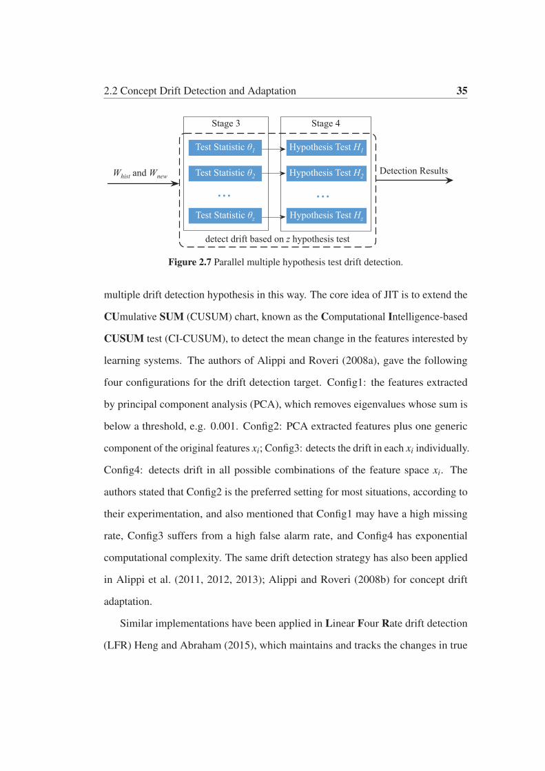
2.2 Concept Drift Detection and Adaptation 35
Test Statistic 1 Hypothesis Test H1
Test Statistic 2 Hypothesis Test H2
Test Statistic z Hypothesis Test Hz
... ...
Stage 3 Stage 4
Detection ResultsWhist and Wnew
detect drift based on z hypothesis test
Figure 2.7 Parallel multiple hypothesis test drift detection.
multiple drift detection hypothesis in this way. The core idea of JIT is to extend the
CUmulative SUM (CUSUM) chart, known as the Computational Intelligence-based
CUSUM test (CI-CUSUM), to detect the mean change in the features interested by
learning systems. The authors of Alippi and Roveri (2008a), gave the following
four configurations for the drift detection target. Config1: the features extracted
by principal component analysis (PCA), which removes eigenvalues whose sum is
below a threshold, e.g. 0.001. Config2: PCA extracted features plus one generic
component of the original features xi; Config3: detects the drift in each xi individually.
Config4: detects drift in all possible combinations of the feature space xi. The
authors stated that Config2 is the preferred setting for most situations, according to
their experimentation, and also mentioned that Config1 may have a high missing
rate, Config3 suffers from a high false alarm rate, and Config4 has exponential
computational complexity. The same drift detection strategy has also been applied
in Alippi et al. (2011, 2012, 2013); Alippi and Roveri (2008b) for concept drift
adaptation.
Similar implementations have been applied in Linear Four Rate drift detection
(LFR) Heng and Abraham (2015), which maintains and tracks the changes in true

36 Literature Review
Detection Layer: Standard Drift Detection Algorithms that have low drift
delay rate and low computational cost
Validation Layer: Depend on the detection layer
Stage 3 Stage 4
Detection ResultsWhist and Wnew Test Statistic detect Hypothesis Test Hdetect
Test Statistic valid Hypothesis Test Hvalid
Figure 2.8 Hierarchical multiple hypothesis test drift detection.
positive (TP), true negative (TN), false positive (FP) and false negative (FN) in an
online manner. The drift detection process also includes warning and drift levels.
Another parallel multiple hypothesis drift detection algorithm is three-layer
drift detection, based on Information Value and Jaccard similarity (IV-Jac) Zhang
et al. (2017). IV-Jac aims to individually address the label drift Pt(y) Layer I,
feature space drift Pt(X) Layer II, and decision boundary drift Pt(y|X) Layer III.
It extracts the Weight of Evidence (WoE) and Information Value (IV) from the
available data and then detects whether a significant change exists between the
WoE and IV extracted from Whist and Wnew by measuring the contribution to the
label for a feature value. The hypothesis test thresholds are predefined parameters
θPt(y) = θPt(X) = θPt(X |y) = 0.5 by default, which are chosen empirically.
Hierarchical drift detection is an emerging drift detection category that has
a multiple verification schema. The algorithms in this category usually detect
drift using an existing method, called the detection layer, and then apply an extra
hypothesis test, called the validation layer, to obtain a second validation of the
detected drift in a hierarchical way. The overall workflow is shown in Figure 2.8.

2.2 Concept Drift Detection and Adaptation 37
According to the claim made by Alippi et al. (2017), Hierarchical Change-
Detection Tests (HCDTs) is the first attempt to address concept drift using a hierar-
chical architecture. The detection layer can be any existing drift detection method
that has a low drift delay rate and low computational burden. The validation layer
will be activated and deactivated based on the results returned by the detection layer.
The authors recommend two strategies for designing the validation layer: 1) estimat-
ing the distribution of the test statistics by maximizing the likelihood; 2) adapting an
existing hypothesis test, such as the Kolmogorov-Smirnov test or the Cramer-Von
Mises test.
Hierarchical Linear-Four Rate (HLFR) Yu and Abraham (2017) is another re-
cently proposed hierarchical drift detection algorithm. It applies the drift detection
algorithm LFR as the detection layer. Once a drift is confirmed by the detection
layer, the validation layer will be triggered. The validation layer of HLFR is simply
a zero-one loss, denoted as E, over the ordered train-test split. If the estimated
zero-one loss exceeds a predefined threshold, η = 0.01, the validation layer will
confirm the drift and report to the learning system to trigger a model upgradation
process.
Two-Stage Multivariate Shift-Detection based on EWMA (TSMSD-EWMA)
Raza et al. (2015) has a very similar implementation, however, the authors do not
claim that their method is a hierarchy-based algorithm.
2.2.1.3 A summary of drift detection algorithms
Table 2.1 lists the most popular concept drift detection methods/algorithms based on
the general framework summarized in Section 2.2.1.1 (Figure 2.3).

38L
iter
ature
Rev
iew
Table 2.1 A summary of drift detection algorithms
Category Algorithms Stage 1 Stage 2 Stage 3 Stage 4
Learner-
basedDDM Landmark Learner Online error rate Distribution estimation
EDDM Landmark Learner Online error rate Distribution estimation
FW-DDM Landmark Learner Online error rate Distribution estimation
DELM Landmark Learner Online error rate Distribution estimation
STEPD Predefined whist, wnew Learner Error rate difference Distribution estimation
ADWIN Auto cut whist, wnew Learner Error rate difference Hoeffding’s Bound
ECDD Landmark Learner Online error rate EWMA Chart
HDDM Landmark Learner Online error rate Hoeffding’s Bound
LLDD Landmark, or sliding whist, wnew Decision trees Tree node error rate Hoeffding’s Bound
Data
distribution-
based
kdqTree Fixed whist, Sliding wnew kdqTree KL divergence Bootstrapping
CM Fixed whist, Sliding wnew Competence model Competence distance Permutation test
RD Fixed whist, Sliding wnew KS structure Relativized Discrepancy VC-Dimension
SCD Fixed whist, Sliding wnew kernel density estimator log-likelihood Distribution estimation
EDE Fixed whist, Sliding wnew Nearest neighbor Density scale Permutation test
SyncStream Fixed whist, Sliding wnew PCA P-Tree Wilcoxon test
LSDD-CDT Fixed whist, Sliding wnew Learner Relative difference Distribution estimation
LSDD-INC Fixed whist, Sliding wnew Learner Relative difference Distribution estimation
LDD-DSDA Fixed whist, Sliding wnew k-nearest neighbor Local drift degree. Distribution estimation
Multiple
Hypothesis
Tests
JIT Landmark Selected features 4 configurations Distribution estimation
LFR Landmark Learner TP, TN, FP, FN Distribution estimation
Three-layer Sliding both whist, wnew Learner P(y), P(X), P(X |y) Test statistic dist. estimation
TSMSD-EWMA Landmark Learner Online error rate EWMA Chart
HCDTs Landmark Depending on layers Depending on layers Depending on layer
HLFR Landmark Learner TP, TN, FP, FN Distribution estimation

2.2 Concept Drift Detection and Adaptation 39
2.2.2 Concept drift adaptation
This section focuses on strategies for updating existing learning models according
to the drift, which is known as drift adaptation or reaction. There are two main
categories of drift adaptation methods, namely single learning model adaptation and
ensemble learning for concept drift adaptation.
2.2.2.1 Single learning model adaptation
Single learning model adaptation strategy only activates one learning model for
classification/prediction tasks at each time point. The detailed implementation
methods can be further divided into three groups. i) select the most relevant data
instances to create new learning models to replace the obsolete one, which is also
called instance selection by Tsymbal (2004). Different weights may assign to the
seletected data instances according to the their arrive time or their competence with
regard to the current concept, or named as instance weighting by Tsymbal (2004);
ii) incrementally adjust the learning models’ parameters to adapt to current concept,
namely incremental learning.
i) Instance selection and weighting. In instance selection algorithms, the aim
is to select the instances relevant to the current concept Tsymbal (2004), and then
retraining a new model with the selected data to replace the obsolete model, which
has been considered as the most intuitive way of reacting to concept drift. An explicit
concept drift detector is required to decide when to retrain the model (see Section
2.2.1.2 for drift detection algorithms). A window strategy is often adopted in this
method to preserve the most recent for retraining. Paired Learners Bach and Maloof
(2008) follows this strategy and uses two learners: the stable learner and the reactive

40 Literature Review
learner. If the stable learner frequently misclassifies instances that the reactive
learner correctly classifies, a new concept is detected and the stable learner will be
replaced with the reactive learner. This method is simple to understand and easy to
implement, and can be applied at any point in the data stream. Similarly strategy
has been applied in Self Adjusting Memory kNN (SAMkNN) Losing et al. (2016),
which weights short term learner, long term learner based on their performance on
the most recent time frame. Instead of directly retraining the model, researchers have
also attempted to integrate the drift detection process with the retraining process
for specific machine learning algorithms. DELM Xu and Wang (2017) extends the
traditional ELM algorithm with the ability to handle concept drift by adaptively
adjusting the number of hidden layer nodes. When the classification error rate
increases, which could indicate the emergence of a concept drift, more nodes are
added to the network layers to improve its approximation capability. Similarly,
Forgetting Parameters Extreme Learning Machine (FP-ELM) Liu et al. (2016b) is
an ELM-extended method that adapts to drift by introducing a forgetting parameter
to the ELM model. A parallel version of ELM-based method Han et al. (2015) has
also been developed for high-speed classification tasks under concept drift. OS-ELM
Soares and Araújo (2016) is another online learning ensemble of repressor models
that integrates ELM using an ordered aggregation technique, which overcomes the
problem of defining the optimal ensemble size.
Instance-based lazy learners for handling concept drift have also been studied
intensively. The Just-in-Time adaptive classifier Alippi and Roveri (2008a,b) is such
a method which follows the "detect and update model" strategy. For drift detection,
it extends the traditional CUSUM test Manly and Mackenzie (2000) to a pdf-free
form. This detection method is then integrated with a k-Nearest Neighbor (kNN)

2.2 Concept Drift Detection and Adaptation 41
classifier Alippi and Roveri (2008b). When a concept drift is detected, old instances
(more than the last T samples) are removed from the case base. In later work, the
authors of Alippi et al. (2013); Silva et al. (2013) extended this algorithm to handle
recurrent concepts by computing and comparing current concept to previously stored
concepts. Noise-Enhanced Fast Context Switch (NEFCS) Lu et al. (2016) is another
kNN-based adaptive model. A competence model-based drift detection algorithm Lu
et al. (2014) was used to locate drift instances in the case base and distinguish them
from noise instances and a redundancy removal algorithm, Stepwise Redundancy
Removal (SRR), was developed to remove redundant instances in a uniform way,
guaranteeing that the reduced case base would still preserve enough information for
future drift detection.
ii) Incremental learning. An alternative to retraining an entire model is to
develop a model that incrementally and adaptively learns from the changing data.
Such models have the ability to partially update themselves when the underlying
data distribution changes. This approach is arguably more efficient than retraining
when the drift only occurs in local regions. Many methods in this category are based
on the decision tree algorithm because trees have the ability to examine and adapt to
each sub-region separately.
In a foundational work Domingos and Hulten (2000), an online decision tree
algorithm, called Very Fast Decision Tree (VFDT) was proposed, which is especially
tailored for high speed data streams. It uses Hoeffding bound to limit the number of
instances required for node splitting. This method has become very popular because
of its several distinct advantages: 1) it only needs to process each instance once
and does not store instances in memory or disk; 2) the tree itself only consumes a
small amount of space and does not grow with the number of instances it processes

42 Literature Review
unless there is new information in the data; 3) the cost of tree maintenance is very
low. An extended version, called CVFDT Hulten et al. (2001), was later proposed to
handle concept drift. In CVFDT, a sliding window is maintained to hold the latest
data. An alternative sub-tree is trained based on the window and its performance is
monitored. If the alternative sub-tree outperforms its original counterpart, it will be
used for future prediction and the original obsolete sub-tree will be pruned. VFDT
deal with continuous data (VFDTc) Gama et al. (2003) is another attempt to make
improvements to VFDT with several enhancements: the ability to handle numerical
attributes; the application of Naive Bayes classifiers in tree leaves and the ability
to detect and adapt to concept drift. Two node-level drift detection methods were
proposed based on monitoring differences between a node and its sub-nodes. The
first method uses classification error rate and the second directly checks distribution
difference. When a drift is detected on a node, the node becomes a leaf and its
descending sub-tree is removed. Later work Yang and Fong (2012, 2015) further
extended VFDTc using an adaptive leaf strategy that chooses the best classifier from
three options: majority voting, Naive Bayes and weighted Naive Bayes.
Despite the success of VFDT, recent studies Rutkowski et al. (2014, 2013) have
shown that its foundation, the Hoeffding bound, may not be appropriate for the node
splitting calculation because the variables it computes, the information gain, are not
independent. A new online decision tree model Rutkowski et al. (2015) was devel-
oped based on an alternative impurity measure. The paper shows that this measure
also reflects concept drift and can be used as a replacement measure in CVFDT. In
the same spirit, another decision tree algorithm Frías-Blanco et al. (2016) aims to
rectify the use of Hoeffding bound by computing the sum of independent random

2.2 Concept Drift Detection and Adaptation 43
variables, called relative frequencies. The error rate of sub-trees are monitored to
detect drift and are used for tree pruning.
2.2.2.2 Ensemble learning for concept drift adaptation
In contrast to single learning model adaptation, ensemble learning utilize multiple
models to make prediction/classification at each time point. The new learning
models can be created with explicit drift detection, that is, creating new models
for new detected concepts Bifet et al. (2010b); Gomes et al. (2017b), or be created
with predefined time frame Elwell and Polikar (2011), that is, creating new models
regularly for a fixed period.
Preserving and reusing old models can save significant effort to retrain a new
model for recurring concepts, and the old models may also be helpful to partial
current concept. This is the core idea of using ensemble methods to handle concept
drift. Ensemble methods have received much attention in stream data mining research
community in recent years. A survey about this research topic is Krawczyk et al.
(2017) Ensemble methods comprise a set of base classifiers that may have different
types or different parameters. The output of each base classifier is combined using
certain voting rules to predict the newly arrived data. Many adaptive ensemble
methods have been developed that aim to handle concept drift by extending classical
ensemble methods or by creating specific adaptive voting rules.
Bagging, Boosting and Random Forests are classical ensemble methods used
to improve the performance of single classifiers. They have all been extended for
handling streaming data with concept drift. An online version of the bagging method
was first proposed in Oza and Russell (2001) which uses each instance only once
to simulate the batch mode bagging. In a later study Bifet et al. (2010b), this

44 Literature Review
method was combined with the ADWIN drift detection algorithm Bifet and Gavaldà
(2007) to handle concept drift. When a concept drift is reported, the newly proposed
method, called LeVeraGing Bagging (LVGB), trains a new classifier on the latest
data to replace the existing classifier with the worst performance. Similarly, an
adaptive boosting method was developed in Chu and Zaniolo (2004) which handles
concept drift by monitoring prediction accuracy using a hypothesis test, assuming
that classification errors on non-drifting data should follow Gaussian distribution. In
a recent work Gomes et al. (2017b), the Adaptive Random Fores (ARF) algorithm
was proposed, which extends the random forest tree algorithm with a concept drift
detection method, such as ADWIN Bifet and Gavaldà (2007), to decide when to
replace an obsolete tree with a new one. A similar work can be found in Li et al.
(2015), which uses Hoeffding bound to distinguish concept drift from noise within
decision trees.
Besides extending classical methods, many new ensemble methods have been
developed to handle concept drift using novel voting techniques. Dynamic Weighted
Majority (DWM) Kolter and Maloof (2007) is such an ensemble method that is
capable of adapting to drifts with a simple set of weighted voting rules. It manages
base classifiers according to the performance of both the individual classifiers and
the global ensemble. If the ensemble misclassifies an instance, DWM will train
a new base classifier and add it to ensemble. If a base classifier misclassifies an
instance, DWM reduces its weight by a factor. When the weight of a base classifier
drops below a user defined threshold, DWM removes it from the ensemble. The
drawback of this method is that the adding classifier process may be triggered too
frequently, introducing performance issues on some occasions, such as when gradual
drift occurs. A well-known ensemble method, Learn++.NSE Elwell and Polikar

2.2 Concept Drift Detection and Adaptation 45
(2011), mitigates this issue by weighting base classifiers according to their prediction
error rate on the latest batch of data. If the error rate of the youngest classifier
exceeds 50%, a new classifier will be trained based on the latest data. This method
has several other benefits: it can easily adopt almost any base classifier algorithm; it
does not store history data, only the latest batch of data, which it only uses once to
train a new classifier; and it can handle sudden drift, gradual drift, and recurrent drift
because underperforming classifiers can be reactivated or deactivated as needed by
adjusting their weights. Other voting strategies than standard weighted voting have
also been applied to handle concept drift. Examples include hierarchical ensemble
structure Yin et al. (2015); Zhang et al. (2011), short term and long term memory
Losing et al. (2016); Xu et al. (2017) and dynamic ensemble sizes Pietruczuk et al.
(2016); You and Lin (2016).
A number of research efforts have been made that focus on developing ensemble
methods for handling concept drift of certain types. Accuracy Update Ensemble
(AUE) Brzezinski and Stefanowski (2011, 2014) was proposed with an emphasis
on handling both sudden drift and gradual drift equally well. It is a batch mode
weighted voting ensemble method based on incremental base classifiers. By doing
re-weighting, the ensemble is able react quickly to sudden drift. All classifiers are
also incrementally trained with the latest data, which ensures that the ensemble
evolves with gradual drift. The Optimal Weights Adjustment (OWA) method Zhang
et al. (2008) achieves the same goal by building ensembles using both weighted
instances and weighted classifiers for different concept drift types. The authors of
Sun et al. (2016) considered a special case of concept drift — class evolution —
the phenomenon of class emergence and disappearance. Recurring concepts are
handled in Gama and Kosina (2013); Gomes et al. (2014), which monitor concept

46 Literature Review
information to decide when to reactivate previously stored obsolete models. Ahmadi
and Kramer (2017) is another method that handles recurring concepts by refining the
concept pool to avoid redundancy.

Chapter 3
The Nature of Regional Drift
3.1 Introduction
In the literature, concept drift has been defined in many forms. The most referenced
definitions are A) ∃t : Ft(X ,y) �= Ft+1(X ,y) Lu et al. (2014), where Ft(X ,y) is a
function used to describe the distribution of the data received at time t, this function
can be a probability density function (PDF) or a cumulative distribution function
(CDF); and B) ∃t,X : Pt(X ,y) �= Pt+1(X ,y) Gama et al. (2014), where Pt(X ,y) is the
joint probability of X and y at time t. The definition A) only focus on time related
drift, the research scope of the drift detection based on this definition is almost the
same as two-sample test, where the "two samples" are the data received at t and
t +1. This definition contains no location information and is difficult to be compared
directly. In contrast, the definition B) has location information for discrete feature
space. However, it is invalid in continuous feature space. Besides these issues,
another critical problem is that neither definition A) nor B) can describe the types
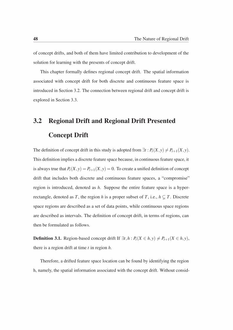
48 The Nature of Regional Drift
of concept drifts, and both of them have limited contribution to development of the
solution for learning with the presents of concept drift.
This chapter formally defines regional concept drift. The spatial information
associated with concept drift for both discrete and continuous feature space is
introduced in Section 3.2. The connection between regional drift and concept drift is
explored in Section 3.3.
3.2 Regional Drift and Regional Drift Presented
Concept Drift
The definition of concept drift in this study is adopted from ∃t : Pt(X ,y) �= Pt+1(X ,y).
This definition implies a discrete feature space because, in continuous feature space, it
is always true that Pt(X ,y) = Pt+1(X ,y) = 0. To create a unified definition of concept
drift that includes both discrete and continuous feature spaces, a “compromise”
region is introduced, denoted as h. Suppose the entire feature space is a hyper-
rectangle, denoted as T , the region h is a proper subset of T , i.e., h � T . Discrete
space regions are described as a set of data points, while continuous space regions
are described as intervals. The definition of concept drift, in terms of regions, can
then be formulated as follows.
Definition 3.1. Region-based concept drift If ∃t,h : Pt(X ∈ h,y) �= Pt+1(X ∈ h,y),
there is a region drift at time t in region h.
Therefore, a drifted feature space location can be found by identifying the region
h, namely, the spatial information associated with the concept drift. Without consid-

3.3 The Relationship between Regional Drift and Concept Drift 49
ering spatial information, updating a learning model may result in an unnecessary
reduction of training data and a delayed response to incremental drift.
3.3 The Relationship between Regional Drift
and Concept Drift
Given Definition 3.1, concept drift detection and adaptation could be converted into
regional drift detection and adaptation by breaking the concept drift problem down
into a set of regional drift problems. The intuition behind this idea is to divide a
big problem into a set of subproblems that can be conquered more easily if tackled
individually. The relationship between regional drift and concept drift is formally
described by the theorems that follow.
Theorem 3.1. If ∃t,h : Pt(X ∈ h,y) �= Pt+1(X ∈ h,y), then ∃Xi ∈ h : Pt(Xi,y) �=Pt+1(Xi,y) which represents concept drift in a discrete feature space, and ∃ΔXi ∈h : Pt(ΔXi,y) �= Pt+1(ΔXi,y) which represents drifts in a continuous feature space,
where ΔXi = {X : ‖X −Xi‖< ε,X ∈ h,ε > 0}.
Proof. In a discrete feature space, the region h is a set of data instances. According
to the probability mass function (PMF), Pt(X ∈ h,y) is equal to ΣXi∈hPt(Xi,y). In
shortened form, this is denoted as Σi∈h pit . If ph
t �= pht+1, i.e., ph
t − pht+1 �= 0, then
Σi∈h(pit − pi
t+1) �= 0. Therefore, there must be at least one point pit where pi
t − pit+1 �=
0, which means that pit �= pi
t+1 is true, namely ∃t,Xi ∈ h : Pt(Xi,y) �= Pt+1(Xi,y).
Similarly, we can prove that if ∃t,h : Pt(X ∈ h,y) �= Pt+1(X ∈ h,y), then ∃ΔXi ∈ h :
Pt(ΔXi,y) �= Pt+1(ΔXi,y).

50 The Nature of Regional Drift
Theorem 3.2. If ∀h∈H\T : Pt(X ∈ h,y) =Pt+1(X ∈ h,y), then Pt(X ,y) =Pt+1(X ,y)
indicate no drift in a discrete feature space, and Pt(ΔX ,y) = Pt+1(ΔX ,y) indicate no
drift in a continuous feature space, where H is the power set of the feature space T .
Proof. Given two regions in a discrete feature space where hi = h j ∪ {Xk}, if
Pt(X ∈ hi,y) = Pt+1(X ∈ hi,y) and Pt(X ∈ h j,y) = Pt+1(X ∈ h j,y), then Pt(X =
Xk,y)=Pt+1(X =Xk,y). Therefore, if ∀h∈H\T : Pt(X ∈ h,y)=Pt+1(X ∈ h,y), then
Pt(X ,y) = Pt+1(X ,y). Similarly, we can prove for the continuous feature space
Theorem 3.1 indicates that there must be a concept drift if a regional drift exists.
Therefore, concept drift detection can be simplified into a process that searches
for drifted regions. Theorem 3.2 shows that, if no regional drift exists, no concept
drift exists, which can be used as a guideline for concept drift adaptation, that is,
solving all regional drifts will also solve concept drift. These two theorems form the
foundation of our proposed concept drift adaptation algorithm.
Recall the two major types of concept drift: sudden drift and incremental drift.
Regional drift handles both well, as shown in Figure 3.1. Dividing the entire feature
space into a set of regions not only simplifies concept drift detection problems but
also reveals the spatial information associated with concept drift.
Now suppose, a one-dimensional feature space with two classes, c0 and c1,
suddenly drifts from the right side to the left side, or incrementally drifts from one
side to another. Existing drift detection algorithms focus on differences across the
entire feature domain. Hence, the system may not able to determine whether a change
is significant at the beginning of a slow incremental drift. By contrast, a small change
is significant to a region, and, as a result, regional drift will be discovered earlier.
Similarly, if the system addresses regional drifts individually, non-drifted regions

3.3
The
Relatio
nsh
ipbetw
eenR
egio
nal
Drift
and
Concep
tD
rift51
h0 h1 h2 h3 h4 h5 h6 h7 h8 h9
h0 h1 h2 h3 h4 h5 h6 h7 h8 h9
h0 h1 h2 h3 h4 h5 h6 h7 h8 h9
h0 h1 h2 h3 h4 h5 h6 h7 h8 h9
h0 h1 h2 h3 h4 h5 h6 h7 h8 h9
h0 h1 h2 h3 h4 h5 h6 h7 h8 h9
c0 c1
c0 c1
Decision Boundary at t
Decision Boundary at
t+1
drifted regions
Time: t+0
Time: t+1
Time: t+2
Time: t+3
Time: t+0
Time: t+1
h0 h1 h2 h3 h4 h5 h6 h7 h8 h9
h0 h1 h2 h3 h4 h5 h6 h7 h8 h9
c0 c1
c0 c1
Decision nBoundary at t
DDecision DBoundary atou
t+1
drifted regionsd if d i
Time: t+0
Time: t+1
(a) Sudden Drift
h0 h1 h2 h3 h4 h5 h6 h7 h8 h9
h0 h1 h2 h3 h4 h5 h6 h7 h8 h9
h0 h1 h2 h3 h4 h5 h6 h7 h8 h9
h0 h1 h2 h3 h4 h5 h6 h7 h8 h9
Time: t+0
Time: t+1
Time: t+2
Time: t+3
(b) Incremental Drift
not globally significant, but regionally significant
start triggering warning level
Figure 3.1 A demonstration of converting sudden drift and incremental drift to a set of regional drifts. Assume two 1D datasets consisting
of two classes c0, c1, one contains a sudden drift at t +1, as shown in (a), where the decision boundary suddenly changes. The other
dataset contains an incremental drift starting at t and ending at t +3, as shown in (b), where the decision boundary changes slightly
in each time step. The vector {h0, . . . ,h9} is a set of regions which constitute the entire feature space. Therefore, the sudden and the
incremental drifts can each be presented as a set of regional drifts. In (a), the drift is in region {h3, . . . ,h6}; in (b), the drift is in {h6}at time t + 1, or {h4, . . . ,h6} from t to t + 3. Without considering spatial information, for the adaptation of sudden drift in (a), data
d ∈ {h0,h1,h2,h7,h8,h9} will be wasted, and the training set will be shrunk unnecessarily. Similarly, the incremental drift in (b), i.e., the
drifts at t +1, t +2, will be ignored and drift detection will be delayed.

52 The Nature of Regional Drift
remain unchanged, such as the training data in region {h0,h1,h3} and {h7,h8,h9}.
This reduces the risk of unnecessarily shrinking the training data.
According to Theorem 3.1, any concept drift can be detected, regardless of type,
by detecting whether a region in the domain has incurred a statistically significant
change. Similarly, according to Theorem 3.2, a concept drift problem can be ad-
dressed by ensuring there is no significant change in any region of the domain. In
other words, concept drift adaptation problems can be converted into a set of regional
drift problems, and addressing regional drift problems guarantees that concept drift
problems will be solved simultaneously.
3.4 Summary
The main contribution of this chapter is a novel definition of concept drift, namely
regional drift, which is proposed to elaborate the how the data distribution changes
from both time and spatial perspective and to uniformly describe different types of
concept drift. This chapter also theoretically proved that addressing regional drift
will guarantee other types of drift solved simultaneously. The implementation details
of region h are discussed in Chapter 6.

Chapter 4
Concept Drift Detection via
Accumulating Regional Density
Discrepancies
4.1 Introduction
This section focuses on addressing the weaknesses in distribution-based drift detec-
tion algorithms. Since these algorithms directly address the root cause of concept
drift, which is a variation in the data distribution, and are capable of representing
corresponding confidence intervals, they have been reported as the most accurate
drift detection methods Dasu et al. (2006); Kifer et al. (2004); Lu et al. (2016); Shao
et al. (2014). Although this type of drift detection algorithm has made remarkable
achievements, they still face the following bottlenecks:
1) Regional drifts were not taken into consideration, and drift sensitivity was
increased at the cost of increasing false alarms. Existing algorithms detect drifts in

54 Concept Drift Detection via Accumulating Regional Density Discrepancies
terms of the entire sample set but do not consider any regional changes in sub-sample
sets. Consequently, the test statistics of regional drifts may eventually be diluted
by stable regions, which decreases sensitivity Haque et al. (2016b). Even if the
algorithms can successfully capture a distribution drift caused by regional density
inequality, they are not able to distinguish whether this drift is caused by a serious
regional drift or a moderate global drift;
2) Existing distribution-based drift detection methods lack tailored statistical
significance tests. For example, Dasu et al. (2006) used bootstrapping Efron and
Tibshirani (1994) for statistical analysis, and Shao et al. (2014) used the Wilcoxon
test. From their experiments, it can be seen that different significance tests result
in different performance outcomes. Statistical analysis is critical to drift detection
accuracy, and an adequate explanation is indispensable to justify the relationship
between significance tests and test statistics Kifer et al. (2004). Therefore, to improve
the sensitivity of drift detection and to propose a tailored significance test, this paper
proposes a novel concept drift detection algorithm called NN-DVI. NN-DVI requires
no prior knowledge of the data distribution. Instead, it estimates the dissimilarity
between datasets in terms of the instances’ neighbors. Compared to other distribution-
based drift detection algorithms, the proposed NN-DVI method demonstrates the
following advantages:
• It is robust to one-dimensional data, as well as high-dimensional data.
• It is sensitive to concept drift caused by regional density changes and is robust
to noise.
• The distribution of the proposed distance metric is proven theoretically which
provides a statistical bound to guarantee the number of false alarms.

4.2 Preliminary 55
• It can describe detected changes by highlighting suspicious regions, and has
been tested in real-world applications.
This chapter formally presents the proposed drift detection method, NN-DVI,
which consists of three parts. In Section 4.2, the preliminaries are introduced. Then
the first part, which is a data modeling approach that retrieves critical information
and presents datasets as an abstracted model, is explained in details in Section 4.3.
The second part, which is a distance metric that accumulates regional density changes
to quantify the overall discrepancy between data sets, is explained in Section 4.4.1.
The third part, which is a tailored statistical significant test for the distance metric,
is explained in Section 4.4.2. The properties of the distance metric are discussed,
and its distribution has been theoretically proved. Followed by Section 4.4.3 that
provides the implementation details of NN-DVI. Finally, Section 4.5 evaluates the
developed algorithms on both synthetic datasets and real-world applications.
4.2 Preliminary
An important element of this chapter is multiset theory Blizard (1988). In contrast
to classic set theory, multiset theory defines a multiset (or bag) as a collection of
elements in which duplicates of the elements are allowed. The multiplicity of an
element, denoted as m(x), is the number of the element x in a specific multiset.
The cardinality is the total number of elements in a multiset, including repeated
memberships. For example, in the multiset A = {a,a,b,c,c,c}, the multiplicities of
the members a, b and c are respectively 2, 1 and 3, and the cardinality of A is 6. A
multiset can be formally defined as:

56 Concept Drift Detection via Accumulating Regional Density Discrepancies
Definition 4.1. Blizard (1988)(Multiset) A multiset is defined as a 2-tuple (A, m)
where A is a set of elements and m : A → N≥1 is the multiplicity function from A to
the set N≥1 = {1,2,3, . . .}. Formally, a multiset is denoted as
M = {(a,m(a)) : a ∈ A,m : A → N≥1} (4.1)
The multiplicity operations involved in this chapter are listed below.
Definition 4.2. Blizard (1988)(Multiset Indicator Function) Indicator function
IA : X → N, is defined by
IA(x) =
⎧⎪⎪⎨⎪⎪⎩
m(x), if x ∈ A
0, if x /∈ A(4.2)
Definition 4.3. Blizard (1988)(Multiset Intersection) Intersection indicator func-
tion of multiset A and B on element x is
IA∩B(x) = min{IA(x),IB(x)} (4.3)
Definition 4.4. Blizard (1988)(Multiset Union) Union indicator function of multiset
A and B on element x is
IA∪B(x) = max{IA(x),IB(x)} (4.4)

4.3 Nearest Neighbor-based Data Embedding 57
Definition 4.5. Blizard (1988)(Multiset Di f f erence) The set difference indicator
function of multiset A to B on element x is
IA\B(x) = max{0,IA(x)− IB(x)} (4.5)
Definition 4.6. Blizard (1988)(Multiset Element Sum) The sum indicator function
of multiset A and B on element x is
IA�B(x) = IA(x)+ IB(x) (4.6)
Definition 4.7. Blizard (1988)(Multiset Cardinality) The cardinality of a multiset
A is the sum of the indicator function values
|A|= ∑x∈X
IA(x) (4.7)
where X is the set of unique element in A
These multiplicity functions provide the basic set of operators for our algorithm.
4.3 Nearest Neighbor-based Data Embedding
Data distribution-based concept drift detection has been reported as the most sensitive
and convincing detection method Lu et al. (2016, 2014) because it directly addresses
the root causes of concept drift and can represent the corresponding confidence
interval. According to the literature, a typical distribution-based detection method
consists of three components. The first component is a data representation model
through which critical information is retrieved and irrelevant details are discarded.

58 Concept Drift Detection via Accumulating Regional Density Discrepancies
Incoming Data
New Abstracted Data Model
Historical Abstracted Data Model
Dissimilarity Measurement
Dissimilarity Significant Test
Historical Data
1) Data Modelling
2) Distance Function:total variation
3) Statistical Significance Test:permutation test
Incoming Data
New Abstracted Data Model
Historical Abstracted Data Model
Dissimilarity Measurement
Dissimilarity Significant Test
Historical Data
1) Data Modelling
2) Distance Function:total variation
3) Statistical Significance Test:permutation test
Figure 4.1 A general framework for distribution-oriented concept drift detection
The second component is a specific dissimilarity function designed to measure the
discrepancies between the data models. One of the most natural notions for the
distance between distributions is the total variation, or the L1 norm Kawahara and
Sugiyama (2012). The third component is a statistical significance test. Statistical
significance, namely the p-value, is the probability of obtaining the least extreme
result given that a null hypothesis is true. In drift detection, the null hypothesis
is true when the detected discrepancies are not caused by concept drift. As a
non-parametric test, a permutation test is a good option for empirically estimating
statistical significance. An overall framework for distribution-oriented concept drift
detection is summarized in Figure 4.1.

4.3 Nearest Neighbor-based Data Embedding 59
4.3.1 Modelling data as a set of high-resolution partitions
Space partitioning is defined as the process of dividing a feature space into two or
more disjoint subsets. Any data instance in the feature space can then be identified
as residing in exactly one of the subsets. When dealing with discrete datasets, it
is often infeasible to directly estimate the similarity between data instances Dasu
et al. (2006). One of the most popular solutions is to accumulate the differences
of empirical probability density through the divided non-overlapping subsets Dasu
et al. (2006). For example, a histogram is one of the most popular ways to assess
the probability distribution of a given variable by depicting the frequencies of
observations occurring in certain ranges of values (bins), where the bins are the
disjoint subsets. In concept drift problems, if two sample sets are drawn from an
identical distribution, every partition should have a similar number of data points,
namely the empirical probability density (num o f data points in one partitiontotal num o f data points ) in each
partition will be similar. Otherwise, a statistical significant difference between their
empirical probability density will be found.
Currently, in related research, space partitioning methods directly contribute to
the accuracy of drift detection Lu et al. (2016). As shown in Figure 4.2, the similarity
between sample sets will always be zero if a partitioning schema cannot explicitly
map similar items into the same partitions, like the 8×8 partitioning schema in
Figure 4.2(c). As a result, the detected density change will be invalid. By the same
token, if a partitioning schema mistakenly maps non-similar items into the same
partitions, the dissimilarity between testing sample sets will always be zero. A drift
detection algorithm will lose its sensitivity to density drifts, especially when only a
few data instances are available for evaluating the partitioning schema. Optimizing
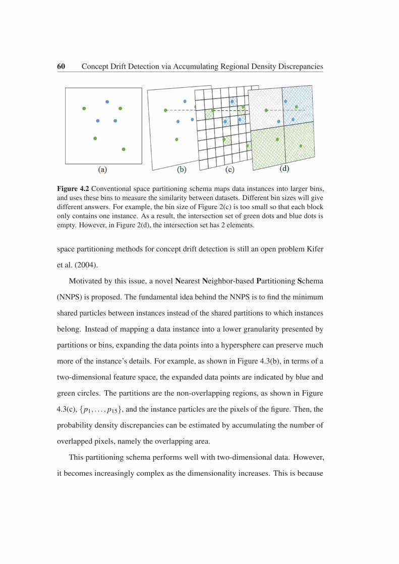
60 Concept Drift Detection via Accumulating Regional Density Discrepancies
Figure 4.2 Conventional space partitioning schema maps data instances into larger bins,
and uses these bins to measure the similarity between datasets. Different bin sizes will give
different answers. For example, the bin size of Figure 2(c) is too small so that each block
only contains one instance. As a result, the intersection set of green dots and blue dots is
empty. However, in Figure 2(d), the intersection set has 2 elements.
space partitioning methods for concept drift detection is still an open problem Kifer
et al. (2004).
Motivated by this issue, a novel Nearest Neighbor-based Partitioning Schema
(NNPS) is proposed. The fundamental idea behind the NNPS is to find the minimum
shared particles between instances instead of the shared partitions to which instances
belong. Instead of mapping a data instance into a lower granularity presented by
partitions or bins, expanding the data points into a hypersphere can preserve much
more of the instance’s details. For example, as shown in Figure 4.3(b), in terms of a
two-dimensional feature space, the expanded data points are indicated by blue and
green circles. The partitions are the non-overlapping regions, as shown in Figure
4.3(c), {p1, . . . , p15}, and the instance particles are the pixels of the figure. Then, the
probability density discrepancies can be estimated by accumulating the number of
overlapped pixels, namely the overlapping area.
This partitioning schema performs well with two-dimensional data. However,
it becomes increasingly complex as the dimensionality increases. This is because

4.3
Nearest
Neig
hbor-b
asedD
ataE
mbed
din
g61
(a) (c)(b)
p1
p2p3
p4
p5
p9
p15
p14
p6
p13
p12
p10
p7 p11p8
d1
d2
d3
d4
d5
d6
d7
d1
d2
d3
d4
d5
d6
d7
Figure 4.3 The proposed instance-oriented space partitioning schema aims to find the primary elements that consist of data instances, and
then use these elements to measure the similarity between datasets. In a 2d domain, let us consider each data instance as a circle rather
than a dot and the entire domain is a by n×n pixels square, as shown in Figure 3(b). Then the pixels are the primary elements which
constitute the data instances, and data instances can be represented by a set of pixels located in their circles. Therefore, the similarity
between instances can be simply estimated by counting the shared pixels located in the overlapping regions, such as the similarity
between d1 and d2 can be estimated by|p2|
|p1|+|p2|+|p3| , where |p1| indicates the number of pixels in region p1 as shown in Figure 3(c)

62 Concept Drift Detection via Accumulating Regional Density Discrepancies
Figure 4.4 Using a k-nearest neighbor data presenting model to replace the hyperspheres
model, the arrow in (b) indicates the relationship of k-nearest neighbors. For example,
d1 → d4 indicates that d4 is a kNN member of d1 while d1 is not a kNN member of d4. As
long as there is a connection between two data instances, they are considered as neighbors.
Then the datasets can be presented as a set of connections, as shown in (c). If each connection
is considered as one component of a data instance, namely a slice of a instance, then the data
instance d1 is a composite of one slice of itself, one slice from d2 and one slice from d4, as
shown in (d). Then, (e) illustrates the difference between conventional partitioning methods
and the NNPS
the intersecting regions between hyperspheres are difficult to explicitly calculate in
high dimensional space. Therefore, to further optimize the partitioning schema, a
k-nearest neighbor model to replace the hyperspheres model is applied.

4.3 Nearest Neighbor-based Data Embedding 63
An intuitive explanation for how a nearest neighbor model describes these in-
stance particles is that close located data instances have hidden connections, and
such connections can be used as the most basic element to constitute data instances.
As shown in Figure 4.4(d), unlike conventional partitioning schemas, which group
instances into different partitions, NNPS slices an instance into several particles, and
uses these particles to constitute instances. An overview of the difference between
the NNPS and conventional partitioning schemas is shown in Figure 4.4(e). To
overcome the bias caused by high granule mapping, NNPS extends instances into a
more detailed granule. This process is also called instance discretization or instance
quantization. Instead of measuring similarities in a conventional space partitioning
schema, applying shared instance particles can pass more instance details to the
sample sets, thereby making similarity measures more sensitive to small changes.
The concept of instance particles is formally defined as follows.
Definition 4.8. (Instance Particle) Given a di ∈ D, if the set Ki contains all neigh-
bors of di, then an instance particle based on di is defined as pdi = (di,Ki).
Example 4.1. Denote the data sample set as D = {d1,d2,d3,d4} and the neighbor
sets are K1 = {d1,d2}, K2 = {d1,d2,d3}, K3 = {d2,d3,d4}, K4 = {d3,d4}. Then
the instance particles are:
⎧⎪⎪⎪⎪⎪⎪⎪⎪⎪⎪⎨⎪⎪⎪⎪⎪⎪⎪⎪⎪⎪⎩
pd1= p(d1,K1) = (d1,{d1,d2})
pd2= p(d2,K2) = (d2,{d1,d2,d3})
pd3= p(d3,K3) = (d3,{d2,d3,d4})
pd4= p(d4,K4) = (d4,{d3,d4})
(4.8)

64 Concept Drift Detection via Accumulating Regional Density Discrepancies
The proposed NNPS breaks one data instance into a set of instance particles,
thereby transforming each discrete data instance into a set of shared instance particles.
As a result, the differences between data instances can be preserved for measuring
the distance between sample sets.
Definition 4.9. (Instance Particle Group) Given an instance dk ∈ D, the particle
group of dk is defined as P(dk) = {pdi : if dk ∈ Ki, i = 1,2, . . . , |D|}, where pdi =
(di,Ki).
Example 4.2. Referring to example 4.1, the data instances belonging to D repre-
sented by the instance particles are:
⎧⎪⎪⎪⎪⎪⎪⎪⎪⎪⎪⎨⎪⎪⎪⎪⎪⎪⎪⎪⎪⎪⎩
P(d1) = {pd1,pd2
}
P(d2) = {pd1,pd2
,pd3}
P(d3) = {pd2,pd3
,pd4}
P(d4) = {pd3,pd4
}
(4.9)
Definition 4.10. Given a sample set Sk ⊆ D, the particle group of Sk is defined as
P(Sk) = {⋃di∈SkP(di)}, where P(di) is the particle group of di.
Example 4.3. Referring to example 4.1, and given two sample sets S1 = {d1,d2},
S2 = {d3,d4}, then we have
⎧⎪⎪⎨⎪⎪⎩
P(S1) = P(d1)∪P(d2) = {pd1,pd2
,pd3}
P(S2) = P(d3)∪P(d4) = {pd2,pd3
,pd4}
(4.10)
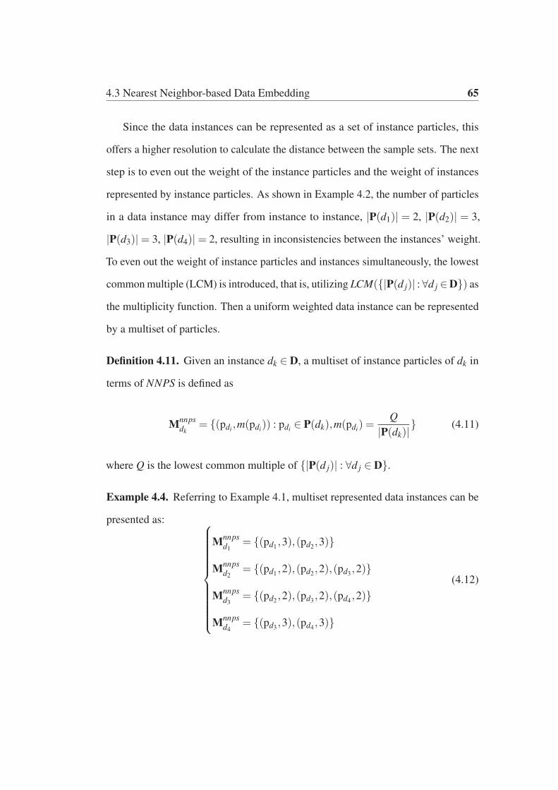
4.3 Nearest Neighbor-based Data Embedding 65
Since the data instances can be represented as a set of instance particles, this
offers a higher resolution to calculate the distance between the sample sets. The next
step is to even out the weight of the instance particles and the weight of instances
represented by instance particles. As shown in Example 4.2, the number of particles
in a data instance may differ from instance to instance, |P(d1)| = 2, |P(d2)| = 3,
|P(d3)|= 3, |P(d4)|= 2, resulting in inconsistencies between the instances’ weight.
To even out the weight of instance particles and instances simultaneously, the lowest
common multiple (LCM) is introduced, that is, utilizing LCM({|P(d j)| : ∀d j ∈D}) as
the multiplicity function. Then a uniform weighted data instance can be represented
by a multiset of particles.
Definition 4.11. Given an instance dk ∈ D, a multiset of instance particles of dk in
terms of NNPS is defined as
Mnnpsdk
= {(pdi ,m(pdi)) : pdi ∈ P(dk),m(pdi) =Q
|P(dk)|} (4.11)
where Q is the lowest common multiple of {|P(d j)| : ∀d j ∈ D}.
Example 4.4. Referring to Example 4.1, multiset represented data instances can be
presented as: ⎧⎪⎪⎪⎪⎪⎪⎪⎪⎪⎪⎨⎪⎪⎪⎪⎪⎪⎪⎪⎪⎪⎩
Mnnpsd1
= {(pd1,3),(pd2
,3)}
Mnnpsd2
= {(pd1,2),(pd2
,2),(pd3,2)}
Mnnpsd3
= {(pd2,2),(pd3
,2),(pd4,2)}
Mnnpsd4
= {(pd3,3),(pd4
,3)}
(4.12)
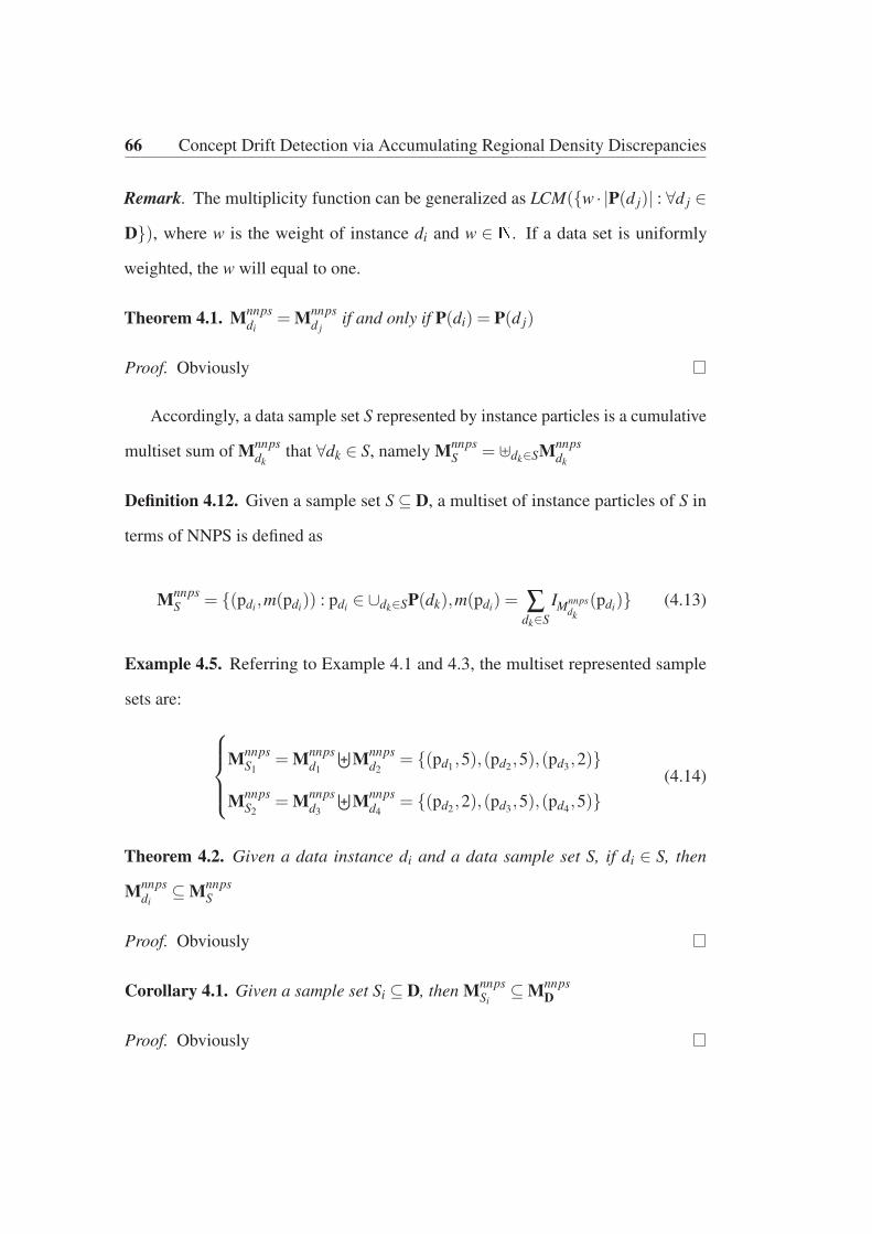
66 Concept Drift Detection via Accumulating Regional Density Discrepancies
Remark. The multiplicity function can be generalized as LCM({w · |P(d j)| : ∀d j ∈D}), where w is the weight of instance di and w ∈ �. If a data set is uniformly
weighted, the w will equal to one.
Theorem 4.1. Mnnpsdi
= Mnnpsd j
if and only if P(di) = P(d j)
Proof. Obviously
Accordingly, a data sample set S represented by instance particles is a cumulative
multiset sum of Mnnpsdk
that ∀dk ∈ S, namely MnnpsS = �dk∈SMnnps
dk
Definition 4.12. Given a sample set S ⊆ D, a multiset of instance particles of S in
terms of NNPS is defined as
MnnpsS = {(pdi ,m(pdi)) : pdi ∈ ∪dk∈SP(dk),m(pdi) = ∑
dk∈SIMnnps
dk(pdi)} (4.13)
Example 4.5. Referring to Example 4.1 and 4.3, the multiset represented sample
sets are:
⎧⎪⎪⎨⎪⎪⎩
MnnpsS1
= Mnnpsd1
⊎Mnnps
d2= {(pd1
,5),(pd2,5),(pd3
,2)}
MnnpsS2
= Mnnpsd3
⊎Mnnps
d4= {(pd2
,2),(pd3,5),(pd4
,5)}(4.14)
Theorem 4.2. Given a data instance di and a data sample set S, if di ∈ S, then
Mnnpsdi
⊆ MnnpsS
Proof. Obviously
Corollary 4.1. Given a sample set Si ⊆ D, then MnnpsSi
⊆ MnnpsD
Proof. Obviously

4.3 Nearest Neighbor-based Data Embedding 67
In summary, NNPS aims to extend instances into a lower granularity to provide a
more detailed shared subspace for measuring similarity and dissimilarity. In NNPS,
each data instance is a partition, and the hidden relationships between instances are
the primary elements that lie in the regions. Compared to conventional “bin”-based
partitioning methods, which only consider the similarity between data instances
as 1 (located in the same bin) or 0 (located in different bins), NNPS can preserve
the similarity between data instances, therefore becoming more sensitive to small
discrepancies. In addition, the datasets presented by NNPS are the accumulation
of instance particles from every partition. As a result, the density discrepancies in
partitions will also be accumulated and reflected in the similarity or dissimilarity
measurement.
4.3.2 Partition size optimization
The selection of the number of nearest neighbors (the k value of knn) is critical to
controlling the resolution and is the only parameter of the NNPS. To select the best
resolution to construct NNPS, a novel discretization controlling method is proposed,
called the instance particle independence coefficient, or simply independence, to
quantify the granule information contained at different granule levels.
In the context of the NNPS, the granule information indicator is defined as how
likely it is that a group of instance particles will appear together, namely the joint
probability of a group of instance particles occurring. Intuitively, in the proposed
data model, the primary element of a data set is the instance particles. The NNPS is
constructed based on these elements. If a group of such elements is always shown

68 Concept Drift Detection via Accumulating Regional Density Discrepancies
Figure 4.5 An example of grouped instance particles. Since p(d2) and p(d3) are always
grouped together, the difference between d2 and d3 is equal to zero. If such a group is large
enough, it will be impossible to identify whether there is a drift within them. Consequently,
the sensitiveness of NNPS on concept drift will decrease.
together, with a joint probability equal to 1, it would be impossible to detect drifts
inside this group, as shown in Figure 4.5.
In other words, the granule information indicator of the proposed data model
describes the average region size assumed to have no concept drift. From a practical
point of view, investigating the joint probability of every combination is neither
computationally-friendly nor storage efficient. Alternatively, such indicators can be
acquired through measuring the independence of every instance particle. The higher
the probability that an instance particle will appear in a certain instance particle
group, the less independence that instance particle has. To estimate the overall
independence of a given instance particle p(di), the indicator of its independence is
defined as the average value of the conditional probability of its connected instance
particles.

4.4 Nearest Neighbor-based Density Variation Identification 69
Definition 4.13. (Independence o f Instance Particle) The independence indicator
of a given instance particle is defined as
independence(pdi) = 1− 1
|P(di)| ∑pdk∈P(di)
p(pdk ,pdi) (4.15)
where p(pdk ,pdi) is the probability that pdk ∈ P(di) and pdi ∈ P(di)
Definition 4.14. (Independence o f NNPS) The independence of the NNPS is de-
fined as the average value of instance particles’ independence, denoted as:
independence =1
|D| ∑pdi∈
⋃dk∈D P(dk)
independence(pdi) (4.16)
With information granularity metrics, learning models can recognize and exploit
the meaningful pieces of knowledge present in data so that different features and
regularities can be revealed. This provides theoretical guidance for selecting the
k-value, which is maxk
{independence}.
4.4 Nearest Neighbor-based Density Variation Identi-
fication
4.4.1 A regional drift-oriented distance function
Since data instances and datasets are now presented by multisets, the distance
between them can be quantified by set-related metrics in terms of Definitions 4.1-
4.7. The metrics applied in this paper are the number of different instance particles
between two given multisets, denoted as dnnps.

70 Concept Drift Detection via Accumulating Regional Density Discrepancies
Definition 4.15. NNPS dissimilarity measurement Given two sample sets A,B ⊆ D,
the NNPS-based distance between them is calculated by accumulating the differences
in the number of instance particles, and it can be normalized by dividing the number
of unique instance particles, denoted as
dnnps(MnnpsA ,Mnnps
B )
=1
|P(A)∪P(B)| ∑pdi∈P(A)∪P(B)
|IMnnpsA
(pdi)− IMnnpsB
(pdi)|IMnnps
A(pdi)+ IMnnps
B(pdi)
(4.17)
Example 4.6. Referring to Example 4.5, the similarity is calculated as:
dnnps(MnnpsS1
,MnnpsS2
)
=1
|P(S1)∪P(S2)| ·( |IMnnps
S1
(pd1)− IMnnps
S2
(pd1)|
IMnnpsS1
(pd1)+ IMnnps
S2
(pd1)
+|IMnnps
S1
(pd2)− IMnnps
S2
(pd2)|
IMnnpsS1
(pd2)+ IMnnps
S2
(pd2)
+|IMnnps
S1
(pd3)− IMnnps
S2
(pd3)|
IMnnpsS1
(pd3)+ IMnnps
S2
(pd3)
+|IMnnps
S1
(pd4)− IMnnps
S2
(pd4)|
IMnnpsS1
(pd4)+ IMnnps
S2
(pd4)
)
=1
4(|5−0|
5+
|5−2|7
+|2−5|
7+
|0−5|5
)
=5
7≈ 0.71
(4.18)
similarly, if S1 = {d1,d3} and S2 = {d2,d4} we have
dnnps(MnnpsS1
,MnnpsS2
)≈ 0.31 (4.19)

4.4 Nearest Neighbor-based Density Variation Identification 71
else if S1 = {d1,d4} and S2 = {d2,d3} we have
dnnps(MnnpsS1
,MnnpsS2
)≈ 0.17 (4.20)
an illustration to demonstrate how dnnps reflects the density dissimilarity between
data sets is shown in Figure 4.6.
4.4.2 Statistical guarantee
Measuring the difference between two sample sets is only one aspect of detecting
concept drift. Another aspect is to provide adequate evidence to determine how likely
it is that there will be such a difference if the given sample sets are drawn from an
identical distribution. Null hypothesis testing, or the so-called p-value approach, is
widely used to address similar problems. In our case, the null hypothesis H0 is: “It is
very likely to observe such a dnnps, if two given sample sets are independently drawn
from the same distribution”. The smaller the probability (the p-value), the stronger
the evidence against H0. This section explains in details how the drift critical interval
is determined.
4.4.2.1 Permutation test
The most intuitive and simple way to achieve this goal is to carry out a Monte Carlo
permutation test Dwass (1957). Suppose two sample sets A and B with means of
μA and μB, and the objective is to determine whether μA = μB at a 95% confidence
level. Shuffling A and B for N times, and recording the shuffled means μ ′A and μ ′
B
is an intuitive method to estimate the likelihood that μA = μB. By observing the

72C
once
pt
Dri
ftD
etec
tion
via
Acc
um
ula
ting
Reg
ional
Den
sity
Dis
crep
anci
es
d1
d2
d4
d3
S1
S2
d nnps 0.17
(c)
d1
d2
d4
d3
S1S2
d nnps 0.31
(b)
d1
d2
d4
d3
S1 S2
d nnps 0.71
(a)
S1
S2
d nnps 0.17
(f)
S1S2S2S
d nnps 0.31
(e)
S1 S2
d nnps 0.71
(d)
indicate neighbors
S1S S2S
Figure 4.6 Demonstration of applying dnnps for measuring density dissimilarity. In combination Equation 4.18, S1 and S2 only have
edge points (d2 ←→ d3) connected, their dissimilarity is very high, as shown in (a), (d); in combination Equation 4.19, S1 and S2 are
intersected, their density dissimilarity is lower; in combination Equation 4.20, S2 is included by S2, therefore, this combination has the
lowest dissimilarity.

4.4 Nearest Neighbor-based Density Variation Identification 73
probability that occurrence(|μ ′A − μ ′
B| ≥ |μA − μB|)/N, it can be used to estimate
how likely μA = μB. If the likelihood of occurrence(|μ ′A − μ ′
B| ≥ |μA − μB|)/N is
less than 5%, then the model would have 95% confidence to conclude that μA �= μB,
otherwise μA = μB. The permutation test is designed to determine whether the
observed difference between the sample means is large enough to reject the null
hypothesis H0.
Let us denote the test statistic of the permutation test as θ , which is the dnnps
between two given sample sets Si and S j, in our case. The achieved significance
level achieved significance level (ASL), also known as the p-value, can be attained
by counting the random variable θ ∗ greater or equal to the observed θ , denoted as
ASLperm ≈ ˆASLperm =occurrence(θ ∗ ≥ θ)
N(4.21)
where N is the total number of tests, the random variable θ ∗ is acquired by measure
the dnnps between shuffled S′i and S
′j. The shuffled process ensures that S
′i and S
′j are
i.i.d.
In real-world applications, obtaining the exact ASL for a permutation test via
full enumeration becomes infeasible as the permutation sample size increases. This
raises the question of how many permutation replications (N) are required. As
illustrated by Efron and Tibshirani (1994) and Opdyke (2003), N × A follows a
binomial distribution of Bi(N,A), where A = ˆASLperm and A = ASLperm. Using the
normal approximation to Bi(N,A), the 95% confidence interval of A is approximated
by A± (1.96×σ), where σ = [A(1−A)/N]12 is the standard deviation of A. If the
system want to control the Monte Carlo error lower than 30% (σ/A ≤ 0.3), that
gives N ≥ 100 when A = 0.1. The precision can be improved with a larger N.

74 Concept Drift Detection via Accumulating Regional Density Discrepancies
4.4.2.2 A tailored significant test
Alternatively, if a given test statistics fit a known distribution, then the decision
regions (to accept/reject the null hypothesis) can be obtained explicitly from its
distribution function. In this research, according to Definition 4.15, it can be proved
that the dnnps of two i.i.d. sample sets fits a normal distribution. As a result, max
likelihood can be applied to estimate the mean and variance of its distribution and
determine the critical region with less Monte Carlo error.
Lemma 1. ∀A and B ⊆ D, if pdi ∈ P(A)∪P(B), then the random variable IMnnpsA
(pdi)
∼ N(μi,σ2i ) if the following conditions can be satisfied:
1. |D| → ∞;
2. there is no elements dk0∈D, such that IMnnps
dk0
(pdi)� IMnnpsdk
(pdi),k= 1, . . . ,k0−1,k0 +1, . . . , |D|, where A∪B = D and A∩B = /0.
Proof. Because IMnnpsdk
(pdi) is unchangeable no matter what A is selected (k =
1. . . . , |D|), IMnnpsA
(pdi) = ∑dk∈A IMnnpsdk
(pdi) is only related to elements in A. Con-
sidering a random variable Ik, expressed as follows,
Ik =
⎧⎪⎪⎨⎪⎪⎩
IMnnpsdk
(pdi), if dk ∈ A
0, otherwise.
,k = 1, . . . , |D|
so we have IMnnpsA
(pdi) = ∑|D|k=1 Ik and all of Ik(k = 1, . . . , |D|) are independent. For
each Ik we can express its distribution as follows:
Ik IMnnpsdk
(pdi) 0
p pdi∈A pdi∈B

4.4 Nearest Neighbor-based Density Variation Identification 75
where pdi∈A is the probability that data instance di belongs to sample set A. Because
A∪B=D and A∩B= /0, we have pdi∈A+ pdi∈B = 1. Thus, E(Ik) = IMnnpsdk
(pdi) · pdi∈A
and Var(ik) = I2Mnnps
dk(pdi) · [pdi∈A · (1− pdi∈A)
2 + pdi∈B · p2di∈A]. Because Condition
2 can be satisfied and L2 norm is grater than L3 norm when |D| → ∞, meaning that
lim|D|→∞
∑|D|k=1 E
((Ik −E(Ik)
)3)
s3|D|
= 0, s2|D| =
|D|∑k=1
Var(Ik)
based on Lyapunov central limit theorems, when |D| → ∞, we have
1
s|D|
|D|∑k=1
(Ik −E(Ik))→ N(0,1)
so, IMnnpsA
(pdi) = ∑|D|k=1 Ik ∼ N(μi,σ2
i ).
Theorem 4.3. ∀A and B ⊆ D, if pdi ∈ P(A)∪ P(B), then the random variable
(IMnnpsA (pdi)
− IMnnpsB (pdi)
)∼ N(μi,σ2i ) if following conditions can be satisfied:
1. |D| → ∞;
2. there is no elements dk0∈D, such that IMnnps
dk0
(pdi)� IMnnpsdk
(pdi),k= 1, . . . ,k0−1,k0 +1, . . . , |D|, where A∪B = D and A∩B = /0.
Proof. Based on Lemma 1, IMnnpsA
(pdi) and IMnnpsB
(pdi) satisfy normal distributions,
therefore (IMnnpsA
(pdi)− IMnnpsB
(pdi))∼ N(μi,σ2i ).
Theorem 4.4. ∀A and B ⊆ D, if pdi ∈ P(A)∪P(B), then dnnps(MnnpsA ,Mnnps
B ) ∼N(μ,σ2) if following conditions can be satisfied
1. |D| → ∞;

76 Concept Drift Detection via Accumulating Regional Density Discrepancies
2. there is no elements dk0∈D, such that IMnnps
dk0
(pdi)� IMnnpsdk
(pdi),k= 1, . . . ,k0−1,k0 +1, . . . , |D|, where A∪B = D and A∩B = /0.
Proof. Based on the definition of dnnps(MnnpsA ,Mnnps
B ), Definition 4.15, and Theo-
rem 4.3, we know dnnps(MnnpsA ,Mnnps
B ) is the sum of |D| independent half-normal
distributions. Thus, we need to verfy whether the sum half-normal distributions
can satisfy the Lyapunov condition. We denote σi as the parameter of the ith half-
normal distribution and ri = |IMnnpsA
(pdi)− IMnnpsB
(pdi)−μi| ∼ Hal f N(0,σ2i ) as the
ith random variable. We have
E(r3i ) =
+∞∫0
√2
σi√
π· e−
r2i
2σ2i · r3
i dri =
√2
σi√
π
+∞∫0
e− r2
i2σ2
i · r3i dri
using integration by parts, we arrive at the following equations
E(r3i )=
σi√
2√π
+∞∫0
e− r2
i2σ2
i ·(− r1
i
σ2i
)·(−r2
i ) dri =σi√
2√π
(e− r2
i2σ2
i
∣∣∣∣∣+∞
0
+2
+∞∫0
e− r2
i2σ2
i ·ri dri
)
thus,
E(r3i ) =
σi2√
2√π
(−σ2i ) · e
− r2i
2σ2i
∣∣∣∣∣+∞
0
=2√
2√π
σ3i
Because L2 norm is greater than L3 norma when |D| → ∞,
lim|D|→∞
∑|D|i=1 E(r3
i )
s3|D|
= 0, s2|D| =
|D|∑i=1
σ2i
Hence ∑|D|i=1 ri satisfies the Lyapunov condition, meaning dnnps(Mnnps
A ,MnnpsB ) ∼
N(μ,σ2).

4.4 Nearest Neighbor-based Density Variation Identification 77
4.4.3 Implementation of NN-DVI for learning under concept drift
This section explains the implementation of NN-DVI from the computer logic per-
spective. The overall stream learning algorithm is given in Algorithm 4.1 and
illustrates how NN-DVI is integrated with online learning models. Then, the imple-
mentation of the NN-DVI and the calculation of dnnps are given in Algorithm 4.2
and Algorithm 4.3, respectively.
The proposed algorithm considers data stream learning as two scenarios. One
is concept drift in which a drift adaptation process has to be initialized to correct
the entire system. The other is static online learning which requires no intervention
from an extra process. In the first scenario, the proposed algorithm applies a sliding
windowing strategy to detect concept drift. The sliding window is initialized with
training data or the first wmin elements in the data stream, where wmin is an input
parameter used to decide the minimum drift detection window size. This process is
implemented in Algorithm 4.1, lines 5-13, where the win f ix is the fixed time window
while winslide is the sliding time window. If a concept drift is detected, the current
time window, namely winslide will become the representation of current concept, and
the training buffer (bu f ftrain) will be the rest, as shown in lines 14-17. In contrast,
lines 18-23 are the implementation of the second scenario. If no concept drift is
detected, the newly arrived data will be kept in the training buffer. Once the training
buffer has reached the maximum allowed buffer size, which is an input parameter
denoted as wmax, the oldest training instance will be removed.
According to Theorem 4.4, the core idea of nndviDri f tDetection is to estimate
the mean (μ) and variance (σ2) of dnnps of the normal distribution, then use the
cumulative distribution function to compute the drift threshold θdri f t with a certain

78 Concept Drift Detection via Accumulating Regional Density Discrepancies
Algorithm 4.1: Stream Learning with NN-DVI
input : training data, Dtraindata stream, D = {d0, . . . ,dn}min drift detection window size, wmin (default wmin = 100)
drift significance level, α (default α = 0.01)
base learner, L (default L is set as Naive Bayes Classifier)
output :classification results Y = {y0, . . . , yn}1 Initial win f ix = Dtrain, winslide = null, bu f ftrain = Dtrain;
2 Initial buildLearner(L, bu f ftrain);
3 while not end of stream, dt ∈ D do4 Y = Y ∪{classify(L, dt)};
5 if size(win f ix < winmin) then6 insert dt at the end of win f ix;
7 add dt into bu f ftrain;
8 else9 if winslide = null then
10 winslide = win f ix;
11 end12 insert dt at the end of winslide;
13 remove the first element of winslide;
14 if nndviDri f tDetection(win f ix,winslide) is true then15 win f ix = winslide;
16 bu f ftrain = win f ix;
17 winslide = null;18 else19 add dt into bu f ftrain;
20 if size(bu f ftrain > wmax) then21 remove the first size(bu f ftrain)−wmax elements form
bu f ftrain;
22 end23 end24 end25 updateLearner(L, bu f ftrain);
26 end27 return Y

4.4 Nearest Neighbor-based Density Variation Identification 79
Algorithm 4.2: Nearest Neighbor based Density Variation Identification NN-
DVI (nndviDri f tDetection)
input : two data sample sets S1 and S2
distance function, (default dist(di,d j) is set as Euclidean distance)
k value for k-nearest neighbor, (default k = 30, an optimization of khas been discussed in Section 4.3.2)
sampling times, (default s = 500)
drift significant level, (default α = 0.01)
output :drift detection results {True | False}1 merge sample sets, D = S1 ∪S2, and save the indices of S1,S2 as VS1
,VS2;
2 constructing adjacent matrix, Mad jD = nearestNeighbors(dist(di,d j),k,D);
3 constructing particle matrix, PnnpsD = Mad j
D + I|D|×|D|;4 constructing NNPS matrix Mnnps
D by normalizing PnnpsD according to instances
weights;
5 compute actual NNPS distance dact = distancennps(MnnpsD ,VS1
,VS2);
6 for i = 1 : s do7 V ′
S1,V ′
S2= shu f f le(VS1
,VS2);
8 compute shuffled NNPS distance dshu f f lei = distancennps(Mnnps
D ,V ′S1,V ′
S2);
9 end10 estimate the distribution of dshu f f le ∼ N(μ,σ2);
11 compute the drift threshold θdri f t according to N(μ,σ2) with significant level
α;
12 if dact > θdri f t then13 return True;
14 end15 return False;

80 Concept Drift Detection via Accumulating Regional Density Discrepancies
Algorithm 4.3: NNPS distance measurement (distancennps)
input :NNPS matrix of samples D = S1 ∪S2, denoted as MnnpsD
indices vectors of sample sets S1 S2, denoted as VS1,VS2
output :dnnps
1 Initial initial dnnps = 0;
2 MnnpsS1
=VS1·Mnnps
D ;
3 MnnpsS2
=VS2·Mnnps
D ;
4 for di ∈ |D| do5 dnnps = dnnps + |IMnnps
S1
(pdi)− IMnnpsS2
(pdi)|;6 end7 return dnnps = dnnps/|P(S1)∪P(S2)|
confidence level, namely the significant level α . Algorithm 4.2 lines 1-4 are the
construction of NNPS, where I|D|×|D| is a |D| by |D| Identity Matrix. Line 5 computes
the actual distance between sample sets S1 and S2. From line 6 to line 9, S1 and S2
are shuffled to create two new sample sets. The shuffling process will ensure the new
sample sets are i.i.d. Finally, in lines 10 to 12, the actual NNPS distance is compared
with the drift threshold and a determination is made if the observed discrepancy is
statistically significant.
Algorithm 4.3 is the pseudo-code of Definition 4.15. Lines 2 and 3 transform the
NNPS matrix to sample sets presented by normalized multiset. Then the discrepan-
cies are accumulated as shown in Line 4-6.
4.5 Experiments and Evaluation
The evaluation of NN-DVI for concept drift detection consists of four sections and
twelve experiments.

4.5 Experiments and Evaluation 81
Section 4.5.1 Evaluating the effectiveness of dnnps. To achieve this goal, three
synthetic drifting data streams are generated and used to evaluate the performance
of dnnps compared with the test statistics of two-sample Kolmogorov-Smirnov test
(KS).
1. Experiment 4.1: Sudden drift streams by varying the data mean
2. Experiment 4.2: Gradual drift streams by varying the data variance
3. Experiment 4.3: Regional drift streams by varying the regional data mean
Section 4.5.2 Comparing NN-DVI with other distribution-oriented drift de-
tection algorithms. To evaluate the performance of NN-DVI, it has been compared
with kdqTree Dasu et al. (2006) and CM Lu et al. (2014). Since it is important to
know the drift severity in advance, 10 synthetic datasets with different predefined
drift margins are generated.
1. Experiment 4.4: Drift streams with normal distributions
2. Experiment 4.5: Drift streams with Poisson distributions
3. Experiment 4.6: Drift streams with higher dimensional distributions
Section 4.5.3 Evaluation of NN-DVI in terms of real-world datasets. NN-
DVI is applied on four real-world applications consisting of five datasets and is
compared with the results of nine state-of-the-art concept drift adaptation algorithms.
The selected algorithms include two distribution-based, four learner output-based
drift detection algorithms, one ensemble-based drift adaptation algorithm, one de-
cision tree-based drift adaptation algorithm, and one drift adaptation algorithm
considered past concepts.

82 Concept Drift Detection via Accumulating Regional Density Discrepancies
1. Experiment 4.7: Electricity price prediction Frias-Blanco et al. (2015); Losing
et al. (2016)
2. Experiment 4.8: Weather prediction Elwell and Polikar (2011); Losing et al.
(2016); Lu et al. (2016)
3. Experiment 4.9: Spam filtering with concept drift Frias-Blanco et al. (2015);
Katakis et al. (2009)
4. Experiment 4.10: UCI Twenty Newsgroups datasets Frias-Blanco et al. (2015);
Katakis et al. (2008)
Section 4.5.4 Evaluating the performance of NN-DVI with different param-
eters This section selected different parameters within NN-DVI and evaluated their
sensitivity.
1. Experiment 4.11: Evaluating the performance of NN-DVI with different
window sizes
2. Experiment 4.12: Evaluating the performance of NN-DVI with different
distance functions
4.5.1 Evaluating the effectiveness of dnnps
This sub-section tests and verifies whether the proposed dnnps can reflect the dissimi-
larity between sample sets. The experiments aim to: 1) establish how dnnps varies
according to changes between two distributions; 2) investigate the impact of the
selection of k on dnnps; and 3) evaluate the sensitivity of dnnps on regional drifts.
We ran three experiments with generated artificial datasets following 1D normal
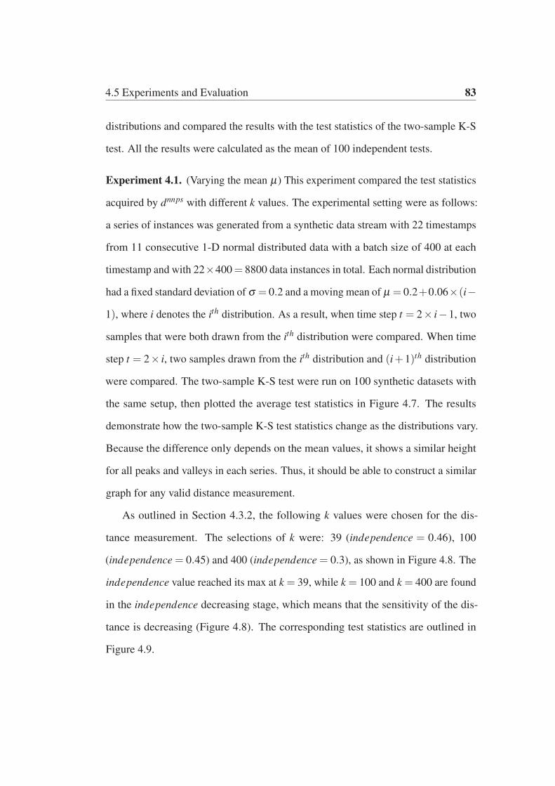
4.5 Experiments and Evaluation 83
distributions and compared the results with the test statistics of the two-sample K-S
test. All the results were calculated as the mean of 100 independent tests.
Experiment 4.1. (Varying the mean μ) This experiment compared the test statistics
acquired by dnnps with different k values. The experimental setting were as follows:
a series of instances was generated from a synthetic data stream with 22 timestamps
from 11 consecutive 1-D normal distributed data with a batch size of 400 at each
timestamp and with 22×400= 8800 data instances in total. Each normal distributionhad a fixed standard deviation of σ = 0.2 and a moving mean of μ = 0.2+0.06×(i−1), where i denotes the ith distribution. As a result, when time step t = 2× i−1, twosamples that were both drawn from the ith distribution were compared. When time
step t = 2× i, two samples drawn from the ith distribution and (i+1)th distribution
were compared. The two-sample K-S test were run on 100 synthetic datasets with
the same setup, then plotted the average test statistics in Figure 4.7. The results
demonstrate how the two-sample K-S test statistics change as the distributions vary.
Because the difference only depends on the mean values, it shows a similar height
for all peaks and valleys in each series. Thus, it should be able to construct a similar
graph for any valid distance measurement.
As outlined in Section 4.3.2, the following k values were chosen for the dis-
tance measurement. The selections of k were: 39 (independence = 0.46), 100
(independence = 0.45) and 400 (independence = 0.3), as shown in Figure 4.8. The
independence value reached its max at k = 39, while k = 100 and k = 400 are found
in the independence decreasing stage, which means that the sensitivity of the dis-
tance is decreasing (Figure 4.8). The corresponding test statistics are outlined in
Figure 4.9.

84 Concept Drift Detection via Accumulating Regional Density Discrepancies
1 2 3 4 5 6 7 8 9 10 11 12 13 14 15 16 17 18 19 20 21timestep
0
0.05
0.1
0.15
0.2
test
sta
tistic
Two Sample K-S Test
Figure 4.7 The test statistics of two-sample K-S test between normal distributed data withvarying μ . We compared two i.i.d. sample sets for each odd time step, and two sample setswith a drifted mean (μ +0.06) for each even time step. All the test statistics were computedbased on the average of 100 runs.
0 100 200 300 400 500 600 700 800Selection of k
0
0.2
0.4
0.6
0.8
1
inde
pend
ence
k=39 k=100
k=400
Figure 4.8 The relationship between independence and the selection of k

4.5 Experiments and Evaluation 85
1 2 3 4 5 6 7 8 9 10 11 12 13 14 15 16 17 18 19 20 21timestep
0
0.05
0.1
0.15
0.2
0.25te
st s
tatis
tic
Two Sample K-S Test dnnps k=39 dnnps k=100 dnnps k=400
Figure 4.9 The dnnps between normal distributed data (400 instances each time step) with
varying μ . We compared two i.i.d. sample sets for each odd timestep and two sample setswith a drifted mean (μ + 0.06) for each even timestep. All the statistics were computedbased on the average of 100 runs.
1 2 3 4 5 6 7 8 9 10 11 12 13 14 15 16 17 18 19 20 21timestep
0.1
0.15
0.2
0.25
test
sta
tistic
Two Sample K-S Test dnnps k=17
Figure 4.10 The dnnps between normal distributed data (50 instances each time step) with
varying μ .
The dnnps has the same pattern as the two-sample K-S test. The test statistic
values are smaller for larger k values (shown in blue). This is because larger k
values have a larger number of instance particles. Therefore, the ratio between the
intersection set and union set will decrease. Even though the test statistic means are
different, this will not affect the discrepancy measurement as long as the peak-valley
difference between the data structures is correctly reflected.
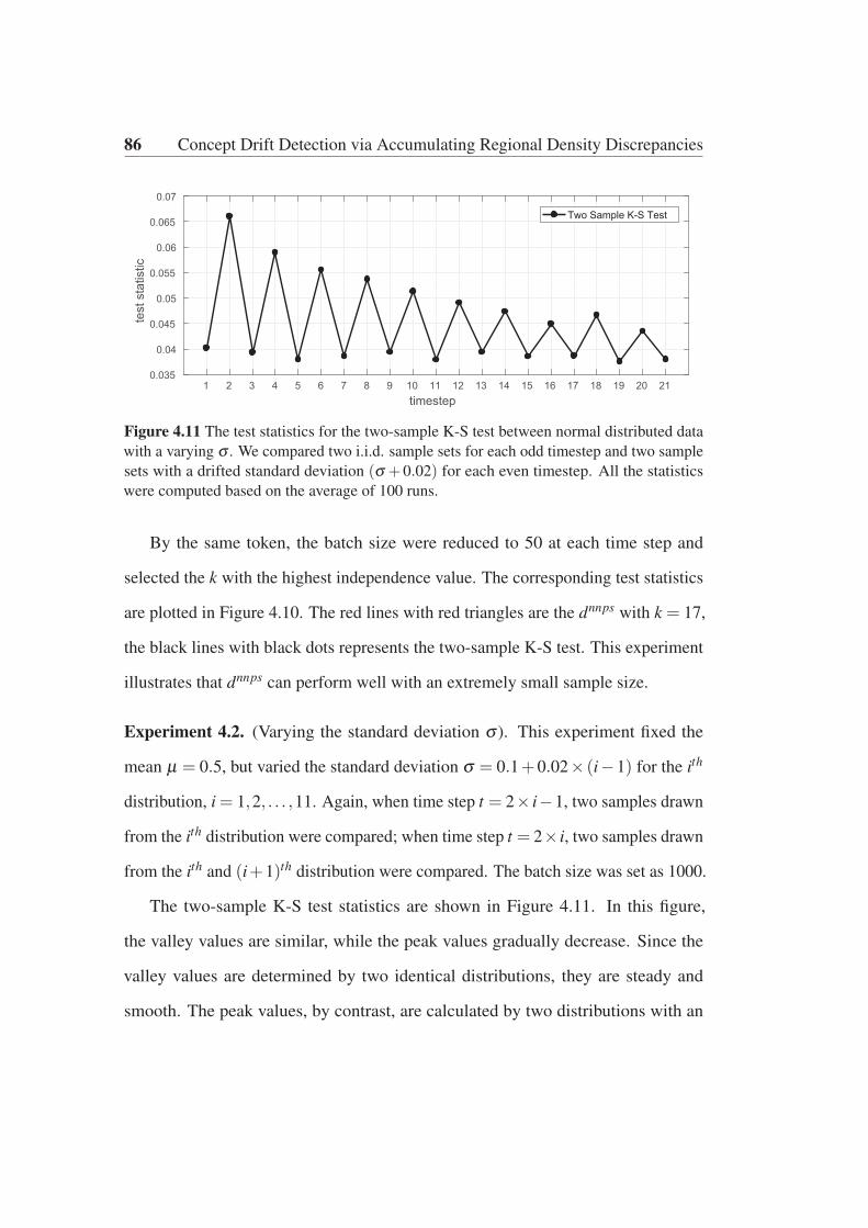
86 Concept Drift Detection via Accumulating Regional Density Discrepancies
1 2 3 4 5 6 7 8 9 10 11 12 13 14 15 16 17 18 19 20 21timestep
0.035
0.04
0.045
0.05
0.055
0.06
0.065
0.07
test
sta
tistic
Two Sample K-S Test
Figure 4.11 The test statistics for the two-sample K-S test between normal distributed datawith a varying σ . We compared two i.i.d. sample sets for each odd timestep and two samplesets with a drifted standard deviation (σ +0.02) for each even timestep. All the statisticswere computed based on the average of 100 runs.
By the same token, the batch size were reduced to 50 at each time step and
selected the k with the highest independence value. The corresponding test statistics
are plotted in Figure 4.10. The red lines with red triangles are the dnnps with k = 17,
the black lines with black dots represents the two-sample K-S test. This experiment
illustrates that dnnps can perform well with an extremely small sample size.
Experiment 4.2. (Varying the standard deviation σ ). This experiment fixed the
mean μ = 0.5, but varied the standard deviation σ = 0.1+0.02× (i−1) for the ith
distribution, i = 1,2, . . . ,11. Again, when time step t = 2× i−1, two samples drawnfrom the ith distribution were compared; when time step t = 2× i, two samples drawn
from the ith and (i+1)th distribution were compared. The batch size was set as 1000.
The two-sample K-S test statistics are shown in Figure 4.11. In this figure,
the valley values are similar, while the peak values gradually decrease. Since the
valley values are determined by two identical distributions, they are steady and
smooth. The peak values, by contrast, are calculated by two distributions with an

4.5 Experiments and Evaluation 87
1 2 3 4 5 6 7 8 9 10 11 12 13 14 15 16 17 18 19 20 21timestep
0
0.05
0.1
0.15
0.2
0.25
0.3
0.35te
st s
tatis
tic
Two Sample K-S Test dnnps k=50 dnnps k=100 dnnps k=400
Figure 4.12 The dnnps between normally distributed data that varies σ .
increasing σ . As a result, the difference between these distributions will shrink as σ
increases. Intuitively, this is because the distribution becomes less concentrated, thus
the relative test statistic is smaller. The test statistics for dnnps are shown in Figure
4.12, where it can be seen that dnnps has the same pattern as the two-sample K-S test,
indicating that dnnps is capable of precisely representing differences in distribution.
Experiment 4.3. (Varying the regional mean μ j). This experiment compared the
distances between two data samples that comprise 30 independent 1-D normal
distributed data groups. In the first data group, the normal distribution was set as
μ = 0.2, σ = 0.2. The normal distribution was set as μ = 0.2+ j×(20×σ), σ = 0.2
for j = 2,3, . . . ,30 for the remaining 29 data groups. A (20×σ) gap between each
group was intentionally kept to ensure that a change occurring in one group would
not affect the others. Each group contained 100 data instances, equating to 3000
instances for each time step. In the first time step, two data sample sets without any
drift were compared . Later, the mean of each data group was manually changed by
μ j +0.06 successively for each time step to create 30 minor regional drifts.

88 Concept Drift Detection via Accumulating Regional Density Discrepancies
0 1 2 3 4 5 6 7 8 9 10 11 12 13 14 15 16 17 18 19 20 21 22 23 24 25 26 27 28 29 30 31timestep
0
0.05
0.1
0.15
0.2
0.25
0.3
0.35
test
sta
tistic
Two Sample K-S Test dnnps k=35
pValue = 0.9999
pValue = 0.024pValue = 0.232
Figure 4.13 1-D normal distribution with regional drift detection. At each timestep, themean (μ +0.06) of a group of data instances was changed, and the dnnps between the current
timestep and last timestep was plotted. The proposed dnnps reported a significant difference
at after 19 groups drifted, whereas the K-S test cannot detect such a difference.
Figure 4.13 shows the test statistics for the two-sample K-S test and the dnnps
at different time steps. At t = 1, 30 data groups with another 30 groups that were
generated by the same distribution were compared . At t = 2, the algorithm compared
30 data groups with another 29+ 1 groups where the mean μ1 of group 1 was
changed to μ1+ 0.06, and so on until t = 31. It can clearly be seen that dnnps
increased after each local drift occurred. In fact, the K-S test statistics also slightly
increased. However, the trend cannot be observed in this figure as the value of the
test statistic is too small. In addition, the algorithm also applied the corresponding
significance test to compare the test statistics and examine whether the drifts were
statistically significant. The p-value of the two-sample K-S test was above 95% the
entire time, while the p-value of dnnps dropped below 5% after time step 19, which
means that dnnps can detect simulated drifts after 19/30 local drifts. This experiment
demonstrates that the proposed dnnps is sensitive to regional drifts.

4.5 Experiments and Evaluation 89
4.5.2 Evaluating the NN-DVI drift detection accuracy
In the above experiment, it has shown how dnnps varies as the underlying distribution
changes. To determine whether a given measurement is a statistically significant drift,
the ASL as described in Section 4.4.2 was computed. Given a desired significance
level α , the system would say there is a concept drift when the ASL< α . In the
following experiments, NN-DVI was compared with Dasu et al. (2006) and Lu et al.
(2014) in terms of drift detection accuracy on ten synthetic data streams. The reason
these two algorithms were chosen for comparison is that all three methods, including
NN-DVI, detect concept drift based on the estimated data distribution without holding
any assumptions about those distributions. Additionally, one of the most popular
two-sample tests for multivariate data as a baseline – Maximum Mean Discrepancy
(MMD) Gretton et al. (2012) was also compared. NN-DVI(permutation) denotes
the use of a permutation test to estimate the ASL of NN-DVI, and NN-DVI(normal)
denotes the use of the tailored significance test that has been proven following normal
distribution to calculate the ASL of NN-DVI.
For fair comparison, the same experimental configurations and evaluation criteria
were used as introduced in Dasu et al. (2006) and Lu et al. (2014). The evaluation
criteria are: detected, late, f alse, and missed. A concept exists for a period of time
[t +1, t + z], where z is the length of the concept. In this experiment, the distribution
parameters were updated at t + 1 and t + z+ 1, that is, a new concept starts from
t + 1 and ends at t + z. Each time step involves three processes: three processes:
updating distribution parameters if new concept starts, generating data, and detecting
drift. Detected indicates the number of times the drift detection algorithm reports a
drift at t +1. Late indicates the number of times a drift is reported at t +2 or t +3.

90 Concept Drift Detection via Accumulating Regional Density Discrepancies
False accumulates the number of false alarms that multiple drifts are reported in
[t +1, t + z]. A missed detection is counted if no drift is reported within [t +1, t +3].
A detected drift within [t + 4, t + z] is marked as missed because such a detection
is considered to be too late to be useful Lu et al. (2014). Dasu et al.’s algorithm is
denoted as KL (Kullback-Leibler distance) and Lu et al.’s work is denoted as CM
(competence model). With regard to the data source, the same synthetic datasets
introduced by Dasu et al. (2006) and adopted by Lu et al. (2014) were implemented.
5 million data instances for each data stream were generated, and for every 50,000
instances, the parameters of the corresponding distribution were varied randomly
within a certain interval. These variations produced 99 controllable drifts for each
data stream. For ease of comparison, all the parameters were kept the same for both
the bootstrapping test and the permutation test, including the desired significance
level of α = 1%, and the size of bootstrapping and permutation N = 500. KL and
CM’s parameters were set as per their papers. Euclidean distance is used as the
distance function in this section as this is the distance measure used in Dasu et al.
(2006); Lu et al. (2014). Because the permutation test does not hold any assumptions
and can be applied to KL without modification, KL with a permutation test was
also included for comparison. To avoid any bias in NN-DVI caused by parameter
selection, we first conducted an experiment with a k-value that was chosen based
on the average number of instances within the same partitioning size as KL and
CM. Then, we ran our algorithm with a dynamic k-value that was selected based
on maxk
{independence} and applied the normal distribution estimation described inSection 4.4.2.2 as the significance test.
4.5 Experiments and Evaluation 91
Experiment 4.4. (Normal distributions). In this experiment, KL, CM, and NN-DVI
were compared using five bivariate normal distributed data streams, denoted as
M(�) and C(�) streams. Drift severity was controlled by a predefined drift margin
�. In the M(�) streams, the features x1 and x2 followed an independent normal
distribution, with the means μ1 and μ2 moving within [0.2,0.8]. For every 50,000
instances, μ1 and μ2 were randomly updated with a step size [−�,−�/2∪ [�/2,�].
In theC(�) streams, the two features have a moving correlation ρ , which started at
0 and was then randomly walked within [−1,1], with a step size chosen randomlyfrom [−�,−�/2]∪ [�/2,�]. To investigate the impact of the window size on drift
detection accuracy, the experiment was conducted on theC(0.15) stream with two
different window sizes. All the results are summarized in Tables 4.1 and 4.2.
The results demonstrate that our method outperformed the others in most cases.
In terms of the false and missed rates, only bootstrapped KL on theC(0.2) stream
was slightly better than ours. With regard to the other streams, our results were
much better. When considering drift detection based on permutation tests, no other
tested methods can surpass ours. The results show that the excellent performance
of KL with bootstrap is most likely attributed to the bootstrap test rather than to
their drift detection model. Nevertheless, Dasu et al. Dasu et al. (2006) did not
give any explanation for their selection of the significance test, rather they only
suggest researchers investigate the pros and cons in other publications. It is also
noteworthy that all the detection algorithms achieved high detection rates onM(0.05)
and C(0.2). According to the data generation settings, M(0.05) and C(0.2) have
relatively large drift margins. This would make the drifts easier to detect, and the
drift detection results may be very similar as long as the drift margins exceed the
sensitivity thresholds of the tested algorithms. For example, in this experiment,

92ConceptDriftDetectionviaAccumulatingRegionalDensityDiscrepancies
Table 4.1 NN-DVI drift detection results on M(�) stream
Data Stream Drift Detection Method Parameters Window Size Detected Late False Missed
M(0.02) KL (bootstrap) δ : 2−10,τ : 100,γ : 5% 10000 76 13 2 10
KL (permutation) δ : 2−10,τ : 100,γ : 5% 10000 68 14 3 17
CM (permutation) dε : 0.05 10000 87 5 12 7
NN-DVI (permutation) k : 185 10000 90 8 9 1
NN-DVI normal) k : max{independence} 10000 91 6 6 2
MMD RBF kernel, σ = 0.23 10000 99 0 3 0
M(0.05) KL (bootstrap) δ : 2−10,τ : 100,γ : 5% 10000 99 0 9 0
KL (permutation) δ : 2−10,τ : 100,γ : 5% 10000 99 0 3 0
CM (permutation) dε : 0.05 10000 99 0 2 0
NN-DVI (permutation) k : 185 10000 99 0 5 0
NN-DVI (normal) k : max{independence} 10000 99 0 5 0
MMD RBF kernel, σ = 0.23 10000 99 0 3 0
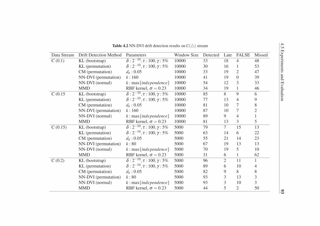
4.5Experim
entsandEvaluatio
n93
Table 4.2 NN-DVI drift detection results onC(�) stream
Data Stream Drift Detection Method Parameters Window Size Detected Late FALSE Missed
C (0.1) KL (bootstrap) δ : 2−10,τ : 100,γ : 5% 10000 33 18 4 48
KL (permutation) δ : 2−10,τ : 100,γ : 5% 10000 30 16 1 53
CM (permutation) dε : 0.05 10000 33 19 2 47
NN-DVI (permutation) k : 160 10000 41 19 0 39
NN-DVI (normal) k : max{independence} 10000 54 12 3 33
MMD RBF kernel, σ = 0.23 10000 34 19 1 46
C (0.15 KL (bootstrap) δ : 2−10,τ : 100,γ : 5% 10000 85 8 9 6
KL (permutation) δ : 2−10,τ : 100,γ : 5% 10000 77 13 4 9
CM (permutation) dε : 0.05 10000 81 10 7 8
NN-DVI (permutation) k : 160 10000 87 10 7 2
NN-DVI (normal) k : max{independence} 10000 89 9 4 1
MMD RBF kernel, σ = 0.23 10000 81 13 3 5
C (0.15) KL (bootstrap) δ : 2−10,τ : 100,γ : 5% 5000 79 7 15 13
KL (permutation) δ : 2−10,τ : 100,γ : 5% 5000 63 14 6 22
CM (permutation) dε : 0.05 5000 55 21 14 23
NN-DVI (permutation) k : 80 5000 67 19 13 13
NN-DVI (normal) k : max{independence} 5000 70 19 5 10
MMD RBF kernel, σ = 0.23 5000 31 6 1 62
C (0.2) KL (bootstrap) δ : 2−10,τ : 100,γ : 5% 5000 96 2 11 1
KL (permutation) δ : 2−10,τ : 100,γ : 5% 5000 89 6 10 4
CM (permutation) dε : 0.05 5000 82 9 8 8
NN-DVI (permutation) k : 80 5000 93 3 13 3
NN-DVI (normal) k : max{independence} 5000 93 3 10 3
MMD RBF kernel, σ = 0.23 5000 44 5 2 50

94 Concept Drift Detection via Accumulating Regional Density Discrepancies
the drift margins for M(0.05) exceeded the sensitivity threshold of all the tested
algorithms. Therefore, all the results were very close (the missed rates were all zero,
and the f alse rates were all low). We infer that the C(0.2) reached a sensitivity
threshold of both KL with bootstrap and NN-DVI. Unlike the M(0.05) andC(0.2)
streams, the rest of the streams had smaller drift margins. The high detection rates
on those streams prove that NN-DVI is more sensitive to small concept drifts.
Experiment 4.5. (Poisson distributions). In P(�) streams, the two features follow
a Poisson distribution Poisson(500(1−ρ),500(1−ρ),500ρ), where ρ starts at 0.5
and then performs a random walk between 0 and 1 with step size�= 0.2,0.1. The
evaluation results are shown in Table 4.3.
Table 4.3 shows that KL using a bootstrap test suffers a manifest failure on
Poisson distributions. On the one hand, KL using a permutation test detected most
drifts correctly on P(0.2). It is evident that the P(0.2) drift margin was larger than
the KL sensitivity threshold. On the other hand, KL suffered high f alse rate on
P(0.2) when combined with the bootstrap test. This paradox indicates how a null
hypothesis test could affect the sensitivity of a drift detection algorithm, and the
bootstrap test may not be suitable for the KL algorithm in all circumstances. In
general, according to the results in Table 4.3, NN-DVI clearly outperformed the
others.
Experiment 4.6. (Higher dimensional distributions). To test the scalability and
performance of NN-DVI in high-dimension space, the C(0.2) stream is extended to
d-4, d-6 and d-10 multivariate normal distributed streams as per Dasu et al. (2006);
Lu et al. (2014). Only the first two dimensions had a correlation value equal to ρ ; the
remaining (d-2) dimensions were configured with correlation values equal to zero.

4.5Experim
entsandEvaluatio
n95
Table 4.3 NN-DVI drift detection results on P(�) stream
Data Stream Drift Detection Method Parameters Window Size Detected Late False Missed
P(0.1) KL (bootstrap) δ : 2−10,τ : 100,γ : 5% 10000 64 7 1 28
KL (permutation) δ : 2−10,τ : 100,γ : 5% 10000 66 8 4 25
CM (permutation) dε : 10 10000 63 8 1 28
NN-DVI (permutation) k : 545 10000 81 7 7 11
NN-DVI (normal) k : max{independence} 10000 81 9 5 9
MMD RBF kernel, σ = 0.23 10000 61 8 2 30
P(0.2) KL (bootstrap) δ : 2−10,τ : 100,γ : 5% 10000 95 1 11 3
KL (permutation) δ : 2−10,τ : 100,γ : 5% 10000 98 0 1 1
CM (permutation) dε : 10 10000 99 0 5 0
NN-DVI (permutation) k : 545 10000 99 0 6 0
NN-DVI (normal) k : max{independence} 10000 99 0 6 0
MMD RBF kernel, σ = 0.23 10000 98 1 10 0

96 Concept Drift Detection via Accumulating Regional Density Discrepancies
Additionally, the standard deviation of all the added dimensions was configured to
be the same as theC(�) streams. These settings were managed to retain the same
marginal distribution of all dimensions, so that the overall distance between the
instances contributed by each dimension was equally important Dasu et al. (2006);
Lu et al. (2014). Thus, it was easier to calculate the distance between instances, and
the drift detection results were not affected by the selection of the distance functions
used to compare the data instances.
The experimental results for different dimensions are listed in Table 4.4. As
expected, as more stationary dimensions were added, the missed rates of all detection
algorithms increased, implying that such a change makes drift detection more difficult.
However, NN-DVI preserves much of its power as the number of dimension increases.
It is very likely that this can be attributed to the k-nearest neighbor-based model
defined in Section 4.3.2.
To summarize, we calculated the average detected, late, f alse and missed rates
of all synthetic streams, as shown in Table 4.5. The results show that the proposed
NN-DVI makes a notable improvement to drift detection in various situations. Al-
though the f alse rate of NN-DVI was slightly higher than the existing methods
with the permutation test, the missed rate was almost halved. The performance of
NN-DVI with a normal distribution as the significance test is even better. It shows a
higher detected rate with a lower f alse rate, which indicates the tailored significance
test introduced in Section 4.4.2.2 is more reliable. In addition, the complexity of
the model construction can be reduced to O(knlog(n)) with a kd-Tree data structure,
while CM is O(n2log(n)) Lu et al. (2014), KL is O(dnlog(1/δ )) where the d is the

4.5Experim
entsandEvaluatio
n97
Table 4.4 NN-DVI drift detection results on HDC(�) streams
Data Stream Drift Detection Method Parameters Window Size Detected Late False Missed
4D C(0.2) KL (bootstrap) δ : 2−10,τ : 100,γ : 5% 10000 91 5 5 3
KL (permutation) δ : 2−10,τ : 100,γ : 5% 10000 87 8 5 4
CM (permutation) dε : 0.15 10000 89 3 8 7
NN-DVI (permutation) k : 95 10000 94 5 5 0
NN-DVI (normal) k : max{independence} 10000 95 4 6 0
MMD RBF kernel, σ = 0.23 10000 83 10 2 6
6D C(0.2) KL (bootstrap) δ : 2−10,τ : 100,γ : 5% 10000 84 5 6 10
KL (permutation) δ : 2−10,τ : 100,γ : 5% 10000 65 11 3 23
CM (permutation) dε : 0.3 10000 91 4 7 4
NN-DVI (permutation) k : 200 10000 97 2 6 0
NN-DVI (normal) k : max{independence} 10000 95 4 6 0
MMD RBF kernel, σ = 0.23 10000 69 12 7 18
10D C(0.2) KL (bootstrap) δ : 2−10,τ : 100,γ : 5% 10000 81 7 4 11
KL (permutation) δ : 2−10,τ : 100,γ : 5% 10000 68 13 5 18
CM (permutation) dε : 0.5 10000 78 10 4 11
NN-DVI (permutation) k : 220 10000 89 5 3 5
NN-DVI (normal) k : max{independence} 10000 88 6 5 5
MMD RBF kernel, σ = 0.23 10000 26 18 0 55

98 Concept Drift Detection via Accumulating Regional Density Discrepancies
Table 4.5 NN-DVI average drift detection results
Drift Detection Method Detected Late FALSE Missed
KL (bootstrap) 80.27 6.64 7 12.09
KL (permutation) 73.64 9.36 4.09 16
CM (permutation) 77.91 8.09 6.36 13
NN-DVI (permutation) 85.18 7.09 6.73 6.73
NN-DVI (normal) 86.73 6.55 5.82 5.73MMD 65.91 8.36 3.09 24.73
number of data dimensions and δ is the given parameter of KL Dasu et al. (2006),
and MMD is O(n2) Gretton et al. (2012).
4.5.3 Evaluating the NN-DVI on real-world datasets
To demonstrate how our drift detection algorithm improves the performance of
learning models in real-world scenarios, we again compared our detection method
with KL Dasu et al. (2006) and CM Lu et al. (2014)), this time, on five benchmark
real-world concept drift datasets. These datasets are the top referenced benchmark
datasets and include both low- and high-dimensionality data. Additionally, we also
compared NN-DVI with four state-of-the-art drift adaptation algorithms that address
concept drift using different strategies. These algorithms are: SAMkNN Losing
et al. (2016), which keeps past concepts in memory and considers all buffered con-
cepts to make a final prediction; AUE2 Brzezinski and Stefanowski (2014), which
uses ensemble methods to handle concept drift; HDDM family tests (HDDM-A,
HDDM-W) Frias-Blanco et al. (2015), which detects drift by monitoring learner
outputs; and ADWIN-Volatility (ADW-Vol) Huang et al. (2015) which first intro-
duced volatility shift into concept drift detection. Lastly, we selected HAT Bifet and
Gavaldà (2009) and ADWIN Bifet and Gavaldà (2007) as baselines. The algorithms

4.5 Experiments and Evaluation 99
were implemented using the authors’ recommended settings. The selection of the
base learners for the HDDM family tests, KL, CM, and NN-DVI is independent
of the drift detection algorithm. Therefore, we implemented these algorithms with
Naïve Bayes, Hoeffding Tree, and IBk classifiers. Because the SAMkNN is only
compatible with IBk, and AUE2 is only compatible with Hoeffding Tree, these two
algorithms were only compared with their own base learners. All algorithms were
implemented based on the MOA platform Bifet et al. (2010a), which is written in
Java. The parameters for IBk were set as k = 5, and instances weighting method was
uni f ormly weighted. All the distance functions used in this section are Euclidean.
The Heoffding Tree parameters were set as recommended by AUE2. Table 4.6
summarizes the classification accuracy and gives the overall rank of the different
algorithms. The average processing time in seconds and the average memory usage
(RAM-Hour in Gigabyte) are also listed since computational resources management
is an important issue in data stream learning Bifet et al. (2010c).
Experiment 4.7. (Electricity Price Prediction) The electricity dataset contains
45,312 instances, collected every 30 minutes from the Australian New South Wales
Electricity Market between 7 May 1996 and 5 Dec 1998. In this market, prices are
not fixed but are affected by supply and demand. This dataset contains eight features
and two classes (up, down) and has been widely used for concept drift adaptation
evaluation Frias-Blanco et al. (2015); Losing et al. (2016). The dataset is available
from MOA’s website Bifet et al. (2010a)
Experiment 4.8. (Spam Filtering)This dataset is a collection of 9324 email mes-
sages derived from the Spam Assassin collection, available online1. The original
1http://spamassassin.apache.org/

100 Concept Drift Detection via Accumulating Regional Density Discrepancies
dataset contains 39,916 features and 9324 emails (around 20% spam emails and 80%
legitimate emails). It is commonly considered to be a typical gradual drift dataset
Katakis et al. (2009). Katakis Katakis et al. (2009) retrieved 500 attributes, using the
Chi-square feature selection approach.
Experiment 4.9. (Weather Prediction) The Nebraska weather prediction dataset was
compiled by the US National Oceanic and Atmospheric Administration. It contains
8 features and 18,159 instances with 31% positive (rain) classes, and 69% negative
(no-rain) classes. This dataset is summarized in Elwell and Polikar (2011) and is
available online2
Experiment 4.10. (Usenet1 and Usenet2) The Usenet datasets were first introduced
by Katakis et al. (2008) and were used to evaluate HDDM family algorithms Frias-
Blanco et al. (2015). They are two subsets of the Twenty Newsgroups collection,
which is owned by the UCI Machine Learning Repository. Each dataset consists
of 1500 instances and 99 features. In these datasets, each instance is a message
from different newsgroups that are sequentially presented to a user, who then labels
the messages as interesting or not interesting. These messages involve three topics:
medicine, space, and baseball. The user was simulated with a drifted interest every
300 messages. A more detailed explanation of these datasets can be found in Katakis
et al. (2008).
To better demonstrate the improvements NN-DVI can make in tackling real-
world problems, we used a ranking method to summarize its overall performance,
similar to Losing et al. (2016). The average rank shows that NN-DVI achieved the
2http://users.rowan.edu/ polikar/research/NSE
4.5 Experiments and Evaluation 101
best performance with the IBk classifier and had the best final score as an average of
all the base classifier ranks.
The analysis results of Table 4.6 can be summarized as follows:
• The performance of the base learners varied on different datasets. For ex-
ample, under the same drift adaptation algorithm, the IBk classifier always
outperformed the other classifiers on the Weather dataset, and it performed the
worst on the Usenet1 and Usenet2 datasets. In some situations, the selection
of base learners may be more important than the selection of drift detection
methods. This outcome inspired us to reconsider the learning strategy of
using the same base classifier settings after a drift. Instead, changing a base
learner or updating the base learner’s parameters may further improve overall
prediction accuracy.
• The proposed NN-DVI method with IBk, NB, and HTree had the best per-
formance in terms of accuracy. Considering the overall performance, it is
evident that the highlighted results of NN-DVI do not depend on the base
classifiers and that NN-DVI contributes to the learning process in a dynamic
environment.
• Regarding computational complexity, it can be seen that the distribution-
based drift detection algorithms (NN-DVI, CM, and KL) have very similar
computational costs, namely the Time and RAM-Hour, for all the tested
three-base learners. The reason is that these algorithms have to keep the
representative data instances in memory to detect the distribution changes.
This appears to be a common issue for distribution-based drift detection
methods. Nevertheless, they have shown no manifest disadvantages over other

102
ConceptDriftDetectionviaAccumulatingRegionalDensityDiscrepancies
Table 4.6 NN-DVI Classification accuracy of real-world datasets. The rank of each algorithm is shown in brackets. The final score is theaverage rank of that algorithm combined with different base learners. The time(s) and RAM-Hour (GB) are calculated based on the
average of the five datasets.
Algorithms Learner Elec Spam Weather Usenet1 Usenet2 AVG. Rank Score Time RAM-Hour
NB 84.10 (6) 92.03 (9) 72.50 (12) 68.93 (12) 77.13 (2) 8.2 (2) 190.6 2.85E-05
NN-DVI IBk 87.39 (2) 93.47 (2) 74.63 (7) 66.80 (17) 72.47 (7) 7.0 (1) 2.0 (1) 208.5 2.85E-05
HTree 82.85 (10) 92.06 (8) 71.68 (17) 70.27 (9) 76.73 (4) 9.6 (3) 195.2 2.85E-05
SAMkNN IBk 82.54 (14) 95.67 (1) 78.26 (1) 66.13 (19) 70.33 (17) 10.4 (5) 5.0 (2) 266.5 3.75E-02
NB 84.09 (7) 91.65 (14.5) 72.82 (11) 75.07 (2) 70.93 (16) 10.1 (4) 1.4 4.91E-08
HDDM-W IBk 82.47 (15) 92.93 (3) 75.04 (6) 69.67 (10) 67.93 (22) 11.2 (10) 6.7 (3) 249.9 2.07E-03
HTree 85.06 (4) 91.65 (14.5) 72.41 (13) 74.73 (3) 70.00 (18) 10.5 (6) 1.4 7.52E-08
NB 84.92 (5) 90.79 (20) 72.38 (14) 75.20 (1) 71.00 (14.5) 10.9 (8) 1.4 4.97E-08
HDDM-A IBk 82.10 (16) 92.00 (10) 76.13 (4) 69.33 (11) 68.00 (21) 12.4 (11.5) 9.5 (4) 132.2 1.05E-04
HTree 85.71 (3) 91.78 (13) 71.71 (16) 74.60 (4) 68.87 (19.5) 11.1 (9) 1.6 7.55E-08
NB 82.66 (12) 91.10 (19) 71.89 (15) 71.07 (7) 77.20 (1) 10.8 (7) 137.2 4.54E-04
CM IBk 78.98 (23) 89.34 (23) 73.71 (8) 67.47 (14) 71.33 (13) 16.2 (23) 14.7 (5) 133.3 4.54E-04
HTree 81.33 (20) 91.11 (18) 71.23 (20) 71.73 (5) 76.27 (5) 13.6 (14) 144.8 4.54E-04
NB 82.62 (13) 91.19 (16) 71.00 (22) 70.73 (8) 77.06 (3) 12.4 (11.5) 191.7 7.90E-05
KL IBk 78.95 (24) 89.37 (22) 73.68 (9) 67.27 (15) 71.00 (14.5) 16.9 (24) 16.8 (6) 186.7 7.91E-05
HTree 81.34 (19) 91.16 (17) 71.18 (21) 71.33 (6) 76.20 (6) 13.8 (15) 171.7 7.94E-05
NB 80.64 (22) 91.83 (12) 71.40 (18) 68.13 (13) 72.27 (8.5) 14.7 (21) 1.3 5.73E-08
ADW-Vol IBk 81.72 (18) 92.81 (4) 76.20 (2.5) 59.73 (23.5) 67.27 (23.5) 14.3 (17.5) 17.2 (7) 201.5 5.93E-05
HTree 82.84 (11) 92.59 (5) 71.28 (19) 66.67 (18) 72.00 (10.5) 12.7 (13) 1.5 9.28E-08
AUE2 HTree 87.74 (1) 84.29 (24) 75.24 (5) 63.47 (22) 68.87 (19.5) 14.3 (17.5) 17.5 (8) 4.4 5.37E-06
HAT HTree 83.39 (8) 90.69 (21) 73.51 (10) 63.93 (21) 71.87 (12) 14.4 (19) 19.0 (9) 2.0 7.92E-08
NB 81.03 (21) 91.90 (11) 70.31 (24) 67.00 (16) 72.27 (8.5) 16.1 (22) 1.4 5.04E-08
ADWIN IBk 81.76 (17) 92.46 (6) 76.20 (2.5) 59.73 (23.5) 67.27 (23.5) 14.5 (20) 19.3 (10) 200.7 5.63E-05
HTree 83.23 (9) 92.29 (7) 70.88 (23) 64.47 (20) 72.00 (10.5) 13.9 (16) 1.4 7.90E-08

4.5 Experiments and Evaluation 103
drift detection methods using IBk learner. Although error rate-based and
ensemble-based drift adaptation methods can handle concept drift in an online
manner, using IBk as the base learner may slow down their learning speeds.
4.5.4 Evaluating the stream learning with NN-DVI with differ-
ent parameters
Generally, the algorithm for stream learning with NN-DVI has six input parameters:
1) the minimum drift detection window size; 2) the base learner; 3) the distance
function for constructing NNPS; 4) the number of nearest neighbors for NNPS;
5) the sampling time to estimate the σ of dnnps; and 6) the drift significance level.
Parameter 2 is evaluated in Section 4.5.3; parameter 4 is discussed in Section 4.3.2;
parameter 5 is related to the Monte Carlo Error, which has been detailed in Section
5.2 of Lu et al. (2014); and parameter 6 is a drift sensitivity setting chosen by the
user and is highly dependent on system requirements. Therefore, in this section, we
focus on evaluating the impact of parameter 1, the minimum drift detection window
size, and parameter 3, the distance function for constructing NNPS. The rest of the
parameters are fixed at the default values.
Experiment 4.11. (Varying window size) As a critical parameter of time window-
based drift detection algorithms, the window size, or chuck size Shao et al. (2014)
controls the length of the most recent concept, namely the winslide in our algorithm.
If the window size is too small, the most recent concept may be incomplete and a
false alarm will be raised. If the window size is too large, multiple concepts may be
included in one window, which would lead to bad performance. To evaluate how

104
ConceptDriftDetectionviaAccumulatingRegionalDensityDiscrepancies
50 100 150 200 250window size
65
70
75
80
85
90
accu
racy
(%)
(a) Elec dataset
Euc Man Che Jac RBF
50 100 150 200 250window size
75
80
85
90
95
accu
racy
(%)
(b) Spam dataset
Euc Man Che Jac RBF
50 100 150 200 250window size
66
68
70
72
74
76
78
accu
racy
(%)
(c) Weather dataset
Euc Man Che Jac RBF
50 100 150 200 250window size
50
55
60
65
70
accu
racy
(%)
(d) Usenet1 dataset
Euc Man Che Jac RBF
50 100 150 200 250window size
66
67
68
69
70
71
72
73
accu
racy
(%)
(e) Usenet2 dataset
Euc Man Che Jac RBF
0 50 75 100 150 250window size
65
70
75
80
85
accu
racy
(%)
(f) Average Accuracy of Five DatasetsEuc Man Che Jac RBF
Figure 4.14 Classification accuracy of real-world datasets with different window size and different distance functions. Each linerepresents a distance function. A marker on a line represents the classification accuracy of NN-DVI with a given distance function and
on the window size. (f) shows the average accuracy of the tested five datasets for each distance function with different window size.

4.6 Summary 105
window size affects NN-DVI, we set winmin =50, 75, 100, 150, 200, and plotted the
classification accuracy of the five real-world datasets, as shown in Figure 4.14.
Experiment 4.12. (Changing distance functions) To evaluate how different distance
functions for constructing NNPS affects NN-DVI on real-world datasets, we choose
another four most commonly used distance functions to replace Euclidean distance,
namely: Manhattan distance, Chebyshev distance, Jaccard distance, and Radial basis
function kernel distance. The overall classification accuracy of these distances with
different window size is plotted in Figure 4.14.
It can be seen in Figure 4.14 that an increase in window size correlates with a
decrease in average accuracy, especially for dataset Usenet1. This could be caused by
mixed concepts in time windows. The Spam and Weather dataset accuracies slightly
increased in line with window size, leading us to query if NN-DVI inappropriately
overly triggered false alarms because of the small window size of these datasets.
Increasing the window size should reduce the overall rate of false alarms and, hence,
increase the accuracy. The Euclidean and Manhattan distance functions performed
very similarly and were the top two functions for the evaluated datasets, while
Jaccard’s distance consistently performed the worst. Therefore, we recommend
Euclidean or Manhattan distances for most situations.
4.6 Summary
This chapter analyzed distribution-based drift detection algorithms and summarized
the fundamental components of this type of drift detection method. Under the
guidance of the summarized framework (Figure 4.1), this chapter proposed a novel

106 Concept Drift Detection via Accumulating Regional Density Discrepancies
space partitioning schema, called NNPS, to improve the sensitivity of regional
drift detection. Accordingly, a novel distance dnnps and a nearest neighbor-based
density variation identification (NN-DVI) algorithm were proposed. This research
also defined a k-nearest neighbor-based data discretization controlling method to
represent granular information in data samples. This chapter theoretically proved
the proposed distance measurement dnnps, fits a normal distribution. According to
this finding, an efficient and reliable critical interval identification method has been
integrated. The experimental results show that NN-DVI can detect concept drift
accurately in synthetic datasets and is beneficial for solving real-world concept drift
problems.
The innovation and contributions of this chapter lie in its aim to discover the re-
lationships between distribution drifts and the changes in neighboring data instances.
A regional density-oriented similarity measurement is given that can effectively
detect concept drift caused by either regional or global distribution changes.

Chapter 5
Concept Drift Adaptation via
Reginal Density Synchronization
5.1 Introduction
At present, most concept drift detection and handling methods are focusing on time-
related drift, namely when a concept drift occurs. They consider that a drift could
occur suddenly at a time point, incrementally, or gradually in a time period Harel
et al. (2014). As a result, their solutions are searching the best time to split the old
and new concepts. The data received before the drift time point is considered as old
concept, while the data received after is considered as new concept. Accordingly, the
old concept data is discarded, while new concept data is used for updating or training
new learners, which can be seen as a time-oriented “one-cut” process. However, in
real-world scenarios, this assumption is not always true. A concept drift could only
occur within some specific regions. Such a “one-cut” process does not consider the
non-drifted regions in the old concept. Although some algorithms have introduced a

108 Concept Drift Adaptation via Reginal Density Synchronization
buffer system to keep tracking drifting concepts and can find the best drift time point
to identify concepts, they are not able to retrieve the location information related to
the drifted regions Liu et al. (2017b).
For example, in real-world scenarios, one drift could be a mixture of all three
types of drifts Sarnelle et al. (2015). How to handle the intermediate concepts in
a drift is a challenging problem. So far, most the state-of-the-art drift detection
algorithms only detect when the intermediate concept drift. Very little research has
discussed the intermediate concepts from a spatial perspective, such as research on
where the drifted regions are. Considering both when and where a drift occurs is
beneficial to reduce the risk of overestimating the drift regions, as shown in Figure
5.1.
In one related publication Gama and Castillo (2006), the authors applied a deci-
sion tree model to detect changes in the online error-rate in each internal tree node,
thereby identifying drifted nodes and updating them, respectively. The experimental
results showed a good performance in detecting drift and in adapting the decision
model to the new concept. Similar algorithms are in Ikonomovska et al. (2011,
2015, 2009). However, these algorithms mainly focus on addressing concept drift
on regression problems and they all are based on decision tree models, which have
limited application areas.
To better address concept drift problems, we consider both time-related and
spatial-related drift information. In this paper, we propose a regional density inequal-
ity metric, called local drift degree (LDD), to measure the likelihood of regional
drift in every suspicious region. By analyzing the density increasing or decreasing
in a local region, learning systems are able to highlight dangerous regions and take
relevant actions.

5.1 Introduction 109
decision boundary (b)
decision boundary (c)
decision boundary (a)
decision boundary (a)
decision boundary (b)
decision boundary (c)
(a) decision boundary before concept drift (b) new decision boundary with regional drift detection
(c) new decision boundary after global drift detection
(d) overestimated drift regions
over estimated drift regionsactual drift region
decision boundary (a)
over estimated drift regionsactual drift region
decision boundary (a)
all historical data received before drift time step is discarded
data instances with different labels
data instances arrived at different time step
only drifted instances are discarded
Figure 5.1 For any notable concept drift, if the distribution difference is only in a smallregion, as shown in (b), discarding the entire historical data and retraining the learner
may result in a overestimation of the drift regions, such as the red shaded regions in (d),
and thereby impairing the overall performance. By contrast, regional drift detection and
adaptation only address targeted regions, and will not over estimate the drifts.

110 Concept Drift Adaptation via Reginal Density Synchronization
5.2 Local Drift Degree
In this section, we formally present the proposed test statistics, LDD. The purpose
of LDD is to quantify regional density discrepancies between two different sample
sets, thereby, identifying density increased, decreased and stable regions.
5.2.1 The definition of LDD
The intuitive idea underlying LDD is that, given two d-dimensions populations
Ad and Bd , if two sample sets, A from Ad and B from Ad , are independent and
identically distributed, their local density discrepancies follow a certain normal
distribution. Denote the feature space as V , for any subspaceW ⊆V , it has an it has
an equality that |AW |/nA �= |BW |/nB in an ideal situation, where |AW |,|BW | representsthe number of data instances inW that belong to A, B, and nA, nB represents the total
number of data instances in A and B separately.
Definition 5.1. (Local Dri f t Degree) The local drift degree of a subspace W is
defined as:
δW =|BW |/nB
|AW |/nA−1 (5.1)
LDD is proposed to estimate the empirical density discrepancy. An illustration
of how LDD works is shown in Figure 5.2. In the next section, we introduces how to
select the critical interval of LDD thereby identifying regional drifts.
5.2.2 The statistical property of LDD
Theorem 5.1. Given Ad and Bd have the same distribution, δW ∼ N(0,σ2), where
σ2 is the theoretical variance of δW .

5.2 Local Drift Degree 111
Empirical Theoretical
FA
FB
Region W
Figure 5.2 An illustration of how LDD works. In some cases, the theoretical differencemay be hard to be calculated directly. Instead, LDD applies empirical density estimation to
quantify the density difference of a given regionW
Proof. define Ai as Equation 5.2, and define Bi, Adi and Bd
i in the same way.
Ai =
⎧⎪⎪⎨⎪⎪⎩1, the ith point locates inW
0, otherwise
(5.2)
then δW can be rewritten as Equation 5.3
δW =∑n
i=1Bi/n∑n
i=1Ai/n−1= B
A−1 (5.3)
assuming A contains almost all {Ai = 1} in Ad , A will be very closed to Ad . There-
fore, δW ≈ B/Ad −1. To prove that E(B) = Bd , we introduce a random variable Ii,
where
Ii =
⎧⎪⎪⎨⎪⎪⎩1, Bd
i ∈ B
0, otherwise
(5.4)
according to the sampling techniques, selecting n units from N, the probability that
each unit will be selected in n draws isn−1CN−1
nCN= n
N , wherenCN is the number of n
combination of N, and the probability that two units will be selected in n draws is

112 Concept Drift Adaptation via Reginal Density Synchronization
n(n−1)N(N−1) . Under this condition, Ii satisfies the following equations:
E(Ii) =nN, i = 1,2, . . . ,N (5.5)
By using Ii, B can be rewritten as
B =1
nΣN
i=1Bdi Ii (5.6)
and its expectation equals Bd can be acquired by
E(B) =E(ΣN
i=1Bdi Ii)
n=
ΣNi=1B
di E(Ii)
n
=1
n· n
NΣN
i=1Bdi =
1
NΣN
i=1BdI
= Bd
(5.7)
Therefore the expectation of δW can be acquired by Equation 5.8
E(δW ) =E(B)Ad −1= Bd
Ad−1 (5.8)
if Ad and Bd have the same distribution, then Ad = Bd and E(δW ) = 0. According
to the Central Limit Theorem, it obeys a normal distribution as it is constructed in
terms of the sample average. The variance can be estimated by the Monte Carlo
method.
5.3 Drifted Instances Selection and Adaptation 113
5.3 Drifted Instances Selection and Adaptation
In this section, the algorithms of drifted instances selection and the corresponding
density synchronized drift adaptation are formally represented.
5.3.1 Drifted instance selection
The LDD-based drifted instance selection algorithm (LDD-DIS) is shown in Algo-
rithm 5.1. The core idea of LDD-DIS is to use LDD to identify density decreased
(Ddec), increased (Dinc), and stable (Dsta) instances within two batches of data. The
inputs are the target data batches, D1 D2, the neighbourhood ratio ρ , and the drift
significant level α .
The neighborhood ratio ρ controls the size of the neighbourhood. Instead of
confining the neighbourhood within a certain range, selecting the k-nearest neigh-
bours (kNN) with a certain proportion of a data set as the neighbourhood is more
robust (the k value of kNN is equal to |D| × ρ). The reason is that kNN-based
neighbourhood is independent of the shape of the feature space and is friendly to
high-dimensional domains. With a proper data structure, like a binary tree, the
complexity of the kNN-search can be reduced to O(log(n)), where n is the total
number of data instances in a sample set.
The drift significance level α quantifies the statistical significance of concept
drift. For example, in our case, if an observation is in the left tail, the system will be
(1−α)% confidence that it is a density-decreased region. Similarly, if an observation
is in the right tail, the systemwill be (1−α)% confidence that it is a density-increased
region. Without any specifications, LDD-DIS will be initialized by the default input
values. LDD-DIS consists of two major steps. One is to estimate the distribution
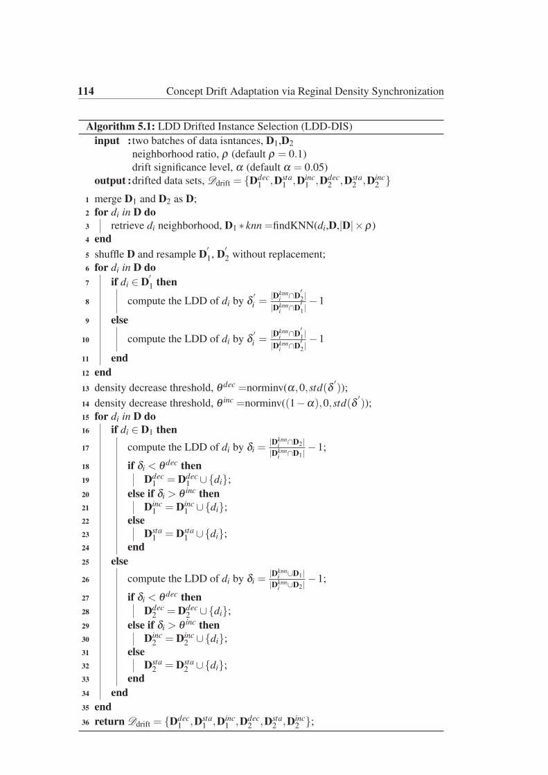
114 Concept Drift Adaptation via Reginal Density Synchronization
Algorithm 5.1: LDD Drifted Instance Selection (LDD-DIS)input : two batches of data isntances, D1,D2
neighborhood ratio, ρ (default ρ = 0.1)drift significance level, α (default α = 0.05)
output :drifted data sets, Ddrift = {Ddec1 ,Dsta
1 ,Dinc1 ,Ddec
2 ,Dsta2 ,Dinc
2 }1 merge D1 and D2 as D;2 for di in D do3 retrieve di neighborhood, D1 ∗ knn =findKNN(di,D,|D|×ρ)4 end5 shuffle D and resample D′
1, D′2 without replacement;
6 for di in D do7 if di ∈ D′
1 then
8 compute the LDD of di by δ ′i =
|Dknni ∩D′
2||Dknn
i ∩D′1|−1
9 else
10 compute the LDD of di by δ ′i =
|Dknni ∩D′
1||Dknn
i ∩D′2|−1
11 end12 end13 density decrease threshold, θ dec =norminv(α,0,std(δ ′
));
14 density decrease threshold, θ inc =norminv((1−α),0,std(δ ′));
15 for di in D do16 if di ∈ D1 then17 compute the LDD of di by δi =
|Dknni ∩D2|
|Dknni ∩D1| −1;
18 if δi < θ dec then19 Ddec
1 = Ddec1 ∪{di};
20 else if δi > θ inc then21 Dinc
1 = Dinc1 ∪{di};
22 else23 Dsta
1 = Dsta1 ∪{di};
24 end25 else26 compute the LDD of di by δi =
|Dknni ∪D1|
|Dknni ∪D2| −1;
27 if δi < θ dec then28 Ddec
2 = Ddec2 ∪{di};
29 else if δi > θ inc then30 Dinc
2 = Dinc2 ∪{di};
31 else32 Dsta
2 = Dsta2 ∪{di};
33 end34 end35 end36 return Ddrift = {Ddec
1 ,Dsta1 ,Dinc
1 ,Ddec2 ,Dsta
2 ,Dinc2 };

5.3 Drifted Instances Selection and Adaptation 115
of LDD when no drift occurs, namely δ ′ ∼ N(μ,σ2), lines 1-13. The second is
to compute LDD for each data instance according to the input data batches, and
selects the drifted instances correspondingly, lines 14-31. Lines 1 to 4 computes the
k-nearest neighbor map of the entire data, where findKNN(di,D, |D|×ρ) stands for
finding the (|D|×ρ) nearest neighbor of di in D. Then, at line 5, we shuffle the data
and resample two new batches D′1, D′
2 with the same size as D1, D2. The resampling
guarantees that D′1 and D′
2 follow an identical distribution. As per theorem 1,
consequently, the δ ′follows 0-mean normal distribution, and the density decreasing
and increasing confidence interval can be calculated by the normal inverse cumulative
distribution function, as shown in lines 12, 13, denoted as norminv(α,0,std(δ ′)),
where α is the significance level, 0 is the mean, and std(δ ′) is the estimated standard
deviation. Then, we compute the LDD for each data instance according to their
original distributions. For each data instance, if its LDD is less than θ dec, it will be
identified as a density decreasing instance, while if its LDD is greater than θ inc, it
will be identified as density increasing instance, as shown in lines 14 to 31. Also, if
the LDD is between θ dec ≤ δi ≤ θ inc, that instance will be considered as a no drift
instance, or a stable instance.
5.3.2 Density synchronized drift adaptation
In this section, a regional drift adaptation algorithm is developed to synchronize
the density discrepancies based on the identified drifted instances. The set Ddec1 ,
which returned by LDD-DIS, represents the data instances belonging to D1 and have
decreased density compared to the set D2. Similarly, the set Dinc2 represents the data
instances belonging to D2 and have increased density compared to data set D1. It is

116 Concept Drift Adaptation via Reginal Density Synchronization
Algorithm 5.2: Density Synchronized Drift Adaptation (LDD-DSDA)input :data instance arriving at each time step d0, . . . ,dt
minimum data batch size, wmin (default wmin = 100)base learner, L (default L: Naive Bayes Classifier)
output :prediction results, y0, . . . , yt
1 initial Dtrain, L =buildLearner(Dtrain);2 while stream not end, denote current time as t do3 yt =predict(L,dt);4 if |Dtrain|< wmin then5 Dtrain = Dtrain∪{dt};6 else7 Dbuffer = Dtrain∪{dt};8 end9 if |Dtrain| ≥ wmin and |Dbuffer| ≥ wmin then
10 D =LDD-DIS(Dtrain,Dbuffer);11 merge the detected drift regions as per Equation 5.9;
12 based on the density of Dbuffer, resample the data as Dtrain, as perEquation 5.10;
13 build new learner, L =buildLearner(Dtrain);14 else15 updateLearner(L,dt);
16 end17 end18 return y0, . . . , yt ;
obvious that, if the size of D1 and D2 are the same, then the size of Ddec1 and Dinc
2
will be the same, or is simply denoted as |Ddec1 |/|D1|= |Dinc
2 |/|D2|. This propertyis the foundation of the proposed LDD-based density synchronized drift adaptation
(LDD-DSDA) in Algorithm 5.2.
The intuitive idea of LDD-DSDA is to merge existing dataDtrain with the recently
buffered data Dbuffer and resample a new batch of training data Dtrain so that the new
Dtrain has the same distribution as Dbuffer. To achieve this goal, we present the fol-
lowing data merging rules: 1) if no density discrepancies are detected (which means

5.3 Drifted Instances Selection and Adaptation 117
|Dd1ec|/|D1|= |Di
2nc|/|D2|= 0) then return Dtrain∪Dbuffer while if the unioned data
set is considered redundant, return Dbuffer instead; 2) if there are regional density
drifts, merging the drifted data instances as per Equation 5.9.
⎧⎪⎪⎪⎪⎪⎪⎨⎪⎪⎪⎪⎪⎪⎩
Dinc = Dinctrain∪Ddec
buffer
Dsta = Dstatrain∪Dsta
buffer
Ddec = Ddectrain∪Dinc
buffer
(5.9)
Then, to ensure the drifted regions have the same probability density as Dbuffer, a
subset of instances in each drifted region will be resampled, denoted as Dsample,
shown as Equation 5.10. where Dincsample are sampled from Ddecin Equation 5.9. and
so on. At last replace Dtrain by Dsample, namely Dtrain = Dsample
|Dincsample| : |Dsta
sample| : |Ddecsample|= |Dinc
buffer| : |Dstabuffer| : |Ddec
buffer| (5.10)
In Algorithm 5.2, line 1 initializes the base learner L, and line 3 uses the base
learner to predict data instances arriving at the current time, denoted as predict(L,dt).
From lines 4 to 7, the system maintains the data for training and drift detection.
When both training and buffered data sets reach the minimum batch size, LDD-DIS
is triggered, as shown in lines 8, 9. Then the detected drift regions are synchronized,
based on Equations 5.9, 5.9. Otherwise, the system incrementally updates the base
learner, denoted as updateLearner(L,dt), shown in line 14. Finally, in line 16, the
predicted labels are returned for performance analysis.

118 Concept Drift Adaptation via Reginal Density Synchronization
5.4 Experiment and Evaluation
In this section, two groups of experiments are conducted to evaluate the proposed
LDD. The first group evaluates the LDD-DIS algorithm. The second group applies
the LDD-DSDA algorithm to three real-world evolving data streams and compare
the results with other methods. All experiments are conducted on a 2×3.1GHz 8core CPU 128GB RAM cluster node with unique access.
5.4.1 Evaluation of LDD-DIS
In this section, the LDD-DIS algorithm is evaluated in terms of two 2D synthetic
drifted datasets. For each dataset, 1,000 training cases are drawn from a specific
distribution and 500 testing cases are drawn from a different distribution. The
estimated probability density curve of the selected feature are plotted in subfigure
(a), the entire dataset are in subfigure (b) (blue dots represent the training set and
red crosses represent the testing set), the detected drifted instances are in subfigure
(c) (blue dots represent decreasing density, red dots represent increasing density),
and the value of LDD of the corresponding instances are in subfigure (d) which
demonstrates the relationship between LDD and regional density changes. The
configurations of LDD are set as the default values described in Algorithm 5.1.
Experiment 5.1. (Gaussian data with drifted variance). This data set is generated
from a bivariate Gaussian distribution. The training set has mean μ = [5,5] and the
covariance matrix is
σ =
⎡⎢⎣1 0
0 1
⎤⎥⎦

5.4 Experiment and Evaluation 119
The testing set has the same mean vector while its covariance matrix drifts to
σ =
⎡⎢⎣3 0
0 3
⎤⎥⎦
This drift forms a ring-shaped drifted region as shown in Figure 5.3(c).
Since the covariance of x1, x2 is 0, the patterns of drifted regions are the same
from only x1 perspective. In Figure 5.3(a), we plot the kernel smoothing estimated
density function of feature x1 for both training set (red line) and testing set (blue
line). If we consider the density drift from the training set perspective, when the blue
line is higher than the red line, this means in that region, the training set density is
decreasing, and vice versa. Accordingly, the instances located in these regions will
be identified as Ddectrain or Dinc
train, as shown in Figure 5.3(c), where the red dots belong
to Dinctrain, and the blue dots belong to Ddec
train. The corresponding LDD value of each
data instance is ploted in Figure 5.3(d). The higher the value of LDD, the higher the
probability that this instance will drift.
Experiment 5.2. (Mixture distribution with drifted mean) To demonstrate how LDD
works in a more general situation, we create a drifting Gaussian mixture data set
and apply LDD to detect the drifted instances. The Gaussian mixture distribution
consists of three bivariate Gaussian distributions. The three distributions for the
testing set are generated based on the paramters given in Equation 5.11, while the
testing set is generated based on the parameters given in Equation 5.12. The results

120 Concept Drift Adaptation via Reginal Density Synchronization
of LDD-DIS are shown in Figure 5.4 with the same interpretation as Figure 5.3.
⎧⎪⎪⎪⎪⎪⎪⎪⎪⎪⎪⎪⎪⎪⎪⎪⎪⎪⎪⎪⎪⎪⎪⎪⎪⎪⎪⎨⎪⎪⎪⎪⎪⎪⎪⎪⎪⎪⎪⎪⎪⎪⎪⎪⎪⎪⎪⎪⎪⎪⎪⎪⎪⎪⎩
μ1 = [8,5],σ1 =
⎡⎢⎢⎣1 0
0 1
⎤⎥⎥⎦
μ2 = [2,5],σ2 =
⎡⎢⎢⎣2 0
0 2
⎤⎥⎥⎦
μ3 = [5,5],σ3 =
⎡⎢⎢⎣5 0
0 5
⎤⎥⎥⎦
(5.11)
⎧⎪⎪⎪⎪⎪⎪⎪⎪⎪⎪⎪⎪⎪⎪⎪⎪⎪⎪⎪⎪⎪⎪⎪⎪⎪⎪⎨⎪⎪⎪⎪⎪⎪⎪⎪⎪⎪⎪⎪⎪⎪⎪⎪⎪⎪⎪⎪⎪⎪⎪⎪⎪⎪⎩
μ1 = [10,5],σ1 =
⎡⎢⎢⎣1 0
0 1
⎤⎥⎥⎦
μ2 = [4,5],σ2 =
⎡⎢⎢⎣2 0
0 2
⎤⎥⎥⎦
μ3 = [7,5],σ3 =
⎡⎢⎢⎣5 0
0 5
⎤⎥⎥⎦
(5.12)

5.4Experim
entandEvaluatio
n121
-5 0 5 10 15x 1
0
0.1
0.2
0.3
0.4
P(X
)
(a) Train Set & Test Set Distirubtion
0 2 4 6 8 10x 1
0
2
4
6
8
10
x 2
(b) Train Set & Test Set
0 2 4 6 8 10x 1
0
2
4
6
8
10
x 2
(c) Drift Instances
2 4 6 8 10x 1
-1
-0.5
0
0.5
1
1.5
LDD
(d) LDD
Figure 5.3 LDD-DIS on Gaussian Distribution with Drifted Variance.
-5 0 5 10 15 20x 1
0
0.05
0.1
0.15
P(X
)
(a) Train Set & Test Set Distirubtion
-2 0 2 4 6 8 10 12x 1
-2
0
2
4
6
8
10
12
x 2
(b) Train Set & Test Set
-2 0 2 4 6 8 10 12x 1
-2
0
2
4
6
8
10
12
x 2
(c) Drift Instances
-5 0 5 10 15x 1
-5
0
5
10
15
LDD
(d) LDD
Figure 5.4 LDD-DIS on Gaussian Mixture Distribution with Drifted Mean.

122 Concept Drift Adaptation via Reginal Density Synchronization
5.4.2 Evaluation of LDD-DSDA
In this section, we evaluate LDD-DSDA on three real-world evolving data streams.
We compare its performance to several representatives of data stream classification
paradigms. The selected comparison methods are: Hoeffding Adaptive Tree (HAT)
Bifet and Gavaldà (2009), AUE1 Brzezinski and Stefanowski (2011), SAMkNN
Losing et al. (2016), ECDD Ross et al. (2012), and HDDM family algorithms
Frias-Blanco et al. (2015). All these algorithms were implemented based on the
MOA framework Bifet et al. (2010a), which is a commonly used software for
evolving data stream analysis. To quantitatively evaluate LDD-DSDA, the following
performance metrics are considered: accuracy (Acc.), precision (Pre.), recall (Rec.),
f1-score (F1.) and computation time (Time), where Pre= T PT P+FP , Rec= T P
T P+FN , and
F1= 2·Pre·RecPre+Rec . The term T P represents the number of true positive predictions, FN
represents the number of false negative predictions. These metrics were evaluated in
a prequential manner. To fairly compare these drift adaptation algorithms, the default
parameters suggested by the authors are used, and the base classification model is
set as Naïve Bayes classifier, except for SAMkNN, which is only designed for IBk
classifier. The parameters for IBk classifier of SAMkNN are k = 10 and weighting
method=uniformly weighted. Because LDD-DSDA involves a random sampling
process, the results may vary at different runs, we run LDD-DSDA 50 times on each
dataset and state the mean and standard deviation of the results. To avoid confusion
on the F1-score metric, we only take the mean of Pre. and Rec. to calculate the F1
for LDD-DSDA. The source code of LDD-DSDA is available online1.
1https://sites.google.com/view/anjin-concept-drift/home

5.4 Experiment and Evaluation 123
Experiment 5.3. (Electricity Price Prediction Dataset) Elec dataset contains 45,312
instances, collected every thirty minutes from the Australian New South Wales
Electricity Market between 7 May 1996 and 5 Dec 1998. In this market, prices are
not fixed and are affected by demand and supply. This dataset contains eight features
and two classes (up, down) and has been widely used for concept drift adaptation
evaluation. We considered the classes as equally important, because both price up
and down in the market is considered critical to users, and the ratio of classes is
balanced, which is 58% down and 42% up. Therefore, we take the average precision
(Pre.) and recall (Rec.) of both classes as the performance evaluation metrics, where
average Pre = (Preclass1+Preclass2)/2, average Rec = (Recclass1+Recclass2)/2.
Experiment 5.4. (Nebraska Weather Prediction Dataset) This dataset was compiled
by the U.S. National Oceanic and Atmospheric Administration. It contains 8 features
and 18,159 instances with 31% positive (rain) class, and 69% negative (no-rain)
class. This dataset was summarized by Polikar and Elwell (2011). In relation to the
performance metrics Pre. Rec. and F1, only the positive class (rain) is considered.
This is because a correct prediction of rain is considered more important than a
correct prediction of no-rain.
Experiment 5.5. (Spam Filtering Dataset) This dataset is a collection of 9,324 email
messages derived from the Spam Assassin collection. The original dataset contains
39,916 features, and 9,324 emails (around 20% spam emails and 80% legitimate
emails). It is commonly considered to be a typical gradual drift dataset Katakis et al.
(2009). According to Katakis et al. (2009), 500 attrib-utes were retrieved using the
chi-square feature selection approach. The correct classification of legitimate emails
is used to evaluate the algorithms Katakis et al. (2009).
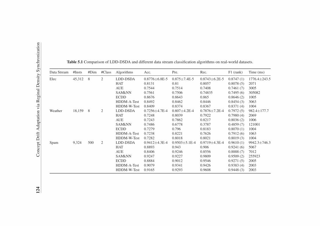
124
ConceptDriftAdaptationviaReginalDensitySynchronization
Table 5.1 Comparison of LDD-DSDA and different data stream classification algorithms on real-world datasets.
Data Stream #Insts #Dim #Class Algorithms Acc. Pre. Rec. F1 (rank) Time (ms)
Elec 45,312 8 2 LDD-DSDA 0.8776±6.8E-5 0.875±7.4E-5 0.8743±6.2E-5 0.8747 (1) 1776.4±243.5HAT 0.8131 0.81 0.8057 0.8078 (5) 2071
AUE 0.7544 0.7514 0.7408 0.7461 (7) 3005
SAMkNN 0.7561 0.7506 0.74835 0.7495 (6) 305082
ECDD 0.8676 0.8643 0.865 0.8646 (2) 1005
HDDM-A-Test 0.8492 0.8462 0.8446 0.8454 (3) 3063
HDDM-W-Test 0.8409 0.8374 0.8367 0.8371 (4) 1004
Weather 18,159 8 2 LDD-DSDA 0.7256±4.7E-4 0.807±4.2E-4 0.7876±7.2E-4 0.7972 (5) 982.4±177.7HAT 0.7248 0.8039 0.7922 0.7980 (4) 2069
AUE 0.7243 0.7862 0.8217 0.8036 (2) 1006
SAMkNN 0.7486 0.6778 0.3787 0.4859 (7) 121001
ECDD 0.7279 0.796 0.8183 0.8070 (1) 1004
HDDM-A-Test 0.7238 0.8221 0.7626 0.7912 (6) 1063
HDDM-W-Test 0.7282 0.8018 0.8021 0.8019 (3) 1004
Spam 9,324 500 2 LDD-DSDA 0.9412±4.3E-4 0.9503±5.1E-4 0.9719±4.3E-4 0.9610 (1) 9942.3±746.3HAT 0.8893 0.943 0.906 0.9241 (6) 5067
AUE 0.8406 0.9246 0.8556 0.8888 (7) 7012
SAMkNN 0.9247 0.9227 0.9809 0.9509 (2) 255923
ECDD 0.8884 0.9012 0.9546 0.9271 (5) 2005
HDDM-A-Test 0.9079 0.9341 0.9426 0.9383 (4) 2003
HDDM-W-Test 0.9165 0.9293 0.9608 0.9448 (3) 2003
5.5 Summary 125
As shown in Table 5.1, LDD-DSDA achieve the best performance in most
cases. Although the execution time of LDD is slightly longer than that of the
other algorithms on high-dimensional data (Experiment 5.5), the improvement is
notable. LDD-DSDA addresses a critical problem in data stream mining from a
novel perspective and achieved a competitive result compared to the state-of-the-art
algorithms. LDD-DSDA has the best average rank (2.33) cross-ing the tested data
sets. Compared to the second place, which is ECDD (2.67), LDD-DSDA improves
the average F1 by 0.0114. According to the Friedman Test, the differences between
LDD-DSDA and ECDD on Acc., Pre., Rec. and F1 are significant.
5.5 Summary
The innovation and main contribution of this chapter is summarized as follow.
Through investigating the distribution of data nearest-neighbors, this chapter pro-
posed a novel metric, called LDD, to detect regional concept drift. Accordingly, an
LDD-based density synchronization algorithm was proposed to adapt the density
discrepancies, called LDD-DSDA. Compared to the other algorithms, LDD-DSDA
addresses drift via density synchronization rather than replacing training data. LDD-
DSDA will not distinguish noise and true data. It would only ensure the adapted
distribution has the same noise distribution and true data distribution as the current
concept. The evaluation results demonstrate that LDD-DSDA accurately identifies
drifted regions and synchronizes the data distribution automatically. Since LDD-
DSDA requires predefined window size, for some real-world scenarios, defining a
nature time window is infeasible, a more flexible regional drift adaptation will be
introduced in the next Chapter.


Chapter 6
Incremental Regional Drift
Adaptation
6.1 Introduction
According to the literature, the objective of existing methods mainly focuses on
identifying the best time to intercept training samples from data streams to construct
the cleanest concept Liu et al. (2017a). Most methods consider concept drift as a
time-related distribution change, or change point, and are disinterested in the spatial
information related to the drift. Without considering the spatial information related
to the drift region, a drift adaptation method can only update learning models or
training sets in terms of time-related information. This may result in unnecessary
reducing the training data Harel et al. (2014). This is especially true if a false alarm
is raised, as incorrect updating the entire training set is costly and may degrade
the overall performance of the learner Alippi et al. (2017); Bu et al. (2016). By
addressing drifts locally, the system will only clean a region if a false alarm is raised

128 Incremental Regional Drift Adaptation
based on spatial (location) information, leaving the other regions unharmed. Thus,
the problem of the training set unnecessarily shrinking can be controlled.
By the same reasoning, a regional drift would not trigger the adaptation until it
becomes globally significant, and would then result in a delay in the drift detection
process. These disadvantages limit the accuracy of learning within evolving data
streams. Therefore, observing a statistically significant change in a local region is
more sensitive than observing a change in the entire feature space because the target
population is different. Assuming that the target population is located in the entire
domain, and a drift only happens in a very small region, the conclusion that there
is no drift in this target population is true. However, such a conclusion may mean
that learning models make the incorrect decision not to update, which would slow
the adaptation process. By contrast, if we set the target population as a set of groups
located in different subdomains, a learning model would make the correct decision
to update the corresponding subdomain no matter which subdomain contains the
drift.
To introduce spatial features into concept drift adaptation, this chapter propose
to divide the concept drift problem into a set of regional density drift problems, as
defined in Chapter 3. The intuition behind the solution is to divide the entire feature
space into a set of sub-feature spaces, then track and adapt to the drifts. Given
concept drift, as a set of regional sudden drifts, can also describe most types of
concept drift, such as sudden drifts, or incremental drifts as discussed Section 3.2.
The novelty and main contribution of this chapter is a novel online regional
drift adaptation algorithm, called online-RDA, that considers drift-related spatial
information to address concept drift problems. Compared to other concept drift
adaptation algorithms, online-RDA demonstrates the following advantages: The

6.2 A Regional Drift Adaptation Framework 129
novelty of this paper is presented in a novel online regional drift adaptation algorithm,
called online-RDA, that considers drift-related spatial information to address concept
drift problems. Compared to other concept drift adaptation algorithms, the online-
RDA demonstrates the following advantages :
1. It is sensitive to regional drift and robust to noise, and drift detection accuracy
is guaranteed by a statistical bound.
2. It tackles concept drift problems locally to control the problem of unnecessarily
shrinking the training data.
3. It is sensitive to regional drifts and can quickly respond to different types of
concept drifts, minimizing the impact caused by drift detection delay.
The rest of this chapter is organized as follows. In Section 6.2, the regional
drift-oriented adaptation framework is introduced. Section 6.3 details the online-
RDA algorithm and presents the implementation pseudocode. Section 6.4 evaluates
online-RDA using various benchmarks, including both artificial streams with known
drift characteristics and highly referenced real-world datasets. Finally, Section 6.5
concludes this study with a discussion of future work.
6.2 A Regional Drift Adaptation Framework
In this section, we propose a general framework for concept drift adaptation oriented
toward regional drift that consists of three stages. The first stage defines and con-
structs the regions. The second stage identifies drifted regions. And the last stage
addresses the drifts in drifted regions. These three stages are shown in Figure 6.1.

130 Incremental Regional Drift Adaptation
If hi has drift
Define Region, h
Convert data sets D as a set of regions
H={h0, …, ht}
For hi in H
Update hi
true
false
Stage 1. Region Construction, D)
Stage 2. Regional Drift Detection,
hi)
Stage 3. Regional Drift Adaptation,
hi)
If hi has drift
Define Region, h
Convert data sets D as a set of regions
H={h0, …, ht}
For hi in H
Update hi
true
false
Stage 1. Region Construction, D)
Stage 2. Regional Drift Detection,
hi)
Stage 3. Regional Drift Adaptation,
hi)Figure 6.1 A concept drift adaptation framework based on regional drift.

6.3 Online Regional Drift Adaptation 131
Stage 1 is constructing the set of regions. Stage 2 exams and highlights the
regions with statistical significant changes. Stage 3 removes or synchronizes the
drifts for each region individually. These three stages are dynamically linked together.
The construction of region set may affect the sensitiveness and the robustness of drift
detection, adaptation process. For example, if a region is too small to include enough
information to conclude the drift within the desired significance level, the detected
drift may have high false alarm. In contrast, if a region is too large, itself may not
be able to capture the drifts within it. Also, the regional drift detection accuracy
will affect the performance of regional drift adaptation. It is critical to optimize the
relationships between region, region drift detection and adaptation to achieve the
best learning results.
For brevity, Stage 1 is denoted as H = Φ(D). In this stage, the dataset D is
converted into a set of regions H. The regional drift detection in Stage 2 is denoted
as Θ(hi), where hi is a region and hi ∈ H\T . The regional drift adaptation in Stage 3
is denoted as Ψ(hi). Stage 3 is discussed in later sections.
6.3 Online Regional Drift Adaptation
In this section, we formally present our concept drift adaptation algorithm – online
regional drift adaptation (online-RDA). Online-RDA has three components as dis-
cussed in Section 6.2. The region construction methodΦ(D) is introduced in Section
6.3.1. The drift detection method Θ(hi) and adaptation method Ψ(hi) is explained
in Sections 6.3.2 and 6.3.3. Finally, the implementation details of learning with
online-RDA are provided in Section 6.3.4.
132 Incremental Regional Drift Adaptation
6.3.1 kNN-based dynamic region construction
The selection of a region construction process directly affects the overall sensi-
tivity of drift detection and adaptation. Setting a certain distance to construct
unit-hyperspheres is one option. However, using a fixed distance may have fewer
drawbacks when dealing with a high-dimensional feature space, arbitrary shapes, and
distributions that have high-density differences within different regions. For example,
sparse unit-hyperspheres may have no data instances while dense unit-hyperspheres
may have too many data instances, which undermines the advantages of regional drift
detection. Similar problems may occur when applying kernel density estimation.
To overcome these problems, we propose using density clustering methods to
construct the regions. According to Tan (2006), density clustering methods group
data instances based on different density, shapes and can perform well under high
dimensional feature space. One of the most intuitive and simple way to construct
a region is using k-nearest neighbours. Given a data instance di and its k-nearest
neighbours, the empirical density can be easily estimated by (k+1)/|D| , where k is
the number of nearest neighbours and |D| is the number of available data instances.The density of the region constructed by di and its k-nearest neighbours can be
easily controlled by selecting the k-value. In other words, given an expected region
density Φ, a dataset can be transformed as a set of regions H = {h0, . . . ,h|D|} thathas P(X ∈ hi) ≈ φ via k = �φ · |D|− 1�. The interval or the radius of region hi is
determined by the distance between data instance di and its furthest neighbour or the
kth nearest neighbour, denoted as:
ε(hi) = maxk∈Z+,k<|D|·φ
(‖di −dk‖) (6.1)
6.3 Online Regional Drift Adaptation 133
In streaming data, the next incoming n data instances, whether or not they are located
in a given region, can be considered as a binomial trail. The set of data instances that
“hit” the same region h from the next continuously arrived n samples is denoted as:
Dhti+1,ti+n = {d j ∈ {dti+1, . . . ,dti+n} : d j ∈ h} (6.2)
If no concept drift occurs during time [0, ti +n], we have
|Dhti+1,n| ∼ B(n, φ) (6.3)
where φ is estimated by φ = |Dh0,ti |/|D0,ti | . In effect, this is the probability that
historical data is located in region h. In a stationary environment, the larger D0,ti is
in size, the more accurate φ will be. According to Box et al. (1978), the distributions
of the count |D| and the sample proportion are approximately normal for largevalues of n. This result follows the central limit theorem. The mean and variance
for an approximately normal distribution of |D| are np and np(1− p), which are
identical to the mean and variance of a B(n, p) distribution. Similarly, the mean and
variance for the approximately normal distribution of the sample proportion are p
and (p(1− p)/n). However, because a normal approximation is not accurate for
small values of n, a good rule of thumb is to use the normal approximation only if
np > 10 and n(1− p)> 10. In other words, we need to constrain |D0,ti | · φ > 10 and
|D0,ti | · (1− φ)> 10 to acquire accurate regions.
To maintain such a region, we only need the center data instance of the region
di, the radius εi, the estimated density φi, and the initialization time ti of the region,
denoted as hi = 〈di,εi, φi, ti〉. However, covering all possible regions or selecting

134 Incremental Regional Drift Adaptation
all possible φ to construct the power region sets H is not practical. Therefore, we
recommend using an ensemble of φ to detect and adapt to concept drifts, namely
allowing φ = {0.05,0.1,0.2}, and using majority voting to finalize the classification,or prediction results.
6.3.2 kNN-based regional drift detection
Constructing the regions is only the first step of the regional drift adaptation frame-
work. The second step is to detect whether any statistical changes have occurred in
a data stream. Therefore, this section introduces a novel kNN-based regional drift
detection and prediction method.
Given a region hi = 〈di,εi, φi, ti〉, the current time is ti + n. The number of
data instances located in region hi are counted during time period [ti + 1, ti + n],
denoted as ui = |Dh jti+1,ti+n|, where Dh j
ti+1,ti+n = {d j ∈ {dti+1, . . . ,dti+n} : ‖di −d j‖<εi}. According to Equation 6.3, the probability of observing such a number ui at
time ti +n can be calculated by
P(|Dh jti+1,ti+n|= ui) = b(ui, ti +n− ti, φi)
= b(ui,n, φi)
(6.4)
where b(k,n, p) is the probability mass function of the binomial distribution, that
b(k,n, p) =(
nk
)pk(1− p)n−k (6.5)

6.3 Online Regional Drift Adaptation 135
Similarly, we can compute the probability of how likely it is that less than ui data
instances are located in region hi, namely the hypothesis test of the regional drift.
P(|Dh jti+1,ti+n| ≤ ui) = F(ui, ti +n− ti, φ)
= F(ui,n, φi)
(6.6)
where F(k,n, p) is the cumulative distribution function of the binomial distribution,
that
F(k,n, p) = P(X ≤ k) = Σ�k�i=0
(ni
)pi(1− p)n−i (6.7)
If P(|Dh jti+1,ti+n| ≤ ui)< α , such an observation has a small probability and a regional
drift is considered to occur in region hi at time ti, where α = 1− pValue guarantees
the false-positive rate. Alternatively, the drift threshold udri f ti can be calculated based
on a binomial inverse cumulative distribution function, that is, if ui ≤ udri f ti then a
regional drift has occurred.
To implement this approach incrementally, we focussed on calculating F(ui =
0,n, ui), which is the probability that there is no other data instance located in region
hi in the next [ti +1, ti +n] period. The current time is denoted as t, then n = t − ti,
and the online regional drift condition can be rewritten as
F(0, t − ti, φi)< α
⇒ Σ�0�j=0
(nj
)φ j
i (1− φi)t−ti− j < α
⇒(
n0
)φ0i (1− φi)
t−ti−0 < α
⇒ (1− φi)t−ti < α
(6.8)
136 Incremental Regional Drift Adaptation
Then, we have Fi+1 = Fi · (1− φi), if ‖di −di+1‖> εi
6.3.3 kNN-based regional drift adaptation
To handle the drifts, the density of drifted regions should be synchronized instead of
being discarded indiscriminately. As explained in the detection method in Section
6.3.2, the probability that a drift has occurred in region hi can be calculated via
F(0, t − ti, φti), which can be used as a weighting method to update the learning
model.
To ensure hi is updated accurately, the learning model will be reinitialized if it
exits a time t, which satisfies the following conditions
t ∈ Z>ti s.t. ‖di −dt‖ ≤ εi and F(0, t − ti, φi)> α (6.9)
This ensures that the radius εti and the estimated density φti become more accurate
as the number of available data increases.
6.3.4 The implementation of online-RDA
In this section, we present the implementation details for online-RDA. The pseu-
docode is provided in Algorithm 1.
The core idea behind online-RDA is to use a buffer to store the regions that are
most relevant to the current concept and to update the learning models regularly
according to the center of the data instances in the stored regions. In Algorithm
6.1 Lines 1-4, the system is initialized based on the training data. Line 5 starts
by processing the streaming data. Line 6 conducts the prediction or classification

6.3 Online Regional Drift Adaptation 137
Algorithm 6.1: online regional drift adaptationinput :data instance arriving at each time step d0, . . . ,dt
k-nearest neighbour ratio, φ (default φ = {0.05,0.1,0.2})base learner, L (default L: IBk Classifier, k = 5, weighting: inverse distance)max buffer size, wmax (default wmax = 1000)
output :prediction results, y0, . . . , yt
1 for φk in φ do2 construct region sets Hk = Φ(Dtrain,φk),H = H ∪{Hk};3 Initial learner lk =buildLearner(Hk → Dk), L = L∪{lk};4 end5 while stream not end, denote current time as t do6 yt =majorityVote(L,dt);7 for Hk in H do8 for hi in Hk do9 if dt ∈ hi then // Equation 6.9
10 reconstruct region hi;
11 else12 if F(0, t − ti, φi)< α then // Equation 6.813 remove hi from Hk;
14 end15 end16 end17 construct region ht , Hk = Hk ∪{ht};18 if |Hk|> wmax then19 Remove hi = min
hi∈HkF(0, t − ti, φi) from Hk;
20 end21 updateLearner(lk,
⋃hi∈Hk
hi → di);
22 end23 end24 return y0, . . . , yt
tasks. The results are returned with the largest weight voted by all learners built with
different k-nearest neighbor ratios φk. Lines 7-22 detect regional drifts and update
the region buffer according to Equations 6.8 and 6.9. Line 17 constructs new regions
as new data is available. Lines 18-20, maintain the buffer size by removing the most
likely drifted regions so that the buffer size does not exceed the maximum limitation.
Line 21 retrieves data instances from the regions stored in the buffer and updates

138 Incremental Regional Drift Adaptation
the learning models accordingly. Lines 23 and 24 detect the end of the stream and
output the prediction or classification results.
In terms of computational complexity, the complexity of the k-nearest neighbor
search can be reduced to O(logn) with a proper data structure, such as kdTree. The
regional drift detection cost for each newly arriving data instance is O(δ logδ ),
where δ ∈ Z+ is a variable that is equal to the current buffer size, and 10φ ≤ δ ≤ wmax.
In addition, the regionsHk that were constructed based on different φk can be updated
separately in a parallel manner, which further reduces the computation time.
6.4 Experiment and Evaluation
This section presents the evaluations of online-RDA on both synthetic and real-world
datasets. Section 6.4.1 aims to demonstrate how online-RDA incrementally detect
and adapt to concept drifts. Section 6.4.2 presents the evaluations with synthetic
datasets of differing noise ratios, followed by Section 6.4.3 with seven real-world
benchmark datasets. The varying of the buffer sizes for different datasets is also
showed in the results, which can be used to investigate the characteristics of drifts in
these datasets.
6.4.1 Evaluation of the capabilities of online-RDA on
drift detection and adaptation
To begin, how well online-RDA can maintain the buffered data instances is evaluated.
This experiment evaluated whether the buffer size changed along with a concept drift
and whether the reserved data instances conveyed information about the most recent

6.4 Experiment and Evaluation 139
Table 6.1 Online-RDA evaluation one-dimensional sudden-incremental drift data generator
Time Period x1 distribution
[t1, t1500] x1 ∼ N(0,1)[t1501, t2500] x1 ∼ N(2,1)[t2501, t3000] x1 ∼ N(2,1−0.0016× (t −2500))[t3001, t4000] x1 ∼ N(2,0.2)
concept. To illustrate how the online adaptation works in the buffer, we used sliding
windows with the same buffer limitation as a contrast. One of the state-of-the-art
drift detection algorithms, HCDTs proposed by Alippi et al. (2017), is also applied
to illustrate why spatial information is important for drift adaptation.
Experiment 6.1. (1D synthetic data with drifted mean and variance) The datasets
were generated from three one-dimensional Gaussian distributions with different
means and variances. The corresponding distributions are given in Table 6.1. For each
time point, one data instance was generated according to the current distribution. To
simulate sudden and incremental drifts, the data distributions were suddenly changed
at t = 1500 and incrementally changed during t = [2501,3000]. The parameters
for HCDTs were set as ICI-based drift detection with a Lepage validation layer
(H-ICI+Lepage), which are the default settings for their program. To maintain the H-
ICI+Lepage data buffer, we applied the most commonly used drift adaptation strategy
Frias-Blanco et al. (2015); Gama et al. (2004), that is, building a new buffer at a
specified warning level and replacing the old buffer at a specified drifting level. The
warning level was set as αwarn = 0.05 and the drifting level was set to αdri f t = 0.01.
Similar to Alippi et al. (2017), we show the experimental results in Figure 6.2.
In general, both H-ICI+Lepage and online-RDA were able to take corrective actions
no matter what types of drift occurred. However, from the buffer size, we can see

140 Incremental Regional Drift Adaptation
that H-ICI+Lepage with warning and drifting levels discarded all historical data
after confirming a sudden drift, even though some of the data may still be useful.
Whereas, online-RDA is capable of trimming irrelevant information from the buffer
and maintaining the historical data that conforms to the current distribution. In
addition, during the incremental drift, H-ICI+Lepage triggered more than one true
positive alarm, which is correct from a drift detection perspective. However, the
available training data in the buffer was overly reduced, which may not be necessary
for drift adaptation. Compared to the sliding window strategy, as shown in the buffer
snapshot at different time points, online-RDA is more sensitive to drift and can
preserve the data instances that convey the information of the most recent concept.
6.4.2 Evaluation of online-RDA on synthetic drift datasets
Synthetic datasets can be used to generate the desired drifting behaviors Gama
et al. (2012); Žliobaite et al. (2014). In this experiment, we applied three data
stream generators based on massive online analysis (MOA) Bifet et al. (2010a)
with common parametrization Bu et al. (2016, 2017); Gomes et al. (2017b); Yu and
Abraham (2017) to evaluate online-RDA. Table 6.2 shows the main characteristics
of the datasets. The selected algorithms were ADWIN-ARF Gomes et al. (2017b),
SAMkNN Losing et al. (2016), HDDM Frias-Blanco et al. (2015), AUE2 Brzezinski
and Stefanowski (2014), kNNWABifet et al. (2013), and ECDD Ross et al. (2012).
We ran all experiments using the MOA software framework, which allows for easy
reproducibility. Since different base classifiers may affect the results Liu et al. (2018),
for SAMkNN, HDDM, kNNWA, and ECDD, the base classifiers were set as IBk,
with 1000 window limits, k = 5, and neighbors were weighted by the inverse of their

6.4 Experiment and Evaluation 141
Figure 6.2 Experiment evaluation of online-RDA on drift detection and adaptation. Subfigure(a-c) show the empirical distributions of the data for three different concepts. Subfigure (d)
presents the data instance arrived at different time for sudden (t = 1500) and incremental(t = [2500,3000]) drifts. Subfigure (e) demonstrates how the buffer size changed under theevolving data streams. The ten snapshots show the data instances stored in buffer at different
time for the dataset with sudden and incremental drifts. For time = 800,2400,4000, thesystem had already recovered from the drifts, therefore, the data instances are almost the
same as the sliding windows’, while for time = 1600,3200, the system was recovering, sothat the buffer size is reduced, and the data instances stored in buffer are different from the
sliding windows’. It also can be seen that the incremental drift changed slower than sudden
drift, so that the number of removed instances from buffer is less than the sudden drift.

142 Incremental Regional Drift Adaptation
Table 6.2 Online-RDA evaluation synthetic data generator
Dataset Drift Type #Instances #Attributes # Class
SEA concepts sudden 10k 3 2
Rotating hyperplane incremental 10k 10 2
Mixed drift mixed 20k 2 4
distance. ADWIN-ARF and AUE2 are decision tree-based algorithms; therefore,
their configurations were set to default in MOA.
Experiment 6.2. (SEA generator) The SEA generator Street and Kim (2001) pro-
duces data streams with three continuous attributes, X = {x1,x2,x3} and x1,x2,x3 ∈[0,10]. An inequality determines the label or class of each data instance, x1+x2 ≤ θ ,
where θ is a threshold to control the decision boundary. The entire data stream
was divided into four concepts of equal size, and the corresponding θ are 8, 9, 7,
9.5. This has been widely used for evaluating sudden drift detection and adaptation
Gomes et al. (2017b); Liu et al. (2017b); Xu and Wang (2017); Yu and Abraham
(2017).
Experiment 6.3. (Hyperplane generator) The rotating hyperplane generator Hulten
et al. (2001) produces data streams with ten continuous attributes, X = {x1, . . . ,x10}and x1, . . . ,x10 ∈ [0,1]. The decision boundary for classification is determined by
Σdi=1wixi ≥ θ , where d is the dimensionality, and wi are weights that randomly
initialize in the range of [0,1]. Incrementally changing the threshold θ produces a
rotating hyperplane decision boundary, thereby, producing incremental concept drifts.
In this experiment we set d = 2, that is, only the first two features had incremental
drifts.

6.4 Experiment and Evaluation 143
Experiment 6.4. (Mixed sudden and incremental drifts) Based on these data gener-
ators, we generated a concept drift dataset with a mixture of drift types. The dataset
was generated by merging the first two features x1,x2 of the hyperplane dataset with
the first two features of the SEA dataset controlled by a random Boolean selector.
If the selector returned true, one SEA data instance was appended to the dataset,
otherwise, the hyperplane data instance was appended. If there was no more SEA
data, we appended all the remaining Hyperplane data, and vice versa. This process
ensured that incremental drifts would not change the order of the sudden drifts. We
also changed the mean of the hyperplane data by x1 = x1−10 so that the hyperplanedata and SEA data did not overlap.
To evaluate how noisy instances might affect drift adaptation algorithms, we
introduced 0%, 5%, 10%, and 15% noise with reversed class labels into each dataset.
To compare the performance of online-RDA with other state-of-the-art concept
drift adaptation algorithms, we ran the algorithms on 50 datasets with the same
configurations and calculated the mean and variance, shown in Table 6.3. The buffer
size is shown in Figure 6.3, as a demonstration of how the data drifted.
6.4.3 Evaluation of online-RDS stream learning on real-world
datasets
To evaluate the ability of online-RDA in addressing real-world problems, we selected
four state-of-the-art concept drift adaptation algorithms and evaluated them with
seven benchmark real-world datasets. The selected algorithms are the same as in
Section 6.4.2. As discussed in Bifet et al. (2015); Gama et al. (2012); Žliobaite et al.
(2015), execution time and memory cost are important in streaming data learning;

144
IncrementalRegionalDriftAdaptation
Table 6.3 The accuracy of online-RDS on synthetic datasets. The final score, in parentheses, was calculated based on the average rank.
Concepts Noise online-RDA SAMkNN ADWIN-RNF AUE2 HDDM-A HDDM-W kNNWA ECDD
SEA 0 97.22±0.13 95.71±0.25 95.44±0.40 91.85±0.14 95.54±0.16 95.08±0.20 94.63±0.28 94.21±0.360.05 92.94±0.17 90.78±0.19 89.83±0.39 87.10±0.20 90.52±0.20 90.35±0.19 89.18±0.33 89.08±0.440.1 88.91±0.13 85.84±0.20 84.97±0.27 82.89±0.23 85.18±0.19 85.22±0.19 84.00±0.26 83.55±0.420.15 85.21±0.18 80.71±0.25 80.21±0.26 78.62±0.23 79.47±0.25 79.49±0.26 78.62±0.29 77.74±0.66
Hyplane 0 92.80±1.66 85.65±2.57 82.06±5.01 86.58±5.21 83.51±2.48 83.64±2.46 80.76±4.35 82.25±2.020.05 89.64±1.34 81.46±2.11 77.89±4.90 82.34±4.99 78.78±2.43 79.15±2.23 76.04±4.07 77.58±1.830.1 86.75±1.04 76.87±2.40 73.22±4.71 78.24±4.61 74.23±2.11 74.32±2.07 71.54±4.02 72.75±1.350.15 84.22±0.74 72.08±1.95 69.18±4.60 74.44±4.02 69.49±2.02 69.63±1.80 67.14±3.70 68.21±1.20
Mix 0 88.62±3.76 82.91±6.58 83.06±6.65 82.32±6.09 82.55±6.62 82.46±6.73 82.58±6.70 80.77±6.560.05 85.71±3.17 79.41±5.99 79.61±5.93 79.25±5.45 78.91±5.98 78.78±6.09 79.02±6.02 77.20±5.730.1 82.86±2.53 75.81±5.37 75.89±5.26 76.00±4.89 74.98±5.30 74.82±5.37 75.10±5.34 73.19±5.010.15 80.22±1.94 72.13±4.80 72.08±4.61 72.72±4.29 70.85±4.57 70.56±4.60 70.96±4.58 69.04±4.25
Average Rank 1 (1) 2.75 (2) 4.42 (3) 4.50 (4) 4.83 (5) 4.92 (6) 6.25 (7) 7.33 (8)

6.4Experim
entandEvaluatio
n145
Figure 6.3 The average buffer size of online-RDA on synthetic datasets. The selected knn ratio, namely the φ , are 0.05,0.1 and 0.2. Theperiod [t1, t2000] is intentionally removed because it contains no special patterns. The first row is the SEA dataset with different noiseratios. It can be seen that SEA concepts have three noticeable spikes, and the spikes are small, medium, and large, which corresponds to
the drift margin changed from |8−9|, |9−7| and |7−9.5|. Although increasing the noise ratio makes the sequence become fuzzy, thedrift patterns can still be captured by online-RDA. The second row is the hyperplane concepts. Because the hyperplane data generator
has no certain variables to control the drift margins, we can only observe the sequence randomly fluctuate. Similar to the SEA concepts,
noise will make the sequence become fuzzy, but the drifts are still observable. The drifts of the mixed concepts are shown in the third
row. However, it is hard to locate the drift patterns. According to these figures, we can see that higher knn ratios are more sensitive to
drifts and will remove more suspicious data instances.
146 Incremental Regional Drift Adaptation
therefore, this information has been provided along with the experimental results.
Table 6.4 summarize the characteristics of the tested datasets, Table 6.5, 6.6, 6.7
show the performance of the tested algorithms. At last, Figure 6.4 shows the changes
of the buffer size of online-RDA.
Experiment 6.5. (Elec dataset) The electricity dataset (Elec). The electricity dataset
contains 45,312 instances, collected every 30 minutes from the Australian New
South Wales Electricity Market between 7 May 1996 and 5 Dec 1998. In this market,
prices are not fixed, but rather they are affected by supply and demand. This dataset
contains eight features and two classes (up, down) and has been widely used to
evaluate concept drift adaptation. The dataset is available from MOA’s website Bifet
et al. (2010a).
Experiment 6.6. (Weather dataset) Nebraska weather prediction dataset (Weather).
The US National Oceanic and Atmospheric Administration compiled this dataset. It
contains eight features and 18,159 instances with 31% positive (rain) class, and 69%
negative (no rain) class. This dataset is summarized in Elwell and Polikar (2011) and
is available at Polikar and Elwell (2011).
Experiment 6.7. (Spam dataset) The spam filtering dataset (Spam). This dataset is
a collection of 9,324 email messages derived from the Spam Assassin collection and
is available online 1. The original dataset contains 39,916 features and 9,324 emails.
It is commonly considered to be a typical gradual drift dataset Katakis et al. (2009).
According to Katakis’s work Katakis et al. (2009), 500 attributes were retrieved
using the Chi-square feature selection approach.
1http://spamassassin.apache.org/

6.4 Experiment and Evaluation 147
Experiment 6.8. (Usenet dataset) The Usenet1 and Usenet2 datasets (Usenet1,
Usenet2). These two datasets were derived from Usenet posts that exist in the 20
Newsgroup collection. The task is to classify messages as either interesting or junk
as they arrive. The dataset is split into five periods. The data in each time period
have different user interest topics. All data instances were concentrated to simulated
sudden/reoccurring drift.
Experiment 6.9. (Airline dataset) The airline dataset (Airline). This dataset consists
of flight arrival and departure details for all commercial flights within the US, from
October 1987 to April 2008. This dataset was originally proposed for regression
problems at the Data Expo competition, 2009. It was subsequently modified by the
MOA team Bifet et al. (2010a) for prediction analysis. Each data instance has seven
features and two classes with 539,388 records in total.
Experiment 6.10. (Covtype dataset) The forest cover type dataset (Covtype). The
task is to predict the type of forest cover from a given observation as determined by
the US Forest Service (USFS) Region 2 resource information system. Each instance
was derived from data originally obtained from the US Geological Survey (USGS)
and USFS data.
From the accuracy and execution efficiency results in Tables 6.5, 6.6, and 6.7, we
conclude that different drift adaptation algorithms are suited for different applications;
there is no perfect algorithm that can achieve the best performance for all datasets.
While the average ranks provided only demonstrate the effectiveness of the algorithm
on the tested datasets, they do provide strong evidence that regional drift detection
and adaptation performed no worse than others in the tested situations, which proves
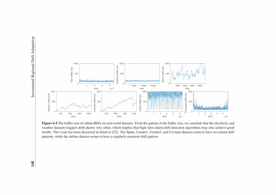
148
IncrementalRegionalDriftAdaptation
1 2 3 4time 10 4
0
500
1000
Ele
c bu
ffer s
ize
5000 10000 15000time
0
500
1000
Wea
ther
buf
fer s
ize
2000 4000 6000 8000time
0
500
1000
Spa
m b
uffe
r siz
e
200 600 1000 1400time
0
500
1000
Use
net1
buf
fer s
ize
200 600 1000 1400time
0
500
1000U
sene
t2 b
uffe
r siz
e
1 2 3 4 5time 10 5
0
500
1000
Airl
ine
buffe
r siz
e
1 2 3 4 5time 10 5
0
500
1000
Cov
erty
pe b
uffe
r siz
e
Figure 6.4 The buffer size of online-RDA on real-world datasets. From the pattern of the buffer size, we conclude that the electricity andweather datasets triggers drift alarms very often, which implies that high false alarm drift detection algorithms may also achieve good
results. This issue has been discussed in detail in [52]. The Spam, Usenet1, Usenet2, and Covtype datasets seem to have no certain drift
patterns, while the airline dataset seems to have a regularly recurrent drift pattern.

6.5 Summary 149
Table 6.4 Online-RDA evaluation real-world dataset characteristics
Dataset #Instances #Attributes #Class
Elec 45312 8 2 (up, down)
Weather 18159 8 2 (rain, no rain)
Spam 9324 500 2 (spam, legitimate)
Usenet1 1500 99 2 (interested, non-interested)
Usenet2 1500 99 2 (interested, non-interested)
Airline 539383 7 2 (delay, not delay)
Covtype 581012 54 7 multiclass
that regional drift adaptation can be an alternative method for addressing concept
drift detection and adaptation problems.
In terms of the algorithm’s efficiency, online-RDA manifested no drawbacks to
execution time. Memory costs were high because online-RDA uses multi-threading,
which consumes more memory. However, this problem can be easily solved via
distributed computing. In addition, the Covtype dataset has more attributes and
data instances than the Airline dataset; however, the execution time for online-RDA,
ADWIN-RNF, and AUE2 on Covtype was much faster. Overall, we conclude that
the execution time of concept drift adaptation algorithms might be related to the
number of drifts in the datasets. In other words, high drift detection accuracy may
result in high execution time. This phenomenon inspired us to reconsider the balance
between drift detection and execution time.
6.5 Summary
The novelty and main contribution of this chapter lies in its aim to divide conventional
concept drift problems into a set of regional drift problems, which can be solved more
easily as a smaller set of individual regional drifts, with the ultimate goal of achieving

150
IncrementalRegionalDriftAdaptation
Table 6.5 Online-RDA evaluation real-world datasets accuracy (%)
Dataset online-RDA ADWIN-RNF SAMkNN HDDM-W kNNWAHDDM-A AUE2 ECDD
Elec 83.08 88.17 82.78 82.47 81.72 82.10 87.74 82.95
Weather 78.21 78.74 77.73 75.04 76.58 76.13 75.24 74.16
Spam 96.30 95.60 95.79 92.93 93.24 92.00 84.29 90.40
Usenet1 68.80 68.40 65.67 69.67 58.33 69.33 63.47 71.60Usenet2 73.00 71.93 71.00 67.93 67.93 68.00 68.87 67.73
Airline 73.49 65.24 60.35 64.54 66.22 65.73 67.51 63.45
Covtype 91.63 92.11 91.71 92.69 93.49 91.17 90.01 88.94
Average Rank 2.43 (1) 2.86 (2) 4.43 (3) 4.93 (4) 4.93 (4) 5.14 (6) 5.14 (6) 6.14 (8)

6.5Summary
151
Table 6.6 Online-RDA evaluation real-world datasets execution time (ms)
Dataset online-RDA ADWIN_RNF SAMkNN HDDM-W kNNWAHDDM-A AUE2 ECDD
Elec 10755 11222 7064 39017 108104 56025 5074 6082
Weather 8273 4005 3004 19008 54023 36018 2004 7005
Spam 15731 6006 23009 1161399 1606493 532170 11007 205070
Usenet1 1300 1003 1002 9005 33008 9005 1003 9006
Usenet2 1131 1005 1002 21013 31011 28015 1002 28013
Airline 1867974 355192 40014 428193 1522319 769335 300139 214094
Covtype 324442 123040 196057 3523827 7167952 2579568 156054 230064
Average Rank 4.71 (5) 2.79 (3) 2.21 (2) 5.93 (6) 7.86 (8) 6.36 (7) 1.86 (1) 4.29 (4)

152
IncrementalRegionalDriftAdaptation
Table 6.7 Online-RDA evaluation real-world datasets memory cost (GB RAM-Hours)
Datasets online-RDA ADWIN-RNF SAMkNN HDDM-W kNNWAHDDM-A AUE2 ECDD
Elec 3.38E-03 1.19E-05 1.36E-05 7.42E-06 2.77E-05 1.05E-05 7.54E-07 1.39E-07Weather 1.35E-03 4.54E-06 4.77E-06 9.63E-07 1.61E-05 7.91E-06 2.00E-07 3.56E-07
Spam 6.95E-04 1.11E-05 1.83E-04 1.03E-02 8.63E-03 4.58E-04 2.28E-05 9.52E-05
Usenet1 1.12E-04 1.43E-07 8.14E-07 3.87E-06 4.39E-05 4.04E-06 5.71E-09 4.07E-06
Usenet2 1.12E-04 1.01E-07 9.59E-07 2.94E-05 4.51E-05 4.50E-05 5.85E-09 4.36E-05
Airline 4.02E-02 5.49E-03 8.41E-05 4.89E-05 4.56E-04 1.57E-04 8.49E-03 3.75E-05Covtype 4.33E-02 1.61E-05 5.64E-04 3.14E-03 8.82E-03 2.31E-03 2.18E-05 1.25E-04
Average Rank 7.71 (8) 3.00 (2) 4.00 (4) 4.29 (5) 6.71 (7) 5.00 (6) 2.29 (1) 3.00 (2)

6.5 Summary 153
a better concept drift adaptation result. To accomplish this aim, a regional drift
adaptation framework is proposed and an online regional drift adaptation algorithm
is developed. The experimental results show that the overall performance of regional
drift adaptation compares to other state-of-the-art algorithms, indicating that regional
drift detection and adaptation has potential as an alternative way of handling concept
drift. In addition, it has been realized that incremental drifts might cause drift
detection algorithms to continually trigger drift alarms, which may be not good for
drift adaptation. Also, the number of drifts in a dataset may contribute to execution
time. Therefore, a compromise may be required to balance execution time with drift
detection and adaptation accuracy.


Chapter 7
Conclusion and Future Research
This chapter concludes the thesis and provides further research directions for this
topic.
7.1 Conclusions
The rapidly changing environment of new products, new markets and new customer
behaviors inevitably results in the appearance of the concept drift problem, which
poses challenges to conventional machine learning assumptions that the training
data and new coming data conform to the same distribution pattern. Stream learning
is the first area to have raised these challenges and now it has spread out to many
other research topics, such as big data mining, active learning, and semi-supervised
learning. Although numerous concept drift detection and adaptation algorithms have
been developed, their research focus is mainly on addressing time-related concept
drift problems. Neither the definition nor the solution has given enough attention to
spatial-related concept drift problems. This thesis theoretically analysed the nature

156 Conclusion and Future Research
of concept drift and proved that concept drift detection and adaptation only based
on time-related information is inadequate and deficient. To improve the accuracy of
drift detection and the effectiveness of drift adaptation, spatial-related information
is introduced to describe concept drift, and a framework to convert conventional
concept drift problems as a set of regional drift problems is developed. The findings
of this study are summarised as follows:
1. The development of a novel regional drift definition to uniformly describe different
types of concept drift, which include both time and spatial information to explain the
nature of concept drift. (To achieve Objective 1)
Regional drift extends the conventional definition of concept drift with drift-
related spatial information. It has been called local drift in other literature, while
no one has given a formal definition to explain the difference and the relationship
between concept drift and local drift. The novelty of regional drift defined in this
study lies in that it uniformly defines concept drift under both discrete and continuous
feature space, as well as describing different types of concept drift as a set of regional
drift. Regional drift provides a theoretical guarantee that addressing the new defined
drift will simultaneously solve the commonly defined drifts.
2. The development of a nearest neighbor-based density variation identification
algorithm (NN-DVI) for regional drift-oriented drift detection. (To achieve Objective
2)
NN-DVI accumulates the density discrepancies of every possible region, and
then examines if the accumulated discrepancy is significant enough to trigger a drift
alarm. NN-DVI consists of data distribution dissimilarity measurement dnnps and a

7.1 Conclusions 157
tailored hypothesis test θ nnps used to determine the critical interval. Compared to
other algorithms, the tailored hypothesis test of NN-DVI proves that dnnps ∼ N(0,σ),
which is the key feature to improve drift detection accuracy while reducing the false
alarm rates. NN-DVI constructs regions based on nearest neighbors which can handle
arbitrary shapes and are friendly to high-dimensionality. NN-DVI demonstrates good
sensitiveness to local drifts as well as to global drifts without sacrificing the false
alarm rate.
3. The development of local drift degree-based density synchronization drift adapta-
tion algorithm (LDD-DSDA) for regional drift-oriented drift adaptation. (To achieve
Objective 3)
The core idea of LDD-DSDA is to detect significant regional density discrepan-
cies and to synchronize these discrepancies based on instance selection. LDD-DSDA
includes a regional density discrepancies measurement, called Local Drift Degree
(LDD), and a drifted data instance selection algorithm, called local drift degree-
based drifted instance selection (LDD-DIS). It is proved that the distribution of LDD
follows a normal distribution. Then, based on these findings, LDD-DIS highlights
suspicious instances, and LDD-DSDA removes or changes the weights of the sus-
picious instance to synchronize the density. LDD-DSDA tries to re-sample useful
data from old concepts, that is, LDD-DSDA is more selective in its action for drift
adaptation, while other drift adaptation algorithms try to remove all data instances
related to old concepts, called the "one-cut" strategy. The experimental results show
that LDD-DSDA can reduce the risk of unnecessary training data shrink, and can
achieve better accuracy than the "one-cut" strategy.

158 Conclusion and Future Research
4. The development of online regional drift adaptation (online-RDA) for incremental
concept drift adaptation. (To achieve Objective 4)
Online-RDA starts with an incremental regional drift adaptation framework
followed by a detailed algorithm that is implemented based on this framework.
The experimental evaluation demonstrates the effectiveness of online-RDA with
limited time and storage constraints and showed several interesting findings, such as
changing of the online-RDA buffer size reflects the drift patterns, which is a note-
worthy study for further research. Online-RDA requests no prior knowledge on the
window size, and has lower computational cost and can be executed on distributed
systems so that the time and storage limitation pose no challenges to the proposed
algorithm.
7.2 Future Study
This thesis identifies the following directions as future work:
• Semi-supervised dri f t detection and adaptation. Current drift detection and
adaptation methods assume that the true label of data instances will be available
after the prediction or classification is made, which implies both the detection
and adaptation process are supervised. However, in real-world scenarios,
the feedback of a prediction or classification, namely the true label, may not
always be available. So, learning how to improve drift detection and adaptation
algorithms for semi or unsupervised circumstances is highly desired.
• Concept-oriented data f iltering. Concept drift problems not only exist in
data stream learning, but are also ubiquitous in train-test batch-based learning,

7.2 Future Study 159
as long as the training and testing data is collected in a time interval rather
than at a time point. For example, in the training and testing data collected in
2017 for customer churn prediction, the available data may include several
concepts. The knowledge patterns may vary in different months or even weeks,
and the most helpful information for customer churn prediction in 2018 may
only be contained in December of 2017. Although the cross-validation strategy
can reduce the overfitting problems of the model build based on the entire
dataset of 2017, it may not be the best solution. Concept drift problems pose
additional challenges to the overfitting and underfitting issues. One possible
solution is concept-oriented data filtering.
• Severity awareness dri f t adaptation. Time and spatial information is im-
portant to identify a drift, which can be considered as two dimensional to
describe concept drift. Another important aspect could be drift severity which
measures and quantifies the significance of a drift. Such information may
further improve the effectiveness of the drift adaptation process for stream
learning.
• Video stream concept dri f t analysis. Since videos are also a type of stream-
ing data, it might possible to apply some of the newly proposed approaches
for video analysis related applications, such as Duan et al. (2012b); Li et al.
(2017a). In addition, the studies related to the connections and the differences
between concept drift adaptation and visual domain adaptation methods Duan
et al. (2012a); Li et al. (2014, 2017b) could also be very useful.

160 Conclusion and Future Research
Handling concept drift is an urgent and important issue. It is a key technique
in achieving adaptive systems. The future research on the adaptivity of machine
learning techniques and systems to concept drift has great prospects.

Bibliography
Aggarwal, C. C., Han, J., Wang, J., and Yu, P. S. (2003). A framework for clustering
evolving data streams. In Proceedings of the Twenty-ninth International Confer-
ence on Very Large Databases, volume 29, pages 81–92. VLDB Endowment.
Ahmadi, Z. and Kramer, S. (2017). Modeling recurring concepts in data streams: a
graph-based framework. Knowledge and Information Systems.
Alippi, C., Boracchi, G., and Roveri, M. (2011). A just-in-time adaptive classification
system based on the intersection of confidence intervals rule. Neural Networks,
24(8):791–800.
Alippi, C., Boracchi, G., and Roveri, M. (2012). Just-in-time ensemble of classifiers.
In Proceedings of rhe 2012 International Joint Conference on Neural Networks,
pages 1–8. IEEE.
Alippi, C., Boracchi, G., and Roveri, M. (2013). Just-in-time classifiers for recur-
rent concepts. IEEE Transactions on Neural Networks and Learning Systems,
162 Bibliography
24(4):620–634.
Alippi, C., Boracchi, G., and Roveri, M. (2017). Hierarchical change-detection tests.
IEEE Transactions on Neural Networks and Learning Systems, 28(2):246–258.
Alippi, C. and Roveri, M. (2008a). Just-in-time adaptive classifiers part i: detecting
nonstationary changes. IEEE Transactions on Neural Networks, 19(7):1145–1153.
Alippi, C. and Roveri, M. (2008b). Just-in-time adaptive classifiers part ii: designing
the classifier. IEEE Transactions on Neural Networks, 19(12):2053–2064.
Andrzejak, A. and Gomes, J. B. (2012). Parallel concept drift detection with online
map-reduce. In Proceedings of the Twelfth IEEE International Conference on
Data Mining Workshops, pages 402–407.
Arabmakki, E. and Kantardzic, M. (2017). Som-based partial labeling of imbalanced
data stream. Neurocomputing, 262:120–133.
Bach, S. H. and Maloof, M. (2008). Paired learners for concept drift. In Proceedings
of the Tenth IEEE International Conference on Data Mining, pages 23–32.
Baena-García, M., del Campo-Ávila, J., Fidalgo, R., Bifet, A., Gavaldà, R., and
Morales-Bueno, R. (2006). Early drift detection method. In Proceedings of the
Fourth International Workshop on Knowledge Discovery from Data Streams, pages
Vol. 6, pp. 77–86.

Bibliography 163
Barddal, J. P., Murilo Gomes, H., Enembreck, F., Pfahringer, B., and Bifet, A. (2016).
On dynamic feature weighting for feature drifting data streams. In Frasconi, P.,
Landwehr, N., Manco, G., and Vreeken, J., editors, Proceedings of the Fourteenth
Joint European Conference on Machine Learning and Knowledge Discovery in
Databases, pages 129–144. Springer.
Basseville, M. and Nikiforov, I. V. (1993). Detection of abrupt changes: theory and
application, volume 104. Prentice Hall Englewood Cliffs.
Bifet, A. and Gavaldà, R. (2007). Learning from time-changing data with adaptive
windowing. In Proceedings of the Seventh SIAM International Conference on
Data Mining, volume 7, page 2007. SIAM.
Bifet, A. and Gavaldà, R. (2009). Adaptive learning from evolving data streams. In
Proceedings of the Eighth International Symposium on Intelligent Data Analysis,
pages 249–260. Springer.
Bifet, A., Holmes, G., Kirkby, R., and Pfahringer, B. (2010a). Moa: massive online
analysis. Journal of Machine Learning Research, 99:1601–1604.
Bifet, A., Holmes, G., and Pfahringer, B. (2010b). Leveraging bagging for evolving
data streams. In Proceedings of the 2010 Joint European Conference on Machine
Learning and Knowledge Discovery in Databases, pages 135–150. Springer.

164 Bibliography
Bifet, A., Holmes, G., Pfahringer, B., and Frank, E. (2010c). Fast perceptron decision
tree learning from evolving data streams. In Zaki, M. J., Yu, J. X., Ravindran,
B., and Pudi, V., editors, Proceedings of the Fourteenth Pacific-Asia Conference
on Knowledge Discovery and Data Mining, pages 299–310. Springer Berlin
Heidelberg.
Bifet, A., Holmes, G., Pfahringer, B., and Gavaldà, R. (2009a). Improving adaptive
bagging methods for evolving data streams. In Zhou, Z.-H. and Washio, T.,
editors, Proceedings of the First Advances in Machine Learning, Lecture Notes in
Computer Science, pages 23–37, Berlin, Heidelberg. Springer Berlin Heidelberg.
Bifet, A., Holmes, G., Pfahringer, B., Kirkby, R., and Gavaldà, R. (2009b). New
ensemble methods for evolving data streams. In Proceedings of the Fifteenth
ACM International Conference on Knowledge Discovery and Data Mining, pages
139–148. ACM.
Bifet, A., Morales, G. d. F., Read, J., Holmes, G., and Pfahringer, B. (2015). Efficient
online evaluation of big data stream classifiers. In Proceedings of the Twenty-first
ACM International Conference on Knowledge Discovery and Data Mining, pages
59–68. ACM.
Bifet, A., Pfahringer, B., Read, J., and Holmes, G. (2013). Efficient data stream
classification via probabilistic adaptive windows. In Proceedings of the Twenty-

Bibliography 165
eighth ACM Symposium on Applied Computing, pages 801–806. ACM.
Blizard, W. D. (1988). Multiset theory. Notre Dame Journal of Formal Logic,
30(1):36–66.
Box, G. E., Hunter, W. G., and Hunter, J. S. (1978). Statistics for experimenters: an
introduction to design, data analysis, and model building, volume 1. JSTOR.
Brzezinski, D. and Stefanowski, J. (2011). Accuracy updated ensemble for data
streams with concept drift. In Proceedings of the 2011 International Conference
on Hybrid Artificial Intelligence Systems, pages 155–163. Springer.
Brzezinski, D. and Stefanowski, J. (2014). Reacting to different types of concept
drift: the accuracy updated ensemble algorithm. IEEE Transactions on Neural
Networks and Learning Systems, 25(1):81–94.
Bu, L., Alippi, C., and Zhao, D. (2016). A pdf-free change detection test based
on density difference estimation. IEEE Transactions on Neural Networks and
Learning Systems, PP(99):1–11.
Bu, L., Zhao, D., and Alippi, C. (2017). An incremental change detection test
based on density difference estimation. IEEE Transactions on Systems, Man, and
Cybernetics: Systems, PP(99):1–13.

166 Bibliography
Cavalcante, R. C., Minku, L. L., and Oliveira, A. L. I. (2016). Fedd: feature
extraction for explicit concept drift detection in time series. In Proceedings of the
2016 International Joint Conference on Neural Networks, pages 740–747.
Cendrowska, J. (1987). Prism: an algorithm for inducing modular rules. International
Journal of Man-Machine Studies, 27(4):349–370.
Chandra, S., Haque, A., Khan, L., and Aggarwal, C. (2016). An adaptive frame-
work for multistream classification. In Proceedings of the Twenty-fifth ACM
International on Conference on Information and Knowledge Management, pages
1181–1190. ACM.
Chu, F. and Zaniolo, C. (2004). Fast and light boosting for adaptive mining of
data streams. In Proceedings of the Eighth Pacific-Asia Advances in Knowledge
Discovery and Data Mining, pages 282–292. Springer Berlin Heidelberg.
Chu, W., Zinkevich, M., Li, L., Thomas, A., and Tseng, B. (2011). Unbiased
online active learning in data streams. In Proceedings of the Seventeenth ACM
International Conference on Knowledge Discovery and Data Mining, pages 195–
203. ACM.
Dasu, T., Krishnan, S., Venkatasubramanian, S., and Yi, K. (2006). An information-
theoretic approach to detecting changes in multi-dimensional data streams. In

Bibliography 167
Proceedings of the Twenty-eighth Symposium on the Interface of Statistics, Com-
puting Science, and Applications, pages 1–24. Citeseer.
Ditzler, G. and Polikar, R. (2011). Semi-supervised learning in nonstationary envi-
ronments. In Proceedings of the 2011 International Joint Conference on Neural
Networks, pages 2741–2748.
Ditzler, G. and Polikar, R. (2013). Incremental learning of concept drift from stream-
ing imbalanced data. IEEE Transactions on Knowledge and Data Engineering,
25(10):2283–2301.
Ditzler, G., Roveri, M., Alippi, C., and Polikar, R. (2015). Learning in nonstationary
environments: a survey. IEEE Computational Intelligence Magazine, 10(4):12–25.
Domingos, P. and Hulten, G. (2000). Mining high-speed data streams. In Proceedings
of the Sixth ACM International Conference on Knowledge Discovery and Data
Mining, pages 71–80. ACM.
Dries, A. and Rückert, U. (2009). Adaptive concept drift detection. Statistical
Analysis and Data Mining: The ASA Data Science Journal, 2(5-6):311–327.
Duan, L., Tsang, I. W., and Xu, D. (2012a). Domain transfer multiple kernel learning.
IEEE Transactions on Pattern Analysis and Machine Intelligence, 34(3):465–479.

168 Bibliography
Duan, L., Xu, D., Tsang, I. W.-H., and Luo, J. (2012b). Visual event recognition in
videos by learning from web data. IEEE Transactions on Pattern Analysis and
Machine Intelligence, 34(9):1667–1680.
Dwass, M. (1957). Modified randomization tests for nonparametric hypotheses. The
Annals of Mathematical Statistics, pages 181–187.
Efron, B. and Tibshirani, R. J. (1994). An introduction to the bootstrap. CRC Press.
Elwell, R. and Polikar, R. (2011). Incremental learning of concept drift in nonsta-
tionary environments. IEEE Transactions on Neural Networks, 22(10):1517–31.
Frías-Blanco, I., Campo-Ávila, J. d., Ramos-Jiménez, G., Carvalho, A. C. P. L. F.,
Ortiz-Díaz, A., and Morales-Bueno, R. (2016). Online adaptive decision trees
based on concentration inequalities. Knowledge-Based Systems, 104:179–194.
Frias-Blanco, I., Campo-Avila, J. d., Ramos-Jimenes, G., Morales-Bueno, R., Ortiz-
Diaz, A., and Caballero-Mota, Y. (2015). Online and non-parametric drift detection
methods based on hoeffding’s bounds. IEEE Transactions on Knowledge and
Data Engineering, 27(3):810–823.
Gama, J. and Castillo, G. (2006). Learning with local drift detection. In Pro-
ceedings of the Second International Conference on Advanced Data Mining and
Applications, pages 42–55. Springer.
Bibliography 169
Gama, J. and Kosina, P. (2013). Recurrent concepts in data streams classification.
Knowledge and Information Systems, 40(3):489–507.
Gama, J., Žliobaite, I., Bifet, A., Pechenizkiy, M., and Bouchachia, A. (2014). A
survey on concept drift adaptation. ACM Computing Surveys, 46(4):1–37.
Gama, J., Medas, P., Castillo, G., and Rodrigues, P. (2004). Learning with drift
detection. In Proceedings of the Seventeenth Brazilian Symposium on Artificial
Intelligence, volume 3171, pages 286–295. Springer.
Gama, J., Rocha, R., and Medas, P. (2003). Accurate decision trees for mining high-
speed data streams. In Proceedings of the Ninth ACM international conference on
Knowledge discovery and data mining, pages 523–528. ACM.
Gama, J., Sebastião, R., and Rodrigues, P. P. (2012). On evaluating stream learning
algorithms. Machine Learning, 90(3):317–346.
Gomes, H. M., Barddal, J. P., Enembreck, F., and Bifet, A. (2017a). A survey
on ensemble learning for data stream classification. ACM Computing Surveys,
50(2):1–36.
Gomes, H. M., Bifet, A., Read, J., Barddal, J. P., Enembreck, F., Pfharinger, B.,
Holmes, G., and Abdessalem, T. (2017b). Adaptive random forests for evolving
data stream classification. Machine Learning.

170 Bibliography
Gomes, J. B., Gaber, M. M., Sousa, P. A., and Menasalvas, E. (2014). Mining
recurring concepts in a dynamic feature space. IEEE Transactions on Neural
Networks and Learning Systems, 25(1):95–110.
Gretton, A., Borgwardt, K. M., Rasch, M. J., Schölkopf, B., and Smola, A. (2012). A
kernel two-sample test. Journal of Machine Learning Research, 13(Mar):723–773.
Gu, F., Zhang, G., Lu, J., and Lin, C.-T. (2016). Concept drift detection based
on equal density estimation. In Proceedings of the 2016 International Joint
Conference on Neural Networks, pages 24–30. IEEE.
Han, D., Giraud-Carrier, C., and Li, S. (2015). Efficient mining of high-speed
uncertain data streams. Applied Intelligence, 43(4):773–785.
Haque, A., Khan, L., and Baron, M. (2016a). Sand: semi-supervised adaptive novel
class detection and classification over data stream. In Proceedings of the Thirtieth
AAAI Conference on Artificial Intelligence, pages 1652–1658.
Haque, A., Khan, L., Baron, M., Thuraisingham, B., and Aggarwal, C. (2016b).
Efficient handling of concept drift and concept evolution over stream data. In
Proceedings of the Thirty-second IEEE International Conference on Data Engi-
neering, pages 481–492.

Bibliography 171
Harel, M., Mannor, S., El-Yaniv, R., and Crammer, K. (2014). Concept drift detection
through resampling. In Proceedings of the Thirty-first International Conference
on Machine Learning, pages 1009–1017.
Heng, W. and Abraham, Z. (2015). Concept drift detection for streaming data.
In Proceedings of the 2015 International Joint Conference on Neural Networks,
pages 1–9.
Hosseini, M. J., Gholipour, A., and Beigy, H. (2015). An ensemble of cluster-
based classifiers for semi-supervised classification of non-stationary data streams.
Knowledge and Information Systems, 46(3):567–597.
Huang, D. T. J., Koh, Y. S., Dobbie, G., and Bifet, A. (2015). Drift detection using
stream volatility. In Appice, A., Rodrigues, P. P., Santos Costa, V., Soares, C.,
Gama, J., and Jorge, A., editors, Proceedings of the Joint European Conference
on Machine Learning and Knowledge Discovery in Databases, pages 417–432.
Springer International Publishing.
Huang, G.-B., Zhu, Q.-Y., and Siew, C.-K. (2006). Extreme learning machine:
Theory and applications. Neurocomputing, 70(1-3):489–501.
Hulten, G., Spencer, L., and Domingos, P. (2001). Mining time-changing data
streams. In Proceedings of the Seventh ACM International Conference on Knowl-
edge Discovery and Data Mining, pages 97–106. ACM.
172 Bibliography
Ikonomovska, E., Gama, J., and Džeroski, S. (2011). Learning model trees from
evolving data streams. Data Mining and Knowledge Discovery, 23(1):128–168.
Ikonomovska, E., Gama, J., and Džeroski, S. (2015). Online tree-based ensembles
and option trees for regression on evolving data streams. Neurocomputing, 150,
Part B(0):458–470.
Ikonomovska, E., Gama, J., Sebastião, R., and Gjorgjevik, D. (2009). Regression
trees from data streams with drift detection. In Gama, J., Costa, V. S., Jorge, A. M.,
and Brazdil, P. B., editors, Proceedings of the Twelfth International Conference
on Discovery Science, pages 121–135, Berlin. Springer.
Katakis, I., Tsoumakas, G., Banos, E., Bassiliades, N., and Vlahavas, I. (2009).
An adaptive personalized news dissemination system. Journal of Intelligent
Information Systems, 32(2):191–212.
Katakis, I., Tsoumakas, G., and Vlahavas, I. P. (2008). An ensemble of classifiers for
coping with recurring contexts in data streams. In Proceedings of the Thirteenth
European Conference on Artificial Intelligence, pages 763–764.
Katal, A., Wazid, M., and Goudar, R. H. (2013). Big data: Issues, challenges, tools
and good practices. In Proceedings of the Sixth International Conference on
Contemporary Computing, pages 404–409.

Bibliography 173
Kawahara, Y. and Sugiyama, M. (2012). Sequential change-point detection based on
direct density-ratio estimation. Statistical Analysis and Data Mining, 5(2):114–
127.
Kifer, D., Ben-David, S., and Gehrke, J. (2004). Detecting change in data streams. In
Proceedings of the Thirtieth International Conference on Very Large Databases,
volume 30, pages 180–191. VLDB Endowment.
Kolter, J. Z. and Maloof, M. A. (2007). Dynamic weighted majority: an ensemble
method for drifting concepts. Journal of Machine Learning Research, 8:2755–
2790.
Kosina, P. and Gama, J. (2015). Very fast decision rules for classification in data
streams. Data Mining and Knowledge Discovery, 29(1):168–202.
Krawczyk, B., Minku, L. L., Gama, J., Stefanowski, J., and Wozniak, M. (2017).
Ensemble learning for data stream analysis: a survey. Information Fusion, 37:132–
156.
Le, T., Stahl, F., Gaber, M. M., Gomes, J. B., and Fatta, G. D. (2017). On expres-
siveness and uncertainty awareness in rule-based classification for data streams.
Neurocomputing, 265:127–141.
Li, P., Wu, X., Hu, X., and Wang, H. (2015). Learning concept-drifting data streams
with random ensemble decision trees. Neurocomputing, 166:68–83.

174 Bibliography
Li, W., Chen, L., Xu, D., and Van Gool, L. (2017a). Visual recognition in rgb images
and videos by learning from rgb-d data. IEEE Transactions on Pattern Analysis
and Machine Intelligence.
Li, W., Duan, L., Xu, D., and Tsang, I. W. (2014). Learning with augmented features
for supervised and semi-supervised heterogeneous domain adaptation. IEEE
Transactions on Pattern Analysis and Machine Intelligence, 36(6):1134–1148.
Li, W., Xu, Z., Xu, D., Dai, D., and Van Gool, L. (2017b). Domain generalization
and adaptation using low rank exemplar svms. IEEE Transactions on Pattern
Analysis and Machine Intelligence.
Žliobaite, I., Bifet, A., Pfahringer, B., and Holmes, G. (2014). Active learning with
drifting streaming data. IEEE Transactions on Neural Networks and Learning
Systems, 25(1):27–39.
Žliobaite, I., Bifet, A., Read, J., Pfahringer, B., and Holmes, G. (2015). Evaluation
methods and decision theory for classification of streaming data with temporal
dependence. Machine Learning, 98(3):455–482.
Žliobaite, I., Pechenizkiy, M., and Gama, J. (2016). An overview of concept drift
applications, book section Chapter 4, pages 91–114. Studies in Big Data. Springer
International Publishing, Cham.

Bibliography 175
Liu, A., Lu, J., Liu, F., and Zhang, G. (2018). Accumulating regional density
dissimilarity for concept drift detection in data streams. Pattern Recognition,
76(Supplement C):256–272.
Liu, A., Song, Y., Zhang, G., and Lu, J. (2017a). Regional concept drift detection
and density synchronized drift adaptation. In Proceedings of the Twenty-sixth In-
ternational Joint Conference on Artificial Intelligence, pages 2280–2286. Accept.
Liu, A., Zhang, G., and Lu, J. (2017b). Fuzzy time windowing for gradual concept
drift adaptation. In Proceedings of the Twenty-sixth IEEE International Conference
on Fuzzy Systems. IEEE.
Liu, A., Zhang, G., Lu, J., Lu, N., and Lin, C.-T. (2016a). An online competence-
based concept drift detection algorithm. In Proceedings of the 2016 Australasian
Joint Conference on Artificial Intelligence, pages 416–428. Springer.
Liu, D., Wu, Y., and Jiang, H. (2016b). Fp-elm: an online sequential learning
algorithm for dealing with concept drift. Neurocomputing, 207:322–334.
Losing, V., Hammer, B., and Wersing, H. (2016). Knn classifier with self adjusting
memory for heterogeneous concept drift. In Proceedings of the Sixteenth IEEE
International Conference on Data Mining, pages 291–300.
Lu, N., Lu, J., Zhang, G., and De Mantaras, R. L. (2016). A concept drift-tolerant
case-base editing technique. Artificial Intelligence, 230:108–133.

176 Bibliography
Lu, N., Zhang, G., and Lu, J. (2014). Concept drift detection via competence models.
Artificial Intelligence, 209:11–28.
Manly, B. F. J. and Mackenzie, D. (2000). A cumulative sum type of method for
environmental monitoring. Environmetrics, 11(2):151–166.
Minku, L. L., White, A. P., and Yao, X. (2010). The impact of diversity on online en-
semble learning in the presence of concept drift. IEEE Transactions on Knowledge
and Data Engineering, 22(5):730–742.
Mirza, B. and Lin, Z. (2016). Meta-cognitive online sequential extreme learning
machine for imbalanced and concept-drifting data classification. Neural Networks,
80:79–94.
Mirza, B., Lin, Z., and Liu, N. (2015). Ensemble of subset online sequential extreme
learning machine for class imbalance and concept drift. Neurocomputing, 149:316–
329.
Morales, G. D. F., Bifet, A., Khan, L., Gama, J., and Fan, W. (2016). Iot big
data stream mining. In Proceedings of the Twenty-second ACM International
Conference on Knowledge Discovery and Data Mining, pages 2119–2120. ACM.
Moreno-Torres, J. G., Raeder, T., Alaiz-Rodríguez, R., Chawla, N. V., and Herrera,
F. (2012). A unifying view on dataset shift in classification. Pattern Recognition,
45(1):521–530.

Bibliography 177
Nguyen, V., Nguyen, T. D., Le, T., Venkatesh, S., and Phung, D. (2016). One-
pass logistic regression for label-drift and large-scale classification on distributed
systems. In Proceedings of the Sixteenth IEEE International Conference on Data
Mining, pages 1113–1118.
Nishida, K. and Yamauchi, K. (2007). Detecting concept drift using statistical
testing. In Corruble, V., Takeda, M., and Suzuki, E., editors, Proceedings of the
Tenth International Conference on Discovery Science, pages 264–269, Berlin,
Heidelberg. Springer Berlin Heidelberg.
Opdyke, J. (2003). Fast permutation tests that maximize power under conventional
monte carlo sampling for pairwise and multiple comparisons. Journal of Modern
Applied Statistical Methods, 2(1):5.
Oza, N. C. and Russell, S. (2001). Experimental comparisons of online and batch
versions of bagging and boosting. In Proceedings of the Seventh ACM Interna-
tional Conference on Knowledge Discovery and Data Mining, pages 359–364,
502565. ACM.
Pietruczuk, L., Rutkowski, L., Jaworski, M., and Duda, P. (2016). A method for
automatic adjustment of ensemble size in stream data mining. In Proceedings of
the 2016 International Joint Conference on Neural Networks, pages 9–15.

178 Bibliography
Polikar, R. and Elwell, R. (2011). Benchmark datasets for evaluating concept drift
nse algorithms. In Editor, editor, Conference Name, volume Volume, page Pages,
[Online] http://users.rowan.edu/ polikar/research/NSE. Publisher.
Pratama, M., Anavatti, S. G., Joo, M., and Lughofer, E. D. (2015). pclass: an
effective classifier for streaming examples. IEEE Transactions on Fuzzy Systems,
23(2):369–386.
Pratama, M., Lu, J., Lughofer, E., Zhang, G., and Anavatti, S. (2016). Scaffolding
type-2 classifier for incremental learning under concept drifts. Neurocomputing,
191:304–329.
Ramírez-Gallego, S., Krawczyk, B., García, S., Wozniak, M., and Herrera, F. (2017).
A survey on data preprocessing for data stream mining: Current status and future
directions. Neurocomputing, 239:39–57.
Raza, H., Prasad, G., and Li, Y. (2015). Ewma model based shift-detection methods
for detecting covariate shifts in non-stationary environments. Pattern Recognition,
48(3):659–669.
Ross, G. J., Adams, N. M., Tasoulis, D. K., and Hand, D. J. (2012). Exponentially
weighted moving average charts for detecting concept drift. Pattern Recognition
Letters, 33(2):191–198.

Bibliography 179
Rutkowski, L., Jaworski, M., Pietruczuk, L., and Duda, P. (2014). Decision trees for
mining data streams based on the gaussian approximation. IEEE Transactions on
Knowledge and Data Engineering, 26(1):108–119.
Rutkowski, L., Jaworski, M., Pietruczuk, L., and Duda, P. (2015). A new method for
data stream mining based on the misclassification error. IEEE Transactions on
Neural Networks and Learning Systems, 26(5):1048–1059.
Rutkowski, L., Pietruczuk, L., Duda, P., and Jaworski, M. (2013). Decision trees
for mining data streams based on the mcdiarmid’s bound. IEEE Transactions on
Knowledge and Data Engineering, 25(6):1272–1279.
Sarnelle, J., Sanchez, A., Capo, R., Haas, J., and Polikar, R. (2015). Quantifying
the limited and gradual concept drift assumption. In Proceedings of the 2015
International Joint Conference on Neural Networks, pages 1–8.
Schlimmer, J. C. and Granger Jr, R. H. (1986). Incremental learning from noisy data.
Machine Learning, 1(3):317–354.
Shao, J., Ahmadi, Z., and Kramer, S. (2014). Prototype-based learning on concept-
drifting data streams. In Proceedings of the Twentieth ACM International Con-
ference on Knowledge Discovery and Data Mining, pages 412–421, 2623609.
ACM.

180 Bibliography
Silva, J. A., Faria, E. R., Barros, R. C., Hruschka, E. R., de Carvalho, A. C., and
Gama, J. (2013). Data stream clustering: A survey. ACM Computing Surveys,
46(1):1–31.
Soares, S. G. and Araújo, R. (2016). An adaptive ensemble of on-line extreme
learning machines with variable forgetting factor for dynamic system prediction.
Neurocomputing, 171:693–707.
Song, X., He, H., Niu, S., and Gao, J. (2016). A data streams analysis strategy based
on hoeffding tree with concept drift on hadoop system. In Proceedings of the
Fourth International Conference on Advanced Cloud and Big Data, pages 45–48.
Song, X., Wu, M., Jermaine, C., and Ranka, S. (2007). Statistical change detection
for multi-dimensional data. In Proceedings of the Thirteenth ACM International
Conference on Knowledge Discovery and Data Mining, pages 667–676, 1281264.
ACM.
Sousa, M. R., Gama, J., and Brandão, E. (2016). A new dynamic modeling framework
for credit risk assessment. Expert Systems with Applications, 45:341–351.
Stoica, I., Song, D., Popa, R. A., Patterson, D. A., Mahoney, M. W., Katz, R. H.,
Joseph, A. D., Jordan, M., Hellerstein, J. M., Gonzalez, J., Goldberg, K., Ghodsi,
A., Culler, D. E., and Abbeel, P. (2017). A berkeley view of systems challenges
Bibliography 181
for ai. Report UCB/EECS-2017-159, EECS Department, University of California,
Berkeley.
Storkey, A. (2009). When training and test sets are different: characterizing learning
transfer. Dataset Shift in Machine Learning, pages 3–28.
Street, W. N. and Kim, Y. (2001). A streaming ensemble algorithm (sea) for large-
scale classification. In Proceedings of the Seventh ACM International Conference
on Knowledge Discovery and Data Mining, pages 377–382, 502568. ACM.
Sun, Y., Tang, K., Minku, L. L., Wang, S., and Yao, X. (2016). Online ensemble
learning of data streams with gradually evolved classes. IEEE Transactions on
Knowledge and Data Engineering, 28(6):1532–1545.
Tan, P.-N. (2006). Introduction to data mining. Pearson Education India.
Tennant, M., Stahl, F., Rana, O., and Gomes, J. B. (2017). Scalable real-time
classification of data streams with concept drift. Future Generation Computer
Systems, 75:187–199.
Tsymbal, A. (2004). The problem of concept drift: definitions and related work.
Thesis, School of Computer Science and Statistics, Computer Science Department,
Trinity College Dublin.

182 Bibliography
Wang, S., Minku, L. L., Ghezzi, D., Caltabiano, D., Tino, P., and Yao, X. (2013).
Concept drift detection for online class imbalance learning. In Proceedings of the
2013 International Joint Conference on Neural Networks, pages 1–10.
Wang, S., Minku, L. L., and Yao, X. (2015). Resampling-based ensemble methods
for online class imbalance learning. IEEE Transactions on Knowledge and Data
Engineering, 27(5):1356–1368.
Wang, S., Minku, L. L., and Yao, X. (2018). A systematic study of online class
imbalance learning with concept drift. IEEE Transactions on Neural Networks
and Learning Systems.
Widmer, G. and Kubat, M. (1996). Learning in the presence of concept drift and
hidden contexts. Machine Learning, 23(1):69–101.
Wu, X., Li, P., and Hu, X. (2012). Learning from concept drifting data streams with
unlabeled data. Neurocomputing, 92:145–155.
Xu, S. and Wang, J. (2017). Dynamic extreme learning machine for data stream
classification. Neurocomputing, 238:433–449.
Xu, Y., Xu, R., Yan, W., and Ardis, P. (2017). Concept drift learning with alternating
learners. In Proceedings of the 2017 International Joint Conference on Neural
Networks, pages 2104–2111.

Bibliography 183
Yamada, M., Kimura, A., Naya, F., and Sawada, H. (2013). Change-point detection
with feature selection in high-dimensional time-series data. In Proceedings of
the Twenty-Third International Joint Conference on Artificial Intelligence, pages
1827–1833.
Yang, H. and Fong, S. (2012). Incrementally optimized decision tree for noisy big
data. In Proceedings of the First International Workshop on Big Data, Streams
and Heterogeneous Source Mining Algorithms, Systems, Programming Models
and Applications, pages 36–44, 2351322. ACM.
Yang, H. and Fong, S. (2015). Countering the concept-drift problems in big data
by an incrementally optimized stream mining model. Journal of Systems and
Software, 102:158–166.
Yeh, Y.-R. and Wang, Y.-C. F. (2013). A rank-one update method for least squares
linear discriminant analysis with concept drift. Pattern Recognition, 46(5):1267–
1276.
Yin, X.-C., Huang, K., and Hao, H.-W. (2015). De2: dynamic ensemble of ensembles
for learning nonstationary data. Neurocomputing, 165:14–22.
You, S.-C. and Lin, H.-T. (2016). A simple unlearning framework for online learning
under concept drifts. In Proceedings of the Twenty-first Pacific-Asia Conference
on Knowledge Discovery and Data Mining, pages 115–126. Springer.

184 Bibliography
Yu, S. and Abraham, Z. (2017). Concept drift detection with hierarchical hypothesis
testing. In Proceedings of the Seventeenth SIAM International Conference on
Data Mining, pages 768–776. SIAM.
Zhang, P., Li, J., Wang, P., Gao, B. J., Zhu, X., and Guo, L. (2011). Enabling fast
prediction for ensemble models on data streams. In Proceedings of the Seventeenth
ACM International Conference on Knowledge Discovery and Data Mining, pages
177–185. ACM.
Zhang, P., Zhu, X., and Shi, Y. (2008). Categorizing and mining concept drifting
data streams. In Proceedings of the Fourteenth ACM International Conference on
Knowledge Discovery and Data Mining, pages 812–820. ACM.
Zhang, P., Zhu, X., Tan, J., and Guo, L. (2010). Classifier and cluster ensembles
for mining concept drifting data streams. In Proceedings of the Tenth IEEE
International Conference on Data Mining, pages 1175–1180.
Zhang, Y., Chu, G., Li, P., Hu, X., and Wu, X. (2017). Three-layer concept drifting
detection in text data streams. Neurocomputing, 260:393–403.
Appendix
List of Abbreviations
ADWIN ADaptive WINdowing pp. 31, 37, 43
ARF Adaptive Random Fores p. 43
ASL achieved significance level pp. 73, 88
AUE Accuracy Update Ensemble pp. 45, 120
CDF cumulative distribution function p. 47
CI-CUSUM Computational Intelligence-based CUSUM test p. 34
CM CompetenceModel-based drift detection pp. 34, 37, 81, 89
CUSUM CUmulative SUM pp. 34, 40
CVFDT Concept-adapting Very Fast Decision Tree pp. 7, 41, 42
DDM Drift Detection Method pp. 22, 29, 31, 37
DELM Dynamic Extreme Learning Machine pp. 29, 37, 39
DWM Dynamic Weighted Majority p. 44
ECDD EWMA for Concept Drift Detection pp. 29, 37, 120, 123
EDDM Early Drift Detection Method pp. 29, 37
EDE Equal Density Estimation pp. 34, 37
ELM Extreme Learning Machine pp. 29, 39

186 Appendix
ESOS-ELM Ensemble of Subset Online Sequential Extreme Learning
Machine p. 21
EWMA Exponentially Weighted Moving Average p. 29
FEDD Feature Extraction for explicit concept Drift Detection
p. 24
FN false negative p. 35
FP false positive pp. 5, 35
FP-ELM Forgetting Parameters Extreme Learning Machine p. 39
FW-DDM Fuzzy Windowing Drift Detection Method pp. 29, 37
HAT Hoeffding Adaptive Tree p. 120
HCDTs Hierarchical Change-Detection Tests pp. 36, 37
HDDM Heoffding’s inequality based Drift Detection Method
pp. 29, 37, 120
HLFR Hierarchical Linear-Four Rate p. 37
IoT Internet of Things pp. 1, 26
IV Information Value p. 36
IV-Jac Information Value and Jaccard similarity p. 36
JIT Just-In-Time adaptive classifiers pp. 34, 37
kNN k-Nearest Neighbor pp. 40, 113
KS Kolmogorov-Smirnov test p. 80
LCM lowest common multiple p. 64
LDD Local Drift Degree pp. 13, 108, 110, 113, 117, 118, 125
LDD-DIS LocalDriftDegree-basedDrifted Instance Selection pp. 13,
113, 115, 117, 118

List of Abbreviations 187
LDD-DSDA Local Drift Degree-based Density Synchronization Drift
Adaptation pp. viii, 10, 13, 34, 37, 115–117, 120, 123, 125
Learn++.CDS Learn++ for Concept Drift with SMOTE p. 21
Learn++.NIE Learn++ for Non-stationary and Imbalanced
Environments p. 21
Learn++.NSE Learn++ for Non-Stationary Environment pp. 21, 44
LFR Linear Four Rate drift detection pp. 35, 37
LLDD Learning with Local Drift Detection pp. 29, 37
LSDD-CDT Least Squares Density Difference-based Change Detection
Test pp. 34, 37
LSLDA Least Squares Linear Discovery Analysis p. 24
LVGB LeVeraGing Bagging p. 43
MC-NN Micro-Cluster Nearest Neighbor p. 22
MMD Maximum Mean Discrepancy p. 88
NEFCS Noise-Enhanced Fast Context Switch p. 40
NN-DVI Nearest Neighbor-based Density Variation Identification
pp. viii, 9, 13, 54, 55, 76, 81, 82, 88, 89
NNPS Nearest Neighbor-based Partitioning Schema pp. 60, 62,
63, 66, 67, 69, 77
OMR-DDM Online Map-Reduce Drift Detection Method p. 22
online-RDA online Regional Drift Adaptation pp. viii, 10, 13, 129
OOB Oversampling-based Online Bagging p. 21
OS-ELM Online Sequential Extreme Learning Machine pp. 21, 39
OWA Optimal Weights Adjustment p. 45

188 Appendix
PCA principal component analysis p. 34
PDF probability density function p. 47
RD Relativized Discrepancy pp. 33, 37
RDA Regional Drift Adaptation pp. viii, 13
SAMkNN Self Adjusting Memory kNN pp. 39, 120
SAND Semi-supervised Adaptive Novel class Detection p. 23
SMOTE Synthetic Minority class Oversampling TEchnique p. 21
SRR Stepwise Redundancy Removal p. 40
STEPD Statistical Test of Equal Proportions Detection pp. 31, 37
TN true negative p. 35
TP true positive pp. 5, 35
TSMSD-EWMA Two-Stage Multivariate Shift-Detection based on EWMA
p. 37
UOB Undersampling-based Online Bagging p. 21
VFDR Very Fast Decision Rules p. 24
VFDT Very Fast Decision Tree pp. 41, 42
VFDTc VFDT deal with continuous data p. 41
WoE Weight of Evidence p. 36