CONCENTRATIONS OF SELECTED ANALYTES IN RURAL NEW …

APPENDIX D

CONCENTRATIONS OF SELECTED ANALYTES IN RURAL NEW YORK STATE SURFACE SOILS: A SUMMARY REPORT ON

THE STATEWIDE RURAL SURFACE SOIL SURVEY

AUGUST 2005

CONTENTS

Summary ............................................................................................................ 5 Introduction ......................................................................................................... 7 A. Project Design Purpose of the Statewide Survey ............................................................. 9 Definitions ................................................................................................. 9 Number of Samples Collected ................................................................ 10 Sample Site Selection ............................................................................. 12 Sample Collection and Transport ............................................................ 15 Laboratory Analysis & Data Reporting .................................................... 15 Assignment of Soil Order and Suborder ................................................. 16 B. Data Analysis Methods Assessment of Data Quality ..................................................................... 18 Distribution of Sampling Locations .......................................................... 18

Descriptive Statistics ............................................................................... 18 C. Results

Assessment of Data Quality ..................................................................... 20 Distribution of Sampling Locations .......................................................... 22

Descriptive Statistics ............................................................................... 22

LIST OF FIGURES

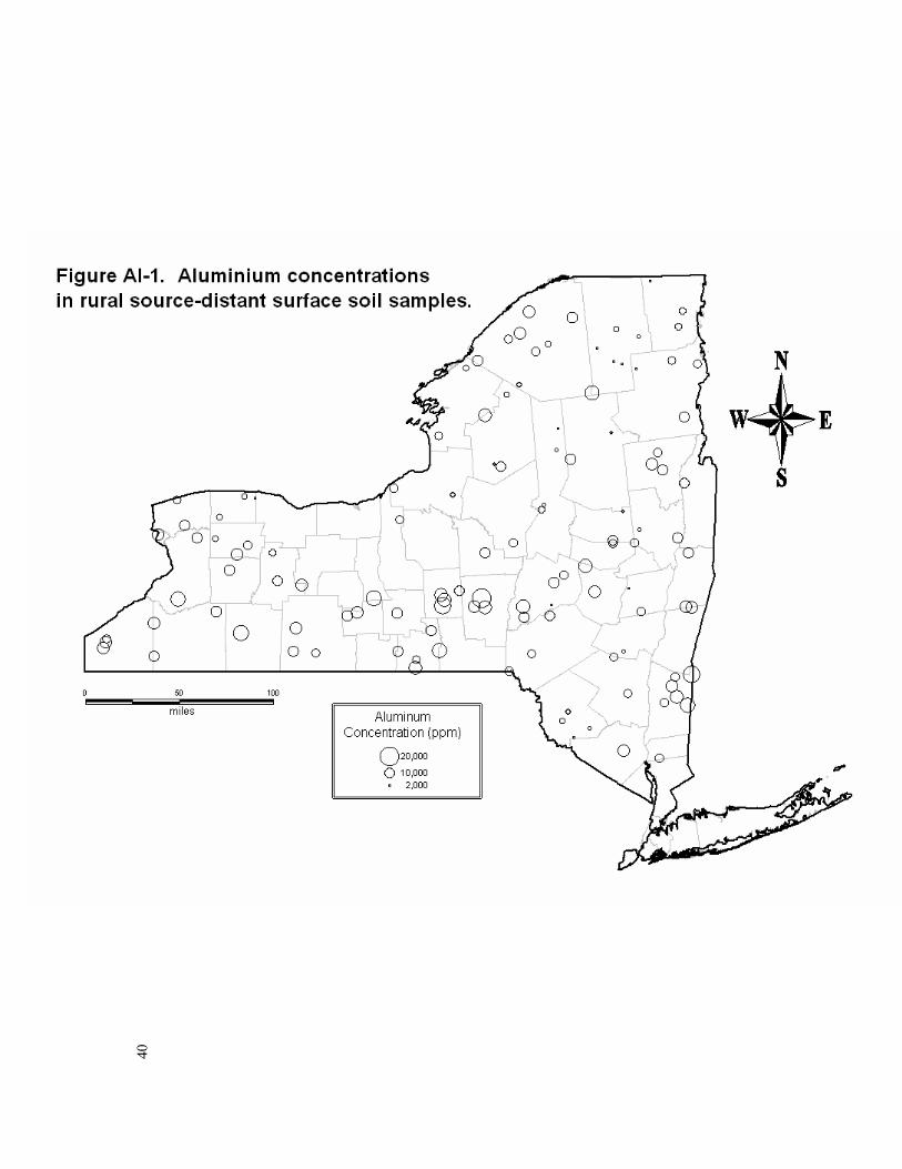
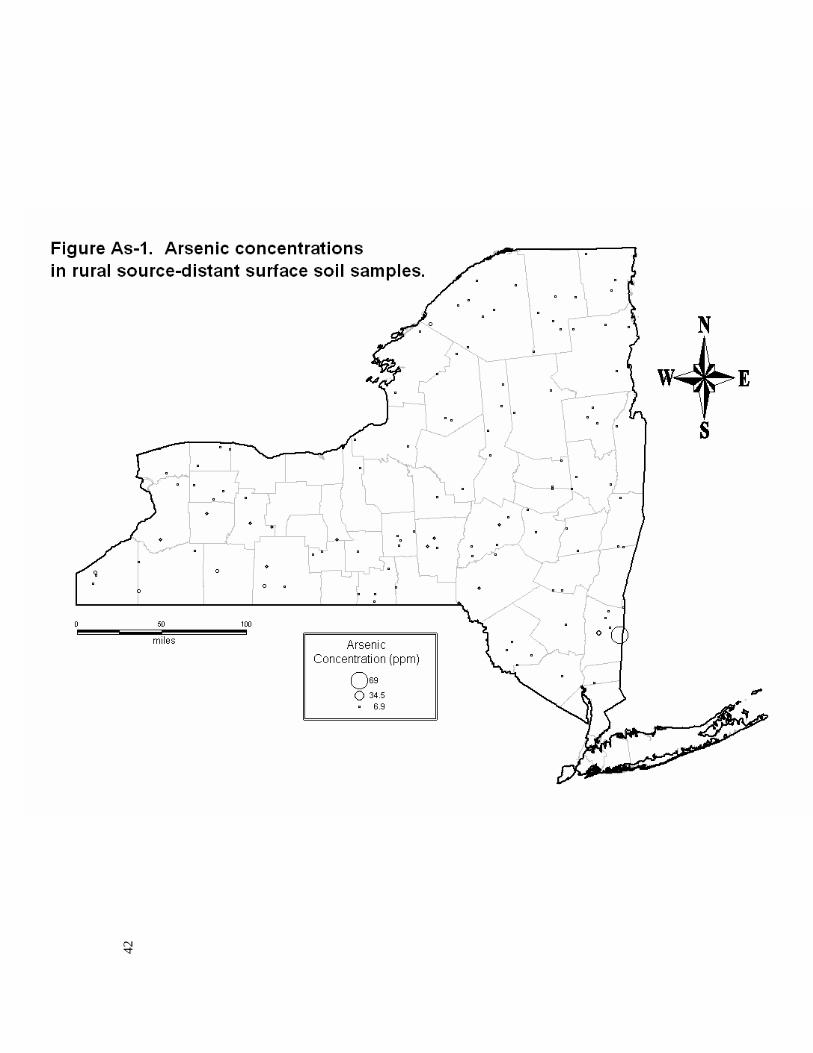
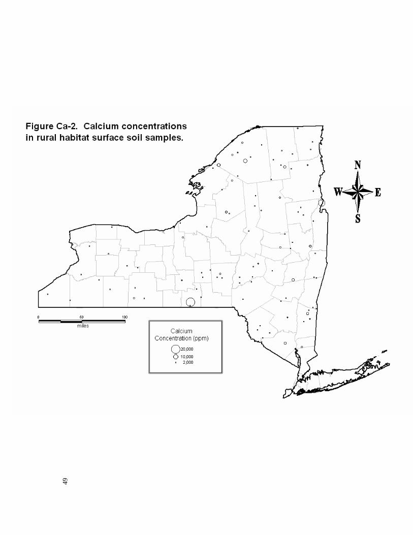
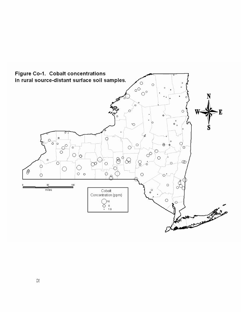
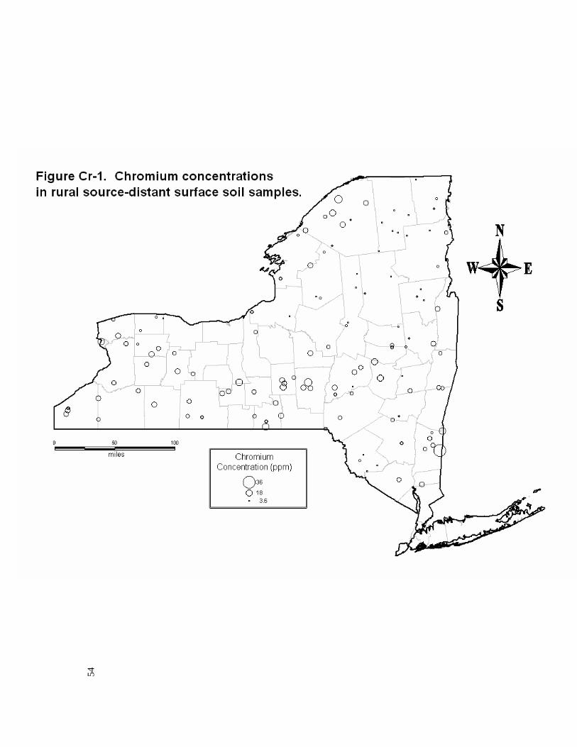
Figure 1: Soil Orders of New York State Figure 2: Source-Distant Surface Soil Sampling Locations Figure 3: Habitat Area Surface Soil Sampling Locations Figure 4: Near Source Surface Soil Sampling Locations Figure Ag-1: Statewide Silver Concentration Map (Source-Distant) Figure Ag-2: Statewide Silver Concentration Map (Habitat) Figure Al-1: Statewide Aluminum Concentration Map (Source-Distant) Figure Al-2: Statewide Aluminum Concentration Map (Habitat) Figure As-1: Statewide Arsenic Concentration Map (Source-Distant) Figure As-2: Statewide Arsenic Concentration Map (Habitat) Figure Ba-1: Statewide Barium Concentration Map (Source-Distant) Figure Ba-2: Statewide Barium Concentration Map (Habitat) Figure Be-1: Statewide Beryllium Concentration Map (Source-Distant) Figure Be-2: Statewide Beryllium Concentration Map (Habitat) Figure Ca-1: Statewide Calcium Concentration Map (Source-Distant) Figure Ca-2: Statewide Calcium Concentration Map (Habitat) Figure Cd-1: Statewide Cadmium Concentration Map (Source-Distant) Figure Cd-2: Statewide Cadmium Concentration Map (Habitat) Figure Co-1: Statewide Cobalt Concentration Map (Source-Distant) Figure Co-2: Statewide Cobalt Concentration Map (Habitat) Figure Cr-1: Statewide Chromium Concentration Map (Source-Distant) Figure Cr-2: Statewide Chromium Concentration Map (Habitat) Figure Cu-1: Statewide Copper Concentration Map (Source-Distant) Figure Cu-2: Statewide Copper Concentration Map (Habitat) Figure Fe-1: Statewide Iron Concentration Map (Source-Distant) Figure Fe-2: Statewide Iron Concentration Map (Habitat) Figure Hg-1: Statewide Mercury Concentration Map (Source-Distant) Figure Hg-2: Statewide Mercury Concentration Map (Habitat) Figure K-1: Statewide Potassium Concentration Map (Source-Distant) Figure K-2: Statewide Potassium Concentration Map (Habitat) Figure Mn-1: Statewide Manganese Concentration Map (Source-Distant) Figure Mn-2: Statewide Manganese Concentration Map (Habitat)

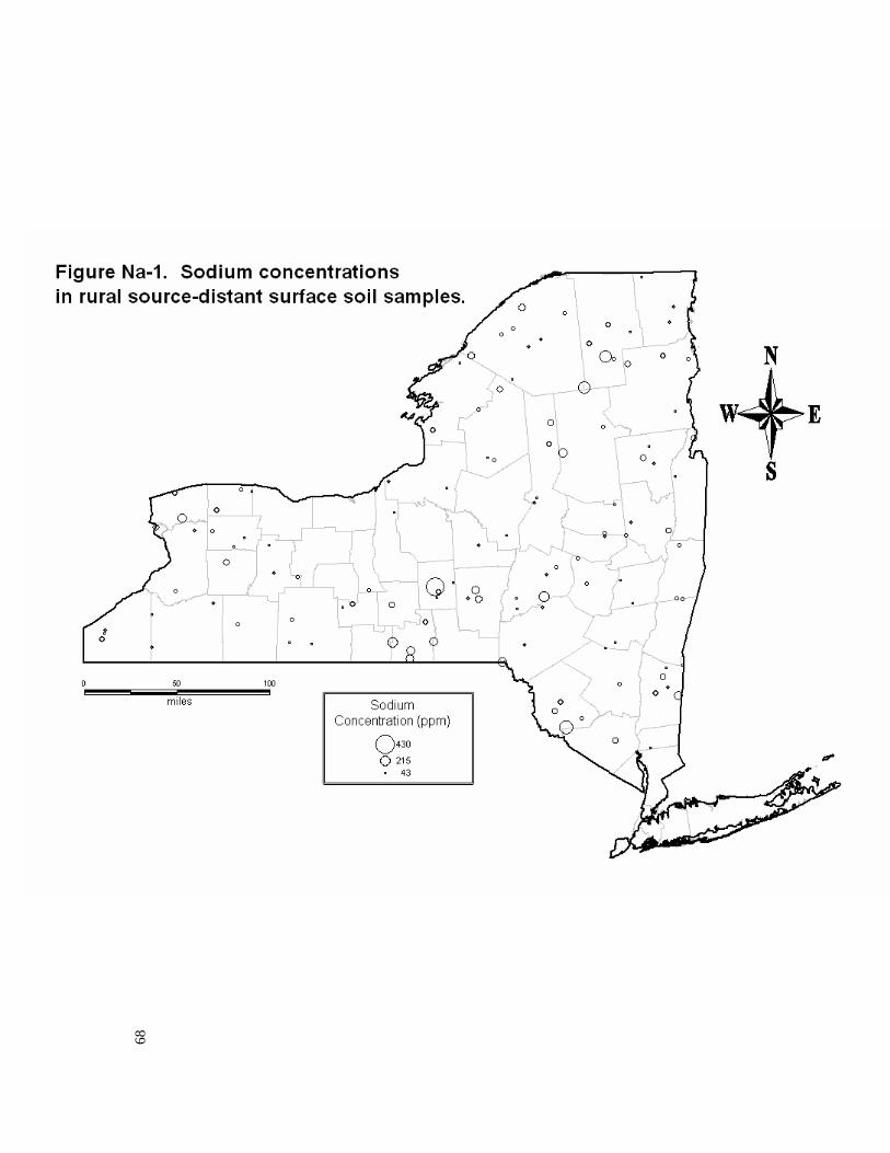
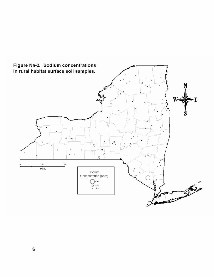
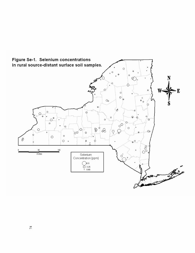
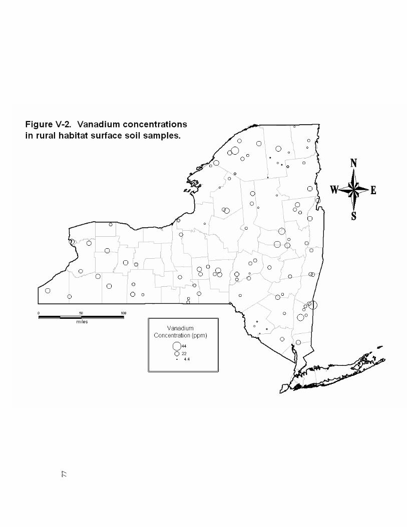
Figure Mg-1: Statewide Magnesium Concentration Map (Source-Distant) Figure Mg-2: Statewide Magnesium Concentration Map (Habitat) Figure Na-1: Statewide Sodium Concentration Map (Source-Distant) Figure Na-2: Statewide Sodium Concentration Map (Habitat) Figure Ni-1: Statewide Nickel Concentration Map (Source-Distant) Figure Ni-2: Statewide Nickel Concentration Map (Habitat) Figure Pb-1: Statewide Lead Concentration Map (Source-Distant) Figure Pb-2: Statewide Lead Concentration Map (Habitat) Figure Se-1: Statewide Selenium Concentration Map (Source-Distant) Figure Se-2: Statewide Selenium Concentration Map (Habitat) Figure V-1: Statewide Vanadium Concentration Map (Source-Distant) Figure V-2: Statewide Vanadium Concentration Map (Habitat) Figure Zn-1: Statewide Zinc Concentration Map (Source-Distant) Figure Zn-2: Statewide Zinc Concentration Map (Habitat)

LIST OF TABLES Table 1. Results of protocol conformance and missing data evaluations Table 2: Counties where soil samples were collected Table 3: Relative percent differences for field duplicate samples Table 4: Representation of rural New York State soil orders Table 5a. MDL ranges for analytes not detected in the source-distant data set Table 5b. MDL ranges for analytes not detected in the habitat area data set Table 5c. MDL ranges for analytes not detected in the near source data set Table 6a: Percentile values for source-distant data set Table 6b: Percentile values for habitat area data set Table 6c: Percentile values for near source data set

APPENDICES

Appendix A: Urban (non-rural) areas of New York State Appendix B: Example of the packet of materials provided to samplers Appendix C: Target analyte list Appendix D: Habitat Area Sampling Protocol, Quality Review, and Data Analysis

SUMMARY The statewide Survey to Describe Concentration Ranges for Selected Analytes in Rural New York State Surface Soils ("Rural Soil Survey") was conducted jointly by the New York State Departments of Environmental Conservation (NYS DEC) and Health (NYS DOH). The objective of the study was to define analyte concentration ranges in rural surface soils from points of human contact with soil and from habitat areas. Rural properties (n = 125) were randomly selected for sampling using a digitized grid map and a random number generator. Field staff collected at least two types of surface soil samples at each property: a "source-distant" sample and a "remote" sample. Source-distant samples were obtained from areas that were reasonable points of human contact with soil, such as yards and trails, but at least five meters distant from potential pollution sources such as trash, roads, driveways or structures. Remote samples were collected from areas that were at least 20 paces (about 15 meters) distant from margins of human activity. At a randomly selected subset of properties, staff also collected a "near source" soil sample near a roadway or driveway. After completion of sampling, NYS DEC staff reviewed field documentation and aerial photographs to identify a subset of remote samples that were collected from habitat areas marginally influenced by human activities. Soil samples were analyzed for selected volatile organic compounds, semi-volatile organic compounds, organochlorine pesticides, Aroclor mixtures of polychlorinated biphenyls, metals, amenable cyanide and total cyanide using analytical methods commonly employed during contaminated site investigations. Based on the review of laboratory analytical and quality control data it appeared that several organic compounds on the survey's analyte list that were reported in low concentrations (typically less than 100 parts-per-billion) in soil samples may not have actually been present in rural soils. Most of these organic compounds were solvents commonly employed in analytical laboratories, or plasticizers that may leach from plastics used during sampling (plastic trowels) or chemical analysis (e.g., caps, tubing). These compounds were not evaluated during the statistical analysis phase. The remaining data were accepted. Laboratory analytical data were received for 120 source-distant, 121 remote and 28 near source samples, for a total of 269 samples. The survey protocol called for the avoidance of orchards and characterization of analyte concentrations in habitat areas, so a reduced data set was created by excluding data from four samples collected at known orchards, as well as data from remote areas that were not habitat. The reduced data set contained laboratory analytical data for 118 source-distant, 96 habitat and 28 near source samples, for a total of 242 samples1. This report discusses analyses of the reduced data set unless otherwise indicated. The survey findings may be briefly summarized as follows: Volatile Organic Compounds (VOCs) Most survey VOCs were rarely if ever detected in rural soil samples. After removal of data points suspected of reflecting laboratory or field contamination, the most frequently detected VOC was m/p-xylene, which was detected in 8 of 242 samples (3.3%). The highest VOC concentration reported was 79 ppb for the solvent stabilizer 1,4-dioxane in a source-distant soil sample. Semi-volatile Organic Compounds (SVOCs) 1 Analytical results were not received for semi-volatile organic compounds in one habitat sample.

Most survey SVOCs were not detected in any rural soil samples, but several polycyclic aromatic hydrocarbons (PAHs) were detected, primarily in near source samples. Organochlorine Pesticides (OCPs) Survey OCP residues were detected in 2 of 242 rural soil samples (0.8%). Specifically, one source-distant soil sample contained 4,4-DDD, alpha-chlordane, gamma-chlordane and heptachlor epoxide at concentrations of 10 ppb or less, and another source-distant sample contained Endosulfan I at 15 ppb. No OCPs were detected in rural near source or habitat surface soils. Aroclor Mixtures of Polychlorinated Biphenyls (Aroclors) Survey Aroclors were detected in 4 of 242 rural soil samples (1.7%). Specifically, Aroclor 1016 was detected in one source-distant sample at a concentration of 72 ppb, and Aroclor 1260 was detected in one habitat sample and two near source samples at 47, 32 and 20 ppb, respectively. Elements (Metals) As expected, all survey metals except antimony, thallium and silver were detected in the majority of rural soil samples, and several metals were detected in all samples. Cyanide Neither total nor amenable cyanide was detected in any surface soil sample.

INTRODUCTION

In 2004, the New York State Departments of Environmental Conservation (NYS DEC) and Health (NYS DOH) developed a protocol for a statewide survey to characterize concentrations of selected analytes in rural surface soils. The protocol outlined a process for the random selection of rural properties for sampling and collection of soil samples in areas that were reasonable points of human contact, as well as soil samples from habitat areas. The public was notified of the survey in the May 19, 2004 Environmental Notice Bulletin, which provided a link to the draft survey protocol and established a 30-day comment period. The agencies also discussed the survey with stakeholders at public meetings held throughout the State in connection with the new Brownfield Cleanup Program. During the public comment period, the agencies received a number of verbal and written comments, many of which are addressed in this report. The draft survey protocol indicated that surface soil samples would be collected from points of human contact that were at least 20 paces from identifiable sources of soil contamination such as roads or structures. Some reviewers disagreed with this restriction, which excluded surface soils near common sources of diffuse pollution (e.g., roads, parking lots or driveways). While near-source analyte concentrations were not the focus of the survey, the survey was augmented to include sampling near rural roads and driveways. Reviewers of the original survey protocol also noted the potential for naturally elevated concentrations of some metals in some regions. The agencies agreed to provide elemental concentration maps to assist in assessing the potential for regional anomalies. Elemental concentration maps for all frequently detected metals (i.e., all except antimony and thallium) are provided in this report. Reviewers suggested that soil type should be an important consideration during survey design. Both soil type and land use may potentially influence concentrations of analytes. This was an important consideration during survey design and the probabilistic approach to selecting land parcels was intended to ensure representative sampling of rural soil types and rural land uses. Geographical information system (GIS) software was used to match sampling locations to soil orders and suborders, and reasonably representative sampling was confirmed. Feedback from field staff resulted in two changes to the survey protocol within the first days of soil sampling. The draft survey protocol indicated that source-distant surface soil samples would be collected from points of human contact that were at least 20 paces distant from roads, pavement, structures, outfalls, drainage swales or drip lines. Early in the implementation phase of the survey, the human contact and distance requirements for source-distant samples proved incompatible, and the minimum distance from sources was reduced to 10 meters or, if that was not possible, the greatest distance that could be obtained without leaving a property. Ultimately, a minimum distance of five meters from any potential pollution source was obtained for source-distant samples, with most samples collected at least 10 meters from any such source. The draft survey protocol also indicated that habitat surface soil samples would be collected at least 100 yards distant from the edge of areas of regular human activity such as yards, golf courses, farms, athletic fields, areas of fill, mines, roads, pavement, structures, burn barrels,

outfalls, drainage swales or drip lines, etc. The distance requirement for habitat samples proved difficult to obtain. In an effort to ensure a representative number of habitat soil samples, field staff collected soil from remote areas at least 20 paces (approximately 15 meters) from the edge of areas of regular human activity when possible, or otherwise from areas of limited human activity. These samples were termed "remote" samples. After implementation of the survey, NYS DEC staff reviewed sampling documentation and aerial photographs to identify a subset of 96 "habitat" samples -- remote samples that were collected from habitat areas marginally influenced by human activities.

A. PROJECT DESIGN

The survey was conducted jointly by the New York State Departments of Environmental Conservation (NYS DEC) and Health (NYS DOH). It consisted of four phases: (1) sample site selection, (2) sample collection and transport, (3) laboratory analysis and data reporting, and (4) data analysis. I. Purpose of the Statewide Survey The survey was conducted to determine concentration ranges for selected analytes in surface soils of rural New York State. The survey determined ranges for analytes in three types of surface soil samples:

• "Source-Distant" - surface soil samples from areas that were considered reasonable points of human contact, at least five meters from any potential pollution source

• "Remote" - surface soil samples from areas that were at least 20 paces (about 15 meters) distant from margins of regular human activity, unless that distance could not be obtained, in which case remote samples were collected from areas of limited human activity.

• "Near Source" - surface soil samples from areas typically two meters distant from a road or driveway.2

All samples were free of readily discernible contamination. After completion of sampling, NYS DEC staff reviewed field documentation and aerial photographs to identify a subset of 96 "habitat" samples -- remote samples that were collected from habitat areas marginally influenced by human activities. II. Definitions “Surface soil” was the uppermost five centimeters (for source-distant and near source samples) or 15 centimeters (for remote/habitat samples) of soil immediately below vegetative cover. In the absence of vegetative cover, surface soil was the uppermost five (or 15) centimeters of soil. “Rural” areas were those so designated by the United States census for the year 2000. The Census Bureau's classification of "rural" consisted of all territory, population, and housing units located outside of urbanized areas (UAs) and urban clusters (UCs). We delineated UA and UC boundaries to encompass densely settled territory, which consisted of:

• core census block groups or blocks that had a population density of at least 1,000 people per square mile, and

• surrounding census blocks that had an overall density of at least 500 people per square

mile.

2 In some cases, near source samples were collected more than two meters (up to about three meters) from a road or driveway.

UAs consisted of contiguous, densely settled census blocks that met minimum population density requirements, along with adjacent densely settled census blocks that together encompassed a population of at least 50,000 people. UCs consisted of contiguous, densely settled census block groups and census blocks that met minimum population density requirements, along with adjacent densely settled census blocks that together encompassed a population of at least 2,500 people, but fewer than 50,000 people.3 Under certain conditions, less densely settled territory was considered to be part of each UA or UC. UAs and UCs for New York State are listed in Appendix “A.” “Reasonable point of human contact” referred to a place where people have a regular opportunity to contact soil. This included such places as residential yards, farms, and parks (near trails), but excluded such places as swamps, bogs, and paved areas. “Readily Discernable Contamination” was that which was known or suspected based on current or past site uses, proximity to major pollution sources, or conditions encountered during soil sampling such as the presence of waste, unusual odors, or unusual discoloration. "Habitat areas marginally influenced by human activities" or “habitat areas” were locations that (1) provided environmental conditions that could sustain plant and animal life and (2) were at least 15 meters distant from the edge of areas of regular human activity such as yards, golf courses, farms, athletic fields, areas of fill, mines, etc. III. Number of Samples Collected In selecting source-distant and remote locations to sample, consideration was given to the number required to establish the nature of concentration distributions for individual contaminants, accounting for potential loss of data due to quality control and logistical considerations. The number of near source sampling locations was selected based on the number needed to evaluate differences between concentrations of analytes in near source and paired source-distant samples. A more detailed discussion of sample number determination and statistical power considerations follows. Source-Distant and Remote Samples. When determining the number of source-distant and remote samples, the agencies considered statistical power and sampling density (samples collected per square-kilometer). StudySize version 1.0.8 (CreoStat HB, Sweden) was used to generate statistical power curves. Concentration distributions were expected to vary among the many survey analytes and the specifics of those distributions (e.g., means, standard deviations) were uncertain. The agencies therefore took a generic approach when examining the relationship between sample number (n) and statistical power. Specifically, the influence of sample n on the width of a 95 percent confidence interval around the mean concentration of an anlayte was assessed.4 The results indicated that the width of a confidence interval around the mean shrinks substantially up to about 100 samples, after which the shrinkage is less pronounced as more samples are added.

3 http://www.census.gov/geo/www/ua/uafedreg031502.pdf accessed in March 2004. 4 A standard deviation (SD) of 0.3 was assumed, with no mean specified. Although the widths of confidence intervals will depend on the assumed SD, shapes of the power curves are independent of the mean or assumed SD.

This suggests that a survey target of about 125 samples would strike an efficient balance between statistical power and cost considerations. The sampling density that would be achieved by the proposed survey target of 125 samples was compared to the sampling density achieved by Shacklette and Boerngen5 in their nationwide survey, which remains a commonly cited source of data on background concentrations of metals in soil.6 For most metals of interest, Shacklette and Boerngen collected and analyzed 25 soil samples from (mostly) rural fields in New York State. That number of samples corresponds to about one sample per 4,400 square kilometers of rural land. The proposed survey target of 125 samples would achieve a sampling density of about one sample per 900 square kilometers of rural land. Based on statistical power and sampling density considerations, the agencies set a target of 125 source-distant and 125 remote surface soil samples. Near Source Samples. Power calculations assumed that near source samples would be matched with source-distant samples, and that Student's paired t-test would be used to compare analyte concentrations in near source and source-distant samples. Once again, the agencies took a generic approach when examining the relationship between sample number (n) and statistical power. Specifically, the impact of increasing n on the magnitude of the mean difference in analyte concentrations that would be statistically significant was assessed. 7 The magnitude of the difference shrinks substantially up to about 25 or 30 samples, after which the shrinkage is less pronounced with added samples. This suggested that a survey target of about 30 near source samples would strike an efficient balance between statistical power and cost considerations. The agencies recognized that violations of t-test distribution assumptions would occur for some survey analytes, possibly leading to the use of distribution-free statistical tests. In general, such tests were expected to be somewhat less powerful than Student's paired t-test for differences following a normal distribution, but more appropriate -- and potentially more powerful -- for differences not following a normal distribution. Based on statistical power considerations, the agencies set a target of 31 near source soil samples. IV. Sample Site Selection Determination of Sampling Areas. Geographic information system (GIS) software (MapInfo Professional Version 7.0, MapInfo Corporation, Troy, NY) was used to create a map of New York State indicating areas designated as “rural” by the United States Census Bureau. A grid comprised of one-kilometer square cells, created several years ago for an unrelated GIS project, was laid over the State map such that approximately 125,000 cell centroids fell within the State boundaries, excluding off-shore waters. Each centroid was consecutively numbered 5 Shacklette, H.T., and Boerngen, J.G., 1984, Element concentrations in soils and other surficial materials of the conterminous United States: U.S. Geological Survey Professional Paper 1270, 105 p. 6 Shacklette and Boerngen did not survey surface soil, but rather subsurface soil collected from about 20 centimeters beneath the ground surface. Although some regional soils have been characterized for some analytes, we do not know of any other representative statewide data on contaminant concentrations in surface soil. 7 80 percent power and an alpha of 0.05 were assumed.

beginning in the upper left-hand corner and proceeding from left to right along the first row, and similarly along ensuing rows from top to bottom, until all centroids possessed a unique number. Randomly selecting 125 sampling areas from among approximately 125,000 cell centroids across the State could have resulted in large land areas (i.e., land areas of more than 50 miles in radius) without sampling sites. In order to decrease the likelihood of creating large gaps during assignment of sampling areas, the State map was divided into five nearly equal regions containing approximately 25,000 cell centroids each. Five regions were chosen because that number allowed for the dispersion of points across the State without excluding any large land areas. The first three regions began at the westernmost, northernmost and southernmost points in New York State and extended east, south and north (respectively) until approximately 25,000 cell centroids were encompassed. The fourth and fifth regions were created by dividing the remaining land area in half. For each of the five regions, cell centroids were ordered by their unique identifiers from the lowest to the highest, and then renumbered from one to about 25,000, with the maximum depending on the exact size of the region. For each region, a random number generator was employed to create a list of unique whole numbers ranging from one to the number of centroids in the region. Beginning at the top of the random number list, the first centroid located on accessible rural land was designated as the first sampling area, the second centroid located on accessible rural land was designated the second sampling area, and so on until 25 sampling areas were designated. The total number of designated areas across the State was 25 areas x 5 regions = 125 areas. For each region, a list of five alternative areas was generated using the next five numbers on the region's random number list. When designated sampling areas proved inappropriate, areas from the list of alternatives were selected to achieve the target of 125 soil samples, as summarized below. Rejected Sampling Areas. There were 25 original sampling areas randomly designated in each of the five regions, along with five randomly designated alternative sites. Four initially designated sampling areas not meeting the survey requirements (two each in the Northern and Western Regions) were replaced by alternatives as follows: Northern Region

An initial, randomly selected sampling area was located in a water body in Franklin County. This sampling area was replaced with a randomly selected alternative area in St. Lawrence County. An initial, randomly selected sampling area was located in a sparsely inhabited region of St. Lawrence County, on land owned by a bankrupt paper manufacturer (Deferiet Paper Company). The paper manufacturer was the sole landowner within a mile of the sampling area and the firm's successor in interest could not be determined. This sampling area was replaced with a randomly selected alternative area in Franklin County.

Western Region

An initial, randomly selected sampling area was located near two inactive hazardous waste disposal sites in Orleans County. This sampling area was replaced with a randomly selected alternative area in Steuben County.

An initial, randomly selected sampling area was located at an inactive hazardous waste disposal site in Cattaraugus County. This sampling area was replaced with a randomly selected alternative area in Cattaraugus County.

After the changes indicated above, a total of 125 sampling areas were designated for collection of matched source-distant and remote surface soil samples. A near source sample was designated at approximately every fourth sampling area, creating a subset of 31 areas where near source samples were to be collected. Permission to Sample. Names, addresses, and telephone numbers of property owners were obtained using the State’s database of real property records and community telephone directories. Verbal permission to collect soil samples was obtained from property owners by telephone prior to entering the field. When permission to sample could not be obtained from the owner of an originally designated property, the nearest property where permission to sample could be obtained was selected for sampling, provided that it was no more than one mile from the initial sampling point. Some property owners either did not respond to telephone calls or elected not to participate. As a result, staff telephoned 284 property owners before gaining permission to sample at 125 properties. Determination of Sampling Points. Geographic coordinates and maps indicating designated sampling areas were provided to field staff, who proceeded to the areas and evaluated sampling opportunities. If a designated sampling area could not be accessed by automobile, field staff proceeded as near as possible to the designated area. To characterize a reasonable point of human exposure, staff then sampled the nearest point that was:

• Primarily soil (rather than rock, gravel, peat, etc.) • Free of unusual odors, discoloration or non-soil materials (like trash) • If possible, at least 20 paces (about 15 meters) distant from roads, pavement,

structures, outfalls, drainage swales or drip lines8 • At least one-half mile from an active or inactive industrial facility, waste disposal site,

orchard9, or other major pollution source • Not in a swamp, bog, wilderness or other area where soil contact is rare • Otherwise a reasonable point of potential human exposure

8 The original survey goal of collecting source-distant samples from points of human contact that were at least 20 paces from any sources of contamination was modified to reflect conditions reported by field staff. Staff sometimes could not locate a reasonable point of human contact at a distance of 20 paces from any source, so the required distance was reduced. 9 Soil at active and former orchards is sometimes contaminated with agricultural chemicals, such as lead arsenate.

A near source sample was also collected at designated locations. The exact sampling location was along an imaginary line extending from the site of the source-distant sample to the nearest roadway or driveway, and approximately two meters from the roadway or driveway. Remote samples were collected at all properties according to instructions provided by NYS DEC staff. Remote areas were:

• Primarily soil (rather than rock, gravel, peat, etc.)

• Free of unusual odors, discoloration or non-soil materials

• If possible, at least 20 paces (about 15 meters) distant from the edge of areas of regular human activity such as yards, golf courses, farms, athletic fields, areas of fill, mines, roads, pavement, structures, burn barrels, outfalls, drainage swales or drip lines, etc.10

• At least one-half mile from an active or inactive industrial facility, waste disposal

site, orchard, or other major pollution source

• In areas not inundated by water at the time of the sample collection V. Sample Collection and Transport Sampling instructions were included in the packet of materials provided to samplers (see Appendix "B"). Samples were collected using clean plastic or stainless steel trowels to fill glass bottles with soil. Stainless steel trowels were only used on rare occasions when the ground was too hard for plastic trowels. Rocks and large soil fragments were excluded. Soil samples were collected from the uppermost five centimeters (for source-distant and near source samples) or 15 centimeters (for remote samples) of soil immediately below vegetative cover. In the absence of vegetative cover, surface soil was the uppermost five (or 15) centimeters of soil. In most cases, the location of each sample was logged in a manner that provided enough information to geocode the sampling point in a geographic information system. In some cases, this information was not available and the sampler designated the sampling location using aerial photographs overlain onto a GIS map. Sometimes sampling locations were determined from samplers’ field notes, which included descriptions of the immediate area including roads, trails, structures, litter, waterways and prominent land features if present. In many cases the sampling area was also photo-documented and descriptions of each photograph were recorded. Transportation and Chain of Custody. At each location, separate soil samples were collected for each laboratory analysis as per laboratory requirements and duplicate samples (source-

10 The original survey goal of collecting samples from habitat areas at least 100 yards from the margin of human activity was modified to reflect conditions reported by field staff. Staff sometimes could not obtain a sample at a distance of 100 yards, so the minimum distance was reduced.

distant and remote/habitat) were collected for archiving. After collection, samples for laboratory analysis were chilled and mailed to a designated DEC contract laboratory for analysis. Archive samples were sent to the Wadsworth Center in Albany, New York, where they are being held pending further analyses.11 Field staff followed normal chain of custody procedures and a chain of custody form accompanied samples. Sampling Personnel. Field work was performed by agency staff familiar with environmental sampling. VI. Laboratory Analysis and Data Reporting Chemtech Environmental, Inc. of Mountainside, New Jersey, a NYS DEC contract laboratory accredited for all relevant analyses by the NYS DOH Environmental Laboratory Approval Program (ELAP), analyzed the soil samples. Chemtech provided NYS DEC Analytical Services Protocol (ASP) deliverables including data validation packages that were further reviewed by NYS DEC staff with expertise in the field of analytical chemistry. Survey analytes were those found on target compound and target analyte lists for laboratory analytical methods routinely applied at contaminated sites, as follows:

• Volatile Target Compound List [US EPA Method 8260B] • Semivolatile Target Compound List [US EPA Method 8270C] • Pesticides/Aroclors (PCBs) - Target Compound List [US EPA Methods 8081A

and 8082]

• Target Analyte List metals [US EPA Method 6010B (metals except Hg) and US EPA Method 7471A (Hg)]

• Total and amenable cyanide [US EPA Method 9012A]

Each list is attached to this document (see Appendix “C”). All concentration data were reported on an analyte weight per dry soil weight basis. Organic analyte concentrations were reported in micrograms per kilogram (parts-per-billion or "ppb"). Inorganic analyte concentrations were reported in micrograms per gram (parts-per-million or "ppm"). Detection and reporting limits were those specified by the methods and were consistent with limits achieved during investigations of contaminated sites. Quality Assurance/Quality Control. Some surface soil samples were analyzed in duplicate or spiked to assess precision and bias. Surrogates were employed as required to confirm adequate recovery. Organic and inorganic analyses included one field duplicate sample analysis for approximately every 10 samples collected. Laboratory analytical results from field duplicate samples were only used for comparisons with results from primary samples. The purpose of these comparisons was to quantify the combined geospatial/laboratory analytical variability encountered. 11 No determinations have been made regarding laboratory analyses of archived soil samples.

Chemtech performed initial reviews of laboratory data quality before data reports were issued to the NYS DEC. NYS DEC staff then performed an independent data validation review. VII. Assignment of Soil Order and Suborder Concentrations of analytes in soils may be influenced by anthropogenic and natural factors. One of the more important natural factors is soil type. For example, clay minerals sometimes concentrate trace elements (Jiang et al., 2005), and background concentrations of elements in surface soils can vary greatly based on soil order and suborder (Chen et al., 2002). The rural survey sampling locations were evaluated to confirm that a representative subset of rural soil types were sampled. Soil types may be defined in a number of ways. The rural soil survey employed the soil scheme used by the United States Department of Agriculture. Soil order is the highest category in the USDA soil taxonomy, distinguishing soils in relation to the five soil-forming factors (climate, organisms, parent material, time and relief). A map of USDA soil orders and soil suborders was created using MapInfo Professional Version 7.0 (MapInfo Corporation, Troy, NY), employing data from the State Soil Geographic (STATSGO) database for New York State. This map was used to generate a summary table allowing the agencies to confirm representative sampling of soil orders.

B. DATA ANALYSIS METHODS

I. ASSESSMENT OF DATA QUALITY Laboratory analytical packages were reviewed by the contract laboratory and NYS DEC Division of Remediation staff to identify data quality concerns. Data qualifiers were evaluated and results from dilution re-analyses of samples were substituted for initial results that were outside of the instrument calibration range. Blank contamination was noted and assessed for data quality implications. The contract laboratory assigned a number of qualifiers based on its reviews, including “J” qualifiers indicating estimated concentrations and, very rarely, “E” qualifiers indicating concentrations outside the calibration range. Estimated concentrations were accepted as detected values for purposes of constructing data bases. When "E" qualifiers were encountered, the results of follow-up analyses were substituted for the original qualified values. Field sampling notes, photo-documentation and aerial photographs were reviewed and samplers were interviewed to confirm conformance with the survey protocol. Differences in analyte concentrations between primary and field duplicate samples were evaluated using SAS (SAS Institute Inc., Cary, N.C.). Relative percentage differences (RPD) between analyte concentrations in sample pairs were computed as RPD = [2(x1 – x2)/(x1 + x2)]100%. Mean RPDs for anlaytes were also calculated. Only analytes detected in at least 10 percent of rural soil samples were considered during RPD assessments. II. DISTRIBUTION OF SAMPLING LOCATIONS Sampling locations were plotted using a GIS (MapInfo) to generate maps illustrating the survey’s spatial coverage. GIS was employed to generate a table indicating the number of samples collected in each county. III. DESCRIPTIVE STATISTICS A. Analytes Not Detected. For each data set (source-distant, habitat and near source), analytes not detected in any sample were listed and their method detection limits were summarized using minima and maxima. These analytes were not considered further. B. Detected Analytes. For each data set (source-distant, habitat and near source), concentration distributions for all analytes detected in at least one sample were summarized using percentiles calculated employing the empirical distribution function with averaging, which is the SAS default for determining percentile values. Data filling techniques were sometimes required to address “non-detects” (i.e., analyte concentrations below MDLs). Such data were converted to the MDL prior to calculating percentiles, and "less than" signs were inserted into percentile tables to indicate when analytes were not detected. Percentiles that are MDL values merely reflect the distribution of MDLs and do not necessarily reflect distributions of analyte concentrations.

The geospatial distributions of metals that were detected in the majority of rural soil samples were illustrated by plotting sampling points on maps. The size of each point corresponded to the magnitude of the concentration value reported.

C. RESULTS

I. ASSESSMENT OF DATA QUALITY Analytes Not Considered. The laboratory analytical data were validated by the contract laboratory and were further reviewed by NYS DEC staff with expertise in the field of analytical chemistry. Based on issues identified during the review of laboratory analytical and quality control data, as well as staff experience at contaminated sites, the following organic chemicals were present, or may have been present, in one or more rural surface soil samples solely or in part due to laboratory or field contamination of soil samples: acetone, chloroform, 2-butanone, dibutyl-n-phthalate, ethanol, methylene chloride, phenol, 1,2,4-trichlorobenzene, cyclohexane, bis(2-ethylhexyl)phthalate, butylbenzylphthalate, tetrachloroethylene and trichlorofluoromethane. Most of these are solvents commonly employed in analytical laboratories and plasticizers that may leach from plastics used during sampling (plastic trowels) or chemical analysis (caps, tubing). These chemicals were not evaluated during the statistical analysis phase. In addition, two toluene observations were removed due to apparent laboratory contamination. The remaining data were deemed suitable for the intended purposes of the survey. Missing Values. One near source sample was not collected. In addition, analytical results were not received for five source-distant, four habitat, and two near source samples that were collected (see Table 1). These factors reduced sample numbers to 120 source-distant, 28 near source, and 121 habitat samples. Analytical results were not received for semi-volatile organic compounds in one habitat sample. Delta-BHC results were only reported for 39 source-distant, 10 near source and 62 habitat samples. Protocol Adherence. A review of aerial photographs of sampling areas, sampling photo-documentation, and samplers' field notes indicated divergence from the survey protocol at some sampled land parcels (see Table 1). Owners of two rural properties reported that the properties were formerly orchards. Laboratory analytical data for samples collected on these properties were not used because the survey protocol prohibited sampling at known orchards. Although the original survey protocol called for remote/habitat samples to be collected at least 100 yards distant from the margin of human activity, practical constraints during sampling resulted in a reduction of the minimum distance to 20 paces (about 15 meters). Remote/habitat samples were collected at all properties, but later reviews of collection photographs, field notes and aerial photography indicated that 25 properties did not include habitat areas conforming to even the modified survey protocol (see Table 1 and Appendix D). The 25 remote samples collected laboratory analytical data for 25 remote samples that did not conform to the modified protocol were not considered during the data analysis. Several properties were not large or diverse enough to allow for the originally required distance of 20 paces (about 15 meters) between the source-distant soil sample and the nearest road or driveway. Field staff advised survey staff of the problem within one day of commencing sampling efforts. The absence of acceptable sampling locations suggested a need for greater flexibility in the definition of suitable soils. The protocol was therefore modified and survey staff were allowed to collect source-distant samples as near as five meters from a potential source. However, the original requirement of 20 paces was achieved at the majority of properties.

One rural property was sampled despite the presence of an inactive hazardous waste disposal site about one-quarter mile away. Laboratory analytical data for the soil samples collected on that property were retained for purposes of background determinations because site investigations established a low potential for off-site migration of site contaminants. A review of analyte concentrations in the sample supported this judgement, identifying no unusual patterns. In summary, removal of data for samples collected at locations inconsistent with the survey protocol reduced the number of source-distant samples collected to 118. A similar analysis performed on the habitat sampling locations reduced that data set to 96 samples. Field Duplicate Samples. Field quality control information, which consisted of field duplicate samples, was reviewed. There were 24 pairs of field duplicate samples collected and analyzed in the study. These included 11 source-distant pairs, 3 near source pairs and 10 habitat pairs. The 24 pairs of field duplicate samples represent an approximate 1:10 frequency of soil sample duplication for the planned survey. Field duplicate samples were analyzed for all survey target analytes, resulting in a total of 4,218 possible RPD comparisons, but many of these comparisons were for analytes that were never or rarely detected in paired samples. Analysis of field duplicates included the calculation of relative percent differences (RPDs) and these results are provided in Table 3 for selected PAHs and metals (those that had over 60 percent detected values in any data set). We established a screening criterion of +/- 50 percent RPD for each observation in field duplicate analyses; the reported field duplicate data are evaluated against this criterion.12 RPDs were not calculated for pairs in which one or both of the results were below the limit of detection. For the selected PAHs and metals, a total of 18 of the 471 calculated RPDs (4 percent) exceeded the +/- 50 percent criterion: 1 of 24 for aluminum, 2 of 20 for arsenic, 1 of 24 for barium, 2 of 20 for cadmium, 1 of 24 for chromium, 1 of 24 for iron, 2 of 24 for magnesium, 1 of 24 for manganese, 2 of 24 for mercury, 2 of 24 for nickel, 1 of 24 for selenium, and 2 of 16 for sodium. The largest RPDs were of 100, 93, 90 and 86 percent for selenium, arsenic, cadmium and nickel, respectively. Based on analytical results for laboratory duplicate analyses, which indicated acceptable precision, some of the larger RPDs appear to have resulted from intrinsic variability in analyte concentrations at some sampling locations. Representation of Rural Soil Orders. Figure 1 illustrates the geospatial distribution of soil orders in New York State. Of the 12 soil orders, seven are recognized in New York State. These are Alfisols, Entisols, Histosols, Inceptisols, Mollisols, Spodosols and Utilisols. Three soil orders predominate in rural settings: Alfisols, Inceptisols and Spodosols. As the agencies selected sampling locations at random, the three dominant soil orders of rural New York State were sampled approximately in proportion to their prevalence in rural settings (see Table 4). Elemental concentrations may differ among soil suborders as well, but probabilistic sampling resulted in proportional representation of rural soil suborders. 12 This is more than the conventional criterion of 20 percent used for duplicate samples collected as "split samples" from a well-mixed composite sample. The higher criterion was established to account for increased variability in analyte concentrations due to collection of two discrete (not split) samples.

II. DISTRIBUTION OF SAMPLING LOCATIONS The final sampling locations are indicated in Figure 2 (for source-distant samples) Figure 3 (for habitat samples) and Figure 4 (for near source samples). The counties where samples were collected are indicated in Table 2. III. DESCRIPTIVE STATISTICS Tables 5a,b and c indicate analytes that were not detected in rural soil samples, along with corresponding MDL ranges. Analyte concentration percentiles (quantiles) for each sample type (source-distant, near source and habitat are reported in Tables 6a, b and c. Percentile values preceded with "<" ("less than") are MDLs and do not indicate actual analyte detections. On rare occasions, one or more MDL values for an analyte exceeded an actual detection. In such cases the detected level occupied a lower percentile rank than the MDL and the analyte's maximum value was flagged with an asterisk.

References: Chen M, Ma LQ & Harris W.G. (2002) Arsenic concentrations in Florida surface soils: influence of soil type and properties. Soil Sci. Soc. Am. J. 66:632-640. Jiang W, Zhang S, Shan X et al. (2005) Adsorption of arsenate on soils. Part 2: Modeling the relationship between adsorption capacity and soil physiochemical properties using 16 Chinese soils. Environ. Pollution 138:285-289.

APPENDIX “A”

URBANIZED AREAS AND URBAN CLUSTERS

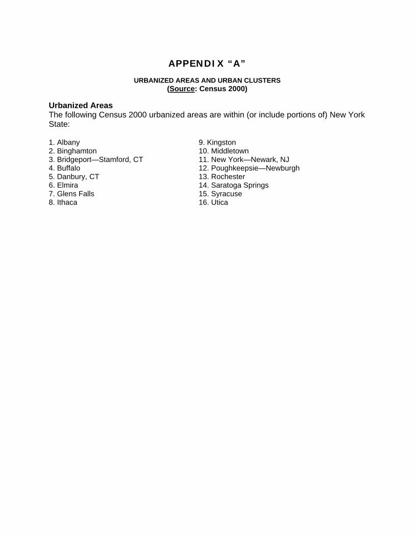
(Source: Census 2000) Urbanized Areas The following Census 2000 urbanized areas are within (or include portions of) New York State: 1. Albany 2. Binghamton 3. Bridgeport—Stamford, CT 4. Buffalo 5. Danbury, CT 6. Elmira 7. Glens Falls 8. Ithaca

9. Kingston 10. Middletown 11. New York—Newark, NJ 12. Poughkeepsie—Newburgh 13. Rochester 14. Saratoga Springs 15. Syracuse 16. Utica

Urban Clusters The following Census 2000 urban clusters are within (or include portions of) New York State:

1. Akron 41. Hamilton 81. Plattsburgh2. Albion 42. Hamlin (town) 82. Port Jervis3. Alfred 43. Highland Mills 83. Potsdam4. Amsterdam 44. Holley 84. Ravena5. Arcade 45. Hoosick Falls 85. Red Hook6. Attica 46. Hornell 86. Rhinebeck7. Auburn 47. Hudson 87. Riverhead8. Avon 48. Ilion—Herkimer 88. Rome9. Batavia 49. Jamestown 89. Sag Harbor10. Bath 50. Lake Placid 90. Salamanca11. Bradford, PA 51. Le Roy 91. Saranac Lake12. Brocton 52. Liberty 92. Sayre, PA--Waverly, NY13. Caledonia 53. Lima 93. Scottsville14. Canajoharie 54. Little Falls 94. Sidney15. Canandaigua 55. Livonia 95. Silver Creek16. Canton 56. Lockport 96. Skaneateles17. Carthage 57. Lowville 97. Sodus18. Catskill 58. Lyons 98. Southold19. Cazenovia 59. Malone 99. Springs20. Chittenango 60. Massena 100. Springville21. Churchville 61. Mattituck 101. Ticonderoga (town)22. Cobleskill 62. Mechanicville 102. Tupper Lake23. Cold Spring 63. Medina 103. Valatie24. Corinth 64. Montgomery—Maybrook 104. Walton25. Corning 65. Monticello 105. Walworth (town)26. Cortland 66. Moravia 106. Warrensburg27. Coxsackie 67. Mount Morris 107. Warsaw28. Dannemora 68. Newark 108. Warwick29. Dansville 69. Newfane 109. Watertown30. Dryden 70. New Paltz 110. Watkins Glen31. Dunkirk—Fredonia 71. Norwich 111. Weedsport32. Ellenville 72. Ogdensburg 112. Wellsville33. Geneseo 73. Olean 113. Westfield34. Geneva 74. Oneida 114. West Hurley35. Gloversville 75. Oneonta 115. Woodridge36. Goshen 76. Oswego 116. Wurtsboro37. Gouverneur 77. Owego38. Gowanda 78. Pawling39. Granville 79. Penn Yan40. Greenwich 80. Perry

APPENDIX “B”

RURAL BACKGROUND SOIL SURVEY DETAILED SOIL SAMPLE COLLECTION PROTOCOL

1. Envision a square of sufficient size to fill the jars required. We guess that this may be from 10 x 10 to 25 x 25 inches wide, depending on sampling depth and how many bottles you need to fill. 2. Clear away vegetative cover, if any, from the square. If collecting only a regular sample with no duplicate, fill:

a. One 8-oz. jar and one 2-oz. jar using soil from various portions of the square b. One 8-oz. (archive) jar using soil from various portions of the square

If collecting both a regular sample and a duplicate, divide the square into four roughly equal quadrants ...

1 2

3 4

... and fill:

a. One 8-oz. jar and one 2-oz. jar using only soil from quadrants 1 and 4 (this is the regular sample) b. One 8-oz. jar and one 2-oz. jar using only soil from quadrants 2 and 3 (this is the dupe) c. One 8-oz. jar using soil from all four quadrants (this is the archival sample)

NOTES For regular health samples ("source-distant" and "near source"), their archivals, and their duplicates, please scrape to a depth of 2 inches b.g.s. For habitat samples, their archivals, and their duplicates, please scrape or dig to a depth of 6 inches b.g.s. Please exclude pebbles, stones and roots to the extent possible.

APPENDIX “C”

Rural Soil Survey Analytes

Rural Soil Survey Target Compound List for Volatiles by USEPA 8260B

COMPOUND CAS # COMPOUND CAS #

Dichlorodifluoromethane 75-71-8 trans-1,2-Dichloropropene 10061-02-6Chloromethane 74-87-3 1,1,2-Trichloroethane 79-00-5Bromomethane 74-83-9 Tetrachloroethene 127-18-4Vinyl chloride 75-01-4 2-Hexanone 591-78-6Chloroethane 75-00-3 Dibromochloromethane 124-48-1Trichlorofluormethane 75-69-4 1,2-Dibromoethane 106-93-41,1-Dichloroethene 75-35-4 Chlorobenzene 108-90-71,1,2-Trichloro-1,2,2-trifluoroethane 76-13-1 Ethylbenzene 100-41-4Acetone 67-64-1 m-Xylene 108-38-3Carbon disulfide 75-15-0 o-Xylene 95-47-6Methyl acetate 79-20-9 p-Xylene 106-42-3Methylene chloride 75-09-2 Naphthalene 91-20-3trans-1,2-Dichloroethene 156-60-5 Styrene 100-42-5Methyl-tert-butyl ether 1634-04-4 Bromoform 75-25-21,1-Dichloroethane 75-34-3 Isopropylbenzene 98-82-8cis-1,2-Dichloroethene 156-59-2 1,1,2,2-Tetrachloroethane 79-34-52-Butanone 78-93-3 1,3-Dichlorobenzene 541-73-1Chloroform 67-66-3 1,4-Dichlorobenzene 106-46-71,1,1-Trichloroethane 71-55-6 1,2-Dichlorobenzene 95-50-1Cyclohexane 110-82-7 1,2-Dibromo-3-chloropropane 96-12-8Carbon tetrachloride 56-23-5 1,2,4-Trichlorobenzene 120-82-1Benzene 71-43-2 Ethanol 64-17-51,2-Dichloroethane 107-06-2 Methanol 67-56-1Trichloroethene 79-01-6 tert-Butanol 75-65-0Methylcyclohexane 108-87-2 p-Isopropyltoluene 99-87-61,2-Dichloropropane 78-87-5 1,2,4-Trimethylbenzene 95-63-6Bromochloromethane 75-27-4 1,3,5-Trimethylbenzene 108-67-8cis-1,3-Dichloropropene 10061-01-5 sec-Butylbenzene 135-98-84-Methyl-2-pentanone 108-10-1 tert-Butylbenzene 98-06-6Toluene 108-88-3 n-Butylbenzene 104-51-8

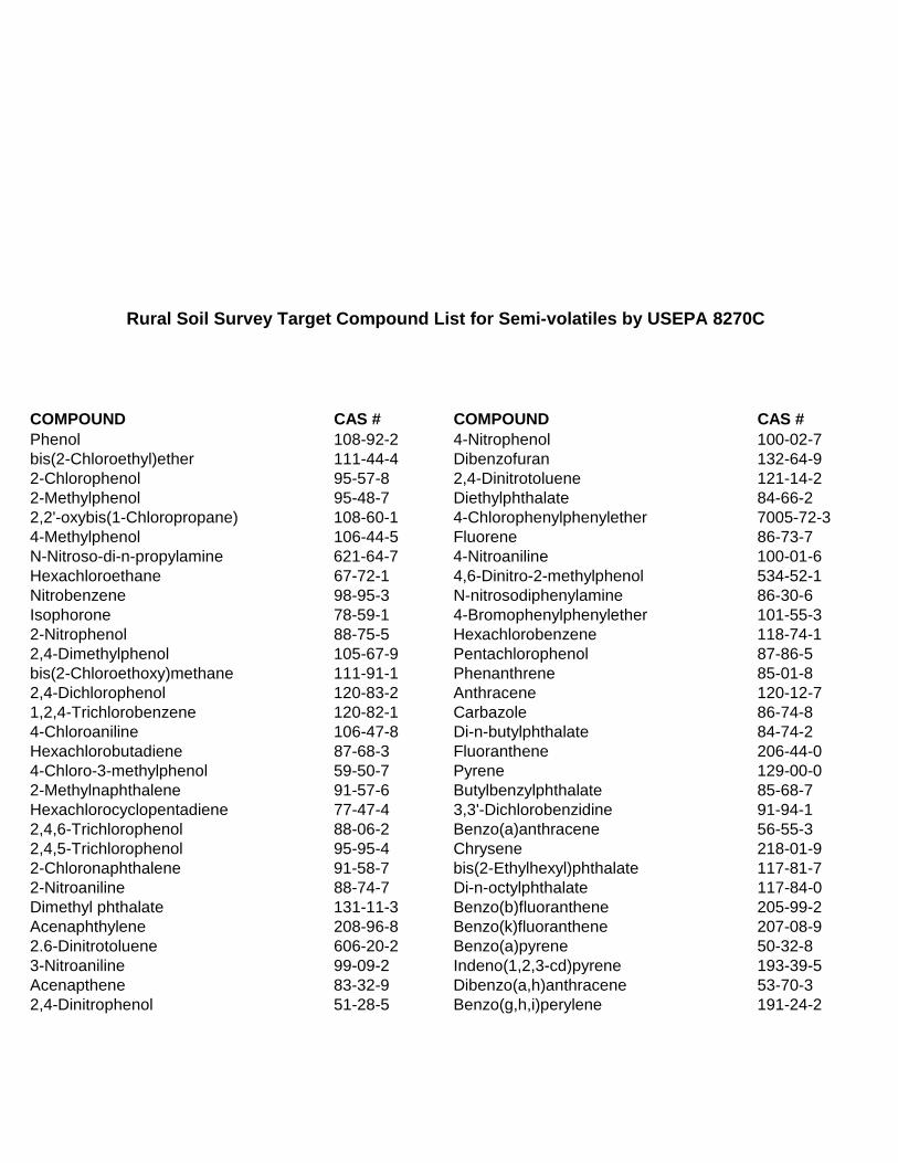
Rural Soil Survey Target Compound List for Semi-volatiles by USEPA 8270C COMPOUND CAS # COMPOUND CAS #

Phenol 108-92-2 4-Nitrophenol 100-02-7bis(2-Chloroethyl)ether 111-44-4 Dibenzofuran 132-64-92-Chlorophenol 95-57-8 2,4-Dinitrotoluene 121-14-22-Methylphenol 95-48-7 Diethylphthalate 84-66-22,2'-oxybis(1-Chloropropane) 108-60-1 4-Chlorophenylphenylether 7005-72-34-Methylphenol 106-44-5 Fluorene 86-73-7N-Nitroso-di-n-propylamine 621-64-7 4-Nitroaniline 100-01-6Hexachloroethane 67-72-1 4,6-Dinitro-2-methylphenol 534-52-1Nitrobenzene 98-95-3 N-nitrosodiphenylamine 86-30-6Isophorone 78-59-1 4-Bromophenylphenylether 101-55-32-Nitrophenol 88-75-5 Hexachlorobenzene 118-74-12,4-Dimethylphenol 105-67-9 Pentachlorophenol 87-86-5bis(2-Chloroethoxy)methane 111-91-1 Phenanthrene 85-01-82,4-Dichlorophenol 120-83-2 Anthracene 120-12-71,2,4-Trichlorobenzene 120-82-1 Carbazole 86-74-84-Chloroaniline 106-47-8 Di-n-butylphthalate 84-74-2Hexachlorobutadiene 87-68-3 Fluoranthene 206-44-04-Chloro-3-methylphenol 59-50-7 Pyrene 129-00-02-Methylnaphthalene 91-57-6 Butylbenzylphthalate 85-68-7Hexachlorocyclopentadiene 77-47-4 3,3'-Dichlorobenzidine 91-94-12,4,6-Trichlorophenol 88-06-2 Benzo(a)anthracene 56-55-32,4,5-Trichlorophenol 95-95-4 Chrysene 218-01-92-Chloronaphthalene 91-58-7 bis(2-Ethylhexyl)phthalate 117-81-72-Nitroaniline 88-74-7 Di-n-octylphthalate 117-84-0Dimethyl phthalate 131-11-3 Benzo(b)fluoranthene 205-99-2Acenaphthylene 208-96-8 Benzo(k)fluoranthene 207-08-92.6-Dinitrotoluene 606-20-2 Benzo(a)pyrene 50-32-83-Nitroaniline 99-09-2 Indeno(1,2,3-cd)pyrene 193-39-5Acenapthene 83-32-9 Dibenzo(a,h)anthracene 53-70-32,4-Dinitrophenol 51-28-5 Benzo(g,h,i)perylene 191-24-2

COMPOUND COMPOUND CAS #Aldrin 309-00-2 Dieldrin 60-57-1alpha-BHC 319-84-6 Endosulfan I 959-98-8beta-BHC 319-85-7 Endosulfan II 33213-65-9Lindane 58-89-9 Endosulfan sulfate 1031-07-8gamma-BHC 319-86-8 Endrin 72-20-8Chlorobenzilate 510-15-6 Endrin aldehyde 7421-93-4trans-Chlordane 5103-71-9 Endrin ketone 53494-70-5cis-Chlordane 5103-74-2 Heptachlor 76-44-8Chlordane - not otherwise specified 57-74-9 Heptachlor epoxide 1024-57-3DBCP 96-12-8 Hexachlorobenzene 118-74-14,4'-DDD 72-54-8 Hexachlorocyclopentadiene 77-47-44,4'-DDE 72-55-9 Isodrin 465-73-64,4'-DDT 50-29-3 Methoxychlor 72-43-5Diallate 2303-16-4 Toxaphene 8801-35-2

COMPOUND CAS #Aroclor 1016 12674-11-2Aroclor 1221 11104-28-2Aroclor 1232 11141-16-5Aroclor 1242 53469-21-9Aroclor 1248 12672-29-6Aroclor 1254 11097-69-1Aroclor 1260 11096-82-5

Aluminum LeadAntimony Magnesium

Arsenic ManganeseBarium Nickel

Beryllium PotassiumCadmium Selenium

Calcium SilverChromium Sodium

Cobalt ThalliumCopper Vanadium

Iron Zinc

Rural Soil Survey Target Compound List for Organochlorine Pesticides by USEPA 8081A

Rural Soil Survey Target Compound List for Polychlorinated Biphenyls by USEPA 8082

Rural Soil Survey Target Analyte List for Total Metals by USEPA 6010B

Other Analyses: Total Mercury by USEPA 7471A Cold Vapor Atomic Absorption Total and Amenable Cyanide by USEPA 9012A

APPENDIX “D”

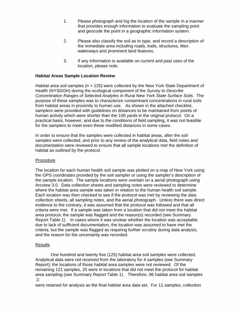
Habitat Area Sampling Protocol, Quality Review, and Data Analysis The habitat area sampling protocol described the process for taking a “habitat area” soil sample as part of the ecological component of the New York State Survey to Describe Concentration Ranges of Selected Analytes in Rural New York State Surface Soils. This appendix provides the definition of habitat and the sampling protocol as originally proposed, as well as a description of the NYSDEC quality review of the sampling locations and analytical data leading to the selection of a final habitat area data set for establishing rural soil concentrations for habitat areas. Habitat Area Concept The ecological component of the survey was designed to measure contaminant concentrations in rural soils that are only marginally influenced by human activity. For purposes of this survey, the concept of habitat is simply a vegetated area which is outside the sphere of regular human activity, is largely undisturbed and provides an area for plants and animals to live, grow, forage, make a nest or burrow etc. A habitat area is a natural landscape rather than a managed one. Therefore, any areas where native soils and vegetation have been significantly altered or disturbed are not considered “only marginally influenced”. Likewise, any areas that have been chemically treated or are specifically managed to exclude biota by practices such as pesticide spraying and herbicide treatments are not considered appropriate for habitat area sampling. Examples of natural landscapes include woodlands, meadows, untreated pastureland, fallow fields, streambanks, wetlands, shrubby areas, and successional fields. While agricultural fields may provide habitat, active agricultural fields are not considered appropriate for habitat area sampling due to the alteration of the soil and the use of fertilizers, herbicides and/or pesticides. Characteristics of a Habitat Area Sample This sample will contain the uppermost six inches of soil immediately below vegetative cover. In the absence of vegetative cover, the sample will contain the uppermost six inches. An appropriate habitat area sampling location should have the characteristics listed on the attached checklist. Selecting the Habitat Area Sample Location After collecting the public health component sample, observe the landscape in the surrounding area to locate the margin of human activity by looking for the transition from the managed to the natural landscape. Select the nearest location that appears to be a habitat area. Proceed to that location and take the sample. While sampling:

31

1. Please photograph and log the location of the sample in a manner that provides enough information to evaluate the sampling point and geocode the point in a geographic information system.

2. Please also classify the soil as to type, and record a description of

the immediate area including roads, trails, structures, litter, waterways and prominent land features.

3. If any information is available on current and past uses of the

location, please note. Habitat Areas Sample Location Review Habitat area soil samples (n = 125) were collected by the New York State Department of Health (NYSDOH) during the ecological component of the Survey to Describe Concentration Ranges of Selected Analytes in Rural New York State Surface Soils. The purpose of these samples was to characterize contaminant concentrations in rural soils from habitat areas in proximity to human use. As shown in the attached checklist, samplers were provided with guidelines on distances to be maintained from points of human activity which were shorter than the 100 yards in the original protocol. On a practical basis, however, and due to the conditions of field sampling, it was not feasible for the samplers to meet even these modified distances in some cases. In order to ensure that the samples were collected in habitat areas, after the soil samples were collected, and prior to any review of the analytical data, field notes and documentation were reviewed to ensure that all sample locations met the definition of habitat as outlined by the protocol. Procedure The location for each human health soil sample was plotted on a map of New York using the GPS coordinates provided by the soil sampler or using the sampler’s description of the sample location. The sample locations were overlain on a aerial photograph using Arcview 3.0. Data collection sheets and sampling notes were reviewed to determine where the habitat area sample was taken in relation to the human health soil sample. Each location was then checked to see if the protocol was met by reviewing the data collection sheets, all sampling notes, and the aerial photograph. Unless there was direct evidence to the contrary, it was assumed that the protocol was followed and that all criteria were met. If a sample was taken from a location that did not meet the habitat area protocol, the sample was flagged and the reason(s) recorded (see Summary Report Table 1). In cases where it was unclear whether the location was acceptable due to lack of sufficient documentation, the location was assumed to have met the criteria, but the sample was flagged as requiring further scrutiny during data analysis, and the reason for the uncertainty was recorded. Results One hundred and twenty five (125) habitat area soil samples were collected. Analytical data were not received from the laboratory for 4 samples (see Summary Report); the locations of those habitat area samples were not reviewed. Of the remaining 121 samples, 25 were in locations that did not meet the protocol for habitat area sampling (see Summary Report Table 1). Therefore, 96 habitat area soil samples

were retained for analysis as the final habitat area data set. For 11 samples, collection

32

photographs, sampling notes, or the aerial photograph indicated that the sample was taken from a location of questionable habitat characteristics, however there was no definitive data to indicate that the sample should be removed from the habitat area dataset. These samples were flagged as deserving additional scrutiny during data analysis. Data Quality Review Data were received for 24 inorganics, 61 volatile organic compounds (VOCs), 55 semi- volatile organic compounds (SVOCs), 17 pesticides, and 7 PCB Aroclors. For one sample, data for all SVOCs were missing from the laboratory report. All lab qualified data were retained for analysis. Several analytes were considered lab contaminants and those data were removed from the habitat area dataset. (see Summary Report). Data Analysis Descriptive statistics (number of detections, minimum and maximum detection, median, and various percentiles) were calculated for all analytes detected in at least 10% of the samples. For analytes with fewer than 10% detections in this statewide survey, the detection of the analyte was considered too rare an event to legitimately calculate a statewide rural soil background concentration for habitat areas. The final habitat area data set contained 21 inorganics, 1 VOC, and 2 SVOCs with sufficient number of detections for establishing a background value for habitat areas (Table D-1).

80

Table 1. Results of protocol conformance and missing data evaluations.

SampleNumber

Reason for Elimination or Absence Source of Determination

35D Owner stated property was formerly an orchard. Protocol prohibited sampling at orchards.

sampling notes

56D Data not received from the lab60D Data not received from the lab65D Data not received from the lab70D Data not received from the lab75D Data not received from the lab

101D Owner stated property was formerly an orchard. Protocol prohibited sampling at orchards.

sampling notes

SampleNumber


16N Data not received from the lab56N Data not received from the lab75N Data not received from the lab

SampleNumber


5H Sample located in lawn collection photograph sampling notes

26H Sample taken in treed area surrounded by active agriculture and not large enough to meet habitatrequirement

aerial photograph sampling notes

27H Sample taken in residential area surrounded by active agriculture, no habitat area

aerial photograph sampling notes

29H Sample taken within active lawn area at the edge of habitat area

sampling notes

30H Sample taken in treed area surrounded by residential area and active agricultural, no habitat area available on property

sampling notesaerial photograph

31H Sample taken in hedgerow at the edge of property, no habitat area available on property

sampling notes

SOURCE-DISTANT DATA SET

NEAR SOURCE DATA SET

HABITAT DATA SET

81

SampleNumber


34H Sample taken in active agriculture field aerial photograph sampling notes

35H Sample taken on a property that was a converted orchard, no habitat area available on property

sampling notes

37H Sample taken in recently active agriculture field sampling notesaerial photograph

41H No habitat area available on property sampling notesaerial photograph

42H Sample taken on a residential property surrounded by active agriculture, no habitat area available


43H No habitat area available on property and no sampling data collected

aerial photograph

59H No habitat area available on property sampling notesaerial photograph

60H Data not received from the lab65H Data not received from the lab70H Data not received from the lab75H Data not received from the lab79H No habitat area available on property sampling notes

aerial photograph81H Sample taken within active agriculture field on the edge

of habitat areascollection photograph sampling notes

85H Sample taken in area too close to active agriculture sampling notesaerial photograph

87H Sample taken in area of active agriculture sampling notesaerial photograph

88H Sample taken in hedgerow between active agriculture fieldsampling notes90H Sample taken in active agricultural field, no habitat area

available on propertysampling notesaerial photograph

93H Sample taken in close proximity to active agriculture sampling notesaerial photograph

101H Sample taken in area that was converted orchard sampling notes106H Sample taken in active agricultural field sampling notes114H Sample taken in active agriculture field collection photograph

sampling notes115H Sample taken in recently active agriculture field sampling notes

124H Sample taken in area that is managed either for agriculture or recreational area


HABITAT DATA SET (continued)

82

Table 2. Counties where rural soil samples were collected (by sample type). County Source-distant Near source Habitat Total Albany 1 0 1 2 Alleganey 1 0 1 2 Broome 1 0 1 2 Cattaraugus 3 0 2 5 Cayuga 1 0 1 2 Chautauqua 3 1 1 5 Chenango 3 1 3 7 Clinton 3 0 3 6 Columbia 1 0 2 3 Cortland 4 1 3 8 Delaware 3 2 3 8 Dutchess 6 1 5 12 Erie 3 0 3 6 Essex 4 2 3 9 Franklin 5 3 5 13 Fulton 2 1 2 5 Genessee 3 1 1 5 Greene 2 0 2 4 Hamilton 2 0 2 4 Herkimer 4 2 3 9 Jefferson 2 0 1 3 Lewis 4 1 4 9 Livingston 3 1 2 6 Madison 1 0 0 1 Montgomery 1 1 0 2 Niagara 2 0 0 2 Oneida 1 0 0 1 Orange 1 0 1 2 Orleans 2 1 1 4 Oswego 2 1 2 5 Otsego 5 1 5 11 Putnam 1 0 1 2 Rensselaer 2 1 2 5 Saratoga 3 0 3 6 Schoharie 2 0 1 3 Schuyler 2 0 0 2 Seneca 1 0 0 1 St. Lawrence 9 0 9 18 Steuben 3 2 3 8 Sullivan 4 0 4 8 Tioga 4 2 3 9 Tompkins 1 0 1 2 Ulster 1 1 1 3 Warren 3 1 3 7 Washington 2 0 2 4 Wyoming 1 0 0 1 TOTAL 118 28 96 242

83

Table 3. Average (mean) relative percent differences for field duplicate samples of selected PAHs and metals.

Sample Pair Alu

min

um

Ars

enic

Bar

ium

Ber

ylliu

m

Cad

miu

m

Cal

cium

Chr

omiu

m (T

otal

)C

obal

tC

oppe

rIro

nLe

adM

agne

sium

Man

gane

seM

ercu

ryN

icke

lPo

tass

ium

Sele

nium

Sodi

umVa

nadi

umZi

ncB

enzo

(a)a

nthr

acen

e

Ben

zo(a

)pyr

ene

Ben

zo(b

)fluo

rant

hene

Ben

zo(g

,h,i)

pery

lene

Ben

zo(k

)fluo

rant

hene

2D, 2DD 3 6 2 2 8 19 47 1 6 36 2 15 0 43 22 29 34 23H, 3HD 3 27 5 22 15 41 37 22 0 24 2 22 31 14 26 66 45N, 5ND 22 28 22 7 39 20 12 25 32 1 14 32 0 12 26 77 4 26 99H, 9HD 65 15 44 34 67 22 28 60 13 75 71 46 86 46 46 5 1610D, 10DD 12 93 10 15 27 15 11 6 14 6 8 20 2 0 13 11 21 3 8 2520D, 20DD 15 9 6 6 14 4 10 15 11 15 30 19 3 15 10 5 26 0 9 6 9 9 21 7 229H, 29HD 18 60 10 10 22 12 13 12 8 12 9 10 8 22 12 28 5 16 12 1530D, 30DD 1 2 0 6 1 1 2 3 2 0 0 4 11 13 3 3 25 17 1 239H, 39HD 5 15 1 10 33 19 3 17 10 8 20 0 24 24 5 4 25 3 240D, 40DD 10 12 10 15 32 8 8 13 8 10 12 9 13 0 7 8 32 12 8 849H, 49HD 3 20 0 5 11 25 0 12 7 5 10 5 19 22 4 13 13 23 0 150D, 50DD 2 10 5 8 3 6 3 15 4 8 7 5 28 67 2 6 11 40 8 559H, 59HD 3 18 6 3 11 6 1 1 5 0 1 3 2 29 2 7 4 1 679H, 79HD 2 10 5 6 29 4 5 5 7 0 4 2 2 0 17 6 9 71 4 080D, 80DD 3 7 1 3 19 0 2 1 1 2 1 0 11 15 4 10 5 0 2 389H, 89HD 8 6 7 4 19 30 7 14 5 9 4 12 3 5 12 7 19 1 190D, 90DD 1 1 4 4 41 9 4 17 6 11 10 11 17 67 6 12 10 2 2 1100D, 100DD 2 18 6 8 7 0 1 11 4 6 12 4 22 0 1 14 22 42 1 4 20 25109H, 109HD 4 20 56 6 10 22 49 2 24 5 11 24 0 23 10 39 18 17 9110D, 110DD 34 20 7 31 90 3 36 21 36 15 2 58 42 40 66 17 22 63 11 10119H, 119HD 19 2 9 9 26 8 13 10 0 9 8 11 10 25 9 10 24 14 9120D, 120DD 1 3 2 5 2 17 10 23 12 1 4 4 11 29 27 20 12 11 9123N, 123ND 12 33 17 29 16 33 5 6 0 5 12 8 15 33 6 27 40 18 18 8125N, 125ND 21 5 26 65 26 1 7 20 4 2 24 2 40 22 4 100 5 8 2N 24 20 24 24 20 24 24 24 24 24 24 24 24 24 24 24 24 16 24 24 1 2 2 1 1Mean RPD 11 19 10 11 24 14 11 16 11 11 9 14 16 21 18 14 27 21 11 7 9 15 23 7 2

NOTE: Only pairs for which both the sample and the duplicate had detected values were used in this analysis. Bold type indicates RPDs that are above the QAPP criterion of +/- 50 percent.

METALS PAHs

84

Table 4. Representation of rural New York State soil orders in the Rural Survey database (Rural Survey, 2005).

Soil Order

Percentage of NYS

Percentage of Rural NYS

Percentage of Source-Distant

Samples (n=120)

Percentage of Remote Samples (n=121)

Percentage of Near Source

Samples (n=28)

Alfisols 20% 20% 22% 22% 18% Entisols 1.8% 1.4% 0% 0% 0% Histosols 1.7% 1.8% 0% 0% 0% Inceptisols 48% 49% 55% 55% 57% Mollisols 0% 0% 0% 0% 0% Spodosols 22% 24% 23% 22% 25% Utilisols 0.8% 0.8% 0% 0% 0% Unknown 5.7% 3% 1% 1% 0%

85

Table 5a. MDL ranges for analytes not detected in the source-distant data set.

Organics (ppb)

ANALYTE N MIN MAX ANALYTE N MIN MAXAldrin 118 1.1 5.0 Chloroethane 118 0.6 2.5Aroclor-1221 118 3.6 17.0 Chloromethane 118 0.3 1.6Aroclor-1232 118 2.5 11.0 4-Chloro-3-methylphenol 118 10 47Aroclor-1242 118 3.2 15.0 2-Chloronaphthalene 118 7 33Aroclor-1248 118 3.7 17.0 2-Chlorophenol 118 15 68Aroclor-1254 118 1.4 6.3 4-Chlorophenyl-phenylether 118 9 39Aroclor-1260 118 3.0 14.0 4,4-DDE 118 1.3 6.1Benzene 118 0.21 0.96 4,4-DDT 118 1.9 8.8alpha-BHC 118 1.1 5.3 Dibromochloromethane 118 0.3 1.4beta-BHC 118 1.2 5.4 1,2-Dibromo-3-Chloropropane 118 0.7 3.2delta-BHC 39 0.4 4.2 1,2-Dibromoethane 118 0.4 2.0gamma-BHC 118 1.2 5.8 1,2-Dichlorobenzene 118 0.4 1.9bis(2-Chloroethoxy)methane 118 16 72 1,3-Dichlorobenzene 118 0.2 1.0bis(2-Chloroethyl)ether 118 17 78 1,4-Dichlorobenzene 118 0.4 1.7Bromochloromethane 118 0.5 2.1 3,3-Dichlorobenzidine 118 55 340Bromoform 118 0.3 1.4 Dichlorodifluoromethane 118 1.3 5.9Bromomethane 118 0.7 3.4 1,1-Dichloroethane 118 0.4 1.74-Bromophenyl-phenylether 118 9 41 1,2-Dichloroethane 118 3.2 15.0Tert butyl alcohol 118 15 70 1,1-Dichloroethene 118 0.2 1.0sec-Butylbenzene 118 0.3 1.1 cis-1,2-Dichloroethene 118 0.4 1.7tert-Butylbenzene 118 0.3 1.3 trans-1,2-Dichloroethene 118 0.4 1.8Carbon Disulfide 118 0.11 0.48 2,4-Dichlorophenol 118 12 55Carbon Tetrachloride 118 0.3 1.4 1,2-Dichloropropane 118 0.4 1.64-Chloroaniline 118 130 580 cis-1,3-Dichloropropene 118 0.20 0.92Chlorobenzene 118 0.4 1.7 t-1,3-Dichloropropene 118 0.3 1.2

86

ANALYTE N MIN MAX ANALYTE N MIN MAXDieldrin 118 1.0 4.8 4-Nitroaniline 118 27 120Diethylphthalate 118 11 49 Nitrobenzene 118 17 802,4-Dimethylphenol 118 18 85 2-Nitrophenol 118 14 63Dimethylphthalate 118 8 38 4-Nitrophenol 118 33 1504,6-Dinitro-2-methylphenol 118 20 91 N-Nitrosodiphenylamine 118 9 402,4-Dinitrophenol 118 15 69 N-Nitroso-di-n-propylamine 118 15 692,4-Dinitrotoluene 118 7 31 2,2-oxybis(1-Chloropropane) 118 18 852,6-Dinitrotoluene 118 15 67 Pentachlorophenol 118 11 49Endosulfan II 118 1.4 6.3 Styrene 118 0.3 1.5Endosulfan Sulfate 118 1.5 7.1 1,1,2,2-Tetrachloroethane 118 0.6 2.5Endrin 118 1.9 8.7 Toxaphene 118 3.1 14.0Endrin aldehyde 118 1.6 7.3 1,1,1-Trichloroethane 118 0.3 1.3Endrin ketone 118 1.3 6.2 1,1,2-Trichloroethane 118 0.5 2.4Ethyl Benzene 118 0.3 1.2 Trichloroethene 118 0.3 1.5Heptachlor 118 1.3 6.3 2,4,5-Trichlorophenol 118 23 100Hexachlorobenzene 118 6 30 2,4,6-Trichlorophenol 118 12 57Hexachlorobutadiene 118 12 55 1,1,2-Trichlorotrifluoroethane 118 0.5 2.2Hexachlorocyclopentadiene 118 9 39 1,2,4-Trimethylbenzene 118 0.4 1.9Hexachloroethane 118 16 75 1,3,5-Trimethylbenzene 118 0.3 1.42-Hexanone 118 3.3 15.0 Vinyl Chloride 118 0.2 1.1Isophorone 118 13 59 Total Endrins NA 4.8 22.2Isopropylbenzene 118 0.4 1.8Methoxychlor 118 1.3 6.0 Inorganics (ppm)Methyl tert-butyl Ether 118 0.2 1.1Methyl Acetate 118 1.3 6.1 ANALYTE N MIN MAXMethylcyclohexane 118 0.2 1.7 Cyanide 118 0.1 2.44-Methyl-2-Pentanone 118 2.5 11.0 Cyanide-Amenable 118 0.5 2.42-Nitroaniline 118 12 57 Thallium 118 0.0 1.63-Nitroaniline 118 55 250 NA= Not applicable.

87

gamma-Chlordane 96 1.6 7.0 trans-1,2-Dichloroethene 96 0.4 1.8

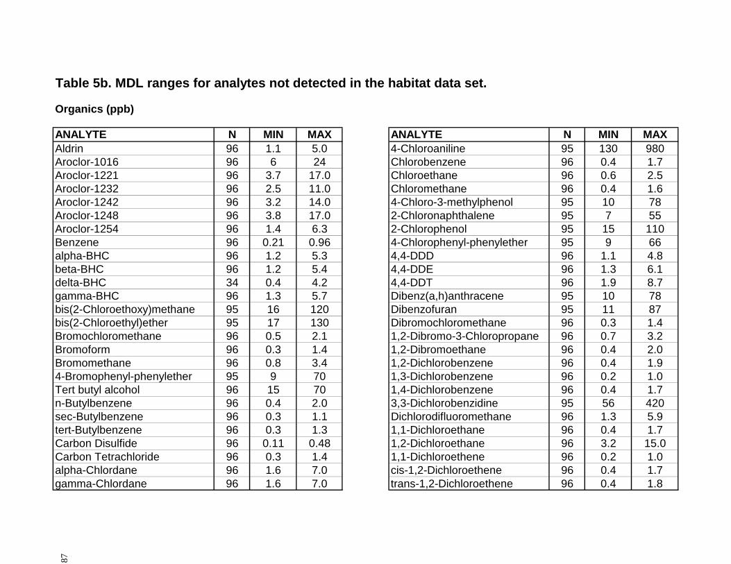
Table 5b. MDL ranges for analytes not detected in the habitat data set.

Organics (ppb)

ANALYTE N MIN MAX ANALYTE N MIN MAXAldrin 96 1.1 5.0 4-Chloroaniline 95 130 980Aroclor-1016 96 6 24 Chlorobenzene 96 0.4 1.7Aroclor-1221 96 3.7 17.0 Chloroethane 96 0.6 2.5Aroclor-1232 96 2.5 11.0 Chloromethane 96 0.4 1.6Aroclor-1242 96 3.2 14.0 4-Chloro-3-methylphenol 95 10 78Aroclor-1248 96 3.8 17.0 2-Chloronaphthalene 95 7 55Aroclor-1254 96 1.4 6.3 2-Chlorophenol 95 15 110Benzene 96 0.21 0.96 4-Chlorophenyl-phenylether 95 9 66alpha-BHC 96 1.2 5.3 4,4-DDD 96 1.1 4.8beta-BHC 96 1.2 5.4 4,4-DDE 96 1.3 6.1delta-BHC 34 0.4 4.2 4,4-DDT 96 1.9 8.7gamma-BHC 96 1.3 5.7 Dibenz(a,h)anthracene 95 10 78bis(2-Chloroethoxy)methane 95 16 120 Dibenzofuran 95 11 87bis(2-Chloroethyl)ether 95 17 130 Dibromochloromethane 96 0.3 1.4Bromochloromethane 96 0.5 2.1 1,2-Dibromo-3-Chloropropane 96 0.7 3.2Bromoform 96 0.3 1.4 1,2-Dibromoethane 96 0.4 2.0Bromomethane 96 0.8 3.4 1,2-Dichlorobenzene 96 0.4 1.94-Bromophenyl-phenylether 95 9 70 1,3-Dichlorobenzene 96 0.2 1.0Tert butyl alcohol 96 15 70 1,4-Dichlorobenzene 96 0.4 1.7n-Butylbenzene 96 0.4 2.0 3,3-Dichlorobenzidine 95 56 420sec-Butylbenzene 96 0.3 1.1 Dichlorodifluoromethane 96 1.3 5.9tert-Butylbenzene 96 0.3 1.3 1,1-Dichloroethane 96 0.4 1.7Carbon Disulfide 96 0.11 0.48 1,2-Dichloroethane 96 3.2 15.0Carbon Tetrachloride 96 0.3 1.4 1,1-Dichloroethene 96 0.2 1.0alpha-Chlordane 96 1.6 7.0 cis-1,2-Dichloroethene 96 0.4 1.7

88

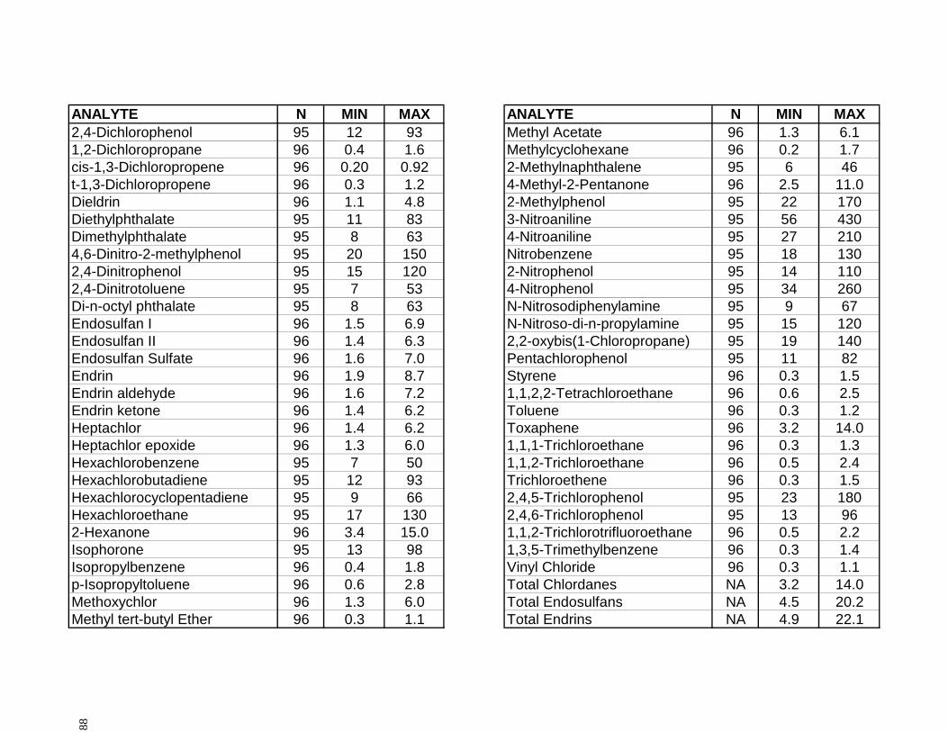
ANALYTE N MIN MAX ANALYTE N MIN MAX2,4-Dichlorophenol 95 12 93 Methyl Acetate 96 1.3 6.11,2-Dichloropropane 96 0.4 1.6 Methylcyclohexane 96 0.2 1.7cis-1,3-Dichloropropene 96 0.20 0.92 2-Methylnaphthalene 95 6 46t-1,3-Dichloropropene 96 0.3 1.2 4-Methyl-2-Pentanone 96 2.5 11.0Dieldrin 96 1.1 4.8 2-Methylphenol 95 22 170Diethylphthalate 95 11 83 3-Nitroaniline 95 56 430Dimethylphthalate 95 8 63 4-Nitroaniline 95 27 2104,6-Dinitro-2-methylphenol 95 20 150 Nitrobenzene 95 18 1302,4-Dinitrophenol 95 15 120 2-Nitrophenol 95 14 1102,4-Dinitrotoluene 95 7 53 4-Nitrophenol 95 34 260Di-n-octyl phthalate 95 8 63 N-Nitrosodiphenylamine 95 9 67Endosulfan I 96 1.5 6.9 N-Nitroso-di-n-propylamine 95 15 120Endosulfan II 96 1.4 6.3 2,2-oxybis(1-Chloropropane) 95 19 140Endosulfan Sulfate 96 1.6 7.0 Pentachlorophenol 95 11 82Endrin 96 1.9 8.7 Styrene 96 0.3 1.5Endrin aldehyde 96 1.6 7.2 1,1,2,2-Tetrachloroethane 96 0.6 2.5Endrin ketone 96 1.4 6.2 Toluene 96 0.3 1.2Heptachlor 96 1.4 6.2 Toxaphene 96 3.2 14.0Heptachlor epoxide 96 1.3 6.0 1,1,1-Trichloroethane 96 0.3 1.3Hexachlorobenzene 95 7 50 1,1,2-Trichloroethane 96 0.5 2.4Hexachlorobutadiene 95 12 93 Trichloroethene 96 0.3 1.5Hexachlorocyclopentadiene 95 9 66 2,4,5-Trichlorophenol 95 23 180Hexachloroethane 95 17 130 2,4,6-Trichlorophenol 95 13 962-Hexanone 96 3.4 15.0 1,1,2-Trichlorotrifluoroethane 96 0.5 2.2Isophorone 95 13 98 1,3,5-Trimethylbenzene 96 0.3 1.4Isopropylbenzene 96 0.4 1.8 Vinyl Chloride 96 0.3 1.1p-Isopropyltoluene 96 0.6 2.8 Total Chlordanes NA 3.2 14.0Methoxychlor 96 1.3 6.0 Total Endosulfans NA 4.5 20.2Methyl tert-butyl Ether 96 0.3 1.1 Total Endrins NA 4.9 22.1

89

Inorganics (ppm)

ANALYTE N MIN MAXCyanide 96 0.1 2.4Cyanide-Amenable 96 0.5 2.4Thallium 96 0.3 1.6

NA= Not applicable.

90

Table 5c. MDL ranges for analytes not detected in the near source data set.

Chlorobenzene 28 0.4 0.9 t-1,3-Dichloropropene 28 0.29 0.66

Organics (ppb)

ANALYTE N MIN MAX ANALYTE N MIN MAXAldrin 28 1.2 2.7 Chloroethane 28 0.6 1.3Aroclor-1016 28 5.9 13.0 Chloromethane 28 0.38 0.85Aroclor-1221 28 4.0 9.0 4-Chloro-3-methylphenol 28 11 110Aroclor-1232 28 2.7 6.1 2-Chloronaphthalene 28 8 80Aroclor-1242 28 3.5 7.8 2-Chlorophenol 28 16 170Aroclor-1248 28 4.1 9.3 4-Chlorophenyl-phenylether 28 9 95Aroclor-1254 28 1.5 3.4 4,4-DDD 28 1.1 2.6Benzene 28 0.23 0.52 4,4-DDE 28 1.4 3.3alpha-BHC 28 1.2 2.8 4,4-DDT 28 2.1 4.7beta-BHC 28 1.3 2.9 Dibenz(a,h)anthracene 28 11 110delta-BHC 10 0.4 2.2 Dibromochloromethane 28 0.33 0.75gamma-BHC 28 1.4 3.1 1,2-Dibromo-3-Chloropropane 28 0.8 1.7bis(2-Chloroethoxy)methane 28 17 170 1,2-Dibromoethane 28 0.5 1.1bis(2-Chloroethyl)ether 28 18 190 1,2-Dichlorobenzene 28 0.5 1.0Bromochloromethane 28 0.5 1.1 1,3-Dichlorobenzene 28 0.24 0.54Bromoform 28 0.34 0.77 1,4-Dichlorobenzene 28 0.40 0.90Bromomethane 28 0.8 1.8 3,3-Dichlorobenzidine 28 59 6204-Bromophenyl-phenylether 28 10 100 Dichlorodifluoromethane 28 1.4 3.2Tert butyl alcohol 28 17 37 1,1-Dichloroethane 28 0.40 0.91sec-Butylbenzene 28 0.27 0.62 1,2-Dichloroethane 28 3.5 7.9tert-Butylbenzene 28 0.31 0.71 1,1-Dichloroethene 28 0.24 0.55Carbon Disulfide 28 0.11 0.26 cis-1,2-Dichloroethene 28 0.40 0.90Carbon Tetrachloride 28 0.34 0.76 trans-1,2-Dichloroethene 28 0.42 0.95alpha-Chlordane 28 1.7 3.8 2,4-Dichlorophenol 28 13 130gamma-Chlordane 28 1.7 3.8 1,2-Dichloropropane 28 0.38 0.864-Chloroaniline 28 140 1,400 cis-1,3-Dichloropropene 28 0.22 0.50

91

2-Methylphenol 28 23 240

ANALYTE N MIN MAX ANALYTE N MIN MAXDieldrin 28 1.1 2.6 2-Nitroaniline 28 13 1402,4-Dimethylphenol 28 20 210 3-Nitroaniline 28 60 6204,6-Dinitro-2-methylphenol 28 21 220 4-Nitroaniline 28 29 3002,4-Dinitrophenol 28 16 170 Nitrobenzene 28 19 1902,4-Dinitrotoluene 28 7 76 2-Nitrophenol 28 15 1502,6-Dinitrotoluene 28 16 160 4-Nitrophenol 28 36 370Di-n-octyl phthalate 28 9 92 N-Nitrosodiphenylamine 28 9 97Endosulfan I 28 1.6 3.7 N-Nitroso-di-n-propylamine 28 16 170Endosulfan II 28 1.5 3.4 2,2-oxybis(1-Chloropropane) 28 20 210Endosulfan Sulfate 28 1.7 3.8 Pentachlorophenol 28 12 120Endrin 28 2.0 4.6 Styrene 28 0.36 0.80Endrin aldehyde 28 1.7 3.9 1,1,2,2-Tetrachloroethane 28 0.6 1.4Endrin ketone 28 1.5 3.3 Toluene 28 0.29 0.66Ethyl Benzene 28 0.28 0.64 Toxaphene 28 3.4 7.6Heptachlor 28 1.5 3.3 1,1,1-Trichloroethane 28 0.31 0.69Heptachlor epoxide 28 1.4 3.2 1,1,2-Trichloroethane 28 0.6 1.3Hexachlorobenzene 28 7 72 Trichloroethene 28 0.36 0.82Hexachlorobutadiene 28 13 130 2,4,5-Trichlorophenol 28 24 250Hexachlorocyclopentadiene 28 9 96 2,4,6-Trichlorophenol 28 13 140Hexachloroethane 28 18 180 1,1,2-Trichlorotrifluoroethane 28 0.5 1.22-Hexanone 28 3.6 8.2 1,3,5-Trimethylbenzene 28 0.32 0.73Isophorone 28 14 140 Vinyl Chloride 28 0.27 0.60Isopropylbenzene 28 0.42 0.95 Total Chlordanes NA 3.4 7.6Methoxychlor 28 1.4 3.2 Total Endosulfans NA 4.8 10.9Methyl tert-butyl Ether 28 0.26 0.59 Total Endrins NA 5.2 11.8Methyl Acetate 28 1.4 3.3Methylcyclohexane 28 0.26 0.912-Methylnaphthalene 28 6 664-Methyl-2-Pentanone 28 2.7 6.2

92

Inorganics (ppm)

ANALYTE N MIN MAXAntimony 28 0.6 1.5Cyanide 28 0.1 1.3Cyanide-Amenable 28 0.6 1.3Thallium 28 0.37 0.85

NA= Not applicable.

93

Indeno(1,2,3-cd)pyrene 118 5.9 <8 <10 <11 <14 <34 76 180 1,400

Table 6a. Distribution-free percentile values for detected analytes in the source-distant data set (outliers included).

Organics (ppb)

ANALYTE N % MIN MAX25 50 75 90 95 98

Acenaphthene 118 1.7 <8 <9 <10 <11 <20 <33 <35 110Acenaphthylene 118 4.2 <10 <13 <14 <16 <36 46* 110 590Anthracene 118 6.8 <8 <10 <11 <13 <35 97 120 150Aroclor-1016 118 0.8 <5 <7 <7 <8 <10 <18 <24 72Benzo(a)anthracene 118 10.2 <5 <7 <7 <10 72 160 500 2,600Benzo(a)pyrene 118 10.2 <6 <7 <8 <12 41 120 470 3,400Benzo(b)fluoranthene 118 13.6 <18 <23 <26 <38 110 360 590 4,600Benzo(k)fluoranthene 118 10.2 <12 <15 <16 <23 <54*** 100 330 1,700Benzo(g,h,i)perylene 118 7.6 <15 <19 <21 <25 <62*** 70 200 1,500n-Butylbenzene 118 2.5 <0.4 <0.5 <0.6 <0.6 <0.9 <1.9 2.1 5.6Carbazole 118 4.2 <8 <9 <10 <12 <26 <35 80 150gamma-Chlordane 118 0.8 <1.5 <1.9 <2.0 <2.2 <2.8 5.1* <6.7 <7.1alpha-Chlordane 118 0.8 <1.5 <1.8 <2.0 <2.2 <2.7 <5.2 <7.0 10.0Chrysene 118 12.7 <11 <14 <15 <23 100 230 610 2,4004,4-DDD 118 0.8 <1.0 <1.3 <1.4 <1.5 <1.9 <3.6 <4.9 8.3Dibenz(a,h)anthracene 118 1.7 <10 <12 <14 <15 <27 <44 <46 230Dibenzofuran 118 2.5 <11 <14 <16 <18 <31 <51 53 93Di-n-octyl phthalate 118 0.8 <8 <10 <11 <12 <22 <34 <37 651,4-Dioxane 117 1.7 <21 <25 <28 <30 <41 79* <91 <95Endosulfan I 118 0.8 <1.5 <1.8 <2.0 <2.2 <2.7 <5.2 <7.0 15.0Fluoranthene 118 21.2 <5 <6 <7 <20 130 630 1,200 1,800Fluorene 118 3.4 <10 <12 <13 <15 <33 <45 87 130Heptachlor epoxide 118 0.8 <1.3 <1.6 <1.8 <1.9 <2.4 4.3* <5.8 <6.1

PERCENTILE VALUES

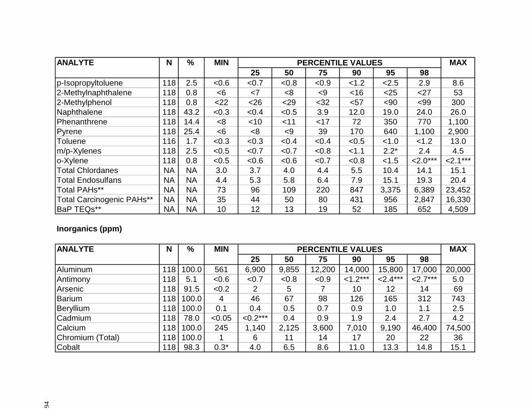
94

ANALYTE N % MIN MAX25 50 75 90 95 98

p-Isopropyltoluene 118 2.5 <0.6 <0.7 <0.8 <0.9 <1.2 <2.5 2.9 8.62-Methylnaphthalene 118 0.8 <6 <7 <8 <9 <16 <25 <27 532-Methylphenol 118 0.8 <22 <26 <29 <32 <57 <90 <99 300Naphthalene 118 43.2 <0.3 <0.4 <0.5 3.9 12.0 19.0 24.0 26.0Phenanthrene 118 14.4 <8 <10 <11 <17 72 350 770 1,100Pyrene 118 25.4 <6 <8 <9 39 170 640 1,100 2,900Toluene 116 1.7 <0.3 <0.3 <0.4 <0.4 <0.5 <1.0 <1.2 13.0m/p-Xylenes 118 2.5 <0.5 <0.7 <0.7 <0.8 <1.1 2.2* 2.4 4.5o-Xylene 118 0.8 <0.5 <0.6 <0.6 <0.7 <0.8 <1.5 <2.0*** <2.1***Total Chlordanes NA NA 3.0 3.7 4.0 4.4 5.5 10.4 14.1 15.1Total Endosulfans NA NA 4.4 5.3 5.8 6.4 7.9 15.1 19.3 20.4Total PAHs** NA NA 73 96 109 220 847 3,375 6,389 23,452Total Carcinogenic PAHs** NA NA 35 44 50 80 431 956 2,847 16,330BaP TEQs** NA NA 10 12 13 19 52 185 652 4,509

Inorganics (ppm)

ANALYTE N % MIN MAX25 50 75 90 95 98

Aluminum 118 100.0 561 6,900 9,855 12,200 14,000 15,800 17,000 20,000Antimony 118 5.1 <0.6 <0.7 <0.8 <0.9 <1.2*** <2.4*** <2.7*** 5.0Arsenic 118 91.5 <0.2 2 5 7 10 12 14 69Barium 118 100.0 4 46 67 98 126 165 312 743Beryllium 118 100.0 0.1 0.4 0.5 0.7 0.9 1.0 1.1 2.5Cadmium 118 78.0 <0.05 <0.2*** 0.4 0.9 1.9 2.4 2.7 4.2Calcium 118 100.0 245 1,140 2,125 3,600 7,010 9,190 46,400 74,500Chromium (Total) 118 100.0 1 6 11 14 17 20 22 36Cobalt 118 98.3 0.3* 4.0 6.5 8.6 11.0 13.3 14.8 15.1

PERCENTILE VALUES

PERCENTILE VALUES

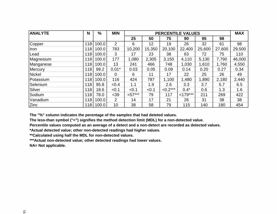
95

ANALYTE N % MIN MAX25 50 75 90 95 98

Copper 118 100.0 2 6 12 19 26 32 61 98Iron 118 100.0 783 10,200 15,350 20,100 22,400 25,600 27,600 29,500Lead 118 100.0 3 17 23 38 63 72 75 110Magnesium 118 100.0 177 1,080 2,305 3,150 4,110 5,130 7,790 46,000Manganese 118 100.0 13 241 466 748 1,030 1,610 1,760 4,550Mercury 118 99.2 0.01* 0.03 0.05 0.09 0.14 0.20 0.27 0.34Nickel 118 100.0 0 6 11 17 22 25 26 49Potassium 118 100.0 116 424 787 1,100 1,480 1,890 2,180 2,440Selenium 118 95.8 <0.4 1.1 1.9 2.6 3.3 3.7 5.7 6.5Silver 118 18.6 <0.1 <0.1 <0.1 <0.2*** 0.4* 0.6 1.3 1.6Sodium 118 78.0 <39 <57*** 79 117 <179*** 211 269 422Vanadium 118 100.0 2 14 17 21 26 31 38 38Zinc 118 100.0 10 38 58 79 115 140 180 454

The "%" column indicates the perentage of the samples that had deteted values.The less-than symbol ("<") signifies the method detection limit (MDL) for a non-detected value.Percentile values computed as an average of a detect and a non-detect are recorded as detected values.*Actual detected value; other non-detected readings had higher values.**Calculated using half the MDL for non-detected values.***Actual non-detected value; other detected readings had lower values.NA= Not applicable.

PERCENTILE VALUES

96

(outliers included).

Organics (ppb)

ANALYTE N % MIN MAX25 50 75 90 95 98

Acenaphthene 95 1.1 <7.7 <9.4 <10 <12 <19 <26 <58 120Acenaphthylene 95 1.1 <10 <13 <14 <16 <26 <35 <79 500Anthracene 95 1.1 <8 <10 <11 <13 <21 <28 <63 510Aroclor-1260 96 1.0 <3 <4 <4 <5 <6 <9 <14 47Benzo(a)anthracene 95 5.3 <5 <7 <7 <9 <17 62 150 1,500Benzo(a)pyrene 95 4.2 <6 <7 <8 <10 <18 <46 110 1,100Benzo(b)fluoranthene 95 5.3 <18 <23 <25 <31 <58 96 150 1,300Benzo(k)fluoranthene 95 5.3 <12 <15 <16 <20 <37 66 <90*** 590Benzo(g,h,i)perylene 95 4.2 <15 <19 <20 <25 <46 <68*** <120*** 4002-Butanone 96 1.0 <2 <3 <3 <4 <5 <7 <11 31Carbazole 95 1.1 <8 <9 <10 <12 <19 <26 <58 150Chrysene 95 5.3 <11 <14 <15 <19 <35 71 190 1,9001,4-Dioxane 96 1.0 <21 <26 <28 <31 <39 <50 <71*** <95***2,4-Dimethylphenol 95 1.1 <19 <23 <25 <31 <49 <63 <140 2702,6-Dinitrotoluene 95 1.1 <15 <18 <20 <24 <39 <50 <110 310Ethyl Benzene 96 1.0 <0.3 <0.3 <0.4 <0.4 <0.5 <0.8 <1.0*** <1.2***Fluoranthene 95 13.7 <5 <6 <7 <11 69 87 330 3,200Fluorene 95 1.1 <10 <12 <13 <16 <25 <33 <75 310Indeno(1,2,3-cd)pyrene 95 4.2 <8 <10 <11 <14 <26 54 75 270Naphthalene 96 33.3 <0.3 <0.4 <0.5 5 10 14 18 <45***2-Nitroaniline 95 1.1 <13 <15 <17 <21 <33 <43 62* <96Phenanthrene 95 6.3 <8 <10 <10 <13 <25 75 240 2,700Phenol 95 1.1 <14 <18 <20 <23 <38 <49 <110 170

PERCENTILE VALUES

Table 6b. Distribution-free percentile values for detected analytes in the habitat data set

97

ANALYTE N % MIN MAX25 50 75 90 95 98

Pyrene 95 18.9 <6 <8 <9 <17 76 170 320 4,6001,2,4-Trimethylbenzene 96 1.0 <0.4 <0.5 <0.6 <0.7 <0.8 1.2* <1.6 <1.9m/p-Xylenes 96 3.1 <0.5 <0.7 <0.7 <0.8 <1.1 <2.1 3.6 5.6o-Xylene 96 3.1 <0.5 <0.6 <0.6 <0.7 <0.9 <1.5*** <2.1*** 2.3Total PAHs** NA NA 0 94 109 171 330 667 1,699 19,027Total Carcinogenic PAHs** NA NA 0 44 48 65 112 271 707 6,674BaP TEQs** NA NA 0 12 13 16 30 75 153 1,428

Inorganics (ppm)

ANALYTE N % MIN MAX25 50 75 90 95 98

Aluminum 96 100.0 906 5,950 9,840 12,750 15,100 16,400 21,400 21,800Antimony 96 2.1 <0.6 <0.7 <0.8 <0.9 <1.1 <2.0 3.3 5.8Arsenic 96 89.6 <0.3 1.7 4.2 7.4 11.1 13.0 16.7 28.1Barium 96 100.0 6 37 57 87 129 176 254 278Beryllium 96 100.0 0.1 0.4 0.5 0.7 1.0 1.1 1.3 3.8Cadmium 96 72.9 <0.05 0.1* 0.4 0.8 1.9 2.1 2.8 3.6Calcium 96 100.0 113 743 1,265 2,820 4,810 6,100 14,800 19,800Chromium (Total) 96 100.0 1.3 5.0 10.7 13.5 16.3 19.1 24.3 24.4Cobalt 96 100.0 0.5 3.2 6.0 8.5 11.6 12.8 13.4 16.9Copper 96 100.0 2 6 11 15 25 33 53 101Iron 96 100.0 1,190 8,770 15,050 19,800 24,500 26,200 29,500 29,800Lead 96 100.0 3 17 26 37 54 63 77 112Magnesium 96 100.0 105 954 1,940 2,925 3,920 5,150 7,930 10,100Manganese 96 100.0 17 147 397 650 1,130 1,600 1,940 4,140Mercury 96 100.0 0.01 0.05 0.07 0.10 0.15 0.18 0.28 0.30Nickel 96 100.0 1 4 11 17 22 25 37 50

PERCENTILE VALUES

PERCENTILE VALUES

98

ANALYTE N % MIN MAX25 50 75 90 95 98

Potassium 96 100.0 126 286 599 949 1,310 1,700 2,230 2,440Selenium 96 95.8 0.4* 1.2 2.1 2.6 3.3 3.9 4.4 5.1Silver 96 18.8 <0.1 <0.1 <0.2*** <0.2*** 0.5* 0.7 1.0 1.2Sodium 96 74.0 <39 57* 75* 111* 203 251 282 627Vanadium 96 100.0 3 12 18 23 26 33 39 44Zinc 96 100.0 11 30 51 70 88 109 157 242


PERCENTILE VALUES

99

Pyrene 28 50.0 <7 <8 53* 370 1,600 2,800 8,700 8,700

Table 6c. Distribution-free percentile values for detected analytes in the near source data set (outliers included).

Organics (ppb)

ANALYTE N % MIN MAX25 50 75 90 95 98

Acenaphthene 28 7.1 <8 <9 <10 <19 <85 100 150 150Acenaphthylene 28 10.7 <11 <13 <15 <25 98* <110 500 500Anthracene 28 17.9 <9 <10 <12 <22 180 310 620 620Aroclor-1260 28 7.1 <3 <4 <4 <5 <8 20 32 32Benzo(a)anthracene 28 35.7 <6 <7 <11 210 1,200 1,200 2,900 2,900Benzo(a)pyrene 28 32.1 <7 <7 <10 150 630 1,100 2,400 2,400Benzo(b)fluoranthene 28 42.9 <20 <24 41* 305 850 1,200 3,300 3,300Benzo(k)fluoranthene 28 25.0 <13 <15 <17 160 360 740 1,500 1,500Benzo(g,h,i)perylene 28 21.4 <17 <19 <22 74 290 550 630 630n-Butylbenzene 28 7.1 <0.5 <0.5 <0.5 <0.6 <1.1 2.1 3.4 3.4Carbazole 28 10.7 <8 <9 <11 <19 110 230 680 680Chrysene 28 39.3 <12 <14 <25 210 540 630 1,300 1,300Dibenzofuran 28 7.1 <13 <14 <16 <27 <50*** <130*** 180 180Diethylphthalate 28 3.6 <12 <13 <15 <25 <48 <120 130 130Dimethylphthalate 28 3.6 <9 <10 <11 <20 <36 <92 580 5801,4-Dioxane 28 3.6 <23* <24 <26 <29 <35 <48 <51 <51Fluoranthene 28 46.4 <5 <6 <26 320 2,000 2,800 7,400 7,400Fluorene 28 10.7 <11 <12 <14 <25 120 160 580 580Indeno(1,2,3-cd)pyrene 28 21.4 <9 <10 <12 <57 260 620 660 660p-Isopropyltoluene 28 3.6 <0.7 <0.7 <0.8 <0.9 <1.4 <1.5 14.0 14.0Naphthalene 28 39.3 <0.3 <0.4 <0.5 4.7 15.0 16.0 17.0 17.0Phenanthrene 28 42.9 <9 <10 <19 110 950 1,600 8,500 8,500

PERCENTILE VALUES

101

ANALYTE N % MIN MAX25 50 75 90 95 98

1,2,4-Trimethylbenzene 28 3.6 <0.5 <0.5 <0.5 <0.6 <1.0 <1.0 3.0 3.0m/p-Xylenes 28 7.1 <0.6 <0.6 <0.7 <0.8 <1.3 2.7 6.8 6.8o-Xylene 28 7.1 <0.5 <0.5 <0.6 <0.7 1.0* <1.1 2.4 2.4Total PAHs** NA NA 162 204 358 2,239 9,054 14,554 38,215 38,215Total Carcinogenic PAHs** NA NA 78 93 155 1,212 3,965 6,182 11,114 11,114BaP TEQs** NA NA 21 25 37 274 909 1,433 3,135 3,135

Inorganics (ppm)

ANALYTE N % MIN MAX25 50 75 90 95 98

Aluminum 28 100.0 1,860 5,235 8,550 11,500 13,700 13,700 14,400 14,400Arsenic 28 96.4 <0.3 2.3 3.2 6.9 8.0 12.8 14.1 14.1Barium 28 100.0 11 32 63 78 156 156 188 188Beryllium 28 100.0 0.2 0.4 0.4 0.6 0.9 1.0 1.3 1.3Cadmium 28 75.0 <0.1 <0.1*** 0.4 0.7 1.5 2.1 2.3 2.3Calcium 28 100.0 465 2,030 3,300 6,925 38,800 53,900 56,500 56,500Chromium (Total) 28 100.0 1.3 5.8 11.1 14.6 15.8 16.0 17.5 17.5Cobalt 28 96.4 <0.2 3.7 5.6 9.3 13.2 13.4 24.1 24.1Copper 28 100.0 3.4 8.6 15.5 19.4 23.9 25.9 29.6 29.6Iron 28 100.0 3,090 10,030 13,300 19,550 22,800 23,200 25,700 25,700Lead 28 100.0 9 17 26 48 61 84 133 133Magnesium 28 100.0 220 1,345 2,680 3,415 6,480 13,700 31,400 31,400Manganese 28 100.0 17 236 426 690 1,160 1,290 1,560 1,560Mercury 28 96.4 <0.01 0.03 0.04 0.07 0.14 0.19 0.28 0.28Nickel 28 100.0 1.2 5.2 11.2 17.2 22.3 24.9 29.5 29.5Potassium 28 100.0 122 510 800 1,150 1,460 1,560 1,660 1,660

PERCENTILE VALUES

PERCENTILE VALUES

ANALYTE N % MIN MAX25 50 75 90 95 98

Selenium 28 89.3 <0.4 1.1 1.7 2.5 3.5 4.2 4.4 4.4Silver 28 17.9 <0.12 <0.13 <0.14 <0.18*** <0.27*** 0.37 0.40 0.40Sodium 28 92.9 53* 100 131 185 221 295 806 806Vanadium 28 100.0 4.0 10.8 15.3 18.6 21.4 22.7 25.9 25.9Zinc 28 100.0 15 43 58 73 91 107 109 109


PERCENTILE VALUES

102

Table D-1. Final data set for analytes detected in habitat areas.

Organics (ppb) ANALYTE N % MIN PERCENTILE VALUES MAX 25 50 75 90 95 98 Fluoranthene 95 13.7 <DL <DL <DL <DL 69 87 330 3200 Naphthalene 96 33.3 <DL <DL <DL 5 10 14 18 1 Pyrene 95 18.9 <DL <DL <DL <DL 76 170 320 4600 Inorganics (ppm) ANALYTE N % MIN PERCENTILE VALUES MAX 25 50 75 90 95 98 Aluminum 96 100.0 906 5950 9840 12750 15100 16400 21400 21800 Arsenic 96 89.6 <DL 1.7 4.2 7.4 11.1 13.0 16.7 28.1 Barium 96 100.0 6 37 57 87 129 176 254 278 Beryllium 96 100.0 0.1 0.4 0.5 0.7 1.0 1.1 1.3 3.8 Cadmium 96 72.9 <DL 0.1 0.4 0.8 1.9 2.1 2.8 3.6 Calcium 96 100.0 113 743 1265 2820 4810 6100 14800 19800 Chromium (Total) 96 100.0 1.3 5.0 10.7 13.5 16.3 19.1 24.3 24.4 Cobalt 96 100.0 0.5 3.2 6.0 8.5 11.6 12.8 13.4 16.9 Copper 96 100.0 2 6 11 15 25 33 53 101 Iron 96 100.0 1190 8770 15050 19800 24500 26200 29500 29800 Lead 96 100.0 3 17 26 37 54 63 77 112

103

Magnesium 96 100.0 105 954 1940 2925 3920 5150 7930 10100 Manganese 96 100.0 17 147 397 650 1130 1600 1940 4140 Mercury 96 100.0 0.01 0.05 0.07 0.10 0.15 0.18 0.28 0.30 Nickel 96 100.0 1 4 11 17 22 25 37 50 Potassium 96 100.0 126 286 599 949 1310 1700 2230 2440 ANALYTE N % MIN PERCENTILE VALUES MAX 25 50 75 90 95 98 Selenium 96 95.8 0.4 1.2 2.1 2.6 3.3 3.9 4.4 5.1 Silver 96 18.8 <DL <DL <DL <DL 0.5 0.7 1.0 1.2 Sodium 96 74.0 <DL 57 75 111 203 251 282 627 Vanadium 96 100.0 3 12 18 23 26 33 39 44 Zinc 96 100.0 11 30 51 70 88 109 157 242 The "%" column indicates the percentage of the samples that had detected values. <DL = less than detection limit; not detected

104

Appendix E

Approaches for Modifying SCOs for a Track 3 Cleanup or Developing SCOs for

Contaminants Not Included in the Track 1 or 2 Tables

This Appendix is a brief guide to the resources in the Technical Support Document (TSD) for

developing soil cleanup objectives (SCOs) for: (1) Applicants to the Brownfield Cleanup

Program (BCP) program intending to pursue Track 3 and modify the SCOs using site-specific

data, or (2) Track 1 or 2 cleanups where NYS DEC or NYS DOH determines that a SCO needs

to be developed for a compound not included in Tables 375-3.8 (a) or 375-3.8 (b). For sites

being remediated under Track 3 of the Brownfield Cleanup Program, SCOs included in the

regulation may be re-calculated in consideration of certain site-specific parameters, as described

in this Appendix. For site contaminants for which SCOs are not included in the regulation,

SCOs should be developed according to the methods outlined in the sections of the TSD to

which this Appendix refers, unless other technically defensible approaches can be documented.

1) Track 3: Site contaminants for which SCOs are presented in the regulation

For sites that are being remediated under Track 3 of the regulation, certain site-specific

information may be used to alter some of the parameter values used in the calculation of SCOs.

As described below, the parameter values that may be altered using site-specific information are

those used in the calculation of SCOs for inhalation and groundwater, and for protection of

ecological resources from bioaccumulative contaminants. Changes to these parameter values are

subject to approval by the Department.

(A) Protection of Public Health SCOs:

For the inhalation pathway, the parameters that may be modified using site-specific information

are identified below (also see Sections 5.2.2.2 and 5.3 of the TSD).

Particulate Inhalation Pathway

Q/C = dispersion term (the inverse of the mean air concentration at the center of square 0.5-acre area source, g/m2-s per kg/m3)

R = respirable fraction emission rate (g/m2-hr) V = fraction of vegetative cover (unitless) Um = mean annual wind speed (meters per second) Ut = equivalent threshold value of the wind speed at 7-meters (meters per second) F(x) = function dependent on Um/Ut (unitless) Volatile Inhalation Pathway Q/C = dispersion term (the inverse of the mean air concentration at the center of square 0.5-acre

area source, g/m2-s per kg/m3) T = average duration of volatilization (years) Pb = dry soil bulk density (mg/m3) ds = depth of contamination (meters)

If any or all of the above parameters are modified using site-specific information, the procedures

described in the next section of this Appendix (and the TSD) should be followed to determine the

final SCO for the site.

(B) Protection of Groundwater SCOs:

For groundwater SCOs (described in Section 7.0 of the TSD), site-specific information may be

used to identify a site-specific value for the fraction of organic carbon (foc) parameter used in the

SCO calculation. In order to adjust the SCO for site-specific foc, the measured value has to be

representative of the strata where the contamination exists. The groundwater SCO values should

then be re-calculated, following the methods presented in Section 7.0 of the TSD.

(C) Protection of Ecological Resources SCOs:

SCOs for protection of ecological resources are based on three exposure scenarios: direct toxicity

to plants, direct toxicity to earthworms, and toxicity to wildlife through food chain

bioaccumulation. There are no site-specific conditions that can be used to modify SCOs based

on direct toxicity to plants and earthworms. For SCO values based on food chain

bioaccumulation, the generic value may be modified by substituting site-specific measurements

of soil organic carbon into the formula shown as equation 2 in Section 8.2.3. This equation

calculates the uptake of the contaminant from soil by earthworms (earthworm BAF or

2

bioaccumulation factor), and is used to estimate dietary exposure to birds or mammals at a higher

trophic level. The calculated earthworm BAF from equation 2 is incorporated into variable Bi in

equation 10 of Section 8.2.3. Variable Bi is an estimate of the concentration of the contaminant

in the biota type, in this case, the earthworm. The Bi for the earthworm is calculated by

multiplying the earthworm BAF by the concentration in the soil. Equation 10 is then solved

using information from the simplified food chain table in Section 8.2.3 and Toxic Reference

Values (TRVs) from Sample et al. 1996. A sample calculation is provided in Section 8.4. An

electronic copy of the DEC ESCO calculation model, along with necessary TRV information,

will be provided upon request.

2) Tracks 1 or 2: Site contaminants for which no SCOs are presented in the regulation

All information and methods used by applicants to derive SCOs for chemicals not included in the

regulation are subject to approval by the NYS DOH for the health based SCOs and the

NYS DEC for the groundwater and ecological resources SCOs.

(A) Protection of Public Health SCOs:

Section 5.0 of the TSD (and all its subsections) outlines the process for developing health-based

SCOs. The section begins with a description of contaminant toxicity assessment and continues

through exposure assessment and equations for combining the two assessments for calculating

SCOs.

A toxicity assessment for the contaminant must be performed. This consists of checking

authoritative bodies (recognized state, national or international health agencies), such as those

listed in Table 5.1.1-1, for cancer and non-cancer chronic toxicity values and evaluating the

values according to the processes outlined in Section 5.1.1. Alternatively, or in the absence of

available toxicity values from these sources, toxicity values may be derived from dose-response

assessments performed according to the approaches described in Section 5.1.1. Non-cancer

chronic reference doses (RfDs) and reference concentrations should be adjusted, as described in

Section 5.2.3, to account for potential non-site exposures. This adjustment may employ a factor

3

of five as described in Section 5.2.3 of the TSD. Alternatively, a literature review can be

conducted to determine an adjustment factor to account for non-site exposure to the contaminant.

Section 5.2 of the TSD describes the exposure scenarios, exposure pathways and data used in

exposure assessment. These data, and the toxicity values described above, are used to calculate

chronic health-based SCOs according the methods presented in Section 5.3 of the TSD. These

SCOs should be calculated for the relevant land use(s) (described in Section 3.0 of the TSD).

Chronic health-based SCOs should be calculated for each exposure pathway, each health

endpoint (i.e., cancer effects and non-cancer effects), and appropriate receptors (e.g., child, adult

and adolescent) as described in the TSD. The pathway-, endpoint-, and receptor-specific SCOs

are then combined, as described in Section 5.3 of the TSD, to account for exposure by multiple

pathways.

Prior to calculation of combined pathway chronic health-based SCOs, a determination should be

made of whether non-cancer inhalation and oral toxicity values are based on local or systemic

effects (see Section 5.1.2 of the TSD). For chemicals for which both the inhalation and oral non-

cancer toxicity values are based on systemic effects, pathway-specific SCOs can be combined as

shown in the equation presented in Section 5.3.5 to calculate final chronic health-based multi-

pathway SCOs for each appropriate receptor and health endpoint. For chemicals for which one

or both of the non-cancer toxicity values is based on local effects, consideration should be given

to whether or not to combine the pathways. The lower of the combined pathway or single

pathway SCOs (based on local effects) is the chronic-health based SCO for that receptor and

health endpoint. The lowest chronic health-based SCO of those calculated for each receptor and

health endpoint should be considered the final chronic health-based SCO. If pathways are not

combined for chemicals whose oral and inhalation toxicity values are based on systemic effects,

defensible scientific evidence should be presented that indicates the effects are highly dependent

on the route of exposure.

The acute toxicity of the chemical also should be considered. The approach outlined in Section

5.1.3 of the TSD should be followed. An acute health-based SCO should be calculated

4

according to the equation and parameter values presented in Section 5.4 of the TSD, unless

another technically defensible approach is used and documented.

If the chemical for which the SCO is to be derived is either a semi-volatile organic compound

(SVOC), or a metal or metalloid, the potential for non-allergic irritant contact dermatitis should

be considered. The approach outlined in Section 5.1.4 of the TSD, and detailed in Appendix C-1

of the TSD should be followed. SCOs based on irritant contact dermatitis should be calculated

according to the equation and parameter values presented in Section 5.5 of the TSD, unless

another technically defensible approach is used and documented.

Some chemicals for which SCOs need to be derived may be components of mixtures (see

Section 5.1.5 of the TSD). In these instances, the approaches described in Section 5.1.5 of the

TSD should be considered.

The final health-based SCO must next be determined. This final value is the lowest of the SCOs

based on chronic health effects, acute toxicity (if derived), and irritant contact dermatitis (if

derived). Next, a comparison may be made between this final health-based SCO and the level of

the contaminant that is representative of the concentration of the contaminant in rural soils of

New York State. This rural background soil concentration value may be obtained from

information presented in Appendix D or by other means as approved by the Department. If this

rural background soil concentration is higher than the final health-based SCO, it may be

substituted for the final health-based SCO.

(B) Protection of Groundwater SCOs:

SCOs for the protection of groundwater are calculated using the soil water partitioning theory.

Information needed to calculate a groundwater SCO includes the groundwater standard or

guidance value and the soil water partitioning coefficient for organic chemicals or the soil water

distribution coefficient for inorganic chemicals. The procedure assumes a soil organic

compound of 1%, which may be modified based upon site-specific data that are representative of

5

the contaminated soil. The specific procedure is specified in Section 7.0 of the TSD. Briefly the

SCOs are calculated using the following expressions:

Allowable Soil Concentration Cs = f x Koc x Cw, or

Allowable Soil Concentration Cs = Kd x Cw

where:

f = fraction of organic carbon of the natural soil medium

Koc = the soil water partitioning coefficient

Kd = the soil water distribution coefficient

Cw = the groundwater standard or guidance value.

The allowable soil concentration is increased by a dilution attenuation factor of 100 which

accounts for the mechanisms that prevent leachate from contaminated soil from actually reaching

groundwater.

(C) Protection of Ecological Resources SCOs:

SCOs for protection of ecological resources are based on three exposure scenarios: direct toxicity

to plants, direct toxicity to earthworms, and toxicity to wildlife through food chain

bioaccumulation.

As discussed in section 8.2.1, risk thresholds for plant uptake of additional contaminants can be

estimated using the same methodology used by Efroymson et al., (1997) to derive toxicity

benchmarks. That methodology is summarized as follows:

1. Collect (or conduct) studies of the toxicity of the chemical of interest to plants. Efroymson et al., (1997) defined a significant effect as a greater than 20% reduction in plant growth or yield. Thus, a LOEC would be defined as the lowest chemical concentration tested that caused a greater than 20% reduction in growth or yield.

6

2. An LC50 is defined as the concentration that is lethal to 50% of the exposed organisms.

If a study reported a plant LC50, the LC50 was divided by 5 to estimate a LOEC based on a 20% effect concentration from a concentration that caused a 50% decrease in survival.

3. If ten or more suitable studies were identified, the LOECs were organized in rank order,

and the concentration equivalent to the 10th percentile of the range of LOECs was selected as the toxicity benchmark for that chemical. If less than 10 studies were available, the lowest LOEC was selected as the risk threshold.

If no plant toxicity data are available for a particular chemical, a toxicity assessment will be

needed to develop risk thresholds for that chemical. Any required soil toxicity testing for such

an assessment should be based on at least three toxicity tests using different plant species native

to New York. Plant species used should be species that would be expected to grow in the type of

soil, hydrology, and climatic conditions similar to that of the site being evaluated, or plant

species used in standard phytotoxicity test methodologies as approved by the Department.

As discussed in Section 8.2.2, risk thresholds for earthworms exposed to other contaminants via

direct uptake from the soil can be determined using the same methodology used by Efroymson et

al., (1997a) to derive toxicity benchmarks. That methodology is summarized as follows:

1. Collect (or conduct) studies of the toxicity of the contaminant of interest to earthworms. Earthworm toxicity studies typically evaluate effects such as survival, growth, reproduction, or changes in behavior. Efroymson et al., (1997a) defined a LOEC as the lowest chemical concentration tested that caused a greater than 20% effect.

2. An LC50 is defined as the concentration that is lethal to 50% of the exposed organisms. If

a study reported an earthworm LC50, the LC50 was divided by 5 to estimate a LOEC based on a 20% effect concentration from a concentration that caused a 50% decrease in survival.

3. If ten or more suitable studies were identified, the LOECs were organized in rank order,

and the concentration equivalent to the 10th percentile of the range of LOECs was selected as the toxicity benchmark for that chemical. If less than 10 studies were available, the lowest LOEC was selected as the risk threshold.

If no earthworm toxicity information is available for a particular chemical of concern, a toxicity

7

assessment will be needed to develop new risk thresholds. Any required soil toxicity testing for

such an assessment should be based on at least three replicate toxicity tests, or tests with

different species of earthworms that are native to New York using standard earthworm test

protocols as approved by the Department.

ESCO values for toxicity through food chain exposure can be derived for additional

contaminants by following the methods outlined in Section 8.2.3. The required elements of

information for a nonpolar organic chemical of interest are its KOW and an appropriate TRV

derived experimentally or from the literature. For inorganic chemicals, appropriate plant and

earthworm uptake factors (BAFs or uptake regression equation variables) derived either

experimentally or from the literature are needed instead of a KOW. Experimentally derived

uptake factors must be based on standard plant and earthworm uptake test protocols as approved

by the Department. An example of the calculation for a food chain based ESCO value is

included in Section 8.4. An electronic copy of the DEC ESCO calculation model, along with

necessary TRV information, will be provided upon request.

P:\Bureau\BROWNFIELDS SOIL CLEANUP OBJECTIVES\Final Draft TSD and App for DEC\Appendix E.doc

8

CONCENTRATIONS OF SELECTED ANALYTES IN RURAL NEW …

Documents

Transcript of CONCENTRATIONS OF SELECTED ANALYTES IN RURAL NEW …