Concatenate function in Excel: “Concatenating” data in the excel spreadsheet. Yes, when I heard this word for the first time, I too thought, “they are literally making words up for this stuff….” For the layman, “concatenate” is a fancy term for combing multiple cells into a single cell. It differs from merging cells in the fact that you may insert additional formatting to the cells such as commas or dashes. Imagine in our employee lists if I wish to see names formatted as: Kern, Scott as opposed to the first and last name residing in two separate cells.

Insert a new column into the spreadsheet to the right of the “first_name” column. In the formula toolbar for cell D2, start typing: =concatenate(

At this point, click the fx button to the left of the formula toolbar. This will open up a dialog box that will assist in creating the desired data format.

The Function Arguments box will open, and ask what cell is to be used as the first part of the joined data.

Text1: Select the cell that contains the last name: Text2: Enter a comma and a space Text3: Select the cell that contains the first name

Notice the preview of the Joined data on the right hand side of the screen. You can join up to 255 different text and field strings if you so desire. Previous version of Excel only allowed 30 strings to be joined. After clicking the OK button to return the formula results in:

Excel will automatically copy the formula being down against all rows:

Hiding columns “B” and “C” make the form look less cluttered.

When the file is opened, and the data is refreshed, the hidden columns will remain hidden.

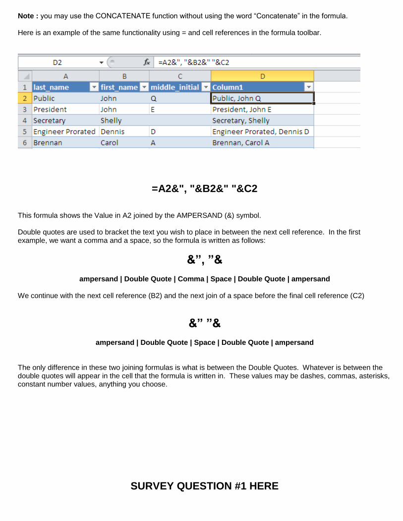
Note : you may use the CONCATENATE function without using the word “Concatenate” in the formula. Here is an example of the same functionality using = and cell references in the formula toolbar.

=A2&", "&B2&" "&C2 This formula shows the Value in A2 joined by the AMPERSAND (&) symbol. Double quotes are used to bracket the text you wish to place in between the next cell reference. In the first example, we want a comma and a space, so the formula is written as follows:

&”, ”&

ampersand | Double Quote | Comma | Space | Double Quote | ampersand We continue with the next cell reference (B2) and the next join of a space before the final cell reference (C2)

&” ”&

ampersand | Double Quote | Space | Double Quote | ampersand The only difference in these two joining formulas is what is between the Double Quotes. Whatever is between the double quotes will appear in the cell that the formula is written in. These values may be dashes, commas, asterisks, constant number values, anything you choose.

SURVEY QUESTION #1 HERE

Concatenating data (joining FIELDS) in MS Query Now that you have learned how to concatenate cells within Excel, let’s take time to explore options on combining and formatting data fields in the query mode. This way, data is returned in the desired format, and columns do not have to be hidden. In the Query mode, with the employee table selected, we click on the first column header in the data preview area and type in the following:

last_name+’, ‘+first_name Just when you thought you were getting the hang of it…. Microsoft changes the game again. In the QUERY MODE, you do not use the ampersand and double quotes, you must use the PLUS (+) sign and a SINGLE quote to bracket the data / field names. Programmers – go figure.

Tab out of the field to view the results.

This is only the beginning….. Combining text fields is one option, you can write rather complex calculations against numeric data from tables. This is not recommended for the faint of heart, as the formula logic in Excel does not always relate to writing a formula in the Query mode. A lot of trial and error will be needed in order to create the desired results. If you are better at writing formulas in Excel, by all means, return the data to Excel, perform the calculations on the spreadsheet and hide unneeded columns. (You may thank me later)

You may run into issues when trying to join fields from multiple tables. You must be sure to define the table name and the field name within the query window. Here is an example of the Job_history table, the jobs table and the cost_codes table. You will notice that the jobs table and the cost_codes table both have the field “description” within their data set.

If I try to perform a shortcut, and type in the desired concatenated field, I receive an error.

Ambiguous column name….. which means the query tool cannot figure out which table to pull the “job_id” and

“description” fields from.

One way to overcome this is to “cheat”. Add the fields to the query manually, then double click on the column heading to see what table.field_name exists. In this example, it shows jobs.description, which means it is the description from the jobs table. If it were the description from the cost_codes table, it would read cost_codes.description.

To concatenate the Job ID and Description, copy the text “jobs.description” from the Field box in the Edit Column

window. Click OK and double click on the job_id column heading and type in the manually entered text separated by the PLUS sign and a SINGLE QUOTE. You should see : job_history.job_id+’ – ‘+

At the end of this text, right click and paste the previously copied text. You should now see: job_history.job_id+' - '+jobs.description

Change the Column heading to JOB, and click OK.

You may now delete the description field from the query, as it was simply used as a reference (or a crutch). With a

bit of practice, you will be able to master manually typing the table and field names within the queries.

Invalid table references : this is what happens when you simply misspell a table or field name. Since there is no field name “job_ids”, you will get the following error :

Ambiguous Reference = field names that exist in multiple tables. Invalid Column Name errors are due to poor

judgement, or poor typing skills.

SURVEY QUESTION #2

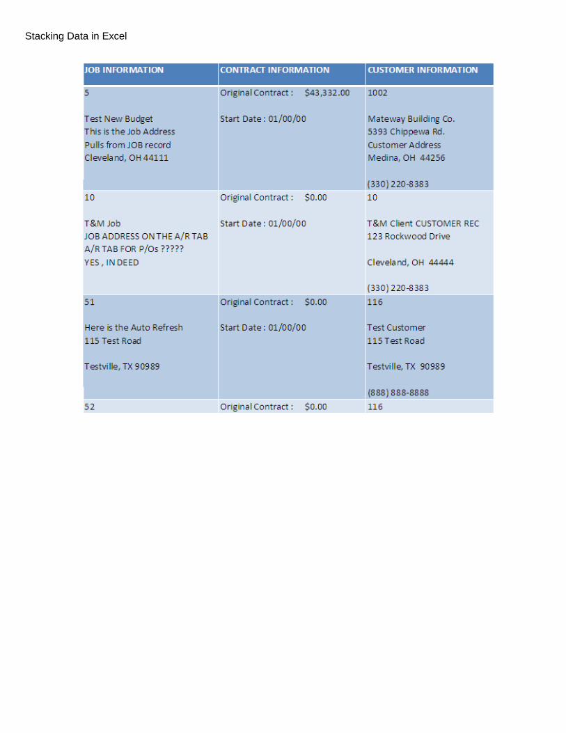
Stacking Data in Excel

When returning data from a query, the table structure limits the data to a very linear format. Using the concatenate function in conjunction with the CHAR(10) formula will allow data to be “stacked” horizontally in a single column. Create a query accessing the customers and jobs table.

Pull in the fields listed below in order: jobs.job_id jobs.description jobs.address_1 jobs.address_2 jobs.city jobs.state jobs.zip_code jobs.original_contract jobs.job_start_date jobs.customer_id costomers.name customers.address_1 customers.address_2 customers.city customers.state customers.zip_code customers.phone_voice

In the Criteria Field, select jobs.job_status and choose Operator – equals / Value A. This will return only active jobs to our spreadsheet.

Decide which data you wish to appear in a single column and insert a column after the last row in that range. In this example, we will put the job number, name and address information all in one cell.

Char(10) is the ASCII code to start a NEW LINE within the cell. In cell H2, enter the following equation:

=A2&CHAR(10)&CHAR(10)&B2

-or-

=concatenate(A2,char(10),char(10),B2) Press enter, or click the check to validate the equation. …not too special, it still looks like a cell that has been concatenated, without spacing to boot.

Right Click on the column heading and select Format Cells:

Click OK with these options selected and resize the column. The data from two individual cells is now “stacked” vertically.

On the Alignment Tab, set the following options: Text Alignment:

Horizontal: Left (Indent) Vertical: Top

Text Control:

Check “Wrap Text”

Continue writing the equation to include all columns A – G. Separate each cell reference with the char(10) code to produce a line feed between the cell references.

=A2&CHAR(10)&CHAR(10)&B2&CHAR(10)&C2&CHAR(10)&D2&CHAR(10)&E2&", "&F2&" "&G2 Pay attention to the change in cells E2, F2 and G2. This is the City, State and Zip Code information. These will not be separated by a line feed. These cells are separated by text designated/defined by the text in between double quotes. Once the formula is written, press enter or validate the formula with the check mark to the left of the formula bar.

Your row height should now be resized to the largest value in a particular column (in this case, the data contained in column H.

Highlight and hide Columns A – G.

Click in the upper-most “cell” on top of the row numbers and to the left of the Column letters to select the entire sheet.

Double click the line that separates the rows. You will know when to double click when the pointer changes to

You have now formatted some of the Job information into a single Column:

Insert a column after the Job Start Date: Here we will “stack” the Original Contract Amount and the Job Start Date…. AND format the cells in the appropriate numeric and date format. Start with some text that will precede the Contract Amount in Column I2.

="Original Contract: "&DOLLAR(I2) The Dollar(cell reference)function will turn the unformatted value into a currency format. Continue the formula to include the CHAR(10) line feed options and include the following to format the Date value in cell J2.

TEXT(J2,"MM/DD/YY") The complete formula is written as follows:

="Original Contract: "&DOLLAR(I2)&CHAR(10)&CHAR(10)&"Start Date: "&TEXT(J2,"MM/DD/YY")

Format Column K in the same manner as Column H by selecting the appropriate settings in the Text Alignment and

Text Control section of the Alignment tab.

What happens when I want to format a phone number within a cell formula:

This is the Formula to be written in Cell S2:

="("&LEFT(R2,3)&") "&MID(R2,4,3)&"-"&RIGHT(R2,4) Looks complicated, but if you break down the individual components between the ampersands (&) – the logic becomes clear: The first part of the equation is the left parenthesis preceding the area code:

=”(“ Then we use the leftmost three digits from cell R2. LEFT(Cell reference, number of characters)

LEFT(R2,3) Complete the Area Code formatting with a right side parenthesis and a space.

“) “ Next, to separate the middle characters in the 4th, 5th and 6th position, use the MID function. MID(cell reference, starting character, number of characters from the starting character)

MID(R2,4,3) Add the Dash between the first three digits “-“ ….And the final 4 characters of the 7 digit phone number. RIGHT(Cell reference, number of characters)

RIGHT(R2,4)

Ultimately we will combine the phone number in a “stacked” column to return all the data for the Customer into a single column:

=L2&CHAR(10)&CHAR(10)&M2&CHAR(10)&N2&CHAR(10)&O2&", "&P2&" "&Q2&CHAR(10)&CHAR(10)&"("&LEFT(R2,3)&") "&MID(R2,4,3)&"-"&RIGHT(R2,4) Hide the columns that are represented in the equation above and you will see the fruits of your labor:

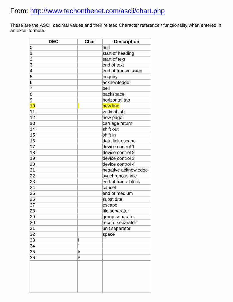
From: http://www.techonthenet.com/ascii/chart.php These are the ASCII decimal values and their related Character reference / functionality when entered in an excel formula.

DEC Char Description

0 null

1 start of heading

2 start of text

3 end of text

4 end of transmission

5 enquiry

6 acknowledge

7 bell

8 backspace

9 horizontal tab

10 new line

11 vertical tab

12 new page

13 carriage return

14 shift out

15 shift in

16 data link escape

17 device control 1

18 device control 2

19 device control 3

20 device control 4

21 negative acknowledge

22 synchronous idle

23 end of trans. block

24 cancel

25 end of medium

26 substitute

27 escape

28 file separator

29 group separator

30 record separator

31 unit separator

32 space

33 !

34 "

35 #

36 $

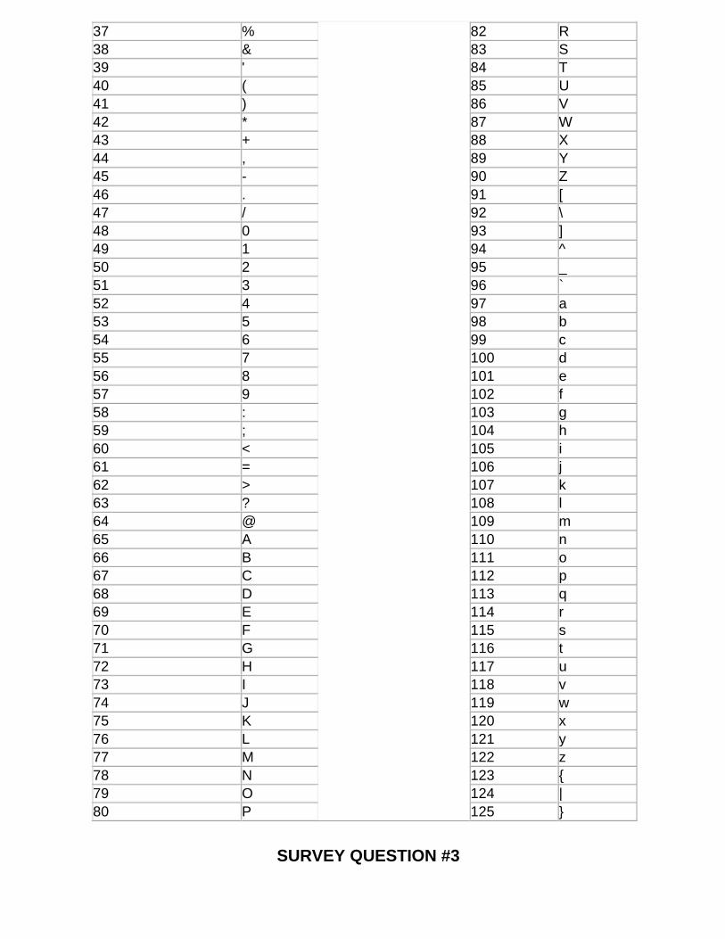
37 % 82 R

38 & 83 S

39 ' 84 T

40 ( 85 U

41 ) 86 V

42 * 87 W

43 + 88 X

44 , 89 Y

45 - 90 Z

46 . 91 [

47 / 92 \

48 0 93 ]

49 1 94 ^

50 2 95 _

51 3 96 `

52 4 97 a

53 5 98 b

54 6 99 c

55 7 100 d

56 8 101 e

57 9 102 f

58 : 103 g

59 ; 104 h

60 < 105 i

61 = 106 j

62 > 107 k

63 ? 108 l

64 @ 109 m

65 A 110 n

66 B 111 o

67 C 112 p

68 D 113 q

69 E 114 r

70 F 115 s

71 G 116 t

72 H 117 u

73 I 118 v

74 J 119 w

75 K 120 x

76 L 121 y

77 M 122 z

78 N 123 {

79 O 124 |

80 P 125 }

SURVEY QUESTION #3