Confidence Bands for the Logistic and

Probit Regression Models Over Intervals

Lucy Kerns

Department of Mathematics and Statistics

Youngstown State University

Youngstown OH 44555

xlu@ysu.edu

Summary

This article presents methods for the construction of two-sided and one-sided simulta-

neous hyperbolic bands for the logistic and probit regression models when the predictor

variable is restricted to a given interval. The bands are constructed based on the asymp-

totic properties of the maximum likelihood estimators. Past articles have considered

building two-sided asymptotic confidence bands for the logistic model, such as Piegorsch

and Casella (1988). However, the confidence bands given by Piegorsch and Casella are

conservative under a single interval restriction, and it is shown in this article that their

bands can be sharpened using the methods proposed here. Furthermore, no method has

yet appeared in the literature for constructing one-sided confidence bands for the logistic

model, and no work has been done for building confidence bands for the probit model, over

a limited range of the predictor variable. This article provides methods for computing

critical points in these areas.

Keywords: One-sided confidence bands; Two-sided confidence bands; Logistic regression;

Probit regression; Simple linear regression

1

arX

iv:1

604.

0124

2v1

[m

ath.

ST]

5 A

pr 2

016

1 Introduction

Logistic and probit regression models are widely used for modeling dichotomous outcomes,

and have been increasingly applied in medical research, public health research, environ-

mental science, and many other fields, such as human behavior modeling (Chou, Lu, and

Mao, 2002), environmental modeling (Pradhan and Lee, 2010), and biomedical research

(Austin and Steyerberg, 2014). The logistic and probit regression models are statistical

methods that allow one to estimate the response probability for a dichotomous response,

that is, a response which is binary, taking values 1 (success, normal, positive, etc.) and 0

(failure, abnormal, negative, etc.). In this article, we consider the case where the binary

response variable Y is determined by a predictor variable x, and the response probability

is:

P (Y = 1) = p(x) =

1/[1 + exp(−c′β)], logistic model

Φ(c′β), probit model

where c = (1 x)′, β = (β0 β1)′, and Φ is the cumulative distribution function (cdf) of

the standard normal distribution.

The construction of confidence bands on p(x) is often of interest, and we will use the

following link functions to transform the problem of constructing confidence bands for the

response probability p(x) to the problem of constructing confidence bands for the linear

predictor c′β on which the bands are defined.

logit(p(x)) = loge

[p(x)

1− p(x)

]= c′β, logistic regression

probit(p(x)) = Φ−1(p(x)) = c′β, probit regression

There is a wealth of literature on building exact or conservative two-sided bands for

the linear predictor c′β with one or more than one predictor variable. This includes the

work of Scheffe (1953), and Working & Hotelling (1929), among others. Many authors

have improved earlier work by restricting the predictor variables to given intervals, in-

cluding Wynn and Bloomfield (1971), Casella and Strawderman (1980), and Uusipaikka

(1983). Liu et al. (2005) developed a simulation-based method for constructing two-sided

confidence bands over a restricted region for the multiple regression model. Less work has

1

been done on the construction of one-sided (lower or upper) confidence bands for linear

regression. With no restriction on the predictor variable, Hochberg and Quade (1975)

developed a method for constructing one-sided bands in the multiple regression setting.

When the predictor variable is constrained to a pre-specified interval, Bohrer and Francis

(1972) gave exact one-sided hyperbolic confidence bands for the simple linear case. Pan

et al. (2003) extended Uusipaikka’s work (1983) to the computation of one-sided bands

under a single interval restriction. Liu et al.’s article (2008) summarized several existing

methods and also provided new methods for the construction of two-sided and one-sided

confidence bands with a restricted predictor variable.

Much less work has been done on constructing confidence bands for the logistic re-

gression model. Brand, Pinnock, and Jackson (1973) constructed confidence bands for

both p(x) and the inverse of p(x) when there is one predictor variable and no constraints

exist on the predictor variable. Hauck (1983) extended their work to more than one pre-

dictor variable yet still with no constraints. In the case of restricted predictor variables,

Piegorsch and Casella (1988) extended the work of Casella and Strawderman (1980) from

the multiple regression model to the logistic case. The method of Casella and Straw-

derman produced asymptotic two-sided bands over a particular constrained region of

predictor variables. However, if the restricted region on predictor variables is rectangular,

the resulting confidence bands are rather conservative even with large samples.

Wei Liu’s book (2010, Chapter 8) presented confidence bands for the logistic model

with more than one explanatory variable. The method utilized simulation-based confi-

dence bands (Liu et al. (2005)) for the linear predictor c′β in the multiple linear model,

and the desired bands for the logistic model were then obtained via the logit link function.

The new contribution of this paper is that we provide explicit expressions for determining

the critical values in the logistic setting. Wei Liu’s method is very broad, but relies on

simulation. Our method is more focused but admits tractable forms.

Furthermore, no work has yet appeared for building one-sided confidence bands for the

logistic regression model when the predictor variable is bounded on a given interval, and no

methods have been developed for constructing both two-sided and one-sided bands for the

probit regression model with a restricted predictor variable. In this paper, we center our

2

attention on building asymptotic two-sided and one-sided hyberbolic confidence bands for

the logistic and probit models over a limited range of the predictor variable, say, between

(a, b), where a and b are constants.

For the logistic and probit models, we denote the ML estimator of β by β, and under

certain regularity conditions (Kendall and Stuart (1979)), β follows asymptotically as:

β ∼ ASN2(β,F−1),

where F is the Fisher information matrix. It is well known that the logistic model has an

explicit formula for the Fisher information matrix, while the probit model does not, but

the information matrix can be obtained through numerical methods.

For x ∈ (a, b), where a and b are given constants, a 100(1− α)% two-sided hyperbolic

band for the linear function c′β has the form

c′β ∈ c′β ± w(c′F−1c)1/2,

where c = (1 x)′ and w satisfies

P [c′β ∈ c′β ± w(c′F−1c)1/2, for all x ∈ (a, b)] = 1− α. (1)

An upper 100(1− α)% one-sided hyperbolic band for the linear function c′β has the

form

c′β ≤ c′β + wu(c′F−1c)1/2,

where wu satisfies

P [c′β ≤ c′β + wu(c′F−1c)1/2, for all x ∈ (a, b)] = 1− α. (2)

A 100(1− α)% lower one-sided hyperbolic band for c′β can be defined similarly.

Since both logit and probit functions are monotonically increasing functions, 100(1−

α)% two-sided confidence bands for p(x) in the logistic regression model are given by

1 + exp[−c′β + w(c′F−1c)1/2]−1 ≤ p(x) ≤ 1 + exp[−c′β − w(c′F−1c)1/2]−1,

and 100(1 − α)% two-sided confidence bands for p(x) in the probit regression model are

given by

Φ(c′β − w(c′F−1c)1/2) ≤ p(x) ≤ Φ(c′β + w(c′F−1c)1/2).

3

Similarly, 100(1− α)% upper confidence bands for p(x) are given by

p(x) ≤

1 + exp[−c′β − wu(c′F−1c)1/2]−1, logistic model

Φ(c′β + wu(c′F−1c)1/2), probit model

In what follows, we consider the logistic model and focus on Equations (1) and (2).

In particular, we propose methods to find the critical values w in Equation (1) for the

two-sided case and wu in Equation (2) for the one-sided case under the logistic model.

The derivation of the critical values under the probit model is the same except F−1 is

replaced by Ω−1.

Both the logistic and probit models are special cases of the generalized linear model

(GLM), and the methodology proposed here can also be applied to other forms of GLM

(the complementary-log-log model, for example), that can be transformed into the stan-

dard regression model via a link function. In each case, a set of simulations are required

to confirm the validity of the method in small samples, thus in the interest of brevity only

logistic and probit models are considered here. We devote most of our attention to the

logistic model to illustrate the methodology.

Liu et al.’s article (2008) presents several methods for the construction of two-sided

and one-sided confidence bands for the simple linear model with a restricted predictor

variable. Since we can transform the logistic and probit regression setting to the simple

linear regression setting via the link functions (logit and probit), we extend their work

to the logistic and probit regression models and develop methods to derive asymptotic

confidence bands for large samples. This paper is organized as follows. We give the

general setting of the problem in Section 1. Two-sided confidence bands are discussed in

Section 2, and Section 3 presents the results in the one-sided case. In Section 4, a Monte

Carlo simulation is run to investigate how well the asymptotic approximation holds for

small sample sizes. An example is given in Section 5 to illustrate the proposed methods.

4

2 Two-Sided Bands

Our construction of confidence bands are based on the methods given by Liu et al. (2008).

There are undoubtedly some similarities between the methods presented here and in their

review. The main difference between their method and ours lies at the beginning of

the derivation. The formulation in their review relied on a standard bivariate t random

variable (See Equations (13) and (14) in their review), while the derivation given here

involves a standard z bivariate random variable, as will be soon shown. As a result of

this reformulation, our critical values are based on a chi-square random variable, instead

of an F variate. In the interest of completeness, we include most of the computational

details regarding the critical values w and wu.

The Fisher information matrix F−1 is a positive semi-definite symmetric matrix, so

there exists a positive semi-definite matrix B such that F−1 = B2. Then

z = B−1(β − β) ∼ N2(0, I).

Define the polar coordinates of z = (z1, z2)′, (Rz, Qz), by

z1 = Rz cosQz, z2 = Rz sinQz, for Rz ≥ 0 and Qz ∈ [0, 2π].

It is well known that R2z has the χ2

2 distribution and is statistically independent of Qz,

which has a uniform [0, 2π] distribution. Write Equation (1) as

P [c′β ∈ c′β ± w(c′F−1c)1/2, for all x ∈ (a, b)]

= P

[supx∈(a,b)

|c′β − c′β|(c′F−1c)1/2

< w

]

= P

[supx∈(a,b)

|(Bc)′z|‖Bc‖

< w

](3)

Notice that for a given vector u ∈ R2 and a number w > 0, z : u′z/‖u‖ = w represents

a straight line that is perpendicular to the vector u and is on the same side of the origin

as the vector u. The perpendicular distance from the origin to this line is w. Therefore,

the set defined by

z : |u′z|/‖u‖ < w ⊂ R2

5

consists of all points that are sandwiched between two parallel straight lines u′z/‖u‖ = w

and u′z/‖u‖ = −w. Therefore, letting Bc = u, Equation (3) can be further expressed

as:

P

[supx∈(a,b)

|(u)′z|‖u‖

< w

]= Pz ∈ R2, (4)

where R2 = ∩x∈(a,b)R2(x), and R2(x) = z : |u′z|/‖u‖ < w. R2 is depicted in Fig-

ure 1(a). We can rotate the region R2 around the origin so that the angle φ between the

two vectors ua = B(1 a) and ub = B(1 b) is equally divided by the z1-axis. The new

region, denoted by R∗2, is depicted in Figure 1(b). Because of the rotation invariance of

the normal distribution, we have Pz ∈ R2 = Pz ∈ R∗2, and R∗2 can be expressed as

R∗2 = z : |u′z|/‖u‖ < w, for all u ∈ E(φ),

where E(φ) is a cone depicted as the shaded area in Figure 1(b), and E(φ) = u : u2 >

‖u‖cos(φ/2). Therefore, the simultaneous confidence level is equal to

P

[sup

u∈E(φ)

|u′z|‖u‖

< w

]= Pz ∈ R∗2. (5)

(a) Region R2 (b) Region R∗2

Figure 1: The Regions R2 and R∗2

6

2.1 Method 1: Finding Expression for the Supremum

This method is based on finding an exact expression for the supremum. Notice that

|u′z|‖u‖

= ‖z‖ |u′z|

‖u‖‖z‖= ‖z‖|cos(θuz)|,

where θuz is the angle between u and z. Denote Ψ1 = [−φ/2, φ/2] ∪ [π − φ/2, π + φ/2],

Ψ2 = [φ/2, π/2]∪ [π+ φ/2, 3π/2], and Ψ3 = [π/2, π− φ/2]∪ [3π/2,−φ/2]. Since cos(θ) is

monotonically decreasing on [0, π], we have the following results:

supu∈E(φ)

|cos(θuz)| =

1 if θz ∈ Ψ1,

|cos(θz − φ/2)| if θz ∈ Ψ2,

|cos(θz + φ/2)| if θz ∈ Ψ3.

Hence, the probability on the left side of Equation (5) can be written as

Pθz ∈ Ψ1, ‖z‖ < w+ Pθz ∈ Ψ2, ‖z‖|cos(θz − φ/2)| < w

+ Pθz ∈ Ψ3, ‖z‖|cos(θz + φ/2)| < w

=φ

πP‖z‖ < w

+ 2

∫ π/2

φ/2

1

2πP‖z‖|cos(θ − φ/2)| < w dθ

+ 2

∫ π−φ/2

π/2

1

2πP‖z‖|cos(θ + φ/2)| < w dθ

=φ

πPRz < w

+2

π

∫ π/2

φ/2

PRz|cos(θ − φ/2)| < w dθ

=φ

πχ22(w

2) +2

π

∫ π/2

φ/2

χ22

(w2

cos2(θ − φ/2)

)dθ, (6)

where χ22(.) is the cdf of a chi-squared distribution with 2 degrees of freedom.

2.2 Method 2: A Method Based on Wynn & Bloomfield’s Ap-

proach

This method calculates Pz ∈ R∗2 directly, and is based on the method given by Wynn

& Bloomfield (1971). It can be seen from Figure 1(b) that the region R∗2 is made up of

7

the circle with radius w and the remaining area. The probability that z lies in the circle

is given by

P‖z‖ < w = PRz < w = χ22(w

2) (7)

The probability that z lies in the remaining region is 4 times the probability that z lies

in the slanted-line shaded area in Figure 1(b), which is

4Pθz ∈ [φ/2, π/2], ‖z‖ > w, ‖z‖cos[θz − φ/2] < w

= 4Pθz ∈ [φ/2, π/2], w < ‖z‖ < w/cos[θz − φ/2]

= 4

∫ π/2

φ/2

1

2πPw < ‖z‖ < w/cos[θ − φ/2] dθ

=2

π

∫ π/2

φ/2

[χ22

(w2

cos2[θ − φ/2]

)− χ2

2(w2)

]dθ (8)

Combining Equation (7) and Equation (8), we have the following:

Pz ∈ R∗2 =φ

πχ22(w

2) +2

π

∫ π/2

φ/2

[χ22

(w2

cos2[θ − φ/2]

)]dθ, (9)

which is equal to Equation (6).

3 One-Sided Bands

Similar to the two-sided case, we can express Equation (2) as

P [c′β ≤ c′β + wu(c′F−1c)1/2, for all x ∈ (a, b)]

= P

[supx∈(a,b)

(Bc)′z

‖Bc‖< wu

]= Pz ∈ R1, (10)

where R1 ⊂ R2 is given by R1 = ∩x∈(a,b)R1(x), and R1(x) = z : u′z/‖u‖ < w with

u = Bc. Rotating the region R1 around the origin the same way as we did in the two-

sided case, we obtain a new region R∗1 with the property Pz ∈ R1 = Pz ∈ R∗1. The

new region is depicted in Figure 2, and has the expression

R∗1 = z : u′z/‖u‖ < w, for all u ∈ E(φ),

8

where E(φ) is defined the same as before. Therefore, the simultaneous confidence level is

equal to

P

[sup

u∈E(φ)

u′z

‖u‖< wu

]= Pz ∈ R∗1. (11)

Figure 2: Region R∗1

3.1 Method 1: Finding Expression for the Supremum

Similar to the two-sided bands, this method is based on finding the supremum in Equa-

tion (11). As before, we writeu′z

‖u‖= ‖z‖cos(θuz),

where θuz is the angle between u and z. Denote Ψ1 = [−φ/2, φ/2], Ψ2 = [φ,−π/2], and

Ψ3 = [φ/2, π]. Because of the monotonicity of cos(θ) on [0, π], we have

supu∈E(φ)

cos(θuz) =

1 if θz ∈ Ψ1,

cos[θz + φ/2] if θz ∈ Ψ2,

cos[θz − φ/2] if θz ∈ Ψ3.

9

Hence, the probability on the left side of Equation (11) can be written as

Pθz ∈ Ψ1, ‖z‖ < wu+ Pθz ∈ Ψ2, ‖z‖cos[θz + φ/2] < wu

+ Pθz ∈ Ψ3, ‖z‖cos[θz − φ/2] < wu

=φ

2πP‖z‖ < wu

+ 2

∫ π

φ/2

1

2πP‖z‖cos[θ − φ/2] < wu dθ

=φ

2πP‖z‖ < wu

+ 2

∫ (π+φ)/2

φ/2

1

2πP‖z‖cos[θ − φ/2] < wu dθ

+ 2

∫ π

(π+φ)/2

1

2πP‖z‖cos[θ − φ/2] < wu dθ

=φ

2πχ22(w

2u) +

π − φ2π

+1

π

∫ π/2

0

P‖z‖ < wucos(θ)

dθ. (12)

The last step follows from the fact that supremum of cos(θuz) is negative when θz ∈

[π, (3π − φ)/2] ∪ [(π + φ)/2, π].

3.2 Method 2: A Method Based on Bohrer & Francis’s Ap-

proach

This method is similar to that for the two-sided case in Section 2.2, and is based on the

method given by Bohrer & Francis (1972). Notice that the region R∗1 can be partitioned

into four sub-regions, C1, C2, C3, and C4. The probability Pz ∈ R∗1 can be calculated

by summing up the probabilities that z lies in the four sub-regions. The probability that

z falls in C1 is equal to

Pz ∈ C1 = Pθz ∈ [(π − φ)/2, (π + φ)/2], ‖z‖ < wu

=φ

2πP‖z‖ < wu

=φ

2πχ22(w

2u). (13)

The probability that z falls into the region C2 is given by

Pz ∈ C2 = Pθz ∈ [(π + φ)/2, (3π − φ)/2] =π − φ

2π. (14)

10

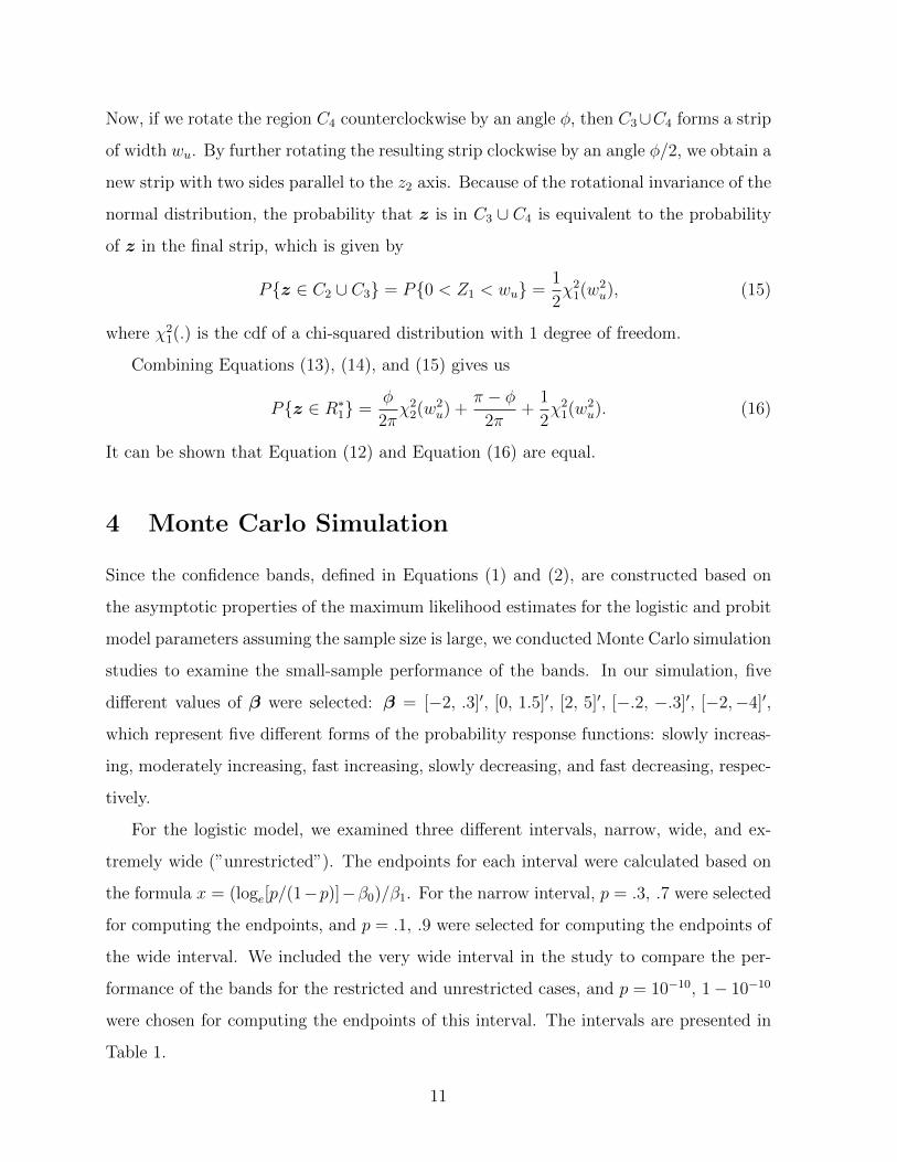
Now, if we rotate the region C4 counterclockwise by an angle φ, then C3∪C4 forms a strip

of width wu. By further rotating the resulting strip clockwise by an angle φ/2, we obtain a

new strip with two sides parallel to the z2 axis. Because of the rotational invariance of the

normal distribution, the probability that z is in C3 ∪ C4 is equivalent to the probability

of z in the final strip, which is given by

Pz ∈ C2 ∪ C3 = P0 < Z1 < wu =1

2χ21(w

2u), (15)

where χ21(.) is the cdf of a chi-squared distribution with 1 degree of freedom.

Combining Equations (13), (14), and (15) gives us

Pz ∈ R∗1 =φ

2πχ22(w

2u) +

π − φ2π

+1

2χ21(w

2u). (16)

It can be shown that Equation (12) and Equation (16) are equal.

4 Monte Carlo Simulation

Since the confidence bands, defined in Equations (1) and (2), are constructed based on

the asymptotic properties of the maximum likelihood estimates for the logistic and probit

model parameters assuming the sample size is large, we conducted Monte Carlo simulation

studies to examine the small-sample performance of the bands. In our simulation, five

different values of β were selected: β = [−2, .3]′, [0, 1.5]′, [2, 5]′, [−.2, −.3]′, [−2,−4]′,

which represent five different forms of the probability response functions: slowly increas-

ing, moderately increasing, fast increasing, slowly decreasing, and fast decreasing, respec-

tively.

For the logistic model, we examined three different intervals, narrow, wide, and ex-

tremely wide (”unrestricted”). The endpoints for each interval were calculated based on

the formula x = (loge[p/(1−p)]−β0)/β1. For the narrow interval, p = .3, .7 were selected

for computing the endpoints, and p = .1, .9 were selected for computing the endpoints of

the wide interval. We included the very wide interval in the study to compare the per-

formance of the bands for the restricted and unrestricted cases, and p = 10−10, 1− 10−10

were chosen for computing the endpoints of this interval. The intervals are presented in

Table 1.

11

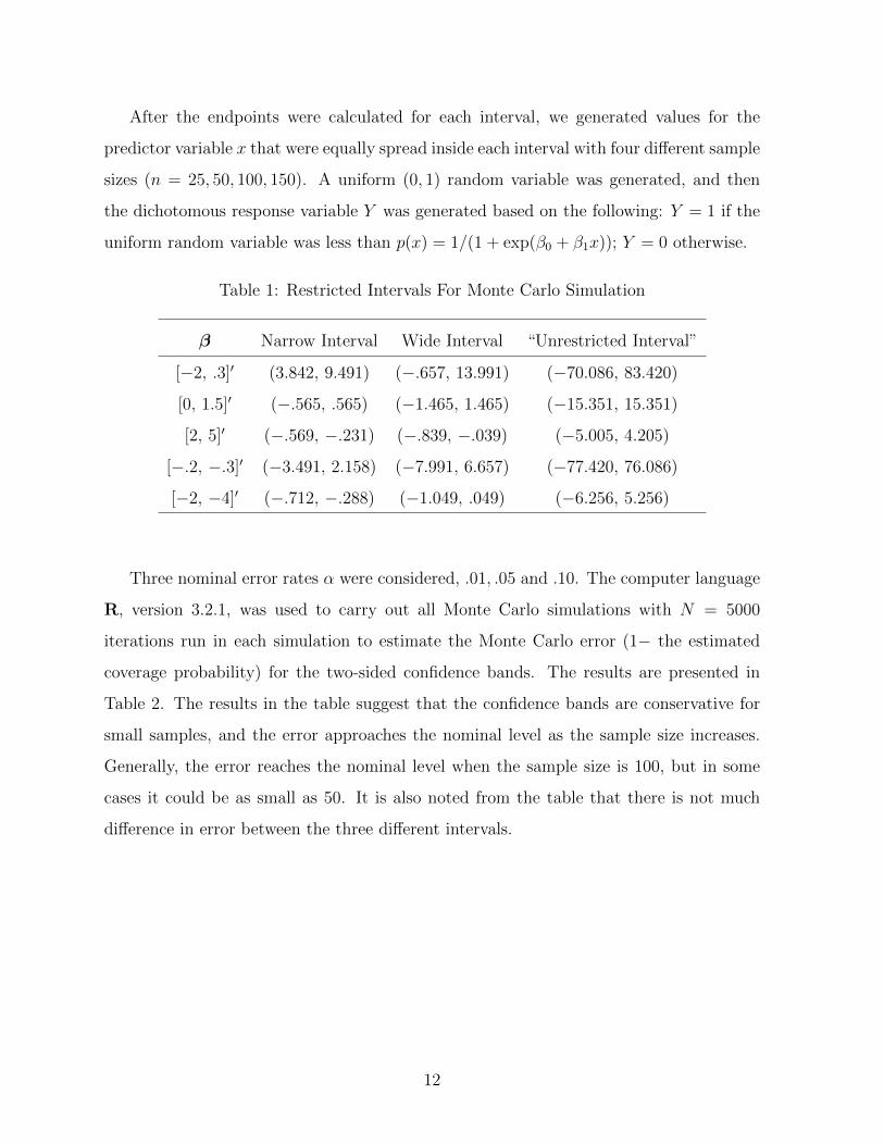
After the endpoints were calculated for each interval, we generated values for the

predictor variable x that were equally spread inside each interval with four different sample

sizes (n = 25, 50, 100, 150). A uniform (0, 1) random variable was generated, and then

the dichotomous response variable Y was generated based on the following: Y = 1 if the

uniform random variable was less than p(x) = 1/(1 + exp(β0 + β1x)); Y = 0 otherwise.

Table 1: Restricted Intervals For Monte Carlo Simulation

β Narrow Interval Wide Interval “Unrestricted Interval”

[−2, .3]′ (3.842, 9.491) (−.657, 13.991) (−70.086, 83.420)

[0, 1.5]′ (−.565, .565) (−1.465, 1.465) (−15.351, 15.351)

[2, 5]′ (−.569, −.231) (−.839, −.039) (−5.005, 4.205)

[−.2, −.3]′ (−3.491, 2.158) (−7.991, 6.657) (−77.420, 76.086)

[−2, −4]′ (−.712, −.288) (−1.049, .049) (−6.256, 5.256)

Three nominal error rates α were considered, .01, .05 and .10. The computer language

R, version 3.2.1, was used to carry out all Monte Carlo simulations with N = 5000

iterations run in each simulation to estimate the Monte Carlo error (1− the estimated

coverage probability) for the two-sided confidence bands. The results are presented in

Table 2. The results in the table suggest that the confidence bands are conservative for

small samples, and the error approaches the nominal level as the sample size increases.

Generally, the error reaches the nominal level when the sample size is 100, but in some

cases it could be as small as 50. It is also noted from the table that there is not much

difference in error between the three different intervals.

12

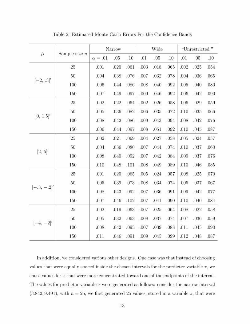
Table 2: Estimated Monte Carlo Errors For the Confidence Bands

β Sample size nNarrow Wide “Unrestricted ”

α = .01 .05 .10 .01 .05 .10 .01 .05 .10

[−2, .3]′

25 .001 .020 .061 .003 .018 .065 .002 .025 .054

50 .004 .038 .076 .007 .032 .078 .004 .036 .065

100 .006 .044 .086 .008 .040 .092 .005 .040 .080

150 .007 .049 .097 .009 .046 .092 .006 .042 .090

[0, 1.5]′

25 .002 .022 .064 .002 .026 .058 .006 .029 .059

50 .005 .036 .082 .006 .035 .072 .010 .035 .066

100 .008 .042 .086 .009 .043 .094 .008 .042 .076

150 .006 .044 .097 .008 .051 .092 .010 .045 .087

[2, 5]′

25 .002 .021 .069 .004 .027 .058 .005 .024 .057

50 .004 .036 .080 .007 .044 .074 .010 .037 .060

100 .008 .040 .092 .007 .042 .084 .009 .037 .076

150 .010 .048 .101 .008 .049 .089 .010 .046 .085

[−.3, −.2]′

25 .001 .020 .065 .005 .024 .057 .008 .025 .070

50 .005 .039 .073 .008 .034 .074 .005 .037 .067

100 .008 .043 .092 .007 .036 .091 .009 .042 .077

150 .007 .046 .102 .007 .041 .090 .010 .040 .084

[−4, −2]′

25 .002 .019 .063 .007 .025 .064 .008 .022 .058

50 .005 .032 .063 .008 .037 .074 .007 .036 .059

100 .008 .042 .095 .007 .039 .088 .011 .045 .090

150 .011 .046 .091 .009 .045 .099 .012 .048 .087

In addition, we considered various other designs. One case was that instead of choosing

values that were equally spaced inside the chosen intervals for the predictor variable x, we

chose values for x that were more concentrated toward one of the endpoints of the interval.

The values for predictor variable x were generated as follows: consider the narrow interval

(3.842, 9.491), with n = 25, we first generated 25 values, stored in a variable z, that were

13

equally spaced in (0, 1). Then we used the transformation y = z6 to make the values of y

concentrate toward the lower end of the interval, 0. Finally, we let x = 5.649y + 3.842 to

obtain the desired x values which fell inside the chosen interval and were clustered at the

lower end, 3.842.

The other case examined was when most of the x values were located at the center of

the chosen intervals, which were generated as follows: for the narrow interval (3.842, 9.491)

centered at 6.6665, with n = 25, we first generated 25 values that were equally spaced in

(−1, 1), which were stored in a variable called z. Then we used the transformation y = z5

to make the values of y concentrate toward the center of the interval (−1, 1), which is 0.

Finally, we let x = 5.649/2 ∗ y + 6.6665 to obtain the desired x values which fell inside

the chosen interval and were concentrated at the center of the interval.

Since the estimated error rates presented in Table 2 are similar at three different α

values, we chose to perform Monte Carlo simulations at α = .05 for these two additional

cases. The results are given in Table 3, and it is clear that the results are consistent with

what we observed from Table 2. We also ran Monte Carlo simulations for the one-sided

bands in the logistic model, and for both bands in the probit model, and again, the results

agree with the two-sided case for the logistic model; those results are not presented here

to avoid driving the size of the paper to cumbersome levels.

14

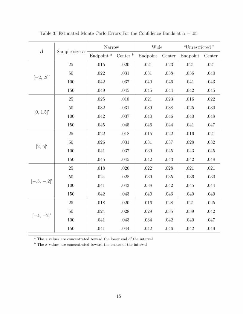
Table 3: Estimated Monte Carlo Errors For the Confidence Bands at α = .05

β Sample size nNarrow Wide “Unrestricted ”

Endpoint a Center b Endpoint Center Endpoint Center

[−2, .3]′

25 .015 .020 .021 .023 .021 .021

50 .022 .031 .031 .038 .036 .040

100 .042 .037 .040 .046 .041 .043

150 .049 .045 .045 .044 .042 .045

[0, 1.5]′

25 .025 .018 .021 .023 .016 .022

50 .032 .031 .039 .038 .025 .030

100 .042 .037 .040 .046 .040 .048

150 .045 .045 .046 .044 .041 .047

[2, 5]′

25 .022 .018 .015 .022 .016 .021

50 .026 .031 .031 .037 .028 .032

100 .041 .037 .039 .045 .043 .045

150 .045 .045 .042 .043 .042 .048

[−.3, −.2]′

25 .018 .020 .022 .028 .021 .021

50 .024 .028 .039 .035 .036 .030

100 .041 .043 .038 .042 .045 .044

150 .042 .043 .040 .046 .040 .049

[−4, −2]′

25 .018 .020 .016 .028 .021 .025

50 .024 .028 .029 .035 .039 .042

100 .041 .043 .034 .042 .040 .047

150 .041 .044 .042 .046 .042 .049

a The x values are concentrated toward the lower end of the intervalb The x values are concentrated toward the center of the interval

15

5 Example

If we restrict the independent variable to an interval, the resulting confidence bands will

be narrower than the unconstrained bands. Here, we use the data provided by LaVelle

(1986) to illustrate the proposed method. The data are presented in Table 4, and these

were the same data that were considered by Piegorsch and Casella (1988). The study in

LaValle (1986) investigated the comutagenic effects of chromate on frameshift mutagenesis

in bacterial assays. The results presented here are findings for the bacterium E. coli, strain

343/435. A control and five doses of the suspected mutagen, 9-Aminoacridine (9-AA) are

reported in Table 4.

Table 4: Mutagenicity of 9-Aminoacridine in E. coli strains 343/435

Dose -∗ .8 2.4 8.0 24 80

Log-dose -1.374 -.223 0.875 2.079 3.178 4.382

Response 7/96 28/96 64/96 54/96 81/96 96/96∗The first data pair corresponds to a zero-dose control. The log-dose

for this datum was calculated using consecutive-dose average spacing

(Margolin et al., 1986).

As pointed out by Piegorsch and Casella, rather than report confidence bands over the

whole real line, it is often of interest to report narrower bands over constrained intervals.

Furthermore, it is often noted that human exposure to environmental toxins usually occurs

at low dose levels. Restricting dose levels enables us to direct our attention to intervals

toward the lower end, and hence improve the confidence limits greatly.

We fit a logistic model to the data using the log-dose level as our predictor variable x,

and the ML estimators from the logistic fit are β0 = −.789, and β1 = .854. The inverse of

the Fisher information matrix is F−1 =

0.017 −0.005

−0.005 0.005

. If we restrict the predictor

variable to an interval (−1.3, .8), then ua = (0.163 − 0.109) , ub = (0.106 0.0234),

and the angle between these two vectors are φ = 0.809. The two methods for two-sided

bands give the same value for the critical point, w = 2.206, at a 95% confidence level.

16

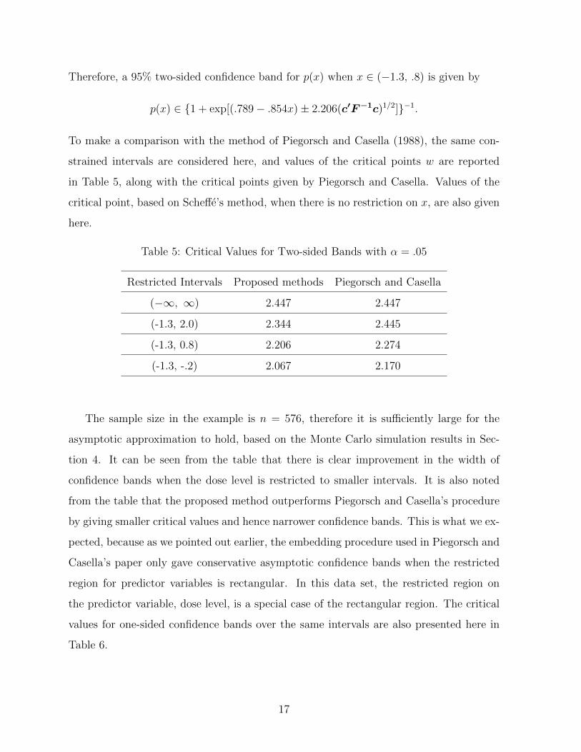
Therefore, a 95% two-sided confidence band for p(x) when x ∈ (−1.3, .8) is given by

p(x) ∈ 1 + exp[(.789− .854x)± 2.206(c′F−1c)1/2]−1.

To make a comparison with the method of Piegorsch and Casella (1988), the same con-

strained intervals are considered here, and values of the critical points w are reported

in Table 5, along with the critical points given by Piegorsch and Casella. Values of the

critical point, based on Scheffe’s method, when there is no restriction on x, are also given

here.

Table 5: Critical Values for Two-sided Bands with α = .05

Restricted Intervals Proposed methods Piegorsch and Casella

(−∞, ∞) 2.447 2.447

(-1.3, 2.0) 2.344 2.445

(-1.3, 0.8) 2.206 2.274

(-1.3, -.2) 2.067 2.170

The sample size in the example is n = 576, therefore it is sufficiently large for the

asymptotic approximation to hold, based on the Monte Carlo simulation results in Sec-

tion 4. It can be seen from the table that there is clear improvement in the width of

confidence bands when the dose level is restricted to smaller intervals. It is also noted

from the table that the proposed method outperforms Piegorsch and Casella’s procedure

by giving smaller critical values and hence narrower confidence bands. This is what we ex-

pected, because as we pointed out earlier, the embedding procedure used in Piegorsch and

Casella’s paper only gave conservative asymptotic confidence bands when the restricted

region for predictor variables is rectangular. In this data set, the restricted region on

the predictor variable, dose level, is a special case of the rectangular region. The critical

values for one-sided confidence bands over the same intervals are also presented here in

Table 6.

17

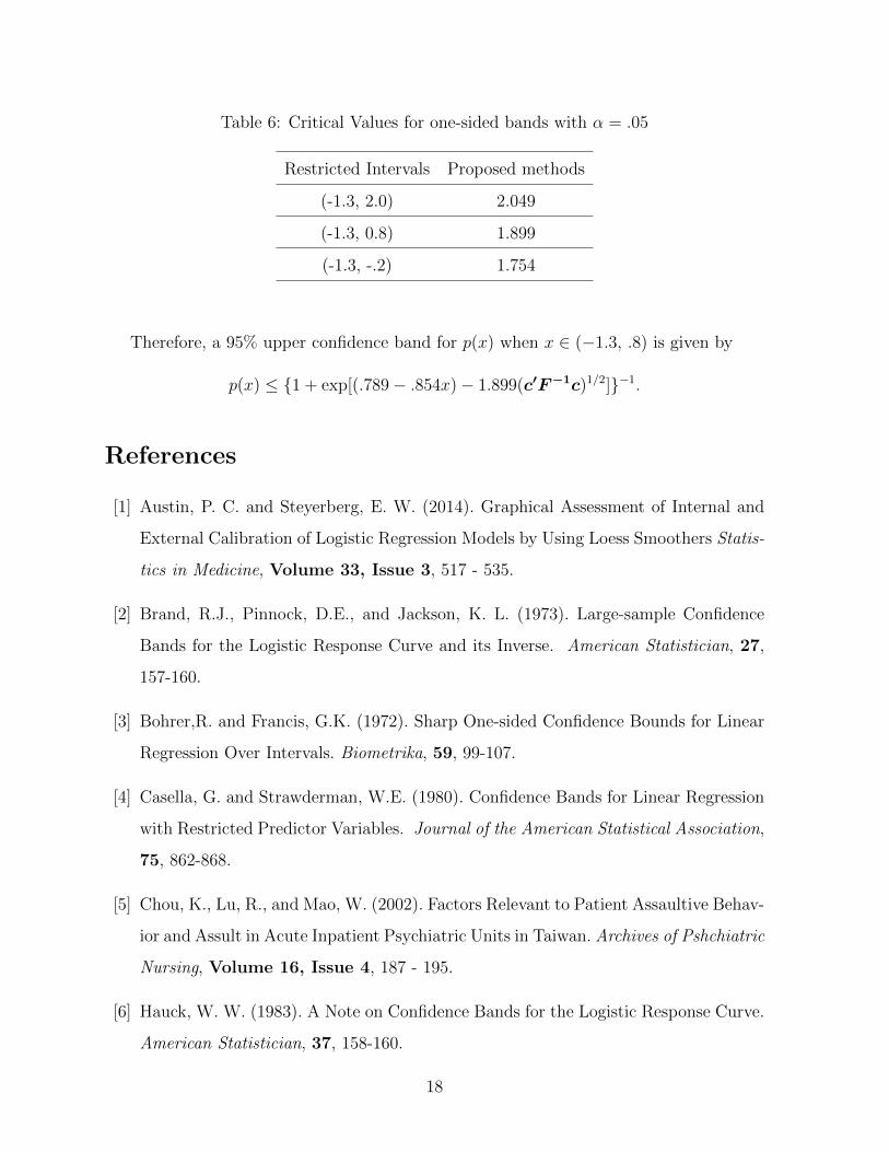
Table 6: Critical Values for one-sided bands with α = .05

Restricted Intervals Proposed methods

(-1.3, 2.0) 2.049

(-1.3, 0.8) 1.899

(-1.3, -.2) 1.754

Therefore, a 95% upper confidence band for p(x) when x ∈ (−1.3, .8) is given by

p(x) ≤ 1 + exp[(.789− .854x)− 1.899(c′F−1c)1/2]−1.

References

[1] Austin, P. C. and Steyerberg, E. W. (2014). Graphical Assessment of Internal and

External Calibration of Logistic Regression Models by Using Loess Smoothers Statis-

tics in Medicine, Volume 33, Issue 3, 517 - 535.

[2] Brand, R.J., Pinnock, D.E., and Jackson, K. L. (1973). Large-sample Confidence

Bands for the Logistic Response Curve and its Inverse. American Statistician, 27,

157-160.

[3] Bohrer,R. and Francis, G.K. (1972). Sharp One-sided Confidence Bounds for Linear

Regression Over Intervals. Biometrika, 59, 99-107.

[4] Casella, G. and Strawderman, W.E. (1980). Confidence Bands for Linear Regression

with Restricted Predictor Variables. Journal of the American Statistical Association,

75, 862-868.

[5] Chou, K., Lu, R., and Mao, W. (2002). Factors Relevant to Patient Assaultive Behav-

ior and Assult in Acute Inpatient Psychiatric Units in Taiwan. Archives of Pshchiatric

Nursing, Volume 16, Issue 4, 187 - 195.

[6] Hauck, W. W. (1983). A Note on Confidence Bands for the Logistic Response Curve.

American Statistician, 37, 158-160.

18

[7] LaVelle, J. M. (1986). Potassium Chromate Potentiates Frameshift Mutagenesis in

E. coli. and S. typhimurium. Mutation Research, 171, 1-10.

[8] Margolin, B.H., Resnick, M.A., Rimpo, J.Y., Archer, P., Galloway, S.M., Bloom,

A.D., and Zeiger, E. (1986). Statistical Analysis for in Vitro. Cytogenic Assays Using

Chinese Hamster Ovary Cells. Enviromental Mutagenesis, 8, 183-204.

[9] Hochberg, Y. and Quade, D. (1975). One-sided Simultaneous Confidence Bands on

Regression Surfaces with Intercepts. Journal of the American Statistical Association,

70, 889-891.

[10] Kendall, M. and Stuart, A. (1979). The Advanced Theory of Statistics, Volume II:

Inference and Relationship,. New York: Macmillan.

[11] Pradhan, B. and Lee, S. (2010). Delineation of Landslide Hazard Areas on Penang Is-

land, Malaysia, By Using Frequency Ratio, Logistic Regression, and Artificial Neural

Network Models. Environmental Earth Science, 60, 1037-1054.

[12] Piegorsch, W.W. and Casella, G. (1988). Confidence Bands for Logisic Regression

with Restricted Predictor Variables. Biometrics, 44, 739-750.

[13] Scheffe, H. (1959). The Analysis of Variance. New York: John Wiley.

[14] Uusipaikka, E. (1983). Exact Confidence Bands for Linear Regression Over Intervals.

Journal of the American Statistical Association, 78, 638-644.

[15] Liu, W., Lin, S., and Piegorsch, W.W. (2008). Construction of Exact Simultaneous

Confidence Bands for a Simple Linear Regression Model. International Statistical

Review, Volume 76, Issue 1, 39-57.

[16] Liu, W., Jamshidian, M., Zhang, Y., and Donnelly, J. (2005). Simulation-based Si-

multaneous Confidence Bands for a Multiple Linear Regression Model When the

Covariates Are Constrained. Journal of Computational and Graphical Statistics, 14,

No. 2, 459-484.

[17] Liu, W. (2010). Simultaneous Inference in Regression. Chapman & Hall.

19

[18] Pan, W. Piegorsch, W.W., and West, R.W. (2003). Exact One-sided Simultaneous

Confidence Bands Via Uusipaikka’s Method. Annals of the Institute of Statistical

Mathematics., 55, 243-250.

[19] Working, H. and Hotelling, H. (1929). Application of the Theory of Error to the In-

terpretation of Trends. Journal of the American Statistical Association, Supplement,

24, 73-85.

[20] Wynn, H.P. and Bloomfield, P. (1971). Simultaneous Confidence Bands in Regression

Analysis. Journal of the Royal Statistical Society, Series B, 33, 202-217.

20