COMSOL 4.2 Tutorial

COMSOL Multiphysics (formerly FEMLAB) is a finite element analysis, solver

and Simulation software / FEA Software package for various physics and

engineering applications, especially coupled phenomena, or multiphysics.

COMSOL Multiphysics also offers an extensive interface to MATLAB and its

toolboxes for a large variety of programming, preprocessing and postprocessing

possibilities. The packages are cross-platform (Windows, Mac, Linux,Unix.) In

addition to conventional physics-based user-interfaces, COMSOL Multiphysics

also allows for entering coupled systems of partial differential equations (PDEs).

How to create a new model in COMSOL

1. Start COMSOL Multiphysics

2. Work through the COMSOL Model Wizard which will require you to select the

coordinate system for the model, the relevant physics to the problem, and the type

of study you wish to perform (Time dependant or stationary).

3. Define the parameters, equations and variables pertinent to the model (sub

directory (Global Definitions).

4. Define the geometry of the model (Geometry).

5. Select the materials you wish to use in your model (Materials).

6. Select the boundary, bulk and initial conditions for your system for each physics

you are using (This will be entered separately for each different physics you are

using e.g. you will need to enter these for Laminar Flow and again for Heat

Transfer if you are using both ).

7. Choose the element size to be used (Mesh).

8. Adjust solver parameters and compute (Study).

10. Display the desired results in the most meaningful way (Results).

Not all of these steps are always necessary when building a model. The order is

also variable depending on the complexity of the model.

Example 1. (Heat transfer)

Consider a cylindrical heating rod which is sheathed by a concentric tube of

thickness 0.05 m and which starts 0.05 m away from the center. The entire

assembly is immersed in a fluid and the system is at steady-state, as shown below.

We wish to determine the temperature distribution within the sheath. After

thinking about the problem, assume that we arrived at the following

approximations (make sure you understand how we arrived at following

approximations for your future quiz and test): The temperature of the heater is

constant at 400K. The temperature at R1 is the same as the temperature of the

heater, 400K. The fluid temperature is constant at 300K and this is the temperature

of the surrounding sheath at R2.

Given that heat diffusion should be the same at any given θ it is reasonable to

define this problem in 2D as follows.

Solution using COMSOL:

Startup

1. Start COMSOL by clicking the

COMSOL Multiphysics 4.2 icon.

2. When COMSOL starts, the Model

Wizard will be open automatically.

This wizard asks you to define the

spatial dimension you’ll be using for

the model as well as the applicable

physics and the type of study you wish

to perform (either time dependant or stationary). For this problem start by selecting

2D, continue by clicking the

blue, right pointing arrow at the

top right of the Model Wizard

screen.

3. Next select the applicable

physics for the model. In this

case heat transfer in solids will

be selected. This can be found

under the Heat Transfer module.

Click the triangle to the left of

the Heat Transfer module to see the drop down menu which contains Heat Transfer

in Solids, left click this so that it is highlighted then click the blue, right pointing

arrow at the top right of the Model Wizard menu screen. Multiple physics can be

added to a single model by left clicking the physics to add and then left clicking

the blue + sign at the bottom left of the Model Wizard menu screen.

4. The final step in the Model

Wizard is to select the type of

study you would like to

perform on our model. In our

case stationary will be

sufficient to find the steady

state solution to this problem.

As with the physics add the

stationary study by left clicking

on “Stationary” below the

preset studies icon. Click the

finish flag at the top right of the

Model Wizard to finish startup.

Model Builder and Saving

Now that we are finished with the Model Wizard we will turn our attention to the

Model Builder portion of the program. This

is just to the left of where the Model

Wizard had been. Before we continue with

the Model Builder let us take a second to

save our model. This is done by clicking

“File” at the top left of the screen and then

selecting “Save As” as is the case with most programs. This file will be named

“Heat Transfer Example”. By default COMSOL will save all COMSOL files in a

folder it creates called COMSOL42 however this folder name will change with the

version of COMSOL being used. After giving our file a name and clicking the save

button seen in the above image notice that the first icon within the model builder

now has the name of our file. From

this point on we can essentially just work our way down the Model Builder’s list of

options filling in values and conditions where we need them.

Geometry

Now we are ready to add the geometry of

the model. This is very simple because our

assumptions have placed the problem into

only 2 dimensions. Our geometry consists

of only of a rectangle.

1. To create this rectangle first find the

geometry icon in the model builder menus

and right click it, this will bring up the

menu shown at right.

2. Find the “Rectangle” button in this new

menu and left click this.

3. At this point the rectangle has been added, however the dimensions of this

rectangle need to be changed to fit the dimensions in the problem. We do this by

left clicking the white rectangle just to the left of the geometry icon. This will

expand the geometry tab to show all the sub tabs contained within geometry. If you

added the rectangle correctly you will see the tab called Rectangle 1. This contains

all the information regarding this object and to adjust the dimensions and position

of this rectangle this is where we do so. Left click the tab labeled Rectangle 1.

4. If you have completed the above steps successfully your screen should resemble

the one above. Notice that by default the corner of the rectangle has been placed at

the origin (position x= 0, y =0) and given width and height of 1m. For this problem

the height needs to be 5 cm (0.05 m) and the width needs to be 30 cm (0.3 m).

Enter these values into the designated fields and press the blue building icon at the

top right of the rectangle menus. This is the “Build All” button and will add your

rectangle to the model.

5. To get the graphical interface of COMSOL to center on the rectangle and adjust

the axis bounds click the “Zoom Extents” button

Materials

To give the rectangle thermal properties such as heat capacity and thermal

conductivity we can either add these directly under the “Heat Transfer” tab or by

selecting a material to build the rectangle from. In this problem we will make our

rectangle out of copper and we will do this using the “Materials” tab.

1. Left click on “Materials” tab and then left click “Materials Browser”. Your

screen should look like the screen below.

2. As can be seen above the “Material Browser” has a search bar that allows you to

enter the name of the material in question and COMSOL will find any matches

within its database. Enter copper into the search bar and click search.

3. Open the “Built-In” tab and then right click “Copper”. Your screen should now

look like the one below. Left click “Add Material to Model”. You have now added

copper to all domains by default which means the rectangle now has the properties

of solid copper.

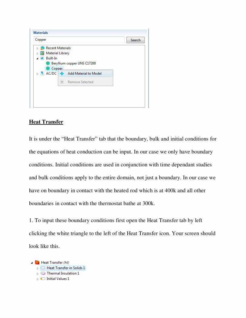
Heat Transfer

It is under the “Heat Transfer” tab that the boundary, bulk and initial conditions for

the equations of heat conduction can be input. In our case we only have boundary

conditions. Initial conditions are used in conjunction with time dependant studies

and bulk conditions apply to the entire domain, not just a boundary. In our case we

have on boundary in contact with the heated rod which is at 400k and all other

boundaries in contact with the thermostat bathe at 300k.

1. To input these boundary conditions first open the Heat Transfer tab by left

clicking the white triangle to the left of the Heat Transfer icon. Your screen should

look like this.

2. Right click the Heat Transfer icon to open a menu containing the various types

of bulk and boundary conditions. Go through this menu and select “Temperature”

by left clicking. A new icon will now appear under initial values that says

“Temperature” this is where we will input one of our two temperature conditions.

3. Add another temperature boundary condition by repeating step 2.

4. After adding the two temperature boundary

conditions your

screen should

look like the image to the right. We now

need to specify a value and a location for

our temperature boundary conditions. Let’s

start with the warm surface. Start by left

clicking “Temperature 1”. The interface

region of COMSOL should now look like

the image at left. We need to do 2 things

here. The first is to add the surface to which

we wish to apply this boundary condition and the second is to give a value to this

temperature. We will choose the bottom of our rectangle as the location for our

boundary condition. In the graphical interface left click this boundary (which

should then turn red as seen below and click the button to add. Now set the

temperature to 400 k by typing 400 into the To field.

If done properly your screen should look like this.

5. We now need to apply the cooler boundary condition. Do this by clicking

“Temperature 2” to open the interface and select the top and side boundaries to

apply the boundary condition. Then enter 300 into the To field. Your screen should

look the one below. This concludes our activities within the Heat Transfer tab we

can now proceed to calculate the solution.

Study

To calculate the solution to our PDE we simply right click on the “Study” tab and

click the green equals sign .

After solving the PDE the

temperature profile will be

displayed as shown below.

Results

To display the temperature at a given point left click the point you wish to probe

and the result will be displayed under the results tab as shown below.

To make a graph showing the temperature profile along a line we will need to add

a “cut line” to our solution and display the temperature along it. This may be done

as follows.

1. Right click “data sets” under the results

tab and select “2D cut line” from the

menu which will pop up.

2. The two points defining the “cut line”

need to be selected. In this case we will

have our “cut line” start at point (0.15,0) and end at point (0.15,0.05). To do this

enter these coordinates into

the “cut line 2D” screen

that will come up after left

clicking on the “Cut line

2D” icon under the data

sets tab. Your screen should

look like the one at left.

3. Press the paint brush button in the top right of the “Cut line 2D” screen to

have the cut line displayed. Your cut line should look like the one below.

4. We now need to add a “1D plot group” to the results. As you may be beginning

to realize COMSOL uses a right click

interface for addition of most options. So

right click “Results” and left click the “1D

plot group”.

5. We want to add a line graph to our “1D plot group”, so to do this right click on

“1D Plot Group” and choose

“Line Graph” from the menu.

This will add a line graph under the “1D plot group”

6. Finally left click on “Line graph” and for data select “Cut Line 2D”, this will

take the temperature everywhere

along the cut line we created. To

create the graph left click the paint

brush button . You should

obtain the following result.

As can be seen the temperature decreases linearly from the heated surface to the

cooled surface.

Adjusting The Problem

At this point it is a simple matter to go back and change some of our boundary or

bulk conditions. We will do so now.

We will start by changing the lateral surfaces to perfect insulators. We do this as

follows:

1. Go back to “Heat Transfer” and left click the arrow just to the right of this icon

to open all of the options.

2. Go to the boundary condition “Temperature 2” and de-select the lateral surfaces

so that now only the upper surface is at constant 300 k. You de-select a sub-

domain by left clicking it and then pressing the minus button . If done correctly

your constant temperature condition should look like the one below. By default

now the lateral surfaces will be insulated.

3. Right click on “Study” and press compute. The below result should appear.

Notice how only the region of the rectangle close to the lateral surfaces has

changed from before. If you check the temperature profile along the cut line you

shouldn’t see much of a change because this cut line was exactly in the middle of

our rectangle where the side effects were minimal.

We will now add a heat generation term. This is a bulk condition and can be added

in a similar way as the temperature boundary conditions.

1. Go back up to “Heat Transfer” and right click to open the list of possible

boundary and bulk conditions. Left click on

“Heat Source”, this will add a “Heat Source

1” icon within “Heat Transfer” menu. Left

click this to open the interface.

2. We need to add the domain over which this condition applies, and as a bulk

condition it will apply over the entire geometry. So left click the rectangle and then

left click the plus sign as done previously.

3. Now a value for a per volume heat generation term needs to be added. We will

use 100,000,000 W/m3

as shown below.

4. Again after changing any boundary or bulk condition(s) a new solution must be

found so right click on “Study” and press compute. The below result should be

obtained.

It is elucidating to examine the temperature profile for this solution so click on

your previously made line graph displaying the temperature across the cut line.

This should look like the one below.

Note how this differs from the solution without heat generation, the maximum

temperature is no longer at the heated surface, but instead near the center of the

rectangle because of the large amount of heat being produced throughout the entire

volume.

Example 1.1 (2D Axisymmetric Heat Transfer)

We will now solve the same problem as in example 1, but this time without the

reduction of the problem into rectangular coordinates. To avoid redundancy only

the steps that are significantly different from those in example 1 will be explained

in detail.

Startup

1. You will need to start a new model either be restarting COMSOL or by clicking

“New” in the “File” menu.

2. You will now select “2D Axisymmtric” instead

of simply 2D. This will take whatever geometry

you create and rotate it about an axis and is ideal

for problems with symmetry about an axis.

3. You will select “Heat Transfer” as your physics

and “Stationary” as your study as before.

Geometry

We will now create our geometry, this is the where the biggest differences exist

between this model and the previous one.

1. Right click geometry and add a rectangle.

2. Have the corner placed at z=0m and r=0.05m. Notice that our geometry will be

spun around the line r=0.

3. Click “Build All” and obtain the following result.

Materials

Select Copper as the material and apply this to the geometry as before.

Heat Transfer

We will use the same boundary conditions as before. Namely that

@ r=R1 T=400k

@ r=R2 T=300k

@ z=0 T=300k and @ z= 0.3m T=300k

This means that as before we will need to add two different temperature

conditions. This is done by right clicking on heat transfer and clicking temperature.

Enter the appropriate temperatures in the temperature field and select the

appropriate surfaces to apply these boundaries (same as before).

Study

Now that the model has been built we are ready to examine the solution. Right

click “Study” and left click compute. The below result should be obtained.

This is a pretty image but does not tell us much about the actual solution. To get a

better understanding of the temperature profile we will add a “Cut Line” as before.

1. Right click on “Data Sets” under the “Results” tab. Click “Cut Line 2D”

2. Set the two points for the cut line as (r=0.05m,z=0.15m) and (r=0.10,z=0.15m)

3. Right click on “Results” and add a 1D plot group.

4. Right click on 1D plot group and add a line graph.

5. In the line graph interface select “Cut line 2D” as the data source and click the

paintbrush icon to have the graph generated. The below result should be obtained.

Compare this solution to the solution from example 1.