Computing with Chunks - MIT...

Computing with Chunks

by

Justin Mazzola Paluska

S.B. PhysicsMassachusetts Institute of Technology (2003)

S.B. Electrical Engineering and Computer ScienceMassachusetts Institute of Technology (2003)

M.Eng. Electrical Engineering and Computer ScienceMassachusetts Institute of Technology (2004)

E.C.S. Electrical Engineering and Computer ScienceMassachusetts Institute of Technology (2012)

Submitted to the Department of Electrical Engineering and Computer Sciencein partial fulfillment of the requirements for the degree of

Doctor of Science

at the

MASSACHUSETTS INSTITUTE OF TECHNOLOGY

June 2013

© Massachusetts Institute of Technology 2013. All rights reserved.

Author . . . . . . . . . . . . . . . . . . . . . . . . . . . . . . . . . . . . . . . . . . . . . . . . . . . . . . . . . . . . . . . . . . . . . . . . . .Department of Electrical Engineering and Computer Science

May 22, 2013

Certified by . . . . . . . . . . . . . . . . . . . . . . . . . . . . . . . . . . . . . . . . . . . . . . . . . . . . . . . . . . . . . . . . . . . . . .Steve Ward

ProfessorThesis Supervisor

Accepted by . . . . . . . . . . . . . . . . . . . . . . . . . . . . . . . . . . . . . . . . . . . . . . . . . . . . . . . . . . . . . . . . . . . . .Leslie A. Kolodziejski

ProfessorChair, Department Committee on Graduate Students

Computing with Chunks

by

Justin Mazzola Paluska

Submitted to the Department of Electrical Engineering and Computer Scienceon May 22, 2013, in partial fulfillment of the

requirements for the degree ofDoctor of Science

Abstract

Modern computing substrates like general-purpose GPUs, massively multi-core processors,and cloud computing clusters offer practically unlimited resources at the cost of requir-ing programmers to manage those resources for correctness, efficiency, and performance.Instead of using generic abstractions to write their programs, programmers of moderncomputing substrates are forced to structure their programs around available hardware.This thesis argues for a new generic machine abstraction, the Chunk Model, that explicitlyexposes program and machine structure, making it easier to program modern computingsubstrates.

In the Chunk Model, fixed-sized chunks replace the flat virtual memories of traditionalcomputing models. Chunks may link to other chunks, preserving the structure of andimportant relationships within data and programs as an explicit graph of chunks. Sincechunks are limited in size, large data structures must be divided into many chunks, exposingthe structure of programs and data structures to run-time systems. Those run-time systems,in turn, may optimize run-time execution, both for ease of programming and performance,based on the exposed structure.

This thesis describes a full computing stack that implements the Chunk Model. At thebottom layer is a distributed chunk memory that exploits locality of hardware componentswhile still providing programmer-friendly consistency semantics and distributed garbagecollection. On top of the distributed chunk memory, we build a virtual machine that storesall run-time state in chunks, enabling computation to be distributed through the distributedchunk memory system. All of these features are aimed at making it easier to programmodern computing substrates.

This thesis evaluates the Chunk Model through example applications in cloud comput-ing, scientific computing, and shared client/server computing.

Thesis Supervisor: Steve WardTitle: Professor

3

Acknowledgments

During my quixotic journey through graduate school, I have been fortunate to have the

support of many caring and loving people. First, I would like to thank my advisor, Steve

Ward, for his advice and encouragement during my long tenure as a graduate student.

Steve’s many design and architecture insights helped shape the both the big picture ideas

and the implementation details of my thesis project. He has also helped me grow as an

engineer and as a scientist.

I acknowledge my thesis committee members, Anant Agarwal and Sam Madden, for

providing me with clear advice on how to clarify and improve my thesis. I appreciate all

of the warm advice Chris Terman has given me over the years, first as my undergraduate

advisor and later as a colleague. I also thank Cree Bruins for all of her help in fighting MIT’s

bureaucracy; I hope I have not caused too many problems!

I am deeply indebted to Hubert Pham for his continual help not only with my thesis

project, but also for being a close friend always willing to hear and help resolve complaints

and rants. I would not have been able to take on as many projects as I have in graduate

school without Hubert’s help.

I have been fortunate to work with many brilliant minds as project co-conspirators

and co-authors while at MIT: Christian Becker, Grace Chau, Brent Lagesse, Umar Saif,

Gregor Schiele, Chris Stawarz, Jacob Strauss, Jason Waterman, Eugene Weinstein, Victor

Williamson, and Fan Yang. I thank each of them for their input and expertise.

I thank my family for being my foundation and for their emotional support. To my

mom, thank you for teaching me to love learning and providing me with tools to succeed in

life. To my sister, thank you for showing me how to persevere though tough situations. To

my grandfather, thank you for always encouraging me. Finally, to Trisha, my partner in life,

I love you and thank you for growing with me as we both wound our ways through MIT.

5

This work was sponsored by the T-Party Project, a joint research program between MIT

and Quanta Computer Inc., Taiwan. Portions of this thesis were previously published at

IEEE PerCom [77], at HotOS [80], at ACM MCS [78], and in Pervasive and Mobile Comput-

ing [79]. The video frames used in Figures 2.1, 2.5, and 6.1 come from Elephants Dream [59]

and are used under the Creative Commons Attribution license.

6

Contents

1 Introduction 171.1 Program Structure versus Platform Structure . . . . . . . . . . . . . . . . . . 181.2 Mapping Structure . . . . . . . . . . . . . . . . . . . . . . . . . . . . . . . . . 20

1.2.1 Optimization within the Flat Middle . . . . . . . . . . . . . . . . . . . 201.2.2 Breaking the Abstraction . . . . . . . . . . . . . . . . . . . . . . . . . 211.2.3 Dissolving the Machine Abstraction . . . . . . . . . . . . . . . . . . . 22

1.3 Thesis: A Structured Computing Model . . . . . . . . . . . . . . . . . . . . . 231.3.1 Principles . . . . . . . . . . . . . . . . . . . . . . . . . . . . . . . . . . 231.3.2 Contributions . . . . . . . . . . . . . . . . . . . . . . . . . . . . . . . . 241.3.3 Thesis Outline . . . . . . . . . . . . . . . . . . . . . . . . . . . . . . . . 27

2 The Chunk Model 292.1 Chunks . . . . . . . . . . . . . . . . . . . . . . . . . . . . . . . . . . . . . . . . 312.2 Why Chunks? . . . . . . . . . . . . . . . . . . . . . . . . . . . . . . . . . . . . 32

2.2.1 Transparent and Generic Structure . . . . . . . . . . . . . . . . . . . . 322.2.2 Identities Instead of Addresses . . . . . . . . . . . . . . . . . . . . . . 332.2.3 Fixed Sizes . . . . . . . . . . . . . . . . . . . . . . . . . . . . . . . . . . 342.2.4 Chunk Parameters . . . . . . . . . . . . . . . . . . . . . . . . . . . . . 35

2.3 Example Chunk Structures . . . . . . . . . . . . . . . . . . . . . . . . . . . . . 362.3.1 ChunkStream: Chunks for Video . . . . . . . . . . . . . . . . . . . . . 362.3.2 CVM: Computing with Chunks . . . . . . . . . . . . . . . . . . . . . . 39

3 The Chunk Platform 453.1 Chunk Platform Overview . . . . . . . . . . . . . . . . . . . . . . . . . . . . . 453.2 The Chunk API and Memory Model . . . . . . . . . . . . . . . . . . . . . . . 48

3.2.1 API Usage . . . . . . . . . . . . . . . . . . . . . . . . . . . . . . . . . . 483.2.2 Memory Model . . . . . . . . . . . . . . . . . . . . . . . . . . . . . . . 50

3.3 Chunk Runtime . . . . . . . . . . . . . . . . . . . . . . . . . . . . . . . . . . . 513.3.1 Persistence . . . . . . . . . . . . . . . . . . . . . . . . . . . . . . . . . . 513.3.2 Runtime Hooks . . . . . . . . . . . . . . . . . . . . . . . . . . . . . . . 513.3.3 Chunk Libraries . . . . . . . . . . . . . . . . . . . . . . . . . . . . . . . 523.3.4 Chunk Peers and the Chunk Exchange Protocol . . . . . . . . . . . . 52

3.4 Reference Trees . . . . . . . . . . . . . . . . . . . . . . . . . . . . . . . . . . . 533.4.1 Sequential Consistency through Invalidation . . . . . . . . . . . . . . 543.4.2 Reference Tree Expansion . . . . . . . . . . . . . . . . . . . . . . . . . 583.4.3 Garbage Collection . . . . . . . . . . . . . . . . . . . . . . . . . . . . . 59

7

4 Taming the Chunk Exchange Protocol 634.1 Chunk Peer . . . . . . . . . . . . . . . . . . . . . . . . . . . . . . . . . . . . . 634.2 Distributed Reference Trees . . . . . . . . . . . . . . . . . . . . . . . . . . . . 644.3 Chunk Exchange Protocol Messages . . . . . . . . . . . . . . . . . . . . . . . 66

4.3.1 Message Structure and Nomenclature . . . . . . . . . . . . . . . . . . 664.4 Channel Layer and Channel Proxies . . . . . . . . . . . . . . . . . . . . . . . 68

4.4.1 Extending the Reference Tree . . . . . . . . . . . . . . . . . . . . . . . 694.4.2 Reference Tree Status Maintenance . . . . . . . . . . . . . . . . . . . . 72

4.5 Chunk Exchange Layer . . . . . . . . . . . . . . . . . . . . . . . . . . . . . . . 734.6 The Request Queue . . . . . . . . . . . . . . . . . . . . . . . . . . . . . . . . . 744.7 Chunk State . . . . . . . . . . . . . . . . . . . . . . . . . . . . . . . . . . . . . 754.8 The Reactor . . . . . . . . . . . . . . . . . . . . . . . . . . . . . . . . . . . . . 77

4.8.1 Expanding the Reference Tree . . . . . . . . . . . . . . . . . . . . . . . 804.8.2 Requesting Copies across the Reference Tree . . . . . . . . . . . . . . 814.8.3 Maintaining Sequential Consistency . . . . . . . . . . . . . . . . . . . 82

4.9 Garbage Collection . . . . . . . . . . . . . . . . . . . . . . . . . . . . . . . . . 844.9.1 Leaving the Reference Tree . . . . . . . . . . . . . . . . . . . . . . . . 854.9.2 Example . . . . . . . . . . . . . . . . . . . . . . . . . . . . . . . . . . . 884.9.3 Handling Loops . . . . . . . . . . . . . . . . . . . . . . . . . . . . . . . 90

5 Applications 935.1 SCVM . . . . . . . . . . . . . . . . . . . . . . . . . . . . . . . . . . . . . . . . . 93

5.1.1 The SCVM Virtual Machine Model . . . . . . . . . . . . . . . . . . . . 945.1.2 JSLite . . . . . . . . . . . . . . . . . . . . . . . . . . . . . . . . . . . . . 955.1.3 Photo Boss . . . . . . . . . . . . . . . . . . . . . . . . . . . . . . . . . . 98

5.2 Tasklets . . . . . . . . . . . . . . . . . . . . . . . . . . . . . . . . . . . . . . . . 1005.2.1 Tasklet Accounting with Chunks . . . . . . . . . . . . . . . . . . . . . 1015.2.2 Trading Tasklets . . . . . . . . . . . . . . . . . . . . . . . . . . . . . . . 102

5.3 ChunkStream . . . . . . . . . . . . . . . . . . . . . . . . . . . . . . . . . . . . 1035.3.1 Codec Considerations . . . . . . . . . . . . . . . . . . . . . . . . . . . 1035.3.2 Multimedia and Parallel Streams . . . . . . . . . . . . . . . . . . . . . 106

6 Chunk-based Optimization 1076.1 Experimental Setup . . . . . . . . . . . . . . . . . . . . . . . . . . . . . . . . . 1076.2 Server-side Paths . . . . . . . . . . . . . . . . . . . . . . . . . . . . . . . . . . 1086.3 Chunk Graph Pre-fetching . . . . . . . . . . . . . . . . . . . . . . . . . . . . . 110

7 Related Work 1157.1 Architectures . . . . . . . . . . . . . . . . . . . . . . . . . . . . . . . . . . . . . 1157.2 Object Systems and Garbage Collection . . . . . . . . . . . . . . . . . . . . . 1167.3 Operating Systems . . . . . . . . . . . . . . . . . . . . . . . . . . . . . . . . . 1187.4 Code Offload and Migration . . . . . . . . . . . . . . . . . . . . . . . . . . . . 1197.5 Pre-fetching . . . . . . . . . . . . . . . . . . . . . . . . . . . . . . . . . . . . . 1207.6 Tasklet Economic Models . . . . . . . . . . . . . . . . . . . . . . . . . . . . . 1207.7 Persistent Programming Systems . . . . . . . . . . . . . . . . . . . . . . . . . 1217.8 Locality-aware Re-structuring . . . . . . . . . . . . . . . . . . . . . . . . . . . 1227.9 Video Streaming . . . . . . . . . . . . . . . . . . . . . . . . . . . . . . . . . . . 122

8

8 Summary and Future Work 1258.1 Future Work . . . . . . . . . . . . . . . . . . . . . . . . . . . . . . . . . . . . . 127

8.1.1 High Performance Chunk Platform . . . . . . . . . . . . . . . . . . . 1278.1.2 Reference Tree Reliability . . . . . . . . . . . . . . . . . . . . . . . . . 1278.1.3 Migration of Computation . . . . . . . . . . . . . . . . . . . . . . . . . 127

8.2 Concluding Remarks . . . . . . . . . . . . . . . . . . . . . . . . . . . . . . . . 128

A Reactor Transition Pseudo-code 129

B SCVM Specification 133B.1 SCVM Programming Environment . . . . . . . . . . . . . . . . . . . . . . . . 133

B.1.1 Threads . . . . . . . . . . . . . . . . . . . . . . . . . . . . . . . . . . . 134B.1.2 Environments . . . . . . . . . . . . . . . . . . . . . . . . . . . . . . . . 134B.1.3 Closures and Functions . . . . . . . . . . . . . . . . . . . . . . . . . . 135B.1.4 Constants . . . . . . . . . . . . . . . . . . . . . . . . . . . . . . . . . . 136

B.2 SCVM Instructions . . . . . . . . . . . . . . . . . . . . . . . . . . . . . . . . . 136B.2.1 Stack Manipulation Instructions . . . . . . . . . . . . . . . . . . . . . 136B.2.2 Chunk Manipulation Instructions . . . . . . . . . . . . . . . . . . . . 137B.2.3 Integer Instructions . . . . . . . . . . . . . . . . . . . . . . . . . . . . . 138B.2.4 Comparison Instructions . . . . . . . . . . . . . . . . . . . . . . . . . . 139B.2.5 Boolean Instructions . . . . . . . . . . . . . . . . . . . . . . . . . . . . 139B.2.6 Function Instructions . . . . . . . . . . . . . . . . . . . . . . . . . . . . 139

B.3 Warts . . . . . . . . . . . . . . . . . . . . . . . . . . . . . . . . . . . . . . . . . 140

C Big Jacobi Source Code 141

9

List of Figures

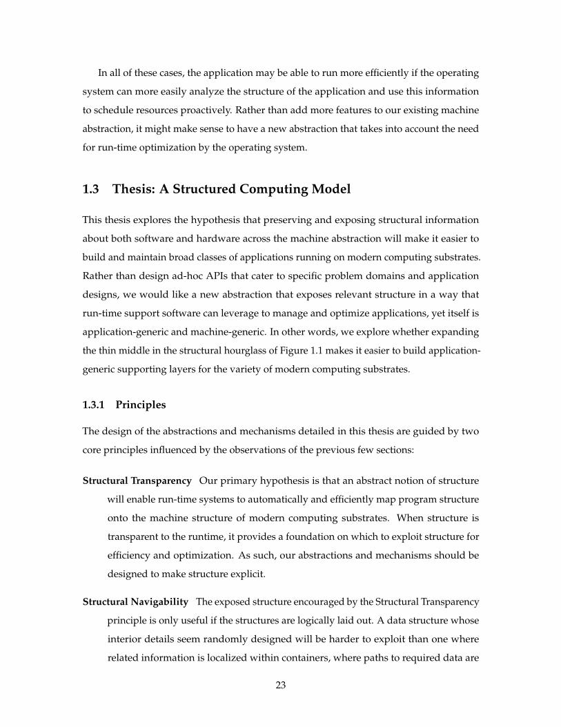
1.1 The structural hourglass of computing. . . . . . . . . . . . . . . . . . . . . . 19

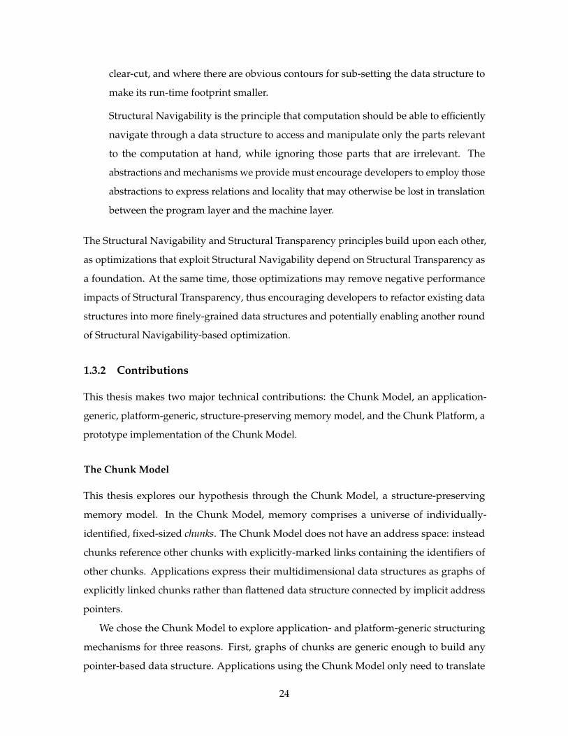
1.2 A universe of chunks divided into finite subsets. . . . . . . . . . . . . . . . . 25

2.1 Comparison of the traditional flat-memory model and the Chunk Model. . 30

2.2 Two chunks with a link between them. . . . . . . . . . . . . . . . . . . . . . . 31

2.3 A large image spills over into multiple chunks. . . . . . . . . . . . . . . . . . 32

2.4 Alternative chunk structures for storing image data. . . . . . . . . . . . . . . 35

2.5 Chunk-based video stream representation used by ChunkStream. . . . . . . 37

2.6 CVM Data Structure . . . . . . . . . . . . . . . . . . . . . . . . . . . . . . . . 40

2.7 Volumes of influence for three threads. . . . . . . . . . . . . . . . . . . . . . . 42

3.1 Overview of the Chunk Platform. . . . . . . . . . . . . . . . . . . . . . . . . . 46

3.2 Architectural diagram of the Chunk Platform. . . . . . . . . . . . . . . . . . 47

3.3 Access privileges of the Chunk API Memory Model . . . . . . . . . . . . . . 50

3.4 A simple data structure distributed over six Chunk Peers. . . . . . . . . . . . 52

3.5 Reference Tree for Figure 3.4. . . . . . . . . . . . . . . . . . . . . . . . . . . . 54

3.6 Reference Tree configuration needed to grant a Modify privilege. . . . . . . 55

3.7 A race between two Modify privilege requests. . . . . . . . . . . . . . . . . . 57

3.8 An example of Reference Tree expansion. . . . . . . . . . . . . . . . . . . . . 58

3.9 Garbage collection example. . . . . . . . . . . . . . . . . . . . . . . . . . . . . 61

4.1 Distributed Reference Tree state. . . . . . . . . . . . . . . . . . . . . . . . . . 65

4.2 Chunk State as a copy moves to another node. . . . . . . . . . . . . . . . . . 71

4.3 The components of the Chunk Exchange layer. . . . . . . . . . . . . . . . . . 74

4.4 Chunk and Channel States during Reference Tree expansion. . . . . . . . . . 80

4.5 Chunk and Channel States when node 1 requests a copy of the chunk. . . . 81

11

4.6 Chunk and Channel States for the process of granting a Modify request. . . 83

4.7 The T bit protects against premature collection of sub-graphs of chunks. . . 87

4.8 Garbage collection example for a node with no chunk copy. . . . . . . . . . . 88

4.9 Garbage collection example for a node with a chunk copy. . . . . . . . . . . 89

4.10 A cycle spanning multiple nodes. . . . . . . . . . . . . . . . . . . . . . . . . . 91

5.1 The SCVM ecosystem. . . . . . . . . . . . . . . . . . . . . . . . . . . . . . . . 94

5.2 SCVM bytecode for factorial(n). . . . . . . . . . . . . . . . . . . . . . . . . . . 96

5.3 Screen shot of the Quickr photo organization tool. . . . . . . . . . . . . . . . 99

5.4 Screen shot of the PhotoChop photo editing tool. . . . . . . . . . . . . . . . . 99

5.5 Tasklet Trading Service . . . . . . . . . . . . . . . . . . . . . . . . . . . . . . . 103

5.6 FrameContext chunks. . . . . . . . . . . . . . . . . . . . . . . . . . . . . . . . 105

6.1 Clients using server-side path de-referencing. . . . . . . . . . . . . . . . . . . 108

6.2 Data transferred streaming a video. . . . . . . . . . . . . . . . . . . . . . . . . 109

6.3 Radius Pre-fetching Performance. . . . . . . . . . . . . . . . . . . . . . . . . . 110

6.4 Shape Pre-fetching Performance. . . . . . . . . . . . . . . . . . . . . . . . . . 112

6.5 Late-arriving Pre-fetched Chunks. . . . . . . . . . . . . . . . . . . . . . . . . 113

12

List of Listings

2.1 Client-side playback algorithm for ChunkStream. . . . . . . . . . . . . . . . 38

4.1 (J?) Channel Proxy bootstrap procedures. . . . . . . . . . . . . . . . . . . . . 70

4.2 B? Channel Proxy bootstrap procedures. . . . . . . . . . . . . . . . . . . . . . 70

A.1 The FC Transition. . . . . . . . . . . . . . . . . . . . . . . . . . . . . . . . . . . 130

A.2 The FE Transition. . . . . . . . . . . . . . . . . . . . . . . . . . . . . . . . . . . 130

A.3 The RQC Transition. . . . . . . . . . . . . . . . . . . . . . . . . . . . . . . . . 130

A.4 The RQE Transition. . . . . . . . . . . . . . . . . . . . . . . . . . . . . . . . . . 130

A.5 The RSC Transition. . . . . . . . . . . . . . . . . . . . . . . . . . . . . . . . . . 130

A.6 The RSE Transition. . . . . . . . . . . . . . . . . . . . . . . . . . . . . . . . . . 131

A.7 The FRSE Transition . . . . . . . . . . . . . . . . . . . . . . . . . . . . . . . . 131

A.8 The GRR Transition. . . . . . . . . . . . . . . . . . . . . . . . . . . . . . . . . 131

A.9 The GRM Transition. . . . . . . . . . . . . . . . . . . . . . . . . . . . . . . . . 132

A.10 The GCLT Transition. . . . . . . . . . . . . . . . . . . . . . . . . . . . . . . . . 132

A.11 The GCD Transition. . . . . . . . . . . . . . . . . . . . . . . . . . . . . . . . . 132

A.12 The GCRG Transition. . . . . . . . . . . . . . . . . . . . . . . . . . . . . . . . 132

C.1 big_jacobi.js . . . . . . . . . . . . . . . . . . . . . . . . . . . . . . . . . . . . . . 141

13

List of Tables

3.1 Chunk API exposed by the Chunk Runtime. . . . . . . . . . . . . . . . . . . 49

4.1 Chunk Exchange Protocol Request messages. . . . . . . . . . . . . . . . . . . 67

4.2 Chunk Exchange Protocol status messages. . . . . . . . . . . . . . . . . . . . 68

4.3 The Channel States of the Chunk Exchange Protocol. . . . . . . . . . . . . . 69

4.4 Transition table of the Channel Proxy FSM. . . . . . . . . . . . . . . . . . . . 72

4.5 The six types of requests. . . . . . . . . . . . . . . . . . . . . . . . . . . . . . . 74

4.6 Major Chunk State bits . . . . . . . . . . . . . . . . . . . . . . . . . . . . . . . 75

4.7 Privilege bits . . . . . . . . . . . . . . . . . . . . . . . . . . . . . . . . . . . . . 75

4.8 The Reactor reaction table. . . . . . . . . . . . . . . . . . . . . . . . . . . . . . 78

4.9 Reactor function descriptions. . . . . . . . . . . . . . . . . . . . . . . . . . . . 79

4.10 Reactor Error Types . . . . . . . . . . . . . . . . . . . . . . . . . . . . . . . . . 80

6.1 Table of raw Radius Pre-fetch performance values. . . . . . . . . . . . . . . . 111

6.2 Shape Table for Elephants Dream. . . . . . . . . . . . . . . . . . . . . . . . . . 111

6.3 Table of raw Shape Pre-fetch performance values. . . . . . . . . . . . . . . . 113

15

Chapter 1

Introduction

In the past few years, the computer industry has seen the growth of three new computing

substrates: elastic cloud computing, massively multi-core computing, and general-purpose

GPU computing. At a high-level, these three substrates are wildly different. Elastic cloud

computing systems like Amazon’s EC2 [8] and Microsoft’s Azure [70] provide dynamically

expandable clusters of hosts, each connected over a virtualized network. Massively multi-

core processors like the Tilera TILE [91] series of processors provide a plethora of processor

cores connected by on-chip buses and local caches. General-purpose GPUs like NVIDIA’s

Tesla [64] provide an abundance of ALUs connected by a hierarchy of memories.

While the granularity and specifics of these new substrates differ, what is common to all

of them is (1) an abundance of processing elements and (2) programmer-visible communi-

cation and storage hierarchies whose proper utilization determines both correctness and

performance of applications. For example, in the cloud, intra-core operations are faster than

intra-host operations, which are faster than inter-host operations. Likewise, in the GPU,

communication and data sharing within a single processing element is fast compared to

communication and sharing processing between elements, which itself is fast compared to

CPU to GPU communication.

In contrast to “normal” CPU-based platforms that automatically manage the memory

and communication hierarchy for correctness and high performance, programmers must

carefully manage the communications and storage hierarchies of the new computing sub-

strates so that processing elements are continually fed with instructions and data. Typically

this is done by manually managing communication and data placement with substrate-

17

specific frameworks to ensure that related computations are on processing elements close to

each other in the computing substrate and that computations “fit” into the variously sized

storage buckets that each level of the substrate provides. The substrate-specific frameworks

force programmers to use special programming paradigms that chain their programs to

particular configurations of specific machines. This is unfortunate because it takes flexibility

away from programmers by restricting how they may solve their problems.

1.1 Program Structure versus Platform Structure

To better understand the predicament of modern computing substrates, it is instructive to

review how software and hardware are structured and how they work together. At the

programming-language layer, programmers use structuring mechanisms provided by their

favorite language to construct models of the real-world problems they need to solve. For

example, all programming languages provide functions to organize algorithms and control

execution of code as well as record types to organize related data. Functions can be further

decomposed into basic blocks connected by explicit flow control primitives. Object-oriented

languages extend the model by providing objects that tie code and related methods together.

At this top-layer, programming language structuring mechanisms allow programmers

to optimize for maintainability and readability of code by keeping related concepts near

each other in source code—leading to locality of concepts in the program source—as well

as build layers of abstraction that hide unnecessary details that would otherwise hinder

understanding of the program.

Explicit structure is also rich at the hardware layer. At this level, structure reflects

finite physical resources with different performance characteristics, sizes, and availability.

For example, memory is organized into a hierarchy of fast and small caches spilling over

into multi-channel DRAM main-memories, all backed by slow, but potentially enormous,

disks and network file systems. Data that are in the same cache will be equally fast to

access, while those that are in different levels of the hierarchy will have slower access

times. A program whose working set can fit within a high-speed cache will be orders of

magnitude faster than a program that must go out to main memory, or worse yet, swap.

Similarly, computation power is organized into threads that execute on particular cores

embedded within a heterogeneous communication topology. Two threads assigned to the

18

same processor or chip package will be able to more easily communicate and synchronize

than two threads in cores in different places on the network. Similarly, threads on the same

network will be able to more easily communicate and synchronize compared to threads

that must communicate over the wide-area Internet. In general, the closer two related

items are to each other in the memory or processor network, the faster the application will

be able to combine and use the items. However, cost and power concerns constrain the

fast components to be small relative to the rest of the system, forcing the application and

operating system to continually copy data into and out of the fast components in order

to maintain high performance. Ergo, the hardware has a natural, if non-linear, “distance”

metric between components.

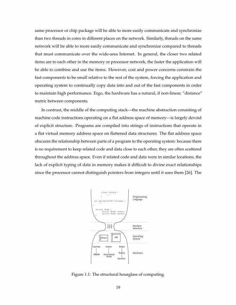
In contrast, the middle of the computing stack—the machine abstraction consisting of

machine code instructions operating on a flat address space of memory—is largely devoid

of explicit structure. Programs are compiled into strings of instructions that operate in

a flat virtual memory address space on flattened data structures. The flat address space

obscures the relationship between parts of a program to the operating system: because there

is no requirement to keep related code and data close to each other, they are often scattered

throughout the address space. Even if related code and data were in similar locations, the

lack of explicit typing of data in memory makes it difficult to divine exact relationships

since the processor cannot distinguish pointers from integers until it uses them [26]. The

MachineInterface

ProgrammingLanguage

OperatingSystem

Hardware

class Person { ...}

int decode(FILE *stream) { ...}

struct Node { struct Node *next; struct Node *prev;}

VMProcs

Caches

DRAM

DisksCores

FunctionalUnits

Tracks

Sectors

Figure 1.1: The structural hourglass of computing.

19

flat address space also obscures from the program the costs of different data structures and

code organizations since the machine model offers no portable way of exposing the sizes,

and consequently, the predicted placement or fragmentation of objects within the hardware

components in the system. As Figure 1.1 illustrates, the machine abstraction forms the

structural bottleneck between the highly structured ends of hardware and software.

1.2 Mapping Structure

Since compute resources are of finite size and there is a cost associated with moving

data between different components of the machine, a key problem in maintaining high

performance in a computer system is ensuring that related parts of a program are located

“close” to each other. When resource characteristics and limits are known, e.g., exactly

how big a component can get before it overflows a level in the storage hierarchy or exactly

how close two related threads of computation need to be to maintain high performance,

programmers can build systems that exploit resources efficiently. For example, once a

spinning hard disk has positioned its disk read head over a track, it can read or write the

entire track at very high speed, but will not be able to perform any reads or writes while

moving (seeking) the head to another track. As such, file systems have evolved to collect

many small reads and writes and coalesce them into a single large read or write to avoid

costly head seeks.

1.2.1 Optimization within the Flat Middle

Given that both programs and computers are highly structured, we would like to cast the

locality problem to one of mapping program structure onto machine structure, ideally in

a machine-portable way. Unfortunately, the unstructured machine abstraction makes the

mapping harder since program structure is obscured by the implicit structure of machine

code and the machine’s structure is obscured by the flat memory address space. Indeed,

it is because of how the traditional machine abstraction obscures structure that modern

computing substrates each come with their own frameworks and structuring abstractions.

The design choice to connect two highly structured layers with an unstructured inter-

mediary layer made sense at one time because the two layers have orthogonal structure

and could be engineered independently. Indeed, for the past several decades, computer

20

scientists and engineers have been able to build elegant optimizations at each end of our

hourglass that provided acceptable performance despite the thin middle. At the hardware-

level, caches trace program execution and place commonly used code and data in fast

memory banks close to the processor, essentially dynamically extracting “close” code and

data from patterns in the memory access stream. At the software layer, optimizing compil-

ers remove unnecessary structure from applications by putting related code in the same

basic blocks. The flattened code essentially groups related functions into sequential streams

of instructions, better matching the cache-enhanced flat execution environment by enabling

address-based caches to pre-fetch more related data.

1.2.2 Breaking the Abstraction

These optimizations, however, can only extract so much structure from the executing

program. As computers evolved, simple caches and hardware-agnostic optimizations were

no longer good enough to fully utilize new hardware and the industry resorted to breaking

through the clean machine code abstraction.

For example, in the early 1990’s compilers were tuned for the pipelines, delay slots,

and cache configuration for specific processors [22, 93], leaking specific hardware details

through the machine language abstraction up to the program and, consequently, pairing

binaries to specific implementation details of particular machines. Recent work on cache-

oblivious algorithms and data structures [37] has reduced the need to worry about the

specifics of any cache—though cache-oblivious algorithms do assume that there is some

hierarchy in the memory system. Demaine [30] surveys early work in the area and shows

that for many problems, cache-oblivious algorithms can meet the theoretical running times

of cache-aware algorithms. Unfortunately, cache-oblivious algorithms require program

code to be structured in a particular way that limits how programmers may implement

their algorithms.

Similarly, very long instruction word (VLIW) processors [35] expose all of the functional

units in the processor directly to the user program and require the user program (or

compiler) to schedule everything. VLIW failed in the marketplace for two reasons. First,

each VLIW processor had a different number of functional units, and as such required

different binaries for each generation of the same processor family, reducing portability.

21

Second, compilers could not statically fill functional units any better than normal super-

scalar processors.

1.2.3 Dissolving the Machine Abstraction

The systems of the previous section all break the machine abstraction by exposing low-

level information to the highest levels of the computation stack, where it was believed

that a compiler could make the most use of the extra information. However, these fix-

ups are unsuccessful because there is only so much optimization that can be applied to

the instruction stream of a single program. As the computing environment continues to

evolve, we may be faced with problems that may not be solvable by simply considering

a single stream of instructions, but rather may require a more holistic approach to how

applications are structured and how they may interact with increasingly complex machines.

For example:

• Users increasingly interact with video and other streaming media that passes through

the processor once, suffering high memory latencies to bring data into the processor

as well as polluting the cache with now-stale data. The program may work more

efficiently if the processor pre-fetches data into a reserved subset of cache lines while

leaving other lines alone. In order to do so, we need a way to analyze the structure of

the streaming media application and have a run-time system schedule memory reads

ahead of the application.

• As processor frequency scaling has hit a power-induced limit, we have seen a resur-

gence in distributed and parallel computing. In the flat model, the program must

manage its own execution and manage the lifetime of threads. Programmers would

be far more efficient if the system could identify program areas that may potentially

run in parallel and use that information to automatically manage thread pools for the

application.

• Many modern applications also make use of computing clusters that scatter parts of

the application across many machines. Is there a way to allow a run-time system to

optimize placement of components based on the dynamic needs of applications?

22

In all of these cases, the application may be able to run more efficiently if the operating

system can more easily analyze the structure of the application and use this information

to schedule resources proactively. Rather than add more features to our existing machine

abstraction, it might make sense to have a new abstraction that takes into account the need

for run-time optimization by the operating system.

1.3 Thesis: A Structured Computing Model

This thesis explores the hypothesis that preserving and exposing structural information

about both software and hardware across the machine abstraction will make it easier to

build and maintain broad classes of applications running on modern computing substrates.

Rather than design ad-hoc APIs that cater to specific problem domains and application

designs, we would like a new abstraction that exposes relevant structure in a way that

run-time support software can leverage to manage and optimize applications, yet itself is

application-generic and machine-generic. In other words, we explore whether expanding

the thin middle in the structural hourglass of Figure 1.1 makes it easier to build application-

generic supporting layers for the variety of modern computing substrates.

1.3.1 Principles

The design of the abstractions and mechanisms detailed in this thesis are guided by two

core principles influenced by the observations of the previous few sections:

Structural Transparency Our primary hypothesis is that an abstract notion of structure

will enable run-time systems to automatically and efficiently map program structure

onto the machine structure of modern computing substrates. When structure is

transparent to the runtime, it provides a foundation on which to exploit structure for

efficiency and optimization. As such, our abstractions and mechanisms should be

designed to make structure explicit.

Structural Navigability The exposed structure encouraged by the Structural Transparency

principle is only useful if the structures are logically laid out. A data structure whose

interior details seem randomly designed will be harder to exploit than one where

related information is localized within containers, where paths to required data are

23

clear-cut, and where there are obvious contours for sub-setting the data structure to

make its run-time footprint smaller.

Structural Navigability is the principle that computation should be able to efficiently

navigate through a data structure to access and manipulate only the parts relevant

to the computation at hand, while ignoring those parts that are irrelevant. The

abstractions and mechanisms we provide must encourage developers to employ those

abstractions to express relations and locality that may otherwise be lost in translation

between the program layer and the machine layer.

The Structural Navigability and Structural Transparency principles build upon each other,

as optimizations that exploit Structural Navigability depend on Structural Transparency as

a foundation. At the same time, those optimizations may remove negative performance

impacts of Structural Transparency, thus encouraging developers to refactor existing data

structures into more finely-grained data structures and potentially enabling another round

of Structural Navigability-based optimization.

1.3.2 Contributions

This thesis makes two major technical contributions: the Chunk Model, an application-

generic, platform-generic, structure-preserving memory model, and the Chunk Platform, a

prototype implementation of the Chunk Model.

The Chunk Model

This thesis explores our hypothesis through the Chunk Model, a structure-preserving

memory model. In the Chunk Model, memory comprises a universe of individually-

identified, fixed-sized chunks. The Chunk Model does not have an address space: instead

chunks reference other chunks with explicitly-marked links containing the identifiers of

other chunks. Applications express their multidimensional data structures as graphs of

explicitly linked chunks rather than flattened data structure connected by implicit address

pointers.

We chose the Chunk Model to explore application- and platform-generic structuring

mechanisms for three reasons. First, graphs of chunks are generic enough to build any

pointer-based data structure. Applications using the Chunk Model only need to translate

24

Figure 1.2: A universe of chunks divided into finite subsets. Each subset may be hosted byindependent machines. Note that some links extend beyond the borders of the figure.

their internal structures to chunk-based ones, rather than use platform-specific structuring

primitives. Second, the Chunk Model forces objects larger than one chunk to be expressed

as graphs of chunks. In doing so, the application explicitly exposes its structures to run-time

layers, enabling those run-time layers to optimize execution of the chunk-based applications

using information in the chunk graph. Third, the use of identities rather than addresses

insulates the Chunk Model from the constraints of any platform-specific addressing scheme.

As shown in Figure 1.2, it is possible to divide the universe into bounded, potentially shared,

subsets of chunks distributed among independent hardware nodes. While a particular piece

of hardware may only be able to access its finite subset of the universe of chunks at any given

time, clever management and translation of “universal identities” to local identifiers ensure

that nodes using the Chunk Model may migrate chunks between themselves, enabling each

node to have a finite window on the infinite universe of chunks.

The Chunk Platform

The Chunk Platform implements the Chunk Model while embracing the distributed and

network-oriented nature of modern computing substrates. Each node in the Chunk Platform

runs a node-local Chunk Runtime that manages the chunk-based applications on the node

and provides those applications with a Chunk API that give them a window into the

universe of shared chunks.

25

The Chunk Runtime on each node can only hold a subset of the shared universe of

chunks. To give applications access to the whole universe of chunks, the Chunk Runtime

on each node uses a low-level networking protocol called the Chunk Exchange Protocol to

manage the distribution of chunks. The Chunk Exchange Protocol enables nodes to divvy

up the universe of chunks among Chunk Runtimes, as illustrated by Figure 1.2. The Chunk

Runtime uses the Chunk Exchange Protocol to take care of coherent caching of chunks,

consistent updates to chunk copies, and reclamation of chunks as computations no longer

need them. The Chunk Exchange Protocol uses Reference Trees, an abstraction introduced

by Halstead [47], to manage chunks distributed across multiple Chunk Runtimes. Reference

Trees abstract and summarize the configuration of the distributed chunk universe in a way

that reduces the amount of local state each Chunk Runtime must maintain. Reference Trees

also provide convenient mechanisms for maintaining consistency of chunk updates as well

as for garbage collection of chunk resources.

The Chunk Platform serves as a prototyping platform to evaluate and validate the

Chunk Model. As such, the Chunk Platform supports a variety of applications ranging

from those that use chunks only as a distributed data store to SCVM, a virtual machine

architecture that uses the Chunk Model for computation.

Other Contributions

While we primarily use the Chunk Platform to evaluate the Chunk Model, our implementa-

tion of the Chunk Platform provides several other contributions:

• a wire format for sharing graphs of chunks,

• a distributed protocol implementing a sequentially consistent memory model for

shared graphs of chunks,

• a distributed garbage collection algorithm of chunk graphs that can collect cycles

distributed across many nodes,

• a reference compiler that targets chunks while hiding the chunk model from the

programmer, and

• a new model for sharing small “tasklets” among clients and servers in the cloud.

26

In most cases, while these contributions make use of our particular chunk abstraction,

they can be adapted to traditional reference-based object systems and thus are useful

independent of the Chunk Platform.

1.3.3 Thesis Outline

The next chapter details the Chunk Model. Chapter 3 outlines the Chunk Platform at a high

level. A lower-level description of the Chunk Platform, including details of its application-

generic run-time services, consistency model, and garbage collection algorithm, follows

in Chapter 4. Chapters 5 and 6 evaluate the Chunk Platform through building chunk-

based applications and evaluating chunk-based optimization techniques, respectively. After

evaluation, the thesis continues with a review of related work in Chapter 7 and concludes

with future work in Chapter 8.

27

Chapter 2

The Chunk Model

This thesis explores the Chunk Model as a more structured replacement for the unstructured

memory abstraction of current computing models. The Chunk Model extends the standard

von Neumann approach to computing with a structured memory rather than a flat memory.

In doing so, the Chunk Model enables a structured way of storing everything, from data to

computer programs to the run-time state of those programs.

The Chunk Model differs from the current flat memory abstraction in three ways.

First, the Chunk Model replaces memory as a flat array of bytes with an unbounded

universe of chunks. Chunks are fixed-size, so large data structures must be represented as

graphs of many inter-referencing chunks. These graphs embody the Structural Transparency

Principle and enable the Chunk Model to capture application-specific structure in a generic

way.

Second, the Chunk Model replaces pointer arithmetic as a way of navigating memory

with de-referencing explicitly-typed links between chunks. Chunks in the Chunk Model

have identities, not addresses; the only notion of distance between chunks stems from

the links between them rather than the nearness of addresses. Explicit links serve our

transparency goal, since it allows run-time services to read graphs of chunks without

complex analysis to disambiguate integers from pointers, while requiring chunk identities

force the use of links to identify chunks, since there is no way to obtain a chunk except by

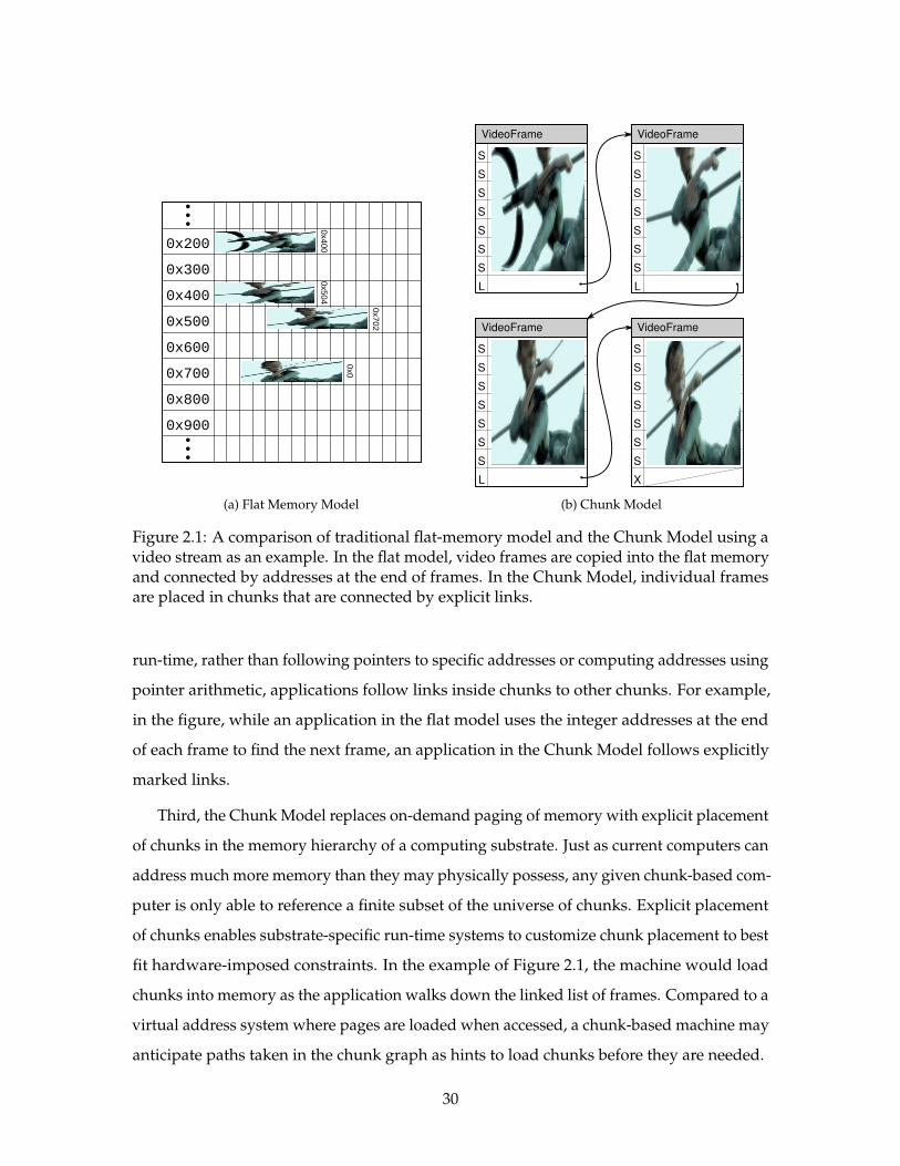
de-referencing a chunk identifier. As Figure 2.1 illustrates with the last four frames of a

video, rather than placing arbitrary data as a monolithic binary in the flat memory address

space, the Chunk Model compels applications to place their data in a graph of chunks. At

29

•••

0x200

0x300

0x400

0x500

0x600

0x700

0x800

0x900

•••

0x400

0x504

0x702

0x0

(a) Flat Memory Model

S

S

S

S

S

S

S

L

VideoFrame

S

S

S

S

S

S

S

L

VideoFrame

S

S

S

S

S

S

S

L

VideoFrame

S

S

S

S

S

S

S

X

VideoFrame

(b) Chunk Model

Figure 2.1: A comparison of traditional flat-memory model and the Chunk Model using avideo stream as an example. In the flat model, video frames are copied into the flat memoryand connected by addresses at the end of frames. In the Chunk Model, individual framesare placed in chunks that are connected by explicit links.

run-time, rather than following pointers to specific addresses or computing addresses using

pointer arithmetic, applications follow links inside chunks to other chunks. For example,

in the figure, while an application in the flat model uses the integer addresses at the end

of each frame to find the next frame, an application in the Chunk Model follows explicitly

marked links.

Third, the Chunk Model replaces on-demand paging of memory with explicit placement

of chunks in the memory hierarchy of a computing substrate. Just as current computers can

address much more memory than they may physically possess, any given chunk-based com-

puter is only able to reference a finite subset of the universe of chunks. Explicit placement

of chunks enables substrate-specific run-time systems to customize chunk placement to best

fit hardware-imposed constraints. In the example of Figure 2.1, the machine would load

chunks into memory as the application walks down the linked list of frames. Compared to a

virtual address system where pages are loaded when accessed, a chunk-based machine may

anticipate paths taken in the chunk graph as hints to load chunks before they are needed.

30

Grand Teton Nat

ional Park is l

ocated in north

western Wyoming

, south of Yell

owstone Nationa

l Park. The pa

S

S

S

S

S

S

S

L

TextChunk

S

S

S

S

S

S

S

S

ImageChunk

#73#163

#73

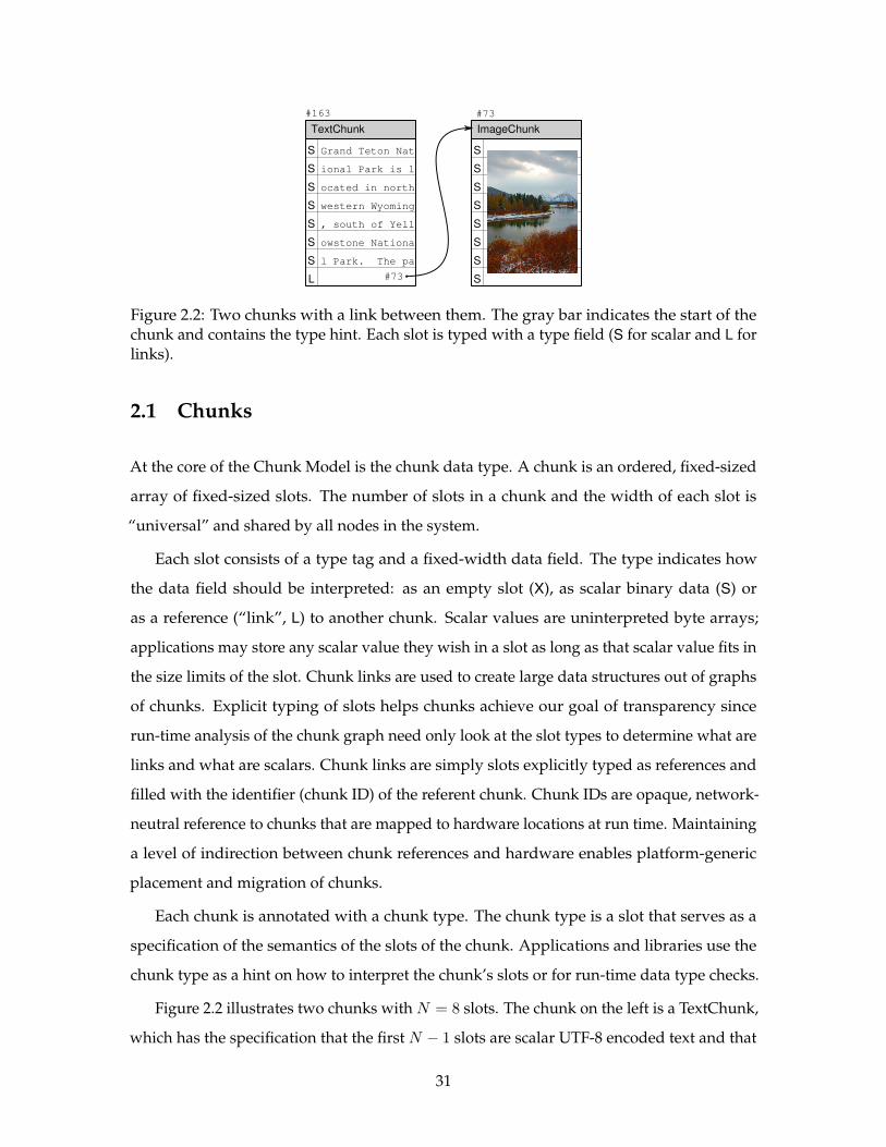
Figure 2.2: Two chunks with a link between them. The gray bar indicates the start of thechunk and contains the type hint. Each slot is typed with a type field (S for scalar and L forlinks).

2.1 Chunks

At the core of the Chunk Model is the chunk data type. A chunk is an ordered, fixed-sized

array of fixed-sized slots. The number of slots in a chunk and the width of each slot is

“universal” and shared by all nodes in the system.

Each slot consists of a type tag and a fixed-width data field. The type indicates how

the data field should be interpreted: as an empty slot (X), as scalar binary data (S) or

as a reference (“link”, L) to another chunk. Scalar values are uninterpreted byte arrays;

applications may store any scalar value they wish in a slot as long as that scalar value fits in

the size limits of the slot. Chunk links are used to create large data structures out of graphs

of chunks. Explicit typing of slots helps chunks achieve our goal of transparency since

run-time analysis of the chunk graph need only look at the slot types to determine what are

links and what are scalars. Chunk links are simply slots explicitly typed as references and

filled with the identifier (chunk ID) of the referent chunk. Chunk IDs are opaque, network-

neutral reference to chunks that are mapped to hardware locations at run time. Maintaining

a level of indirection between chunk references and hardware enables platform-generic

placement and migration of chunks.

Each chunk is annotated with a chunk type. The chunk type is a slot that serves as a

specification of the semantics of the slots of the chunk. Applications and libraries use the

chunk type as a hint on how to interpret the chunk’s slots or for run-time data type checks.

Figure 2.2 illustrates two chunks with N = 8 slots. The chunk on the left is a TextChunk,

which has the specification that the first N − 1 slots are scalar UTF-8 encoded text and that

31

S

S

S

S

S

S

S

L

ImageChunk

S

S

S

S

S

S

S

L

ImageChunk

S

S

S

S

S

S

S

L

ImageChunk

S

S

S

S

S

S

S

X

ImageChunk

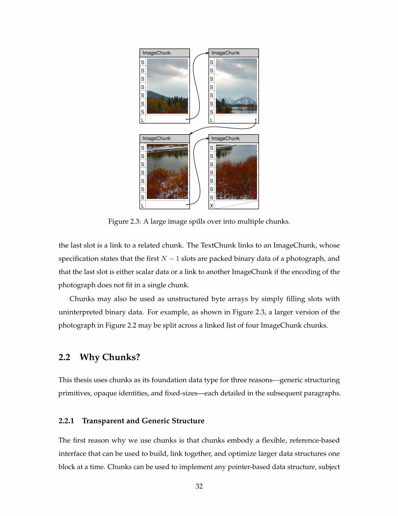
Figure 2.3: A large image spills over into multiple chunks.

the last slot is a link to a related chunk. The TextChunk links to an ImageChunk, whose

specification states that the first N − 1 slots are packed binary data of a photograph, and

that the last slot is either scalar data or a link to another ImageChunk if the encoding of the

photograph does not fit in a single chunk.

Chunks may also be used as unstructured byte arrays by simply filling slots with

uninterpreted binary data. For example, as shown in Figure 2.3, a larger version of the

photograph in Figure 2.2 may be split across a linked list of four ImageChunk chunks.

2.2 Why Chunks?

This thesis uses chunks as its foundation data type for three reasons—generic structuring

primitives, opaque identities, and fixed-sizes—each detailed in the subsequent paragraphs.

2.2.1 Transparent and Generic Structure

The first reason why we use chunks is that chunks embody a flexible, reference-based

interface that can be used to build, link together, and optimize larger data structures one

block at a time. Chunks can be used to implement any pointer-based data structure, subject

32

to the constraint that the largest single element fits in a single chunk. Small chunks force the

use of fine-grained data structures, creating many more decision, and optimization, points

over whether or not to fetch a particular portion of a data structure.

Since the chunk interface is fixed and chunk links are network-neutral references, chunk-

based data structures can be shared between any two nodes that use chunks without

worrying about format mismatches. The chunk abstraction and the chunk interface is the

embodiment of the Structural Transparency Principle of this thesis because chunks expose

structure through the graph induced by the explicitly marked links. System-level code—like

that handling coherence, caching, and optimization—can operate at and optimize the layers

underneath the application using only the structure exposed by chunks without needing to

worry about the exact semantics of each slot’s value.

2.2.2 Identities Instead of Addresses

The second reason for using chunks is that chunk IDs are opaque references and not

addresses. Opaque chunk IDs serve to break the abstraction of the flat virtual memory

address space as well as provide a level of indirection between chunks and the locations

where they are stored. The former is important because it removes the assumption that

virtual addresses near each other have anything to do with each other, a fallacy because

the contents of one virtual address may be in a L1 cache and available in a cycle while

the next word in the virtual memory may be on disk and take millions of cycles to fetch.

Breaking up a data structure into chunks makes it explicit that crossing a chunk boundary

may impose a performance hit. Moreover, address arithmetic no longer works, meaning

that data structures can only be accessed via paths in the chunk graph, rather than randomly.

Doing so exposes the true cost of data structures, since (1) it is necessary to build helper

chunks to access large data structures and (2) those data structures reflect, in chunk loads,

the costs of accessing random items in memory normally obscured by the virtual memory

subsystem.

The indirection property of opaque chunk IDs is important for two architectural reasons.

First, it enables chunks to be moved around not only between processes, but also between

nodes in the same network, giving a chunk-based run-time system the flexibility to not

only place chunks within the memory hierarchy of one node, but also to place chunks on

other nodes in the computation substrate. Second, using opaque chunk IDs frees the Chunk

33

Model from the inherent finiteness of an address-based namespace. While an individual

node may be limited in the number of chunks it may hold due to the size of its own memory,

there is no inherent limit on the number of chunks in the Chunk Model’s universe of chunks:

clever management and reuse of local chunk IDs by an implementation of the Chunk Model

can provide an finite sliding window on the infinite universe of chunks.

2.2.3 Fixed Sizes

The third reason for using chunks is that since chunks comprise of a fixed number of fixed-

sized slots, there is a limit to the total amount of information that a single chunk can hold

as well as a limit to the number of chunks to which a single chunk can directly link. While

fixed sizes may be seen as a limitation, size limits do have certain benefits. In particular,

fixed-sized chunks, when combined with the reference properties of chunks, give rise to

three useful geometric notions that aid run-time understanding of chunk data structures.

First, since building large data structures requires building graphs of chunks, the Chunk

Model has an inherent notion of size. At the software level, size measures the number of

chunks that comprise the entire data structure. At the hardware level, size measures the

number of chunks that fit within a particular hardware unit. Knowing the relative sizes of

data structures and hardware provides chunk-based systems with information to inform

chunk placement algorithms. Small data structures are those that fit within the constraints

of a hardware unit; large data structures are those that overflow a particular hardware unit

and whose placement must be actively managed.

Second, chunks give rise to dual concepts of distance. At the data structure level,

distance is the number of links between any two chunks in a data structure. At the run-time

level, distance is the number of links followed during a particular computation. In an

efficient data structure, related data are on chunks a small distance away from each other.

Distance, in other words, leads to the notion of a local neighborhood of related chunks,

both for passive data structures as well as for chunks needed for a given computation.

Chunk-based systems may use distance information to infer which chunks should be

placed together.

Lastly, chunks embody structure as a way of constraining the relationship between size

and distance. Particular design choices may lead to differently-shaped data structures. Each

of the different shapes may be useful for different problem domains. For example, the large

34

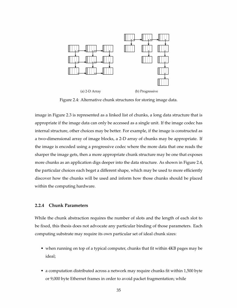
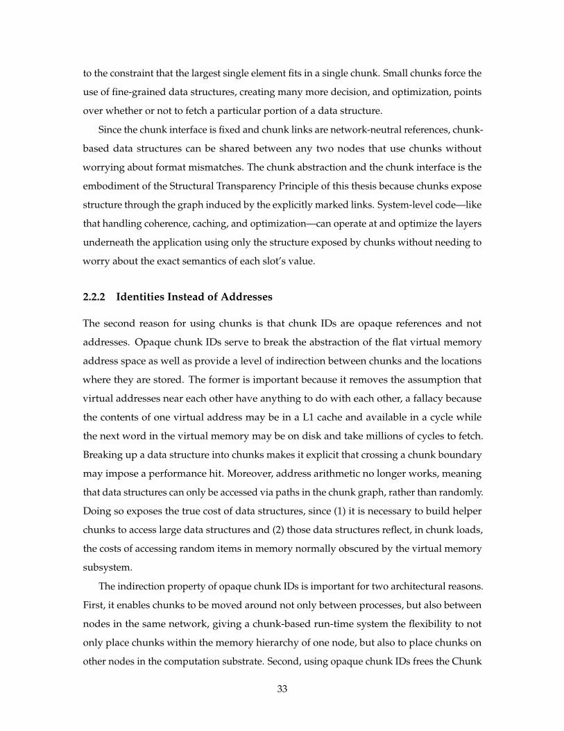
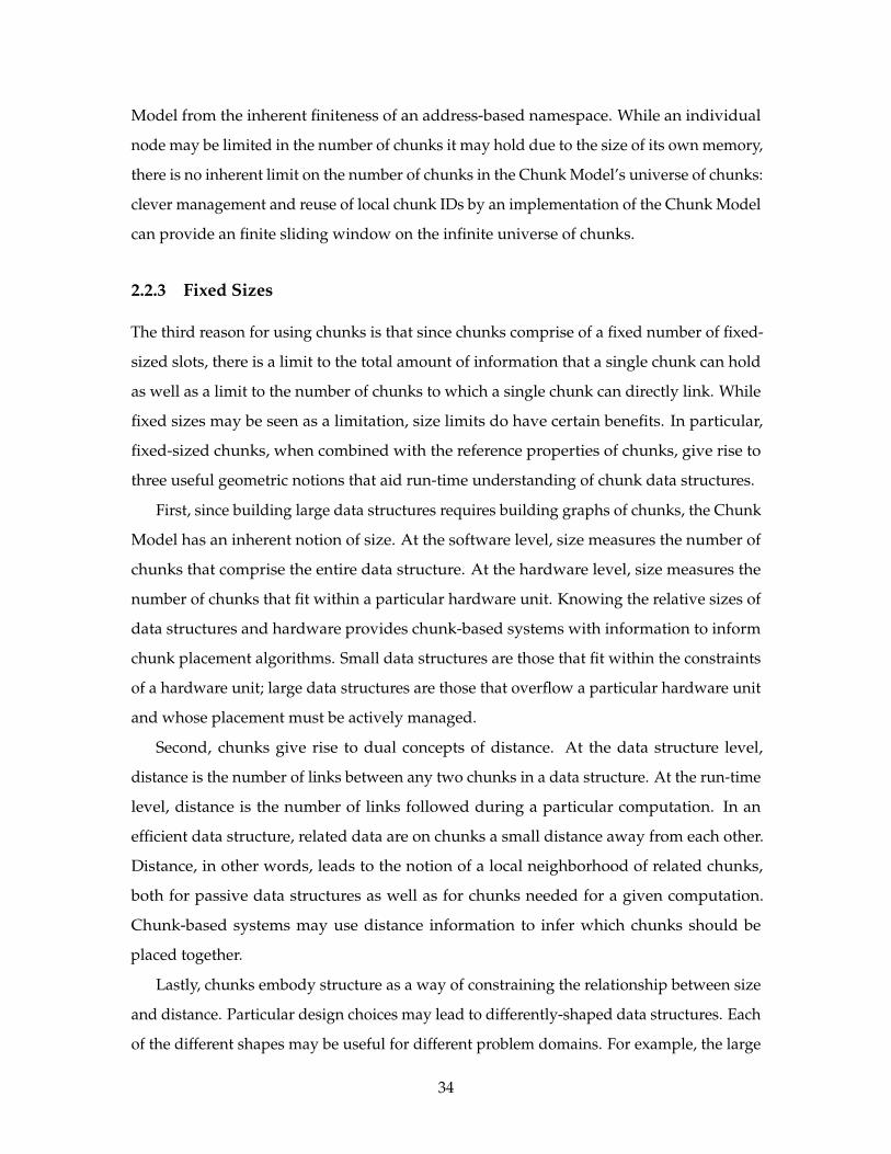
(a) 2-D Array (b) Progressive

Figure 2.4: Alternative chunk structures for storing image data.

image in Figure 2.3 is represented as a linked list of chunks, a long data structure that is

appropriate if the image data can only be accessed as a single unit. If the image codec has

internal structure, other choices may be better. For example, if the image is constructed as

a two-dimensional array of image blocks, a 2-D array of chunks may be appropriate. If

the image is encoded using a progressive codec where the more data that one reads the

sharper the image gets, then a more appropriate chunk structure may be one that exposes

more chunks as an application digs deeper into the data structure. As shown in Figure 2.4,

the particular choices each beget a different shape, which may be used to more efficiently

discover how the chunks will be used and inform how those chunks should be placed

within the computing hardware.

2.2.4 Chunk Parameters

While the chunk abstraction requires the number of slots and the length of each slot to

be fixed, this thesis does not advocate any particular binding of those parameters. Each

computing substrate may require its own particular set of ideal chunk sizes:

• when running on top of a typical computer, chunks that fit within 4KB pages may be

ideal;

• a computation distributed across a network may require chunks fit within 1,500 byte

or 9,000 byte Ethernet frames in order to avoid packet fragmentation; while

35

• a massively multi-core machine may work best when a chunk fits in a small number

of chip-network flits.

All that matters for the abstraction to work is that a particular choice is made, that the

choice enable each chunk to have at least a small number of slots1 and that the same choice

is used throughout the computing substrate.

2.3 Example Chunk Structures

The Chunk Model enables the construction of application-specific data structures using a

generic foundation; the only problem is figuring out how to represent application-specific

data in chunks in a way that adheres to the Structural Navigability Principle. To help

ground how chunks may be used consider two disparate problems: video streaming and

general computing.

2.3.1 ChunkStream: Chunks for Video

Video is an ideal candidate for structured computing systems since video data is inherently

structured, yet must be flattened into byte-oriented container formats for storage and

transfer in traditional computing systems. Video container formats serve as application-

specific structuring mechanisms in that they enable a video player to search within the

byte-oriented video file or stream and pick out the underlying video codec data that the

player needs to decode and display the video. Each container format is optimized for a

particular use case and, as such, may offer only certain features. Some, like MPEG-TS [1],

only allow forward playback, while others like MPEG-PS [1], AVI [69], and MKV [67] also

allow video players to seek to particular locations, while others, like the professional-level

MXF container format [3] are optimized for frame-accurate video editing.

ChunkStream’s video representation is guided by the observation that video playback

consists of finding frame data in the order it needs to be decoded and displayed. If the

representation of each video stream were a linked list of still frames, playback would be the

act of running down the linked list.

1The lower bound of the number of chunks per slot is two, making chunks akin to LISP cons cells, but wefind that a lower bound closer to 8 is much more useful since it gives applications more room to distinguishbetween slots for their own purposes.

36

IndexTree

Backbone

LaneMarkers

FrameData

Lane #0(HD)

Lane #1(low-bandwidth)

Frame #1 Frame #2 Frame #3 Frame #4

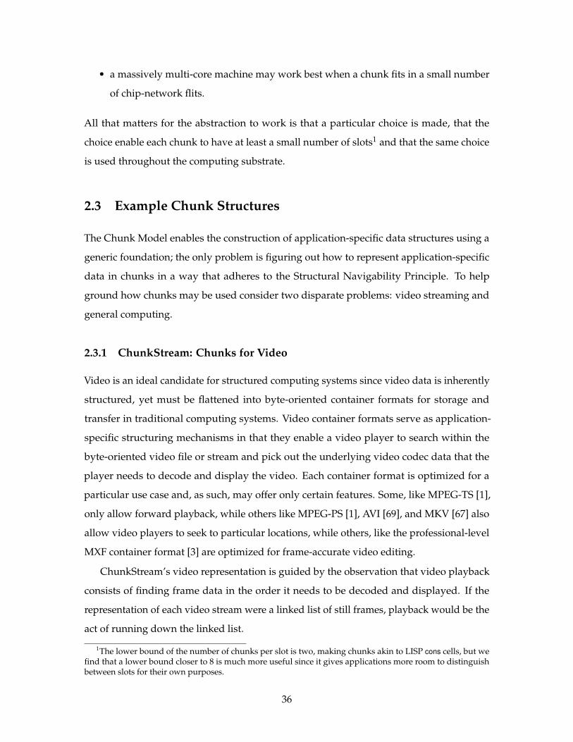
Figure 2.5: Chunk-based video stream representation used by ChunkStream. LaneMarkerchunks represent logical frames and point to “lanes” composed of FrameData chunks. Eachlane represents the frame in different formats, e.g. using HD or low-bandwidth encodings.Links to StreamDescription chunks and unused slots at the end of chunks are not shown.

With those observations in mind, ChunkStream represents video streams with four

types of chunks, as illustrated in Figure 2.5. The underlying stream is represented as a

doubly-linked list of “backbone” chunks that connect representations of individual frames.

The backbone is doubly-linked to allow forwards and backwards movement within the

stream. For each frame in the video clip, the backbone links to a “LaneMarker” chunk that

represents the frame.

The LaneMarker chunk serves two purposes. First, it links to metadata about its frame,

such as frame number or video time code. Second, the LaneMarker links to “lanes” of

video. A lane is a video sub-stream of a certain bandwidth and quality, similar to segment

variants in HTTP Live Streaming [81]. A typical LaneMarker might have three lanes: one

high-quality high-definition (HD) lane for powerful devices, a low-quality lane suitable for

playback over low-bandwidth connections on small devices, and a thumbnail lane that acts

as a stand-in for frames in static situations, like a timeline. ChunkStream requires that each

lane be semantically equivalent (even if the decoded pictures are different) so that the client

may choose the lane it deems appropriate based on its resources.

Each lane takes up two slots in the LaneMarker chunk. One of these lane slots contains

a link to a StreamDescription chunk. The StreamDescription chunk contains a description

37

1 def play(tree_root , frame_num):23 # Search through the IndexTree:4 backbone = indextree_find_frame(tree_root, frame_num)56 while playing:7 # Dereference links from the backbone down to frame data:8 lm_chunk = get_lane_marker(backbone, frame_num)9 lane_num = choose_lane(lm_chunk)

10 frame_data = read_lane(lm_chunk, lane_num)11 # Decode the data we have12 deocde_frame(frame_data)1314 # Advance to next frame in backbone:15 (backbone, frame_num) = get_next(backbone, frame_num)

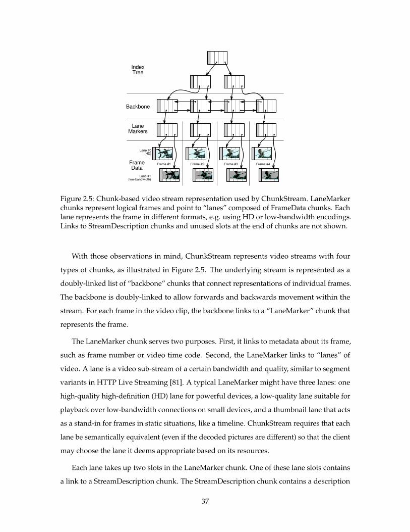
Listing 2.1: Client-side playback algorithm for ChunkStream.

of the lane, including the codec, stream profile information, picture size parameters, stream

bit rate, and any additional flags that are needed to decode the lane. Lanes are not explic-

itly marked with identifiers like “HD” or “low-bandwidth”. Instead, clients derive this

information from the parameters of the stream: a resource-constrained device may bypass

a 1920x1080 “High Profile” stream in favor of a 480x270 “Baseline” profile stream while

a well-connected desktop computer may make the opposite choice. As an optimization,

ChunkStream makes use of the fact that in most video clips, the parameters of stream do not

change over the life of the stream, allowing ChunkStream to use a single StreamDescription

chunk for each lane and point to that single chunk from each LaneMarker.

The other slot of the lane points to a FrameData chunk that contains the underlying

encoded video data densely packed into slots. If the frame data does not fit within a single

chunk, the FrameData chunk may link to other FrameData chunks.

Finally, in order to enable efficient, O(log n) random frame seeking (where n is the

total number of frames), the top of the ChunkStream data structure contains a search tree,

consisting of IndexTree chunks, that maps playback frame numbers to backbone chunks.

Video Playback

Listing 2.1 shows the algorithm clients use to play a video clip in ChunkStream. A client

first searches through the IndexTree for the backbone chunk containing the first frame to

play. From the backbone chunk, the client follows a link to the LaneMarker for the first

frame, downloads any necessary StreamDescription chunks, and examines their contents to

determine which lane to play. Finally, the client de-references the link for its chosen lane to

38

fetch the actual frame data and decodes the frame. To play the next frame, the client steps

to the next element in the backbone and repeats the process of finding frame data from the

backbone chunk.

Advantages of the Chunk Model

An advantage of exposing chunks directly to the client is that new behaviors can be im-

plemented without changing the chunk format or the protocols for transferring chunks

between the video player and the video server. For example, the basic playback algorithm

of Listing 2.1 can be extended with additional features by simply altering the order and

number of frames read from the backbone. In particular, a client can support reverse play-

back by stepping backwards through the backbone instead of forwards. Other operations,

like high-speed playback in either direction may be implemented by skipping over frames

in the backbone based on how fast playback should proceed.

It is also possible to implement new server-side behaviors, such as live streaming of

real-time video. Doing so simply requires dynamically adding new frames to the backbone

and lazily updating the IndexTree so that new clients can quickly seek to the end of the

stream.

2.3.2 CVM: Computing with Chunks

While ChunkStream is an example of using chunks for data structures, chunks are also a

useful foundation for computation. One way to use chunks for computation is to make use

of the standard “stored program” computer trick and use chunks as the backing store for

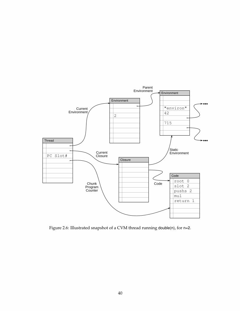
all state—including executable code, program data, and machine state. Figure 2.6 shows

an example computation expressed in chunks for a computing system based on closures

and environments2. We call this the CVM data structure, since it represents a chunk-based

virtual machine.

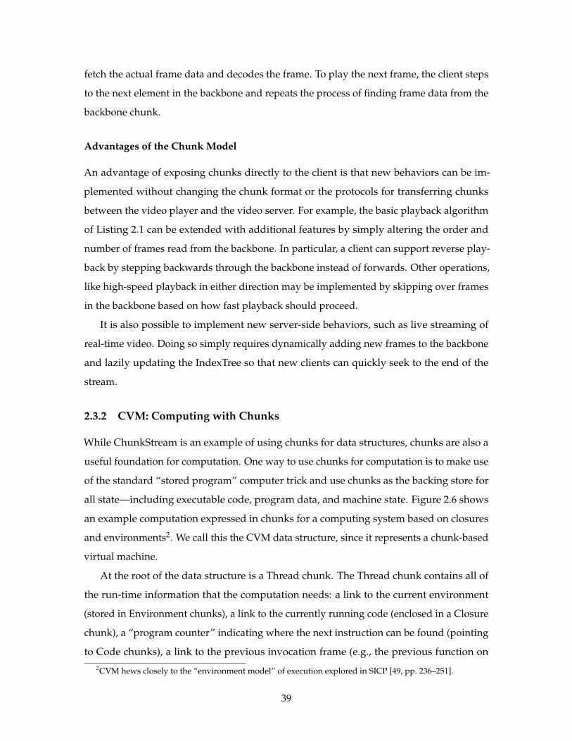
At the root of the data structure is a Thread chunk. The Thread chunk contains all of

the run-time information that the computation needs: a link to the current environment

(stored in Environment chunks), a link to the currently running code (enclosed in a Closure

chunk), a “program counter” indicating where the next instruction can be found (pointing

to Code chunks), a link to the previous invocation frame (e.g., the previous function on2CVM hews closely to the “environment model” of execution explored in SICP [49, pp. 236–251].

39

Code

pushs 2

root 0

slot 2

mul

return 1

Environment

2

Environment

"environ"

42

715

Thread

PC Slot#

CurrentEnvironment

ChunkProgramCounter

ParentEnvironment

StaticEnvironment

Code

CurrentClosure

•••

•••

Closure

Figure 2.6: Illustrated snapshot of a CVM thread running double(n), for n=2.

40

the stack), as well as slots for temporary storage (e.g., machine registers or machine stack).

Each Environment chunk represents a scoped environment for computations; each slot in

the Environment chunks represents a program variable. The Closure chunk points to both

the closure’s static environment as well as its code.

A machine using the CVM data structure starts a cycle of computation by de-referencing

program counter chunk and then reading the instruction at the program counter slot. The

instruction may read or write temporary values in the Thread chunk or modify chunks

linked to by the Thread chunk. After the instruction executes, the program counter is

updated to point the next instruction, which may be in another chunk as in the case of

branches or jumps.

Migration with CVM

A consequence of the Chunk Model only allowing chunks to reference other chunks through

links is that CVM computations can only access chunks transitively linked from the root

Thread chunk. This constraint forces the CVM data structures to be self-contained: each

Thread chunk necessarily points to all of the code and data that the computation uses. A

consequence of this property is that it is easy to move threads of computations between

nodes running a CVM computation.

To migrate computation between CVM instances, the source VM need only send the root

Thread chunk to the destination VM. As the destination VM reads links from the chunk, it

will request more chunks from the source VM until it has copied enough chunks to make

progress on the computation.

In many ways, the CVM migration strategy is similar to standard on-demand paging

schemes. However, it is possible to exploit two properties of the CVM chunk representation

to speed up migration. First, the fine-grained nature of the CVM data structure allows

the migration of only small portions of running programs, such as an individual function,

individual data objects, or even just the code and objects from a particular execution path,

rather than an entire binary and its resident memory. Second, it is possible to exploit locality

exposed by explicit links during the migration process and send all chunks within some

link radius of the Thread chunk all at once, under the assumption that chunks close to a

computation’s Thread chunk are likely to be used by that computation. For example, in

41

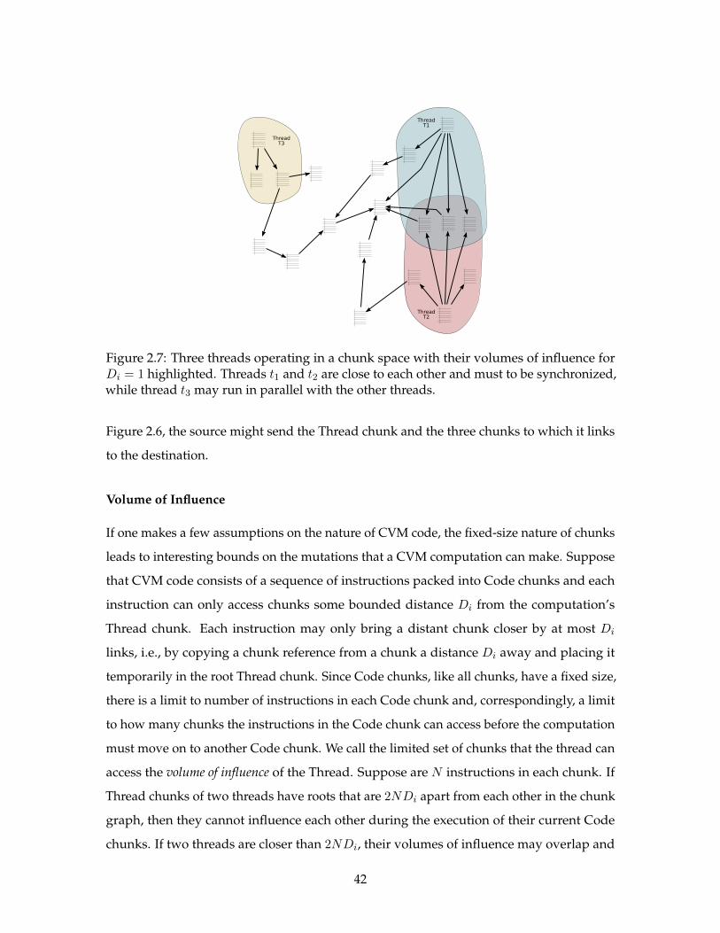
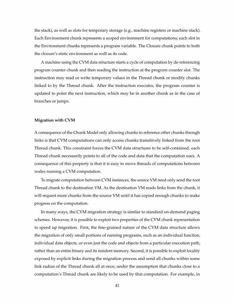
ThreadT1

ThreadT2

ThreadT3

Figure 2.7: Three threads operating in a chunk space with their volumes of influence forDi = 1 highlighted. Threads t1 and t2 are close to each other and must to be synchronized,while thread t3 may run in parallel with the other threads.

Figure 2.6, the source might send the Thread chunk and the three chunks to which it links

to the destination.

Volume of Influence

If one makes a few assumptions on the nature of CVM code, the fixed-size nature of chunks

leads to interesting bounds on the mutations that a CVM computation can make. Suppose

that CVM code consists of a sequence of instructions packed into Code chunks and each

instruction can only access chunks some bounded distance Di from the computation’s

Thread chunk. Each instruction may only bring a distant chunk closer by at most Di

links, i.e., by copying a chunk reference from a chunk a distance Di away and placing it

temporarily in the root Thread chunk. Since Code chunks, like all chunks, have a fixed size,

there is a limit to number of instructions in each Code chunk and, correspondingly, a limit

to how many chunks the instructions in the Code chunk can access before the computation

must move on to another Code chunk. We call the limited set of chunks that the thread can

access the volume of influence of the Thread. Suppose are N instructions in each chunk. If

Thread chunks of two threads have roots that are 2NDi apart from each other in the chunk

graph, then they cannot influence each other during the execution of their current Code

chunks. If two threads are closer than 2NDi, their volumes of influence may overlap and

42

may need to be considered together by the hardware management and chunk placement

layer.

For example, consider Figure 2.7, in which three threads execute in a chunk space.

Threads t1 and t3 are far away from each other in the space and may be able to run

concurrently without competing for resources like memory bandwidth. In contrast, threads

t1 and t2 have overlapping volumes of influence and must time-share memory bandwidth

and synchronize access to their shared chunks. The substrate’s run-time system may be

able to use this information to, e.g., place t1 and t2 on the same processor core so they can

share chunks using higher-performance local communication primitives, while placing t3

on a separate core that runs in near-isolation with no synchronization overhead with other

threads.

43

Chapter 3

The Chunk Platform

The previous chapter outlined the Chunk Model, both as a data model and as a computation

model. This chapter outlines the Chunk Platform, an implementation of the Chunk Model.

The Chunk Platform serves as a vehicle for evaluating the hypothesis that preserving

structure with chunks at machine abstraction layer makes it easier to provide system

support for modern computing substrates.

There are many possible implementations of the Chunk Model, each of which makes

different implementation choices emphasizing particular engineering trade-offs. Since our

focus is on validating the Chunk Model, the design of the Chunk Platform is optimized

toward experimenting with and debugging applications running on top of the model,

and prototyping the systems layer that provides services like persistence, consistency,

and garbage collection of chunks. The implementation of the Chunk Platform focuses

on simplicity rather than raw performance. In doing so, the Chunk Platform provides a

foundation focused on maximizing the abilities of the Chunk Model while minimizing the

pain points, both in implementation and overheads, of using the Chunk Model.

3.1 Chunk Platform Overview

Recall that the Chunk Model targets modern computing substrates like general-purpose

GPUs, massively multi-core processors, and elastic cloud computing systems. While

modern computing substrates vary at the low level, they share two common properties:

45

ChunkRuntime

ChunkRuntime

ChunkRuntime

ChunkRuntime

ChunkRuntime

ChunkRuntime

App 1 App 1

App 2App 1

App 3

App 4

App 4

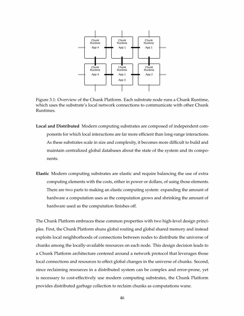
Figure 3.1: Overview of the Chunk Platform. Each substrate node runs a Chunk Runtime,which uses the substrate’s local network connections to communicate with other ChunkRuntimes.

Local and Distributed Modern computing substrates are composed of independent com-

ponents for which local interactions are far more efficient than long-range interactions.

As these substrates scale in size and complexity, it becomes more difficult to build and

maintain centralized global databases about the state of the system and its compo-

nents.

Elastic Modern computing substrates are elastic and require balancing the use of extra

computing elements with the costs, either in power or dollars, of using those elements.

There are two parts to making an elastic computing system: expanding the amount of

hardware a computation uses as the computation grows and shrinking the amount of

hardware used as the computation finishes off.

The Chunk Platform embraces these common properties with two high-level design princi-

ples. First, the Chunk Platform shuns global routing and global shared memory and instead

exploits local neighborhoods of connections between nodes to distribute the universe of

chunks among the locally-available resources on each node. This design decision leads to

a Chunk Platform architecture centered around a network protocol that leverages those

local connections and resources to effect global changes in the universe of chunks. Second,

since reclaiming resources in a distributed system can be complex and error-prone, yet

is necessary to cost-effectively use modern computing substrates, the Chunk Platform

provides distributed garbage collection to reclaim chunks as computations wane.

46

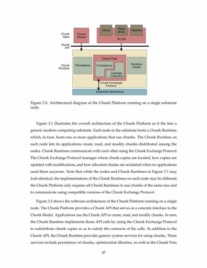
ChunkStream

SCVM

JSLitePhotoBoss

Tasklets

ChunkAPI

ChunkApps

Substrate Networking

ChunkRuntime

RuntimeHooks

GarbageCollection

ConsistencyPersistence

Chunk ExchangeProtocol

Chunk Peer

Figure 3.2: Architectural diagram of the Chunk Platform running on a single substratenode.

Figure 3.1 illustrates the overall architecture of the Chunk Platform as it fits into a

generic modern computing substrate. Each node in the substrate hosts a Chunk Runtime,

which, in turn, hosts one or more applications that use chunks. The Chunk Runtime on

each node lets its applications create, read, and modify chunks distributed among the

nodes. Chunk Runtimes communicate with each other using the Chunk Exchange Protocol.

The Chunk Exchange Protocol manages where chunk copies are located, how copies are

updated with modifications, and how allocated chunks are reclaimed when no applications

need them anymore. Note that while the nodes and Chunk Runtimes in Figure 3.1 may

look identical, the implementations of the Chunk Runtimes on each node may be different;

the Chunk Platform only requires all Chunk Runtimes to use chunks of the same size and

to communicate using compatible versions of the Chunk Exchange Protocol.

Figure 3.2 shows the software architecture of the Chunk Platform running on a single

node. The Chunk Platform provides a Chunk API that serves as a concrete interface to the

Chunk Model. Applications use the Chunk API to create, read, and modify chunks. In turn,

the Chunk Runtime implements those API calls by using the Chunk Exchange Protocol

to redistribute chunk copies so as to satisfy the contracts of the calls. In addition to the

Chunk API, the Chunk Runtime provides generic system services for using chunks. These

services include persistence of chunks, optimization libraries, as well as the Chunk Peer,

47

which handles the Chunk Exchange Protocol. The Chunk Runtime is implemented on top

of a substrate-specific networking layer, e.g., a layer using WebSockets [34] in the cloud, or

on-chip networking instructions in massively multi-core processors.

The rest of this chapter details the particular choices for the Chunk API and the imple-

mentation of the Chunk Runtime that comprise the Chunk Platform.

3.2 The Chunk API and Memory Model

The Chunk API is the application-level expression of the Chunk Model: it provides a

window into the shared universe of chunks and provides mechanisms for manipulating

the chunk graph. The particular Chunk API we chose for the Chunk Runtime balances

the needs of applications—providing standard mechanisms to create, modify, and find

chunks—with the needs of the Chunk Platform—namely knowing when applications are

actively using chunks or actively modifying chunks, in addition to determining when

chunks are no longer needed by applications. As shown in Table 3.1, the API is divided into

four groups of functions: functions to create chunks, functions to read chunks, functions to

modify chunks, and system-level functions used internally within the Chunk Runtime to

manage chunk references across the Chunk Platform’s network of nodes.

3.2.1 API Usage

Chunks are created in two steps. First, applications call new_chunk() to create an nameless,

ephemeral chunk. To insert the chunk into the Chunk Platform, the application calls

insert(chunk), which names the chunk with a chunk ID and persists it within local storage of

the Chunk Runtime. Chunk IDs form the core linking abstraction for the Chunk Platform;

once a chunk has been assigned an ID, that chunk can be used as a link target of other

chunks as well as a parameter to the Chunk API. If an application attempts to de-reference

an invalid chunk ID, the Chunk Runtime will raise an exception, much like de-referencing

an invalid address may cause a virtual memory system to cause a general protection fault.

For example, to create the data structure in Figure 2.2, we first call new_chunk() to create

the image chunk. After filling the chunk with image data, we call insert() to persist the

chunk to the store; insert() returns an identifier (#73) to use to refer to the chunk. Next, we

call new_chunk() a second time to create the text chunk. After filling the first seven slots with

48

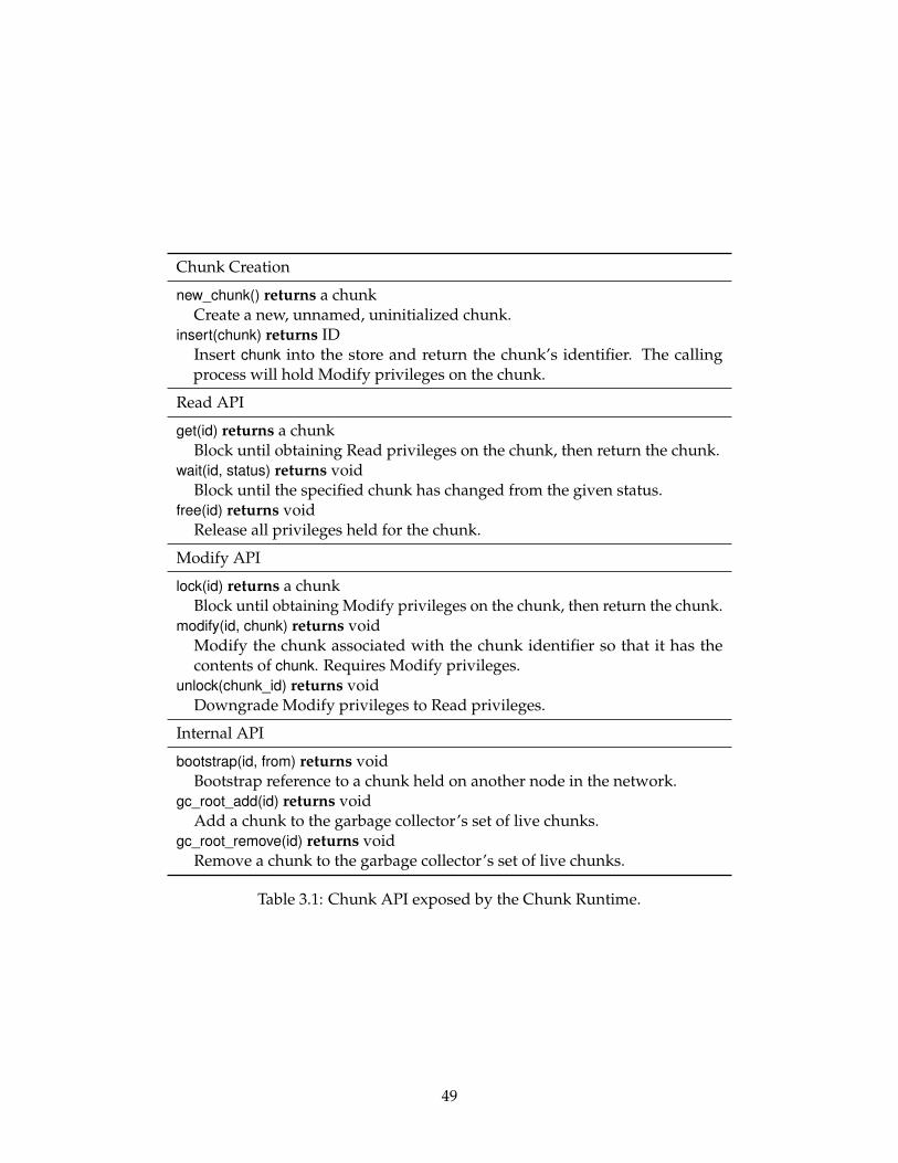
Chunk Creation

new_chunk() returns a chunkCreate a new, unnamed, uninitialized chunk.

insert(chunk) returns IDInsert chunk into the store and return the chunk’s identifier. The callingprocess will hold Modify privileges on the chunk.

Read API

get(id) returns a chunkBlock until obtaining Read privileges on the chunk, then return the chunk.

wait(id, status) returns voidBlock until the specified chunk has changed from the given status.

free(id) returns voidRelease all privileges held for the chunk.

Modify API

lock(id) returns a chunkBlock until obtaining Modify privileges on the chunk, then return the chunk.

modify(id, chunk) returns voidModify the chunk associated with the chunk identifier so that it has thecontents of chunk. Requires Modify privileges.

unlock(chunk_id) returns voidDowngrade Modify privileges to Read privileges.

Internal API

bootstrap(id, from) returns voidBootstrap reference to a chunk held on another node in the network.

gc_root_add(id) returns voidAdd a chunk to the garbage collector’s set of live chunks.

gc_root_remove(id) returns voidRemove a chunk to the garbage collector’s set of live chunks.

Table 3.1: Chunk API exposed by the Chunk Runtime.

49

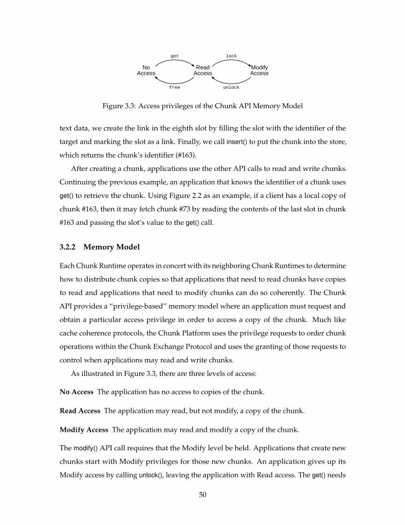
NoAccess

ReadAccess

ModifyAccess

get lock

free unlock

Figure 3.3: Access privileges of the Chunk API Memory Model

text data, we create the link in the eighth slot by filling the slot with the identifier of the

target and marking the slot as a link. Finally, we call insert() to put the chunk into the store,

which returns the chunk’s identifier (#163).

After creating a chunk, applications use the other API calls to read and write chunks.

Continuing the previous example, an application that knows the identifier of a chunk uses

get() to retrieve the chunk. Using Figure 2.2 as an example, if a client has a local copy of

chunk #163, then it may fetch chunk #73 by reading the contents of the last slot in chunk

#163 and passing the slot’s value to the get() call.

3.2.2 Memory Model

Each Chunk Runtime operates in concert with its neighboring Chunk Runtimes to determine

how to distribute chunk copies so that applications that need to read chunks have copies

to read and applications that need to modify chunks can do so coherently. The Chunk

API provides a “privilege-based” memory model where an application must request and

obtain a particular access privilege in order to access a copy of the chunk. Much like

cache coherence protocols, the Chunk Platform uses the privilege requests to order chunk

operations within the Chunk Exchange Protocol and uses the granting of those requests to

control when applications may read and write chunks.

As illustrated in Figure 3.3, there are three levels of access:

No Access The application has no access to copies of the chunk.

Read Access The application may read, but not modify, a copy of the chunk.

Modify Access The application may read and modify a copy of the chunk.

The modify() API call requires that the Modify level be held. Applications that create new

chunks start with Modify privileges for those new chunks. An application gives up its

Modify access by calling unlock(), leaving the application with Read access. The get() needs

50

Read access in order to complete. The get() API call will block until Read level access is

available, e.g., when no other local process or Chunk Peer has Modify access to the chunk.

When an application is done using a copy of a chunk, it calls free() to give up all Read or

Modify privileges on the chunk.

The Chunk API exposes a privilege-based memory abstraction since such an abstraction

can be used to implement any memory consistency model depending on which operations

block, which operations are asynchronous, and which operations are allowed to be rolled

back [14]. The Chunk Runtime implements the Chunk API using a blocking, sequential

consistency memory model [61]. We chose to implement a sequential consistency model

because (1) programmers find sequential consistency, along with its close relative, pro-

cessor consistency, the easiest memory models to program for and (2) sequential- and

processor-consistent memory models still perform relatively well against harder to use

relaxed memory models [6, 50].

3.3 Chunk Runtime

The Chunk Runtime provides an implementation of the Chunk API as well as a variety of

system services useful to applications using chunks.

3.3.1 Persistence

One portion of the Chunk Runtime is the Chunk Store. The Chunk Store provides a

backing store for chunks in use by the Chunk Runtime. The Chunk Runtime provides two

implementations of the backing store. The first guarantees durability of chunks by storing

them on a file system. The other trades off durability for speed by “storing” chunks in the

local memory of the host. An individual node may choose which persistence layer to run

when it boots its local Chunk Runtime.

3.3.2 Runtime Hooks

The Chunk Runtime provides hooks to profile applications using the Chunk API. The

hooks provide a small API that allows an optimization plug-in to observe what chunks

are requested by applications as well as what network and coherence events the applica-

51

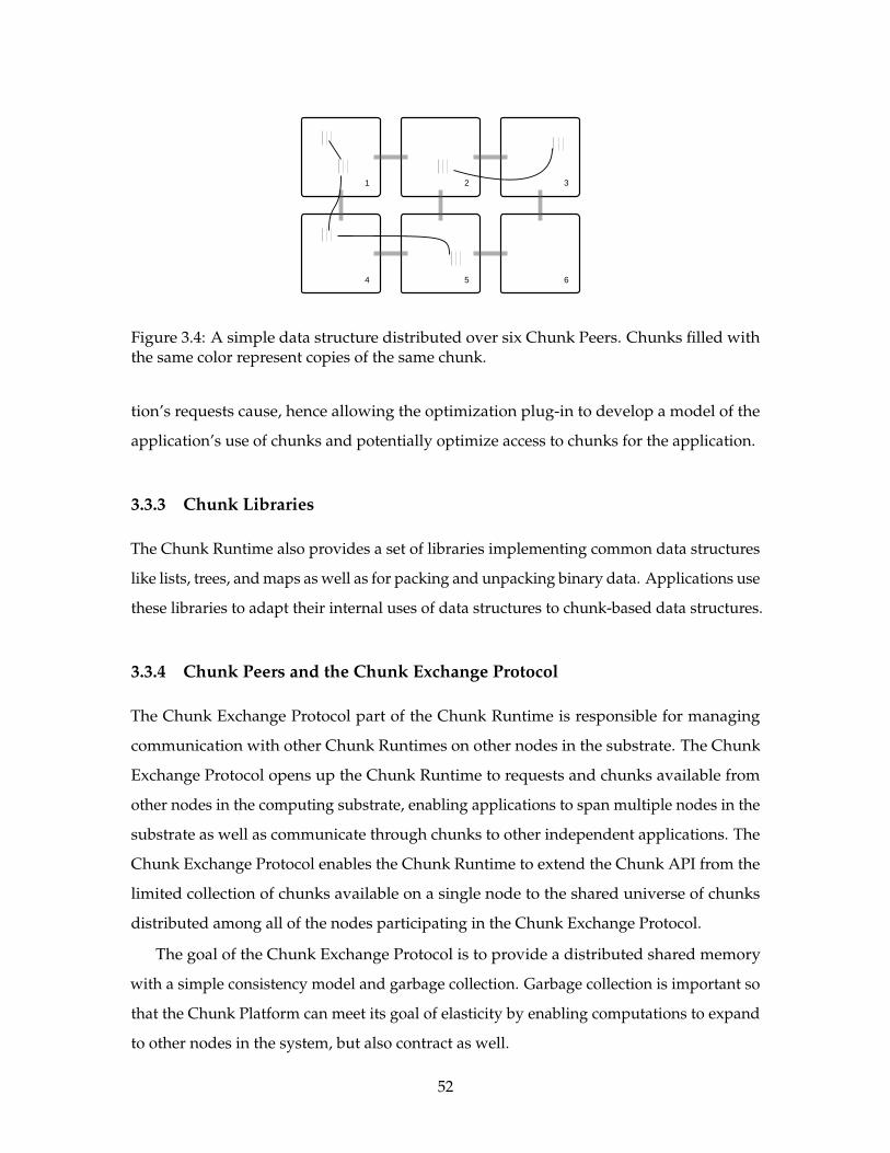
1

4

2 3

5 6

Figure 3.4: A simple data structure distributed over six Chunk Peers. Chunks filled withthe same color represent copies of the same chunk.

tion’s requests cause, hence allowing the optimization plug-in to develop a model of the

application’s use of chunks and potentially optimize access to chunks for the application.

3.3.3 Chunk Libraries

The Chunk Runtime also provides a set of libraries implementing common data structures

like lists, trees, and maps as well as for packing and unpacking binary data. Applications use

these libraries to adapt their internal uses of data structures to chunk-based data structures.

3.3.4 Chunk Peers and the Chunk Exchange Protocol

The Chunk Exchange Protocol part of the Chunk Runtime is responsible for managing

communication with other Chunk Runtimes on other nodes in the substrate. The Chunk

Exchange Protocol opens up the Chunk Runtime to requests and chunks available from

other nodes in the computing substrate, enabling applications to span multiple nodes in the

substrate as well as communicate through chunks to other independent applications. The

Chunk Exchange Protocol enables the Chunk Runtime to extend the Chunk API from the

limited collection of chunks available on a single node to the shared universe of chunks

distributed among all of the nodes participating in the Chunk Exchange Protocol.

The goal of the Chunk Exchange Protocol is to provide a distributed shared memory

with a simple consistency model and garbage collection. Garbage collection is important so

that the Chunk Platform can meet its goal of elasticity by enabling computations to expand

to other nodes in the system, but also contract as well.

52

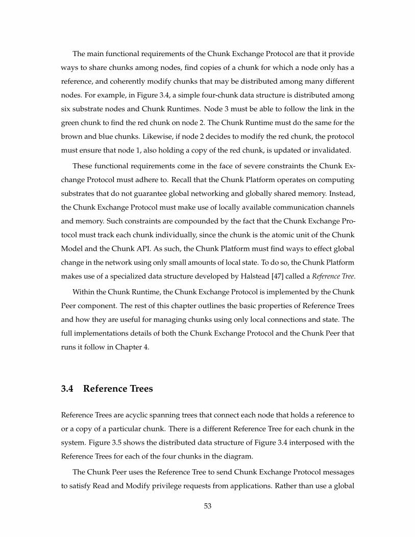
The main functional requirements of the Chunk Exchange Protocol are that it provide

ways to share chunks among nodes, find copies of a chunk for which a node only has a

reference, and coherently modify chunks that may be distributed among many different

nodes. For example, in Figure 3.4, a simple four-chunk data structure is distributed among

six substrate nodes and Chunk Runtimes. Node 3 must be able to follow the link in the

green chunk to find the red chunk on node 2. The Chunk Runtime must do the same for the

brown and blue chunks. Likewise, if node 2 decides to modify the red chunk, the protocol

must ensure that node 1, also holding a copy of the red chunk, is updated or invalidated.

These functional requirements come in the face of severe constraints the Chunk Ex-

change Protocol must adhere to. Recall that the Chunk Platform operates on computing

substrates that do not guarantee global networking and globally shared memory. Instead,

the Chunk Exchange Protocol must make use of locally available communication channels

and memory. Such constraints are compounded by the fact that the Chunk Exchange Pro-

tocol must track each chunk individually, since the chunk is the atomic unit of the Chunk

Model and the Chunk API. As such, the Chunk Platform must find ways to effect global

change in the network using only small amounts of local state. To do so, the Chunk Platform

makes use of a specialized data structure developed by Halstead [47] called a Reference Tree.

Within the Chunk Runtime, the Chunk Exchange Protocol is implemented by the Chunk

Peer component. The rest of this chapter outlines the basic properties of Reference Trees

and how they are useful for managing chunks using only local connections and state. The

full implementations details of both the Chunk Exchange Protocol and the Chunk Peer that

runs it follow in Chapter 4.

3.4 Reference Trees

Reference Trees are acyclic spanning trees that connect each node that holds a reference to

or a copy of a particular chunk. There is a different Reference Tree for each chunk in the

system. Figure 3.5 shows the distributed data structure of Figure 3.4 interposed with the

Reference Trees for each of the four chunks in the diagram.

The Chunk Peer uses the Reference Tree to send Chunk Exchange Protocol messages

to satisfy Read and Modify privilege requests from applications. Rather than use a global

53

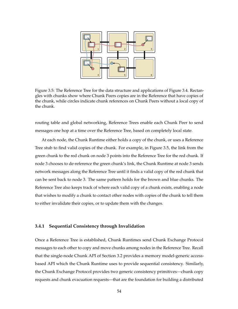
1

4

2 3

5 6

Figure 3.5: The Reference Tree for the data structure and applications of Figure 3.4. Rectan-gles with chunks show where Chunk Peers copies are in the Reference that have copies ofthe chunk, while circles indicate chunk references on Chunk Peers without a local copy ofthe chunk.

routing table and global networking, Reference Trees enable each Chunk Peer to send

messages one hop at a time over the Reference Tree, based on completely local state.

At each node, the Chunk Runtime either holds a copy of the chunk, or uses a Reference

Tree stub to find valid copies of the chunk. For example, in Figure 3.5, the link from the

green chunk to the red chunk on node 3 points into the Reference Tree for the red chunk. If

node 3 chooses to de-reference the green chunk’s link, the Chunk Runtime at node 3 sends

network messages along the Reference Tree until it finds a valid copy of the red chunk that

can be sent back to node 3. The same pattern holds for the brown and blue chunks. The

Reference Tree also keeps track of where each valid copy of a chunk exists, enabling a node

that wishes to modify a chunk to contact other nodes with copies of the chunk to tell them

to either invalidate their copies, or to update them with the changes.

3.4.1 Sequential Consistency through Invalidation

Once a Reference Tree is established, Chunk Runtimes send Chunk Exchange Protocol

messages to each other to copy and move chunks among nodes in the Reference Tree. Recall

that the single-node Chunk API of Section 3.2 provides a memory model-generic access-

based API which the Chunk Runtime uses to provide sequential consistency. Similarly,

the Chunk Exchange Protocol provides two generic consistency primitives—chunk copy

requests and chunk evacuation requests—that are the foundation for building a distributed

54

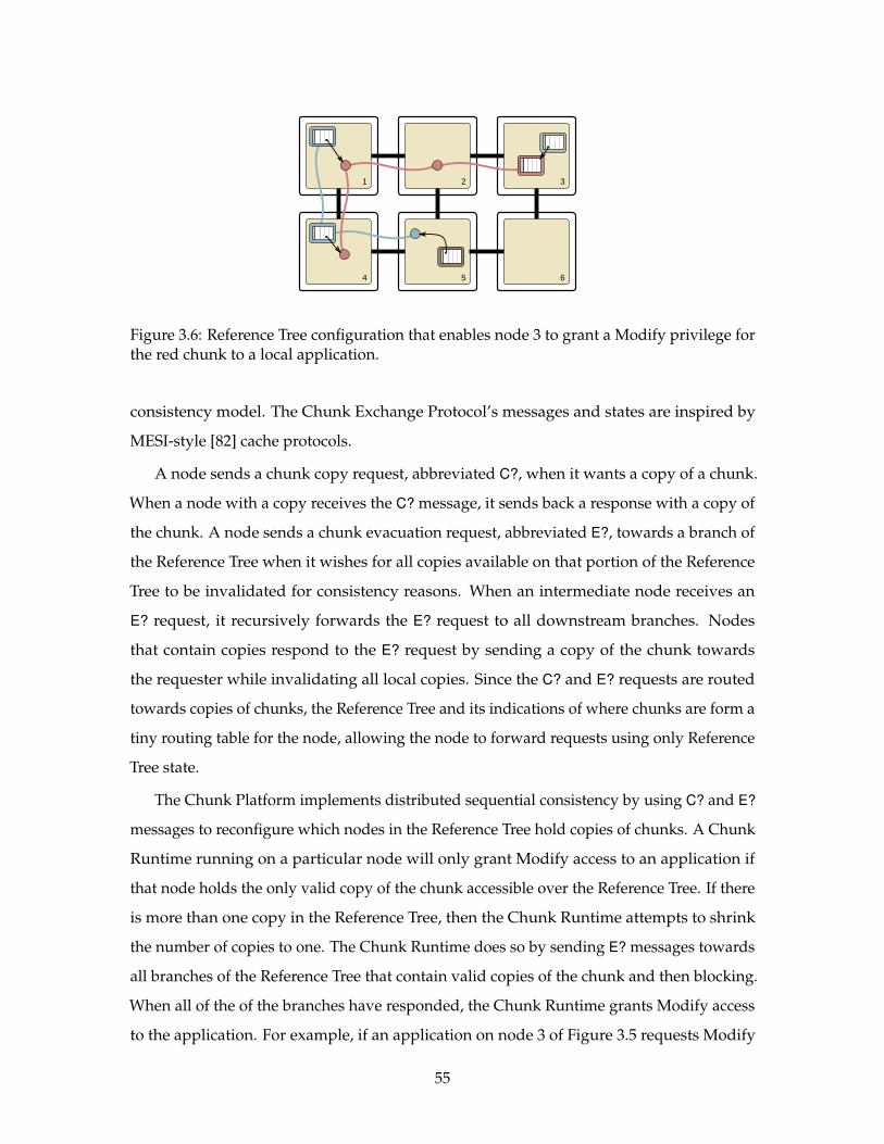
1

4

2 3

5 6

Figure 3.6: Reference Tree configuration that enables node 3 to grant a Modify privilege forthe red chunk to a local application.

consistency model. The Chunk Exchange Protocol’s messages and states are inspired by

MESI-style [82] cache protocols.

A node sends a chunk copy request, abbreviated C?, when it wants a copy of a chunk.

When a node with a copy receives the C? message, it sends back a response with a copy of

the chunk. A node sends a chunk evacuation request, abbreviated E?, towards a branch of

the Reference Tree when it wishes for all copies available on that portion of the Reference

Tree to be invalidated for consistency reasons. When an intermediate node receives an

E? request, it recursively forwards the E? request to all downstream branches. Nodes

that contain copies respond to the E? request by sending a copy of the chunk towards

the requester while invalidating all local copies. Since the C? and E? requests are routed

towards copies of chunks, the Reference Tree and its indications of where chunks are form a

tiny routing table for the node, allowing the node to forward requests using only Reference

Tree state.

The Chunk Platform implements distributed sequential consistency by using C? and E?

messages to reconfigure which nodes in the Reference Tree hold copies of chunks. A Chunk

Runtime running on a particular node will only grant Modify access to an application if

that node holds the only valid copy of the chunk accessible over the Reference Tree. If there

is more than one copy in the Reference Tree, then the Chunk Runtime attempts to shrink

the number of copies to one. The Chunk Runtime does so by sending E? messages towards

all branches of the Reference Tree that contain valid copies of the chunk and then blocking.

When all of the of the branches have responded, the Chunk Runtime grants Modify access

to the application. For example, if an application on node 3 of Figure 3.5 requests Modify

55

access to the red chunk, the Chunk Peer on node 3 will send an E? message toward node

2 to evacuate copies of the chunk on that branch of the Reference Tree. Node 2 forwards

the E? message to node 1. When node 1’s applications relinquish their access privileges to

the red chunk, node 1 responds to node 2 by giving up its copy of the chunk and sending

it to node 2. Node 2, in turn, responds to node 3, by giving up its copy of the chunk and

sending it to node 3. When node 3 gets a response from node 2, the Reference Tree for the

red chunk will look as illustrated in Figure 3.6. At this point, node 3 knows that it has the

only copy of the chunk and grants the Modify privilege to the application that requested it.

The Read privilege case is easier: the Chunk Runtime sends a C? message towards a

branch of the Reference Tree that contains a copy and blocks until it receives a response.

Since multiple nodes can have Read privileges to the same chunk at the same time, a node

that receives the C? message can respond with a copy of the chunk as long as it hasn’t

granted Modify privileges to the chunk to a local application.

Since requests may be spontaneously generated by the Chunk Exchange layer in re-

sponse to Chunk API calls from local applications, the Chunk Peer must take care to resolve

race conditions so that competing, but conflicting requests, are not granted simultaneously.

Rather than use a global clock or other time-based priority schemes, the Chunk Exchange

Protocol orders requests by request type and then by the ID of the requester. Every Chunk

Peer uses the same ordering so that each Chunk Peer responds to the same set of requests

in the same order, even if they do not receive the requests in the same sequence.

For example, in Figure 3.7, suppose that an application on node 1 and an application on

node 4 both request Modify access to the same chunk. The E? request messages induced

by those requests will necessarily cross each other as they flow through the Reference Tree

towards copies that must be evacuated. When the requests intersect at node 2, node 2’s

node will order the messages based on priority. Since both are E? messages, the request

from the node with the lower requester ID will win out and be serviced first. In the situation

of Figure 3.7b, the E?1 from node 1 will win out. When node 2 services node 1’s higher

priority E? request, node 2 will forward the higher-priority request towards node 3 since

that branch of the Reference Tree contains a chunk copy that needs to be evacuated. At

node 3, the E?1 request becomes the new highest priority request, causing it to forward the

E?1 request towards node 4. When E?1 reaches node 4, it will become the highest priority,

beating out node 4’s own request. As such, node 4 will respond by evacuating its copy of

56

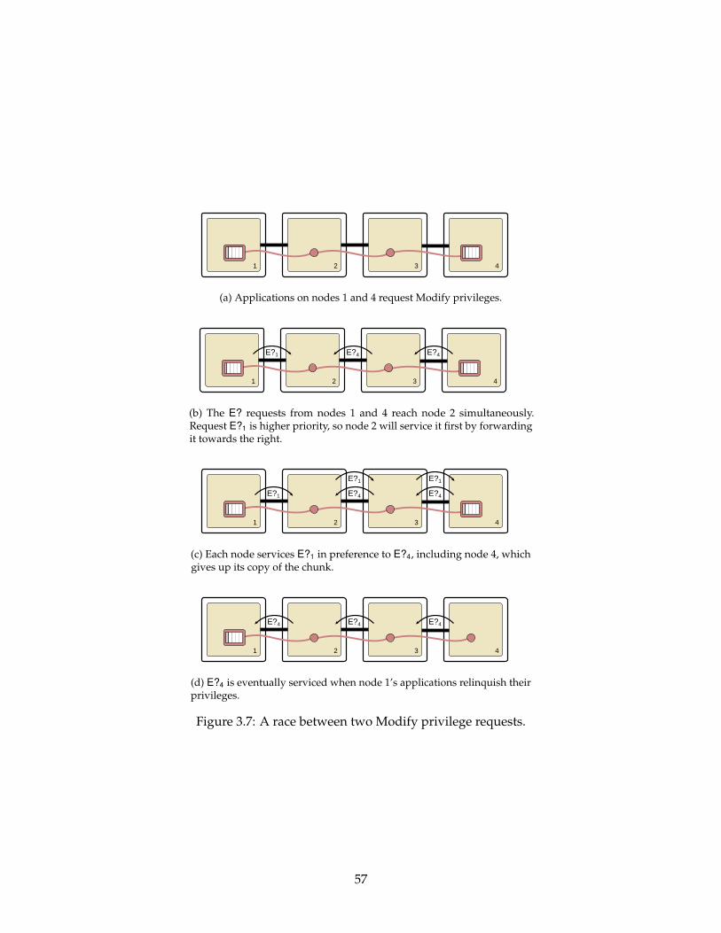
1 2 43

(a) Applications on nodes 1 and 4 request Modify privileges.

1 2 43

E?1 E?4E?4

(b) The E? requests from nodes 1 and 4 reach node 2 simultaneously.Request E?1 is higher priority, so node 2 will service it first by forwardingit towards the right.

1 2 43

E?1

E?1 E?1

E?4E?4

(c) Each node services E?1 in preference to E?4, including node 4, whichgives up its copy of the chunk.

1 2 43

E?4E?4E?4

(d) E?4 is eventually serviced when node 1’s applications relinquish theirprivileges.

Figure 3.7: A race between two Modify privilege requests.

57

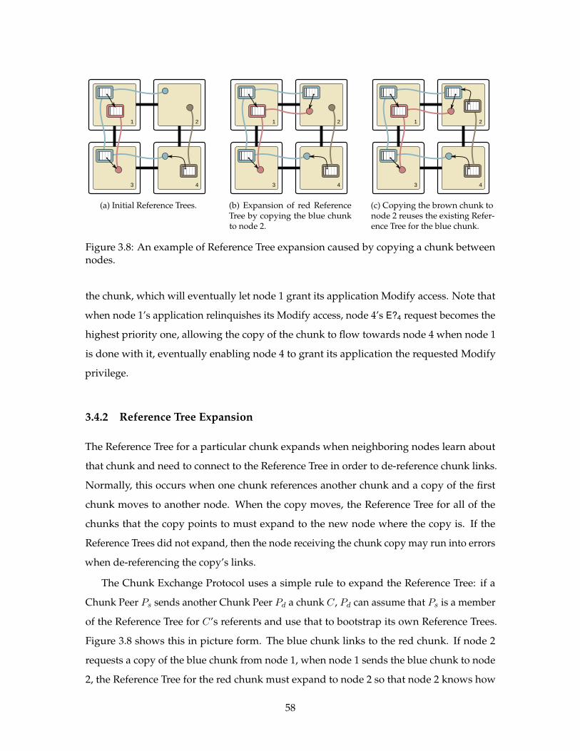
1

3

2

4

(a) Initial Reference Trees.

1

3

2

4

(b) Expansion of red ReferenceTree by copying the blue chunkto node 2.

1

3

2

4

(c) Copying the brown chunk tonode 2 reuses the existing Refer-ence Tree for the blue chunk.

Figure 3.8: An example of Reference Tree expansion caused by copying a chunk betweennodes.

the chunk, which will eventually let node 1 grant its application Modify access. Note that

when node 1’s application relinquishes its Modify access, node 4’s E?4 request becomes the

highest priority one, allowing the copy of the chunk to flow towards node 4 when node 1

is done with it, eventually enabling node 4 to grant its application the requested Modify

privilege.

3.4.2 Reference Tree Expansion

The Reference Tree for a particular chunk expands when neighboring nodes learn about

that chunk and need to connect to the Reference Tree in order to de-reference chunk links.

Normally, this occurs when one chunk references another chunk and a copy of the first

chunk moves to another node. When the copy moves, the Reference Tree for all of the

chunks that the copy points to must expand to the new node where the copy is. If the

Reference Trees did not expand, then the node receiving the chunk copy may run into errors

when de-referencing the copy’s links.

The Chunk Exchange Protocol uses a simple rule to expand the Reference Tree: if a

Chunk Peer Ps sends another Chunk Peer Pd a chunk C, Pd can assume that Ps is a member

of the Reference Tree for C’s referents and use that to bootstrap its own Reference Trees.

Figure 3.8 shows this in picture form. The blue chunk links to the red chunk. If node 2

requests a copy of the blue chunk from node 1, when node 1 sends the blue chunk to node

2, the Reference Tree for the red chunk must expand to node 2 so that node 2 knows how

58

to de-reference all of the links in the chunk. The expansion results in the Reference Tree

configuration of Figure 3.8b.

When the Reference Tree expands to encompass a new link, the Chunk Exchange

Protocol must ensure that no loops are formed to maintain the acyclic property of Reference

Trees. For example, in Figure 3.8, the Reference Tree for the blue chunk already extends

to all of the nodes in the system. If the brown chunk were copied from node 4 to node 2,

the Chunk Exchange Protocol prevents the link from node 4 to node 2 from being used in

the blue chunk’s Reference Tree. However, as shown in Figure 3.8c, rejecting the link will

not break connectivity for the brown chunk’s links, since node 2 is already is a part of the

blue chunk’s Reference Tree, allowing the system to find the chunk through the existing

Reference Tree.

3.4.3 Garbage Collection

The previous section outlined how Reference Trees elastically expand as a computation or

data structure grows to multiple nodes. However, expansion is only half of what is required

for elastic systems—they must also contract to relinquish resources as computations wind

down. The Chunk Platform relies on garbage collection to reclaim the resources allocated

to chunks, using a strategy proposed by Halstead [47]:

1. The Chunk Runtime on each node runs a local garbage collector to determine which

chunks are live for the applications running within that Chunk Runtime.

2. For each dead chunk, if the Chunk Peer has a local copy of the chunk, the Chunk Peer

attempts to evacuate its copy to another node in the Reference Tree.

3. For each dead chunk, if the node is a leaf of the Reference Tree, the node attempts

to leave the Reference Tree. A Chunk Peer may only leave the tree when it does not

break the reference integrity of chunk links, so the attempt to leave the Reference Tree

may fail. If the Chunk Peer successfully leaves the tree, it has the effect of shrinking

the Reference Tree one node at a time towards the center of the Reference Tree.

4. If the Reference Tree for a chunk has shrunk to a single node, delete the chunk when

that node no longer references it.

59

The above garbage collection strategy allows resources to be reclaimed incrementally: extra

chunk copies are reclaimed through step 2, per-node Reference Tree metadata are reclaimed

by step 3, and, finally, the last remnants of the chunk and its Reference Tree are reclaimed in

step 4.

For example, consider the four nodes in Figure 3.9. Suppose that the local garbage

collectors on all four nodes have determined that no applications make use of chunks;

that is, the chunks are dead according to the garbage collector. According to the garbage

collection strategy, only node 4 can leave the tree immediately. Nodes 2 and 3 must stay in

the Reference Tree in order to maintain connectivity of the tree, while node 1 must stay in

the Reference Tree until it evacuates its copy of the chunk.

Suppose that node 4 leaves the Reference Tree. Figure 3.9b illustrates the resulting

configuration of the Reference Tree. After node 4 leaves the Reference Tree, node 3 becomes

eligible for leaving the Reference Tree if, like node 1, it can evacuate its copy of the chunk.

Suppose that node 3 decides to leave the Reference Tree. To do so, it must evacuate its copy

of the chunk. For reasons that will become clear later in this example, the Chunk Exchange

Protocol disallows Chunk Peers from spontaneously sending chunks to another Chunk

Peer. As such, node 3 cannot send its copy of the chunk to node 2. Instead, as shown in

Figure 3.9c, node 3 must ask node 2 to guarantee the chunk, a process which induces node 2

to request a copy of the chunk from node 3. When the guarantee process completes and

node 3 leaves the Reference Tree, the Reference Tree looks like Figure 3.9d.

At this point, nodes 1 and 2 are both leaves of the Reference Tree and can garbage

collect the red chunk if they get rid of their copies. As alluded to before, nodes cannot

spontaneously send copies to another chunk. This is because in a two node situation it

is possible for the two nodes to send chunks to each other while believing that the other

node no longer has a copy, breaking the Reference Tree. The guarantee process prevents

this because guarantees are requests and like any other request in our system, they are

prioritized and ordered. Therefore, if nodes 1 and 2 simultaneously send guarantees to each

other, due to request ordering rules, node 1’s guarantee request will win out and it will be

able to leave the Reference Tree first. This situation is illustrated by Figure 3.9e.

After node 1 leaves the Reference Tree, only node 2 knows about the chunk, as illustrated

in Figure 3.9f. It can delete the chunk whenever it needs to, completing the process of

garbage collecting the chunk and its Reference Tree.

60

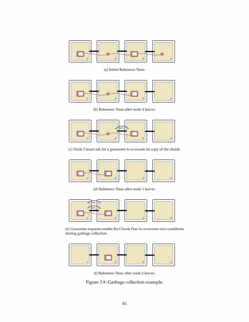
1 2 43

(a) Initial Reference Trees.

1 2 43

(b) Reference Trees after node 4 leaves.

1 2 43

G?3

(c) Node 3 must ask for a guarantee to evacuate its copy of the chunk.

1 2 43

(d) Reference Trees after node 1 leaves.

1 2 43

G?1

G?2

(e) Guarantee requests enable the Chunk Peer to overcome race conditionsduring garbage collection.

1 2 43

(f) Reference Trees after node 2 leaves.

Figure 3.9: Garbage collection example.

61

Garbage collecting chunks essentially amounts to garbage collecting Reference Trees

from nodes that no longer reference those Reference Tree’s chunks. As the example shows,

the key problem in garbage collecting Reference Trees is determining when a node can leave

the Reference Tree without breaking the referential integrity of chunk links—for chunks

referenced locally as well as for chunks referenced by other nodes. This is the subject of the

next chapter.

62

Chapter 4

Taming the Chunk Exchange Protocol

Chapter 3 outlined the architecture of the Chunk Platform and how it uses Chunk Peers,

the Chunk Exchange Protocol, and Reference Trees to share, update, and garbage collect

chunks dispersed among multiple nodes in a computing substrate. This chapter details

the implementation of the Chunk Peer, from the low-level network messages of the Chunk

Exchange Protocol up to the high-level state maintenance loop that runs at the core of each

Chunk Peer component of the Chunk Runtime.

4.1 Chunk Peer

The Chunk Peer component that implements the Chunk Exchange Protocol consists of two

layers. At the lower level is the Channel layer, consisting of Channel Proxies connected

to each networking channel in the computing substrate. At the higher level is the Chunk

Exchange layer, consisting of several components that implement the decision making of

the Chunk Exchange Protocol.

The Chunk Peer is implemented as two layers to enable separation of concerns and to

make the Chunk Peer implementation more modular. The Channel layer manages substrate

networking and maintains the Reference Trees. The Chunk Exchange layer assumes that

the Channel layer provides a working Reference Tree and uses that Reference Tree to (1)

handle the consistent and coherent distribution of chunk copies, (2) mediate requests be-

tween neighboring Chunk Peers and locally running applications, and (3) manage garbage

collection of Reference Trees and chunks.

63

Both the Channel layer and the Chunk Exchange layer are implemented as finite state

machine-like event processing loops that handle incoming events, update local state based

on those events, and then issue responses to those events. Each Reference Tree, and

consequently, each chunk, is tended to by independent instances of the Channel layer and

Chunk Exchange layer components.

Each Channel Proxy in the Channel layer reacts to Chunk Exchange Protocol messages

that come in from its channel. The Channel Proxy parses the network messages to determine

whether the message is a request or a Reference Tree status update. If it is a status update,

the Channel Proxy updates itself to reflect the new status of the branch of the Reference

Tree available over that channel. If the network message is a request, the Channel Proxy

forwards the request to the Chunk Exchange layer. After handling each incoming message,

the Channel layer wakes up the Chunk Exchange layer so it can handle any updated state

or requests.

The Chunk Exchange layer reacts to changes in state at the Channel layer as well as

Chunk API calls from locally running applications. Every time it is woken up, the Chunk

Exchange layer attempts to satisfy the highest-priority request it knows about. If it can

satisfy the request, it does so and deletes the request so it can move on to the next one.

Otherwise the Chunk Exchange layer sends additional requests through the Channel layer

to other Chunk Peers, or if there is nothing more to do, the Chunk Exchange layer suspends

itself until new requests or updates come in.

4.2 Distributed Reference Trees

While the previous chapter discussed Reference Trees as though they are globally consistent

and centrally maintained data structures, in truth Reference Trees are decentralized data

structures whose state is distributed over all Chunk Peers participating in each Reference

Tree.

Each Chunk Peer keeps only enough state about each chunk’s Reference Tree to route

messages and respond to requests for that chunk. In particular, rather than storing, and

needing to maintain, the exact form of each Reference Tree at each node, the Channel layer

of the Chunk Peer instead maintains Channel States for each channel the Chunk Peer has

for each chunk the Chunk Peer references. The Channel State for a channel summarizes

64

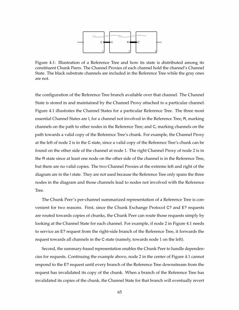
R CC C

1 2 3

Figure 4.1: Illustration of a Reference Tree and how its state is distributed among itsconstituent Chunk Peers. The Channel Proxies of each channel hold the channel’s ChannelState. The black substrate channels are included in the Reference Tree while the gray onesare not.

the configuration of the Reference Tree branch available over that channel. The Channel

State is stored in and maintained by the Channel Proxy attached to a particular channel.

Figure 4.1 illustrates the Channel States for a particular Reference Tree. The three most

essential Channel States are I, for a channel not involved in the Reference Tree; R, marking

channels on the path to other nodes in the Reference Tree; and C, marking channels on the

path towards a valid copy of the Reference Tree’s chunk. For example, the Channel Proxy

at the left of node 2 is in the C state, since a valid copy of the Reference Tree’s chunk can be

found on the other side of the channel at node 1. The right Channel Proxy of node 2 is in

the R state since at least one node on the other side of the channel is in the Reference Tree,

but there are no valid copies. The two Channel Proxies at the extreme left and right of the

diagram are in the I state. They are not used because the Reference Tree only spans the three

nodes in the diagram and those channels lead to nodes not involved with the Reference

Tree.

The Chunk Peer’s per-channel summarized representation of a Reference Tree is con-

venient for two reasons. First, since the Chunk Exchange Protocol C? and E? requests

are routed towards copies of chunks, the Chunk Peer can route those requests simply by

looking at the Channel State for each channel. For example, if node 2 in Figure 4.1 needs

to service an E? request from the right-side branch of the Reference Tree, it forwards the

request towards all channels in the C state (namely, towards node 1 on the left).

Second, the summary-based representation enables the Chunk Peer to handle dependen-

cies for requests. Continuing the example above, node 2 in the center of Figure 4.1 cannot

respond to the E? request until every branch of the Reference Tree downstream from the

request has invalidated its copy of the chunk. When a branch of the Reference Tree has

invalidated its copies of the chunk, the Channel State for that branch will eventually revert

65

to the R state. As such, node 2 may respond to the E? request when all of the downstream

channels are in the R or I state.

Note that the summary-based representation of Reference Trees relies heavily on the fact

that Reference Trees are acyclic data structures. If loops were allowed, then the summary of

a branch of the Reference Tree may include information about the node itself, muddying

the true state of the Reference Tree.

If a channel is in the Reference Tree, at most one of the two Channel Proxies attached to

that channel may be in the R state at any given time. To prove this requirement, assume

that both sides of the channel are in the R state. This means that there is no path using the

channel to a valid copy of the chunk. Given that Reference Trees guarantee that there’s

exactly one path between any Chunk Peer and a given copy of the chunk in the Reference

Tree, if both channels were in the R state, then (1) there are either no copies anywhere in the

Reference Tree network (a violation of the referential integrity of chunk links) or (2) there is

a loop in the Reference Tree with no copies in it (violating the acyclic property of Reference

Trees). Note that the Channel Proxies on each side of the channel may both be in the C state

if there is a valid shared copy of the chunk available from both sides of the channel. The

channel between nodes 1 and 2 in Figure 4.1 is in such a configuration.

4.3 Chunk Exchange Protocol Messages

Messages are the vocabulary of the Chunk Exchange Protocol since they define what state

Chunk Peers expose to each other and what requests each Chunk Peer may make of its

neighbors using that state information.

4.3.1 Message Structure and Nomenclature

Chunk Exchange Protocol messages consist of a message type, which defines the content

of the message, a chunk ID, and a list of parameters, the semantics of which are defined

by the message type. The chunk ID is needed to de-multiplex messages coming in over

the shared network channel and send them to the Channel Proxy and Chunk Exchange

instances managing that chunk’s Reference Tree.

66

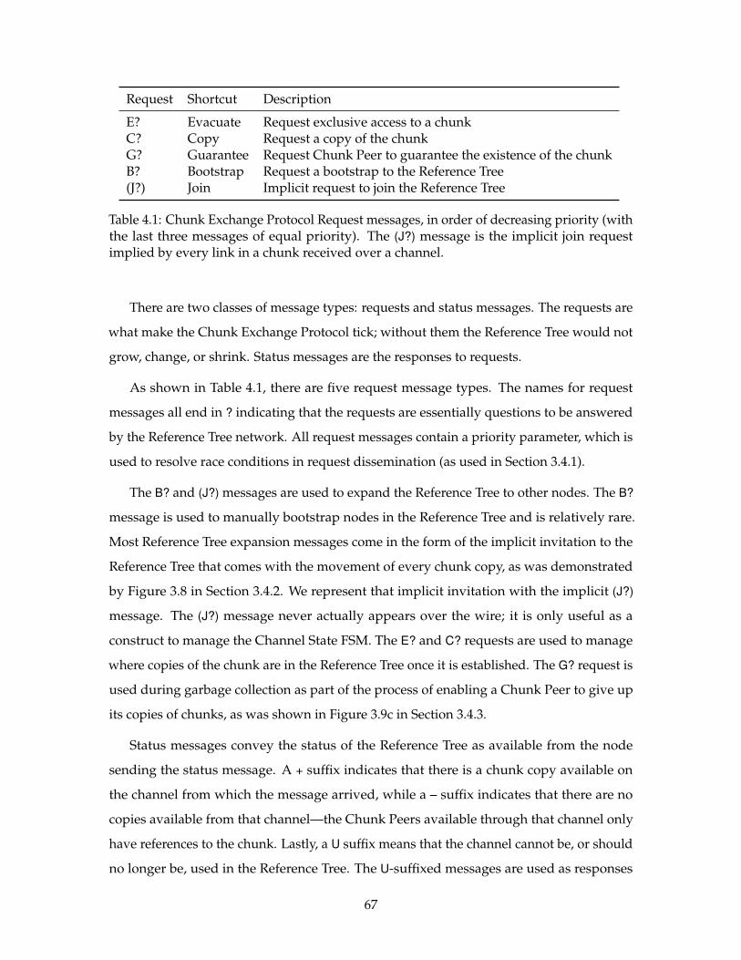
Request Shortcut Description

E? Evacuate Request exclusive access to a chunkC? Copy Request a copy of the chunkG? Guarantee Request Chunk Peer to guarantee the existence of the chunkB? Bootstrap Request a bootstrap to the Reference Tree(J?) Join Implicit request to join the Reference Tree

Table 4.1: Chunk Exchange Protocol Request messages, in order of decreasing priority (withthe last three messages of equal priority). The (J?) message is the implicit join requestimplied by every link in a chunk received over a channel.

There are two classes of message types: requests and status messages. The requests are

what make the Chunk Exchange Protocol tick; without them the Reference Tree would not

grow, change, or shrink. Status messages are the responses to requests.

As shown in Table 4.1, there are five request message types. The names for request

messages all end in ? indicating that the requests are essentially questions to be answered

by the Reference Tree network. All request messages contain a priority parameter, which is

used to resolve race conditions in request dissemination (as used in Section 3.4.1).

The B? and (J?) messages are used to expand the Reference Tree to other nodes. The B?

message is used to manually bootstrap nodes in the Reference Tree and is relatively rare.

Most Reference Tree expansion messages come in the form of the implicit invitation to the

Reference Tree that comes with the movement of every chunk copy, as was demonstrated

by Figure 3.8 in Section 3.4.2. We represent that implicit invitation with the implicit (J?)

message. The (J?) message never actually appears over the wire; it is only useful as a

construct to manage the Channel State FSM. The E? and C? requests are used to manage

where copies of the chunk are in the Reference Tree once it is established. The G? request is

used during garbage collection as part of the process of enabling a Chunk Peer to give up

its copies of chunks, as was shown in Figure 3.9c in Section 3.4.3.

Status messages convey the status of the Reference Tree as available from the node

sending the status message. A + suffix indicates that there is a chunk copy available on

the channel from which the message arrived, while a – suffix indicates that there are no

copies available from that channel—the Chunk Peers available through that channel only

have references to the chunk. Lastly, a U suffix means that the channel cannot be, or should

no longer be, used in the Reference Tree. The U-suffixed messages are used as responses

67

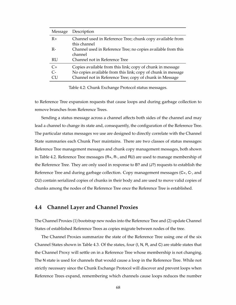
Message Description

R+ Channel used in Reference Tree; chunk copy available fromthis channel

R- Channel used in Reference Tree; no copies available from thischannel

RU Channel not in Reference Tree

C+ Copies available from this link; copy of chunk in messageC- No copies available from this link; copy of chunk in messageCU Channel not in Reference Tree; copy of chunk in Message

Table 4.2: Chunk Exchange Protocol status messages.

to Reference Tree expansion requests that cause loops and during garbage collection to

remove branches from Reference Trees.

Sending a status message across a channel affects both sides of the channel and may

lead a channel to change its state and, consequently, the configuration of the Reference Tree.

The particular status messages we use are designed to directly correlate with the Channel

State summaries each Chunk Peer maintains. There are two classes of status messages:

Reference Tree management messages and chunk copy management messages, both shown

in Table 4.2. Reference Tree messages (R+, R-, and RU) are used to manage membership of

the Reference Tree. They are only used in response to B? and (J?) requests to establish the

Reference Tree and during garbage collection. Copy management messages (C+, C-, and

CU) contain serialized copies of chunks in their body and are used to move valid copies of

chunks among the nodes of the Reference Tree once the Reference Tree is established.

4.4 Channel Layer and Channel Proxies

The Channel Proxies (1) bootstrap new nodes into the Reference Tree and (2) update Channel

States of established Reference Trees as copies migrate between nodes of the tree.

The Channel Proxies summarize the state of the Reference Tree using one of the six

Channel States shown in Table 4.3. Of the states, four (I, N, R, and C) are stable states that

the Channel Proxy will settle on in a Reference Tree whose membership is not changing.

The N state is used for channels that would cause a loop in the Reference Tree. While not

strictly necessary since the Chunk Exchange Protocol will discover and prevent loops when

Reference Trees expand, remembering which channels cause loops reduces the number

68

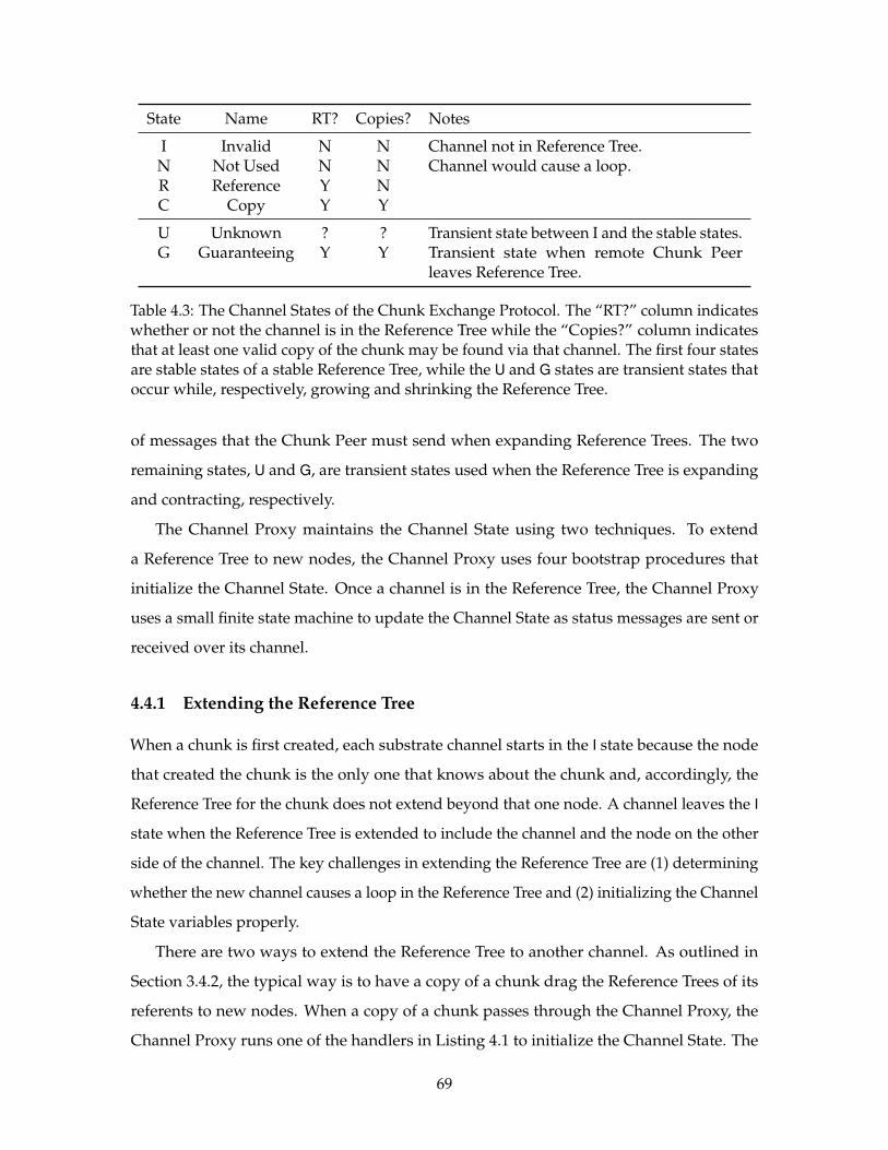
State Name RT? Copies? Notes

I Invalid N N Channel not in Reference Tree.N Not Used N N Channel would cause a loop.R Reference Y NC Copy Y Y

U Unknown ? ? Transient state between I and the stable states.G Guaranteeing Y Y Transient state when remote Chunk Peer

leaves Reference Tree.

Table 4.3: The Channel States of the Chunk Exchange Protocol. The “RT?” column indicateswhether or not the channel is in the Reference Tree while the “Copies?” column indicatesthat at least one valid copy of the chunk may be found via that channel. The first four statesare stable states of a stable Reference Tree, while the U and G states are transient states thatoccur while, respectively, growing and shrinking the Reference Tree.

of messages that the Chunk Peer must send when expanding Reference Trees. The two

remaining states, U and G, are transient states used when the Reference Tree is expanding

and contracting, respectively.

The Channel Proxy maintains the Channel State using two techniques. To extend

a Reference Tree to new nodes, the Channel Proxy uses four bootstrap procedures that

initialize the Channel State. Once a channel is in the Reference Tree, the Channel Proxy

uses a small finite state machine to update the Channel State as status messages are sent or

received over its channel.

4.4.1 Extending the Reference Tree

When a chunk is first created, each substrate channel starts in the I state because the node

that created the chunk is the only one that knows about the chunk and, accordingly, the

Reference Tree for the chunk does not extend beyond that one node. A channel leaves the I

state when the Reference Tree is extended to include the channel and the node on the other

side of the channel. The key challenges in extending the Reference Tree are (1) determining

whether the new channel causes a loop in the Reference Tree and (2) initializing the Channel

State variables properly.

There are two ways to extend the Reference Tree to another channel. As outlined in

Section 3.4.2, the typical way is to have a copy of a chunk drag the Reference Trees of its

referents to new nodes. When a copy of a chunk passes through the Channel Proxy, the

Channel Proxy runs one of the handlers in Listing 4.1 to initialize the Channel State. The

69

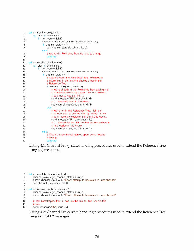
1 def on_send_chunk(chunk):2 for slot in chunk.slots:3 if slot .type == LINK:4 channel_state = get_channel_state(slot.chunk_id)5 if channel_state == I:6 set_channel_state(slot.chunk_id, U)7 else:8 # Already in Reference Tree, no need to change9 continue

1011 def on_receive_chunk(chunk):12 for slot in chunk.slots:13 if slot .type == LINK:14 channel_state = get_channel_state(slot.chunk_id)15 if channel_state == I:16 # Channel not in the Reference Tree. We need to17 # figure out if the channel causes a loop in the18 # Reference Tree.19 if already_in_rt( slot .chunk_id):20 # We're already in the Reference Tree; adding this21 # channel would cause a loop. Tell our network22 # peer not to use the link ...23 send_message("RU", slot.chunk_id)24 # ... and don't use it ourselves:25 set_channel_state(slot.chunk_id, N)26 else:27 # We're not in the Reference Tree. Tell our28 # network peer to use the link by telling it we29 # don't have any copies of the chunk this way)...30 send_message("R−", slot.chunk_id)31 # ... and set up the link so that we know where to32 # find copies of the chunk33 set_channel_state(slot.chunk_id, C)34 else:35 # Channel state already agreed upon, so no need to36 # change.37 continue

Listing 4.1: Channel Proxy state handling procedures used to extend the Reference Treeusing (J?) messages.

1 def on_send_bootstrap(chunk_id):2 channel_state = get_channel_state(chunk_id)3 assert channel_state == I, "Error: attempt to bootstrap in−use channel"4 set_channel_state(chunk_id, U)56 def on_receive_bootstrap(chunk_id):7 channel_state = get_channel_state(chunk_id)8 assert channel_state == I, "Error: attempt to bootstrap in−use channel"9

10 # Tell bootstrapper that it can use the link to find chunks this11 # way12 send_message("R+", chunk_id)

Listing 4.2: Channel Proxy state handling procedures used to extend the Reference Treeusing explicit B? messages.

70

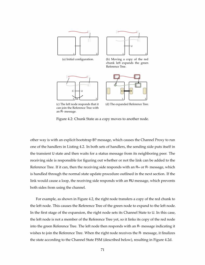
1 2

(a) Initial configuration.

1 2

U

(b) Moving a copy of the redchunk left expands the greenReference Tree.

1 2

C U

R-

(c) The left node responds that itcan join the Reference Tree withan R- message.

1 2

C R

(d) The expanded Reference Tree.

Figure 4.2: Chunk State as a copy moves to another node.

other way is with an explicit bootstrap B? message, which causes the Channel Proxy to run

one of the handlers in Listing 4.2. In both sets of handlers, the sending side puts itself in

the transient U state and then waits for a status message from its neighboring peer. The

receiving side is responsible for figuring out whether or not the link can be added to the

Reference Tree. If it can, then the receiving side responds with an R+ or R- message, which

is handled through the normal state update procedure outlined in the next section. If the

link would cause a loop, the receiving side responds with an RU message, which prevents

both sides from using the channel.

For example, as shown in Figure 4.2, the right node transfers a copy of the red chunk to

the left node. This causes the Reference Tree of the green node to expand to the left node.

In the first stage of the expansion, the right node sets its Channel State to U. In this case,

the left node is not a member of the Reference Tree yet, so it links its copy of the red node

into the green Reference Tree. The left node then responds with an R- message indicating it

wishes to join the Reference Tree. When the right node receives the R- message, it finalizes

the state according to the Channel State FSM (described below), resulting in Figure 4.2d.

71

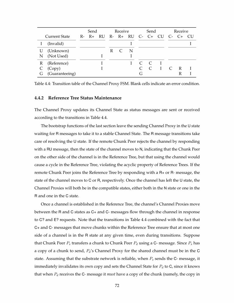
Send Receive Send ReceiveCurrent State R- R+ RU R- R+ RU C- C+ CU C- C+ CU

I (Invalid) I I

U (Unknown) R C NN (Not Used) I I

R (Reference) I I C C IC (Copy) I C C I C R IG (Guaranteeing) G R I

Table 4.4: Transition table of the Channel Proxy FSM. Blank cells indicate an error condition.

4.4.2 Reference Tree Status Maintenance

The Channel Proxy updates its Channel State as status messages are sent or received

according to the transitions in Table 4.4.

The bootstrap functions of the last section leave the sending Channel Proxy in the U state

waiting for R messages to take it to a stable Channel State. The R message transitions take

care of resolving the U state. If the remote Chunk Peer rejects the channel by responding

with a RU message, then the state of the channel moves to N, indicating that the Chunk Peer

on the other side of the channel is in the Reference Tree, but that using the channel would

cause a cycle in the Reference Tree, violating the acyclic property of Reference Trees. If the

remote Chunk Peer joins the Reference Tree by responding with a R+ or R- message, the

state of the channel moves to C or R, respectively. Once the channel has left the U state, the

Channel Proxies will both be in the compatible states, either both in the N state or one in the

R and one in the C state.

Once a channel is established in the Reference Tree, the channel’s Channel Proxies move

between the R and C states as C+ and C- messages flow through the channel in response

to C? and E? requests. Note that the transitions in Table 4.4 combined with the fact that

C+ and C- messages that move chunks within the Reference Tree ensure that at most one

side of a channel is in the R state at any given time, even during transitions. Suppose

that Chunk Peer Ps transfers a chunk to Chunk Peer Pd using a C- message. Since Ps has

a copy of a chunk to send, Pd’s Channel Proxy for the shared channel must be in the C

state. Assuming that the substrate network is reliable, when Ps sends the C- message, it

immediately invalidates its own copy and sets the Channel State for Pd to C, since it knows

that when Pd receives the C- message it must have a copy of the chunk (namely, the copy in

72

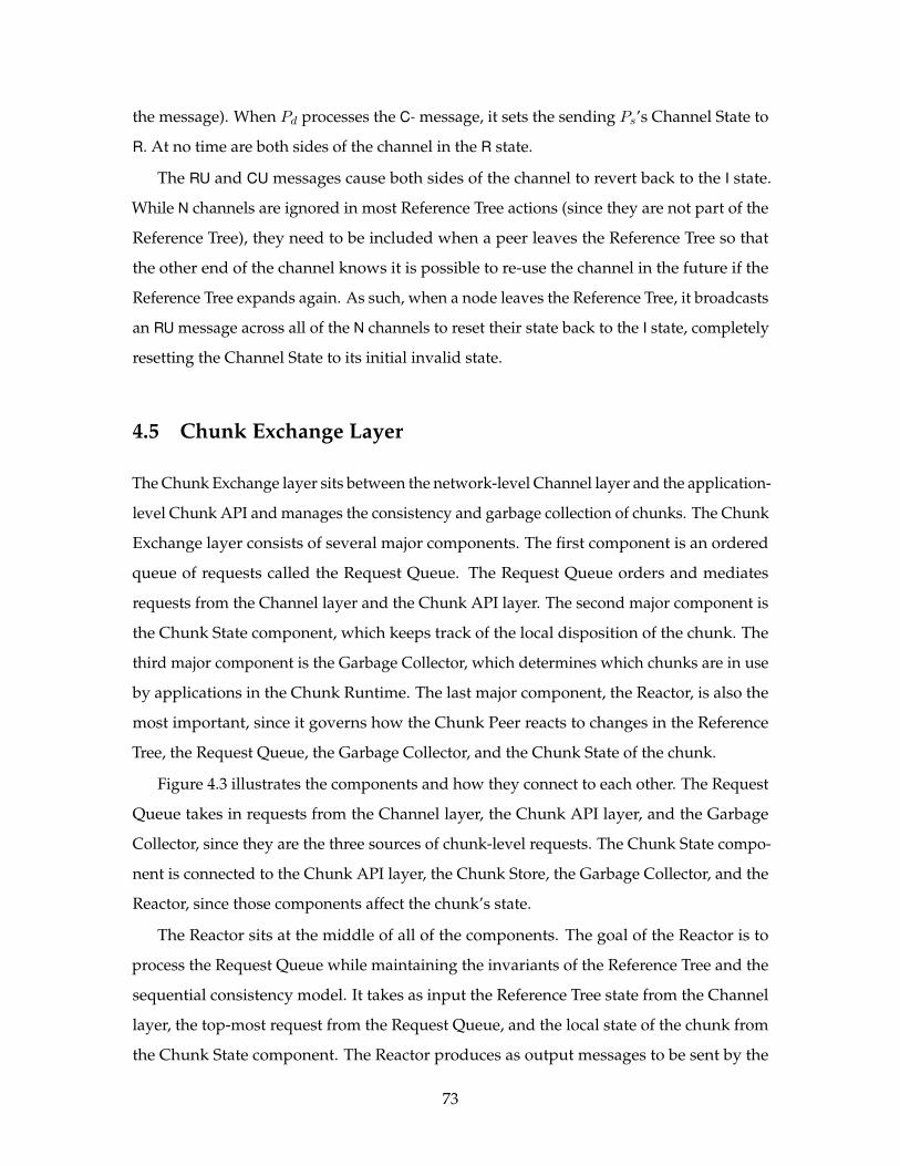
the message). When Pd processes the C- message, it sets the sending Ps’s Channel State to

R. At no time are both sides of the channel in the R state.

The RU and CU messages cause both sides of the channel to revert back to the I state.

While N channels are ignored in most Reference Tree actions (since they are not part of the

Reference Tree), they need to be included when a peer leaves the Reference Tree so that

the other end of the channel knows it is possible to re-use the channel in the future if the

Reference Tree expands again. As such, when a node leaves the Reference Tree, it broadcasts

an RU message across all of the N channels to reset their state back to the I state, completely

resetting the Channel State to its initial invalid state.

4.5 Chunk Exchange Layer

The Chunk Exchange layer sits between the network-level Channel layer and the application-

level Chunk API and manages the consistency and garbage collection of chunks. The Chunk

Exchange layer consists of several major components. The first component is an ordered

queue of requests called the Request Queue. The Request Queue orders and mediates

requests from the Channel layer and the Chunk API layer. The second major component is

the Chunk State component, which keeps track of the local disposition of the chunk. The

third major component is the Garbage Collector, which determines which chunks are in use

by applications in the Chunk Runtime. The last major component, the Reactor, is also the

most important, since it governs how the Chunk Peer reacts to changes in the Reference

Tree, the Request Queue, the Garbage Collector, and the Chunk State of the chunk.

Figure 4.3 illustrates the components and how they connect to each other. The Request

Queue takes in requests from the Channel layer, the Chunk API layer, and the Garbage

Collector, since they are the three sources of chunk-level requests. The Chunk State compo-

nent is connected to the Chunk API layer, the Chunk Store, the Garbage Collector, and the

Reactor, since those components affect the chunk’s state.

The Reactor sits at the middle of all of the components. The goal of the Reactor is to

process the Request Queue while maintaining the invariants of the Reference Tree and the

sequential consistency model. It takes as input the Reference Tree state from the Channel

layer, the top-most request from the Request Queue, and the local state of the chunk from

the Chunk State component. The Reactor produces as output messages to be sent by the

73

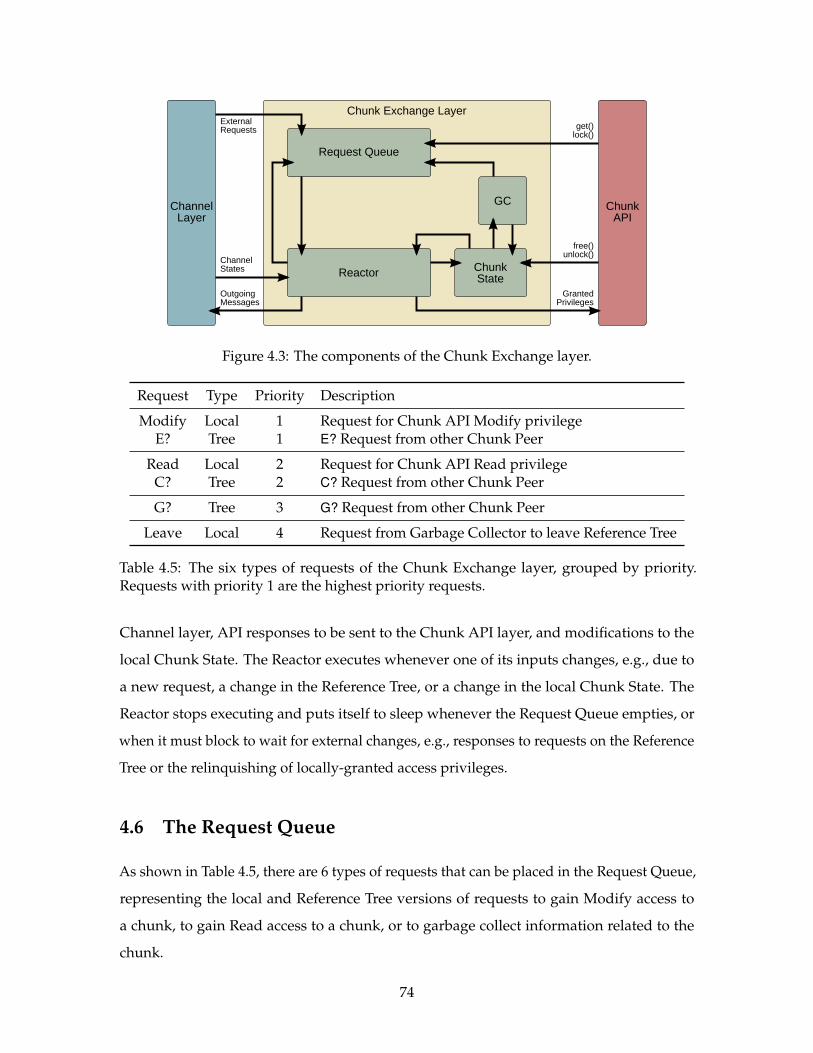
Reactor

ChannelLayer

Request Queue

ChunkState

GC ChunkAPI

get()lock()

free()unlock()

GrantedPrivileges

ExternalRequests

OutgoingMessages

Chunk Exchange Layer

ChannelStates

Figure 4.3: The components of the Chunk Exchange layer.

Request Type Priority Description

Modify Local 1 Request for Chunk API Modify privilegeE? Tree 1 E? Request from other Chunk Peer

Read Local 2 Request for Chunk API Read privilegeC? Tree 2 C? Request from other Chunk Peer

G? Tree 3 G? Request from other Chunk Peer

Leave Local 4 Request from Garbage Collector to leave Reference Tree

Table 4.5: The six types of requests of the Chunk Exchange layer, grouped by priority.Requests with priority 1 are the highest priority requests.

Channel layer, API responses to be sent to the Chunk API layer, and modifications to the

local Chunk State. The Reactor executes whenever one of its inputs changes, e.g., due to

a new request, a change in the Reference Tree, or a change in the local Chunk State. The

Reactor stops executing and puts itself to sleep whenever the Request Queue empties, or

when it must block to wait for external changes, e.g., responses to requests on the Reference

Tree or the relinquishing of locally-granted access privileges.

4.6 The Request Queue

As shown in Table 4.5, there are 6 types of requests that can be placed in the Request Queue,

representing the local and Reference Tree versions of requests to gain Modify access to

a chunk, to gain Read access to a chunk, or to garbage collect information related to the

chunk.

74

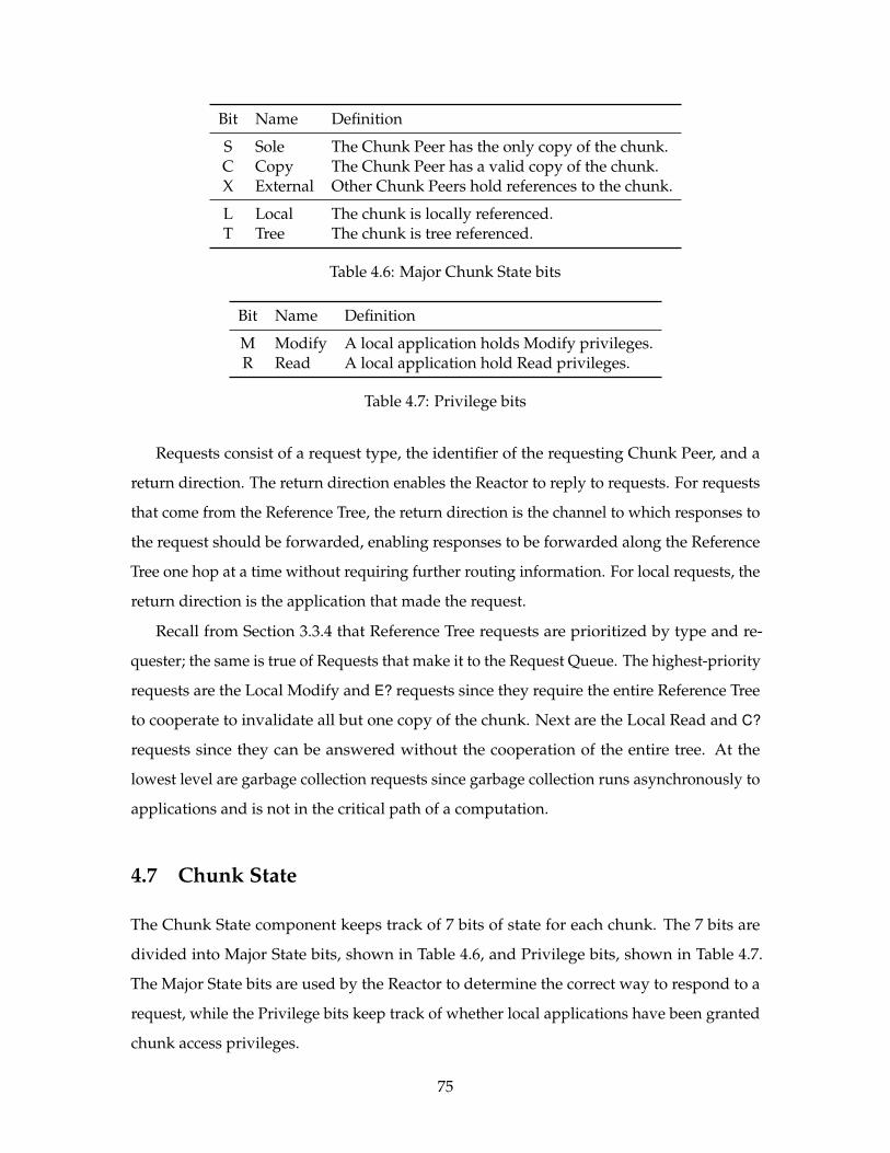
Bit Name Definition

S Sole The Chunk Peer has the only copy of the chunk.C Copy The Chunk Peer has a valid copy of the chunk.X External Other Chunk Peers hold references to the chunk.

L Local The chunk is locally referenced.T Tree The chunk is tree referenced.

Table 4.6: Major Chunk State bits

Bit Name Definition

M Modify A local application holds Modify privileges.R Read A local application hold Read privileges.

Table 4.7: Privilege bits

Requests consist of a request type, the identifier of the requesting Chunk Peer, and a

return direction. The return direction enables the Reactor to reply to requests. For requests

that come from the Reference Tree, the return direction is the channel to which responses to

the request should be forwarded, enabling responses to be forwarded along the Reference

Tree one hop at a time without requiring further routing information. For local requests, the

return direction is the application that made the request.

Recall from Section 3.3.4 that Reference Tree requests are prioritized by type and re-

quester; the same is true of Requests that make it to the Request Queue. The highest-priority

requests are the Local Modify and E? requests since they require the entire Reference Tree

to cooperate to invalidate all but one copy of the chunk. Next are the Local Read and C?

requests since they can be answered without the cooperation of the entire tree. At the

lowest level are garbage collection requests since garbage collection runs asynchronously to

applications and is not in the critical path of a computation.

4.7 Chunk State

The Chunk State component keeps track of 7 bits of state for each chunk. The 7 bits are

divided into Major State bits, shown in Table 4.6, and Privilege bits, shown in Table 4.7.

The Major State bits are used by the Reactor to determine the correct way to respond to a

request, while the Privilege bits keep track of whether local applications have been granted

chunk access privileges.

75

The Major State bits are sub-divided into two categories. The S, C, and X bits summarize

the state of the chunk with respect to its Reference Tree. The X (eXternal) bit is set if any

Channel Proxy is in the R, C, or G state; that is, the X bit is set if the Reference Tree extends

beyond the local node. The C (Copy) bit is set when the Chunk Store contains a valid copy

of the chunk. When the copy is invalidated for consistency reasons, the copy is deleted

from the local Chunk Store and the C bit is cleared. The S (Sole) bit is set when the local

Chunk Peer contains the only copy of the chunk in the Reference Tree. In other words, if

any Channel Proxy is in the C or G state, then S is cleared.

The L and T bits are used to keep track of “liveness” of the Reference Tree by the

Garbage Collector. They are described in detail in Section 4.9, but now it suffices to say that

if either L or T are set, the chunk and its Reference Tree are considered alive by the Garbage

Collector, while if they are both cleared, the chunk and its Reference Tree are candidates for

reclamation.

All seven of the Chunk State bits serve to organize how the Reactor can respond to

a top level request. For example, the Reactor can only grant Read privileges to a local

application if C ·M is true, since the Chunk Peer needs a copy of the chunk to return and no

other application can have Modify privileges. Similarly, the Reactor can only grant Modify

privileges if S ·M · R is true since the Chunk Platform’s sequential consistency memory

model requires that Modify privileges be granted to only one application at a time and that

that application’s Chunk Peer have the sole copy of the chunk. The Chunk State bits also

help guard against garbage collection issues: a node cannot leave the Reference Tree if S · X

is true, since one of the other nodes in the Reference Tree may need to read the sole copy of

the chunk held locally.

Of the 32 possible combinations of Major State bits, the Chunk Exchange layer only uses

17. The Chunk States where S, C, and X are all zero indicate an invalid chunk ID since if the

S, C, and X bits are all cleared, the Chunk Peer has a chunk ID that is not available locally

nor over the Reference Tree. The Chunk Runtime reserves the case where all of the state

bits are zero to indicate a “bad chunk ID”; the other three cases are unused and will signal a

programming error if encountered.

The rest of the unused states derive from the overlap in meaning of the S and C bits. If S

is set, the Chunk Peer has the sole copy of a chunk, which implies that the C bit must also

be set. As such, any state where S is set and C is cleared is treated as an error state. Similarly,

76

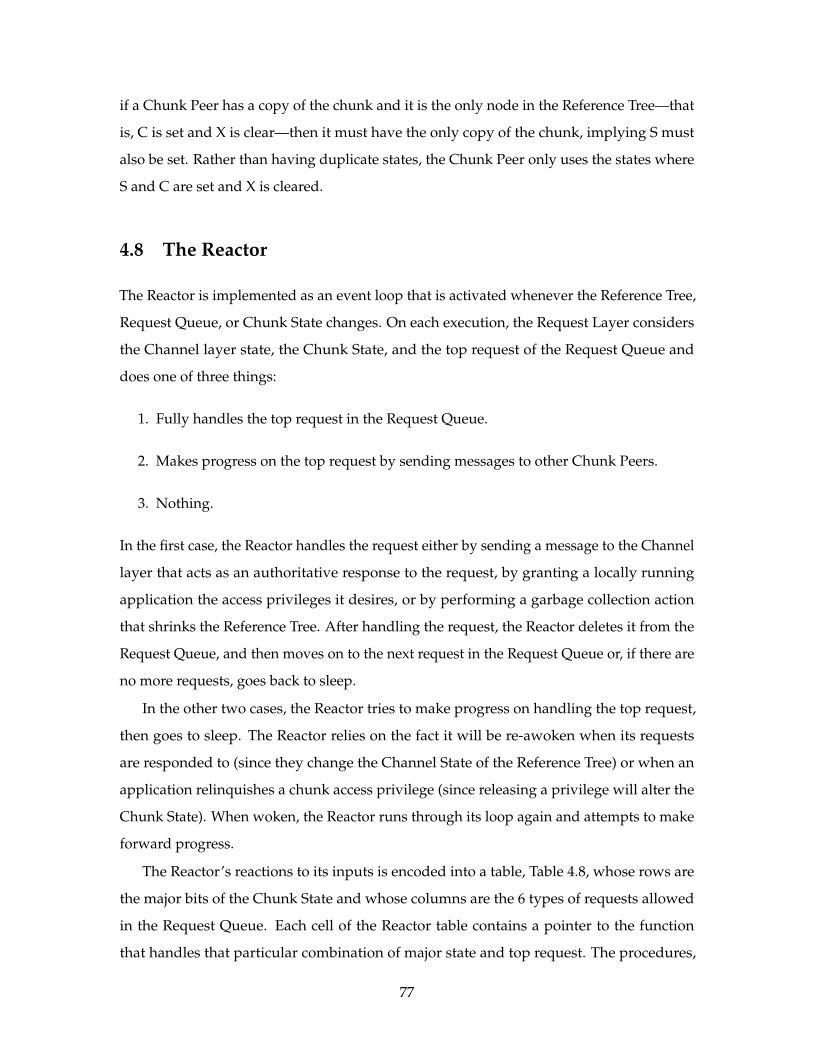
if a Chunk Peer has a copy of the chunk and it is the only node in the Reference Tree—that

is, C is set and X is clear—then it must have the only copy of the chunk, implying S must

also be set. Rather than having duplicate states, the Chunk Peer only uses the states where

S and C are set and X is cleared.

4.8 The Reactor

The Reactor is implemented as an event loop that is activated whenever the Reference Tree,

Request Queue, or Chunk State changes. On each execution, the Request Layer considers

the Channel layer state, the Chunk State, and the top request of the Request Queue and

does one of three things:

1. Fully handles the top request in the Request Queue.

2. Makes progress on the top request by sending messages to other Chunk Peers.

3. Nothing.

In the first case, the Reactor handles the request either by sending a message to the Channel

layer that acts as an authoritative response to the request, by granting a locally running

application the access privileges it desires, or by performing a garbage collection action

that shrinks the Reference Tree. After handling the request, the Reactor deletes it from the

Request Queue, and then moves on to the next request in the Request Queue or, if there are

no more requests, goes back to sleep.

In the other two cases, the Reactor tries to make progress on handling the top request,

then goes to sleep. The Reactor relies on the fact it will be re-awoken when its requests

are responded to (since they change the Channel State of the Reference Tree) or when an

application relinquishes a chunk access privilege (since releasing a privilege will alter the

Chunk State). When woken, the Reactor runs through its loop again and attempts to make

forward progress.

The Reactor’s reactions to its inputs is encoded into a table, Table 4.8, whose rows are

the major bits of the Chunk State and whose columns are the 6 types of requests allowed

in the Request Queue. Each cell of the Reactor table contains a pointer to the function

that handles that particular combination of major state and top request. The procedures,

77

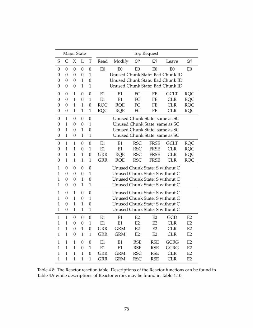
Major State Top Request

S C X L T Read Modify C? E? Leave G?

0 0 0 0 0 E0 E0 E0 E0 E0 E00 0 0 0 1 Unused Chunk State: Bad Chunk ID0 0 0 1 0 Unused Chunk State: Bad Chunk ID0 0 0 1 1 Unused Chunk State: Bad Chunk ID

0 0 1 0 0 E1 E1 FC FE GCLT RQC0 0 1 0 1 E1 E1 FC FE CLR RQC0 0 1 1 0 RQC RQE FC FE CLR RQC0 0 1 1 1 RQC RQE FC FE CLR RQC

0 1 0 0 0 Unused Chunk State: same as SC0 1 0 0 1 Unused Chunk State: same as SC0 1 0 1 0 Unused Chunk State: same as SC0 1 0 1 1 Unused Chunk State: same as SC

0 1 1 0 0 E1 E1 RSC FRSE GCLT RQC0 1 1 0 1 E1 E1 RSC FRSE CLR RQC0 1 1 1 0 GRR RQE RSC FRSE CLR RQC0 1 1 1 1 GRR RQE RSC FRSE CLR RQC

1 0 0 0 0 Unused Chunk State: S without C1 0 0 0 1 Unused Chunk State: S without C1 0 0 1 0 Unused Chunk State: S without C1 0 0 1 1 Unused Chunk State: S without C

1 0 1 0 0 Unused Chunk State: S without C1 0 1 0 1 Unused Chunk State: S without C1 0 1 1 0 Unused Chunk State: S without C1 0 1 1 1 Unused Chunk State: S without C

1 1 0 0 0 E1 E1 E2 E2 GCD E21 1 0 0 1 E1 E1 E2 E2 CLR E21 1 0 1 0 GRR GRM E2 E2 CLR E21 1 0 1 1 GRR GRM E2 E2 CLR E2

1 1 1 0 0 E1 E1 RSE RSE GCRG E21 1 1 0 1 E1 E1 RSE RSE GCRG E21 1 1 1 0 GRR GRM RSC RSE CLR E21 1 1 1 1 GRR GRM RSC RSE CLR E2

Table 4.8: The Reactor reaction table. Descriptions of the Reactor functions can be found inTable 4.9 while descriptions of Reactor errors may be found in Table 4.10.

78

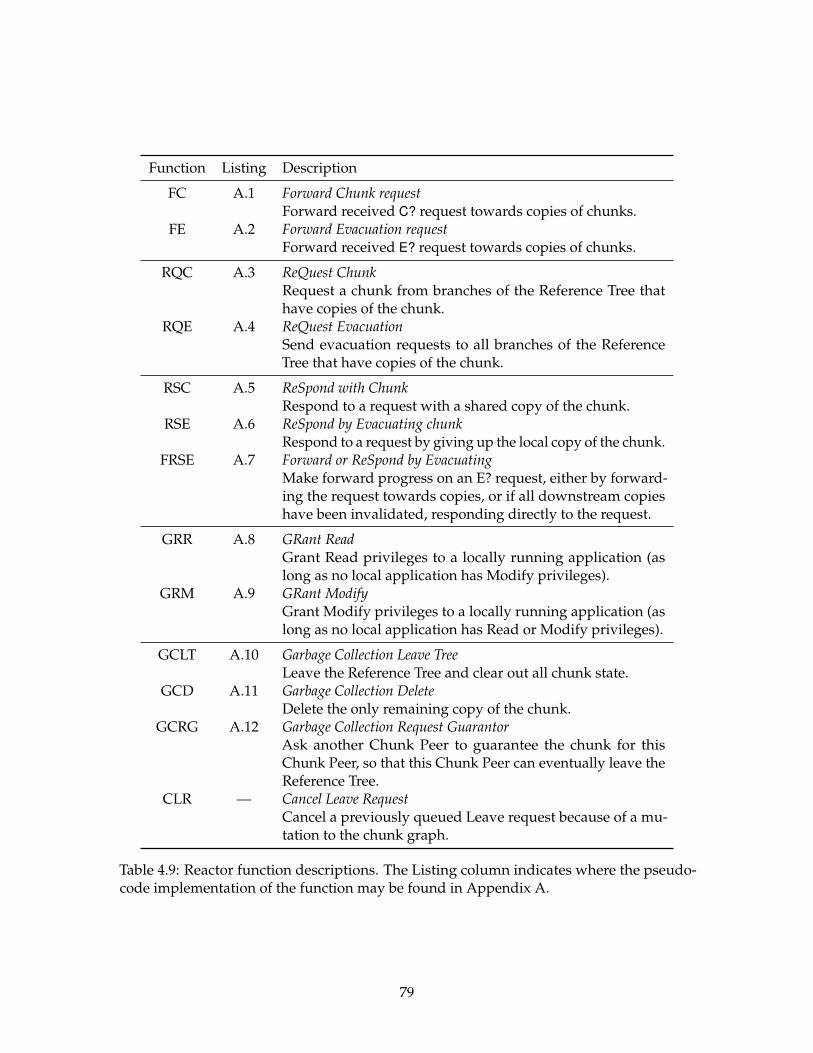
Function Listing Description

FC A.1 Forward Chunk requestForward received C? request towards copies of chunks.

FE A.2 Forward Evacuation requestForward received E? request towards copies of chunks.

RQC A.3 ReQuest ChunkRequest a chunk from branches of the Reference Tree thathave copies of the chunk.

RQE A.4 ReQuest EvacuationSend evacuation requests to all branches of the ReferenceTree that have copies of the chunk.

RSC A.5 ReSpond with ChunkRespond to a request with a shared copy of the chunk.

RSE A.6 ReSpond by Evacuating chunkRespond to a request by giving up the local copy of the chunk.

FRSE A.7 Forward or ReSpond by EvacuatingMake forward progress on an E? request, either by forward-ing the request towards copies, or if all downstream copieshave been invalidated, responding directly to the request.

GRR A.8 GRant ReadGrant Read privileges to a locally running application (aslong as no local application has Modify privileges).

GRM A.9 GRant ModifyGrant Modify privileges to a locally running application (aslong as no local application has Read or Modify privileges).

GCLT A.10 Garbage Collection Leave TreeLeave the Reference Tree and clear out all chunk state.

GCD A.11 Garbage Collection DeleteDelete the only remaining copy of the chunk.

GCRG A.12 Garbage Collection Request GuarantorAsk another Chunk Peer to guarantee the chunk for thisChunk Peer, so that this Chunk Peer can eventually leave theReference Tree.

CLR — Cancel Leave RequestCancel a previously queued Leave request because of a mu-tation to the chunk graph.

Table 4.9: Reactor function descriptions. The Listing column indicates where the pseudo-code implementation of the function may be found in Appendix A.

79

Error Description

E0 Request on an unknown chunk IDE1 Local request without local referenceE2 Tree request without a Reference Tree

Table 4.10: Reactor Error Types

321

SC •

L •

(a) Node 3 creates a new chunk.

321

C R C R• • X

L •

• • X

L •

SCX

LT

(b) State after expanding the Reference Tree to nodes1 and 2.

Figure 4.4: Chunk and Channel States during Reference Tree expansion.

described in Table 4.9 and written out in Appendix A, interact with the Channel Proxies,

Chunk State component, and the Chunk Store.

Certain combinations of Chunk State and request do not make logical sense. The error

conditions, described in Table 4.10 describe why that particular cell is an error condition. The

Chunk Runtime sends an error message to the application or requesting peer in response to

one of the error conditions and then deletes the errant request.

4.8.1 Expanding the Reference Tree

To gain intuition about how the Reactor works, consider the three nodes in Figure 4.4.

Suppose that node 3 creates a new chunk. Newly created chunks start in the S · C · X · L · T

Chunk State since the node that created the chunk has the only copy (S · C), no other node

knows about the chunk yet (X · T), and it is locally referenced since it was just created (L).

Suppose that the Reference Tree expands to encompass the other two nodes. The Reactor

does not handle Reference Tree expansions; instead it is notified by the Channel layer when

new neighbors join the Reference Tree. As shown in Figure 4.4b, only the X and L bits are

set on nodes 1 and 2, as they are members of the Reference Tree and reference, but do not

have copies of, the chunk. Note that the expansion sets the X and T bits on node 3. The

X bit is set because the Reference Tree now expands beyond just node 3. The reasons for

80

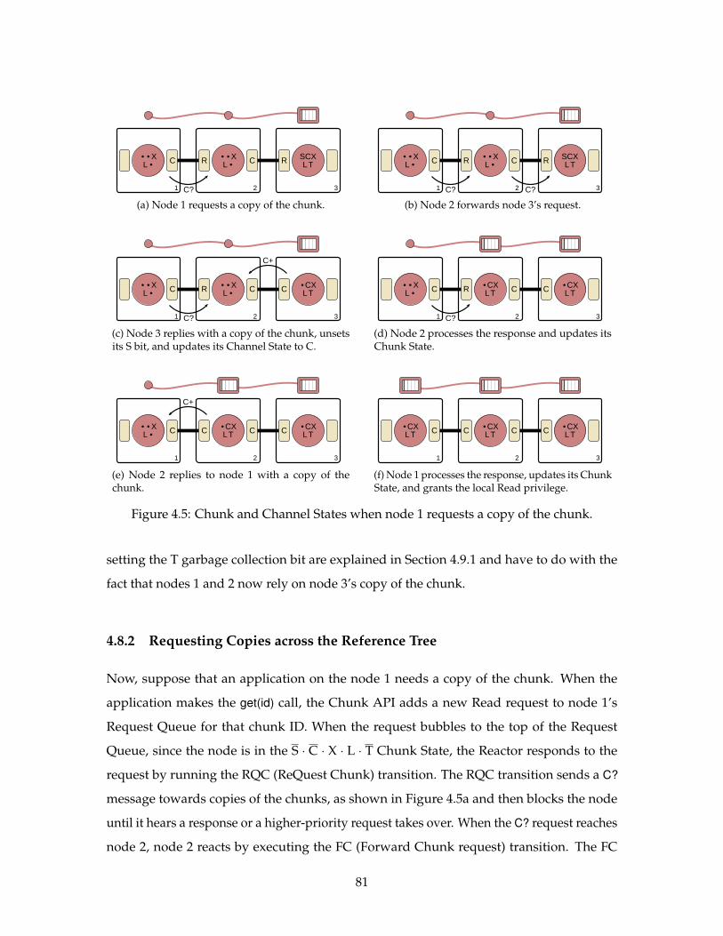
321

C R C R• • X

L •

• • X

L •

SCX

LT

C?

(a) Node 1 requests a copy of the chunk.

321

C R C R• • X

L •

• • X

L •

SCX

LT

C? C?

(b) Node 2 forwards node 3’s request.

321

C R C C• • X

L •

• • X

L •

•CX

LT

C?

C+

(c) Node 3 replies with a copy of the chunk, unsetsits S bit, and updates its Channel State to C.

321

C R C C• • X

L •

•CX

LT

•CX

LT

C?

(d) Node 2 processes the response and updates itsChunk State.

321

C C C C• • X

L •

•CX

LT

•CX

LT

C+

(e) Node 2 replies to node 1 with a copy of thechunk.

321

C C C C•CX

LT

•CX

LT

•CX

LT

(f) Node 1 processes the response, updates its ChunkState, and grants the local Read privilege.

Figure 4.5: Chunk and Channel States when node 1 requests a copy of the chunk.

setting the T garbage collection bit are explained in Section 4.9.1 and have to do with the

fact that nodes 1 and 2 now rely on node 3’s copy of the chunk.

4.8.2 Requesting Copies across the Reference Tree

Now, suppose that an application on the node 1 needs a copy of the chunk. When the

application makes the get(id) call, the Chunk API adds a new Read request to node 1’s

Request Queue for that chunk ID. When the request bubbles to the top of the Request

Queue, since the node is in the S · C · X · L · T Chunk State, the Reactor responds to the

request by running the RQC (ReQuest Chunk) transition. The RQC transition sends a C?

message towards copies of the chunks, as shown in Figure 4.5a and then blocks the node

until it hears a response or a higher-priority request takes over. When the C? request reaches

node 2, node 2 reacts by executing the FC (Forward Chunk request) transition. The FC

81

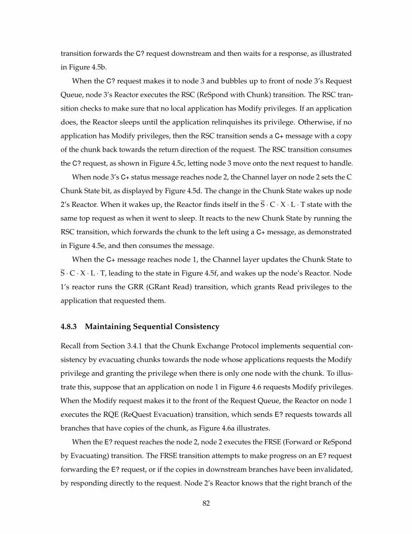
transition forwards the C? request downstream and then waits for a response, as illustrated

in Figure 4.5b.

When the C? request makes it to node 3 and bubbles up to front of node 3’s Request

Queue, node 3’s Reactor executes the RSC (ReSpond with Chunk) transition. The RSC tran-

sition checks to make sure that no local application has Modify privileges. If an application

does, the Reactor sleeps until the application relinquishes its privilege. Otherwise, if no

application has Modify privileges, then the RSC transition sends a C+ message with a copy

of the chunk back towards the return direction of the request. The RSC transition consumes

the C? request, as shown in Figure 4.5c, letting node 3 move onto the next request to handle.

When node 3’s C+ status message reaches node 2, the Channel layer on node 2 sets the C

Chunk State bit, as displayed by Figure 4.5d. The change in the Chunk State wakes up node

2’s Reactor. When it wakes up, the Reactor finds itself in the S · C · X · L · T state with the

same top request as when it went to sleep. It reacts to the new Chunk State by running the

RSC transition, which forwards the chunk to the left using a C+ message, as demonstrated

in Figure 4.5e, and then consumes the message.

When the C+ message reaches node 1, the Channel layer updates the Chunk State to

S · C · X · L · T, leading to the state in Figure 4.5f, and wakes up the node’s Reactor. Node

1’s reactor runs the GRR (GRant Read) transition, which grants Read privileges to the

application that requested them.

4.8.3 Maintaining Sequential Consistency

Recall from Section 3.4.1 that the Chunk Exchange Protocol implements sequential con-

sistency by evacuating chunks towards the node whose applications requests the Modify

privilege and granting the privilege when there is only one node with the chunk. To illus-

trate this, suppose that an application on node 1 in Figure 4.6 requests Modify privileges.

When the Modify request makes it to the front of the Request Queue, the Reactor on node 1

executes the RQE (ReQuest Evacuation) transition, which sends E? requests towards all

branches that have copies of the chunk, as Figure 4.6a illustrates.

When the E? request reaches the node 2, node 2 executes the FRSE (Forward or ReSpond

by Evacuating) transition. The FRSE transition attempts to make progress on an E? request

forwarding the E? request, or if the copies in downstream branches have been invalidated,

by responding directly to the request. Node 2’s Reactor knows that the right branch of the

82

321

C C C C•CX

LT

•CX

LT

•CX

LT

E?

(a) Node 1 requests evacuation of the chunk.

321

C C C C•CX

LT

•CX

LT

•CX

LT

E? E?

(b) Node 2 forwards node 1’s request.

321

C C C C•CX

LT

•CX

LT

• • X

LT

E?

C-

(c) Node 3 replies by deleting its copy of the chunkand sending it to node 2, unsetting its C bit.

321

C C R C•CX

LT

•CX

LT

• • X

LT

E?

(d) Node 2 processes the status message, updatingits Channel State for node 3.

321

C C R C•CX

LT

• • X

LT

• • X

LT

C-

(e) Now that all downstream chunks have been evac-uated, node 2 replies to node 1 by deleting its copyof the chunk, unsetting its C bit, and sending thechunk to node 1.

321

R C R CSCX

LT

• • X

LT

• • X

LT

(f) Node 1 processes the status message, updatesits Chunk and Channel States, and grants the localModify privilege.

Figure 4.6: Chunk and Channel States for the process of granting a Modify request.

83

Reference Tree still has a copy, so the FRSE transition executes the FE (Forward Evacuation

request) branch, which forwards the E? request to the right node, as shown in Figure 4.6b.

When the E? request reaches node 3, the node’s Reactor also executes the FRSE transition.

In this case, the FRSE transition executes the RSE (ReSpond by Evacuating chunk) branch,

since there are no downstream nodes to which to forward the E? request. The RSE branch

waits until local applications relinquish all of their access privileges. When they have,

node 3 invalidates its local copy of the chunk (unsetting the C bit of Chunk State) and then

responds to the original request with an C- message, as demonstrated in Figure 4.6c.

When node 3’s C- message reaches node 2, node 2’s Channel layer sets node 3’s channel

to R (Figure 4.6d) and then forwards the request to the Reactor. Node 2’s Reactor re-runs

the FRSE transition, which now runs the RSE branch since the downstream nodes no longer

have copies of the chunk. Like node 3, node 2 deletes its local chunk copy, clears its C bit,

and then forwards the chunk to the left using a C- message, as Figure 4.6e shows.

When the C- message reaches node 1, the Channel layer resets the Channel State for

the Reference Tree to R, which causes the S bit to be set in the Chunk State, leading to the

configuration shown in Figure 4.6f. When the node 1’s Reactor wakes up, it finds itself in

the S · C · X · L · T state and correspondingly runs the GRM (GRant Modify) transition to

grant the Modify privilege to the application that requested it.

4.9 Garbage Collection

Distributed garbage collection in the Chunk Platform faces two main challenges. The first

is that of maintaining connectivity of Reference Trees. Since Reference Trees connect all

nodes that reference a chunk, a node whose applications no longer use a chunk may be

required to stay in the Reference Tree since it is on the path between other nodes that do

have live references to the chunk. As such, the Chunk Platform must safely determine when

a particular node can leave the Reference Tree safely.

The second challenge is that of asynchrony. Given that modern computing substrates

may be arbitrarily large, it is not feasible to perform globally synchronous garbage collection.

Instead, garbage collection processes that may pause a single node must run in parallel

with other nodes that are actively mutating the global chunk graph. The Chunk Platform

84

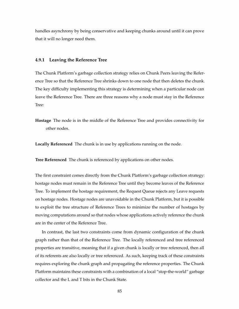
handles asynchrony by being conservative and keeping chunks around until it can prove

that it will no longer need them.

4.9.1 Leaving the Reference Tree

The Chunk Platform’s garbage collection strategy relies on Chunk Peers leaving the Refer-

ence Tree so that the Reference Tree shrinks down to one node that then deletes the chunk.

The key difficulty implementing this strategy is determining when a particular node can

leave the Reference Tree. There are three reasons why a node must stay in the Reference

Tree:

Hostage The node is in the middle of the Reference Tree and provides connectivity for

other nodes.

Locally Referenced The chunk is in use by applications running on the node.

Tree Referenced The chunk is referenced by applications on other nodes.

The first constraint comes directly from the Chunk Platform’s garbage collection strategy:

hostage nodes must remain in the Reference Tree until they become leaves of the Reference

Tree. To implement the hostage requirement, the Request Queue rejects any Leave requests

on hostage nodes. Hostage nodes are unavoidable in the Chunk Platform, but it is possible

to exploit the tree structure of Reference Trees to minimize the number of hostages by

moving computations around so that nodes whose applications actively reference the chunk

are in the center of the Reference Tree.

In contrast, the last two constraints come from dynamic configuration of the chunk

graph rather than that of the Reference Tree. The locally referenced and tree referenced

properties are transitive, meaning that if a given chunk is locally or tree referenced, then all

of its referents are also locally or tree referenced. As such, keeping track of these constraints

requires exploring the chunk graph and propagating the reference properties. The Chunk

Platform maintains these constraints with a combination of a local “stop-the-world” garbage

collector and the L and T bits in the Chunk State.

85

Locally Referenced Chunks

Locally referenced chunks are those that are in use by an application running on the node.

In other words, local referencing is the standard concept of liveness in garbage collected

systems.

The Chunk Peer keeps track of local references through the L bit in the Chunk State

component. As a base case, the L bit is set on any chunk in the garbage collector’s “root

set” of live chunks. This set is modified by applications using the gc_root_add(id) and

gc_root_remove(id) functions of the Chunk API.

The L bit is maintained two ways. First, the L bit is set or cleared by a standard “mark

and sweep” garbage collector, providing a periodic ground truth of liveness. Second,

whenever the Chunk Peer processes a chunk copy whose L bit is set, it automatically sets

the L bit of all of its referents. This lets us handle asynchronous mutation of the chunk graph

during garbage collection since it propagates the L bit as applications walk through the

chunk graph or chunks are transferred by the Channel Layer through the Chunk Peer. This

maintenance strategy is conservative because only the periodic runs of the garbage collector

can clear the L bit. However, conservatism is warranted since leaving the Reference Tree

destroys information.

Tree Referenced Chunks

Tree referenced chunks are those that are live on a particular node in order to ensure

referential integrity of the chunk graph for other nodes. The simplest example of a tree

referenced chunk is an externally-referenced sole copy of a chunk held at a node that wishes

to garbage collect the chunk and leave its Reference Tree. If the node just deletes the chunk,

the node will break the referential integrity of links on other nodes pointing to that chunk.

As such, the node holding the chunk must stay in the Reference Tree until it gives a copy to

another node in the Reference Tree.

More generally, any externally-referenced chunk for which a node has a locally valid

copy is considered tree referenced, since those chunks can be used to satisfy external C?

requests from the Reference Tree. Moreover, every chunk linked by a tree referenced chunk

is tree referenced since the initial tree referenced chunk may point to a sub-graph of chunks

that only the node knows about.

86

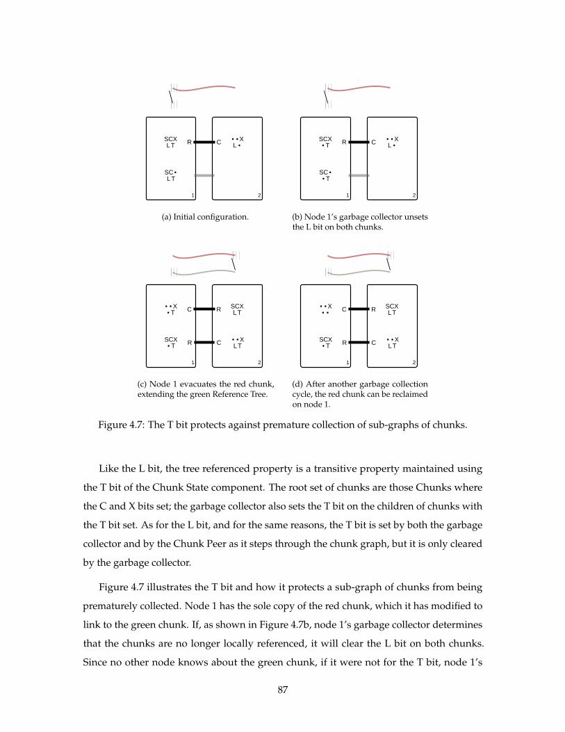
21

R C

SC •

LT

SCX

LT

• • X

L •

(a) Initial configuration.

21

R C

SC •

• T

SCX

• T

• • X

L •

(b) Node 1’s garbage collector unsetsthe L bit on both chunks.

21

R C

C R

SCX

• T

• • X

LT

• • X

• T

SCX

LT

(c) Node 1 evacuates the red chunk,extending the green Reference Tree.

21

R C

C R

SCX

• T

• • X

LT

• • X

• •

SCX

LT

(d) After another garbage collectioncycle, the red chunk can be reclaimedon node 1.

Figure 4.7: The T bit protects against premature collection of sub-graphs of chunks.

Like the L bit, the tree referenced property is a transitive property maintained using

the T bit of the Chunk State component. The root set of chunks are those Chunks where

the C and X bits set; the garbage collector also sets the T bit on the children of chunks with

the T bit set. As for the L bit, and for the same reasons, the T bit is set by both the garbage

collector and by the Chunk Peer as it steps through the chunk graph, but it is only cleared

by the garbage collector.

Figure 4.7 illustrates the T bit and how it protects a sub-graph of chunks from being

prematurely collected. Node 1 has the sole copy of the red chunk, which it has modified to

link to the green chunk. If, as shown in Figure 4.7b, node 1’s garbage collector determines

that the chunks are no longer locally referenced, it will clear the L bit on both chunks.

Since no other node knows about the green chunk, if it were not for the T bit, node 1’s

87

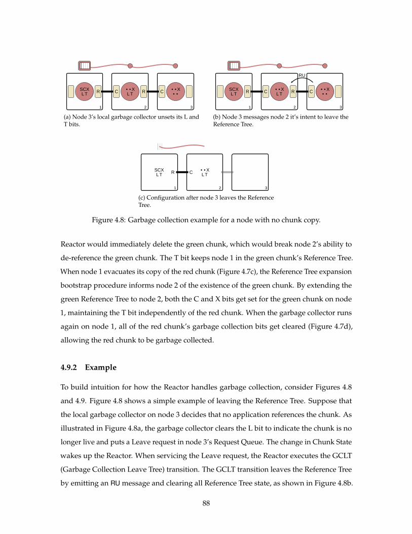
321

R C R CSCX

LT

• • X

LT

• • X

• •

(a) Node 3’s local garbage collector unsets its L andT bits.

321

R C R CSCX

LT

• • X

LT

• • X

• •

RU

(b) Node 3 messages node 2 it’s intent to leave theReference Tree.

321

R CSCX

LT

• • X

LT

(c) Configuration after node 3 leaves the ReferenceTree.

Figure 4.8: Garbage collection example for a node with no chunk copy.

Reactor would immediately delete the green chunk, which would break node 2’s ability to

de-reference the green chunk. The T bit keeps node 1 in the green chunk’s Reference Tree.

When node 1 evacuates its copy of the red chunk (Figure 4.7c), the Reference Tree expansion

bootstrap procedure informs node 2 of the existence of the green chunk. By extending the

green Reference Tree to node 2, both the C and X bits get set for the green chunk on node

1, maintaining the T bit independently of the red chunk. When the garbage collector runs

again on node 1, all of the red chunk’s garbage collection bits get cleared (Figure 4.7d),

allowing the red chunk to be garbage collected.

4.9.2 Example

To build intuition for how the Reactor handles garbage collection, consider Figures 4.8

and 4.9. Figure 4.8 shows a simple example of leaving the Reference Tree. Suppose that

the local garbage collector on node 3 decides that no application references the chunk. As

illustrated in Figure 4.8a, the garbage collector clears the L bit to indicate the chunk is no

longer live and puts a Leave request in node 3’s Request Queue. The change in Chunk State

wakes up the Reactor. When servicing the Leave request, the Reactor executes the GCLT

(Garbage Collection Leave Tree) transition. The GCLT transition leaves the Reference Tree

by emitting an RU message and clearing all Reference Tree state, as shown in Figure 4.8b.

88

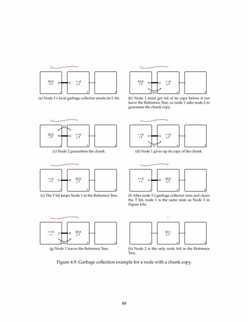
321

R CSCX

• T

• • X

LT

(a) Node 1’s local garbage collector unsets its L bit.

321

R CSCX

• T

• • X

LT

G?

(b) Node 1 must get rid of its copy before it canleave the Reference Tree, so node 1 asks node 2 toguarantee the chunk copy.

321

R GSCX

• T

• • X

LT

C?

(c) Node 2 guarantees the chunk.

321

C G• • X

• T

• • X

LT

C-

(d) Node 1 gives up its copy of the chunk.

321

C R• • X

• T

SCX

LT

(e) The T bit keeps Node 1 in the Reference Tree.

321

C R• • X

• •

SCX

LT

(f) After node 1’s garbage collector runs and clearsthe T bit, node 1 is the same state as Node 3 inFigure 4.8a.

321

C R• • X

• •

SCX

LT

RU

(g) Node 1 leaves the Reference Tree.

321

SC •

LT

(h) Node 2 is the only node left in the ReferenceTree.

Figure 4.9: Garbage collection example for a node with a chunk copy.

89

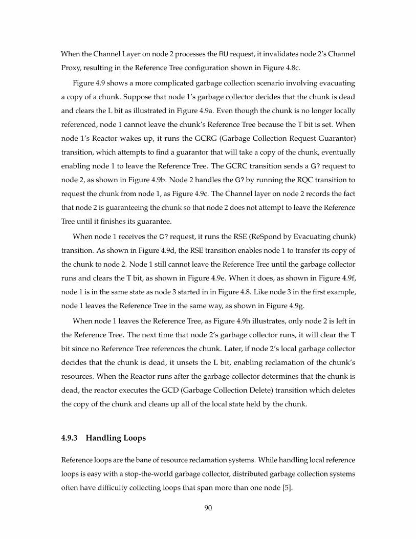
When the Channel Layer on node 2 processes the RU request, it invalidates node 2’s Channel

Proxy, resulting in the Reference Tree configuration shown in Figure 4.8c.

Figure 4.9 shows a more complicated garbage collection scenario involving evacuating

a copy of a chunk. Suppose that node 1’s garbage collector decides that the chunk is dead

and clears the L bit as illustrated in Figure 4.9a. Even though the chunk is no longer locally

referenced, node 1 cannot leave the chunk’s Reference Tree because the T bit is set. When

node 1’s Reactor wakes up, it runs the GCRG (Garbage Collection Request Guarantor)

transition, which attempts to find a guarantor that will take a copy of the chunk, eventually

enabling node 1 to leave the Reference Tree. The GCRC transition sends a G? request to

node 2, as shown in Figure 4.9b. Node 2 handles the G? by running the RQC transition to

request the chunk from node 1, as Figure 4.9c. The Channel layer on node 2 records the fact

that node 2 is guaranteeing the chunk so that node 2 does not attempt to leave the Reference

Tree until it finishes its guarantee.

When node 1 receives the C? request, it runs the RSE (ReSpond by Evacuating chunk)

transition. As shown in Figure 4.9d, the RSE transition enables node 1 to transfer its copy of

the chunk to node 2. Node 1 still cannot leave the Reference Tree until the garbage collector

runs and clears the T bit, as shown in Figure 4.9e. When it does, as shown in Figure 4.9f,

node 1 is in the same state as node 3 started in in Figure 4.8. Like node 3 in the first example,

node 1 leaves the Reference Tree in the same way, as shown in Figure 4.9g.

When node 1 leaves the Reference Tree, as Figure 4.9h illustrates, only node 2 is left in

the Reference Tree. The next time that node 2’s garbage collector runs, it will clear the T

bit since no Reference Tree references the chunk. Later, if node 2’s local garbage collector

decides that the chunk is dead, it unsets the L bit, enabling reclamation of the chunk’s

resources. When the Reactor runs after the garbage collector determines that the chunk is

dead, the reactor executes the GCD (Garbage Collection Delete) transition which deletes

the copy of the chunk and cleans up all of the local state held by the chunk.

4.9.3 Handling Loops

Reference loops are the bane of resource reclamation systems. While handling local reference

loops is easy with a stop-the-world garbage collector, distributed garbage collection systems

often have difficulty collecting loops that span more than one node [5].

90

21

C R

R C

• • X

LT

SCX

LT

SCX

LT

• • X

LT

(a) Reference loop spanning twonodes.

21

C R

R C

• • X

• T

SCX

LT

SCX

• T

• • X

LT

(b) Even after clearing the L bit, node1 has a T-bit loop.

21

C R

C R

• • X

• T

SCX

LT

• • X

• T

SCX

LT

(c) Evacuating the red chunk to node2 clears the C bit on node 1.

21

C R

C R

• • X

• •

SCX

LT

• • X

• •

SCX

LT

(d) After node 1’s garbage collectorruns again, the T bits are clear.

Figure 4.10: A cycle spanning multiple nodes.

The key to collecting distributed reference loops is finding a way to break the loops

between the nodes. In the Chunk Platform, distributed loops are loops formed by chunks in

Chunk States where L ·T is true, since chunks with the L bit set are locally live and won’t be

touched by the garbage collector, while chunks in Chunk States where L · T is true are not

referenced at all and can be reclaimed without further ado. Since the T bit is set on chunks

where C ·X is true, the Chunk Peer breaks loops by evacuating chunks to other nodes in the

Reference Tree. By evacuating chunks, the Chunk Peer reduces the set of chunks that have

the C Chunk State bit set, transitively reducing the set of chunks that have the T Chunk

State bit set.

Consider the cycle in Figure 4.10a that spans two nodes. Suppose that node 1’s garbage

collector decides that both chunks are dead, leading to the T-bit loop in Figure 4.10b. If

node 1 evacuates the red chunk to node 2, node 1 can clear the red chunk’s C bit, as shown

91

in Figure 4.10c. When node 1’s garbage collector runs again, it will clear the T bit on

both chunks since no C · X or T chunks point to either of them, leading to the situation in

Figure 4.10d. As this point, the loop is completely broken and node 1 can leave both chunks’

Reference Trees.

92

Chapter 5

Applications

A main claim of this thesis is that structured computing models like the Chunk Model make

it easier to build and maintain applications, and the run-time systems that support those

applications, on modern computing substrates. The evaluate that claim, this chapter details

three applications built on top of our Chunk Platform implementation of the Chunk Model.

The first application, SCVM, serves as a vehicle for evaluating the general applicability

of the Chunk Model as a compute platform. SCVM demonstrates the claim that the Chunk

Model is suitably application-generic by supporting a general-purpose compiler as well

as two SCVM-based applications that successfully use SCVM’s machine model to achieve

their tasks. The second application, Tasklets, uses the Chunk Platform and SCVM to

build infrastructure for offloading small computation tasks to the cloud. Tasklets further

demonstrate the application-generic nature of chunks by proposing a new model for cloud

computing. The last application, ChunkStream, serves as a vehicle for chunks as a data-only

model. ChunkStream demonstrates the claim that the Chunk Model is transparent and can

be adapted to real-world uses of complex data types.

5.1 SCVM

SCVM is a chunk-oriented virtual machine that uses the CVM data structure of Section 2.3.2.

As an evaluation mechanism, SCVM serves two purposes. First, it shows chunks to be

a suitable foundation for computation. Second, it serves as an example application that

stresses the Chunk Platform, and indeed drove much of the development of system-level

features like sequential consistency and garbage collection.

93

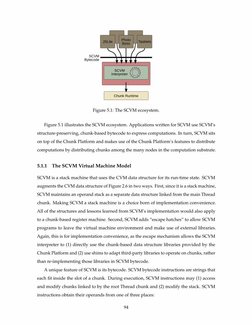
JSLitePhotoBoss

Tasklets

Chunk Runtime

SCVMBytecode

SCVMInterpreter

Figure 5.1: The SCVM ecosystem.

Figure 5.1 illustrates the SCVM ecosystem. Applications written for SCVM use SCVM’s

structure-preserving, chunk-based bytecode to express computations. In turn, SCVM sits

on top of the Chunk Platform and makes use of the Chunk Platform’s features to distribute

computations by distributing chunks among the many nodes in the computation substrate.

5.1.1 The SCVM Virtual Machine Model

SCVM is a stack machine that uses the CVM data structure for its run-time state. SCVM

augments the CVM data structure of Figure 2.6 in two ways. First, since it is a stack machine,

SCVM maintains an operand stack as a separate data structure linked from the main Thread

chunk. Making SCVM a stack machine is a choice born of implementation convenience.

All of the structures and lessons learned from SCVM’s implementation would also apply

to a chunk-based register machine. Second, SCVM adds “escape hatches” to allow SCVM

programs to leave the virtual machine environment and make use of external libraries.

Again, this is for implementation convenience, as the escape mechanism allows the SCVM

interpreter to (1) directly use the chunk-based data structure libraries provided by the

Chunk Platform and (2) use shims to adapt third-party libraries to operate on chunks, rather

than re-implementing those libraries in SCVM bytecode.

A unique feature of SCVM is its bytecode. SCVM bytecode instructions are strings that

each fit inside the slot of a chunk. During execution, SCVM instructions may (1) access

and modify chunks linked to by the root Thread chunk and (2) modify the stack. SCVM

instructions obtain their operands from one of three places:

94

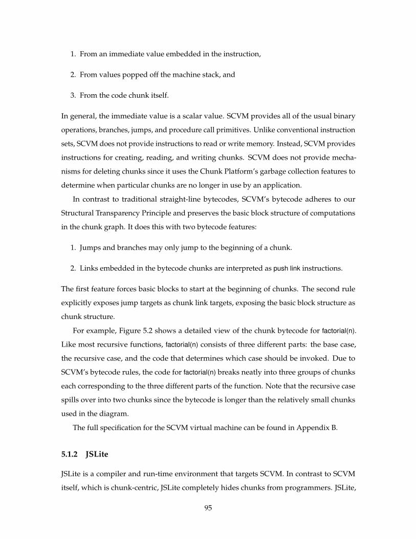
1. From an immediate value embedded in the instruction,

2. From values popped off the machine stack, and

3. From the code chunk itself.

In general, the immediate value is a scalar value. SCVM provides all of the usual binary

operations, branches, jumps, and procedure call primitives. Unlike conventional instruction

sets, SCVM does not provide instructions to read or write memory. Instead, SCVM provides

instructions for creating, reading, and writing chunks. SCVM does not provide mecha-

nisms for deleting chunks since it uses the Chunk Platform’s garbage collection features to

determine when particular chunks are no longer in use by an application.

In contrast to traditional straight-line bytecodes, SCVM’s bytecode adheres to our

Structural Transparency Principle and preserves the basic block structure of computations

in the chunk graph. It does this with two bytecode features:

1. Jumps and branches may only jump to the beginning of a chunk.

2. Links embedded in the bytecode chunks are interpreted as push link instructions.

The first feature forces basic blocks to start at the beginning of chunks. The second rule

explicitly exposes jump targets as chunk link targets, exposing the basic block structure as

chunk structure.

For example, Figure 5.2 shows a detailed view of the chunk bytecode for factorial(n).

Like most recursive functions, factorial(n) consists of three different parts: the base case,

the recursive case, and the code that determines which case should be invoked. Due to

SCVM’s bytecode rules, the code for factorial(n) breaks neatly into three groups of chunks

each corresponding to the three different parts of the function. Note that the recursive case

spills over into two chunks since the bytecode is longer than the relatively small chunks

used in the diagram.

The full specification for the SCVM virtual machine can be found in Appendix B.

5.1.2 JSLite

JSLite is a compiler and run-time environment that targets SCVM. In contrast to SCVM

itself, which is chunk-centric, JSLite completely hides chunks from programmers. JSLite,

95

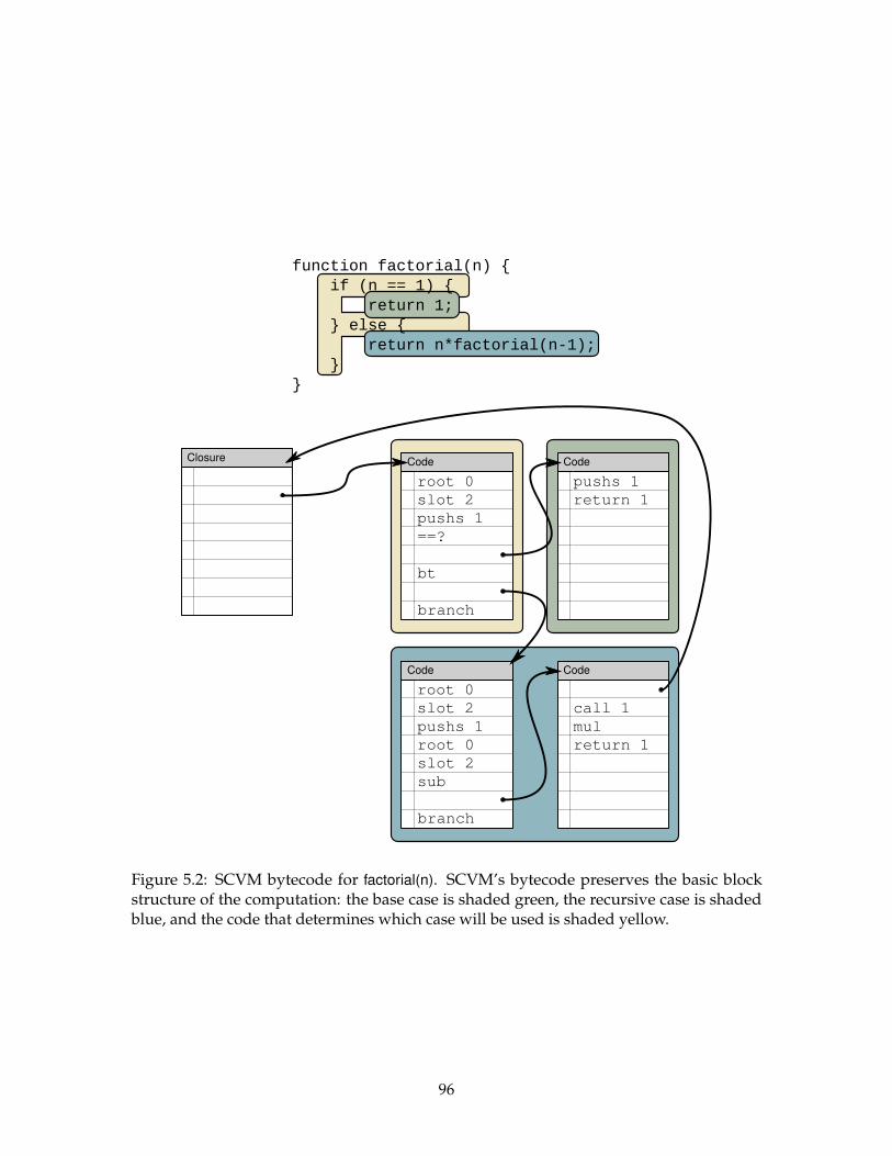
ClosureCode

CodeCode

pushs 1

root 0

slot 2

==?

bt

branch

pushs 1

root 0

slot 2

root 0

slot 2

sub

branch

mul

call 1

return 1

CodeClosure

function factorial(n) {

if (n == 1) {

return 1;

} else {

return n*factorial(n-1);

}

}

pushs 1

return 1

Figure 5.2: SCVM bytecode for factorial(n). SCVM’s bytecode preserves the basic blockstructure of the computation: the base case is shaded green, the recursive case is shadedblue, and the code that determines which case will be used is shaded yellow.

96

by providing a familiar language and set of libraries that make use of chunks and chunk

features without showing that the underlying implementation is in chunks, indicates that

the Chunk Model can be used for general-purpose computing tasks without requiring the

end-user programmer to understand whole chunk computing model.

JSLite is a subset of the JavaScript language. Like JavaScript, JSLite is a scoped, closure-

based language. The JSLite programming model fits well with the environment-based

model exposed by SCVM. JSLite includes a standard library that implements the primitive

JavaScript types, including arrays, strings, and objects. The standard library is chunk-aware

and provides reasonably fast, variable-sized objects in the face of fixed-sized chunks and

loss of random access memory. For example, the Array implementation provides O(log(n))

worst-case random indexing with fast appends by gradually building n-ary search trees for

elements as those elements are appended.

The JSLite compiler and standard library make full use of the Chunk Platform’s facilities.

For example, rather than implementing its own garbage collector, JSLite leverages the

distributed garbage collector of the Chunk Peer to garbage collect objects as they fall into

disuse. JSLite programs can make use of multiple SCVM interpreters running on multiple

Chunk Runtimes to provide a parallel shared memory programming environment; this

functionality relies heavily on the shared-chunk primitives exposed by the Chunk API.

To aid programmers in the shared memory environment, JSLite’s standard library

includes the parallel library. The parallel library implements a selection of parallelism

primitives that enable JSLite computations to spawn new threads of computation on other

nodes and synchronize with those threads. For example, the spawn(fn, args...) spawns a

computation on another node, while the parallel.Barrier prototype object provides a simple

synchronization barrier.

Appendix C contains big_jacobi.js, a JSLite-based implementation of the Jacobi relaxation

method of solving a system of linear equations. As we co-developed the JSLite compiler,

SCVM, and big_jacobi.js, we attempted to push as much complexity as possible away

from the programmer. As a result, big_jacobi.js is a straight-forward implementation of

Jacobi relaxation that uses nested Arrays for matrices and barriers for synchronization

and that requires no Chunk Platform-specific workarounds. The Jacobi program stresses

the entire Chunk Platform, especially the Chunk Exchange Protocol, since it makes heavy

97

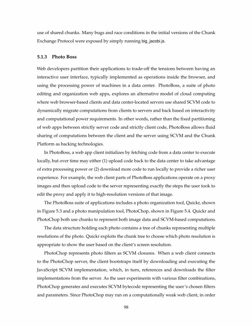
use of shared chunks. Many bugs and race conditions in the initial versions of the Chunk

Exchange Protocol were exposed by simply running big_jacobi.js.

5.1.3 Photo Boss

Web developers partition their applications to trade-off the tensions between having an

interactive user interface, typically implemented as operations inside the browser, and

using the processing power of machines in a data center. PhotoBoss, a suite of photo

editing and organization web apps, explores an alternative model of cloud computing

where web browser-based clients and data center-located servers use shared SCVM code to

dynamically migrate computations from clients to servers and back based on interactivity

and computational power requirements. In other words, rather than the fixed partitioning

of web apps between strictly server code and strictly client code, PhotoBoss allows fluid

sharing of computations between the client and the server using SCVM and the Chunk

Platform as backing technologies.

In PhotoBoss, a web app client initializes by fetching code from a data center to execute

locally, but over time may either (1) upload code back to the data center to take advantage

of extra processing power or (2) download more code to run locally to provide a richer user

experience. For example, the web client parts of PhotoBoss applications operate on a proxy

images and then upload code to the server representing exactly the steps the user took to

edit the proxy and apply it to high-resolution versions of that image.

The PhotoBoss suite of applications includes a photo organization tool, Quickr, shown

in Figure 5.3 and a photo manipulation tool, PhotoChop, shown in Figure 5.4. Quickr and

PhotoChop both use chunks to represent both image data and SCVM-based computations.

The data structure holding each photo contains a tree of chunks representing multiple

resolutions of the photo. Quickr exploits the chunk tree to choose which photo resolution is

appropriate to show the user based on the client’s screen resolution.

PhotoChop represents photo filters as SCVM closures. When a web client connects

to the PhotoChop server, the client bootstraps itself by downloading and executing the

JavaScript SCVM implementation, which, in turn, references and downloads the filter

implementations from the server. As the user experiments with various filter combinations,

PhotoChop generates and executes SCVM bytecode representing the user’s chosen filters

and parameters. Since PhotoChop may run on a computationally weak web client, in order

98

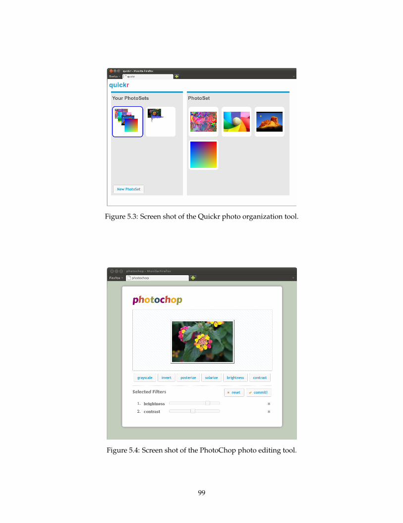
Figure 5.3: Screen shot of the Quickr photo organization tool.

Figure 5.4: Screen shot of the PhotoChop photo editing tool.

99

to enable interactive experimentation with filters, PhotoChop normally only operates on

small resolution versions of photos. When the user finishes her experimentation, Photo-

Chop generates “final” SCVM bytecode to apply the filters to all resolutions of the photo.

Normally, the web browser chooses to migrate the code to a fast remote server to operate

on the high resolution photos, but depending on communication costs, PhotoChop may opt

to run all of the bytecode locally, or split computation between local and remote servers.

5.2 Tasklets

Currently, there are two popular models for selling and accounting for use of cloud comput-

ing resources: (1) charging per usage hour for generic virtual machines, e.g., as in Amazon

EC2 [8] and Windows Azure [70], and (2) charging for fine-grained service requests, e.g.,

as in Google App Engine [42]. While the virtual machine approach offers maximum flex-

ibility with respect to the programming model, coarse-grained accounting restricts the

kinds of jobs that may run. Because virtual machines require significant initial setup, they

are best suited for large numbers of identical tasks that (1) may be combined to amortize

machine setup and maintenance, and (2) may consume every rented minute of computa-

tion, as unused capacity goes to waste. In contrast, the fine-grained accounting model of

Google App Engine enables small tasks to take up only small amounts of rented time, but

requires the programmer to structure her application around the particular fine-grained

request/response interfaces of Google App Engine.

The PhotoBoss application of the previous section hints at another model for cloud

computing: trading the execution of small tasks between clients with tasks to perform

and servers that may perform those tasks for a price. The core enabler of this new cloud

programming model is the Tasklet. A Tasklet is an SCVM Thread packaged with metadata

concerning the cost and performance requirements of the task. Tasklets are supported by

Tasklet Containers that may execute Tasklets in a local SCVM interpreter as well as offload

Tasklets to third-party Tasklet Containers running on other hosts. Tasklet Containers

may run as new cloud services (e.g., Tasklets as a Service), in idle time on top of existing

cloud services (e.g., as a process that takes up the remaining slack time on an already

running Amazon EC2 instance), or in idle time on locally available computing hardware

(e.g., as in resource foraging systems). Since SCVM structures are self-contained, it is

100

possible to migrate a computation between Tasklet Containers by pausing the computation,

shipping the Tasklet’s chunks to the remote Container, and resuming computation with

the transferred chunks. In contrast to a virtual machine that needs to be appropriately

configured before use, all Tasklet Containers are “blank slates” that rely on a Tasklet linking

to all of the data and libraries that it needs in order to execute.

Tasklets enable generic computation at fine-grained scales. Compared to the Amazon

EC2 virtual machine model, the Tasklet model allows clients to offload relatively small

tasks. Compared to the Google App Engine model, the Tasklet model is application-generic

and gives the programmer more flexibility in choice of programming frameworks. Thus,

Tasklets fill the gap between request-based models and virtual machine-based models.

5.2.1 Tasklet Accounting with Chunks

Proper accounting for resource usage is crucial when building a system that charges for the

execution of tasks. The fixed-size nature of chunks enables the Tasklet layer to account for

resource usage by counting chunks. For example, bandwidth consumption is measured as

the number of chunks transferred between two hosts while computation consumption is

measured as the number of chunks executed. While it is possible to account for resource

consumption using multiple different metrics, e.g., bytes for network transfers and millisec-

onds for compute time, using a single unit to measure resource usage makes it easier to

build an economy since there is only one currency to trade.

The chunk-based foundation for Tasklets encourages fine-grained accounting by en-

couraging the use of fine-grained, chunk-based data structures. Similarly, the fined-grained

nature of Tasklets enables us to make use of large libraries (e.g, for image filtering or speech

recognition) or large data sets, but only transfer the specific parts of the libraries or data

sets necessary to complete the Tasklet’s particular computation.

While recording run-time usage is important for simple accounting, a client may wish

to predict costs before making a decision to offload a Tasklet to a particular Container.

Static analysis or Tasklet execution history can help predict how much computing time

is required to compute a Tasklet. For example, for the factorial(n) function illustrated in

Figure 5.2, a static analyzer can determine an exact solution for the number of chunks

executed. The factorial(n) function executes two chunks for the base case of n = 1 and

three chunks for n > 1, leading to a closed form execution time of 3(n − 1) + 2 chunks.

101

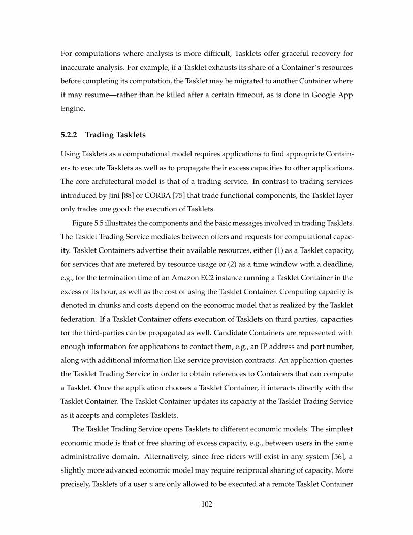
For computations where analysis is more difficult, Tasklets offer graceful recovery for

inaccurate analysis. For example, if a Tasklet exhausts its share of a Container’s resources

before completing its computation, the Tasklet may be migrated to another Container where

it may resume—rather than be killed after a certain timeout, as is done in Google App

Engine.

5.2.2 Trading Tasklets

Using Tasklets as a computational model requires applications to find appropriate Contain-

ers to execute Tasklets as well as to propagate their excess capacities to other applications.

The core architectural model is that of a trading service. In contrast to trading services

introduced by Jini [88] or CORBA [75] that trade functional components, the Tasklet layer

only trades one good: the execution of Tasklets.

Figure 5.5 illustrates the components and the basic messages involved in trading Tasklets.

The Tasklet Trading Service mediates between offers and requests for computational capac-

ity. Tasklet Containers advertise their available resources, either (1) as a Tasklet capacity,

for services that are metered by resource usage or (2) as a time window with a deadline,

e.g., for the termination time of an Amazon EC2 instance running a Tasklet Container in the

excess of its hour, as well as the cost of using the Tasklet Container. Computing capacity is

denoted in chunks and costs depend on the economic model that is realized by the Tasklet

federation. If a Tasklet Container offers execution of Tasklets on third parties, capacities

for the third-parties can be propagated as well. Candidate Containers are represented with

enough information for applications to contact them, e.g., an IP address and port number,

along with additional information like service provision contracts. An application queries

the Tasklet Trading Service in order to obtain references to Containers that can compute

a Tasklet. Once the application chooses a Tasklet Container, it interacts directly with the

Tasklet Container. The Tasklet Container updates its capacity at the Tasklet Trading Service

as it accepts and completes Tasklets.

The Tasklet Trading Service opens Tasklets to different economic models. The simplest

economic mode is that of free sharing of excess capacity, e.g., between users in the same

administrative domain. Alternatively, since free-riders will exist in any system [56], a

slightly more advanced economic model may require reciprocal sharing of capacity. More

precisely, Tasklets of a user u are only allowed to be executed at a remote Tasklet Container

102

Tasklet Container

Thread

Env

Closure

Code"root 0"

"slot 2"

"pushs 1"

"==?"

"bt"

"branch"

Code"pushs 1"

"return 1"

Code"root 0"

"slot 2"

"pushs 1"

"root 0"

"sub"

"branch"

"slot 2"

Env

"4"

"3"

Code

"call 1"

"mul"

"return 1"

"root 1"

Thread

Env

Closure

Code"root 0"

"slot 2"

"pushs 1"

"==?"

"bt"

"branch"

Code"pushs 1"

"return 1"

Code"root 0"

"slot 2"

"pushs 1"

"root 0"

"sub"

"branch"

"slot 2"

Env

"4"

"3"

Code

"call 1"

"mul"

"return 1"

"root 1"

1. register_capacity

5. update

Tasklet TradingService

3. candidates

2. request_capacity

Applications(Tasklets for Execution)

4. executeCode

pushs 2

root 0

slot 2

mul

return 1

Environment

2

Environment

"environ"

42

715

Thread

PC Slot#

Closure

Code

pushs 2

root 0

slot 2

mul

return 1

Environment

2

Environment

"environ"

42

715

Thread

PC Slot#

Closure

Code

pushs 2

root 0

slot 2

mul

return 1

Environment

2

Environment

"environ"

42

715

Thread

PC Slot#

Closure

Code

pushs 2

root 0

slot 2

mul

return 1

Environment

2

Environment

"environ"

42

715

Thread

PC Slot#

Closure

Figure 5.5: Tasklet Trading Service

if the ratio between the Tasklets that u’s Container has executed on behalf of other users,

o, and the Tasklets that u has remotely executed, r, is greater than a threshold, t. In other

words, if o/r > t holds the user may execute Tasklets with other users’ Containers. Lastly,

the Tasklet Trading Service may operate using currency, both virtual or real. It is unclear

what the best Tasklet economic model is; it is fertile ground for future work.

5.3 ChunkStream

The ChunkStream video system implements a video playback library using the ChunkStream

data structure of Section 2.3.1. While the general ideas behind the ChunkStream structure

remain the same, in order to build a real system, two adjustments had to be made to it to

handle real video streams. First, the ChunkStream system augments the FrameData chunks

with additional information to handle non-linear inter-frame dependencies in video codecs.

Second, since most video clips include other streams of data, the ChunkStream system adds

non-video streams to the ChunkStream data structure.

5.3.1 Codec Considerations

In traditional video files, raw data is organized according to a container format such as

MPEG-TS, MPEG-PS, MP4, or AVI. ChunkStream’s IndexTrees, backbones, and Lane-

Markers serve to organize raw encoded streams and, as such, may be considered to be a

chunk-based container format.

Container formats offer many advantages over raw codec streams. Most formats allow

a single file to contain multiple streams, such as a video stream and one or more audio

103

streams, as well as provide different features depending on the environment. Some formats,

like MPEG-TS, include synchronization markers that require more bandwidth, but tolerate

packet loss or corruption, while others are optimized for more reliable, random-access

media. However, at its core, the job of the container format is to present encoded data in

the order in which the decoder needs it.

This is especially important for video codecs that use inter-frame compression tech-

niques because properly decoding a particular frame may depend on properly decoding

other frames in the stream. For example, the H.264 codec [2] includes intra frames (I-frames)

that can be decoded independently of any other frame; predictive frames (P-frames) that

depend on the previously displayed I- or P-frames; and bi-predictive frames (B-frames) that

depend on not only the previously displayed I- or P-frames, but also the next I- or P-frames

to be displayed. P-frames are useful when only a small part of the picture changes between

frames, for example, in a clip of a talking head. B-frames are useful when picture data is

needed for the current frame is available from later frames in the clip, e.g., in a clip where a

camera pans across a landscape or background scenery flows past a moving vehicle.

An H.264 stream that is encoded using P- and B-frames is substantially smaller at the

same quality level than a stream encoded using only I-frames. Unfortunately for video

players, using inter-frame compression complicates seeking, high-speed playback, and

other non-linear operations because frames are no longer independent and instead must be

considered in the context of other frames. For example, a client that seeks to a P- or B-frame

and displays only that frame without fetching other frames in its context will either not be

able to decode the frame or decode a distorted image. Moreover, in codecs like H.264 with

bi-predictive frames, the order in which frames are decoded is decoupled from the order

in which frames are displayed, and the container must ensure that the decoder gets all the

data it needs (including out-of-order frames) in order to decode the current frame. In other

words, a container format contains the raw encoded streams in “decode order” rather than

display or “presentation order”.

Frames in a ChunkStream backbone are always in presentation order. ChunkStream uses

presentation order because each lane in a stream may be encoded with different parameters

or even different codecs, potentially forcing each lane to have a different decode order. To

help clients determine the frame decode order, ChunkStream augments the FrameData

104

Backbone

LaneMarkers

Lane

FrameContext

Frame #1(I-frame)

Frame #2(P-frame)

Frame #4(P-frame)

Frame #3(B-frame)

Figure 5.6: FrameContext chunks allow inter-frame compression by exposing the depen-dencies of a particular frame. The first slot in the FrameContext chunk always points to theI-frame that serves as the foundation of the dependent group of pictures and subsequentslots point to frames in the dependency chain between the I-frame and the current frame inthe required decode order.

chunks that make up each lane with FrameContext chunks that specify the dependencies of

each frame.

Each FrameContext chunk contains a link to each FrameData chunk that the frame

depends on, one link per chunk slot, in the order that the frames must be decoded. Frame-

Context chunks contain the full context for each frame, so that the frame can be decoded

without consulting any other frame’s FrameContext chunks. As a consequence, the first

slot of a FrameContext chunk always points to the previous I-frame in presentation order.

For example, Figure 5.6 shows a portion of an H.264-encoded video clip using inter-

frame compression. Since I-frames can be decoded independently, frame 1 has no Frame-

Context chunk. Frame 2 is a P-frame, and as such, depends on frame 1. Frame 2, therefore,

has a FrameContext chunk that specifies that frame 1 must be decoded before frame 2 can

be decoded. Similarly, frame 4 has a FrameContext chunk that specifies that frame 2, and as

a consequence, frame 1 must be decoded before it can be decoded1. Finally, frame 3 is a

B-frame and as such depends on both frame 2 and frame 4, and by dependency, frame 1, so

its FrameContext chunk lists frames 1, 2, and 4.

1In order to prevent circular references, H.264 does not allow P-frames to depend on B-frames, but only onprevious P- or I-frames. As such, frame 4 cannot depend on frame 3.

105

5.3.2 Multimedia and Parallel Streams

So far, this thesis has only concentrated only on video streams within the ChunkStream

data structures. However, most “videos” are multi-media and contain more than just

video streams: a typical video file also normally contains at least one audio stream and

occasionally metadata streams like subtitles. These additional streams compliment the

original video and should be played along with the chosen video stream.

More generally, each of the sub-streams of a multimedia stream may be a part of a

parallel stream. ChunkStream represents parallel streams by allowing LaneMarker chunks

to contain lanes from multiple semantic streams. Recall that each lane of a LaneMarker

chunk contains a link to a StreamDescription chunk with a stream identifier as well as a

link to the actual data in that lane. ChunkStream clients use the stream identifier slot of

StreamDescription chunks to determine which lanes are alternate versions of the same

stream (two or more lanes have identical stream identifiers) and which lanes are parallel

streams (two lanes have different stream identifiers).

106

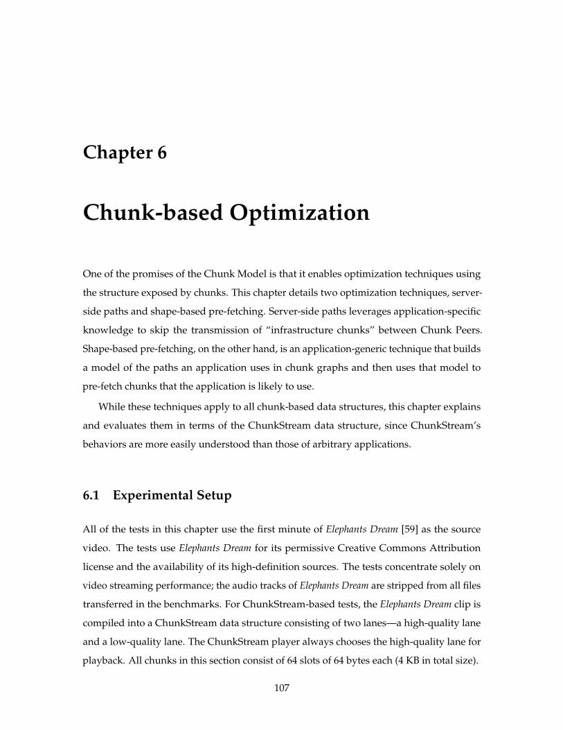
Chapter 6

Chunk-based Optimization

One of the promises of the Chunk Model is that it enables optimization techniques using

the structure exposed by chunks. This chapter details two optimization techniques, server-

side paths and shape-based pre-fetching. Server-side paths leverages application-specific

knowledge to skip the transmission of “infrastructure chunks” between Chunk Peers.

Shape-based pre-fetching, on the other hand, is an application-generic technique that builds

a model of the paths an application uses in chunk graphs and then uses that model to

pre-fetch chunks that the application is likely to use.

While these techniques apply to all chunk-based data structures, this chapter explains

and evaluates them in terms of the ChunkStream data structure, since ChunkStream’s

behaviors are more easily understood than those of arbitrary applications.

6.1 Experimental Setup

All of the tests in this chapter use the first minute of Elephants Dream [59] as the source

video. The tests use Elephants Dream for its permissive Creative Commons Attribution

license and the availability of its high-definition sources. The tests concentrate solely on

video streaming performance; the audio tracks of Elephants Dream are stripped from all files

transferred in the benchmarks. For ChunkStream-based tests, the Elephants Dream clip is

compiled into a ChunkStream data structure consisting of two lanes—a high-quality lane

and a low-quality lane. The ChunkStream player always chooses the high-quality lane for

playback. All chunks in this section consist of 64 slots of 64 bytes each (4 KB in total size).

107

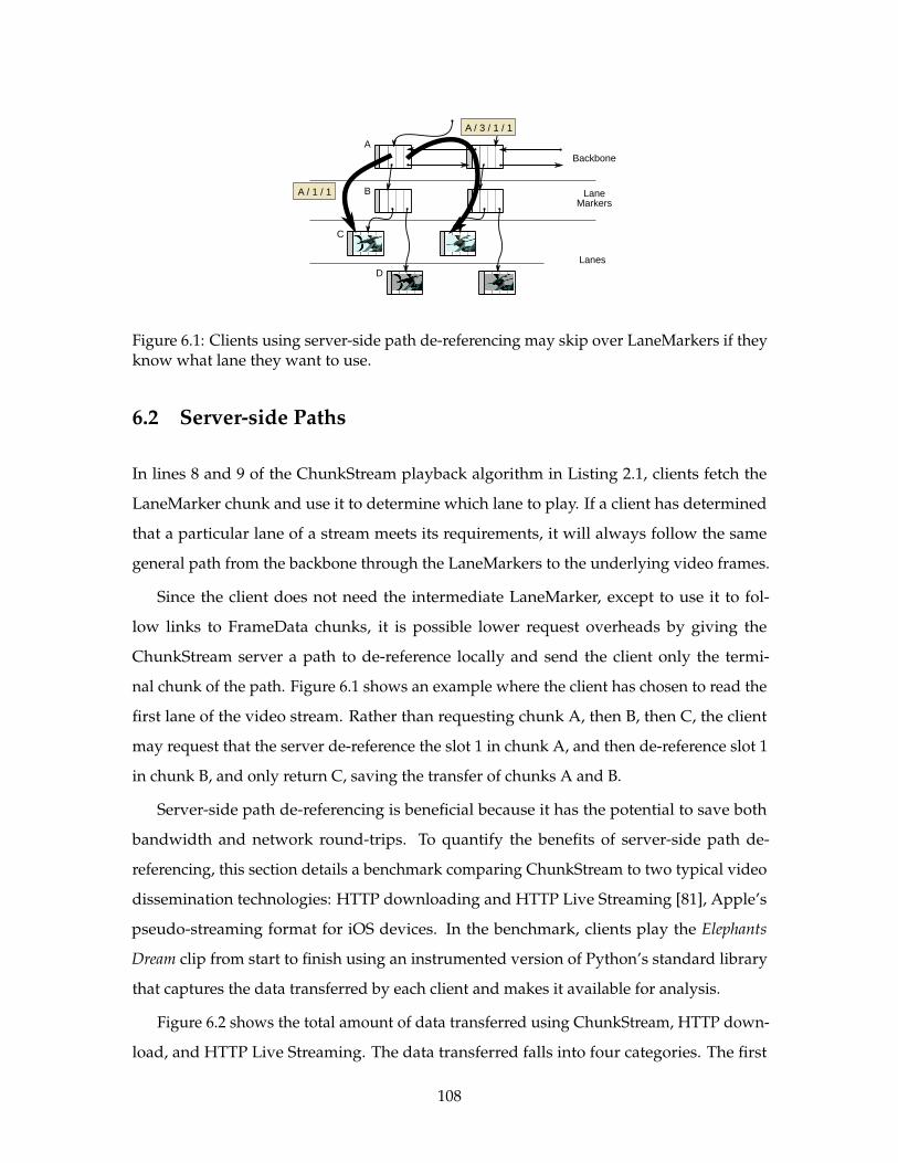
Backbone

Lane

Markers

Lanes

A

B

C

D

A / 1 / 1

A / 3 / 1 / 1

Figure 6.1: Clients using server-side path de-referencing may skip over LaneMarkers if theyknow what lane they want to use.

6.2 Server-side Paths

In lines 8 and 9 of the ChunkStream playback algorithm in Listing 2.1, clients fetch the

LaneMarker chunk and use it to determine which lane to play. If a client has determined

that a particular lane of a stream meets its requirements, it will always follow the same

general path from the backbone through the LaneMarkers to the underlying video frames.

Since the client does not need the intermediate LaneMarker, except to use it to fol-

low links to FrameData chunks, it is possible lower request overheads by giving the

ChunkStream server a path to de-reference locally and send the client only the termi-

nal chunk of the path. Figure 6.1 shows an example where the client has chosen to read the

first lane of the video stream. Rather than requesting chunk A, then B, then C, the client

may request that the server de-reference the slot 1 in chunk A, and then de-reference slot 1

in chunk B, and only return C, saving the transfer of chunks A and B.

Server-side path de-referencing is beneficial because it has the potential to save both

bandwidth and network round-trips. To quantify the benefits of server-side path de-

referencing, this section details a benchmark comparing ChunkStream to two typical video

dissemination technologies: HTTP downloading and HTTP Live Streaming [81], Apple’s

pseudo-streaming format for iOS devices. In the benchmark, clients play the Elephants

Dream clip from start to finish using an instrumented version of Python’s standard library

that captures the data transferred by each client and makes it available for analysis.

Figure 6.2 shows the total amount of data transferred using ChunkStream, HTTP down-

load, and HTTP Live Streaming. The data transferred falls into four categories. The first

108

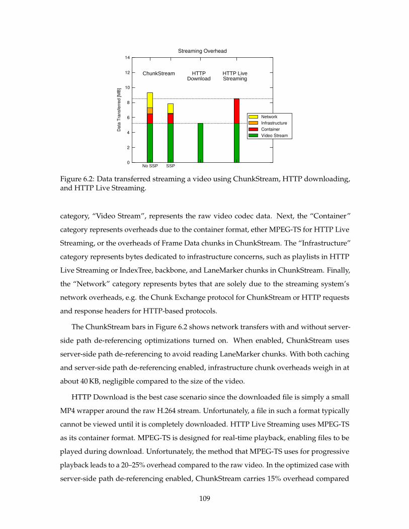
0

2

4

6

8

10

12

14

Da

ta T

ran

sfe

rre

d [

MB

]

Streaming Overhead

ChunkStream

No SSP SSP

Infrastructure

Container

Video Stream

Network

HTTP LiveStreaming

HTTPDownload

Figure 6.2: Data transferred streaming a video using ChunkStream, HTTP downloading,and HTTP Live Streaming.

category, “Video Stream”, represents the raw video codec data. Next, the “Container”

category represents overheads due to the container format, ether MPEG-TS for HTTP Live

Streaming, or the overheads of Frame Data chunks in ChunkStream. The “Infrastructure”

category represents bytes dedicated to infrastructure concerns, such as playlists in HTTP

Live Streaming or IndexTree, backbone, and LaneMarker chunks in ChunkStream. Finally,

the “Network” category represents bytes that are solely due to the streaming system’s

network overheads, e.g. the Chunk Exchange protocol for ChunkStream or HTTP requests

and response headers for HTTP-based protocols.

The ChunkStream bars in Figure 6.2 shows network transfers with and without server-

side path de-referencing optimizations turned on. When enabled, ChunkStream uses

server-side path de-referencing to avoid reading LaneMarker chunks. With both caching

and server-side path de-referencing enabled, infrastructure chunk overheads weigh in at

about 40 KB, negligible compared to the size of the video.

HTTP Download is the best case scenario since the downloaded file is simply a small

MP4 wrapper around the raw H.264 stream. Unfortunately, a file in such a format typically

cannot be viewed until it is completely downloaded. HTTP Live Streaming uses MPEG-TS

as its container format. MPEG-TS is designed for real-time playback, enabling files to be

played during download. Unfortunately, the method that MPEG-TS uses for progressive

playback leads to a 20–25% overhead compared to the raw video. In the optimized case with

server-side path de-referencing enabled, ChunkStream carries 15% overhead compared

109

1 2 4 8 16 32 64

Prefetch Radius

0.0

0.2

0.4

0.6

0.8

1.0

Hit

Rat

e

Hit Rate

Radius Prefetcher

Figure 6.3: Radius Pre-fetching Performance. Note that the independent variable is plottedon a log scale.

to the raw video, which is better than HTTP Live Streaming and acceptable for consumer

applications.

6.3 Chunk Graph Pre-fetching

The rest of this chapter outlines pre-fetching techniques that use the chunk graph to predict

what chunks will be needed. In general-purpose architectures, there are three kinds of

pre-fetching schemes. Address-based pre-fetchers observe the sequence of addresses a

program accesses and attempts to predict future values [76]. Software-based methods

require cooperation of a compiler to add pre-fetching instructions that the processor acts

upon [20]. Finally, thread-based pre-fetchers speculatively execute threads of computation

without waiting for confirmation from the memory system, allowing them predict addresses

based on the actual program [65, 72]. Rather than pre-fetching based on addresses, which

have no semantic value in the Chunk Model, the pre-fetchers in this section try to predict

which paths in the chunk graph will be used and then pre-fetch those paths. In this section,

a get(id) is considered to be a hit if the chunk with the given ID is resident in the node when

the application calls get() so that the get() call can return immediately without blocking.

The simplest pre-fetching algorithm is one that pre-fetches all chunks a certain radius

away from chunks copied to a node. As shown in Figure 6.3, radius-based pre-fetching is

effective, with a near-100% hit rate at large radii. Unfortunately, the high hit rate comes at

the cost of downloading many chunks that are never used. Table 6.1 illustrates the problem.

110

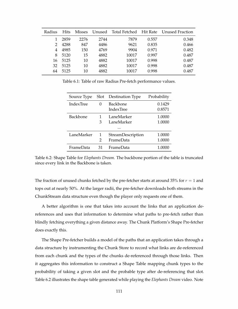
Radius Hits Misses Unused Total Fetched Hit Rate Unused Fraction

1 2859 2276 2744 7879 0.557 0.3482 4288 847 4486 9621 0.835 0.4664 4985 150 4769 9904 0.971 0.4828 5120 15 4882 10017 0.997 0.487

16 5125 10 4882 10017 0.998 0.48732 5125 10 4882 10017 0.998 0.48764 5125 10 4882 10017 0.998 0.487

Table 6.1: Table of raw Radius Pre-fetch performance values.

Source Type Slot Destination Type Probability

IndexTree 0 Backbone 0.1429IndexTree 0.8571

Backbone 1 LaneMarker 1.00003 LaneMarker 1.0000

...

LaneMarker 1 StreamDescription 1.00002 FrameData 1.0000

FrameData 31 FrameData 1.0000

Table 6.2: Shape Table for Elephants Dream. The backbone portion of the table is truncatedsince every link in the Backbone is taken.

The fraction of unused chunks fetched by the pre-fetcher starts at around 35% for r = 1 and

tops out at nearly 50%. At the larger radii, the pre-fetcher downloads both streams in the

ChunkStream data structure even though the player only requests one of them.

A better algorithm is one that takes into account the links that an application de-

references and uses that information to determine what paths to pre-fetch rather than

blindly fetching everything a given distance away. The Chunk Platform’s Shape Pre-fetcher

does exactly this.

The Shape Pre-fetcher builds a model of the paths that an application takes through a

data structure by instrumenting the Chunk Store to record what links are de-referenced

from each chunk and the types of the chunks de-referenced through those links. Then

it aggregates this information to construct a Shape Table mapping chunk types to the

probability of taking a given slot and the probable type after de-referencing that slot.

Table 6.2 illustrates the shape table generated while playing the Elephants Dream video. Note

111

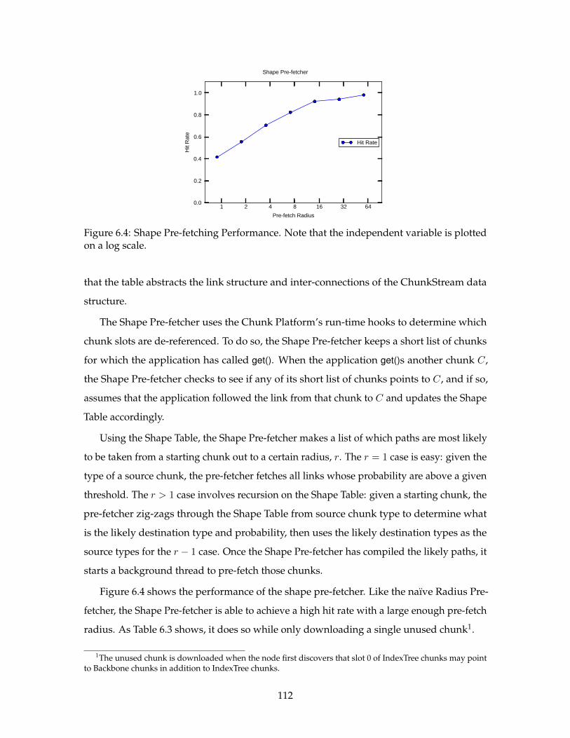
1 2 4 8 16 32 64

Prefetch Radius

0.0

0.2

0.4

0.6

0.8

1.0

Hit

Rat

e

Hit Rate

Shape Prefetcher

Figure 6.4: Shape Pre-fetching Performance. Note that the independent variable is plottedon a log scale.

that the table abstracts the link structure and inter-connections of the ChunkStream data

structure.

The Shape Pre-fetcher uses the Chunk Platform’s run-time hooks to determine which

chunk slots are de-referenced. To do so, the Shape Pre-fetcher keeps a short list of chunks

for which the application has called get(). When the application get()s another chunk C,

the Shape Pre-fetcher checks to see if any of its short list of chunks points to C, and if so,

assumes that the application followed the link from that chunk to C and updates the Shape

Table accordingly.

Using the Shape Table, the Shape Pre-fetcher makes a list of which paths are most likely

to be taken from a starting chunk out to a certain radius, r. The r = 1 case is easy: given the

type of a source chunk, the pre-fetcher fetches all links whose probability are above a given

threshold. The r > 1 case involves recursion on the Shape Table: given a starting chunk, the

pre-fetcher zig-zags through the Shape Table from source chunk type to determine what

is the likely destination type and probability, then uses the likely destination types as the

source types for the r − 1 case. Once the Shape Pre-fetcher has compiled the likely paths, it

starts a background thread to pre-fetch those chunks.

Figure 6.4 shows the performance of the shape pre-fetcher. Like the naïve Radius Pre-

fetcher, the Shape Pre-fetcher is able to achieve a high hit rate with a large enough pre-fetch

radius. As Table 6.3 shows, it does so while only downloading a single unused chunk1.

1The unused chunk is downloaded when the node first discovers that slot 0 of IndexTree chunks may pointto Backbone chunks in addition to IndexTree chunks.

112

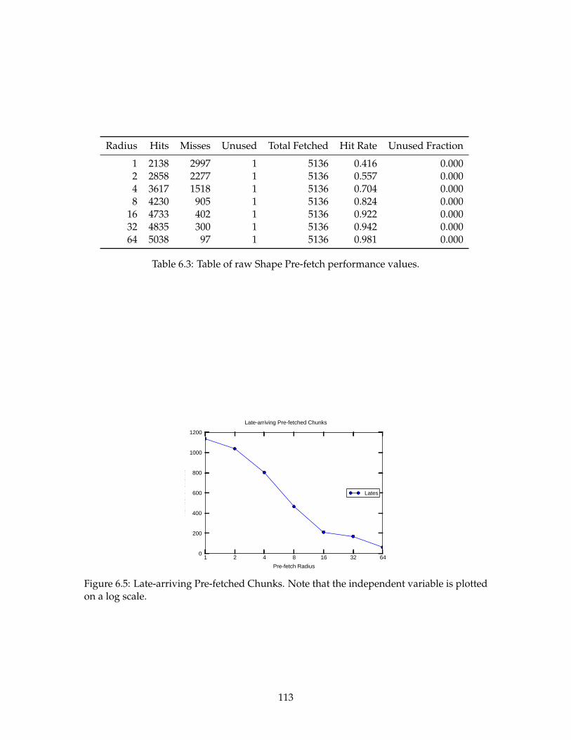
Radius Hits Misses Unused Total Fetched Hit Rate Unused Fraction

1 2138 2997 1 5136 0.416 0.0002 2858 2277 1 5136 0.557 0.0004 3617 1518 1 5136 0.704 0.0008 4230 905 1 5136 0.824 0.000

16 4733 402 1 5136 0.922 0.00032 4835 300 1 5136 0.942 0.00064 5038 97 1 5136 0.981 0.000

Table 6.3: Table of raw Shape Pre-fetch performance values.

1 2 4 8 16 32 64

Prefetch Radius

0

200

400

600

800

1000

1200

Num

ber

of C

hunk

s

Lates

Latearriving Prefetched Chunks

Figure 6.5: Late-arriving Pre-fetched Chunks. Note that the independent variable is plottedon a log scale.

113

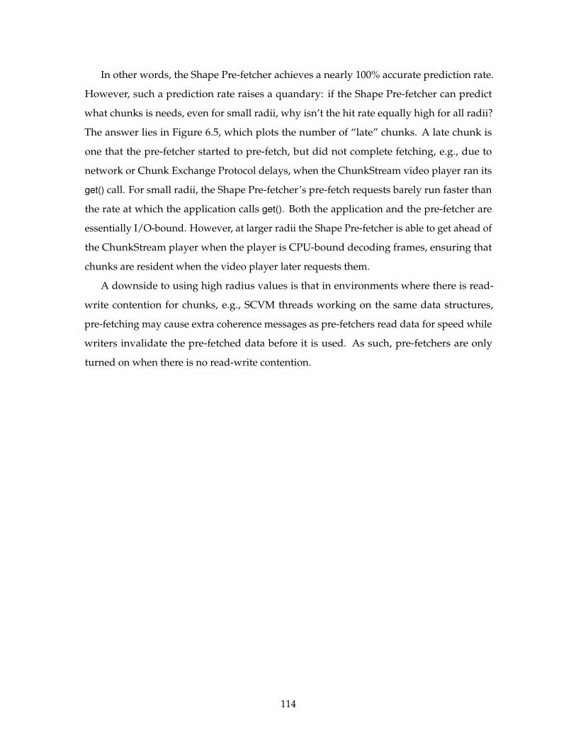
In other words, the Shape Pre-fetcher achieves a nearly 100% accurate prediction rate.

However, such a prediction rate raises a quandary: if the Shape Pre-fetcher can predict

what chunks is needs, even for small radii, why isn’t the hit rate equally high for all radii?

The answer lies in Figure 6.5, which plots the number of “late” chunks. A late chunk is

one that the pre-fetcher started to pre-fetch, but did not complete fetching, e.g., due to

network or Chunk Exchange Protocol delays, when the ChunkStream video player ran its

get() call. For small radii, the Shape Pre-fetcher’s pre-fetch requests barely run faster than

the rate at which the application calls get(). Both the application and the pre-fetcher are

essentially I/O-bound. However, at larger radii the Shape Pre-fetcher is able to get ahead of

the ChunkStream player when the player is CPU-bound decoding frames, ensuring that

chunks are resident when the video player later requests them.

A downside to using high radius values is that in environments where there is read-

write contention for chunks, e.g., SCVM threads working on the same data structures,

pre-fetching may cause extra coherence messages as pre-fetchers read data for speed while

writers invalidate the pre-fetched data before it is used. As such, pre-fetchers are only

turned on when there is no read-write contention.

114

Chapter 7

Related Work

The Chunk Model and Chunk Platform draws from a wealth of related work, spanning

from experimental architectures, operating systems, and mobile systems all the way up to

high-level video streaming protocols and economic models for the cloud.

7.1 Architectures

This thesis is heavily influenced by a series of experimental architectures from the late

1970’s and 1980’s.

The idea of Reference Trees and their many uses for managing objects comes from

Halstead’s doctoral dissertation [47]. In particular, the Chunk Platform’s consistency and

garbage collection strategies are translations of Halstead’s strategies to modern computing

substrates. Halstead uses Reference Trees differently than we do: Halstead’s Reference

Trees protocols provide the functionality of the Chunk Platform’s Channel layer while

independent, higher-level protocols manage object copies and object garbage collection.

In contrast, the Chunk Platform’s Chunk Exchange Protocol is an integrated protocol

that handles the Reference Tree network, chunk consistency, and garbage collection in a

single finite state machine. Our approach requires more state to be kept in Reference Trees

compared to Halstead’s approach, but at the same time provides a more comprehensive

abstraction.

The MuNet [48] machine and corresponding operating environment allowed a compu-

tation to span multiple processors and gradually migrate between them. MuNet inspired

SCVM’s migration techniques.

115

The L project [71] outlines a chunk memory system nearly identical to the Chunk Model

described in this thesis, but with three critical differences. First, L is limited to a fixed

topology of nodes, while the Chunk Platform allows fluid expansion and contraction of

computation nodes. Second, the Chunk Model’s chunks are network-accessible, while L’s

chunks work only in the context of a single machine. Lastly, L uses chunks as the basis for a

new computer architecture, while the Chunk Platform uses chunks as an abstraction above

already existing architectures. These three extensions enable the Chunk Model described in

this thesis to work on the full scale of computers from embedded machines to massively

multi-core machines to clusters of machines.

Ayers’M [9] provides a memory manager for L’s chunks. M provides a single address

space garbage collector as well as techniques for compacting chunks within hardware

virtual memory pages. Many of the techniques inM can be used in a high-performance

implementation of the Chunk Runtime.

A chunk-based system may be able to use optimizations developed for Non-Uniform

Memory Architectures (NUMA). For example, Bolosky et al.’s NUMA kernel [16] uses VM

pages as the unit of sharing and replication. Unfortunately, VM pages are prone to “false

sharing” of different objects on the same VM page. The Chunk Model may suffer from the

same problem if a compiler puts two objects in the same chunk. Fortunately, Granston et

al. [45] argue that the compiler may be able to reduce false sharing by separating objects

into different pages. Chilimbli et al. [23, 24] show that the order of fields in a data structure

may help cache performance; a chunk compiler may re-order slots in a chunk to increase

locality of reference.

7.2 Object Systems and Garbage Collection

The first systems to exploit graph structure of objects and references were the garbage

collection algorithms. Rather than summarize the long history of garbage collection, this

section will briefly outline the key papers that influenced our design of the Chunk Platform’s

garbage collector.

Traditionally, there are two main ways to collect garbage, either reference counting

or tracing. Collectors for LISP introduced tracing and “stop the world” garbage collec-

tion [33, 68]. As address spaces grew, traditional tracing garbage collection became too

116

slow. Bishop [15] created an algorithm that divided memory into independently-collectable

“areas” to reduce garbage collection time. Baker [11] introduced a garbage collector that

(1) bound the costs of garbage collection and (2) spread the costs of garbage collection

across all memory operations, thus removing “long pauses” in the “stop the world” garbage

collectors, enabling garbage collected systems to be used in pseudo-real-time systems.

Later, Hudson et al. [55] introduced a generational garbage collection algorithm based

on the observation that new objects are likely to die, and need to be garbage collected,

more often than older objects. Their “train and car” algorithm divides the address spaces

into independent areas based on the age of objects and then uses a Baker-like real-time

algorithm to garbage collect each area. New areas are garbage collected more frequently

than areas containing older objects. Bacon et al. [10], motivated by the observation that

all high-performance garbage collection algorithms share characteristics of both reference

counting and tracing, unified reference counting and tracing as dual algorithms that operate

on dead object graphs (reference counting) or live object graphs (tracing). A chunk-based

memory may be able to make use of all of these algorithms for the node-local garbage

collector.

More recently, Hirzel et al. [53, 54] built a garbage collector that partition the object

graph based on connectivity, rather than on age. They find that objects that are close to

each other in the object graph (either through direct or transitive relationships) share many

characteristics like lifetime or deathtime and can be more effectively garbage collected when

garbage collected together. Hirzel’s work provides reinforces the hypothesis that object

connectivity may provide useful optimization hints.

There are a wide variety of distributed resource reclamation schemes, ranging from

distributed versions of sequential algorithms, like Lieberman and Hewitt’s extension [63] of

Bishop’s algorithm, to special-purpose distributed schemes. Abdullahi and Ringwood [5]

provide a survey the field of distributed garbage collection. The Chunk Platform’s garbage

collection Chunk State bits are influenced by Dijkstra et al.’s use of graph coloring in the

on-the-fly garbage collector [31]. Like the Chunk Platform’s Reference Trees, SSP chains [87]

enable decentralized resource management. Unlike Reference Trees, SSP chains can only be

used for reference counting and as such, cannot collect reference loops.

117

7.3 Operating Systems

One of the perennial hot topics in operating system design for the past few decades has

been scaling to bigger and more powerful machines; this thesis continues the trend. The

Tornado [39] shared-memory multi-processor operating system aims to scale by leveraging

locality and minimizing both intentional and false sharing. Tornado does so by partitioning

operating system objects into “clustered” objects that may replicated across cores. Chunks

are a natural extension of clustered objects in Tornado. More recently, Corey [17] provides

three new mechanisms—address ranges, kernel cores, and shares—that allow applications

to control what operating system structures are shared on their behalf. Like two threads in

a chunk-based system, two threads in Corey only share what they need to share; everything

else is private to the individual thread. On clusters, Cellular Disco [44] uses clusters of

virtual machines to adapt commodity operating systems to large-scale NUMA machines. In

contrast, we argue for a fundamental re-thinking of the structure of commodity operating

systems around managing chunks.

In the Chunk Model, chunks serve the purpose that virtual memory pages do for typical

operating system kernels, namely that they abstract resource allocation and placement. The

virtual memory system in the Mach microkernel [95] allows memory objects, like chunks, to

be mapped dynamically by applications. Unlike chunks, however, Mach’s memory objects

are unstructured and of arbitrary size, limiting the analysis that may be performed on

them. Alternatively, the Barrelfish multikernel [13] uses information from explicit message

passing to optimize communication, much as it is possible optimize memory allocation

with chunks.

Internet-scale computing have lead to a resurgence in work on massively data-parallel

problems. Google’s MapReduce [29] structures computations into a “map” stage that

transforms data and a “reduce” stage that gathers data into sets. Microsoft’s Dryad and

DryadLINQ [57,96] provide a more generic cluster programming system based on data-flow

graphs comprised of single-threaded computation nodes connected by communication

channels. The Dryad family of projects is notable for its graph-based techniques that allow

a computation to be optimized at run-time simply by modifying the structure of the graph.

Similar optimizations may apply to the chunk graph.

118

In large-scale mutli-processing systems, there is an opportunity to make use of “space-

sharing” of hardware resources rather than just “time-sharing”. The fos [90] factored

operating system for multi-core systems treats cores as an abundant resource that should

be allocated to particular problems. fos replaces the scheduler with a layout algorithm

that allocates applications and OS services to their own dedicated cores. In order for the

layout algorithm to work, fos requires applications to be divided into very finely-grained

structured mini-servers. The chunk abstraction compliments the structural requirements

that fos imposes because chunks explicitly expose the seams in applications and data

structures.

7.4 Code Offload and Migration

Over the past twenty years, many projects have explored how to balance, offload, and mi-

grate code among disparate hardware resources. Adaptive mobile systems, like Odyssey [74],

Puppeteer [28], and Chroma [12] outline the various ways an application may be decom-

posed in a client/server system. Building upon such systems, Flinn et al. propose [36]

methods for choosing when to offload code. Recent projects like MAUI [27] and Clone-

Cloud [25] concentrate on offloading code from smartphones to cloud servers for execution

speed. Yang et al. [94] analyze CloneCloud’s object graph to reduce the amount of state that

must be transferred during migration. ThinkAir [58] provides a framework for dynamically

offloading parallel and divide-and-conquer parallel algorithms to the cloud. In contrast to

these architecture-specific code offload systems, SCVM and the Chunk Platform enables a

simple, yet generic, form of code offloading.

Fuggetta et al. [38] survey the field of code mobility and classifies code migration

systems by the strength of their mobility, the types of resource binding allowed, and

the particular software architecture that the code migration system needs. According to

Fuggetta’s taxonomy, SCVM provides a “code on demand” strong mobility system.

SCVM may make use of cloudlets [84] to offload computations to local compute re-

sources rather than directly to the cloud. SCVM’s data structures are much lighter-weight

than proposed cloudlet implementation of copying virtual machines between mobile nodes

and cloudlet nodes [92].

119

7.5 Pre-fetching

Most existing pre-fetching systems require pre-computed hints to determine how and what

to fetch ahead of time. For example, hoarding in the SPREE [60] mobile object system uses

a compiler pass to statically determine the “shape” of the objects used (e.g., the object fields

accessed in a program, compared to all of the fields available). SPREE sends the current

program counter and a root object to a server, which responds with the objects that the

client needs to hoard. Transparent Informed Prefetching [83] uses high-level disclosure of

application actions to feed its pre-fetcher. In contrast, the Chunk Platform makes use of the

run-time chunk graph to determine what to pre-fetch.

7.6 Tasklet Economic Models

Tasklets provide an alternative way of consuming and paying for computing resources and,

as such, can make use of the multitude of studies about cloud computing economic models.

One of the refreshing aspects of cloud computing, in contrast to privately-run data

centers, is that operational costs are well-known, documented, and studied. For example,

the CloudCmp Project [62] analyzes four different cloud providers in an attempt to guide

consumers to the correct provider. Cloud auto-scaling [66] enables application operators

automatically expand and contract cloud resources depending on external demand.

Goiri et al. [41] derive profit equations for cloud providers that take into account fixed

private cloud resources (that can be shut down or “insourced”/rented to others) and public

cloud resources used at a specific cost rate. Given certain assumptions on power and costs,

Goiri and co-authors find it better to under-provision fixed resources, use the cloud for

bursts, and then insource when the fixed cluster of nodes is not busy. Briscoe and Marinos

argue for a Community Cloud [18] made out of P2P nodes to avoid “necessary evils” like

vendor lock-in, cloud downtime, and privacy problems. Their work includes an idea of

“community currencies” where nodes trade resources in terms of a fungible currency. A

node may run a surplus, which it can then spend against nodes that run a deficit.

Durkee [32] argues that while the competition between cloud providers may reduce

the cost of cloud computing, cloud computing will never be zero-cost. Cloud vendors

operate in a environment of perfect competition (like cellphone vendors and airlines), so

they have to make their profit by obscuring details (e.g., performance or the guarantees of

120

service-level agreements) or costs (e.g., incoming bandwidth costs). Durkee makes the point

that enterprise systems need more reliability and performance guarantees, and predicts

that we will likely end up with a Cloud 2.0 that gives more value, albeit at a higher unit

cost. Tasklets may be seen as one step towards a Cloud 2.0 charging model.

Mesos [52] enables sharing of data center resources among different frameworks (e.g.,

MPI, Dryad, MapReduce, or Hadoop). Mesos works by offering each toolkit resources and

incentivizes the framework to accept only the resources it needs. Our work may benefit

from the incentive structures that Mesos introduces.

Finally, Google App Engine and Amazon EC2 are expanding offerings from the pure

models mentioned in Section 5.2. EC2 Spot Instances [7] enable users to bid on excess

capacity that would otherwise be wasted by Amazon, providing a way of lowering the cost

of EC2 virtual machines. Similarly, App Engine offers Task Queues [43] for long running

tasks that do not fit in a request/response format. Both offerings speak to the need for

additional cloud computing models, of which Tasklets is one alternative.

7.7 Persistent Programming Systems

Persistent programming systems, of which Cahill [19] provides a large survey, provide a

hybrid model that offers the persistence of storage systems and the computation model of

object-oriented programming languages. The abstractions provided by persistent program-

ming systems resemble our chunk abstraction without the size restrictions. For example,

the Mneme object store [73] is built upon object vectors that contain either data or object

references and are stored in files specified by the programmer. To keep object addresses

short (and allow local applications to use purely local names), an object may only refer

to other objects within a particular file. In order to refer to objects external to the file, a

Mneme object points to a “forwarder object” within the file that is treated specially by the

Mneme runtime. More recently, InterWeaves [89] provides an similar object model based

on Internet URLs. The Chunk Model extends the persistence goals of these systems with

notions of locality and hardware resource management.

121

7.8 Locality-aware Re-structuring

Compiler writers have tried to take advantage of locality to improve program performance.

For example, Gloy et al. [40] outline an algorithm for producing a graph of procedure calls

weighted by how execution may alternate between two procedures. His group used the

graph to place code to avoid cache conflicts. The chunk graph may be annotated with

Gloy’s temporal ordering information to help resource allocation.

Others have worked on cache-aware data placement. Calder et al. [21] introduced

Cache-conscious Data Placement (CCDP), a profile- and compiler-driven technique for

placing data within cache blocks. Chilimbi et al. [23, 24] investigated a four techniques for

decreasing cache conflicts. One technique provides a new memory allocator, ccmalloc, that

takes pointer as an additional argument and uses that pointer as a hint of where to place

the newly allocated memory, e.g., place a child node in a tree close to its parent. In many

ways ccmalloc is a step towards the Chunk Model where explicit links denote locality.

Static pointer analysis [51] at compile time promises to aid optimization. However,

static pointer analysis runs into scalability and scope issues: pointer analysis only works

well when it can run over the entire program, including all of the libraries that the program

may use. As such, analysis problems quickly become intractably large.

7.9 Video Streaming

Video streaming solutions fit into three general categories: streaming, downloading, and

pseudo-streaming [46]. Two common streaming solutions are IETF’s RTP/RTSP suite [85,86]

and Adobe’s RTMP [4]. RTP/RTSP uses a combination of specially “hinted” files, TCP

control streams, and UDP data streams to give users frame-accurate playback over both

live and pre-recorded streams. RTMP is a specialized protocol for streaming Flash-based

audio and video over TCP. Unlike RTP/RTSP, RTMP multiplexes a single TCP connection,

allowing it to more easily pass through firewalls and NATs at the cost of the complexity of

multiplexing and prioritizing sub-streams within the TCP connection. Clients have some

control over the stream and may seek to particular timestamps.

On the other hand, many clients “stream” video by downloading a complete video file

over HTTP. HTTP downloading is simple, but does not allow efficient seeking in content that

has not yet been downloaded, nor can it adapt to varying bandwidth constraints. Pseudo-

122

streaming is an extension of the download model that allows clients to view content as it

is downloaded. Recently, Pantos’s work on HTTP Live Streaming [81] extends the HTTP

pseudo-streaming model by chunking long streams into smaller files that are individually

downloaded. A streaming client first downloads a “playlist” that contains the list of

video segments and how long each segment lasts. The client then streams each segment

individually. The HTTP Live Streaming playlist may contain “variant” streams, allowing a

client to switch to a, e.g., lower bandwidth, stream as conditions warrant. Seeking is still

awkward, as the client must download an entire segment before seeking is possible.

Of the three categories, streaming is the most bandwidth-efficient, but pseudo-streaming

and downloading are the most widely implemented, likely because of implementation

simplicity [46].

123

Chapter 8

Summary and Future Work

This thesis starts with two observations about recent trends in computing. The first obser-

vation is that the traditional machine abstraction of strings of assembly code running in a

flat virtual memory hides important details about the machine from programs and details

about programs from the machine. While hiding and abstracting details can be beneficial,

it can also be harmful if the abstraction no longer fits the problem at hand. This leads to

the second observation: modern computing substrates have new features and properties

that do not fit in the traditional computing abstraction. Modern computing substrates

come with their own machine model extensions because the traditional computing model

does not provide enough information about the internal structures of programs and the

machines that run them to build run-time systems to properly support applications on the

substrate. Programmers that wish to use modern computing substrates must use platform-

specific frameworks to manage these new hardware resources. Rather than learning one

machine model, programmers must now master many machines models, each its own

unique extensions, strengths, and caveats.

The goal of this thesis is to test the hypothesis that preserving and exposing structural

information at the machine level will make it easier to build generic system-level support

for wide classes of applications running on a variety of modern computing substrates. In

order to evaluate that hypothesis, we formalize a structured memory model, the Chunk

Model, and build the Chunk Platform, an implementation of the Chunk Model. The Chunk

Model replaces the traditional flat memory with structure-preserving graphs of fixed-size

chunks. The Chunk Model, since it is just a structured generalization of the unstructured

125

von Neumann memory model, is both application-generic and platform-generic, giving us

exactly the foundation we need to test our hypothesis.

We use the Chunk Platform to test the feasibility of building a real system based on the

Chunk Model. The Chunk Platform demonstrates:

• a chunk-based application programming interface that captures application structure

in graphs of chunks,

• a wire format for sharing graphs of chunks between independent nodes of a comput-

ing substrate,

• the Chunk Exchange Protocol, a distributed network protocol that uses Reference

Trees to implement a programmer-friendly sequentially consistent memory model for

shared graphs of chunks,

• a distributed garbage collection algorithm of chunk graphs that can collect cycles

distributed across independent nodes,

• optimization techniques that use the chunk graph to pre-fetch or omit data as needed

by applications,

• SCVM, a chunk-based virtual machine that captures the basic block structure of

programs as chunk structure in graphs, and

• a reference compiler that targets SCVM and makes use of the advantages of the

Chunk Model, yet provides a familiar programming language and programming

environment that hide the details of chunks from the programmer.

We evaluate the Chunk Platform by building a variety of sample applications in both

traditional areas like scientific computing and video streaming, as well as new areas such

cloud computing and task migration.

Our experience implementing the Chunk Platform and the applications that use it testify

to the claim that the Chunk Model is a plausible way of building a structured computing

system that provides useful functionality for applications and run-time layers. For those

who want to experiment with the Chunk Model for themselves, source code is available

from http://o2s.csail.mit.edu/chunks under a free and open source license.

126

8.1 Future Work

As we developed the Chunk Model and Chunk Platform, we made several design decisions

and assumptions that may bear revisiting.

8.1.1 High Performance Chunk Platform

The Chunk Platform described in this thesis is not focused on high performance. While it

provides a useful vehicle for experimentation with small applications, there many ways

to improve the performance of the Chunk Platform. For example, the internals of the

Chunk Runtime use implementation-convenient, but run-time inefficient, objects and data

structures to represent the Channel Peer and Chunk State objects in the Chunk Exchange

layer. A re-write of the Chunk Runtime that pays careful attention to software efficiency

could pay dividends in building a Chunk Platform that can be used to benchmark the

generic Chunk Model against native substrate-specific programming frameworks.

8.1.2 Reference Tree Reliability

The Chunk Exchange Protocol assumes that substrate networks are reliable in order to

provide its correctness guarantees. In the current iteration of the Chunk Exchange Protocol,

the loss of a node or a channel could lead to the partitioning of Reference Trees at best and

at worst lead to loss of data, if, for example, the node that died held the sole valid copy of

a chunk. More complex versions of the Chunk Exchange Protocol may allow the Chunk

Platform to mitigate problems due to faulty nodes. For example, to heal partitioned Refer-

ence Trees, the Chunk Runtimes on nodes around the partition could flood the substrate

network with discovery messages in an attempt to find the other branches of the Reference

Tree. To solve the problem of lost data, future versions of the Chunk Exchange Protocol

could choose to keep invalid shadow copies of chunks around so that if the loss of the sole

copy of the chunk occurs, the system may roll back to an older version of the chunk.

8.1.3 Migration of Computation

The Chunk Platform optimizes chunk placement by using pre-fetchers that can predict

what chunks applications will need. However, as alluded to in the discussion of volumes

of influence in Section 2.3.2 and the implementation of the PhotoBoss web application in

127

Section 5.1.3, another potential way of achieving high-performing chunk systems is to move

entire computations so that threads are close to the resources that they require.

A key challenge is automating migration without requiring the use of programmer-

provided hints or the help of a centralized component that monitors global knowledge of the

entire program, since neither programmer hints nor centralized components scale well. One

promising approach to automatic migration is to expand the distributed representation of

Reference Trees to include a measure of how long each Reference Tree is, how far messages

must travel in the Reference Tree, and the relative distribution of hostage nodes. The Chunk

Runtime on each node could then monitor the new Reference Tree statistics and attempt to

swap computations with neighboring nodes to minimize one of the measures.

A side benefit of automatic migration is that it allows movable computations to cluster

around immobile resources. For example, if a particular computing substrate includes

heterogeneous nodes with different capabilities, computations that make use of the special

features of one node may cluster around that node, enabling efficient use of those specialized

resources.

8.2 Concluding Remarks

Computer science research often assumes that the von Neumann machine abstraction is the

only machine model worth exploring. While making such an assumption is convenient since

von Neumann machines are cheap and plentiful, doing so ignores the value of exploring

alternative assumptions and models. The Chunk Model and Chunk Platform developed in

this thesis represent a new architecture that generalizes the von Neumann model to solve

the abstraction problems of modern computing substrates. The approach presented in this

thesis is but one of many possible new structured computing models that may help us better

use new machines. While researching non-traditional computing models requires more

initial investment in infrastructure, as the field of computer science continues to mature,

investments in alternative architectures allow us the luxury to reconsider our long-held

assumptions and dream of new abstractions that transcend what we have today.

128

Appendix A

Reactor Transition Pseudo-code

This appendix contains pseudo-code implementations of the Reactor transition functions.

The functions take as a request and a chunk ID as parameters.

Each function terminates with one of two primitives. The finish() primitive indicates that

the request has been fully handled and should be removed from the Request Queue. The

Reactor then moves onto the next request, if there is one. The wait() primitive indicates that

the request has not been fulfilled yet. The Reactor will go to sleep until an external change

wakes it up.

The transition functions may make use of two Channel layer messaging functions:

send_status(dest, msg_type, ...) Send a status message of type msg_type to the channel

named by dest.

maybe_send_request(dest, msg_type, chunk_id, requester) Send a request message of type

msg_type to the channel named by dest that originated from requester only if we have

not already sent that message before while handling the current request.

maybe_send_request() helps suppress duplicate messages on the Reference Tree.

129

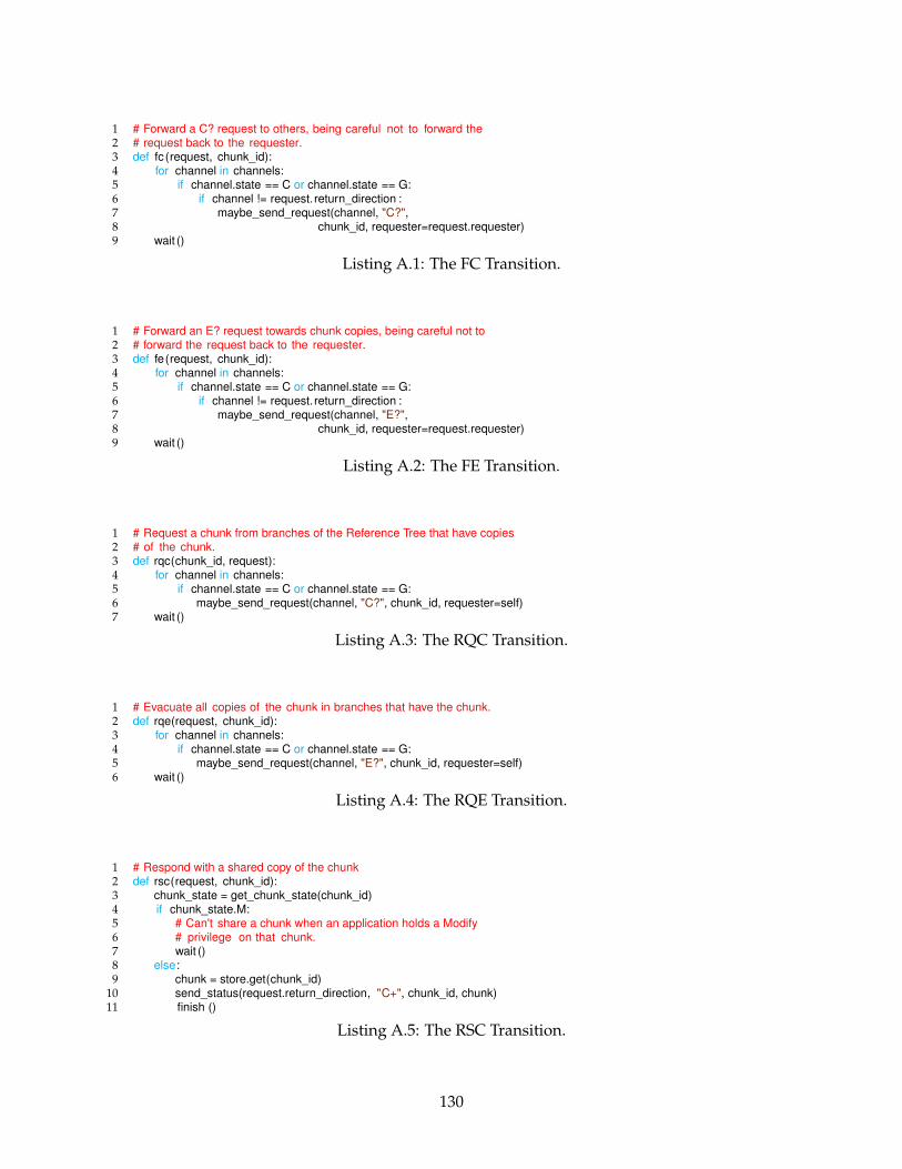
1 # Forward a C? request to others, being careful not to forward the2 # request back to the requester.3 def fc (request, chunk_id):4 for channel in channels:5 if channel.state == C or channel.state == G:6 if channel != request. return_direction :7 maybe_send_request(channel, "C?",8 chunk_id, requester=request.requester)9 wait ()

Listing A.1: The FC Transition.

1 # Forward an E? request towards chunk copies, being careful not to2 # forward the request back to the requester.3 def fe(request, chunk_id):4 for channel in channels:5 if channel.state == C or channel.state == G:6 if channel != request. return_direction :7 maybe_send_request(channel, "E?",8 chunk_id, requester=request.requester)9 wait ()

Listing A.2: The FE Transition.

1 # Request a chunk from branches of the Reference Tree that have copies2 # of the chunk.3 def rqc(chunk_id, request):4 for channel in channels:5 if channel.state == C or channel.state == G:6 maybe_send_request(channel, "C?", chunk_id, requester=self)7 wait ()

Listing A.3: The RQC Transition.

1 # Evacuate all copies of the chunk in branches that have the chunk.2 def rqe(request, chunk_id):3 for channel in channels:4 if channel.state == C or channel.state == G:5 maybe_send_request(channel, "E?", chunk_id, requester=self)6 wait ()

Listing A.4: The RQE Transition.

1 # Respond with a shared copy of the chunk2 def rsc(request, chunk_id):3 chunk_state = get_chunk_state(chunk_id)4 if chunk_state.M:5 # Can't share a chunk when an application holds a Modify6 # privilege on that chunk.7 wait ()8 else:9 chunk = store.get(chunk_id)

10 send_status(request.return_direction, "C+", chunk_id, chunk)11 finish ()

Listing A.5: The RSC Transition.

130

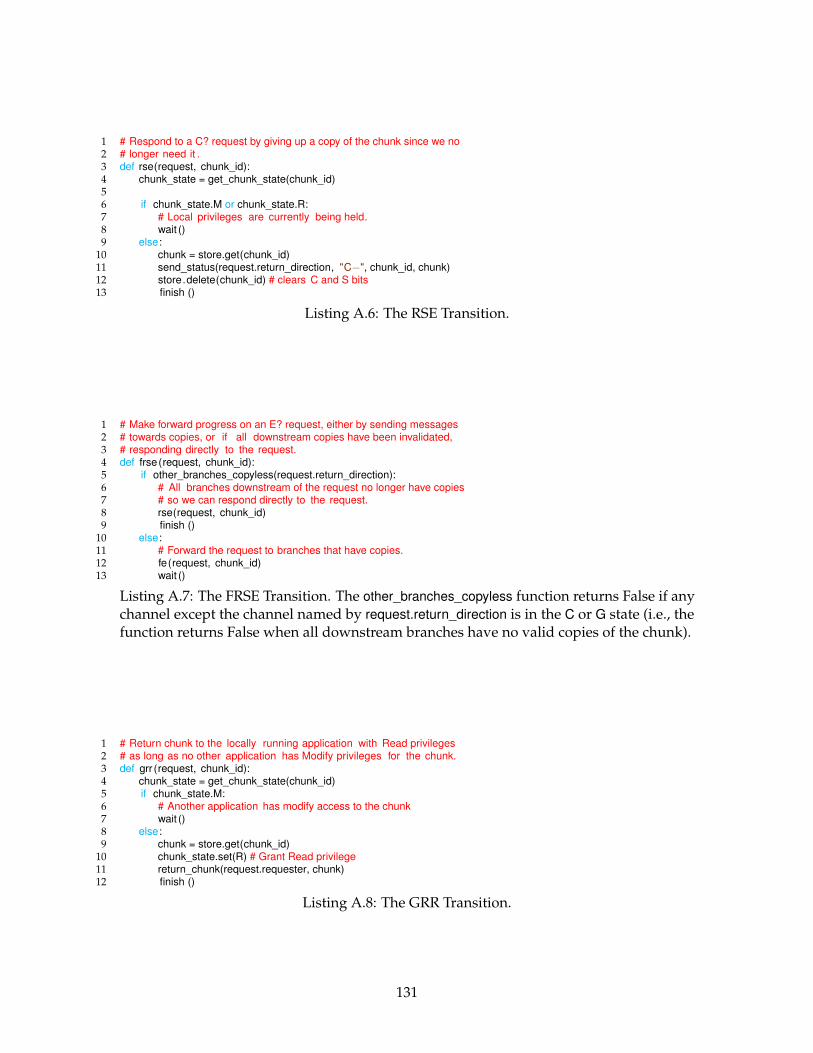
1 # Respond to a C? request by giving up a copy of the chunk since we no2 # longer need it .3 def rse(request, chunk_id):4 chunk_state = get_chunk_state(chunk_id)56 if chunk_state.M or chunk_state.R:7 # Local privileges are currently being held.8 wait ()9 else:

10 chunk = store.get(chunk_id)11 send_status(request.return_direction, "C−", chunk_id, chunk)12 store.delete(chunk_id) # clears C and S bits13 finish ()

Listing A.6: The RSE Transition.

1 # Make forward progress on an E? request, either by sending messages2 # towards copies, or if all downstream copies have been invalidated,3 # responding directly to the request.4 def frse (request, chunk_id):5 if other_branches_copyless(request.return_direction):6 # All branches downstream of the request no longer have copies7 # so we can respond directly to the request.8 rse(request, chunk_id)9 finish ()

10 else:11 # Forward the request to branches that have copies.12 fe(request, chunk_id)13 wait ()

Listing A.7: The FRSE Transition. The other_branches_copyless function returns False if anychannel except the channel named by request.return_direction is in the C or G state (i.e., thefunction returns False when all downstream branches have no valid copies of the chunk).

1 # Return chunk to the locally running application with Read privileges2 # as long as no other application has Modify privileges for the chunk.3 def grr (request, chunk_id):4 chunk_state = get_chunk_state(chunk_id)5 if chunk_state.M:6 # Another application has modify access to the chunk7 wait ()8 else:9 chunk = store.get(chunk_id)

10 chunk_state.set(R) # Grant Read privilege11 return_chunk(request.requester, chunk)12 finish ()

Listing A.8: The GRR Transition.

131

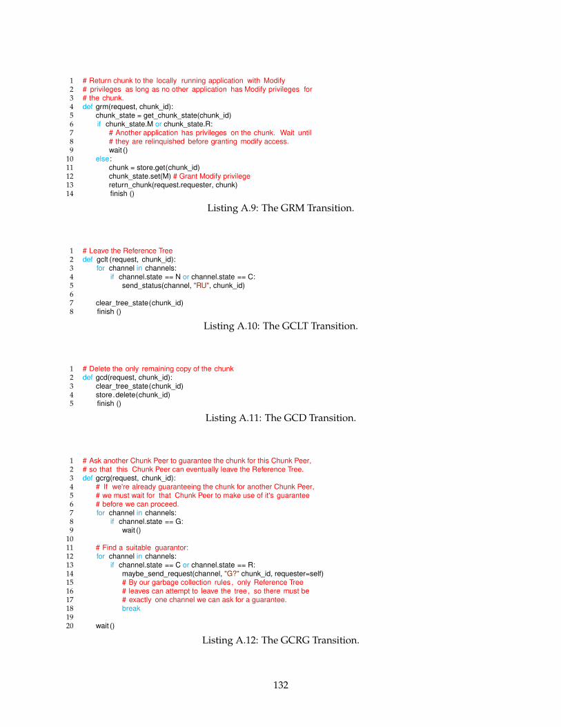
1 # Return chunk to the locally running application with Modify2 # privileges as long as no other application has Modify privileges for3 # the chunk.4 def grm(request, chunk_id):5 chunk_state = get_chunk_state(chunk_id)6 if chunk_state.M or chunk_state.R:7 # Another application has privileges on the chunk. Wait until8 # they are relinquished before granting modify access.9 wait ()

10 else:11 chunk = store.get(chunk_id)12 chunk_state.set(M) # Grant Modify privilege13 return_chunk(request.requester, chunk)14 finish ()

Listing A.9: The GRM Transition.

1 # Leave the Reference Tree2 def gclt (request, chunk_id):3 for channel in channels:4 if channel.state == N or channel.state == C:5 send_status(channel, "RU", chunk_id)67 clear_tree_state(chunk_id)8 finish ()

Listing A.10: The GCLT Transition.

1 # Delete the only remaining copy of the chunk2 def gcd(request, chunk_id):3 clear_tree_state(chunk_id)4 store.delete(chunk_id)5 finish ()

Listing A.11: The GCD Transition.

1 # Ask another Chunk Peer to guarantee the chunk for this Chunk Peer,2 # so that this Chunk Peer can eventually leave the Reference Tree.3 def gcrg(request, chunk_id):4 # If we're already guaranteeing the chunk for another Chunk Peer,5 # we must wait for that Chunk Peer to make use of it's guarantee6 # before we can proceed.7 for channel in channels:8 if channel.state == G:9 wait ()

1011 # Find a suitable guarantor:12 for channel in channels:13 if channel.state == C or channel.state == R:14 maybe_send_request(channel, "G?" chunk_id, requester=self)15 # By our garbage collection rules , only Reference Tree16 # leaves can attempt to leave the tree , so there must be17 # exactly one channel we can ask for a guarantee.18 break1920 wait ()

Listing A.12: The GCRG Transition.

132

Appendix B

SCVM Specification

SVCM is a stack-based, chunk-oriented virtual machine. This makes it different in structure

than most real machines, though it shares some characteristics with other virtual machines

(like Java’s object-oriented VM or Python’s stack-based VM).

SCVM is a stack-based virtual machine. In contrast to a register-based machine that

exposes registers to store ephemeral values, a stack-based machine exposes a stack of values.

Instructions in a stack-based machine manipulate the stack by popping values off the stack,

operating on the values, and pushing values back onto the stack.

SCVM is a chunk-oriented virtual machine. In contrast to a flat-memory machine,

“system memory” is not an individually-addressable array of bytes, but rather a universe

of chunks. SCVM distinguishes between scalar values and references to chunks; it is not

possible to de-reference a scalar value to get a chunk.

B.1 SCVM Programming Environment

SCVM exports an environment- and closure-based computation model. In an environment-

based computation model all data accessible to the computation are accessible through

a linked list of “environments”. Each environment is represented by an Environment

chunk. Programs find, read, and write data by finding the appropriate slots in Environment

chunks. In a closure-based computation model, every function is “closed” in a particular

lexical environment to create a closure. The only way to apply the function is to create

a new environment for the function execution and connect that new environment to the

environment of the closure.

133

B.1.1 Threads

Every thread of computation in SCVM is represented by a Thread chunk. The thread chunk

exposes two slots to the programmer:

Slot 0 Link to environment chunk

Slot 1 Link to the currently executing closure

Slot 0 provides the programmer with access to the environment, and as such, “main

memory”. Slot 1 points to the currently executing closure, allowing programs to easily

make recursive calls.

The rest of the slots in the Thread chunk are implementation specific. In the Python

implementation, the rest of the slots are:

Slot 2 Program counter link to code chunk

Slot 3 Program counter scalar code offset

Slot 4 Link to top of stack

Slot 5 Link to previous thread chunk

The Python implementation uses a new Thread chunk for each function call; other imple-

mentations need not follow this convention.

B.1.2 Environments

Environments are represented using Environment chunks. Environment chunks have the

following format:

Slot 0 Link to parent environment

Slot 1 Link to symbols or empty

Slots 2–(N-1) bound variables

The first slot of the “global environment” Environment chunk is empty; all other Environ-

ment chunks must have a valid parent link. If the Environment has values that may be

looked up by name, the names are defined in a chunk pointed to by slot 1. The format of

the “symbols” chunk is currently undefined. The rest of the slots are bound variables, each

accessed by slot number.

134

B.1.3 Closures and Functions

Closures are represented using Closure chunks. Closure chunks have two defined slots:

Slot 0 link to enclosing environment

Slot 1 link to available functions.

The first slot points to an Environment chunk, while the second slot points to a Function

chunk containing pointers to available implementations of the closed function.

Function chunks have the form:

Slot 2i description of implementation i

Slot 2i+1 link to code chunk

The description is a scalar string. All SCVM interpreters must support SCVM bytecode

with the description scvm and a link to Code chunks. SCVM interpreters may support other

code types each with their own specification for how the code should be called.

Function calls are made by “applying” a closure to a set of arguments. Before the call

to some closure C, the caller pushes the arguments of C on the stack in reverse order (so

that the first argument is at the top of the stack), pushes the a link to the closure, then calls

the function using the call instruction. When interpreting the call instruction, the machine

creates a new Environment chunk E for the function call and set’s E’s parent to be the value

of C’s static environment. The machine then copies the arguments to E as the first N bound

variables. The machine then creates a new Thread chunk T whose environment is E and

whose closure is C. T also contains any necessary information to allow the closure to return

to the caller. Finally, the machine replaces the old Thread chunk with T and starts executing

C’s code. When C returns, any returned values are pushed on to the stack, the caller’s

Thread chunk is restored, and E and T are de-referenced (allowing the Chunk Platform’s

garbage collector to reclaim them as necessary).

Interpreters that support non-SCVM code must use the same calling convention: argu-

ments are pushed on the stack before the call instruction, arguments are popped off during

the call instruction, and all returned values are pushed on the stack when the call instruction

returns.

135

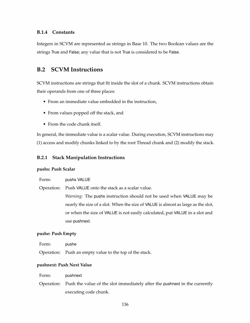
B.1.4 Constants

Integers in SCVM are represented as strings in Base 10. The two Boolean values are the

strings True and False; any value that is not True is considered to be False.

B.2 SCVM Instructions

SCVM instructions are strings that fit inside the slot of a chunk. SCVM instructions obtain

their operands from one of three places:

• From an immediate value embedded in the instruction,

• From values popped off the stack, and

• From the code chunk itself.

In general, the immediate value is a scalar value. During execution, SCVM instructions may

(1) access and modify chunks linked to by the root Thread chunk and (2) modify the stack.

B.2.1 Stack Manipulation Instructions

pushs: Push Scalar

Form: pushs VALUE

Operation: Push VALUE onto the stack as a scalar value.

Warning: The pushs instruction should not be used when VALUE may be

nearly the size of a slot. When the size of VALUE is almost as large as the slot,

or when the size of VALUE is not easily calculated, put VALUE in a slot and

use pushnext.

pushe: Push Empty

Form: pushe

Operation: Push an empty value to the top of the stack.

pushnext: Push Next Value

Form: pushnext

Operation: Push the value of the slot immediately after the pushnext in the currently

executing code chunk.

136

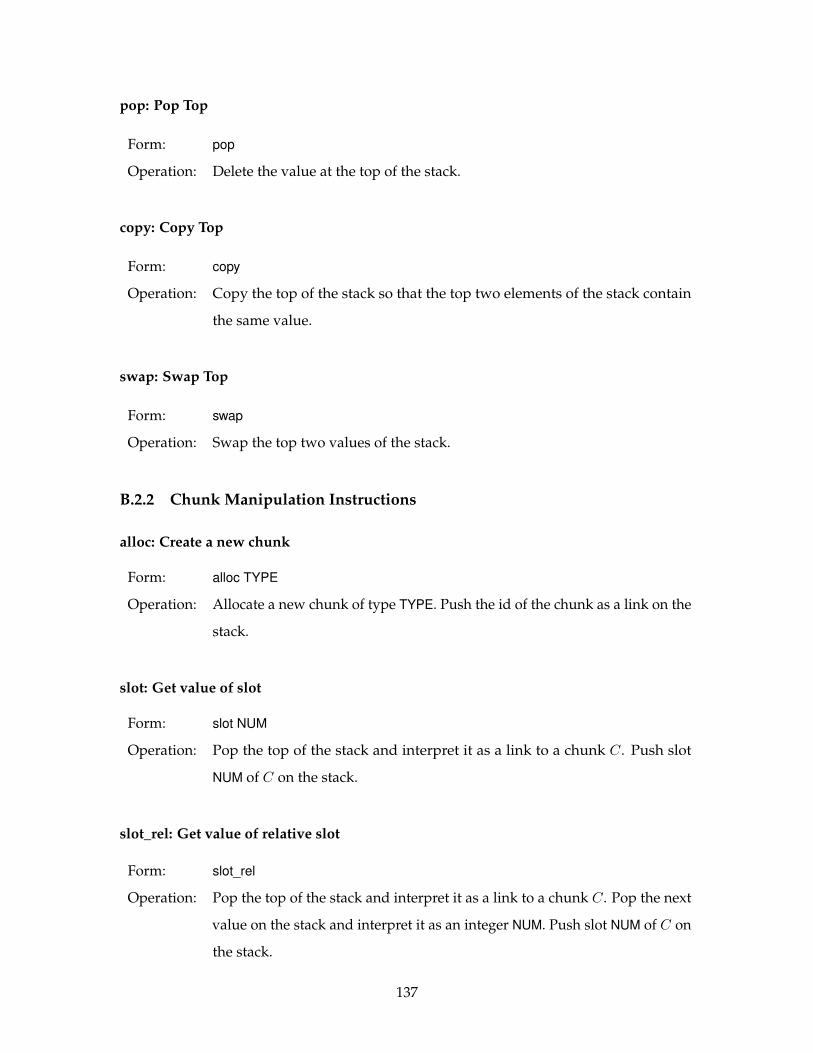
pop: Pop Top

Form: pop

Operation: Delete the value at the top of the stack.

copy: Copy Top

Form: copy

Operation: Copy the top of the stack so that the top two elements of the stack contain

the same value.

swap: Swap Top

Form: swap

Operation: Swap the top two values of the stack.

B.2.2 Chunk Manipulation Instructions

alloc: Create a new chunk

Form: alloc TYPE

Operation: Allocate a new chunk of type TYPE. Push the id of the chunk as a link on the

stack.

slot: Get value of slot

Form: slot NUM

Operation: Pop the top of the stack and interpret it as a link to a chunk C. Push slot

NUM of C on the stack.

slot_rel: Get value of relative slot

Form: slot_rel

Operation: Pop the top of the stack and interpret it as a link to a chunk C. Pop the next

value on the stack and interpret it as an integer NUM. Push slot NUM of C on

the stack.

137

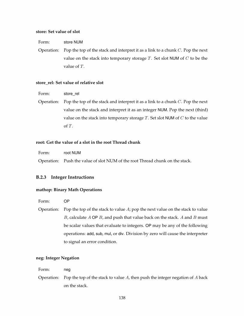
store: Set value of slot

Form: store NUM


value on the stack into temporary storage T . Set slot NUM of C to be the

value of T .

store_rel: Set value of relative slot

Form: store_rel


value on the stack and interpret it as an integer NUM. Pop the next (third)

value on the stack into temporary storage T . Set slot NUM of C to the value

of T .

root: Get the value of a slot in the root Thread chunk

Form: root NUM

Operation: Push the value of slot NUM of the root Thread chunk on the stack.

B.2.3 Integer Instructions

mathop: Binary Math Operations

Form: OP

Operation: Pop the top of the stack to value A; pop the next value on the stack to value

B, calculate A OP B, and push that value back on the stack. A and B must

be scalar values that evaluate to integers. OP may be any of the following

operations: add, sub, mul, or div. Division by zero will cause the interpreter

to signal an error condition.

neg: Integer Negation

Form: neg

Operation: Pop the top of the stack to value A, then push the integer negation of A back

on the stack.

138

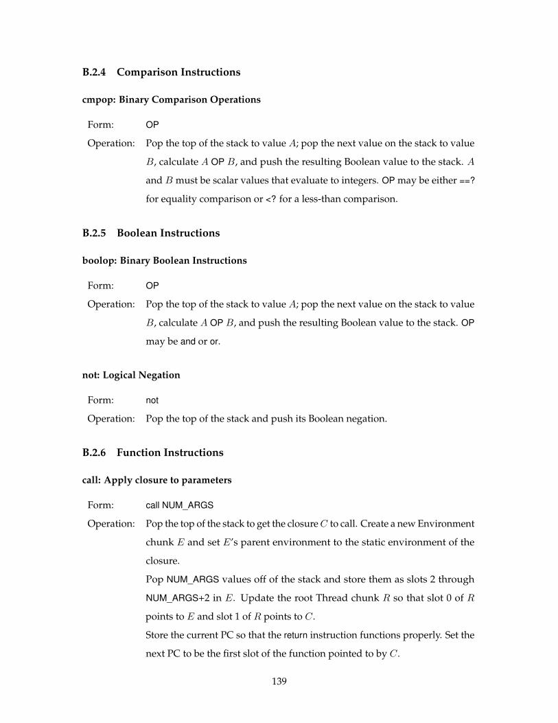
B.2.4 Comparison Instructions

cmpop: Binary Comparison Operations

Form: OP


B, calculate A OP B, and push the resulting Boolean value to the stack. A

and B must be scalar values that evaluate to integers. OP may be either ==?

for equality comparison or <? for a less-than comparison.

B.2.5 Boolean Instructions

boolop: Binary Boolean Instructions

Form: OP


B, calculate A OP B, and push the resulting Boolean value to the stack. OP

may be and or or.

not: Logical Negation

Form: not

Operation: Pop the top of the stack and push its Boolean negation.

B.2.6 Function Instructions

call: Apply closure to parameters

Form: call NUM_ARGS

Operation: Pop the top of the stack to get the closure C to call. Create a new Environment

chunk E and set E’s parent environment to the static environment of the

closure.

Pop NUM_ARGS values off of the stack and store them as slots 2 through

NUM_ARGS+2 in E. Update the root Thread chunk R so that slot 0 of R

points to E and slot 1 of R points to C.

Store the current PC so that the return instruction functions properly. Set the

next PC to be the first slot of the function pointed to by C.

139

return: Return from a procedure

Form: return NUM_RVALS

Operation: Pop the NUM_RVALS values off the top of the stack into temporary storage T ;

push the NUM_RVALS back on to the stack of the caller (if there is a different

stack). Restore the PC to the instruction after the one set by the most recent

call instruction.

system: Apply system function to arguments

Form: system NUM_ARGS

Operation: Pop the top of the stack to get the name of the system function to call. Pop

NUM_ARGS values off of the stack and use them as the arguments to the

function. Call the system function. When the function returns, push returned

values back on the stack.

B.3 Warts

There are two warts in the SCVM bytecode:

• Given the slot and store class of instructions, the root instruction should return the id

of the root chunk, rather than allowing only access to a slot. However, by hiding the

chunk ID of the Thread chunk, the SCVM interpreter can protect against writes to the

machine’s own slots in the root chunk.

• slot_rel and store_rel should be implemented slot and store with no argument passed.

140

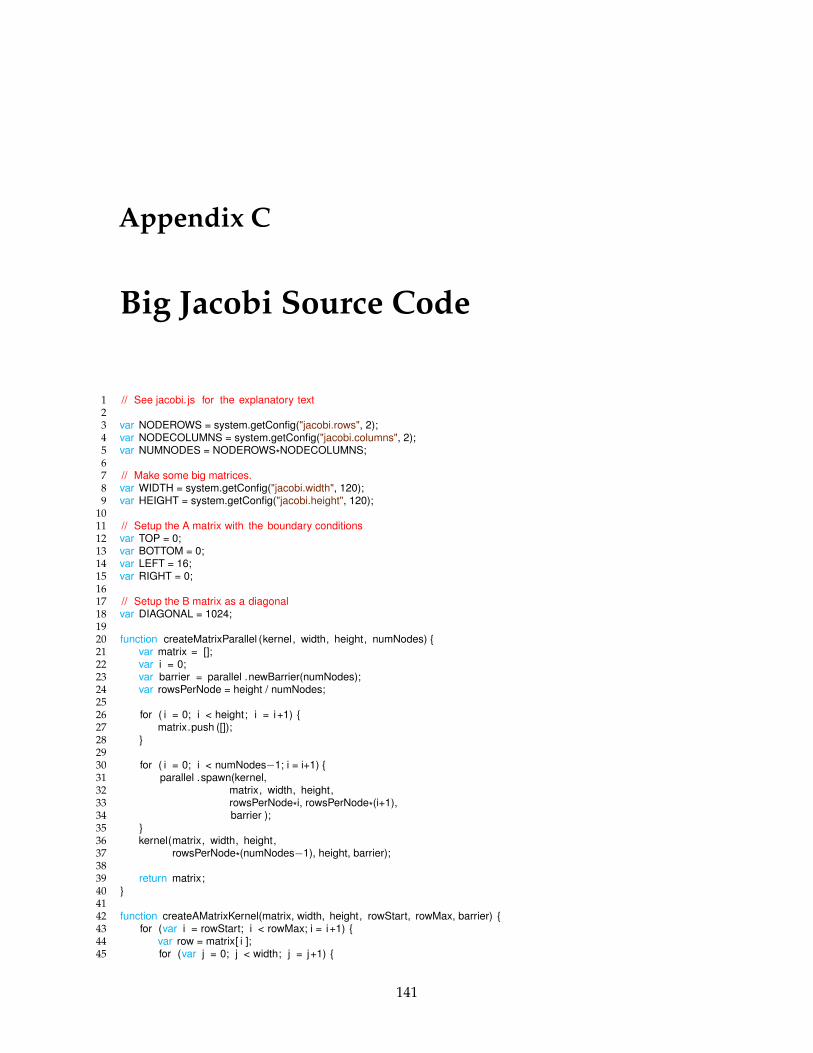
Appendix C

Big Jacobi Source Code

1 // See jacobi. js for the explanatory text23 var NODEROWS = system.getConfig("jacobi.rows", 2);4 var NODECOLUMNS = system.getConfig("jacobi.columns", 2);5 var NUMNODES = NODEROWS*NODECOLUMNS;67 // Make some big matrices.8 var WIDTH = system.getConfig("jacobi.width", 120);9 var HEIGHT = system.getConfig("jacobi.height", 120);

1011 // Setup the A matrix with the boundary conditions12 var TOP = 0;13 var BOTTOM = 0;14 var LEFT = 16;15 var RIGHT = 0;1617 // Setup the B matrix as a diagonal18 var DIAGONAL = 1024;1920 function createMatrixParallel (kernel, width, height, numNodes) {21 var matrix = [];22 var i = 0;23 var barrier = parallel .newBarrier(numNodes);24 var rowsPerNode = height / numNodes;2526 for ( i = 0; i < height; i = i+1) {27 matrix.push ([]);28 }2930 for ( i = 0; i < numNodes−1; i = i+1) {31 parallel .spawn(kernel,32 matrix, width, height,33 rowsPerNode*i, rowsPerNode*(i+1),34 barrier );35 }36 kernel(matrix, width, height,37 rowsPerNode*(numNodes−1), height, barrier);3839 return matrix;40 }4142 function createAMatrixKernel(matrix, width, height, rowStart, rowMax, barrier) {43 for (var i = rowStart; i < rowMax; i = i+1) {44 var row = matrix[ i ];45 for (var j = 0; j < width; j = j+1) {

141

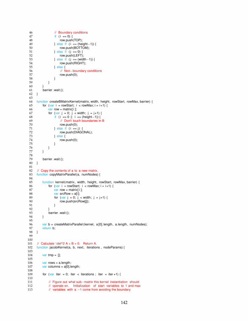
46 // Boundary conditions47 if ( i == 0) {48 row.push(TOP);49 } else if ( i == (height−1)) {50 row.push(BOTTOM);51 } else if ( j == 0) {52 row.push(LEFT);53 } else if ( j == (width−1)) {54 row.push(RIGHT);55 } else {56 // Non−boundary conditions57 row.push(0);58 }59 }60 }61 barrier .wait ();62 }6364 function createBMatrixKernel(matrix, width, height, rowStart, rowMax, barrier) {65 for (var i = rowStart; i < rowMax; i = i+1) {66 var row = matrix[ i ];67 for (var j = 0; j < width; j = j+1) {68 if ( i == 0 || i == (height−1)) {69 // Don't touch boundaries in B70 row.push(0);71 } else if ( i == j ) {72 row.push(DIAGONAL);73 } else {74 row.push(0);75 }76 }77 }7879 barrier .wait ();80 }8182 // Copy the contents of a to a new matrix.83 function copyMatrixParallel(a, numNodes) {8485 function kernel(matrix, width, height, rowStart, rowMax, barrier) {86 for (var i = rowStart; i < rowMax; i = i+1) {87 var row = matrix[ i ];88 var srcRow = a[i ];89 for (var j = 0; j < width; j = j+1) {90 row.push(srcRow[j]);91 }92 }93 barrier .wait ();94 }9596 var b = createMatrixParallel (kernel, a [0]. length, a.length, numNodes);97 return b;98 }99

100101 // Calculate \del^2 A + B = 0. Return A.102 function jacobiKernel(a, b, next, iterations , nodeParams) {103104 var tmp = [];105106 var rows = a.length;107 var columns = a[0].length;108109 for (var iter = 0; iter < iterations ; iter = iter +1) {110111 // Figure out what sub−matrix this kernel instantiation should112 // operate on. Initialization of start variables to 1 and max113 // variables with a −1 come from avoiding the boundary

142

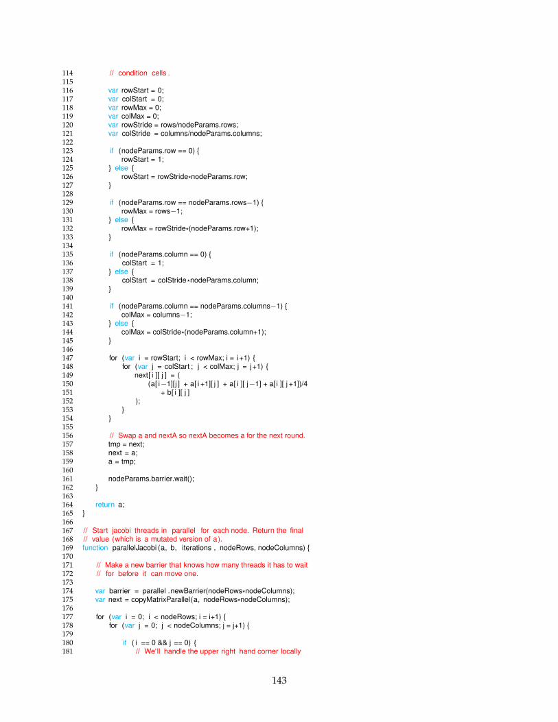
114 // condition cells .115116 var rowStart = 0;117 var colStart = 0;118 var rowMax = 0;119 var colMax = 0;120 var rowStride = rows/nodeParams.rows;121 var colStride = columns/nodeParams.columns;122123 if (nodeParams.row == 0) {124 rowStart = 1;125 } else {126 rowStart = rowStride*nodeParams.row;127 }128129 if (nodeParams.row == nodeParams.rows−1) {130 rowMax = rows−1;131 } else {132 rowMax = rowStride*(nodeParams.row+1);133 }134135 if (nodeParams.column == 0) {136 colStart = 1;137 } else {138 colStart = colStride*nodeParams.column;139 }140141 if (nodeParams.column == nodeParams.columns−1) {142 colMax = columns−1;143 } else {144 colMax = colStride*(nodeParams.column+1);145 }146147 for (var i = rowStart; i < rowMax; i = i+1) {148 for (var j = colStart ; j < colMax; j = j+1) {149 next[ i ][ j ] = (150 (a[ i−1][j ] + a[ i +1][ j ] + a[ i ][ j−1] + a[ i ][ j +1])/4151 + b[ i ][ j ]152 );153 }154 }155156 // Swap a and nextA so nextA becomes a for the next round.157 tmp = next;158 next = a;159 a = tmp;160161 nodeParams.barrier.wait();162 }163164 return a;165 }166167 // Start jacobi threads in parallel for each node. Return the final168 // value (which is a mutated version of a).169 function parallelJacobi (a, b, iterations , nodeRows, nodeColumns) {170171 // Make a new barrier that knows how many threads it has to wait172 // for before it can move one.173174 var barrier = parallel .newBarrier(nodeRows*nodeColumns);175 var next = copyMatrixParallel(a, nodeRows*nodeColumns);176177 for (var i = 0; i < nodeRows; i = i+1) {178 for (var j = 0; j < nodeColumns; j = j+1) {179180 if ( i == 0 && j == 0) {181 // We'll handle the upper right hand corner locally

143

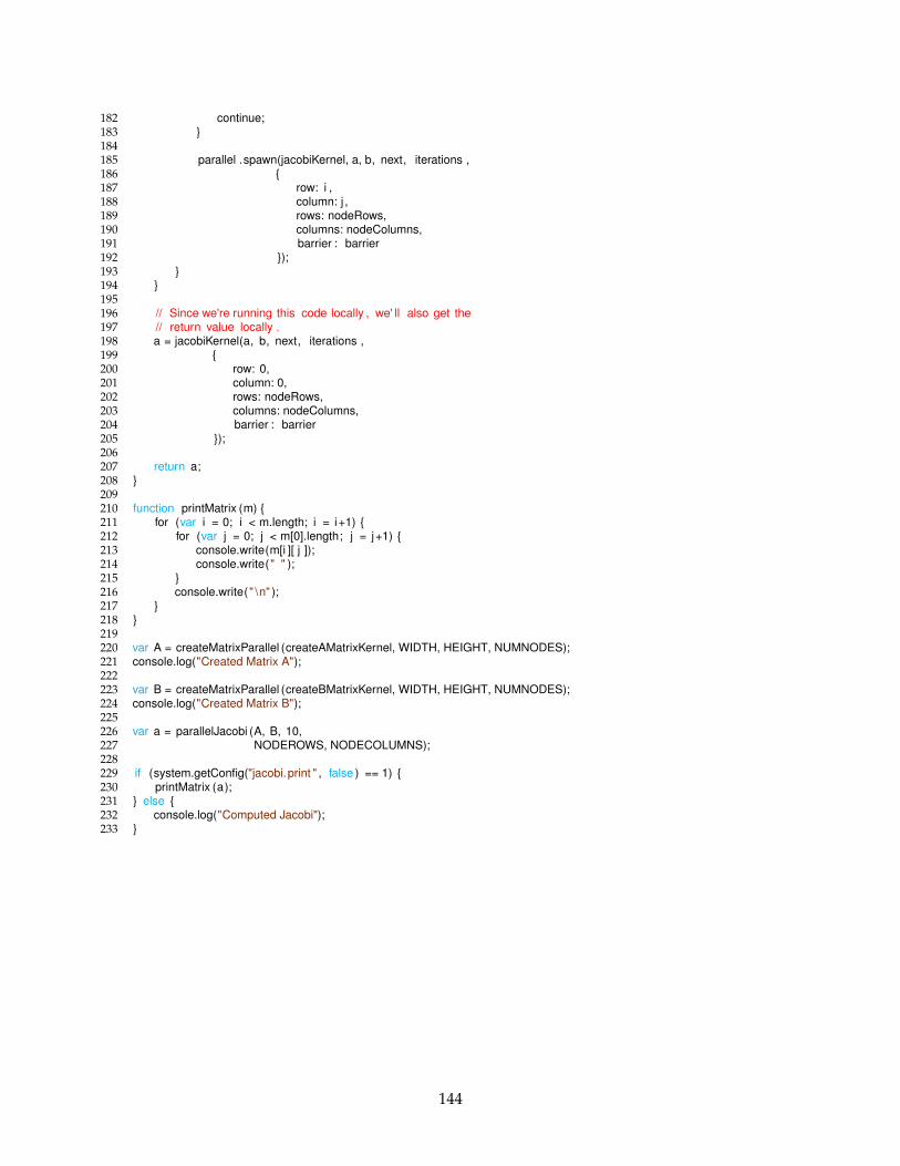
182 continue;183 }184185 parallel .spawn(jacobiKernel, a, b, next, iterations ,186 {187 row: i ,188 column: j ,189 rows: nodeRows,190 columns: nodeColumns,191 barrier : barrier192 });193 }194 }195196 // Since we're running this code locally , we' ll also get the197 // return value locally .198 a = jacobiKernel(a, b, next, iterations ,199 {200 row: 0,201 column: 0,202 rows: nodeRows,203 columns: nodeColumns,204 barrier : barrier205 });206207 return a;208 }209210 function printMatrix (m) {211 for (var i = 0; i < m.length; i = i+1) {212 for (var j = 0; j < m[0].length; j = j+1) {213 console.write(m[i ][ j ]);214 console.write(" " );215 }216 console.write(" \n" );217 }218 }219220 var A = createMatrixParallel (createAMatrixKernel, WIDTH, HEIGHT, NUMNODES);221 console.log("Created Matrix A");222223 var B = createMatrixParallel (createBMatrixKernel, WIDTH, HEIGHT, NUMNODES);224 console.log("Created Matrix B");225226 var a = parallelJacobi (A, B, 10,227 NODEROWS, NODECOLUMNS);228229 if (system.getConfig("jacobi.print " , false ) == 1) {230 printMatrix (a);231 } else {232 console.log("Computed Jacobi");233 }

144

Bibliography

[1] Information technology - generic coding of moving pictures and associated audioinformation: Video. Recommendation H.262, International Telecommunication Union,2000.

[2] Advanced video coding for generic audiovisual services. Recommendation H.264,International Telecommunication Union, May 2003.

[3] Material exchange format (MXF) — file format specification. Standard 377, SMPTE,2009.

[4] RTMP specification. Adobe developer connection, Adobe Systems Inc., January 2009.

[5] Saleh E. Abdullahi and Graem A. Ringwood. Garbage collecting the internet: A surveyof distributed garbage collection. ACM Computing Surveys, September 1998.

[6] Sarita V. Adve and Kourosh Gharachorloo. Shared memory consistency models: Atutorial. Computer, December 1996.

[7] Amazon. Amazon EC2 spot instances. http://aws.amazon.com/ec2/spot-instances/.

[8] Amazon. Amazon elastic compute cloud (EC2). http://aws.amazon.com/ec2/.

[9] Andrew Edward Ayers. M: A Memory Manager for L. M.S. thesis, MassachusettsInstitute of Technology, February 1988.

[10] David F. Bacon, Perry Cheng, and V. T. Rajan. A unified theory of garbage collection.ACM SIGPLAN Notices, 2004.

[11] Henry G. Baker Jr. List processing in real time on a serial computer. Communications ofthe ACM, 1978.

[12] Rajesh Krishna Balan, Mahadev Satyanarayanan, So Young Park, and Tadashi Okoshi.Tactics-based remote execution for mobile computing. In MobiSys, 2003.

[13] Andrew Baumann, Paul Barham, Pierre-Evariste Dagand, Tim Harris, Rebecca Isaacs,Simon Peter, Timothy Roscoe, Adrian Schüpbach, and Akhilesh Singhania. Themultikernel: A new OS architecture for scalable multicore systems. In SOSP, 2009.

[14] Nalini Belaramani, Jiandan Zheng, Amol Nayate, Robert Soulé, Mike Dahlin, andRobert Grimm. PADS: a policy architecture for distributed storage systems. In NSDI,2009.

145

[15] Peter Boehler Bishop. Computer Systems with a Very Large Address Space and GarbageCollection. Ph.D. thesis, Massachusetts Institute of Technology, May 1977.

[16] William J. Bolosky, Robert P. Fitzgerald, and Michael L. Scott. Simple but effectivetechniques for NUMA memory management. In SOSP, 1989.

[17] Silas Boyd-Wickizer, Haibo Chen, Rong Chen, Yandong Mao, Frans Kaashoek, RobertMorris, Alex Pesterev, Lex Stein, Ming Wu, Yuehua Dai, Yang Zhang, and ZhengZhang. Corey: An operating system for many cores. In OSDI, 2008.

[18] Gerard Briscoe and Alexandros Marinos. Digital ecosystems in the clouds: Towardscommunity cloud computing. In IEEE DEST, 2009.

[19] Vinny Cahill, Paddy Nixon, Brendan Tangney, and Fethi Rabhi. Object models fordistributed or persistent programming. The Computer Journal, August 1997.

[20] Brendon Cahoon and Kathryn S. McKinley. Data flow analysis for software prefetchinglinked data structures in java. In PACT, 2001.

[21] Brad Calder, Chandra Krintz, Simmi John, and Todd Austin. Cache-conscious dataplacement. In ASPLOS, 1998.

[22] Steve Carr, Kathryn S. McKinley, and Chau-Wen Tseng. Compiler optimizations forimproving data locality. In ASPLOS, 1994.

[23] Trishul M. Chilimbi, Bob Davidson, and James R. Larus. Cache-conscious structuredefinition. In PLDI, 1999.

[24] Trishul M. Chilimbi, Mark D. Hill, and James R. Larus. Cache-conscious structurelayout. In PLDI, 1999.

[25] Byung-Gon Chun, Sunghwan Ihm, Petros Maniatis, Mayur Naik, and Ashwin Patti.CloneCloud: elastic execution between mobile device and cloud. In EuroSys, 2011.

[26] Anthony Cozzie, Frank Stratton, Hui Xue, and Samuel T. King. Digging for datastructures. In OSDI, 2008.

[27] Eduardo Cuervo, Aruna Balasubramanian, Dae-ki Cho, Alec Wolman, Stefan Saroiu,Ranveer Chandra, and Paramvir Bahl. MAUI: making smartphones last longer withcode offload. In MobiSys, 2010.

[28] Eyal de Lara, Dan S. Wallach, and Willy Zwaenepoel. Puppeteer: Component-basedadaptation for mobile computing. In USITS, 2001.

[29] Jeffrey Dean and Sanjay Ghemawat. MapReduce: simplified data processing on largeclusters. In OSDI, 2004.

[30] Erik D. Demaine. Cache-oblivious algorithms and data structures. In Lecture Notesfrom the EEF Summer School on Massive Data Sets, 2002.

[31] Edsger W. Dijkstra, Leslie Lamport, A. J. Martin, C. S. Scholten, and E. F. M. Steffens.On-the-fly garbage collection: an exercise in cooperation. Communications of the ACM,November 1978.

146

[32] Dave Durkee. Why cloud computing will never be free. Communications of the ACM,May 2010.

[33] Robert R. Fenichel and Jerome C. Yochelson. A LISP garbage-collector for virtual-memory computer systems. Communications of the ACM, November 1969.

[34] Ian Fette and Alexey Melnikov. The WebSocket protocol. RFC 6455, IETF, December2011.

[35] Joseph A. Fisher, John R. Ellis, John C. Ruttenberg, and Alexandru Nicolau. Parallelprocessing: A smart compiler and a dumb machine. ACM SIGPLAN Notices, 1984.

[36] Jason Flinn, Dushyanth Narayanan, and Mahadev Satyanarayanan. Self-tuned remoteexecution for pervasive computing. In HotOS, May 2001.

[37] Matteo Frigo, Charles E. Leiserson, Harald Prokop, and Sridhar Ramachandran. Cache-oblivious algorithms. In Foundations of Computer Science, 1999.

[38] Alfonso Fuggetta, Gian Pietro Picco, and Giovanni Vigna. Understanding code mobility.IEEE Transactions on Software Engineering, May 1998.

[39] Ben Gamsa, Orran Krieger, and Jonathan Appavoo. Tornado: Maximizing locality andconcurrency in a shared memory multiprocessor operating system. In OSDI, 1999.

[40] Nikolas Gloy, Trevor Blackwell, Michael D. Smith, and Brad Calder. Procedure place-ment using temporal ordering information. In MICRO, 1997.

[41] Íñigo Goiri, Jordi Guitart, and Jordi Torres. Characterizing cloud federation for en-hancing providers’ profit. In IEEE CLOUD, 2010.

[42] Google. Google app engine. https://developers.google.com/appengine/.

[43] Google. The task queue python API. https://developers.google.com/appengine/docs/python/taskqueue/.

[44] Kinshuk Govil, Dan Teodosiu, Yongqiang Huang, and Mendel Rosenblum. Cellulardisco: Resource management using virtual clusters on shared-memory multiprocessors.ACM Transactions on Computer Systems, August 2000.

[45] Elana D Granston and Harry A. G Wijshoff. Managing pages in shared virtual memorysystems: getting the compiler into the game. In ICS, 1993.

[46] Lei Guo, Songqing Chen, Zhen Xiao, and Xiaodong Zhang. Analysis of multimediaworkloads with implications for internet streaming. In WWW, 2005.

[47] Robert Hunter Halstead Jr. Reference Tree Networks : Virtual Machine and Implementation.Ph.D. thesis, Massachusetts Institute of Technology, July 1979.

[48] Robert Hunter Halstead Jr. and Stephen A. Ward. The MuNet: a scalable decentralizedarchitecture for parallel computation. In ISCA, 1980.

[49] Harold Abelson, Gerald Jay Sussman, and Julie Sussman. Structure and Interpretation ofComputer Programs. The MIT Press, Cambridge, Massachusetts, second edition, 1996.

147

[50] Mark D. Hill. Multiprocessors should support simple memory consistency models.Computer, August 1998.

[51] Michael Hind. Pointer analysis: Haven’t we solved this problem yet? In PASTE, 2001.

[52] Benjamin Hindman, Andy Konwinski, Matei Zaharia, Ali Ghodsi, Anthony D. Joseph,Randy Katz, Scott Shenker, and Ion Stoica. Mesos: A platform for fine-grained resourcesharing in the data center. In NSDI, 2011.

[53] Martin Hirzel, Amer Diwan, and Matthew Hertz. Connectivity-based garbage collec-tion. In OOPSLA, volume 38, 2003.

[54] Martin Hirzel, Johannes Henkel, Amer Diwan, and Michael Hind. Understanding theconnectivity of heap objects. In ISMM, 2002.

[55] Richard L. Hudson and J. Eliot B. Moss. Incremental collection of mature objects. InIWMM, 1992.

[56] Daniel Hughes, Geoff Coulson, and James Walkerdine. Free riding on gnutella revis-ited: The bell tolls? IEEE Distributed Systems Online, June 2005.

[57] Michael Isard, Mihai Budiu, Yuan Yu, Andrew Birrell, and Dennis Fetterly. Dryad:Distributed data-parallel programs from sequential building blocks. In EuroSys, 2007.

[58] Sokol Kosta, Andrius Aucinas, Pan Hui, Richard Mortier, and Xinwen Zhang. ThinkAir:dynamic resource allocation and parallel execution in the cloud for mobile code of-floading. In IEEE INFOCOM, March 2012.

[59] Bassam Kurdali. Elephants dream. http://orange.blender.org/, 2006.

[60] Kristian Kvilekval and Ambuj K. Singh. SPREE: object prefetching for mobile comput-ers. In DOA, volume 3291, 2004.

[61] Leslie Lamport. How to make a multiprocessor computer that correctly executesmultiprocess programs. IEEE Transactions on Computers, September 1979.

[62] Ang Li, Xiaowei Yang, Srikanth Kandula, and Ming Zhang. CloudCmp: comparingpublic cloud providers. In IMC, 2010.

[63] Henry Lieberman and Carl Hewitt. A real-time garbage collector based on the lifetimesof objects. Communications of the ACM, June 1983.

[64] Erik Lindholm, John Nickolls, Stuart Oberman, and John Montrym. NVIDIA tesla: Aunified graphics and computing architecture. IEEE Micro, April 2008.

[65] Chi-Keung Luk. Tolerating memory latency through software-controlled pre-executionin simultaneous multithreading processors. In ISCA, 2001.

[66] Ming Mao, Jie Li, and Marty Humphrey. Cloud auto-scaling with deadline and budgetconstraints. In GRID, 2010.

[67] Matroska. Matroska specifications. http://www.matroska.org/technical/specs/index.html.

[68] John McCarthy. Recursive functions of symbolic expressions and their computationby machine, part i. Communications of the ACM, April 1960.

148

[69] Microsoft. AVI RIFF file reference. http://msdn.microsoft.com/en-us/library/ms779636.aspx.

[70] Microsoft. Windows azure: Microsoft’s cloud platform. http://www.windowsazure.com/en-us/.

[71] Joseph Derek Morrison. A Scalable Multiprocessor Architecture using Cartesian Network-Relative Addressing. M.S. thesis, Massachusetts Institute of Technology, September1989.

[72] Andreas Moshovos, Dionisios N. Pnevmatikatos, and Amirali Baniasadi. Slice-processors: An implementation of operation-based prediction. In ICS, 2001.

[73] J. Eliot B. Moss. Design of the mneme persistent object store. ACM Transactions onInformation Systems, April 1990.

[74] Brian D. Noble, Mahadev Satyanarayanan, Dushyanth Narayanan, James Eric Tilton,Jason Flinn, and Kevin R. Walker. Agile application-aware adaptation for mobility. InSOSP, 1997.

[75] Object Management Group. The common object request broker: Architecture andspecification. http://www.omg.org/spec/CORBA/.

[76] Mark Palmer and Stanley Zdonik. Fido: A cache that learns to fetch. In VLDB, 1991.

[77] Justin Mazzola Paluska and Hubert Pham. Interactive streaming of structured data. InPerCom, 2010.

[78] Justin Mazzola Paluska, Hubert Pham, Gregor Schiele, Christian Becker, and SteveWard. Vision: a lightweight computing model for fine-grained cloud computing. InACM MCS, 2012.

[79] Justin Mazzola Paluska, Hubert Pham, and Steve Ward. ChunkStream: interactivestreaming of structured data. Pervasive and Mobile Computing, 2010.

[80] Justin Mazzola Paluska, Hubert Pham, and Steve Ward. Structuring the unstructuredmiddle with chunk computing. In HotOS, 2011.

[81] Roger Pantos and William May Jr. HTTP live streaming. Internet Draft draft-pantos-http-live-streaming-11, IETF, April 2013.

[82] Mark S. Papamarcos and Janak H. Patel. A low-overhead coherence solution formultiprocessors with private cache memories. In ISCA, 1984.

[83] R. Hugo Patterson, Garth A. Gibson, and Mahadev Satyanarayanan. A status report onresearch in transparent informed prefetching. ACM SIGOPS Operating Systems Review,April 1993.

[84] Mahadev Satyanarayanan, Paramvir Bahl, Ramón Cáceres, and Nigel Davies. The casefor VM-Based cloudlets in mobile computing. IEEE Pervasive Computing, October 2009.

[85] Henning Schulzrinne, Stephen L. Casner, Ron Frederick, and Van Jacobson. RTP: atransport protocol for real-time applications. RFC 1889, IETF, January 1996.

149

[86] Henning Schulzrinne, Anup Rao, and Robert Lanphier. Real time streaming protocol(RTSP). RFC 2326, IETF, April 1998.

[87] Marc Shapiro, Peter Dickman, and David Plainfossé. SSP chains: Robust, distributedreferences supporting acyclic garbage collection. Rapport de Recherche 1799, INRIA,November 1992.

[88] Sun Microsystems. Jini component system. http://www.jini.org.

[89] Chunqiang Tang, DeQing Chen, Sandhya Dwarkadas, and Michael L. Scott. Integratingremote invocation and distributed shared state. In IPDPS, 2004.

[90] David Wentzlaff and Anant Agarwal. Factored operating systems (fos): The case fora scalable operating system for multicores. SIGOPS Operating Systems Review, April2009.

[91] David Wentzlaff, Peter Griffin, Henry Hoffmann, Liewei Bao, Bruce Edwards, CarlRamey, Matthew Mattina, Chyi-Chang Miao, John F. Brown III, and Anant Agarwal.On-chip interconnection architecture of the tile processor. IEEE Micro, September 2007.

[92] Adam Wolbach, Jan Harkes, Srinivas Chellappa, and Mahadev Satyanarayanan. Tran-sient customization of mobile computing infrastructure. In MobiVirt, 2008.

[93] Michael E. Wolf and Monica S. Lam. A data locality optimizing algorithm. In PLDI,1991.

[94] Seungjun Yang, Yongin Kwon, Yeongpil Cho, Hayoon Yi, Donghyun Kwon, JongheeYoun, and Yunheung Paek. Fast dynamic execution offloading for efficient mobilecloud computing. In PerCom, 2013.

[95] Michael Young, Avadia Tevanian, Richard Rashid, David Golub, Jeffrey Eppinger,Jonathan Chew, William Bolosky, David Black, and Robert Baron. The duality ofmemory and communication in the implementation of a multiprocessor operatingsystem. In SOSP, 1987.

[96] Yuan Yu, Michael Isard, Dennis Fetterly, Mihai Budiu, Úlfar Erlingsson, Kumar Gunda,and Jon Currey. DryadLINQ: a system for general-purpose distributed data-parallelcomputing using a high-level language. In OSDI, 2008.

150

Computing with Chunks - MIT...

Documents

Transcript of Computing with Chunks - MIT...