Computing the Uncomputable,

or,

The Discrete Charm of Second-Order Simulacra

Matthew W. Parker Department of Philosophy, Logic and Scientific Method

London School of Economics

Updated July 2008

Abstract. We examine a case in which non-computable behavior in a

model is revealed by computer simulation. This is possible due to differing notions of computability for sets in a continuous space. The argument originally given for the validity of the simulation involves a simpler simulation of the simulation, still further simulations thereof, and a universality conjecture. There are difficulties with that argument, but there are other, heuristic arguments supporting the qualitative results. It is urged, using this example, that absolute validation, while highly desirable, is overvalued. Simulations also provide valuable insights that we cannot yet (if ever) prove.

If we could take as the finest allegory of simulation the Borges tale where the cartographers of the Empire draw up a map so detailed that it ends up exactly covering the territory…, this fable would then have come full circle for us, and now has nothing but the discrete charm of second-order simulacra.

—Jean Baudrillard, Simulacra and Simulation

1. Introduction

The absurd map of Borges and Casares ([1946] 1999) to which Baudrillard

alludes should be well known among those who study modeling and simulation. The

2

short parable that describes it is even titled “Of Rigor in Science” (“Del Rigor en la

Ciencia”). Rigor, it thus suggests, can be excessive. Lewis Carroll describes a similar

map, which is never unfurled due to socioeconomic obstacles ([1893] 2005). "[W]e now

use the country itself, as its own map,” a character explains, “and I assure you it does

nearly as well.” The joke, of course, is that the map would have done nearly as badly. A

useful representation is not a perfect replica; it must be somehow more manageable than

its object.

One valuable kind of manageability today is realizability on a digital computer.

This is not always feasible; a system may be too complex to usefully simulate “in silico.”

If a computer simulation is attempted, we would like to validate it, that is, to show that

the simulation results must hold as well for the process simulated. But this too might

prove impossible, or merely unattainable in practice.

Here we examine a case of simulation (Sommerer and Ott 1996) that is

remarkable in several respects. Firstly, it seems to show that the long-term behavior of a

certain simple, deterministic physical system is strictly non-computable; no program can

reliably decide whether the state of the system will tend toward one set of states or

another. This is interesting in itself, especially since in this case not only is quantitative

prediction undermined by inevitable measurement error, but even the qualitative

behavior of the system (in particular, which attractor1 it approaches) is unpredictable for

1 Here, ‘attractor’ is used in a sense similar to that of Milnor (1985): essentially, it is a

set whose basin of attraction has positive measure. The basin of attraction of a set A is the union of all orbits that asymptotically approach A. Under other definitions of attractor, all points near an attractor must lie in its basin, so the complex “riddled” basins discussed here are ruled out.

3

computational reasons. But secondly, how is this non-computability established? Why,

by computer simulation of course—computing the uncomputable! We will see how this

is possible. Thirdly, the scientists argue for the validity of their simulations—of a

continuous-time dynamical system—by reference to a simpler, and discrete-time,

simulation of the simulation (hence my alternate title). In fact, this second simulation is

in turn studied by means of third- and fourth-order simulations.2 This illustrates the

already appreciated variety of hats that models and simulations wear: among other

things, they can act in chains to supply analysis and support of one another. (Cf. Gelfert

2006.)

Those are just preliminary remarks. My main claims are four:

(i) Sommerer and Ott’s validation argument ultimately fails. It appeals to an

absolute “universality” conjecture: that all systems of a particular kind exhibit a certain

“power-law scaling” phenomenon. However, this is not true in any sense that would

support their argument, and the appeal to it appears to be circular. Morton claims that

“the core of any systematic modeling along these lines [charting the attractors of

simplified models] has to be some very general mathematical treatment of

‘universality’...” (1993, 666). But no rigorous treatment of universality succeeds here.

(ii) Nonetheless, the second-order simulations provide strong evidence, by means

2 These last three simulations are not run on a computer; they are abstract processes

studied analytically. Nonetheless they are processes, in which a model imitates the time evolution of another system. Hence they fit Hartmann’s definition of simulation (1996), except that they perhaps do not imitate “real” systems. They also have another important feature of scientific simulations: their behavior is not stipulated directly, but unfolds from a model or procedure. We discover their behavior, rather than imposing it.

4

of analogy, insight into mechanisms, and structural stability: the insensitivity of certain

properties to small modifications of the system.

(iii) Strict validation, i.e., proof that the results of a simulation hold for the target

system, is of course desirable, but should not always be demanded. Chaitin (1993)

argues that one of the great values of computer experiments is that they yield insights that

we cannot prove without adopting new axioms. Even if this is not strictly true,

simulations can at least indicate facts that we have not yet been able to prove, and

perhaps never will. Strict validation would render a simulation essentially deductive, so

if we insist on it, we deprive ourselves of a valuable complement to deduction.

(iv) Models and simulations need not represent any particular real system to be

valuable. This is hardly a new insight; highly non-physical models have long been used

in the study of nonlinear dynamics, for example.3 Yet most simulations discussed in the

philosophical literature represent specific actual processes (e.g., Morton 1993; Hartmann

1996; Winsberg 2001, 2003), and Hartmann’s definition of simulation requires an

instantiated target system. Sommerer and Ott’s simulations only imitate an abstract

model that itself takes Morgan and Morrison’s (1999) “autonomy” to extremes: it

appeals to no specific dynamical theory describing particular processes or forces, nor to

any particular systems in the actual world. It represents a purely hypothetical system that

only makes incidental use of very general concepts from mechanics (potential, force,

friction). Certainly it is intended to deliver some physical insight, but not into any

antecedently targeted system. Rather it illustrates general possibilities, and in so doing,

3 Thanks to a referee for this point.

5

reveals what strange behavior and epistemological recalcitrance can be expected from

many different physical systems. This further supports point (iii). While “questions of

trustworthiness” (Morton 1993) are critical when predicting the specific states of actual

systems, not so for more general purposes. Simulations can teach and explain without

any certification, by suggesting inductive hypotheses and informing our expectations—by

revealing general features of how things could go.

These last two claims will be illustrated by Sommerer and Ott’s investigations,

and then argued more explicitly in Section 7.

2. Sommerer and Ott’s continuous system

Sommerer and Ott (1996) describe their system as a point particle moving in a

two-dimensional potential, periodically “kicked” by an additional force. The motion is

governed by a second-order differential equation (which we omit) in two real variables, x

and y. The equation has terms representing (1) friction, (2) a certain potential V defined

by a polynomial in x and y (Figure 1(a)), and (3) a periodically oscillating force in the x-

direction. The space of possible states for this system has five dimensions: x, y, their

time derivatives, and since the periodic force is time-dependent, time itself.

Sommerer and Ott’s equation is not designed to represent any particular, actual

physical system. While the authors speak of a particle in a potential, it is plain that their

study is meant to be more general. In Ott and Sommerer 1994 they suggest that riddled

basins might occur in some chemical reaction-diffusion systems, and Heagey et al. (1994)

had already observed similar behavior in an electric circuit. The equation is built on the

6

two-well Duffing equation, which has been used to model the vibration of beams, but no

such practical purpose is know for the 1996 variant. Rather, the potential V seems to

have been contrived specifically to exemplify a certain strange kind of behaviour.

To gain a sense of the mechanisms governing Sommerer and Ott’s system,

imagine a marble rolling around on the curved surface V (Figure 1). Now, to represent

the periodic force, picture this surface rocking steadily to the left and right. Due to

friction, the marble will tend to settle into one of the two dips in the potential, but due to

the periodic force it will continue to roll left and right (very erratically in fact) within that

dip, approximately along the x-axis. While friction drags it toward the x-axis, the bump

between the dips contributes an element of instability: if our marble rolls up onto the

bump, it will tend to fall away from the x-axis. This can occur no matter how closely the

marble has settled in near the x-axis, as long as it does not roll exactly along that axis

from the outset.

Importantly, the subspace y = dy/dt = 0 of the state space, where our marble does

roll exactly along the x-axis, is an invariant manifold: orbits within it stay in it. This is

because Sommerer and Ott’s differential equation is symmetric in y. Orbits on this

invariant manifold form a closed subsystem governed by the two-well Duffing equation,

with three important properties: (1) It has two attractors within the invariant manifold,

(2) motion on these attractors appears to be chaotic,4 and (3) embedded in the larger

4 The important sort of “chaos” here is mere ergodicity, for we wish to use a theorem that

requires just that. Some regard ergodicity as insufficient for true chaos (see Berkovitz et al. 2006; thanks to a referee for this). Sommerer and Ott (1996) provide no evidence that the Duffing system is ergodic, and I do not know whether it has been proven elsewhere. Ku and Sun (1990)

7

Figure 1. Sommerer and Ott’s potential. Behavior of the system resembles that of a marble rolling on this surface as the latter rocks left and right. Graph (a) shows the potential V unaltered (except for the flattening at the top of the graph, which is an artifact of the graphing software). Graphs (b) and (c) show close-ups of the potential with rocking.

provide a range of computer generated images suggesting sensitive dependence on initial conditions and intuitive irregularity, as well as further references.

-1.245

0

1.2450.498

0

-0.498x

y

-1.245

0

1.2450.498

0

-0.498x

y

-2.475

0

2.4750.99

0

-0.99x

y

V(x, y)

(a)

(b) (c)

8

Figure 2. Orbits of Sommerer and Ott’s system. Position coordinates (x and y) of two different orbits (one black, one grey) with very nearby initial conditions are shown. The length of the bar at the bottom of each graph indicates time elapsed since the initial states. (a) The two orbits are so similar that the grey orbit conceals the black completely. (b) The orbits soon diverge. (c) Both orbits soon settle down very close to the x-axis, as shown by the straight black line there. (d) After a long time, one orbit becomes erratic and escapes to the other attractor, where it will probably stay. Thus two nearly indistinguishable initial states result in orbits approaching different attractors. system, these attractors have negative transverse Lyapunov exponents5; that is, if an orbit

on one of these attractors for the submanifold is perturbed off the submanifold, it will

tend to a return. It follows from these properties, by a theorem of Alexander et al.

(1991), that the two attractors for the subsystem are also attractors for the larger original

5 Lyapunov exponents are numbers that characterize the average exponential rate at

which orbits close to a given orbit diverge from the latter (if an exponent is positive) or converge toward it (if negative). Sommerer and Ott show analytically that the exponents for motion orthogonal to the invariant manifold are negative.

(a)

(c)

(b)

(d)

9

system, so that many orbits within the full five-dimensional state space are drawn to the

attractors within the invariant manifold. Hence in many cases our marble will get stuck

in one dip forever.

3. Computing the uncomputable

Sommerer and Ott run simulations like those shown in Figure 2 for every initial

state in a large two-dimensional grid, representing a slice through the state space. Each

initial state in the grid is associated with a pixel in a graph, which is colored black if the

associated orbit eventually gets very close to one attractor, and white if it gets very close

to the other. Thus the authors generate graphs of the two basins (shown in 1996 and

Parker 2003 and 2005), which suggest that the basins are intermingled: every tiny

neighborhood contains positive-measure portions of both basins. Since the basins are

disjoint, they are also riddled: in any neighborhood, the complement of a basin has

positive measure.

The non-computability argument then proceeds as follows: due to intermingling,

any procedure to determine in which basin a state lies would have to make full use of the

exact initial conditions. But this cannot be done by a Turing machine, for it would

require reading an infinite string of digits in finite time. Ergo, the basins are non-

computable.

However, it turns out that nearly all sets of real n-tuples—all except the null set

and Rn—are undecidable in a strict and very natural sense. (See, e.g., Weihrauch 2000.)

Without special clarification, undecidability claims in the continuous context are trivial.

10

But Sommerer and Ott’s argument is not; what it really shows is that if the basins are

intermingled, then they are not decidable up to measure zero, or d.m.z. (Parker 2005,

2006; called µ-decidability in Parker 2003). A set is d.m.z. if some decision procedure

gives the correct output for all possible inputs x ∈ Rn except possibly those inputs in

some set with zero volume. In particular, no riddled set with positive measure is d.m.z.

(Parker 2003, 2005). Every decision procedure for such a riddled, positive-measure set

will fail in a significant portion of cases. If the volume of a set of states reflects the

probability that a state in that set will occur, then any decision procedure for a non-d.m.z.

set will have a significant chance of failing.

Interestingly, Sommerer and Ott’s non-computability argument is itself founded

on computer simulations. They address this puzzling fact informally, in effect arguing

that their basins are recursively approximable,6 or r.a. (Ko 1991): there is a decision

procedure that will succeed with as small a non-zero error rate as you like. (If supplied a

whole-number parameter n, the decision procedure must give the correct output for any

input point except perhaps those in some set with measure less than 2-n. And unlike

d.m.z., r.a. requires that the procedure always halts.) If this holds, it is possible to

generate a graph of the basins that is arbitrarily accurate with respect to measure (Parker

2005), revealing measure-theoretic properties such as riddling.

Sommerer and Ott do not use the term ‘r.a.’ or define such a concept, but their

argument suggests it. They wish to validate their graphs, which are generated by

6 Sommerer and Ott do not use this term or define such a concept, but their argument

suggests it.

11

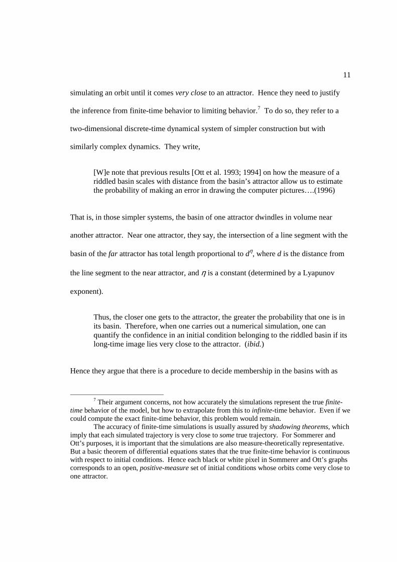
simulating an orbit until it comes very close to an attractor. Hence they need to justify

the inference from finite-time behavior to limiting behavior.7 To do so, they refer to a

two-dimensional discrete-time dynamical system of simpler construction but with

similarly complex dynamics. They write,

[W]e note that previous results [Ott et al. 1993; 1994] on how the measure of a riddled basin scales with distance from the basin’s attractor allow us to estimate the probability of making an error in drawing the computer pictures….(1996)

That is, in those simpler systems, the basin of one attractor dwindles in volume near

another attractor. Near one attractor, they say, the intersection of a line segment with the

basin of the far attractor has total length proportional to dη, where d is the distance from

the line segment to the near attractor, and η is a constant (determined by a Lyapunov

exponent).

Thus, the closer one gets to the attractor, the greater the probability that one is in its basin. Therefore, when one carries out a numerical simulation, one can quantify the confidence in an initial condition belonging to the riddled basin if its long-time image lies very close to the attractor. (ibid.)

Hence they argue that there is a procedure to decide membership in the basins with as

7 Their argument concerns, not how accurately the simulations represent the true finite-

time behavior of the model, but how to extrapolate from this to infinite-time behavior. Even if we could compute the exact finite-time behavior, this problem would remain.

The accuracy of finite-time simulations is usually assured by shadowing theorems, which imply that each simulated trajectory is very close to some true trajectory. For Sommerer and Ott’s purposes, it is important that the simulations are also measure-theoretically representative. But a basic theorem of differential equations states that the true finite-time behavior is continuous with respect to initial conditions. Hence each black or white pixel in Sommerer and Ott’s graphs corresponds to an open, positive-measure set of initial conditions whose orbits come very close to one attractor.

12

much statistical accuracy as one likes, short of 100 percent. This is the central feature of

recursive approximability.

This argument makes it plausible that the graphs are accurate, but it is far from a

proof. It mentions no reason to expect similar scaling behavior in the continuous system

except that both systems seem to have riddled basins. But this is circular; the evidence

that the continuous system exhibits riddling at all is precisely what they are trying to

validate. One might try to save the argument by further specifying the universality class.

If the scaling (and existence) of riddled basins were uniform for some class of systems

clearly including both the 1994 and 1996 systems, this might suffice. Sadly, no such law

holds, at least not of the kind that Sommerer and Ott need. As we will see, riddled basins

can scale as fast or slow as you like.

4. The 1994 discrete system

We now examine a slight generalization of one of the discrete systems from Ott et

al. 1994, the one most similar to the 1996 continuous system. Our version consists of

iterations of a non-invertible map ϕ on the rectangle X = [0, 1] × [-1, 1] with the

following general properties:

(i) It takes y-values toward 1 or –1, depending on x.

(ii) Its effect on x-coordinates is a stretch-and-fold operation similar to the Bernoulli shift φ(x) = 2x mod 1.

Due to (ii), motion in the x-direction is random in a sense to be explained. Since motion

13

in the y-direction depends on the x-coordinate, it will be random too, but in a different

sense. Despite this random motion, the top and bottom edges of the rectangle—let us call

them A+ and A− —turn out to be attractors.

To be more concrete, choose a curve x = α(y) that divides the rectangle into left

and right sections, with α(1) < ½ < α(−1). (See Figure 3(a).) For now, assume with

Sommerer and Ott that near the edges A+ and A−, this curve is straight and vertical. Next,

choose a bijection f: [–1, 1] → [–1, 1] such that f i(y) → 1 and f −i(y) → −1 as i → ∞.8

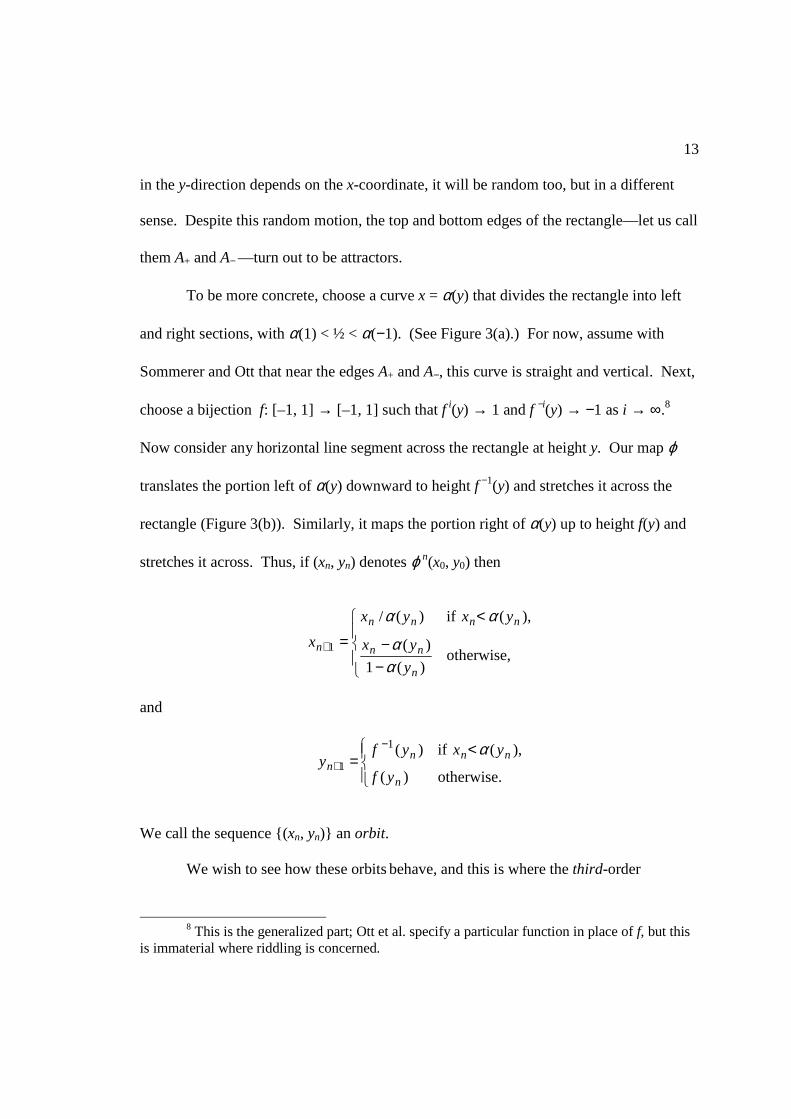
Now consider any horizontal line segment across the rectangle at height y. Our map ϕ

translates the portion left of α(y) downward to height f −1(y) and stretches it across the

rectangle (Figure 3(b)). Similarly, it maps the portion right of α(y) up to height f(y) and

stretches it across. Thus, if (xn, yn) denotes ϕ n(x0, y0) then

−−

<

=+otherwise,

)(1

)(

),( if)(/

1

n

nn

nnnn

n

y

yx

yxyx

x

αα

αα

and

<

=−

+otherwise.)(

),( if)(1

1n

nnnn

yf

yxyfy

α

We call the sequence {(xn, yn)} an orbit.

We wish to see how these orbits behave, and this is where the third-order

8 This is the generalized part; Ott et al. specify a particular function in place of f, but this

is immaterial where riddling is concerned.

14

Figure 3. A discrete-time dynamical system with intermingled basins. Based on Ott et al. 1994. Part (a) shows the domain of the map ϕ with schematics of the functions α and f from which ϕ is constructed. Part (b) shows the operation of ϕ on a horizontal line segment: the left portion is stretched and lowered while the right is stretched and raised.

simulacrum enters: following Sommerer and Ott, we model ϕ as a (spatially

inhomogeneous9) random walk. (The fourth-order simulacrum is the diffusion

approximation that Sommerer and Ott use to study the random walk; we will not discuss

it here.) For given initial conditions (x0, y0), each (xn, yn) will fall on some horizontal at y

= f i(y0) with i an integer. Such horizontals form a ladder with infinitely many rungs

between A− and A+. Define a probability measure on each of these horizontal rungs

identical to Lebesgue measure, so that the probability associated with a subset of a

9 This means that the probability of a step in a given direction varies from one position to

the next.

(a) (b)

A+

A−

15

horizontal is just the total length of that subset. On this probability measure, it turns out

that motion in the x-direction is random in the sense that the “probable” value of xn is

independent of its history {xi} i < n with regard to whether or not xi < α(yi) for each i

(Parker 2005). Hence the truth values of the propositions ‘x0 < α(y0)’, ‘ x1 < α(y1)’, ‘ x2 <

α(y2)’, etc., are as random as coin tosses (with the coin biased by the value α(yi) at each

toss). The same “coin tosses”, then, determine whether the y-coordinate will step up or

down at a given time, so the sequence of y-values forms a random walk over the values f

i(y0). (If we then map these values onto the integers, we have a spatially inhomogeneous

random walk over the integers.)

Using known results about random walks, and the provisional assumption that α

is constant near A+ and A− , Ott et al. show that A+ and A− are attractors, and near them,

their basins scale in a very regular way. The measure of the basin of A− on any horizontal

y = f i(0) close to A+ turns out to be B[α+/(1 − α+)]i , for some constant B (1994)10. For Ott

et al.’s particular choice of f, this equals +− η)]2/([ ddB , where d = 1 − y (the distance

from y to A+), and +η is a constant determined by the Lyapunov exponents. Notice that

this is not simply a power law as promised; it is not proportional to +ηd .

If in addition f and α are computable functions (in the sense of Grzegorczyck

1955), the basins of attraction are recursively approximable, and a procedure to

accurately graph them exists (Parker 2005). To determine with high confidence in which

10 The result there is garbled by a typographical error, but is not too difficult to

reconstruct.

16

basin a point lies, we need only approximate its orbit until it comes sufficiently close to

one of the attractors. In fact, the basins are computable in just about every sense from the

literature of computable analysis except d.m.z. (ibid.). They are not d.m.z. because they

are intermingled. Due to the stretching and folding action of ϕ, the initial conditions that

result in approaching a given attractor are scattered through every tiny region of the

rectangle (ibid.).

5. Universality?

Sommerer and Ott’s validation argument appeals to a “universality” conjecture,

the hypothesis that a certain feature is common to many systems. All systems in some

class including those of 1994 and 1996 are supposed to scale according to a power law.

That is, the densities of the basins are supposed to obey a formula of the form Bdη, where

B and η are constants and d is a distance in state space.

But exactly what conjecture is intended or needed is not obvious. For what class

of systems is it supposed to hold? Dynamical systems with riddled basins? This is too

obviously circular if it is supposed to validate the very simulations that indicate riddling.

Ott et al. (1994) are more specific, conjecturing that power-law scaling is universal for

systems “near the riddling transition”. (In the systems they consider, some attractor will

suddenly acquire a riddled basin as one of the coefficients in the equations is varied, and

they mainly study systems near that transition.) But this still presupposes riddling.

Furthermore, power-law scaling is not enough for the validation argument. If for

each system in some class including those of 1994 and 1996, the scaling of basins

17

approaches some power law, then the basins are r.a., and it is in a sense possible “in

principle” to validate Sommerer and Ott’s graphs: we could do so if we knew the specific

scaling law.11 But for concrete validation, we would have to be able to say, for example,

‘The orbit has come within 10−3 units of this attractor, so I am now 99.75% sure that it

will tend toward that attractor indefinitely.’ It is not enough if the scaling approaches

some law of a general form near the attractors; we must know which law, how close is

close enough, and how much confidence a close approach should give us. The universal

scaling law must be quite specific.

But it cannot be. Recall the formula that Ott and associates derive for the scaling

of basins in the discrete system: +− η)]2/([ ddB . As they point out, the constant B

depends on the particular choice of the function α, so it is not universal. Furthermore,

this formula holds only near A+, where α is constant. Once we relax the provisional

assumption that α is constant near the attractors, the scaling takes other forms, even

though, as we will see, riddling persists. In fact, both our α and f were chosen quite

freely; we only specified that f i(y) → 1, not how fast. Consequently we can make the

basins scale as slowly or quickly as we like by the choice of those functions. Moreover,

Ott et al. themselves obtain scaling laws of somewhat different form for different riddled

systems (1994).

These difficulties with the universality argument lead us to consider other criteria

for drawing inferences from one system to another, including the very criteria that

11 A referee suggested remarks along these lines.

18

motivated the universality conjecture in the first place, namely the qualitative structural

properties that seem to result in riddling.

6. Structural similarity and structural stability

I will not try to define a precise notion of structural similarity. I only want to

illustrate a few things: how much our assumptions about the discrete system can be

relaxed while maintaining riddling, what important features the continuous and the

discrete system here have in common, and that the plausible transference of results

between these systems depends on the robustness of those results in the face of small

changes to the systems.

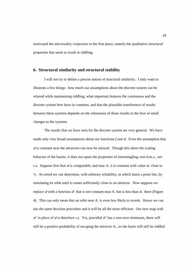
The results that we have seen for the discrete system are very general. We have

made only very broad assumptions about our functions f and α. Even the assumption that

α is constant near the attractors can now be relaxed. Though this alters the scaling

behavior of the basins, it does not upset the properties of intermingling, non-d.m.z., nor

r.a. Suppose first that α is computable, and near A+ it is constant with value α+ close to

½. As noted we can determine, with arbitrary reliability, in which basin a point lies, by

simulating its orbit until it comes sufficiently close to an attractor. Now suppose we

replace α with a function α ′ that is not constant near A+ but is less than α+ there (Figure

4). This can only mean that an orbit near A+ is even less likely to recede. Hence we can

use the same decision procedure and it will be all the more efficient. Our new map with

α ′ in place of α is therefore r.a. Yet, provided α ′ has a non-zero minimum, there will

still be a positive probability of escaping the attractor A+, so the basin will still be riddled

19

and non-d.m.z. Hence these results hold for any computable function α ′, provided only

that α ′(1) < ½ < α ′(−1), and for all y, 0 < α ′(y) < 1.

We have also assumed that, in each iteration, ϕ stretches both the left and right

portion of a horizontal all the way across the rectangle X. This too can be relaxed. As

long as ϕ effects some stretching, so that every small line segment is eventually stretched

enough to include portions of both basins, we still have intermingled basins. In fact, the

particular form of the motion in the x direction does not matter much, so long as almost

all orbits spend some time in regions that are drawn toward a given attractor [such as x <

α(y)] and some in regions that are pushed away [x > α(y)].

In these respects, Sommerer and Ott’s continuous system is very much like the

discrete system. The two attractors have stable regions (the dips in the potential) and

unstable regions (the central hump), and motion near the attractors is chaotic, spending

some time in both the stable and unstable regions. It therefore seems very plausible that,

20

Figure 4. Generalizing the discrete system. If we replace α with another computable function α ′: [–1, 1] → (0, 1) such that α ′ < α+ for y > y*, the basins are still intermingled, non-d.m.z., and recursively approximable. This holds even for α+ very close to 1/2 and y* very close to 1, so α ′ may be any computable function with α ′(1) < 1/2 and (by a parallel argument) 1/2 < α ′(–1).

like those of the discrete system, the basins of the continuous system are indeed

intermingled, non-d.m.z., and yet r.a. Sommerer and Ott may have leaned too hard on the

universal scaling conjecture, but it also seems likely that for any sufficiently regular

system with attractors, there will be some rule to the effect that most orbits near an

attractor tend toward it, so that the basins will be r.a.

Ott and his collaborators (1994; Alexander et al. 1991) discuss the important

structural features in detail. The systems in which they find riddling always have an

invariant manifold induced by a symmetry in the dynamics (like the y-symmetry in the

1996 equations). Within this there is an attractor for the subsystem within the invariant

21

manifold, and motion on this attractor is chaotic. Furthermore, the invariant manifold has

regions where nearby orbits move away from the invariant manifold and regions where

orbits are drawn closer (like the attracting dips and repelling hump in the potential V ).

Orbits within the manifold spend time in both regions. If they typically spend more time

in the attracting region, or more generally, if the net effect is attraction on the average

(negative transverse Lyapunov exponents), then the attractor for the manifold becomes an

attractor for the larger space. Yet due to the random motion of orbits through attracting

and repelling regions, there is always a non-zero chance that a particular orbit will be

repelled. Consequently, the basin are riddled. It is the recognition of these mechanisms

and structural features that leads Ott et al. to conjecture universality in the first place: the

conjecture is “[b]ased on our understanding of these results as arising from fluctuation of

the perpendicular Lyapunov exponent.”

Similar structural considerations support the conjecture that riddling is not rare.

We can illustrate this by considering how feasible it would be to manufacture a riddled or

approximately riddled12 system like Sommerer and Ott’s. This does seem achievable

12 It may be that real physical systems exhibit only approximate riddling. True riddling

requires that arbitrarily small neighborhoods in the state space contain positive-measure portions of the basin’s complement. Being non-d.m.z. similarly depends on arbitrarily small details, so if riddling is to be the basis of such undecidability, it must go “all the way down”. The plausibility of this in real-world systems is limited by two considerations.

First, Ott et al. suggest that any noise will disturb those orbits that would otherwise settle down to an attractor (1994, 392). There would still be an appearance of riddled basins, but they would not really be basins of attraction, as there would be no true attractors. Rather, almost all orbits would forever wander from one pseudo-attractor to the other. Heagy et al. observe evidence of this in their circuit.

Second, models like Sommerer and Ott’s do not accurately describe real systems on quantum scales. In particular, quantum states are governed by the linear Schrödinger equation, and riddled basins seem to require non-linearity. A classical model with riddled basins may very accurately approximate a real system, but will presumably fail where very small differences of

22

because the riddling is structurally stable: it survives small changes in the parameters of

the system. More precisely, a property is structurally stable at s0 relative to a parameter s

if there is a neighborhood U of s0 such that the property holds for all s in U. The relevant

parameters here include the amount of “friction”, the frequency and amplitude of the

periodic force, and perhaps most significantly, the coefficients determining the shape of

the surface, or the potential V. If we wished to manufacture a rocking two-welled dish

that would reproduce the erratic behavior of Sommerer and Ott’s model, the shape of the

dish would not have to be exact, for the same qualitative dynamics persist over a range of

different potentials. Ott et al. (1994) explicitly report this for potentials qualitatively

different from V, and Kan (1993) analytically proves an analogous result for certain

discrete-time systems on the thickened torus T 2 × [0, 1]. We have also seen in intuitive

terms that the riddled basins in the discrete system of 1994 persist under many broad

variations. Sommerer and Ott (1996) suggest that the same holds for their continuous

1996 system, and a handful of simulations conducted by the present author seem to

confirm this.

Intuitively, some insensitivity to the shape of the potential is to be expected, since

the riddling results from just a couple of its gross features: the two dips, which tend to

draw orbits in if friction is present, and the central hump, which tends to destabilize orbits

that run near the invariant manifold. Sommerer and Ott emphasize the importance of

initial conditions are concerned. Hence it is not clear how riddling can go “all the way down”. Quantum mechanics also puts determinism in doubt, so it is not clear what significance the notion of non-computable behavior could have. Nonetheless, riddled and non-d.m.z. sets might arise elsewhere in the quantum formalism, for example in connection with the decision problem for entanglement. (Cf. Myrvold 1997.)

23

maintaining the y-symmetry in Equations 1 and 2 in order to maintain riddling, and of

similar symmetries in other riddled systems. The symmetry guarantees the existence of

an invariant manifold, a critical part of the analysis by Sommerer and Ott and by

Alexander et al. (1992). However, even this symmetry might not be strictly necessary;

the important thing is not the symmetry per se but having a chaotic attractor in an

invariant manifold. And perhaps even an attractor that is not strictly contained in a

smooth invariant manifold could generate riddling; that remains to be seen.

Nor would the rocking of our surface have to be exactly as prescribed by

Sommerer and Ott’s equation in order to generate riddled basins. The important thing

there is that it should keep the marble moving left and right chaotically. Just about any

oscillating force with approximately the right direction, amplitude, and frequency

suffices.

All of this shows how plausible it is that the proven qualitative results for the

discrete system transfer to continuous systems with similar features. The epistemological

route this suggests is not from the discrete systems to a universal scaling law, to

validation of the simulations, and finally to riddling and intermingling, as Sommerer and

Ott indicate. Rather it is a more direct route from the riddling and intermingling of the

discrete systems to that of structurally similar continuous systems, supported

independently by the suggestive results of the simulations. Prima facie, at least, the

thorough mixing of black and white pixels in Sommerer and Ott’s graphs is epistemically

more likely if riddled basins are present than if not. Hence, by Bayes’s theorem, the

24

graphs incrementally confirm riddling. 13

7. Showing the unshowable

I have argued theses (i) and (ii) above: that Sommerer and Ott’s validation

argument fails, and that their simulations nonetheless provide compelling but fallible

evidence of riddling and non-computability, mainly by structural analogy. Thesis (iii) is

that simulations can be valuable without validation, for they can suggest and confirm

truths that we may never succeed in proving. To demand validation would be in effect to

demand proof, and thus to deprive ourselves of such insights.

I do not insist that there are absolutely unprovable truths. In one sense this is

clearly false: any self-consistent statement is provable in a theory that takes it as an

axiom. Whether there are absolutely unprovable truths in any significant sense is a

subject of ongoing discussion (e.g., Gödel [1951] 1995; Franzen 1987; Feferman 2006;

Koellner 2006). Chaitin only argues that computer experiments can illustrate facts not

provable from accepted axioms (1993). Presumably, whatever axioms of mathematics

can reasonably be considered accepted form a recursive set and imply Peano arithmetic,

13 One other method may (only they can say) have played a role in Sommerer and Ott’s

actual research: a kind of inductive bootstrapping. They assume that if a simulated orbit closely approaches an attractor, it is probably in that attractor’s basin. They use this to graph the basins. The graphs show the basins scaling in a certain way near the attractors, and this scaling, in turn, supports the original assumption that close approach indicates likely membership in the basin. Thus the simulations seem to support their own validity. To examine the formal structure and the legitimacy of such reasoning would be interesting (and Hughes notes a similar issue; 1999, 113), but tangential to our main concerns. For lack of space we can only note that, without further justification, it too remains heuristic and fallible, and in any case it is not explicitly cited in Sommerer and Ott’s validity argument.

25

so by Gödel’s theorem, they are not sufficient to prove or disprove every proposition of

arithmetic (if consistent). Hence there should be truths of mathematics that cannot be

proved from the accepted axioms. Of course, it is debatable whether the notion of

mathematical truth makes any sense independent of a set of axioms. But even within a

given theory there are at least very hard proofs. Most are too long and complex to

achieve in the near future, and unless the human race evolves to unbounded degrees of

sophistication, most will never be proved.

What Sommerer and Ott would like to prove is that the basins of their system are

riddled. It is not known whether this particular fact is provable, in any sense. In general,

though, riddling is not decidable from a formula defining a dynamical system. As a

trivial consequence of the undecidability of first-order logic, no non-trivial property of

functions (on the real numbers or any domain) is decidable from their first-order

expressions. Functions can be defined conditionally so as to depend on arbitrary

sentences. To determine the nature of all functions so defined would require deciding the

truth of all sentences. Hence, in particular, if the set of “accepted axioms” is recursive

and consistent, it cannot prove which dynamical equations result in riddled basins and

which do not. Of course, by the same token, this is not a special fact about riddling, and

it depends on permitting some rather unnatural “equations”. It would be interesting to

see which properties are decidable among a more restricted class of “ordinary” equations,

capturing those studied in dynamics.

But what is more important here is that Sommerer and Ott’s basins have not been

proven riddled, and this despite an apparent desire to do so. Sommerer and Ott do as

26

much as they can analytically, and they attempt to validate their simulations by appeal to

general principles. If they could have proved riddling, they surely would have. The main

point of their simulations is precisely to display what they cannot yet prove.

What is unprovable or unproven can nonetheless be evidenced by simulations.

Infinitary propositions, i.e., those involving unbounded quantification, are often difficult

or perhaps impossible to prove. The existence of infinitely many pairs of “twin” primes

(p, p + 2) cannot be proved or refuted by any finite number of cases, yet the many

instances found (as well as heuristic reasoning) seem to confirm the conjecture.

Similarly, the presence of riddled basins involves unbounded quantification (over time)

and is not settled by finite simulations of orbits, but as argued above, the latter do lend

confirmation.

Some think that simulations cannot display what is even practically and

temporarily unprovable, for they are merely deductions themselves. Usually, though, a

simulation is not a perfect representation of the system it simulates, even if, as in

Sommerer and Ott’s case, that system is a simple abstract model. Simulations often

involve numerical approximation methods, and their relation to their objects is complex

and “motley” (Winsberg 2001). The computation of the approximations is itself

deductive in a sense: the workings of a machine in carrying out a simulation could

arguably be interpreted as a proof of the simulation results. But what these results tell us

about the target system is not deductive unless we can add to the simulations a proof of

validity.

When the lessons of simulation are deductive, they do not serve to complement

27

deductive results. This point is independent of the question of strict unprovability. At

the very least, numerical experiments help us to see facts not yet proved. If we demand

rigorous validation before acknowledging such insights, we limit our vision to what is not

only provable, but provable within the practical bounds of time, space, and cleverness.

As long as the intermingling of Sommerer and Ott’s basins remains unproven and their

simulations not rigorously validated, those simulations provide information that is in

practice deductively unavailable. For this reason, simulations that have not been

successfully validated may be the most valuable.

Of course, this is less so if the results are false, but that worry is less urgent when

simulations serve general, theoretical purposes. If we are using simulations to design a

bridge or put someone safely on the moon, we would certainly like the strongest possible

validation of our simulations. But as claim (iv) asserts, such specific applications are not

the only functions of simulations. Sommerer and Ott’s simulations are not aimed at any

particular real-world system, but serve to inform our general expectations by revealing

qualitative features of possible systems.14 Like Lorenz’s famous weather simulations

(1963), they reveal behavior qualitatively outside of expectations. Even if we were to

discover that Sommerer and Ott’s 1996 basins are not intermingled, the cat would already

be out of the bag. The simulations would already have opened our eyes to the prima facie

possibility of such behavior in simple continuous dynamical systems, and barring reasons

14 Again, this use of simulations is not news, but it is not often acknowledged in

philosophy. Gelfert (2006) does remark on the broad, qualitative use of models, quoting a related point by Hughes (1999), but for Hughes, like Morton and Sommerer and Ott, the value of such models rests on a strict—and in Hughes’s case, precise and quantitative—universality hypothesis. The important informal use of models and simulations is not highlighted.

28

to the contrary, they would still lend plausibility to the existence of intermingled basins in

other such systems. To ignore such insights without strict validation would be unduly

skeptical. Of course, I do not claim that we should believe everything that simulations

suggest, only that they can have heuristic and evidentiary value without validation, and

for that matter, even if they are wrong!

8. Conclusions

Sommerer and Ott’s validity argument is problematic. It appeals to a conjectured

absolute, a universality, which one might hope could lead to a validity proof—but this

fails. There may be some universal scaling law, but not one specific enough to validate

the simulation. Yet there are other arguments to make. Riddling is due to certain general

structural features, and the finer details do not make much difference for the qualitative

properties of the basins. Models that have these structural features in common should

behave similarly, and simulation can serve to confirm this, rather than prove it.

Such arguments from analogy are fallible and intuitive. Perhaps they can be made

more rigorous, but science must always rest some weight on informal reasoning. Where

problems are unsolvable, intractable, or just plain hard, we do our best, and computer

simulations help a great deal. If we insist on deductive validation, then we have the

opposite problem from that of the Borges-Casares cartographers: our maps will be too

limited. They will show only the deductive train tracks, much more extensively than

before, to be sure, but revealing nothing of the wilderness between, or (if that is too

Platonistic) of the rough trails where future tracks might be laid.

29

Lastly, Sommerer and Ott’s “map” is not intended to represent any specific

territory, but a possible one, which may well resemble actual lands. It simulates an

abstract model, freely invented, far from antecedently known actual systems, and not

strongly guided by any particular force-specifying dynamical theory. If this model

mediates between theories and the world (Morton 1993; Morgan and Morrison 1999), it

does so long-distance. It has physical significance, but mainly as an example of what

kinds of behavior are possible in relatively simple systems. Like much research in non-

linear dynamics, its main function is to inform our expectations and our broader world

view.

30

REFERENCES

Alexander, J.C., J.A. Yorke, Z. You, and I. Kan. 1992. Riddled basins. International Journal of Bifurcation and Chaos 2: 795-813.

Berkovitz, J., R. Frigg, and F. Kronz. 2006. The ergodic hierarchy, decay of correlations, and Hamiltonian chaos. Studies in the History and Philosophy of Modern Physics 37: 661-991.

Borges, J.L., and A.B. Casares. [1946] 1999. On exactitude in science. Translated in Borges, Collected Fictions. Penguin.

Carroll, L. [1893] 2005. Sylvie and Bruno Concluded. http://www.hoboes.com/html/FireBlade/Carroll/Sylvie/Concluded. Retrieved 31 May, 2006.

Chaitin, G. 1993. Randomness in arithmetic and the decline and fall of reductionism in pure mathematics. EATCS Bulletin 50: 314-328.

Feferman, S. 2006. Are there absolutely unsolvable problems? Gödel’s dichotomy. Philosophia Mathematica 14: 134-152.

Franzen, T. 1987. Provability and Truth (Stockholm Studies in Philosophy 9). Stockholm: Almqvist and Wiksell International.

Gelfert, A. 2006. Simulating many-body models in physics: Rigorous results, ‘benchmarks’, and cross-model justification. PhilSci Archive: http://philsci-archive.pitt.edu/archive/00002789 .

Gödel, K. [1951] 1995. Some basic theorems on the foundations of mathematics and their implications. In K. Gödel, Collected Works, Vol. III. Unpublished Essays and Lectures. New York: Oxford University Press.

Grzegorczyk, A. 1955. Computable functionals. Fundamenta Mathematicae 42: 169-202.

Hartmann, S. 1996. The world as a process: Simulations in the natural and social sciences. In R. Hegselmann et al. (eds.), Modeling and Simulation in the Social Sciences from the Philosophy of Science Point of View. Dordrecht: Kluwer, 77-100.

Heagy, J.F., T.L. Carroll, and L.M. Pecora. 1994. Experimental and numerical evidence for riddled basins in coupled chaotic systems. Physical Review Letters 73: 3528-3531.

Hughes, R.I.G. 1999. The Ising model, computer simulation, and universal physics. In Morgan and Morrison 1999: 97-145.

Kan, I. 1994. Open sets of diffeomorphisms having two attractors, each with an everywhere

31

dense basin. Bulletin (New Series) of the American Mathematical Society 31: 68-74. Ko, K.-I. 1991. Complexity Theory of Real Functions. Boston: Birkhauser.

Koellner, P. 2006. On the question of absolute undecidability. Philosophia Mathematica 14: 153-188.

Ku, Y. H. and X. Sun. 1990. CHAOS and limit cycle in Duffing’s equation. Journal of the Franklin Institute 327: 165-195.

Lorenz, E.N. 1963. Deterministic non-periodic flow. Journal of the Atmospheric Sciences 20: 130-141.

Milnor, J. 1985. On the concept of attractor. Communications in Mathematical Physics 99: 177-195.

Morgan, M.S., and M. Morgan, eds. 1999. Models as Mediators: Perspectives on Natural and Social Science. Cambridge: Cambridge University Press.

Morton, A. 1993. Mathematical Models: Questions of Trustworthiness. British Journal for the Philosophy of Science 44: 659-674.

Myrvold, W.C. 1997. The decision problem for entanglement. In R. S. Cohen et al., eds., Potentiality, Entanglement, and Passion-at-a-Distance. Great Britain: Kluwer Academic Publishers, 177-190.

Ott, E., and J.C. Sommerer. 1994. Blowout bifurcations: the occurrence of riddled basins and on-off intermittency. Physics Letters A 188: 39-47.

Ott, E., J.C. Sommerer, J.C. Alexander, I. Kan, and J.A. Yorke. 1993. Scaling behavior of chaotic systems with riddled basins. Physical Review Letters 71: 4134–4137.

Ott, Edward, J.C. Alexander, Ittai Kan, John C. Sommerer, and James A. Yorke. 1994. The transition to chaotic attractors with riddled basins. Physica D 76: 384.

Parker, M.W. 2003. Undecidability in Rn: Riddled basins, the KAM tori, and the stability of the solar system. Philosophy of Science 70: 359-382.

–––. 2005. Undecidable long-term behavior in classical physics: Foundations, results, and interpretation. Ph.D. dissertation, University of Chicago.

–––. 2006. Three concepts of decidability for general subsets of uncountable spaces. Theoretical Computer Science 351: 2-13.

Sommerer, J.C., and E. Ott. 1996. Intermingled basins of attraction: Uncomputability in a simple physical system. Physics Letters A 214: 243-251.

Weihrauch, K. 2000. Computable Analysis: An Introduction. Berlin: Springer. Figure 5.2, p.

32

127, Chapter 5, Copyright 2000 Springer-Verlag Berlin Heidelberg, with kind permission of Springer Science and Business Media.

Winsberg, E. 2001. Simulations, models, and theories: Complex physical systems and their

representations. Philosophy of Science 68 (Proceedings): S443-S454. –––. 2003. Simulated experiments: Methodology for a virtual world. Philosophy of Science 70:

105-125.