Computing the maximum likelihood estimates: concentrated likelihood, EM ... · Computing the...
47
Computing the maximum likelihood estimates: concentrated likelihood, EM-algorithm Dmitry Pavlyuk The Mathematical Seminar, Transport and Telecommunication Institute, Riga, 13.05.2016
-
Upload
truongcong -
Category
Documents
-
view
227 -
download
0
Transcript of Computing the maximum likelihood estimates: concentrated likelihood, EM ... · Computing the...
Computing the maximum
likelihood estimates: concentrated
likelihood, EM-algorithm
Dmitry Pavlyuk
The Mathematical Seminar,
Transport and Telecommunication Institute, Riga, 13.05.2016

Presentation outline
Pavlyuk D. Computing the maximum likelihood estimates: concentrated likelihood, EM-algorithm, Riga, 13.05.2016
1. Basics of MLE
2. Pseudo-likelihood
3. Finite Mixture Models
4. The Expectation-Maximization algorithm
5. Numerical Example
2
Pavlyuk D. Computing the maximum likelihood estimates: concentrated likelihood, EM-algorithm, Riga, 13.05.2016 3
1. Basics of MLE
The estimation problem
Pavlyuk D. Computing the maximum likelihood estimates: concentrated likelihood, EM-algorithm, Riga, 13.05.2016
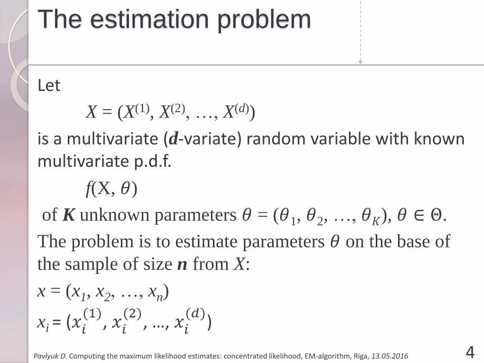
Let
X = (X(1), X(2), …, X(d))
is a multivariate (d-variate) random variable with known multivariate p.d.f.
f(X, 𝜃)
of K unknown parameters 𝜃 = (𝜃1, 𝜃2, …, 𝜃𝐾), 𝜃 ∈ Θ.
The problem is to estimate parameters 𝜃 on the base of
the sample of size n from X:
x = (x1, x2, …, xn)
xi = (𝑥𝑖(1)
, 𝑥𝑖(2)
, …, 𝑥𝑖(𝑑)
)
4

Maximum likelihood estimator
Pavlyuk D. Computing the maximum likelihood estimates: concentrated likelihood, EM-algorithm, Riga, 13.05.2016
The likelihood function 𝐿 𝜃 𝑥 represents probability of receiving the sample x given parameters 𝜃.
In case of independent observations in the sample
𝐿 𝜃 𝑥 = ෑ
𝑖=1
𝑛
𝑓 𝑥𝑖 , 𝜃
The maximum likelihood estimator is (R. Fisher, 1912+):
መ𝜃𝑚𝑙𝑒 = argmax𝜃∈Θ
𝐿 𝜃 𝑥
if a maximum exists.
5

Maximum likelihood estimator
Pavlyuk D. Computing the maximum likelihood estimates: concentrated likelihood, EM-algorithm, Riga, 13.05.2016
For computation purposes the log-likelihood function is introduced:
𝑙 𝜃 𝑥 = 𝑙𝑛𝐿 𝜃 𝑥 = 𝑙𝑛 ෑ
𝑖=1
𝑛
𝑓 𝑥𝑖 , 𝜃 =
𝑖=1
𝑛
𝑙𝑛𝑓 𝑥𝑖 , 𝜃
Good limiting statistical properties of መ𝜃𝑚𝑙𝑒:
- Consistency
- Asymptotic efficiency
- Asymptotic normality
6
Maximum likelihood estimator
Pavlyuk D. Computing the maximum likelihood estimates: concentrated likelihood, EM-algorithm, Riga, 13.05.2016
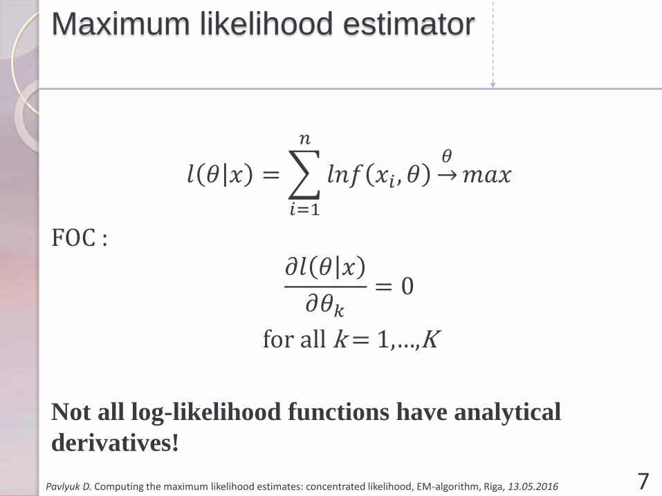
𝑙 𝜃 𝑥 =
𝑖=1
𝑛
𝑙𝑛𝑓 𝑥𝑖 , 𝜃 ՜𝜃
𝑚𝑎𝑥
FOC :𝜕𝑙 𝜃 𝑥
𝜕𝜃𝑘= 0
for all k = 1,…,K
Not all log-likelihood functions have analytical
derivatives!
7

MLE example: multivariate
normal
Pavlyuk D. Computing the maximum likelihood estimates: concentrated likelihood, EM-algorithm, Riga, 13.05.2016
For example, for the multivariate normal variable:𝑋~𝑀𝑉𝑁 𝜇, Σ𝜃𝑚𝑣𝑛 = 𝜇, Σ
𝑓𝑚𝑣𝑛 𝑥, 𝜃𝑚𝑣𝑛 = 𝜑 𝑥, 𝜇, Σ
=1
2𝜋𝑑
𝑑𝑒𝑡Σ𝑒−
12 𝑥−𝜇 𝑇Σ−1 𝑥−𝜇 =
= 2𝜋−𝑑2𝑑𝑒𝑡Σ−
12𝑒𝑥𝑝 −
1
2𝑥 − 𝜇 𝑇Σ−1 𝑥 − 𝜇
8

MLE example: multivariate
normal
Pavlyuk D. Computing the maximum likelihood estimates: concentrated likelihood, EM-algorithm, Riga, 13.05.2016
The log-likelihood function:
𝑙𝑚𝑣𝑛 𝜇, Σ 𝑥 =
𝑖=1
𝑛
𝑙𝑛𝜑 𝑥𝑖 , 𝜇, Σ =
= −𝑛𝑑
2𝑙𝑛 2𝜋 −
𝑛
2ln 𝑑𝑒𝑡Σ −
1
2
𝑖=1
𝑛
𝑥𝑖 − 𝜇 𝑇Σ−1 𝑥𝑖 − 𝜇
FOC:
𝜕𝑙𝑚𝑣𝑛 𝜇, Σ 𝑥𝜕𝜇
= 0
𝜕𝑙𝑚𝑣𝑛 𝜇, Σ 𝑥𝜕Σ
= 0
9

MLE example: multivariate
normal
Pavlyuk D. Computing the maximum likelihood estimates: concentrated likelihood, EM-algorithm, Riga, 13.05.2016
Matrix calculus (for symmetric A):
𝜕𝐵𝑇𝐴𝐵
𝜕𝐵= 2𝐵𝑇𝐴
𝜕 ln 𝑑𝑒𝑡𝐴
𝜕𝐴= 𝐴−1
10

MLE example: multivariate
normal
Pavlyuk D. Computing the maximum likelihood estimates: concentrated likelihood, EM-algorithm, Riga, 13.05.2016
𝜕𝑙𝑚𝑣𝑛 𝜇, Σ 𝑥
𝜕𝜇=
=𝜕 −
𝑛𝑑2 𝑙𝑛 2𝜋 −
𝑛2 ln 𝑑𝑒𝑡Σ −
12
σ𝑖=1𝑛 𝑥𝑖 − 𝜇 𝑇Σ−1 𝑥𝑖 − 𝜇
𝜕𝜇
=
𝑖=1
𝑛
𝑥𝑖 − 𝜇 𝑇Σ−1
Setting this to zero we obtain the pleasant result
Ƹ𝜇 Σ =1
𝑛
𝑖=1
𝑛
𝑥𝑖 = ҧ𝑥
11

MLE example: multivariate
normal
Pavlyuk D. Computing the maximum likelihood estimates: concentrated likelihood, EM-algorithm, Riga, 13.05.2016
𝜕𝑙𝑚𝑣𝑛 𝜇, Σ 𝑥
𝜕Σ=
=𝜕 −
𝑛𝑑2 𝑙𝑛 2𝜋 −
𝑛2 ln 𝑑𝑒𝑡Σ −
12
σ𝑖=1𝑛 𝑥𝑖 − 𝜇 𝑇Σ−1 𝑥𝑖 − 𝜇
𝜕Σ
=𝑛
2Σ−1 −
1
2
𝑖=1
𝑛
Σ−1 𝑥𝑖 − 𝜇 𝑥𝑖 − 𝜇 𝑇Σ−1
Setting this to zero we obtain the result
Σ =1
𝑛
𝑖=1
𝑛
𝑥𝑖 − 𝜇 𝑥𝑖 − 𝜇 𝑇
12
Pavlyuk D. Computing the maximum likelihood estimates: concentrated likelihood, EM-algorithm, Riga, 13.05.2016 13
2. Pseudo-likelihood

Pseudo-likelihood
Pavlyuk D. Computing the maximum likelihood estimates: concentrated likelihood, EM-algorithm, Riga, 13.05.2016
There are a number of suggestions for modifying the likelihood function to extract the evidence in the sample concerning a parameter of interest θA when
θ = (θA, θB).
The sample vector x is also transformed into 2 parts:
𝑥 ՜ 𝑠 = 𝑠𝐴, 𝑠𝐵
Such modifications are generally known as pseudo-likelihood functions:
• Conditional likelihood
• Marginal likelihood
• Concentrated (profile) likelihood14

Marginal likelihood
Pavlyuk D. Computing the maximum likelihood estimates: concentrated likelihood, EM-algorithm, Riga, 13.05.2016
Marginal likelihood function:
𝑓 𝑋, 𝜃 = 𝑓𝑠,𝜃 𝑠𝐴, 𝑠𝐵 , 𝜃𝐴, 𝜃𝐵 =
= 𝒇𝒎𝒂𝒓𝒈𝒊𝒏𝒂𝒍,𝑨 𝒔𝑨 𝜽𝑨 ∙ 𝑓𝑚𝑎𝑟𝑔𝑖𝑛𝑎𝑙,𝐵 𝑠𝐵 𝑠𝐴, 𝜃𝐴, 𝜃𝐵
Maximum likelihood estimates for θA are obtained by maximizing the marginal density:
𝑓𝑚𝑎𝑟𝑔𝑖𝑛𝑎𝑙,𝐴 𝑠𝐴 𝜃𝐴
Problems:
• Ignoring some of the data
• Require analytical forms of the functions 15
Conditional likelihood
Pavlyuk D. Computing the maximum likelihood estimates: concentrated likelihood, EM-algorithm, Riga, 13.05.2016
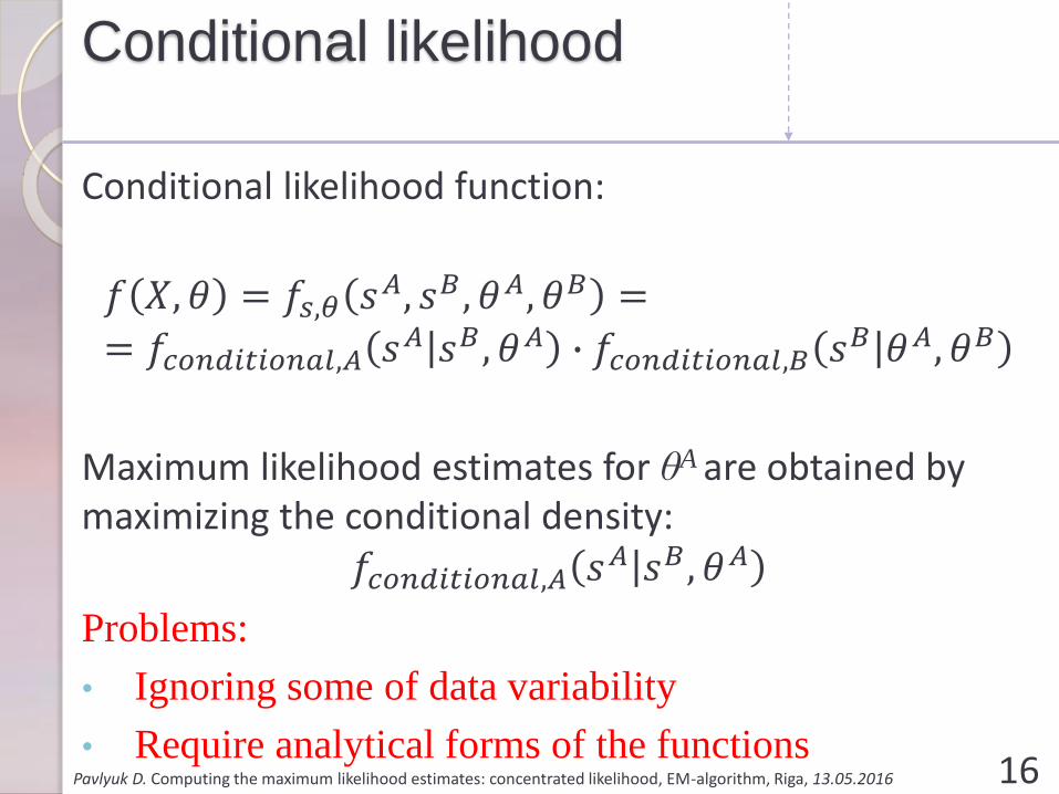
Conditional likelihood function:
𝑓 𝑋, 𝜃 = 𝑓𝑠,𝜃 𝑠𝐴, 𝑠𝐵 , 𝜃𝐴, 𝜃𝐵 =
= 𝑓𝑐𝑜𝑛𝑑𝑖𝑡𝑖𝑜𝑛𝑎𝑙,𝐴 𝑠𝐴 𝑠𝐵 , 𝜃𝐴 ∙ 𝑓𝑐𝑜𝑛𝑑𝑖𝑡𝑖𝑜𝑛𝑎𝑙,𝐵 𝑠𝐵 𝜃𝐴, 𝜃𝐵
Maximum likelihood estimates for θA are obtained by maximizing the conditional density:
𝑓𝑐𝑜𝑛𝑑𝑖𝑡𝑖𝑜𝑛𝑎𝑙,𝐴 𝑠𝐴 𝑠𝐵 , 𝜃𝐴
Problems:
• Ignoring some of data variability
• Require analytical forms of the functions16
Concentrated likelihood
Pavlyuk D. Computing the maximum likelihood estimates: concentrated likelihood, EM-algorithm, Riga, 13.05.2016
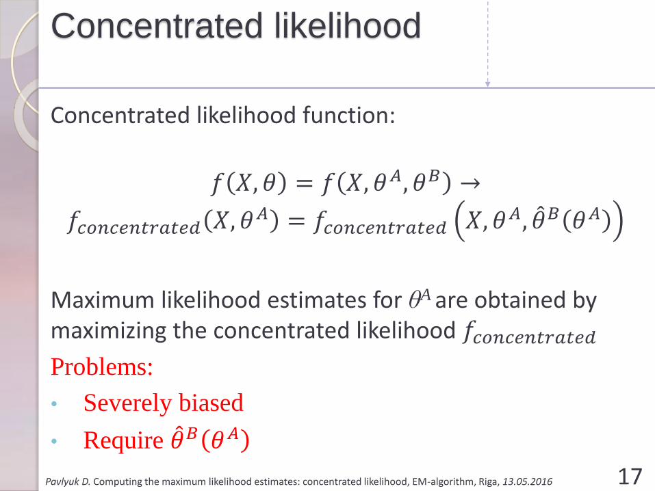
Concentrated likelihood function:
𝑓 𝑋, 𝜃 = 𝑓 𝑋, 𝜃𝐴, 𝜃𝐵 ՜
𝑓𝑐𝑜𝑛𝑐𝑒𝑛𝑡𝑟𝑎𝑡𝑒𝑑 𝑋, 𝜃𝐴 = 𝑓𝑐𝑜𝑛𝑐𝑒𝑛𝑡𝑟𝑎𝑡𝑒𝑑 𝑋, 𝜃𝐴, መ𝜃𝐵 𝜃𝐴
Maximum likelihood estimates for θA are obtained by maximizing the concentrated likelihood 𝑓𝑐𝑜𝑛𝑐𝑒𝑛𝑡𝑟𝑎𝑡𝑒𝑑
Problems:
• Severely biased
• Require መ𝜃𝐵 𝜃𝐴
17
Concentrated likelihood
Pavlyuk D. Computing the maximum likelihood estimates: concentrated likelihood, EM-algorithm, Riga, 13.05.2016
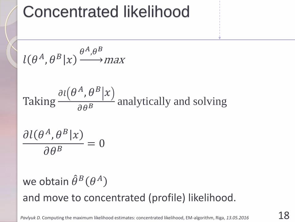
𝑙 𝜃𝐴, 𝜃𝐵 𝑥𝜃𝐴,𝜃𝐵
max
Taking 𝜕𝑙 𝜃𝐴, 𝜃𝐵 𝑥
𝜕𝜃𝐵 analytically and solving
𝜕𝑙 𝜃𝐴, 𝜃𝐵 𝑥
𝜕𝜃𝐵= 0
we obtain መ𝜃𝐵 𝜃𝐴
and move to concentrated (profile) likelihood.
18
Concentrated likelihood
Pavlyuk D. Computing the maximum likelihood estimates: concentrated likelihood, EM-algorithm, Riga, 13.05.2016
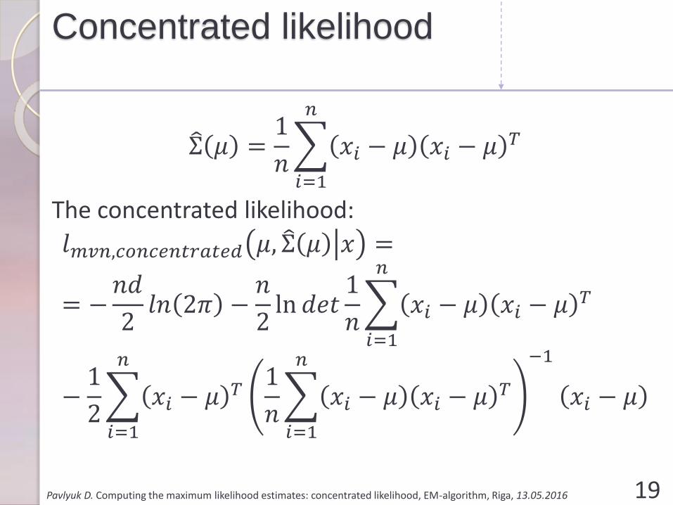
Σ 𝜇 =1
𝑛
𝑖=1
𝑛
𝑥𝑖 − 𝜇 𝑥𝑖 − 𝜇 𝑇
The concentrated likelihood:
𝑙𝑚𝑣𝑛,𝑐𝑜𝑛𝑐𝑒𝑛𝑡𝑟𝑎𝑡𝑒𝑑 𝜇, Σ 𝜇 𝑥 =
= −𝑛𝑑
2𝑙𝑛 2𝜋 −
𝑛
2ln 𝑑𝑒𝑡
1
𝑛
𝑖=1
𝑛
𝑥𝑖 − 𝜇 𝑥𝑖 − 𝜇 𝑇
−1
2
𝑖=1
𝑛
𝑥𝑖 − 𝜇 𝑇1
𝑛
𝑖=1
𝑛
𝑥𝑖 − 𝜇 𝑥𝑖 − 𝜇 𝑇
−1
𝑥𝑖 − 𝜇
19

Concentrated likelihood
Pavlyuk D. Computing the maximum likelihood estimates: concentrated likelihood, EM-algorithm, Riga, 13.05.2016
𝑙𝑚𝑣𝑛,𝑐𝑜𝑛𝑐𝑒𝑛𝑡𝑟𝑎𝑡𝑒𝑑 𝜇, Σ 𝜇 𝑥 =
= −𝑛
2𝑑 ∙ 𝑙𝑛 2𝜋 + ln 𝑑𝑒𝑡
𝑖=1
𝑛
𝑥𝑖 − 𝜇 𝑥𝑖 − 𝜇 𝑇 + 𝑑
ෝ𝜇 = argmin𝜇
ln 𝑑𝑒𝑡
𝑖=1
𝑛
𝑥𝑖 − 𝜇 𝑥𝑖 − 𝜇 𝑇
This result is quite famous in econometrics!
20

Pavlyuk D. Computing the maximum likelihood estimates: concentrated likelihood, EM-algorithm, Riga, 13.05.2016 21
3. Finite Mixture Models
Gaussian mixture model
Pavlyuk D. Computing the maximum likelihood estimates: concentrated likelihood, EM-algorithm, Riga, 13.05.2016
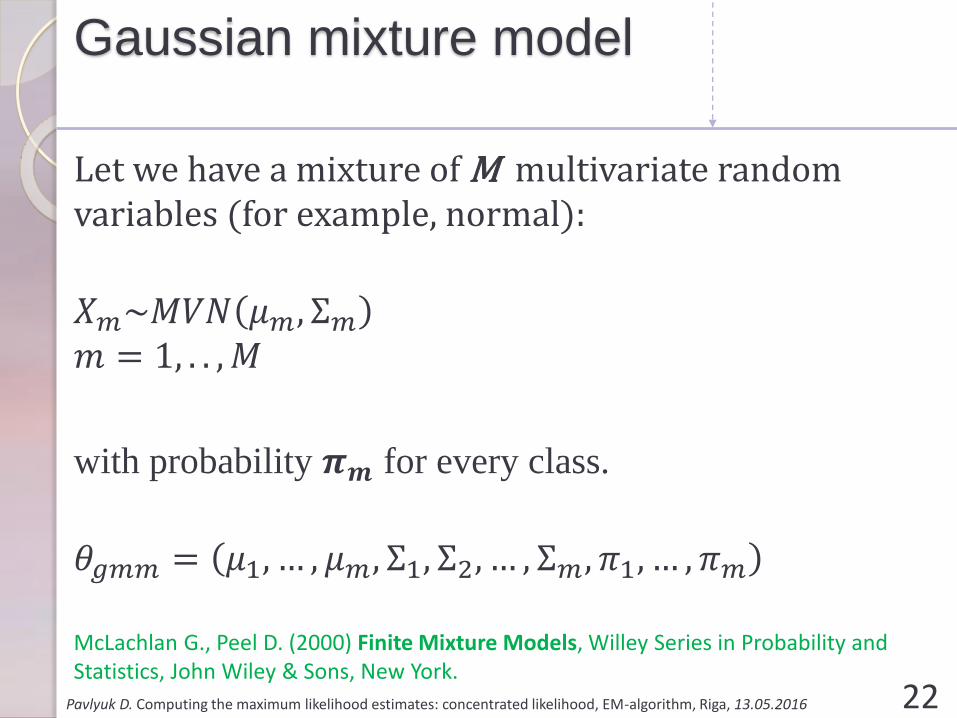
Let we have a mixture of M multivariate random variables (for example, normal):
𝑋𝑚~𝑀𝑉𝑁 𝜇𝑚, Σ𝑚
𝑚 = 1, . . , 𝑀
with probability 𝝅𝒎 for every class.
𝜃𝑔𝑚𝑚 = 𝜇1, … , 𝜇𝑚, Σ1, Σ2, … , Σ𝑚, 𝜋1, … , 𝜋𝑚
McLachlan G., Peel D. (2000) Finite Mixture Models, Willey Series in Probability and Statistics, John Wiley & Sons, New York.
22
Gaussian mixture model
Pavlyuk D. Computing the maximum likelihood estimates: concentrated likelihood, EM-algorithm, Riga, 13.05.2016
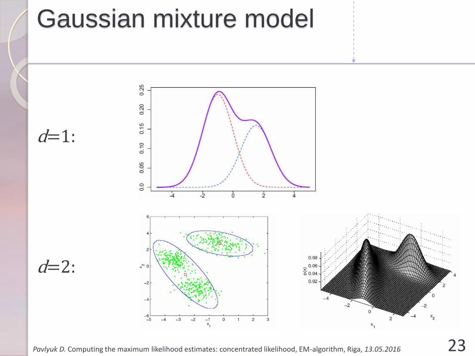
d=1:
d=2:
23
Gaussian mixture model
Pavlyuk D. Computing the maximum likelihood estimates: concentrated likelihood, EM-algorithm, Riga, 13.05.2016
• Medical applicationsSchlattmann P. (2009) Medical Applications of Finite Mixture Models, Statistics for Biology and Health, Springer
• Financial applicationsBrigo, D.; Mercurio, F. (2002). Lognormal-mixture dynamics and calibration to market volatility smiles
Alexander, C. (2004). "Normal mixture diffusion with uncertain volatility: Modelling short- and long-term smile effects"
• Image, speech, text recognitionStylianou, Y. etc. (2005). GMM-Based Multimodal Biometric Verification
Reynolds, D., Rose, R. (1995). Robust text-independent speaker identification using Gaussian mixture speaker models
Permuter, H.; Francos, J.; Jermyn, I.H. (2003). Gaussian mixture models of texture and colour for image database retrieval.
24

Gaussian mixture model
Pavlyuk D. Computing the maximum likelihood estimates: concentrated likelihood, EM-algorithm, Riga, 13.05.2016
Following the law of complete probability, the likelihood
function is
𝐿𝑔𝑚𝑚 𝜃𝑔𝑚𝑚 𝑥 = ෑ
𝑖=1
𝑛
𝑚=1
𝑀
𝜋𝑚𝜑 𝑥𝑖 , 𝜇𝑚, Σ𝑚
𝑙𝑔𝑚𝑚 𝜃𝑔𝑚𝑚 𝑥 = 𝑙𝑛𝐿𝑔𝑚𝑚 𝜃𝑔𝑚𝑚 𝑥 = 𝑙𝑛 ෑ
𝑖=1
𝑛
𝑚=1
𝑀
𝜋𝑚𝜑 𝑥𝑖 , 𝜇𝑚, Σ𝑚
=
𝑖=1
𝑛
𝑙𝑛 𝜋1𝜑 𝑥𝑖 , 𝜇1, Σ1 + ⋯ + 𝜋𝑚𝜑 𝑥𝑖 , 𝜇𝑚, Σ𝑚
The logarithm of sum prevents analytical derivatives!
25
Pavlyuk D. Computing the maximum likelihood estimates: concentrated likelihood, EM-algorithm, Riga, 13.05.2016 26
4. The Expectation-Maximization
algorithm

EM-algorithm
Pavlyuk D. Computing the maximum likelihood estimates: concentrated likelihood, EM-algorithm, Riga, 13.05.2016
The expectation-maximization (EM) algorithm is a general method for finding maximum likelihood estimates when there are missing values or latent variables.
In the mixture model context, the missing data is represented by a set of observations of a discrete random variable Z that indicates which mixture component generated the observation i.
𝑧𝑖𝑚 = ቊ1, 𝑖𝑓 𝑜𝑏𝑠𝑒𝑟𝑣𝑎𝑡𝑖𝑜𝑛 𝑖 𝑏𝑒𝑙𝑜𝑛𝑔𝑠 𝑡𝑜 𝑐𝑙𝑎𝑠𝑠 𝑚,
0, 𝑜𝑡ℎ𝑒𝑟𝑤𝑖𝑠𝑒
27

EM-algorithm: GMM
Pavlyuk D. Computing the maximum likelihood estimates: concentrated likelihood, EM-algorithm, Riga, 13.05.2016
𝑧𝑖𝑚 = ቊ1, 𝑖𝑓 𝑜𝑏𝑠𝑒𝑟𝑣𝑎𝑡𝑖𝑜𝑛 𝑖 𝑏𝑒𝑙𝑜𝑛𝑔𝑠 𝑡𝑜 𝑐𝑙𝑎𝑠𝑠 𝑚,
0, 𝑜𝑡ℎ𝑒𝑟𝑤𝑖𝑠𝑒
If Z = {zim} is given,
𝑙𝑔𝑚𝑚 𝜃𝑔𝑚𝑚 𝑥 =
𝑖=1
𝑛
𝑙𝑛 𝜋1𝜑 𝑥𝑖 , 𝜇1, Σ1 + ⋯ + 𝜋𝑚𝜑 𝑥𝑖 , 𝜇𝑚, Σ𝑚
transformed to
𝑙𝑔𝑚𝑚,𝑐𝑜𝑚𝑝𝑙𝑒𝑡𝑒 𝜃𝑔𝑚𝑚 𝑥, 𝑍 =
𝑖=1
𝑛
𝑚=1
𝑀
𝑧𝑖,𝑚𝑙𝑛 𝜋𝑚𝜑 𝑥𝑖 , 𝜇𝑚, Σ𝑚 =
=
𝑖=1
𝑛
𝑚=1
𝑀
𝑧𝑖,𝑚 𝑙𝑛𝜋𝑚 + 𝑙𝑛𝜑 𝑥𝑖 , 𝜇𝑚, Σ𝑚
28
EM-algorithm
Pavlyuk D. Computing the maximum likelihood estimates: concentrated likelihood, EM-algorithm, Riga, 13.05.2016
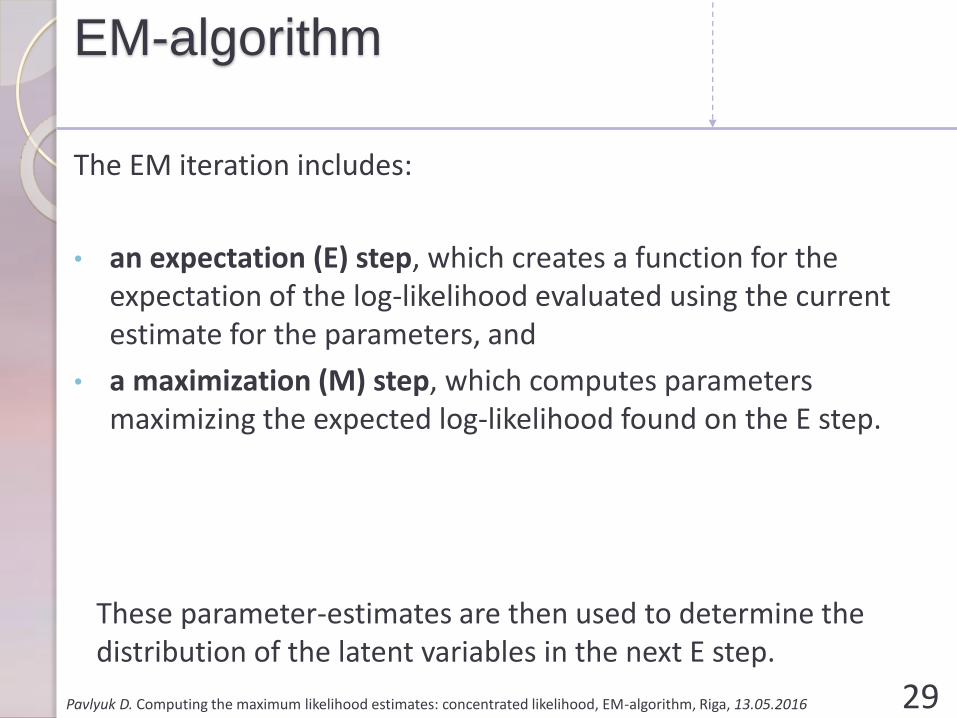
The EM iteration includes:
• an expectation (E) step, which creates a function for the expectation of the log-likelihood evaluated using the current estimate for the parameters, and
• a maximization (M) step, which computes parameters maximizing the expected log-likelihood found on the E step.
29
These parameter-estimates are then used to determine the distribution of the latent variables in the next E step.

EM-algorithm: GMM
Pavlyuk D. Computing the maximum likelihood estimates: concentrated likelihood, EM-algorithm, Riga, 13.05.2016
Assume 𝜃𝑔𝑚𝑚(0)
and move to maximization of the
expectation of the log-likelihood function:
𝐸𝑍 𝑙𝑔𝑚𝑚,𝑐𝑜𝑚𝑝𝑙𝑒𝑡𝑒 𝜃𝑔𝑚𝑚(0)
𝑥, 𝑍
=
𝑖=1
𝑛
𝑚=1
𝑀
𝐸𝑍 𝑧𝑖,𝑚 𝜃𝑔𝑚𝑚(0)
𝑙𝑛𝜋𝑚 + 𝑙𝑛𝜑 𝑥𝑖 , 𝜇𝑚, Σ𝑚
30
EM-algorithm: E-step
Pavlyuk D. Computing the maximum likelihood estimates: concentrated likelihood, EM-algorithm, Riga, 13.05.2016
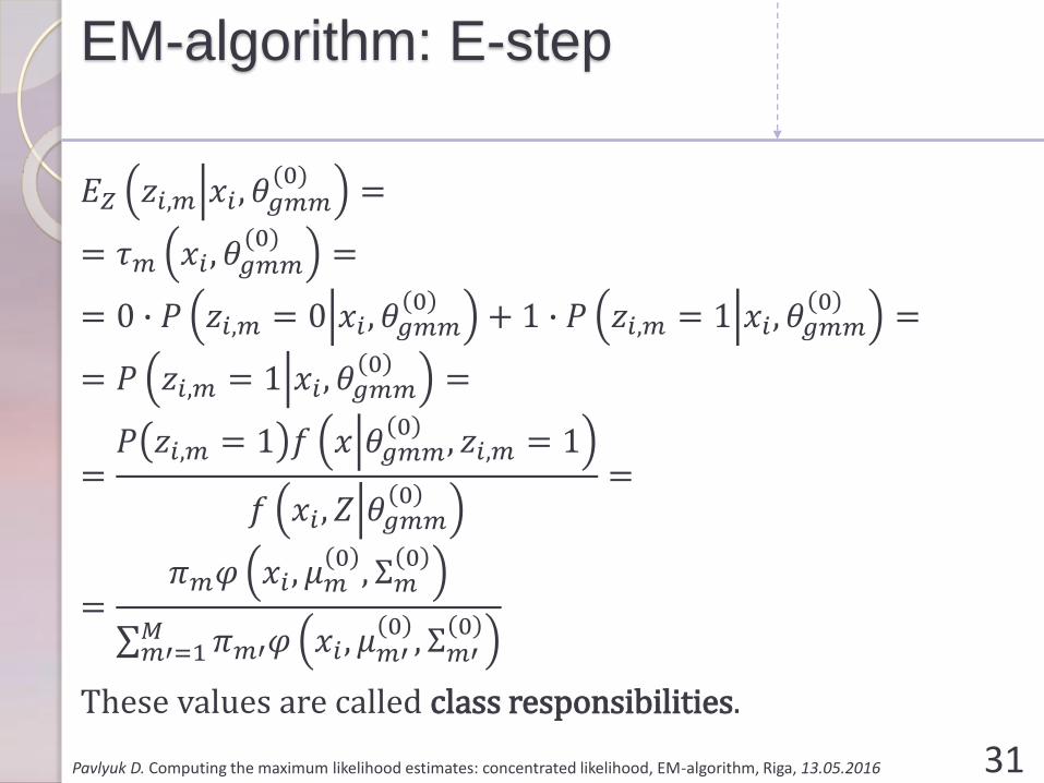
𝐸𝑍 𝑧𝑖,𝑚 𝑥𝑖 , 𝜃𝑔𝑚𝑚(0)
=
= 𝜏𝑚 𝑥𝑖 , 𝜃𝑔𝑚𝑚(0)
=
= 0 ∙ 𝑃 𝑧𝑖,𝑚 = 0 𝑥𝑖 , 𝜃𝑔𝑚𝑚0
+ 1 ∙ 𝑃 𝑧𝑖,𝑚 = 1 𝑥𝑖 , 𝜃𝑔𝑚𝑚0
=
= 𝑃 𝑧𝑖,𝑚 = 1 𝑥𝑖 , 𝜃𝑔𝑚𝑚0
=
=𝑃 𝑧𝑖,𝑚 = 1 𝑓 𝑥 𝜃𝑔𝑚𝑚
0, 𝑧𝑖,𝑚 = 1
𝑓 𝑥𝑖 , 𝑍 𝜃𝑔𝑚𝑚0
=
=𝜋𝑚𝜑 𝑥𝑖 , 𝜇𝑚
0, Σ𝑚
0
σ𝑚′=1𝑀 𝜋𝑚′𝜑 𝑥𝑖 , 𝜇𝑚′
0, Σ𝑚′
0
These values are called class responsibilities.
31

EM-algorithm: M-step
Pavlyuk D. Computing the maximum likelihood estimates: concentrated likelihood, EM-algorithm, Riga, 13.05.2016
𝐸𝑍 𝑙𝑔𝑚𝑚,𝑐𝑜𝑚𝑝𝑙𝑒𝑡𝑒 𝜃𝑔𝑚𝑚(0)
𝑥, 𝑍
=
𝑖=1
𝑛
𝑚=1
𝑀
𝜏𝑚 𝑥𝑖 , 𝜃𝑔𝑚𝑚(0)
𝑙𝑛𝜋𝑚 + 𝑙𝑛𝜑 𝑥𝑖 , 𝜇𝑚, Σ𝑚
FOC:
𝜕𝐸 𝑙𝑔𝑚𝑚,𝑐𝑜𝑚𝑝𝑙𝑒𝑡𝑒 𝜃𝑔𝑚𝑚(0)
𝑥, 𝑍
𝜕𝜇𝑚= 0,
𝜕𝐸 𝑙𝑔𝑚𝑚,𝑐𝑜𝑚𝑝𝑙𝑒𝑡𝑒 𝜃𝑔𝑚𝑚(0)
𝑥, 𝑍
𝜕Σ𝑚= 0,
𝜕𝐸 𝑙𝑔𝑚𝑚,𝑐𝑜𝑚𝑝𝑙𝑒𝑡𝑒 𝜃𝑔𝑚𝑚(0)
𝑥, 𝑍
𝜕𝜋𝑚= 0
32

EM-algorithm: M-step
Pavlyuk D. Computing the maximum likelihood estimates: concentrated likelihood, EM-algorithm, Riga, 13.05.2016
𝜕𝐸𝑍 𝑙𝑐𝑜𝑚𝑝𝑙𝑒𝑡𝑒 𝜃𝑔𝑚𝑚(0)
𝑥, 𝑍
𝜕𝜇𝑚=
𝑖=1
𝑛
𝜏𝑚 𝑥𝑖 , 𝜃𝑔𝑚𝑚(0) 𝜕𝜑 𝑥𝑖 , 𝜇𝑚, Σ𝑚
𝜕𝜇𝑚
=
𝑖=1
𝑛
𝜏𝑚 𝑥𝑖 , 𝜃𝑔𝑚𝑚(0)
𝑥𝑖 − 𝜇𝑚𝑇Σ−1 = 0
Ƹ𝜇𝑔𝑚𝑚,𝑚(1)
=σ𝑖=1
𝑛 𝜏𝑚 𝑥𝑖 , 𝜃𝑔𝑚𝑚(0)
𝑥𝑖
σ𝑖=1𝑛 𝜏𝑚 𝑥𝑖 , 𝜃𝑔𝑚𝑚
(0)
33

EM-algorithm: M-step
Pavlyuk D. Computing the maximum likelihood estimates: concentrated likelihood, EM-algorithm, Riga, 13.05.2016
𝜕𝐸𝑍 𝑙𝑐𝑜𝑚𝑝𝑙𝑒𝑡𝑒 𝜃𝑔𝑚𝑚(0)
𝑥, 𝑍
𝜕Σ𝑚=
𝑖=1
𝑛
𝜏𝑚 𝑥𝑖 , 𝜃𝑔𝑚𝑚(0) 𝜕𝜑 𝑥𝑖 , 𝜇𝑚, Σ𝑚
𝜕Σ𝑚=
=
𝑖=1
𝑛
𝜏𝑚 𝑥𝑖 , 𝜃𝑔𝑚𝑚(0) 𝑛
2Σ𝑚
−1 −1
2
𝑖=1
𝑛
Σ𝑚−1 𝑥𝑖 − 𝜇𝑚 𝑥𝑖 − 𝜇𝑚
𝑇Σ𝑚−1
Σ𝑔𝑚𝑚,𝑚(1)
=σ𝑖=1
𝑛 𝜏𝑚 𝑥𝑖 , 𝜃𝑔𝑚𝑚(0)
𝑥𝑖 − Ƹ𝜇𝑔𝑚𝑚,𝑚(0)
𝑥𝑖 − ො𝜇𝑔𝑚𝑚,𝑚(0) 𝑇
σ𝑖=1𝑛 𝜏𝑚 𝑥𝑖 , 𝜃𝑔𝑚𝑚
(0)
34
EM-algorithm: M-step
Pavlyuk D. Computing the maximum likelihood estimates: concentrated likelihood, EM-algorithm, Riga, 13.05.2016
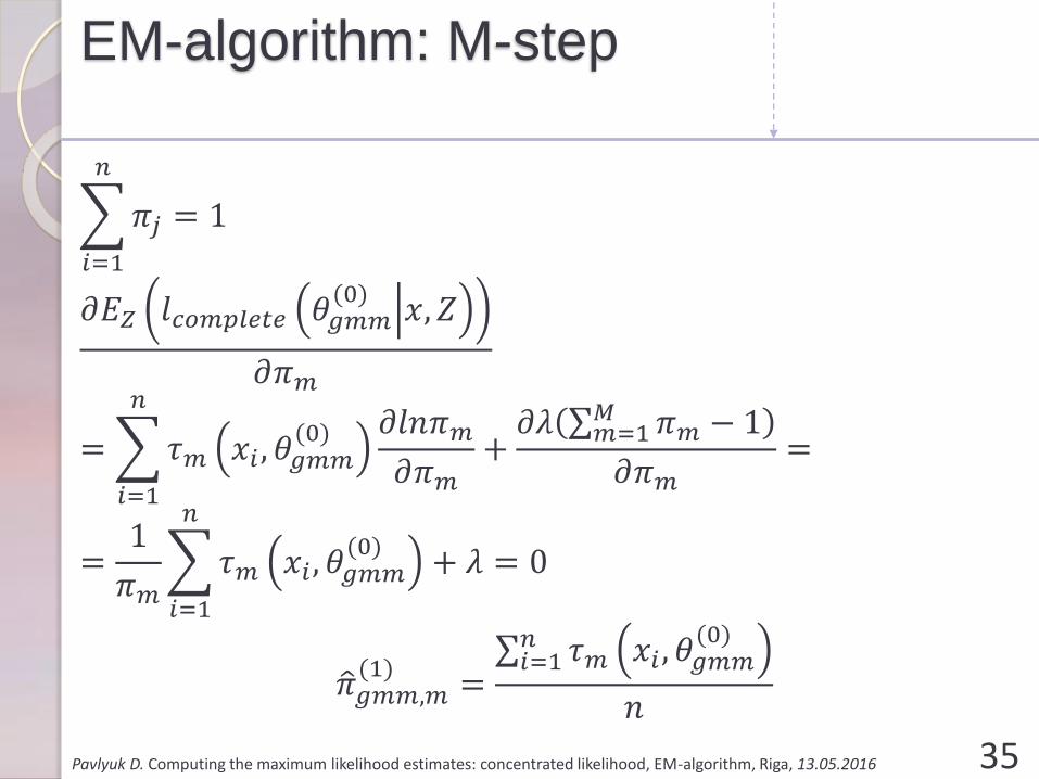
𝑖=1
𝑛
𝜋𝑗 = 1
𝜕𝐸𝑍 𝑙𝑐𝑜𝑚𝑝𝑙𝑒𝑡𝑒 𝜃𝑔𝑚𝑚(0)
𝑥, 𝑍
𝜕𝜋𝑚
=
𝑖=1
𝑛
𝜏𝑚 𝑥𝑖 , 𝜃𝑔𝑚𝑚(0) 𝜕𝑙𝑛𝜋𝑚
𝜕𝜋𝑚+
𝜕𝜆 σ𝑚=1𝑀 𝜋𝑚 − 1
𝜕𝜋𝑚=
=1
𝜋𝑚
𝑖=1
𝑛
𝜏𝑚 𝑥𝑖 , 𝜃𝑔𝑚𝑚(0)
+ 𝜆 = 0
ො𝜋𝑔𝑚𝑚,𝑚(1)
=σ𝑖=1
𝑛 𝜏𝑚 𝑥𝑖 , 𝜃𝑔𝑚𝑚(0)
𝑛
35
EM-algorithm
Pavlyuk D. Computing the maximum likelihood estimates: concentrated likelihood, EM-algorithm, Riga, 13.05.2016
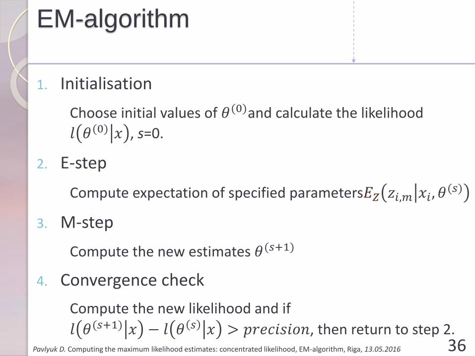
1. Initialisation
Choose initial values of 𝜃(0)and calculate the likelihood
𝑙 𝜃(0) 𝑥 , s=0.
2. E-step
Compute expectation of specified parameters𝐸𝑍 𝑧𝑖,𝑚 𝑥𝑖 , 𝜃(𝑠)
3. M-step
Compute the new estimates 𝜃(𝑠+1)
4. Convergence check
Compute the new likelihood and if
𝑙 𝜃(𝑠+1) 𝑥 − 𝑙 𝜃 𝑠 𝑥 > 𝑝𝑟𝑒𝑐𝑖𝑠𝑖𝑜𝑛, then return to step 2.36

EM-algorithm
Pavlyuk D. Computing the maximum likelihood estimates: concentrated likelihood, EM-algorithm, Riga, 13.05.2016
Dempster, Laird, and Rubin (1977) show that the
likelihood function 𝑙 𝜃(𝑠) 𝑥 is not decreased after an
EM iteration; that is
𝑙 𝜃(𝑠+1) 𝑥 ≥ 𝑙 𝜃(𝑠) 𝑥
for s = 0,1,2, ....
See the proof in:McLachlan G.J., Krishnan T. (1997) The EM Algorithm and Extensions, Wiley. — 304 p.
37

Pavlyuk D. Computing the maximum likelihood estimates: concentrated likelihood, EM-algorithm, Riga, 13.05.2016 38
5. Numerical Example
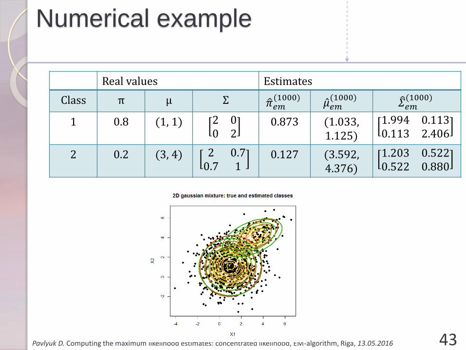
Numerical example
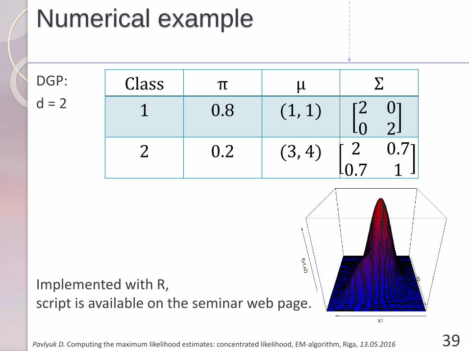
Pavlyuk D. Computing the maximum likelihood estimates: concentrated likelihood, EM-algorithm, Riga, 13.05.2016
DGP:
d = 2
Implemented with R,script is available on the seminar web page.
39
Class π μ Σ
1 0.8 (1, 1) 2 00 2
2 0.2 (3, 4) 2 0.70.7 1
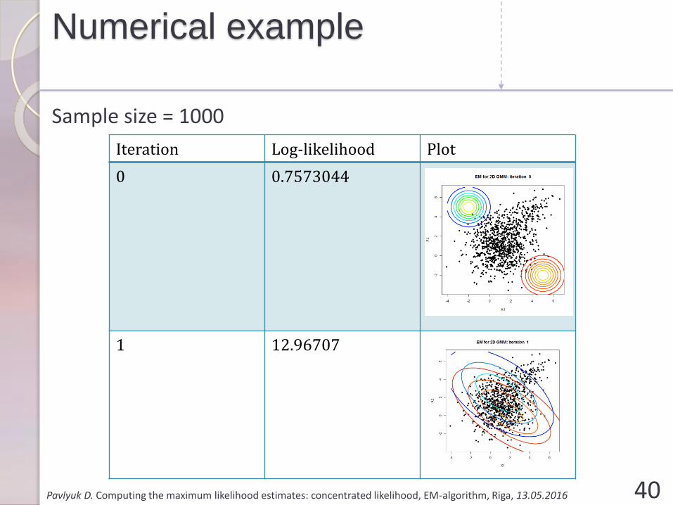
Numerical example
Pavlyuk D. Computing the maximum likelihood estimates: concentrated likelihood, EM-algorithm, Riga, 13.05.2016
Sample size = 1000
40
Iteration Log-likelihood Plot
0 0.7573044
1 12.96707
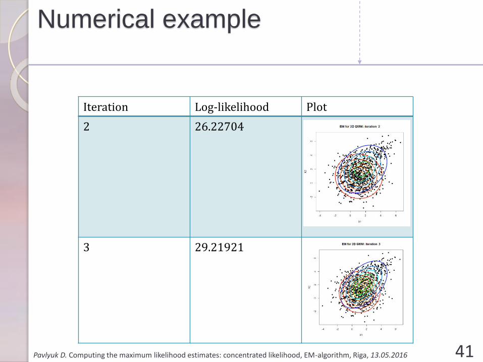
Numerical example
Pavlyuk D. Computing the maximum likelihood estimates: concentrated likelihood, EM-algorithm, Riga, 13.05.2016 41
Iteration Log-likelihood Plot
2 26.22704
3 29.21921
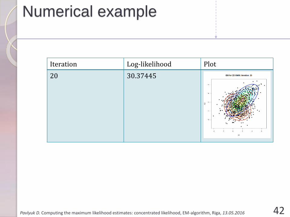
Numerical example
Pavlyuk D. Computing the maximum likelihood estimates: concentrated likelihood, EM-algorithm, Riga, 13.05.2016 42
Iteration Log-likelihood Plot
20 30.37445
Numerical example
Pavlyuk D. Computing the maximum likelihood estimates: concentrated likelihood, EM-algorithm, Riga, 13.05.2016 43
Real values Estimates
Class π μ Σ ො𝜋𝑒𝑚(1000)
Ƹ𝜇𝑒𝑚(1000) 𝛴𝑒𝑚
(1000)
1 0.8 (1, 1) 2 00 2
0.873 (1.033, 1.125)
1.994 0.1130.113 2.406
2 0.2 (3, 4) 2 0.70.7 1
0.127 (3.592, 4.376)
1.203 0.5220.522 0.880

Problems with EM
Pavlyuk D. Computing the maximum likelihood estimates: concentrated likelihood, EM-algorithm, Riga, 13.05.2016
• Local maxima
• partially solved with careful (repetitive) initial values selection
• Slow convergence (in some cases)
• Meta-algorithm
• should be adapted for every specific problem
• Singularities and over-fitting
44

After EM
Pavlyuk D. Computing the maximum likelihood estimates: concentrated likelihood, EM-algorithm, Riga, 13.05.2016
Next step:
Variational Bayes
• treat all parameters θ as missing variables
• iterate over components of missing variables (including θ) and recalculate its expectation
45
Recommended literature
Pavlyuk D. Computing the maximum likelihood estimates: concentrated likelihood, EM-algorithm, Riga, 13.05.2016
• McLachlan G., Krishnan T. (2008) The EM Algorithm and Extensions, Wiley Series in Probability and Statistics, 2nd Edition, - 400 p.
• McLachlan G., Peel D. (2000) Finite Mixture Models, Willey Series in Probability and Statistics, John Wiley & Sons, New York
• Gelman A., Carlin J., Stern H., Dunson D., Vehtari A., Rubin D. Bayesian Data Analysis, Third Edition (Chapman & Hall/CRC Texts in Statistical Science) http://www.stat.columbia.edu/~gelman/book/
46

Thank you for your attention!
Questions are very appreciated
Contacts:
email: [email protected]
phone: +37129958338